Freiburg–THEP 97–04

UM–TH–97–06

February 1997

Massive two–loop integrals in renormalizable theories
Adrian Ghinculov^a and York–Peng Yao^b

^aAlbert–Ludwigs–Universität Freiburg, Fakultät für Physik,
Hermann–Herder Str.3, D-79104 Freiburg, Germany
^bRandall Laboratory of Physics, University of Michigan,
Ann Arbor, Michigan 48109–1120, USA

We propose a framework for calculating two–loop Feynman diagrams which appear within a renormalizable theory in the general mass case and at finite external momenta. Our approach is a combination of analytical results and of high accuracy numerical integration, similar to a method proposed previously [10] for treating diagrams without numerators. We reduce all possible tensor structures to a small set of scalar integrals, for which we provide integral representations in terms of four basic functions. The algebraic part is suitable for implementing in a computer program for the automatic generation and evaluation of Feynman graphs. The numerical part is essentially the same as in the case of Feynman diagrams without numerators.

Abstract

We propose a framework for calculating two–loop Feynman diagrams which appear within a renormalizable theory in the general mass case and at finite external momenta. Our approach is a combination of analytical results and of high accuracy numerical integration, similar to a method proposed previously [10] for treating diagrams without numerators. We reduce all possible tensor structures to a small set of scalar integrals, for which we provide integral representations in terms of four basic functions. The algebraic part is suitable for implementing in a computer program for the automatic generation and evaluation of Feynman graphs. The numerical part is essentially the same as in the case of Feynman diagrams without numerators.

1 Introduction

The importance of developing techniques to calculate radiative corrections can hardly be overemphasized. The measurements at existing high energy colliders, like LEP and the SLC, are clearly sensitive to one–loop electroweak effects. As their precision increases, analyses at two–loop level may become necessary [1].

The problem of calculating one–loop Feynman diagrams was in principle solved completely long time ago by ’t Hooft and Veltman [2], and by Passarino and Veltman [3]. For a review, see for instance ref. [4], and refs. [5, 6] for some applications. As it is well–known, all one–loop diagrams are expressible in terms of Spence functions. In the general mass case, however, the numerical evaluation of the resulting expressions may be tricky [7]. This is because one needs to take care that the functions involved remain on the correct Riemann sheet, and because one has to control potentially large numerical cancellations.

No similar general solution was available so far at two–loop level in the general massive case, although a lot of effort was devoted to solving two–loop massive integrals at finite external momenta. There are two issues involved, given a general diagram with particles with spins: First, the numerator of the amplitude usually has non-trivial tensorial structures. It is convenient for us to decompose the amplitude into various tensorial constructs made of external momenta and metric tensors, multiplied by scalar functions, which in turn must be related back to the original Feynman integral by certain projections. Second, one should advance an algorithm by which one can evaluate these generalized scalar integrals, which have non-trivial numerators, in a systematic and, better yet, universal way.

Regarding the evaluation of two–loop scalar integrals, a lot of work was done in this direction lately, and it has become clear that in general the integrals involved at two–loop level are not expressible analytically in terms of well–known and easy to evaluate functions like polylogarithms, as is the case with one–loop diagrams. Partly numerical approaches seem unavoidable in the general mass case. Only in some rare situations is an analytical solution in terms of special functions known. Such an example is ref. [9], where a certain two–loop self–energy diagram was related to the Lauricella functions. A large number of approaches were proposed which work for specific topologies or mass combinations - see, for instance, refs. [9]—[22] and references therein. In most cases, these works deal with Feynman integrals with simplified couplings and numerators. Some of these approaches can yield precise numerical results for the diagrams to which they apply; by combining several such methods, one was able to apply them to actual physical processes. While they do hold promise to be extendable to cover more complicated scalar integrals which may appear in processes involving particles with spin, derivative couplings, and more external momenta, it is fair to say that this program has not been completed so far. Moreover, for calculating a physical process, such approaches would involve separate methods to treat individual graphs. This implies a considerable amount of work which grows very fast with the complexity of the process considered.

Fewer results exist concerning the reduction of two–loop Feynman graphs to scalar integrals. In ref. [23] it was shown that the two–loop self–energy diagrams can be reduced to scalar integrals without numerators. This result applies only to two–point functions. It was used in conjunction with numerical integration in ref. [24] for calculating certain two–loop contributions to the $\rho$ parameter. The approach of ref. [23] only refers to propagator diagrams. Ref. [25], which also deals with propagator diagrams, might be extendable to some more complicated diagrams, like certain 3-point functions in simplified kinematic cases, and the recurrence relations of ref. [25] perhaps can be solved numerically in more complicated cases, as suggested in the Conclusions of ref. [25].

Compared to the approaches briefly discussed above, in this paper we present a general universal framework which applies to any n-particle 2-loop diagram with arbitrary renormalizable dynamics and any combination of masses and external momenta. Strictly speaking, our formulae can be used directly for calculating one given diagram only if that diagram is free of mass singularities. However, in actual calculations this can be often circumvented by isolating the singularity analytically at the level of the integrand, by considering infrared finite sums of diagrams, or by introducing a mass regulator, as was possible for instance in ref. [12]. In our approach, all diagrams are treated using the same algorithm, and for this reason the whole calculation, including the generation of the relevant diagrams, can be authomatized. This was done in ref. [10] in a simplified case of $H\rightarrow WW$ decay, which involves no tensor structures in the numerator, and is a subset of what we shall discuss in this paper. This can be compared with ref. [15], whose authors used separate methods for individual diagrams to perform the same calculation, and which is so far the state–of–the–art of physical calculations by using these methods.

Within the framework which we propose, we shall show that in any renormalizable theory all two–loop diagrams can be expressed in terms of a few scalar functions. To our best knowledge, these functions cannot be expressed analytically in terms of known functions, in a way which would facilitate their numerical evaluation. There should be in principle a connection with generalized hypergeometric functions, but it’s not clear that this would lead to an efficient evaluation of these functions. Instead of looking for an analytical result, we derive one–dimensional integral representations for these scalar functions. They can be expressed in terms of four simple functions. The structure of these integral representations is a generalization of the results derived in ref. [10] for the case of two–loop diagrams without numerators. Such integral representations can be used for calculating numerically the necessary functions very efficiently. This was shown in refs. [10, 11] for two–point functions and in ref. [12] for three–point functions.

Compared to the case of diagrams without numerators, two new but similar structures may appear in a renormalizable theory, like the standard model. We note that in nonrenormalizable theories more structures are allowed. As it will become clear from our discussion, these additional structures can be treated along the same lines, and will result in similar functions.

Added Note After the submission of this article, a related work by O.V. Tarasov appeared [25]. This work makes use of some special properties (dimensional shifts), due to Schwinger representation of propagators and was able to express any two-loop propagator diagrams by a minimal set of four master integrals. It is further asserteded that this result does not depend on the renormalizability of the theory. On the other hand, our assertion is that any two-loop n-point diagram can be expressed by four basic functions, as long as the theory is renormalizable. We have not specifically looked into propagator diagrams to see if there are extra symmetries or recurrence relations such that this result still holds for nonrenormalizable theories. Furthermore, we were not primarily interested in identifying a minimal set of basic functions, but rather in obtaining a framework which leads to expressions convenient to evaluate numerically. Thus, our remark that there is no finite set of basis integrals for non-renormalizable theories should be taken only as a most direct inference from our work so far.

2 Reduction to scalar invariants

In this section we show that the calculation of two–loop Feynman diagrams with any tensor structure at the numerator can be reduced to the evaluation of a class of scalar invariants.

Any two–loop diagram without numerators can be written as an integral over scalar integrals of the type [10]:

$$G(m_{1},\alpha_{1};m_{2},\alpha_{2};m_{3},\alpha_{3};k^{2})\,=$$ (1)

$$\;\;\;\;\;\;\;\;\;\int d^{n}p\,d^{n}q\,\frac{1}{(p^{2}+m_{1}^{2})^{\alpha_{1}}\,(q^{2}+m_{2}^{2})^{\alpha_{2}}\,[(r+k)^{2}+m_{3}^{2}]^{\alpha_{3}}}\;\;,$$

where all momenta are Euclidian.

This form is obtained after combining all propagators which contain the same loop momentum $p$, $q$ or $r\equiv p+q$ by introducing Feynman parameters. At their turn, all $G$ functions can be derived from two basic functions ${\cal F}$ and ${\cal G}$. For a discussion of the properties of these functions see refs. [10, 12]. To calculate a Feynman diagram, one typically has to perform a numerical integration of. eq. 1. The maximum dimension of this integration is the number of propagators of the Feynman diagram minus three.

A Feynman diagram may contain non–trivial tensor structures at the numerator. For all these cases, tensor structures in the original Feynman diagram will result in tensor integrals of the type:

$$\int d^{n}p\,d^{n}q\,\frac{p^{\mu_{1}}\ldots p^{\mu_{i}}q^{\mu_{i+1}}\ldots q^{\mu_{j}}}{(p^{2}+m_{1}^{2})^{\alpha_{1}}\,(q^{2}+m_{2}^{2})^{\alpha_{2}}\,[(r+k)^{2}+m_{3}^{2}]^{\alpha_{3}}}\;\;.$$ (2)

The calculation of such tensor integrals can be reduced to the calculation of scalar integrals of the following form:

$$\int d^{n}p\,d^{n}q\,\frac{(p\cdot k)^{a}(q\cdot k)^{b}}{(p^{2}+m_{1}^{2})^{\alpha_{1}}\,(q^{2}+m_{2}^{2})^{\alpha_{2}}\,[(r+k)^{2}+m_{3}^{2}]^{\alpha_{3}}}\;\;.$$ (3)

To show this, let us introduce the transverse components of the loop momenta $p$ and $q$:

$$p_{\perp}^{\mu} = p^{\mu}-\frac{p\cdot k}{k^{2}}k^{\mu}$$

$$q_{\perp}^{\mu} = q^{\mu}-\frac{q\cdot k}{k^{2}}k^{\mu}\;\;.$$ (4)

With these notations, eq. 2 results in a sum of terms with the following structure:

$$I^{\mu_{1}\cdots\mu_{j^{\prime}}}=\int d^{n}p\,d^{n}q\,\frac{p^{\mu_{1}}_{\perp}\ldots p^{\mu_{i^{\prime}}}_{\perp}q^{\mu_{i^{\prime}+1}}_{\perp}\ldots q^{\mu_{j^{\prime}}}_{\perp}P(p\cdot k,q\cdot k)}{(p^{2}+m_{1}^{2})^{\alpha_{1}}\,(q^{2}+m_{2}^{2})^{\alpha_{2}}\,[(r+k)^{2}+m_{3}^{2}]^{\alpha_{3}}}\;\;,$$ (5)

where $P$ is some poynomial function of $p\cdot k$ and $q\cdot k$. One can convince oneself that the $1/k^{2}$ singularities introduced in these expressions by the decomposition of eqns. 4 are superfluous. They disappear completely when one adds the transverse and longitudinal parts together. We shall show this explicitly in future publications devoted to calculations of specific processes.

Integrals of this type vanish for odd $j^{\prime}$. This is because the tensor $I^{\mu_{1}\cdots\mu_{j^{\prime}}}$ is transverse with respect to all its indices. At the same time, the only vector available for constructing $I^{\mu_{1}\cdots\mu_{j^{\prime}}}$ after the $p$ and $q$ integrations in eq. 4 are carried out is the external momentum $k^{\mu}$. If $j^{\prime}=2n+1$, after using $k$ and the metric tensor $g^{\mu\nu}$ to support $2n$ transverse indices, there is one free index left, which must be carried by $k$. However, this last index cannot be made transverse, and thus our assertion follows.

As an example, one has the following relation:

$$\int d^{n}p\,d^{n}q\,\frac{p^{\mu}P(p\cdot k,q\cdot k)}{(p^{2}+m_{1}^{2})^{\alpha_{1}}\,(q^{2}+m_{2}^{2})^{\alpha_{2}}\,[(r+k)^{2}+m_{3}^{2}]^{\alpha_{3}}}\,=$$ (6)

$$\;\;\;\;\;\;\;\;\;\;\;\;\frac{k^{\mu}}{k^{2}}\int d^{n}p\,d^{n}q\,\frac{p\cdot kP(p\cdot k,q\cdot k)}{(p^{2}+m_{1}^{2})^{\alpha_{1}}\,(q^{2}+m_{2}^{2})^{\alpha_{2}}\,[(r+k)^{2}+m_{3}^{2}]^{\alpha_{3}}}\;\;.$$

This is because the following relation holds:

$$\int d^{n}p\,d^{n}q\,\frac{p_{\perp}^{\mu}P(p\cdot k,q\cdot k)}{(p^{2}+m_{1}^{2})^{\alpha_{1}}\,(q^{2}+m_{2}^{2})^{\alpha_{2}}\,[(r+k)^{2}+m_{3}^{2}]^{\alpha_{3}}}=0\;\;.$$ (7)

If $j^{\prime}$ in eq. 5 is even, one can always decompose $I^{\mu_{1}\cdots\mu_{j^{\prime}}}$ into scalar invariants of the type in eq. 3 by using the transversality of $I^{\mu_{1}\cdots\mu_{j^{\prime}}}$.

For instance, apart from a redefinition of the loop momenta $p$ and $q$, two combinations are possible for $j^{\prime}=2$:

$$\int d^{n}p\,d^{n}q\,\frac{p^{\mu_{1}}_{\perp}p^{\mu_{2}}_{\perp}P(p\cdot k,q\cdot k)}{(p^{2}+m_{1}^{2})^{\alpha_{1}}\,(q^{2}+m_{2}^{2})^{\alpha_{2}}\,[(r+k)^{2}+m_{3}^{2}]^{\alpha_{3}}} = (g^{\mu_{1}\mu_{2}}-\frac{k^{\mu_{1}}k^{\mu_{2}}}{k^{2}})A$$

$$\int d^{n}p\,d^{n}q\,\frac{p^{\mu_{1}}_{\perp}q^{\mu_{2}}_{\perp}P(p\cdot k,q\cdot k)}{(p^{2}+m_{1}^{2})^{\alpha_{1}}\,(q^{2}+m_{2}^{2})^{\alpha_{2}}\,[(r+k)^{2}+m_{3}^{2}]^{\alpha_{3}}} = (g^{\mu_{1}\mu_{2}}-\frac{k^{\mu_{1}}k^{\mu_{2}}}{k^{2}})B\;\;,$$ (8)

where

$$A = \frac{1}{n-1}\int d^{n}p\,d^{n}q\,\frac{p_{\perp}^{2}P(p\cdot k,q\cdot k)}{(p^{2}+m_{1}^{2})^{\alpha_{1}}\,(q^{2}+m_{2}^{2})^{\alpha_{2}}\,[(r+k)^{2}+m_{3}^{2}]^{\alpha_{3}}}$$

$$B = \frac{1}{n-1}\int d^{n}p\,d^{n}q\,\frac{(p_{\perp}\cdot q_{\perp})P(p\cdot k,q\cdot k)}{(p^{2}+m_{1}^{2})^{\alpha_{1}}\,(q^{2}+m_{2}^{2})^{\alpha_{2}}\,[(r+k)^{2}+m_{3}^{2}]^{\alpha_{3}}}\;\;.$$ (9)

The scalar invariants $A$ and $B$ can be further reduced to functions of the form of eq. 3 by using the relations:

$$p_{\perp}^{2} = p^{2}-\frac{1}{k^{2}}\,(p\cdot k)^{2}$$

$$p_{\perp}\cdot q_{\perp} = p\cdot q-\frac{1}{k^{2}}\,(p\cdot k)(q\cdot k)$$

$$p\cdot q = \frac{1}{2}\,(r^{2}-p^{2}-q^{2})$$

and by partial fractioning the resulting expressions.

The corresponding relations for $j^{\prime}=4$ are given in Appendix A.

Obviously, this procedure can be extended to higher order tensor structures which may occur in more complicated calculations. At this point, any two–loop Feynman diagram can be expressed in terms of scalar integrals of the type of eq. 3.

3 Recursion relations

We have shown in the previous section that the problem of calculating any two–loop Feynman diagram reduces to treating scalar integrals of the type:

$${\cal P}^{a\,b}_{\alpha_{1}\,\alpha_{2}\,\alpha_{3}}(m_{1},m_{2},m_{3};k^{2})\,\equiv$$ (10)

$$\;\;\;\;\;\;\;\;\;\;\;\;\;\;\;\;\;\;\;\;\;\;\;\;\int d^{n}p\,d^{n}q\,\frac{(p\cdot k)^{a}(q\cdot k)^{b}}{(p^{2}+m_{1}^{2})^{\alpha_{1}}\,(q^{2}+m_{2}^{2})^{\alpha_{2}}\,[(r+k)^{2}+m_{3}^{2}]^{\alpha_{3}}}\;\;,$$

where $\alpha_{1},\alpha_{2},\alpha_{3}\geq 1$ and $a,b\geq 0$.

Not all ${\cal P}^{a\,b}_{\alpha_{1}\,\alpha_{2}\,\alpha_{3}}$ are independent. There are recursion relations between functions with different indices. In this section we show that all ${\cal P}^{a\,b}_{\alpha_{1}\,\alpha_{2}\,\alpha_{3}}$ functions which can appear in a two–loop calculation within a renormalizable theory can be derived by differentiation from a limited number of basic functions.

As a first step, one notices that one can increase the indices $\alpha_{1}$, $\alpha_{2}$ and $\alpha_{3}$ of ${\cal P}^{a\,b}_{\alpha_{1}\,\alpha_{2}\,\alpha_{3}}$ by one unit by differentiating with respect to the mass arguments:

$${\cal P}^{a\,b}_{\alpha_{1}+1\,\alpha_{2}\,\alpha_{3}}(m_{1},m_{2},m_{3};k^{2})=-\frac{1}{\alpha_{1}}\frac{\partial}{\partial m_{1}^{2}}{\cal P}^{a\,b}_{\alpha_{1}\,\alpha_{2}\,\alpha_{3}}(m_{1},m_{2},m_{3};k^{2})\;\;,$$ (11)

and similarly for $\alpha_{2}$ and $\alpha_{3}$.

Next, by differentiation with respect to the external momentum $k^{\mu}$, one obtains the following relations:

$${\cal P}^{a+1\,b}_{\alpha_{1}+1\,\alpha_{2}\,\alpha_{3}} = \frac{1}{2\;\alpha_{1}}\left[2k^{2}\frac{\partial}{\partial k^{2}}-(a+b)\right]{\cal P}^{a\,b}_{\alpha_{1}\,\alpha_{2}\,\alpha_{3}}+\frac{ak^{2}}{2\alpha_{1}}{\cal P}^{a-1\,b}_{\alpha_{1}\,\alpha_{2}\,\alpha_{3}}$$

$${\cal P}^{a\,b+1}_{\alpha_{1}\,\alpha_{2}+1\,\alpha_{3}} = \frac{1}{2\;\alpha_{2}}\left[2k^{2}\frac{\partial}{\partial k^{2}}-(a+b)\right]{\cal P}^{a\,b}_{\alpha_{1}\,\alpha_{2}\,\alpha_{3}}+\frac{bk^{2}}{2\alpha_{2}}{\cal P}^{a\,b-1}_{\alpha_{1}\,\alpha_{2}\,\alpha_{3}}\;\;,$$ (12)

and

$$\left[2k^{2}\frac{\partial}{\partial k^{2}}-(a+b)\right]{\cal P}^{a\,b}_{\alpha_{1}\,\alpha_{2}\,\alpha_{3}}=-2\alpha_{3}\left[k^{2}{\cal P}^{a\,b}_{\alpha_{1}\,\alpha_{2}\,\alpha_{3}+1}+{\cal P}^{a+1\,b}_{\alpha_{1}\,\alpha_{2}\,\alpha_{3}+1}+{\cal P}^{a\,b+1}_{\alpha_{1}\,\alpha_{2}\,\alpha_{3}+1}\right]\;\;.$$ (13)

In eqns. 12, the functions ${\cal P}^{a=-1\,b}_{\alpha_{1}\,\alpha_{2}\,\alpha_{3}}$ or ${\cal P}^{a\,b=-1}_{\alpha_{1}\,\alpha_{2}\,\alpha_{3}}$, which may appear if either $a$ or $b$ vanish, are defined to be zero. These relations allow one to increase the upper and the lower indices by one unit simultaneously.

In the following we will call $\alpha_{1}+\alpha_{2}+\alpha_{3}-a-b$ the ”degree” of the function ${\cal P}^{a\,b}_{\alpha_{1}\,\alpha_{2}\,\alpha_{3}}$. Eqns. 11 can be used for increasing the degree of ${\cal P}^{a\,b}_{\alpha_{1}\,\alpha_{2}\,\alpha_{3}}$. Eqns. 12 essentially relate functions of the same degree, while increasing simultaneously the upper and the lower indices.

Hence, it is important to look at the functions of lowest possible degree in order to identify a limited set of functions from which one can derive all the other.

The allowed range of the degree of the functions ${\cal P}^{a\,b}_{\alpha_{1}\,\alpha_{2}\,\alpha_{3}}$ which can appear in two–loop amplitudes depends on the theory under consideration. For instance, in the case of the linear sigma model the minimum degree is three [10, 12]. There is no upper limit, since the degree can be increased indefinitely by adding external legs to the diagram.

In renormalizable theories, the degree of two–loop functions has always a lower bound. To see this, one notes that powers of the loop momenta appear in the numerator of a Feynman diagram only from the fermion propagators and from derivative couplings. If one demands the theory to be renormalizable, one can only have fermion–boson couplings with no derivative, and trilinear boson couplings which have at most one derivative. 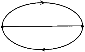One can convince oneself that the minimum degree of a two–loop function is one, and is attained by the vacuum diagram with two fermion propagators and one boson propagator shown in fig. 1. By adding external bosonic lines or pairs of fermionic lines to a diagram one can only increase the degree of the diagram.

Figure 1: Two–loop vacuum diagram with one boson and two fermion propagators, which leads to a ${\cal P}$ function of minimum degree (one). Vacuum diagrams are expressed analytically in terms of Spence functions, but one can obtain nontrivial ${\cal P}$ functions of degree one by adding external bosonic lines to this diagram.

Therefore, by using eqns. 11 and 12 one can derive all functions ${\cal P}^{a\,b}_{\alpha_{1}\,\alpha_{2}\,\alpha_{3}}$ which may appear in renormalizable theories from those with $\alpha_{1}=\alpha_{2}=\alpha_{3}=1$ and $a+b=0,1,2$. Nevertheless, we choose to use the following set instead:

$$\begin{array}[]{lllll}\mbox{degree}=4:&{\cal P}^{0\,0}_{2\,1\,1}&&&\\ \mbox{degree}=3:&{\cal P}^{1\,0}_{2\,1\,1}&{\cal P}^{0\,1}_{2\,1\,1}&&\\ \mbox{degree}=2:&{\cal P}^{2\,0}_{2\,1\,1}&{\cal P}^{1\,1}_{2\,1\,1}&{\cal P}^{0\,2}_{2\,1\,1}&\\ \mbox{degree}=1:&{\cal P}^{3\,0}_{2\,1\,1}&{\cal P}^{2\,1}_{2\,1\,1}&{\cal P}^{1\,2}_{2\,1\,1}&{\cal P}^{0\,3}_{2\,1\,1}\end{array}$$ (14)

The reason is that for these functions one can obtain simpler integral representations than for the functions with $\alpha_{1}=\alpha_{2}=\alpha_{3}=1$. The functions with $\alpha_{1}=\alpha_{2}=\alpha_{3}=1$ are then derived from the set of eq. 14 by using the ”partial $p$” operation of ’t Hooft and Veltman [2].

By applying partial $p$ to ${\cal P}^{a\,b}_{\alpha_{1}\,\alpha_{2}\,\alpha_{3}}$, one finds the following relation:

$${\cal P}^{a\,b}_{\alpha_{1}\,\alpha_{2}\,\alpha_{3}} = -\frac{1}{n-(\alpha_{1}+\alpha_{2}+\alpha_{3})+(a+b)/2}\left\{\alpha_{1}m_{1}^{2}{\cal P}^{a\,b}_{\alpha_{1}+1\,\alpha_{2}\,\alpha_{3}}+\alpha_{2}m_{2}^{2}{\cal P}^{a\,b}_{\alpha_{1}\,\alpha_{2}+1\,\alpha_{3}}\right.$$ (15)

$$\left.\;\;\;\;\;\;\;\;\;\;\;\;\;\;\;\;\;+\alpha_{3}m_{3}^{2}{\cal P}^{a\,b}_{\alpha_{1}\,\alpha_{2}\,\alpha_{3}+1}-\frac{1}{2}\left[2k^{2}\frac{\partial}{\partial k^{2}}-(a+b)\right]{\cal P}^{a\,b}_{\alpha_{1}\,\alpha_{2}\,\alpha_{3}}\right\}\;\;,$$

and this can be used together with eqns. 12 or 13 for expressing the functions with $\alpha_{1}=\alpha_{2}=\alpha_{3}=1$ in terms of the set in eq. 14 when they are needed.

Note that not all functions in eq. 14 are independent. Some of them are related by loop momentum redefinitions. For instance, the following relation holds:

$${\cal P}^{1\,0}_{2\,1\,1}(m_{1},m_{2},m_{3};k^{2})+{\cal P}^{0\,1}_{2\,1\,1}(m_{1},m_{2},m_{3};k^{2})\,=$$ (16)

$$\;\;\;\;\;\;\;\;\;\;\;\;\;\;\;\;\;\;\;\;\;\;\;\;-\left[{\cal P}^{0\,1}_{2\,1\,1}(m_{1},m_{3},m_{2};k^{2})+k^{2}{\cal P}^{0\,0}_{2\,1\,1}(m_{1},m_{3},m_{2};k^{2})\right]\;\;.$$

At the same time, some of these functions may actually never appear directly from a Feynman diagram, as is the case with ${\cal P}^{0\,3}_{2\,1\,1}$. However, they may appear indirectly when using eqns. 12, 13 or 15. For this reason we prefer not to discard them at this point.

The set of functions in eq. 14 is an extension of the functions ${\cal F}$ and ${\cal G}$ of ref. [10]. ${\cal F}$ and ${\cal G}$ are enough for treating all diagrams without numerators. This is the case for instance with the linear sigma model. As already mentioned, the lowest degree which may appear in the linear sigma model is three. Therefore, only the first two lines of eq. 14 are involved. In fact, ${\cal P}^{0\,0}_{2\,1\,1}={\cal G}$, and ${\cal P}^{1\,0}_{2\,1\,1}=-{\cal F}$. The remaining degree three function, ${\cal P}^{0\,1}_{2\,1\,1}$, never appears directly in this case from a Feynman diagram.

One also notices that eq. 15 is a generalization of eq. 11 of ref. [10].

Finally, a remark on nonrenormalizable theories is in order. One can construct two–loop Feynman diagrams of degree lower than one if one allows for nonrenormalizable interactions. As an example, the two–loop sunset self–energy in a four–fermion interaction theory is of degree zero. In nonrenormalizable theories it is not always possible to restrict the degree of the ${\cal P}^{a\,b}_{\alpha_{1}\,\alpha_{2}\,\alpha_{3}}$ functions and thus to identify a finite set of basic functions which generate all the other. In the following section we will derive one–dimensional integral representations for the functions of eq. 14. As it will become clear, it is possible to derive similar integral representations for functions with $a+b>3$ as well. Thus, specific calculations in nonrenormalizable theories can be performed, too. One only needs to introduce additional functions along with those of eq. 14.

4 Integral representations

We have seen in the previous sections that any two–loop Feynman diagram in a renormalizable theory can be expressed in terms of the ten functions of eq. 14, not all of them independent.

As said, our aim here is to express the ultraviolet finite parts of a calculation in a general kinematical situation in a form which would facilitate their numerical evaluation. The reader may know that, already at the level of two–point functions, the self–energy sunset diagram is known to be related to the Lauricella functions [9]. These functions are not straightforward to evaluate numerically. The best way to do that appears to be by means of integral representations [19]. For more complicated two–loop diagrams no analytical results are known so far. Besides, we want to deal with more realistic situations, where non–trivial numerators are present in the integrands.

Hence, in this section we derive one–dimensional integral representations of the ten functions in eq. 14. Such integral representations can be used for a fast and accurate numerical evaluation of these functions.

It is convenient to replace the set of ten functions ${\cal P}^{a\,b}_{2\,1\,1}(m_{1},m_{2},m_{3};k^{2})$ of eq. 14 by the following equivalent set ${\cal H}_{i}(m_{1},m_{2},m_{3};k^{2})$:

$${\cal P}^{0\,0}_{2\,1\,1}\;\rightarrow{\cal H}_{1} = \int d^{n}p\,d^{n}q\,\frac{1}{[(p+k)^{2}+m_{1}^{2}]^{2}\,(q^{2}+m_{2}^{2})\,(r^{2}+m_{3}^{2})}$$

$${\cal P}^{1\,0}_{2\,1\,1}\;\rightarrow{\cal H}_{2} = \int d^{n}p\,d^{n}q\,\frac{p\cdot k}{[(p+k)^{2}+m_{1}^{2}]^{2}\,(q^{2}+m_{2}^{2})\,(r^{2}+m_{3}^{2})}$$

$${\cal P}^{0\,1}_{2\,1\,1}\;\rightarrow{\cal H}_{3} = \int d^{n}p\,d^{n}q\,\frac{q\cdot k}{[(p+k)^{2}+m_{1}^{2}]^{2}\,(q^{2}+m_{2}^{2})\,(r^{2}+m_{3}^{2})}$$

$${\cal P}^{2\,0}_{2\,1\,1}\;\rightarrow{\cal H}_{4} = \int d^{n}p\,d^{n}q\,\frac{(p\cdot k)^{2}-\frac{1}{n}k^{2}p^{2}}{[(p+k)^{2}+m_{1}^{2}]^{2}\,(q^{2}+m_{2}^{2})\,(r^{2}+m_{3}^{2})}$$

$${\cal P}^{1\,1}_{2\,1\,1}\;\rightarrow{\cal H}_{5} = \int d^{n}p\,d^{n}q\,\frac{(p\cdot k)(q\cdot k)-\frac{1}{n}k^{2}(q\cdot p)}{[(p+k)^{2}+m_{1}^{2}]^{2}\,(q^{2}+m_{2}^{2})\,(r^{2}+m_{3}^{2})}$$

$${\cal P}^{0\,2}_{2\,1\,1}\;\rightarrow{\cal H}_{6} = \int d^{n}p\,d^{n}q\,\frac{(q\cdot k)^{2}-\frac{1}{n}k^{2}q^{2}}{[(p+k)^{2}+m_{1}^{2}]^{2}\,(q^{2}+m_{2}^{2})\,(r^{2}+m_{3}^{2})}$$

$${\cal P}^{3\,0}_{2\,1\,1}\;\rightarrow{\cal H}_{7} = \int d^{n}p\,d^{n}q\,\frac{(p\cdot k)^{3}-\frac{3}{n+2}k^{2}p^{2}(p\cdot k)}{[(p+k)^{2}+m_{1}^{2}]^{2}\,(q^{2}+m_{2}^{2})\,(r^{2}+m_{3}^{2})}$$

$${\cal P}^{2\,1}_{2\,1\,1}\;\rightarrow{\cal H}_{8} = \int d^{n}p\,d^{n}q\,\frac{(p\cdot k)^{2}(q\cdot k)-\frac{3}{n+2}k^{2}p^{2}(q\cdot k)}{[(p+k)^{2}+m_{1}^{2}]^{2}\,(q^{2}+m_{2}^{2})\,(r^{2}+m_{3}^{2})}$$

$${\cal P}^{1\,2}_{2\,1\,1}\;\rightarrow{\cal H}_{9} = \int d^{n}p\,d^{n}q\,\frac{(p\cdot k)(q\cdot k)^{2}-\frac{1}{n+2}k^{2}[2(p\cdot q)(q\cdot k)+q^{2}(p\cdot k)]}{[(p+k)^{2}+m_{1}^{2}]^{2}\,(q^{2}+m_{2}^{2})\,(r^{2}+m_{3}^{2})}$$

$${\cal P}^{0\,3}_{2\,1\,1}\;\rightarrow{\cal H}_{10} = \int d^{n}p\,d^{n}q\,\frac{(q\cdot k)^{3}-\frac{3}{n+2}k^{2}q^{2}(q\cdot k)}{[(p+k)^{2}+m_{1}^{2}]^{2}\,(q^{2}+m_{2}^{2})\,(r^{2}+m_{3}^{2})}$$ (17)

For compactness, we omitted in the above formulae the mass and momentum arguments of the functions ${\cal P}^{a\,b}_{2\,1\,1}(m_{1},m_{2},m_{3};k^{2})$ and ${\cal H}_{i}(m_{1},m_{2},m_{3};k^{2})$.

We choose to consider this set of scalar integrals because their ultraviolet behaviour is logarithmic. This is necessary for deriving simple integral representations of their ultraviolet finite parts. It is straightforward to express the ${\cal P}^{a\,b}_{2\,1\,1}$ functions in terms of the ${\cal H}_{i}$ functions. The necessary conversion formulae are listed in Appendix B.

Simple, one-dimensional representations for the functions ${\cal H}_{1}$ and ${\cal H}_{2}$ were found in ref. [10]. As it turns out, it is possible to derive similar integral representations for the other functions, ${\cal H}_{3}$—${\cal H}_{10}$, as well. We discuss some technical details of deriving such integral representations in Appendix C.

By using the methods discussed in Appendix C, one finds the following expressions for the functions ${\cal H}_{i}$ ($\epsilon=n-4$):

$${\cal H}_{1} = \pi^{4}\left[\frac{2}{\epsilon^{2}}-\frac{1}{\epsilon}(1-2\gamma_{m_{1}})-\frac{1}{2}+\frac{\pi^{2}}{12}-\gamma_{m_{1}}+\gamma_{m_{1}}^{2}+h_{1}\right]$$

$${\cal H}_{2} = \pi^{4}k^{2}\left[-\frac{2}{\epsilon^{2}}+\frac{1}{\epsilon}(\frac{1}{2}-2\gamma_{m_{1}})+\frac{13}{8}-\frac{\pi^{2}}{12}+\frac{\gamma_{m_{1}}}{2}-\gamma_{m_{1}}^{2}-h_{2}\right]$$

$${\cal H}_{3} = \pi^{4}k^{2}\left[\frac{1}{\epsilon^{2}}-\frac{1}{\epsilon}(\frac{1}{4}-\gamma_{m_{1}})-\frac{13}{16}+\frac{\pi^{2}}{24}-\frac{\gamma_{m_{1}}}{4}+\frac{\gamma_{m_{1}}^{2}}{2}+h_{3}\right]$$

$${\cal H}_{4} = \pi^{4}(k^{2})^{2}\left[\frac{3}{2\epsilon^{2}}+\frac{1}{\epsilon}\frac{3\gamma_{m_{1}}}{2}-\frac{175}{96}+\frac{\pi^{2}}{16}+\frac{3\gamma_{m_{1}}^{2}}{4}+\frac{3}{4}h_{4}\right]$$

$${\cal H}_{5} = \pi^{4}(k^{2})^{2}\left[-\frac{3}{4\epsilon^{2}}-\frac{1}{\epsilon}\frac{3\gamma_{m_{1}}}{4}+\frac{175}{192}-\frac{\pi^{2}}{32}-\frac{3\gamma_{m_{1}}^{2}}{8}-\frac{3}{4}h_{5}\right]$$

$${\cal H}_{6} = \pi^{4}(k^{2})^{2}\left[\frac{1}{2\epsilon^{2}}-\frac{1}{\epsilon}(\frac{1}{24}-\frac{\gamma_{m_{1}}}{2})-\frac{19}{32}+\frac{\pi^{2}}{48}-\frac{\gamma_{m_{1}}}{24}+\frac{\gamma_{m_{1}}^{2}}{4}+\frac{3}{4}h_{6}\right]$$

$${\cal H}_{7} = \pi^{4}(k^{2})^{3}\left[-\frac{1}{\epsilon^{2}}-\frac{1}{\epsilon}(\frac{5}{24}+\gamma_{m_{1}})+\frac{287}{192}-\frac{\pi^{2}}{24}-\frac{5\gamma_{m_{1}}}{24}-\frac{\gamma_{m_{1}}^{2}}{2}-\frac{1}{2}h_{7}\right]$$

$${\cal H}_{8} = \pi^{4}(k^{2})^{3}\left[\frac{1}{2\epsilon^{2}}+\frac{1}{\epsilon}(\frac{5}{48}+\frac{\gamma_{m_{1}}}{2})-\frac{287}{384}+\frac{\pi^{2}}{48}+\frac{5\gamma_{m_{1}}}{48}+\frac{\gamma_{m_{1}}^{2}}{4}+\frac{1}{2}h_{8}\right]$$

$${\cal H}_{9} = \pi^{4}(k^{2})^{3}\left[-\frac{1}{3\epsilon^{2}}-\frac{1}{\epsilon}(\frac{1}{24}+\frac{\gamma_{m_{1}}}{3})+\frac{95}{192}-\frac{\pi^{2}}{72}-\frac{\gamma_{m_{1}}}{24}-\frac{\gamma_{m_{1}}^{2}}{6}-\frac{1}{2}h_{9}\right]$$

$${\cal H}_{10} = \pi^{4}(k^{2})^{3}\left[\frac{1}{4\epsilon^{2}}+\frac{1}{\epsilon}(\frac{1}{96}+\frac{\gamma_{m_{1}}}{4})-\frac{283}{768}+\frac{\pi^{2}}{96}+\frac{\gamma_{m_{1}}}{96}+\frac{\gamma_{m_{1}}^{2}}{8}+\frac{1}{2}h_{10}\right]\;\;.$$ (18)

Again, to simplify the notations, we omitted in the above formulae the mass and momentum arguments of the functions ${\cal H}_{i}(m_{1},m_{2},m_{3};k^{2})$ and $h_{i}(m_{1},m_{2},m_{3};k^{2})$. $\gamma_{m_{1}}=\gamma+\log{(\pi m_{1}^{2}/\mu_{1}^{2})}$ , where $\gamma=0.577216$ is the Euler constant and $\mu_{1}$ is the ’t Hooft mass. The ultraviolet finite parts $h_{i}(m_{1},m_{2},m_{3};k^{2})$ of the functions ${\cal H}_{i}(m_{1},m_{2},m_{3};k^{2})$ have the following one–dimensional integral representations:

$$h_{1}(m_{1},m_{2},m_{3};k^{2}) = \int_{0}^{1}dx\,\tilde{g}(x)$$

$$h_{2}(m_{1},m_{2},m_{3};k^{2}) = \int_{0}^{1}dx\,[\tilde{g}(x)+\tilde{f_{1}}(x)]$$

$$h_{3}(m_{1},m_{2},m_{3};k^{2}) = \int_{0}^{1}dx\,[\tilde{g}(x)+\tilde{f_{1}}(x)]\,(1-x)$$

$$h_{4}(m_{1},m_{2},m_{3};k^{2}) = \int_{0}^{1}dx\,[\tilde{g}(x)+\tilde{f_{1}}(x)+\tilde{f_{2}}(x)]$$

$$h_{5}(m_{1},m_{2},m_{3};k^{2}) = \int_{0}^{1}dx\,[\tilde{g}(x)+\tilde{f_{1}}(x)+\tilde{f_{2}}(x)]\,(1-x)$$

$$h_{6}(m_{1},m_{2},m_{3};k^{2}) = \int_{0}^{1}dx\,[\tilde{g}(x)+\tilde{f_{1}}(x)+\tilde{f_{2}}(x)]\,(1-x)^{2}$$

$$h_{7}(m_{1},m_{2},m_{3};k^{2}) = \int_{0}^{1}dx\,[\tilde{g}(x)+\tilde{f_{1}}(x)+\tilde{f_{2}}(x)+\tilde{f_{3}}(x)]$$

$$h_{8}(m_{1},m_{2},m_{3};k^{2}) = \int_{0}^{1}dx\,[\tilde{g}(x)+\tilde{f_{1}}(x)+\tilde{f_{2}}(x)+\tilde{f_{3}}(x)]\,(1-x)$$

$$h_{9}(m_{1},m_{2},m_{3};k^{2}) = \int_{0}^{1}dx\,[\tilde{g}(x)+\tilde{f_{1}}(x)+\tilde{f_{2}}(x)+\tilde{f_{3}}(x)]\,(1-x)^{2}$$

$$h_{10}(m_{1},m_{2},m_{3};k^{2}) = \int_{0}^{1}dx\,[\tilde{g}(x)+\tilde{f_{1}}(x)+\tilde{f_{2}}(x)+\tilde{f_{3}}(x)]\,(1-x)^{3}\;\;.$$ (19)

All ten integral representations are built out of the following four basic functions:

$$\tilde{g}(m_{1},m_{2},m_{3};k^{2};x) = Sp(\frac{1}{1-y_{1}})+Sp(\frac{1}{1-y_{2}})+y_{1}\log{\frac{y_{1}}{y_{1}-1}}+y_{2}\log{\frac{y_{2}}{y_{2}-1}}$$

$$\tilde{f_{1}}(m_{1},m_{2},m_{3};k^{2};x) = \frac{1}{2}\left[-\frac{1-\mu^{2}}{\kappa^{2}}+y_{1}^{2}\log{\frac{y_{1}}{y_{1}-1}}+y_{2}^{2}\log{\frac{y_{2}}{y_{2}-1}}\right]$$

$$\tilde{f_{2}}(m_{1},m_{2},m_{3};k^{2};x) = \frac{1}{3}\left[-\frac{2}{\kappa^{2}}-\frac{1-\mu^{2}}{2\kappa^{2}}-\left(\frac{1-\mu^{2}}{\kappa^{2}}\right)^{2}\right.$$

$$\;\;\;\;\;\;\;\;\;\;\;\;\;\;\;\;\;\;\;\;\;\;\;\;\;\;\;\;\;\;\;\;\;\;\;\;\left.+y_{1}^{3}\log{\frac{y_{1}}{y_{1}-1}}+y_{2}^{3}\log{\frac{y_{2}}{y_{2}-1}}\right]$$

$$\tilde{f_{3}}(m_{1},m_{2},m_{3};k^{2};x) = \frac{1}{4}\left[-\frac{4}{\kappa^{2}}-\left(\frac{1}{3}+\frac{3}{\kappa^{2}}\right)\left(\frac{1-\mu^{2}}{\kappa^{2}}\right)-\frac{1}{2}\left(\frac{1-\mu^{2}}{\kappa^{2}}\right)^{2}-\left(\frac{1-\mu^{2}}{\kappa^{2}}\right)^{3}\right.$$ (20)

$$\left.\;\;\;\;\;\;\;\;\;\;\;\;\;\;\;\;\;\;\;\;\;\;\;\;\;\;\;\;\;\;\;\;\;\;\;\;+y_{1}^{4}\log{\frac{y_{1}}{y_{1}-1}}+y_{2}^{4}\log{\frac{y_{2}}{y_{2}-1}}\right]\;\;,$$

where we use the following notations:

$$y_{1,2} = \frac{1+\kappa^{2}-\mu^{2}\pm\sqrt{\Delta}}{2\kappa^{2}}$$

$$\Delta = (1+\kappa^{2}-\mu^{2})^{2}+4\kappa^{2}\mu^{2}-4i\kappa^{2}\eta\;\;,$$ (21)

and

$$\mu^{2} = \frac{ax+b(1-x)}{x(1-x)}$$

$$a = \frac{m_{2}^{2}}{m_{1}^{2}}\,,\;\;\;\;b\;=\;\frac{m_{3}^{2}}{m_{1}^{2}}\,,\;\;\;\;\kappa^{2}\;=\;\frac{k^{2}}{m_{1}^{2}}\;\;.$$ (22)

In the above expressions, one special case must be treated separately, namely $k^{2}=0$. One can convince oneself that in this case our approach reduces to the functions introduced by van der Bij and Veltman in ref. [8].

The functions $\tilde{g}$ and $\tilde{f_{1}}$ were already introduced in ref. [10]. They are sufficient for treating Feynman diagrams without numerators. The other two functions, $\tilde{f_{2}}$ and $\tilde{f_{3}}$, have a similar structure. They are needed for treating functions of degree two and one, respectively, which may appear for instance in a renormalizable theory with fermions. Clearly, it is possible to extend these formulae to functions of lower degree which may appear in nonrenormalizable theories.

In order to calculate more complicated diagrams, the derivatives of the functions defined in eqns. 20 are needed. One may ask oneself whether this procedure does not introduce additional singularities in the integrands, for instance at $x=0,1$. One can convince oneself rather easily that this is not the case. This can be seen by noticing that near x = 0 (the situation is the same at x = 1), the function e.g. $\tilde{g}$, behaves like $\log{x}^{2}$, which is integrable. It is easily seen that by differentiating with respect to one mass or external momentum the behaviour near $x=0$ will remain integrable. By differentiating the function an arbitrary number of times one cannot induce additional singularities in the integral representation. The derivatives will remain integrable. Since there can be no fundamental difficulty related to the differentiation procedure, the problem of evaluating numerically the derivatives is merely a question of implementing the formulae in a computer program in a correct, numerically stable form. This was shown in previous works, e.g. refs. [10, 12], which involve a subset of the $h_{i}$ functions, and where the differentiation procedure was used.

The relations 19 can be used for an efficient numerical evaluation of two–loop Feynman diagrams. We do not enter here into details regarding the numerical integration. Let us just note that this was done in refs. [10]—[12] for $h_{1}$ and $h_{2}$ in the case of two– and three–point functions, and the results agree with independent calculations [13]—[15]. The other $h$ functions have analytical structures similar to $h_{1}$ and $h_{2}$, so that the same numerical algorithms can be used to evaluate them.

5 Conclusions

We presented a method for treating all two–loop diagrams which may appear in a renormalizable theory in a systematic way. Formulae were given which allow one to express any two–loop diagram in terms of a small number of scalar functions. We derived one–dimensional representations of these scalar functions. They are constructed out of four basic functions which have quite simple expressions. These integral representations can be used further for an efficient evaluation of Feynman diagrams.

A useful feature of our approach is that it is suitable for the automatization of two–loop computations. All algebraic manipulations needed to reduce a Feynman diagram to scalar invariants and to express it in terms of the four basic functions which we introduced are algorithmical. They can be encoded in a computer algebra program to treat automatically two–loop Feynman diagrams.

The calculation of a Feynman diagram implies a numerical integration over $h_{i}$ functions or their derivatives. The maximum dimension of this final integration is the number of propagators minus three. Where derivatives of $h_{i}$ functions are needed, they are straightforward to obtain, for instance by using a computer algebra program.

The numerical integrations, the details of which we do not discuss in this paper, are standard. Let us just note that the analytical structure of the functions involved in the integral representations is known [10]. This allows one to identify their singularities, and to define a complex integration path by means of spline functions. Along such a path one can use an adaptative deterministic algorithm for a fast and accurate numerical integration [10, 12].

In this paper we provide only the formulae which are encountered in renormalizable theories. If calculations in nonrenormalizable theories are addressed, new structures may appear. However, they can be dealt with along the same lines, and lead to similar functions. The main difference is that in nonrenormalizable theories it may be impossible to isolate a finite number of two–loop functions from which all other can be derived by differentiation. In this case one would need to consider a specific process and to identify the necessary functions.

Acknowledgement

We would like to thank the High Energy Theory group of Brookhaven National Laboratory for hospitality in the summer of 1996. The work of A.G. is supported by the Deutsche Forschungsgemeinschaft (DFG). Y.P.Y.’s work is partially supported by the U.S. Department of Energy.

Appendix A

We give here the formulae for decomposing a tensor integral $I^{\mu_{1}\cdots\mu_{j^{\prime}}}$ of the type in eq. 5 for the case $j^{\prime}=4$ into scalar invariants.

Apart from a redefinition of the loop momenta $p$ and $q$, there are three possible cases if $j^{\prime}=4$:

$$\int d^{n}p\,d^{n}q\,\frac{p^{\mu_{1}}_{\perp}p^{\mu_{2}}_{\perp}p^{\mu_{3}}_{\perp}p^{\mu_{4}}_{\perp}P(p\cdot k,q\cdot k)}{(p^{2}+m_{1}^{2})^{\alpha_{1}}\,(q^{2}+m_{2}^{2})^{\alpha_{2}}\,[(r+k)^{2}+m_{3}^{2}]^{\alpha_{3}}}\,=$$ (23)

$$C\,\left\{\left(-k^{2}g^{\mu_{1}\mu_{2}}g^{\mu_{3}\mu_{4}}+g^{\mu_{1}\mu_{2}}k^{\mu_{3}}k^{\mu_{4}}+g^{\mu_{3}\mu_{4}}k^{\mu_{1}}k^{\mu_{2}}-\frac{1}{k^{2}}k^{\mu_{1}}k^{\mu_{2}}k^{\mu_{3}}k^{\mu_{4}}\right)\right.$$

$$\left.+\left[(\mu_{1}\mu_{2}\mu_{3}\mu_{4})\leftrightarrow(\mu_{1}\mu_{3}\mu_{2}\mu_{4})\right]+\left[(\mu_{1}\mu_{2}\mu_{3}\mu_{4})\leftrightarrow(\mu_{1}\mu_{4}\mu_{2}\mu_{3})\right]\,\right\}$$

$$\int d^{n}p\,d^{n}q\,\frac{q^{\mu_{1}}_{\perp}p^{\mu_{2}}_{\perp}p^{\mu_{3}}_{\perp}p^{\mu_{4}}_{\perp}P(p\cdot k,q\cdot k)}{(p^{2}+m_{1}^{2})^{\alpha_{1}}\,(q^{2}+m_{2}^{2})^{\alpha_{2}}\,[(r+k)^{2}+m_{3}^{2}]^{\alpha_{3}}}\,=$$ (24)

$$D\,\left\{\left(-k^{2}g^{\mu_{1}\mu_{2}}g^{\mu_{3}\mu_{4}}+g^{\mu_{1}\mu_{2}}k^{\mu_{3}}k^{\mu_{4}}+g^{\mu_{3}\mu_{4}}k^{\mu_{1}}k^{\mu_{2}}-\frac{1}{k^{2}}k^{\mu_{1}}k^{\mu_{2}}k^{\mu_{3}}k^{\mu_{4}}\right)\right.$$

$$\left.+\left[(\mu_{1}\mu_{2}\mu_{3}\mu_{4})\leftrightarrow(\mu_{1}\mu_{3}\mu_{2}\mu_{4})\right]+\left[(\mu_{1}\mu_{2}\mu_{3}\mu_{4})\leftrightarrow(\mu_{1}\mu_{4}\mu_{2}\mu_{3})\right]\,\right\}$$

$$\int d^{n}p\,d^{n}q\,\frac{q^{\mu_{1}}_{\perp}q^{\mu_{2}}_{\perp}p^{\mu_{3}}_{\perp}p^{\mu_{4}}_{\perp}P(p\cdot k,q\cdot k)}{(p^{2}+m_{1}^{2})^{\alpha_{1}}\,(q^{2}+m_{2}^{2})^{\alpha_{2}}\,[(r+k)^{2}+m_{3}^{2}]^{\alpha_{3}}}\,=$$ (25)

$$\left\{E\,\left(-k^{2}g^{\mu_{1}\mu_{2}}g^{\mu_{3}\mu_{4}}+g^{\mu_{1}\mu_{2}}k^{\mu_{3}}k^{\mu_{4}}+g^{\mu_{3}\mu_{4}}k^{\mu_{1}}k^{\mu_{2}}-\frac{1}{k^{2}}k^{\mu_{1}}k^{\mu_{2}}k^{\mu_{3}}k^{\mu_{4}}\right)\right.$$

$$+\left.F\,\left\{\left[(\mu_{1}\mu_{2}\mu_{3}\mu_{4})\leftrightarrow(\mu_{1}\mu_{3}\mu_{2}\mu_{4})\right]+\left[(\mu_{1}\mu_{2}\mu_{3}\mu_{4})\leftrightarrow(\mu_{1}\mu_{4}\mu_{2}\mu_{3})\right]\,\right\}\right\}\;\;,$$

where

$$C = -\frac{1}{(n^{2}-1)k^{2}}\int d^{n}p\,d^{n}q\,\frac{(p_{\perp}^{2})^{2}P(p\cdot k,q\cdot k)}{(p^{2}+m_{1}^{2})^{\alpha_{1}}\,(q^{2}+m_{2}^{2})^{\alpha_{2}}\,[(r+k)^{2}+m_{3}^{2}]^{\alpha_{3}}}$$

$$D = -\frac{1}{(n^{2}-1)k^{2}}\int d^{n}p\,d^{n}q\,\frac{(p_{\perp}\cdot q_{\perp})p_{\perp}^{2}P(p\cdot k,q\cdot k)}{(p^{2}+m_{1}^{2})^{\alpha_{1}}\,(q^{2}+m_{2}^{2})^{\alpha_{2}}\,[(r+k)^{2}+m_{3}^{2}]^{\alpha_{3}}}$$

$$E = -\frac{1}{(n^{2}-1)(n-2)k^{2}}\times$$

$$\;\;\;\;\;\;\;\;\;\;\;\;\;\;\;\;\;\;\;\;\int d^{n}p\,d^{n}q\,\frac{\left[np_{\perp}^{2}q_{\perp}^{2}-2(p_{\perp}\cdot q_{\perp})^{2}\right]P(p\cdot k,q\cdot k)}{(p^{2}+m_{1}^{2})^{\alpha_{1}}\,(q^{2}+m_{2}^{2})^{\alpha_{2}}\,[(r+k)^{2}+m_{3}^{2}]^{\alpha_{3}}}$$

$$F = \frac{1}{(n^{2}-1)(n-2)k^{2}}\times$$ (26)

$$\;\;\;\;\;\;\;\;\;\;\;\;\;\;\;\;\;\;\;\;\int d^{n}p\,d^{n}q\,\frac{\left[p_{\perp}^{2}q_{\perp}^{2}-(n-1)(p_{\perp}\cdot q_{\perp})^{2}\right]P(p\cdot k,q\cdot k)}{(p^{2}+m_{1}^{2})^{\alpha_{1}}\,(q^{2}+m_{2}^{2})^{\alpha_{2}}\,[(r+k)^{2}+m_{3}^{2}]^{\alpha_{3}}}\;\;.$$

The scalar invariants $C$, $D$, $E$ and $F$ can be further reduced to functions of the form of eq. 3 by using the relations:

$$p_{\perp}^{2} = p^{2}-\frac{1}{k^{2}}\,(p\cdot k)^{2}$$

$$p_{\perp}\cdot q_{\perp} = p\cdot q-\frac{1}{k^{2}}\,(p\cdot k)(q\cdot k)$$

$$p\cdot q = \frac{1}{2}\,(r^{2}-p^{2}-q^{2})$$

and by partial fractioning the resulting expressions.

Appendix B

In section 4 we replaced the set of functions ${\cal P}^{a\,b}_{2\,1\,1}$ , $a+b=0,1,2,3$ by the functions ${\cal H}_{1}$—${\cal H}_{10}$. The functions ${\cal H}_{i}$ are free of quadratic divergencies, and for this reason they have simpler integral representations. The relations between ${\cal P}^{a\,b}_{2\,1\,1}$ and ${\cal H}_{i}$ are easily obtained by partial fractioning the eqns. 17:

$${\cal P}^{0\,0}_{2\,1\,1} = {\cal H}_{1}$$

$${\cal P}^{1\,0}_{2\,1\,1} = -{\cal H}_{2}-k^{2}{\cal H}_{1}$$

$${\cal P}^{0\,1}_{2\,1\,1} = -{\cal H}_{3}$$

$${\cal P}^{2\,0}_{2\,1\,1} = {\cal H}_{4}+\frac{k^{2}}{n}\left\{[(n-1)k^{2}-m_{1}^{2}]{\cal H}_{1}+2(n-1){\cal H}_{2}+{\cal P}^{0\,0}_{1\,1\,1}\right\}$$

$${\cal P}^{1\,1}_{2\,1\,1} = {\cal H}_{5}+k^{2}{\cal H}_{3}+\frac{k^{2}}{2n}\left\{(m_{1}^{2}+m_{2}^{2}-m_{3}^{2}+k^{2}){\cal H}_{1}+2{\cal H}_{2}-{\cal P}^{0\,0}_{1\,1\,1}\right.$$

$$\left.\;\;\;\;\;\;\;\;\;\;\;\;\;\;\;\;\;\;\;\;\;\;\;\;\;\;\;\;\;\;\;\;\;\;\;\;\;\;\;\;\;\;\;\;\;\;\;\;\;\;\;\;\;\;\;\;\;\;\;\;\;\;\;\;\;\;\;\;+T_{2}(m_{1}^{2})\left[T_{1}(m_{2}^{2})-T_{1}(m_{3}^{2})\right]\right\}$$

$${\cal P}^{0\,2}_{2\,1\,1} = {\cal H}_{6}+\frac{k^{2}}{n}\left[-m_{2}^{2}{\cal H}_{1}+T_{2}(m_{1}^{2})T_{1}(m_{3}^{2})\right]$$

$${\cal P}^{3\,0}_{2\,1\,1} = -{\cal H}_{7}-\frac{3k^{2}}{n+2}\left\{\left(\frac{n-1}{3}k^{2}-m_{1}^{2}\right)k^{2}{\cal H}_{1}+[(n-1)k^{2}-m_{1}^{2}]{\cal H}_{2}+n{\cal H}_{4}-{\cal P}^{1\,0}_{1\,1\,1}\right\}$$

$${\cal P}^{2\,1}_{2\,1\,1} = -{\cal H}_{8}-\frac{3k^{2}}{n+2}\left[\frac{2}{3}(n-1){\cal H}_{5}+\left(\frac{n-1}{3}k^{2}-m_{1}^{2}\right){\cal H}_{3}-{\cal P}^{0\,1}_{1\,1\,1}\right]-\frac{n-1}{n(n+2)}(k^{2})^{2}$$

$$\times\left\{(m_{1}^{2}+m_{2}^{2}-m_{3}^{2}+k^{2}){\cal H}_{1}+2{\cal H}_{2}-{\cal P}^{0\,0}_{1\,1\,1}+T_{2}(m_{1}^{2})[T_{1}(m_{2}^{2})-T_{1}(m_{3}^{2})]\right\}$$

$${\cal P}^{1\,2}_{2\,1\,1} = -{\cal H}_{9}-k^{2}{\cal H}_{6}-\frac{k^{2}}{n+2}\left[2{\cal H}_{5}+(\frac{2k^{2}}{n}-m_{2}^{2}){\cal H}_{2}+(m_{1}^{2}+m_{2}^{2}-m_{3}^{2}+k^{2}){\cal H}_{3}+{\cal P}^{0\,1}_{1\,1\,1}\right]$$

$$-\frac{(k^{2})^{2}}{n(n+2)}\left\{(m_{1}^{2}-(n+1)m_{2}^{2}-m_{3}^{2}+k^{2}){\cal H}_{1}-{\cal P}^{0\,0}_{1\,1\,1}\right.$$

$$\left.\;\;\;\;\;\;\;\;\;\;\;\;\;\;\;\;\;\;\;\;\;\;\;\;\;\;\;\;\;\;\;\;\;\;\;\;\;\;\;\;\;\;\;\;\;\;\;\;\;\;\;\;\;\;\;\;\;\;+T_{2}(m_{1}^{2})[T_{1}(m_{2}^{2})-(n-1)T_{1}(m_{3}^{2})]\right\}$$

$${\cal P}^{0\,3}_{2\,1\,1} = -{\cal H}_{10}-\frac{3k^{2}}{n+2}\left[-m_{2}^{2}{\cal H}_{3}+k^{2}T_{2}(m_{1}^{2})T_{1}(m_{3}^{2})\right]\;\;\;\;,$$ (27)

where $T_{1}$ and $T_{2}$ are the Euclidian one–loop tadpole integrals:

$$T_{1}(m^{2}) = \int d^{n}p\,\frac{1}{p^{2}+m^{2}}\;=\;-\pi^{2}\left(\pi m^{2}\right)^{\frac{\epsilon}{2}}\Gamma\left(-\frac{\epsilon}{2}\right)\,\frac{2m^{2}}{2+\epsilon}$$

$$T_{2}(m^{2}) = \int d^{n}p\,\frac{1}{(p^{2}+m^{2})^{2}}\;=\;\pi^{2}\left(\pi m^{2}\right)^{\frac{\epsilon}{2}}\Gamma\left(-\frac{\epsilon}{2}\right)\;\;.$$ (28)

For simplifying the notation, we omitted in the above formulae the mass and momentum arguments of the functions ${\cal H}_{i}(m_{1},m_{2},m_{3};k^{2})$ and ${\cal P}^{a\,b}_{\alpha_{1}\,\alpha_{2}\,\alpha_{3}}(m_{1},m_{2},m_{3};k^{2})$, and understand that these arguments appear in this order in all relations.

The functions with $\alpha_{1}=\alpha_{2}=\alpha_{3}=1$ which appear in the relations 27 can be calculated by partial $p$ (eq. 15):

$${\cal P}^{1\,0}_{1\,1\,1}(m_{1},m_{2},m_{3};k^{2}) = -\frac{1}{n-\frac{5}{2}}\left\{\left[\frac{k^{2}}{2}{\cal P}^{0\,0}_{1\,1\,1}-{\cal P}^{2\,0}_{2\,1\,1}-m_{1}^{2}({\cal H}_{2}+k^{2}{\cal H}_{1})\right](m_{1},m_{2},m_{3};k^{2})\right.$$

$$\left.-m_{2}^{2}{\cal H}_{3}(m_{2},m_{1},m_{3};k^{2})+m_{3}^{2}({\cal H}_{2}+{\cal H}_{3})(m_{3},m_{2},m_{1};k^{2})\right\}$$

$${\cal P}^{0\,0}_{1\,1\,1}(m_{1},m_{2},m_{3};k^{2}) = -\frac{1}{n-3}\left\{\left[(m_{1}^{2}+k^{2}){\cal H}_{1}+{\cal H}_{2}\right](m_{1},m_{2},m_{3};k^{2})\right.$$ (29)

$$\;\;\;\;\;\;\;\;\;\;\left.+m_{2}^{2}{\cal H}_{1}(m_{2},m_{1},m_{3};k^{2})+m_{3}^{2}{\cal H}_{1}(m_{3},m_{1},m_{2};k^{2})\right\}$$

Appendix C

Here we make some comments on the derivation of the integral representations of the functions ${\cal H}_{i}$. The derivation proceeds in the same way for all ten functions, and works for functions of lower degree as well.

Let us consider for instance the function ${\cal H}_{6}$:

$${\cal H}_{6}(m_{1},m_{2},m_{3};k^{2})=\int d^{n}p\,d^{n}q\,\frac{(q\cdot k)^{2}-\frac{1}{n}k^{2}q^{2}}{[(p+k)^{2}+m_{1}^{2}]^{2}\,(q^{2}+m_{2}^{2})\,(r^{2}+m_{3}^{2})}$$ (30)

We introduce two Feynman parameters $x$ and $y$, and integrate out the loop momenta $p$ and $q$. Note that the quadratic divergence which is present in the ${\cal P}^{0\,2}_{2\,1\,1}$ integral cancels out in ${\cal H}_{6}$. This is necessary for obtaining a well–defined integral representation of the ultraviolet finite part. Without this cancellation, part of the ultraviolet divergence of the diagram is transferred from the radial loop momenta integration to the Feynman parameters integration; one is then left with a nonintegrable singularity in the $x$ integration.

After integrating out the $q$ and $p$ loop momenta, one finds ($n=4+\epsilon$):

$${\cal H}_{6}(m_{1},m_{2},m_{3};k^{2}) = \pi^{4}(k^{2})^{2}\Gamma\left(-\frac{\epsilon}{2}\right)\Gamma(-\epsilon)\frac{1-\frac{1}{n}}{\Gamma\left(3-\frac{n}{2}\right)}\left(\pi m_{1}^{2}\right)^{\epsilon}$$ (31)

$$\times\int_{0}^{1}dx\,[x(1-x)]^{\frac{\epsilon}{2}}(1-x)^{2}$$

$$\times\int_{0}^{1}dy\,\left[\frac{R^{2}}{1-y}\right]^{\frac{\epsilon}{2}}\left[4+\frac{\epsilon}{2}\left(1-2\frac{L}{R}\right)\right]y^{3}\;\;\;.$$

Here we introduced the following notation in addition to eqns. 21 and 22:

$$L = y^{2}\kappa^{2}+\mu^{2}$$

$$R = y(1-y)\kappa^{2}+y+(1-y)\mu^{2}\;\equiv\;\kappa^{2}(y_{1}-y)(y-y_{2})$$ (32)

Eq. 31 displays already the structure of the function ${\cal H}_{6}$. The first line of eq. 31 contains the ultraviolet singularity, while the $y$ and $x$ integrals are finite. Hence, the $x$ and $y$ integrations need to be performed up to ${\cal O}(\epsilon^{2})$. Therefore, one expands the integrand in powers of $\epsilon$ up to order ${\cal O}(\epsilon^{2})$ and carries out the $y$ integration. The calculation can be simplified considerably by using the relation:

$$\frac{L}{R}=1-\frac{y}{R}\frac{\partial R}{\partial y}\;\;\;.$$ (33)

Finally, one obtains after the $y$ integration the results given in eqns. 18—20.