ANL-HEP-PR-96-103 hep-ph/97xxyyy

Probing Nucleon Spin Structure

Gordon P. Ramsey

Physics Department, Loyola University of Chicago, Chicago, IL 60626

and

High Energy Physics Division, Argonne National Laboratory, IL 60439

One of the important questions in high energy physics is the relation of quark and gluon spin to that of the nucleons which they comprise. Polarization experiments provide a mechanism to probe the spin properties of elementary particles and provide crucial tests of Quantum Chromodynamics (QCD). The theoretical and experimental status of this fundamental question will be reviewed in this paper.

1 INTRODUCTION

1.1 Motivation for Spin Studies

In recent years there has been a significant interest in the study of spin phenomena. It is now widely accepted that the physics of spin phenomena in particle interactions provides vital information on the most profound properties of particles: their wave functions, the short and long distance dynamics of the quark and gluon interactions, and the mechanisms of chiral symmetry breaking and confinement. These systematic spin studies have several well defined goals; some of these include:

• The study of the spin structure of the nucleon, i.e., how the proton’s spin state can be obtained from a superposition of Fock states with different numbers of constituents with spin.

• How the dynamics of constituent interactions depend on spin.

• Study the overall nucleon structure and long range dynamics.

• Understand chiral symmetry breaking and helicity non-conservation on the hadronic level.

The first two goals are related to the constituent short-interaction dynamics, while the last two concentrate on hadronic long-range (non-perturbative) dynamics. Experiments designed to investigate all of these important properties of nucleons can be performed with polarized proton beams at many present accelerators. These experiments can also be used to test some fundamental assumptions of QCD regarding spin.

The naive quark model has been successful in predicting most of the gross properties of hadrons, such as charge, parity, isospin and symmetry properties in relation to each other. Some of the dynamics of particle interactions can qualitatively be understood in terms of this model, as well. However, it has been noted, within the past decade, that it falls short in explaining the spin properties of hadrons in terms of their constituents. Perturbative QCD (PQCD) has also been successful in predicting asymptotic properties of hadronic dynamics in the limit of short range interactions. Once again, some of the PQCD predictions regarding spin have disagreed with data, even in those kinematic regions where PQCD is thought to be valid. The data include measurements of analyzing power, which yielded non-zero values, in contrast to PQCD predictions and oscillations in exclusive $p-p$ scattering cross sections. These are related to the assumption of helicity conservation on the hadronic level. Hyperon production experiments from inclusive $p-p$ scattering have shown that polarized hyperons can be produced from unpolarized protons. This is totally unexpected from PQCD arguments and the assumption of the pointlike constituent dynamics. These phenomena are likely related to longer range dynamics and the coordinated rotation of constituents in terms of angular momentum.

Thus, in probing hadronic structure with regard to spin, a number of interesting events have arisen, which require modification of the models created to explain hadronic matter. Outside of new particle discoveries, spin phenomena have provided the high energy community with a great number of surprises, which have forced us to refine our picture of elementary matter.

In this review, I will discuss a particular aspect of this exciting field, namely the quest for understanding nucleon spin with regard to the quark and gluon constituents and their overall collective motion. Naturally, there is some overlap in the understanding of the constituent spin and the overall nucleon spin, since the constituents must be confined to the nucleon “bag”. Also, since the collective motion of the constituents plays and important role in structure and the dynamics of the interactions, some of the analyses will include the non-perturbative effects which are characteristic of the long range dynamics. The main thrust of this paper, however, is to describe the theoretical and experimental aspects of understanding the constituent structure of nucleon spin in fair detail.

1.2 The Spin Crisis

Consituent spin structure studies involve inclusive processes such as the deep inelastic scattering (DIS) of leptons on nucleons. There are two crucial reasons why deep-inelastic scattering is the primary tool for probing hadronic structure: (1) the pointlike nature of the leptons allows the probing of hadrons so that constituent interactions can be ignored, and (2) the theoretically calculable quantities which characterize the constituent structure can be directly related to the measurable cross sections. In other words, the cross sections are factorizable into a calculable part and a measured part. Historically, the deep-inelastic scattering of electrons first proved the existence of point-like constituents in the nucleon. The first spin structure measurements of the proton were performed in the 1970’s when the SLAC-Yale collaboration measured the spin structure function $g_{1}(x)$. [1] In the late 1980’s, the European Muon Collaboration at CERN [2] extended the kinematic range of the DIS measurements using a polarized muon beam. The extrapolation of the polarized structure function $g_{1}^{p}$ to lower $x$ (parton fractional momentum) led to implications that, although the Bjorken sum rule of QCD [3] was satisfied, the Ellis-Jaffe sum rule, [4] based on a simple quark model with unpolarized strange quarks, was violated. This created a controversy, labeled the “spin crisis” which heightened the interest in spin phenomena. Since then, a flurry of theoretical and experimental work has been performed to address this “crisis” and further investigate the spin properties of the lighter hadrons.

Initial analyses of the EMC data were motivated by comparison to the naive quark model and the Ellis-Jaffe sum rule. This sum rule was based on the assumption of an unpolarized strange sea, motivated by unitarity arguments, and will be discussed in detail later. The “spin-crisis” arose since the data disagreed considerably with the naive quark model, which predicted that all of the nucleon spin should be carried by the valence quarks, and the Ellis-Jaffe sum rule. The EMC data led to the implications that:

• (1) the total quark content of the proton spin is small and possibly consistent with zero,
  

• (2) the predictions of the E-J sum rule are severely violated.

There were a number of proposed “fixes” for these problems. [5] Among them were:

• (1) introduction of the gluon anomaly, which can modify the spin content of each quark flavor, so that the measured and calculated values differ by a calculable factor,
  

• (2) proposing that the spin carried by the polarized gluons was extremely large ($\left\langle\Delta G\right\rangle\approx 6$),
  

• (3) assuming that the corresponding orbital motion of the constituents was very large,
  

• (4) assuming that the polarized sea was large and negative, canceling most of the valence quark contribution to the spin,
  

• (5) abandonment of the quark model in favor of alternatives, such as the Skyrme model.

All of these were motivated by the prevailing notion that the naive quark model with an unpolarized strange sea was an accurate model of the nucleons’ spins. Analyses of the more recent data (from 1992 on) are more inclined to accept the notion that the naive quark model must be modified to account for spin contributions of the constituents and that the sea is polarized negatively with respect to the valence quarks. This virtually eliminates the necessity of making the polarized gluons or the angular momentum extremely large. There may be other considerations which affect these quantities in the opposite way, such as negatively polarized gluons and the possibility of rapidly growing structure functions at small $x$. Thus, in response to the recent DIS data, previling theories have reduced the possible range of values of the constituents’ spin contributions and have made us reconsider the important elements which modify these contributions.

Recently, much attention of the HEP community has focused on the physics of polarized hadron interactions. In the last couple of years, experimental groups at SLAC, CERN and DESY have improved statistics and lowered the systematic errors in these DIS experiments. [6, 7, 8] This data has allowed us to draw several conclusions about the nucleon spin structure in the kinematic region of lepton momentum transfer, $Q^{2}\simeq 2\to 10$ GeV² and Bjorken $x\simeq 0.002\to 0.7$. The analysis of these data in the framework of perturbative QCD provides information on longitudinally polarized parton distributions $\Delta q_{i}(x,Q^{2})$, interpreted as the differences of probabilities $q^{+/-}(x,Q^{2})$ for finding partons of the type $i$ with spin parallel/antiparallel to the spin of the parent nucleon. The results have required modification of the earlier quark models of nucleon spin and have created other controversies regarding the amount of spin carried by the strange sea quarks and the gluons. [9] Thus, although there has been significant progress in understanding nucleon spin structure, present data have left unanswered questions regarding: (1) flavor dependent spin structure, (2) relations between the polarized and unpolarized quark and gluon structure functions and (3) choice of factorization of the quark distributions and the role of the gluon anomaly in their determination.

Recently, the E704 group at Fermilab has analyzed the data from their $pp$ and $p\bar{p}$ experiments for jet production cross sections. [10] The results have implied that the polarized gluon distribution is limited in size, but has not put a strict value on this limit. In all of the inclusive experiments done this far, we have gained some knowledge of the constituent spin content, but it is clear that much more work has to be done in future experiments to obtain a complete understanding of this important problem in physics. Since the initial studies of constituent spin structure have relied heavily upon deep-inelastic scattering experiments, it is useful to outline the connection between theoretical calculations and the measured cross sections.

1.3 Deep-Inelastic Scattering

1.3.1 Formalism

Since the pointlike lepton is incident on the hadron target at very high energy, it effectively strikes one of the quarks within the hadron. From the angular distribution of the scattered lepton, the momentum information can be inferred. The polarized deep-inelastic scattering process (DIS) can be represented by the diagram in Fig. 1.

Figure 1: Diagram of Deep-Inelastic Scattering, showing relavent momenta.

In this figure, the initial proton (or hadron target) and lepton $4-$momenta are given by $p^{\mu}$ and $k^{\mu}$, respectively. The virtual exchanged photon has momentum $q$ and the outgoing struck quark and lepton momenta are $p_{x}^{\mu}$ and $k^{\mu\prime}$, respectively. The cross sections are usually written in terms of the invariants: $Q^{2}=-q^{2}$, $\nu=E-E^{\prime}$ and $x=Q^{2}/(2M\nu)$. Here, $Q^{2}$ is the momentum (squared) transfered to the nucleon by the lepton, $\nu$ is the energy lost by the lepton in the collision and thus transferred by the photon to the quark, and $x$ is a dimensionless variable, called the Bjorken scaling variable, which is a measure of the fraction of momentum carried off by the struck quark. [11] Cross section information and the corresponding theoretically generated structure functions are represented in terms of either the variables $\nu$ and $Q^{2}$ or $x$ and $Q^{2}$.

Let us briefly review the formalism of deep inelastic polarized electron scattering on a polarized proton. [12] Since the thrust of this review is to study nucleon spin structure via the constituents, we will cover only the distribution part of the interaction, which involves the structure functions. The final-state fragmentation functions are not considered here, but the reader can refer to recent treatments of spin measurements of the fragmentation functions done by Anselmino, et. al., [13] and Mulders. [14]

In the distribution function case, the hadronic tensor carries all of the relavent information about the target nucleon. This tensor, labeled $W_{\mu\nu}$, will depend on the momenta $p$ and $q$ and on the covariant pseudovector of the proton spin, $s$. Taking into account translation invariance, the hadronic tensor can be rewritten as a Fourier transformation of the matrix element of the commutator of two currents representing the dynamics of the interaction:

$$W_{\mu\nu}(p,q,s)=\frac{1}{4M}\int\frac{d^{4}\xi}{2\pi}\>e^{iq\xi}\langle p,s|[J_{\mu}(\xi),J_{\nu}(0)]|p,s\rangle=W_{\mu\nu}^{[S]}+iW_{\mu\nu}^{[A]},$$ (1)

where $|p,s\rangle$ denotes the proton state with momentum $p$ and spin $s$. The hadronic tensor contains all of the appropriate information necessary to extract the spin-averaged (unpolarized) and spin-weighted (polarized) structure functions in inclusive scattering. For the purpose of separating the unpolarized and polarized information, we can separate the symmetric [S] and anti-symmetric [A] parts of the hadronic tensor. The functions $W_{\mu\nu}^{[S]}$ and $W_{\mu\nu}^{[A]}$ are determined by the discontinuity of the symmetric and antisymmetric parts of the forward Compton scattering amplitude: $W_{\mu\nu}^{[S,A]}=\frac{1}{\pi}\mbox{Im}\>T_{\mu\nu}^{[S,A]}$. Imposing parity (P), charge conjugation (C) and current conservation ($q^{\mu}W_{\mu\nu}=0$) we can extract the forms:

$$W_{\mu\nu}^{[S]}=(-g_{\mu\nu}-{{q_{\mu}q_{\nu}}\over{Q^{2}}})W_{1}(x,Q^{2})+\frac{1}{M^{2}}(p_{\mu}+{{p\cdot q}\over{Q^{2}}}q_{\mu})(p_{\nu}+{{p\cdot q}\over{Q^{2}}}q_{\nu})W_{2}(x,Q^{2})$$ (2)

and

$$W_{\mu\nu}^{[A]}=\frac{1}{M^{4}}\varepsilon_{\mu\nu\lambda\sigma}q^{\lambda}[M^{2}s^{\sigma}G_{1}(\nu,Q^{2})+(Mp\cdot qs^{\sigma}-s\cdot qp^{\sigma})G_{2}(\nu,Q^{2})].$$ (3)

This last relation provides the opportunity to apply the helicity amplitude formalism which is especially useful in the case of targets with spins greater than $1\over 2$. For a spin-$1\over 2$ target there are only four independent helicity amplitudes in forward Compton scattering and hence four independent structure functions. The spin-dependent structure functions $G_{1}$ and $G_{2}$ determine the asymmetries which depend on the initial state lepton and nucleon polarizations.

In the Bjorken limit ($\nu$ and $Q^{2}$ $\to\infty$, $x$ constant) scaling is valid and the functions $W_{1}$, $W_{2}$, $G_{1}$ and $G_{2}$ should depend only on $x$, up to the logarithmic corrections:

$$MW_{1}(\nu,Q^{2})\rightarrow F_{1}(x),$$

$$\nu W_{2}(\nu,Q^{2})\rightarrow F_{2}(x),$$

$$M^{2}\nu G_{1}(\nu,Q^{2})\rightarrow g_{1}(x),$$

$$M\nu^{2}G_{2}(\nu,Q^{2})\rightarrow g_{2}(x).$$ (4)

Studies of deep inelastic scattering processes in the Bjorken scaling limit provide us with the knowledge on the structure of the target nucleon. In the Bjorken scaling limit, the symmetric and anti-symmetric parts of the hadronic tensor are:

$$W_{\mu\nu}^{[S]}=\frac{1}{M}(-g_{\mu\nu}+{{q_{\mu}q_{\nu}}\over{q^{2}}})F_{1}(x,Q^{2})+\frac{1}{M^{2}\nu}(p_{\mu}+{{p\cdot q}\over{Q^{2}}}q_{\mu})(p_{\nu}+{{p\cdot q}\over{Q^{2}}}q_{\nu})F_{2}(x,Q^{2})$$

$$W_{\mu\nu}^{[A]}={{\varepsilon_{\mu\nu\lambda\sigma}q^{\lambda}s^{\sigma}}\over{M^{4}\nu}}g_{1}(x,Q^{2})+{{\varepsilon_{\mu\nu\lambda\sigma}(M\nu s^{\sigma}-q\cdot sp^{\sigma}})\over{M\nu^{2}}}g_{2}(x,Q^{2}).$$ (5)

The functions $F_{1}$ and $F_{2}$ are the structure functions extracted from unpolarized DIS, while $g_{1}$ and $g_{2}$ are extracted from polarized DIS. These reveal the pointlike interaction between the hard photon and the constituent partons within the hadron.

In the operator product expansion of QCD, the local operators are quark and gluon operators, characterized by definite values of twist. The hadronic electromagnetic current in the quark model has the form:

$$J_{\mu}(\xi)=\sum_{q}e_{q}^{2}\bar{q}(\xi)\gamma_{\mu}q(\xi).$$ (6)

Here $q(\xi)$ denotes the quark field. The matrix element between the free quark states is

$$\langle q|JJ|q\rangle\sim c_{q}\langle q|O_{q}|q\rangle+c_{g}\langle q|O_{g}|q\rangle,$$ (7)

where indices $q$ and $g$ refer to the quark and gluon operators. Since the electromagnetic current is a quark operator the left hand side and first term in the right hand side are of order $(\alpha_{s})^{0}$, whereas the matrix element $\langle q|O_{g}|q\rangle$ is of order $(\alpha_{s})^{1}$, because there are at least two gluons entering the operator $O_{g}$. Thus, in general one can neglect the gluon operator. The most important operators in OPE are the operators with the lowest possible twist. The twist-two operators correspond to the vector and axial vector currents for the process of the virtual Compton scattering which determine the hadronic tensor $W_{\mu\nu}$. These operators provide the finite contribution to the structure functions in the deep inelastic limit while the contribution of twist-three operators are suppressed by $M/Q$. Transverse spin structure functions, for example, are of the twist-three type.

The structure function $g_{1}(x,Q^{2})$ is related to the longitudinal polarization of the proton spin with respect to its momentum, i.e. its helicity. In the parton model, $g_{1}$ effectively measures the quark helicity density. The second spin-dependent proton structure function $g_{2}(x,Q^{2})$ is related to transverse polarization of the nucleon spin. It has been measured at SLAC (E143) in a limited $x$ region. The analysis based on the OPE does not depend on the type of nucleon polarization (longitudinal or transverse). The analysis of the second structure function $g_{2}(x,Q^{2})$ may be performed similar to the function $g_{1}(x,Q^{2})$. The significant difference between the two cases is that $g_{1}(x,Q^{2})$ receives a contribution only from twist-two operators whereas $g_{2}(x,Q^{2})$ gets contributions from both twist-two and twist-three operators simultaneously. A few theoretical results have been obtained for the function $g_{2}(x)$, but simple partonic interpretation is only possible for the twist-two operator contribution. The twist-three contributions are not well understood. The following relation exists between the functions $g_{1}$ and the twist-two contribution to $g_{2}$: [15]

$$g_{2}(x,Q^{2})=\int_{x}^{1}\frac{dy}{y}g_{1}(y,Q^{2})-g_{1}(x,Q^{2}).$$ (8)

The above relation is used to calculate $g_{2}(x,Q^{2})$ from $g_{1}(x^{\prime},Q^{2})$ at $x^{\prime}\geq x$ in the framework of the parton model with free on-shell partons. However there are no reasons to neglect the contributions of twist-three operators at low enough $Q^{2}$ and therefore $g_{2}$ can be represented as follows:

$$g_{2}(x,Q^{2})=g_{2}(x,Q^{2})^{[2]}+g_{2}(x,Q^{2})^{[3]},$$ (9)

where the first term on the right hand side of Eqn. (9) is provided by Eqn. (8). The twist-three operator contributions $g_{2}(x,Q^{2})^{[3]}$ depend on the effects of quark-gluon interactions and quark masses.

Experimental measurements of $g_{2}(x,Q^{2})$ provide a direct way to study the magnitude of twist-3 contributions and accurate data with polarized proton beams would be crucial in the resolving of the question of the magnitude of these contributions. Data could also provide a test for the Burkhardt-Cottingham sum rule: [16]

$$\int_{0}^{1}g_{2}(x)=0.$$ (10)

The success or failure of Eq. 1.10 depends on its long-range behavior which, in the simple models, is such that this sum rule is satisfied in perturbative QCD. Thus, valuable information regarding both perturbative and non-perturbative processes can be obtained by testing this sum rule. Recent measurements of $g_{2}$ by the SMC [6] and E143 [17] experiments have verified the condition that $A_{2}<\surd R$ ($R\equiv\sigma_{L}/\sigma_{T}$) so that the leading twist terms dominate and that the Burkhardt-Cottingham sum rule is valid to within experimental errors. There are a number of recent treatments of the role of $g_{2}$ in DIS with regard to transverse spin content and chiral symmetry breaking. [18] This topic will not be discussed here.

The above discussion has shown how the hadronic tensor can be written in terms of the spin-averaged (unpolarized) structure functions $F_{1}$ and $F_{2}$, and the spin-weighted (polarized) structure functions $g_{1}$, $g_{2}$. It is these quantities which can be extracted from the cross sections in various DIS processes. The phenomenology of DIS starts with combining the incident lepton tensor with the hadronic tensor and relating this product to the measured cross sections.

1.3.2 Phenomenology

The polarized lepton tensor $L_{\mu\nu}$, being pointlike, can be written explicitly as:

$$L_{\mu\nu}=2\Bigl{[}k_{\mu}k^{\prime}_{\nu}+k^{\prime}_{\mu}k_{\nu}-g_{\mu\nu}k\cdot k^{\prime}-m_{\mu}^{2})+i\varepsilon_{\mu\nu\rho\sigma}q^{\rho}s^{\sigma}\Bigr{]},$$ (11)

where the antisymmetric last term is absent in the unpolarized case. The product of $L_{\mu\nu}$ and $W_{\mu\nu}$ is directly related to the cross sections measured in the process of DIS.

Since cross sections are the most fundamental measured property of elementary particles, all of the theoretical quantities characterizing spin must be extracted from some combination of the polarization cross sections. [12] The following differential cross section relates to the lepton and hadron tensor product as:

$${{d^{2}\sigma}\over{d\nu dQ^{2}}}={{4\pi\alpha M^{2}}\over{(s-M^{2})^{2}\>Q^{4}}}\cdot L_{\mu\nu}W^{\mu\nu}.$$ (12)

This connects the structure functions in the Bjorken limit directly to the measured cross sections, both in the unpolarized and polarized cases. These differential cross sections can be written as in terms of any of the kinematic variables. For example, if the energies and angular distributions of the leptons are measured, the unpolarized and polarized structure functions are related to the spin averaged and spin weighted differential cross sections by:

$${{d^{2}\sigma(\rightarrow\rightarrow)}\over{d\Omega dE^{\prime}}}+{{d^{2}\sigma(\leftarrow\rightarrow)}\over{d\Omega dE^{\prime}}}={{8\alpha^{2}E^{\prime 2}}\over{MQ^{4}}}\Bigl{[}2\sin^{2}(\theta/2)F_{1}(x,Q^{2})+(M^{2}/\nu)\cos^{2}(\theta/2)F_{2}(x,Q^{2})\Bigr{]},$$ (13)

and

$${{d^{2}\sigma(\rightarrow\rightarrow)}\over{d\Omega dE^{\prime}}}-{{d^{2}\sigma(\leftarrow\rightarrow)}\over{d\Omega dE^{\prime}}}={{4\alpha^{2}E^{\prime}}\over{Q^{2}E\nu}}\Bigl{[}(E+E^{\prime}\cos\bigl{(}\theta)\bigr{)}g_{1}(x,Q^{2})-(2xM)g_{2}(x,Q^{2})\Bigr{]},$$ (14)

where $d\Omega$ is the angular distribution of the leptons.

In nature, asymmetric behavior often occurs between the interactions of particles whose spins are aligned and interactions of particles whose spins are anti-aligned. Thus, it is convenient to define an asymmetry as:

$$A=\Biggl{[}{{\sigma(++)-\sigma(+-)}\over{\sigma(++)+\sigma(+-)}}\Biggr{]},$$

where the ++ refers to the aligned spins and $+-$ to the anti-aligned spins, without regard to the direction of polarization relative to the momentum of the interaction. There are distinct advantages to defining the asymmetries in this way. Theoretically, $A$ is a ratio of cross sections, so all of the normalizations used to calculate cross sections cancel, leaving only the key parameters of the interaction. Experimentally, the difference in the numerator tends to cancel some of the systematic errors, making $A$ a fundamentally more sensitive measure of the physical variables.

There are asymmetries for both the longitudinal and transverse spin relative polarizations. The lepton-hadron asymmetries are given in terms of the cross-section as:

$$A_{\parallel}(x,Q^{2})=\Biggl{[}{{\sigma(\leftarrow\rightarrow)-\sigma(\leftarrow\leftarrow)}\over{\sigma(\leftarrow\rightarrow)+\sigma(\leftarrow\leftarrow)}}\Biggr{]}\equiv\biggl{[}{{\Delta\sigma_{parallel}}\over{\sigma}}\biggr{]}$$

$$A_{\perp}(x,Q^{2})=\Biggl{[}{{\sigma(\uparrow\downarrow)-\sigma(\uparrow\uparrow)}\over{\sigma(\uparrow\downarrow)+\sigma(\uparrow\uparrow)}}\Biggr{]}\equiv\biggl{[}{{\Delta\sigma_{perp}}\over{\sigma}}\biggr{]},$$ (15)

where the arrows refer to the relative longitudinal spin directions of the beam and target, respectively.

The structure functions can be related to the absorptive cross sections, $\sigma_{1\over 2}$ and $\sigma_{3\over 2}$ for virtual photons with helicity projections $1\over 2$ and $3\over 2$, respectively. The asymmetry components $A_{1}$ and $A_{2}$ can be written in terms of the corresponding cross sections along with the interference between the longitudinal and transverse polarizations, $\sigma_{I}$. The parallel asymmetry in terms of these components can be written as

$$A_{\parallel}=D(A_{1}+\eta A_{2}),$$

$$=D\Bigl{[}{{\sigma_{1\over 2}-\sigma_{3\over 2}}\over{\sigma_{1\over 2}+\sigma_{3\over 2}}}\Bigr{]}+2D\eta{{\sigma_{I}}\over{\sigma_{1\over 2}+\sigma_{3\over 2}}}.$$ (16)

The kinematic factors are: $D={{1-(1-y)\epsilon}\over{1+\epsilon R}}$ and $\eta={{2M\epsilon(Q^{2})^{1\over 2}}\over{s[1-(1-y)\epsilon]}}$, where $y$ is the fraction of energy lost be the lepton in the lab frame and $R=\sigma_{L}/\sigma_{T}$, the ratio of transverse to longitudinal photon-nucleon ($\gamma-N$) cross sections. In most DIS experiments, the kinematics are such that $D$ is known for each experiment and $\eta\sim\epsilon Q/s$ is very small. The asymmetries can be linked to the structure functions $g_{1}$ and $g_{2}$ by the following sequence of relations. First, the longitudinal asymmetry is factored into a combination of the longitudinal $\gamma-N$ asymmetry, $A_{1}(x,Q^{2})$ and the transverse $\gamma-N$ asymmetry, $A_{2}(x,Q^{2})$ in the following way:

$$A_{\parallel}=D(A_{1}+\eta A_{2})=D\Bigl{[}{{1+\gamma^{2}}\over{F_{1}}}(g_{1}-\gamma^{2}\>g_{2})+\eta{{\gamma(1+\gamma^{2})}\over{F_{1}}}(g_{1}+g_{2})\Bigr{]},$$ (17)

where $\gamma^{2}=(2Mx)^{2}/Q^{2}$. From recent measurements, it has been shown that $A_{2}$ is small [E143, 1995 and $\gamma$ is also negligible for the SMC experiments. In addition, it is also assumed that the transverse asymmetry $A_{2}$ is small, since it is bounded by $\surd R$. As a result, the structure function $g_{2}^{p}$ is neglected in both factors of $A_{\parallel}$. Experimental measurements appear to imply that $A_{1}$ is relatively independent of $Q^{2}$, an assumption which has been substantiated by phenomenological analysis of the data. [19] However, Glück, et. al., [20] point out that this may not strictly be a valid approximation at low-$x$ and moderate $Q^{2}$. Assuming that this is a reasonable approximation, then, in the Bjorken limit, $F_{1}=2xF_{2}$, and thus, $A_{1}\approx A_{\parallel}/D$ with

$$g_{1}(x,Q^{2})\approx F_{1}(x,Q^{2})\cdot A_{1}(x)=\Biggl{[}{{F_{2}(x,Q^{2})\>A_{1}(x)}\over{2x(1+R)}}\Biggr{]}.$$ (18)

Information about the polarized quark distributions can be extracted directly from this asymmetry by

$$A_{1}(x)={{\sum_{\scriptstyle i}e_{i}^{2}\Delta q_{i}(x)}\over{\sum_{\scriptstyle i}e_{i}^{2}q_{i}(x)}},$$ (19)

where $e_{i}$ is the charge of each quark flavor and for each flavor, $i$:

$$\Delta q_{i}(x,Q^{2})\equiv q_{i}^{+}(x,Q^{2})-q_{i}^{-}(x,Q^{2}).$$ (20)

Using the OPE it can be shown that the first moment of the proton structure function $g_{1}^{p}(x,Q^{2})$ is determined by the following matrix elements of the axial-vector current:

$$\int_{0}^{\infty}dx\>g_{1}^{p}(x,Q^{2})=\frac{1}{2}\left[\frac{4}{9}\Delta u(Q^{2})+\frac{1}{9}\Delta d(Q^{2})+\frac{1}{9}\Delta s(Q^{2})\right]\times$$

$$\left(1-\frac{\alpha_{s}(Q^{2})}{\pi}+O(\alpha_{s}^{2})\right)+O\left(\frac{\Lambda^{2}}{Q^{2}}\right),$$ (21)

where

$$\Delta q(\mu^{2})s_{\nu}=\langle p,s|(\bar{q}\gamma_{\nu}\gamma_{5}q){\mid}_{\mu^{2}}|p,s\rangle.$$ (22)

The term $\mu^{2}$ is the relevant mass scale or the renormalization point for the axial-vector current operator. The functions $\Delta q(Q^{2})$ are related to $\Delta q(\mu^{2})$ by the QCD evolution equations that will be discussed later. Note that another leading twist operator, the vector current $\bar{q}\gamma_{\mu}q$, provides the finite contribution to the symmetrical part of the hadronic tensor $W_{\mu\nu}^{[S]}$.

Combining the form of Eqn. 21 for the proton and neutron, we arrive at the polarized version of the Bjorken sum rule, which relates the first moment of the difference between the proton and neutron structure functions, $g_{1}^{p}-g_{1}^{n}$ to nucleon beta decay:

$$\int_{0}^{1}[g_{1}^{p}(x)-g_{1}^{n}(x)]\>dx=\frac{1}{6}\int_{0}^{1}[\Delta u_{total}(x)-\Delta d_{total}(x)]\>dx=\frac{1}{6}g_{A}(1-\frac{\alpha_{s}(Q^{2})}{\pi}+h.o.c.),$$ (23)

where $g_{A}$ is measured in nucleon beta decay and $h.o.c.$ refer to calculated higher order QCD corrections. This and other sum rules will be discussed later.

The higher order corrections to DIS structure functions have been analyzed by various groups. In particular, the higher twist corrections to the proton and neutron functions by Stein, et. al., [21] and were found to be $Q^{2}$ dependent, but very small, even at the lower $Q^{2}$ values of the data. The higher twist corrections to the BSR were consistent with zero. Meyer-Hermann, et. al., calculated the twist-4 contributions to $g_{1}$ using the IR-renormalon method [22] and obtained a result of $\pm 0.017$ GeV${}^{2}/Q^{2}$. (See also Boer and Tangerman [23]) The twist-2 and twist-3 contributions to the BSR are also suppressed by a factor of $1/Q^{2}$. The higher order QCD corrections will be discussed with the sum rules in section III, since they play a major role in the phenomenology of polarized DIS.

The rest of this review is structured as follows. In section II, we discuss theoretical models for the spin-averaged (unpolarized) distributions and the spin-weighted (polarized) distributions. The important aspects of how the theoretical models can be compared to data is discussed in detail throughout the section. The experimental data and comparison of theory and experiment is covered in section III. Physical consequences of this comparison and the open physics questions are addressed. Finally, we outline a set of experiments which can be used to address these questions and further refine our understanding of the constituents’ contributions to the spin of nucleons.

2 THEORETICAL BACKGROUND

2.1 Unpolarized Distributions

2.1.1 Formalism

In the last section, we discussed the unpolarized and polarized structure functions for parton distributions in the context of the operator product expansion and their extraction from deep-inelastic scattering (DIS) data. In this section, we will outline the details of modeling the constituent distributions and discuss the possible relations between the unpolarized and polarized versions. The important aspects of factorization and evolution will be covered, as they are crucial to relating the theory to experimental data.

Due to the models of the polarization mechanism, [24, 25] and the possible relation of the polarized to the unpolarized distributions, knowledge of the unpolarized distributions is useful before one analyzes the polarized case. Naturally one can extract the $x$-dependent polarized distributions from the data directly, [26, 27] but the former method has a more direct theoretical connection. Normally, one assumes an SU(6) symmetric wave function for the proton, from which the polarized valence distributions can be found from a suitable parametrization of the unpolarized ones, $u_{v}(x)$ and $d_{v}(x)$. Most early models of the polarized sea and gluon distributions also used this assumption as a starting point. [28, 29]

For purposes of studying the quark properties of nucleons, it is convenient to distinguish between the “valence” and the “sea” quarks of the proton. The valence quarks carry the main quantum numbers of the nucleon. For the up and down quark densities in a nucleon, we can write

$$u(x,Q^{2})=u_{v}(x,Q^{2})+u_{s}(x,Q^{2})$$

$$d(x,Q^{2})=d_{v}(x,Q^{2})+d_{s}(x,Q^{2}).$$ (24)

The valence distributions are the flavor nonsinglet components of the quark distributions in the proton and are normalized so that

$$\int_{0}^{1}dx\,u_{v}(x,Q^{2})=2$$

$$\int_{0}^{1}dx\,d_{v}(x,Q^{2})=1.$$ (25)

The neutron, of course, exchanges the roles of the up and down quarks, since it consists of the “udd” combination of valence quarks. All other flavor components will be included in the sea. In general, these distributions will be denoted by their flavor quantum numbers; $\bar{u}(x,Q^{2})$, $\bar{d}(x,Q^{2})$, $u_{s}(x,Q^{2})$, $d_{s}(x,Q^{2})$, $s(x,Q^{2})$, $\bar{s}(x,Q^{2})$, etc.

For unpolarized distributions, there presently exists a large body of phenomenological knowledge concerning the various parton densities, which have been compiled into various sets of models, which will be discussed shortly. The differences between the different parameterizations of the unpolarized distributions are usually minor compared to the uncertainties in data from which they are generated.

2.1.2 Evolution

The $Q^{2}$ evolution of the unpolarized (spin-weighted) structure functions is governed by the GLAP equations, [30] which in the leading logarithm approximation take the form

$${d\over dt}\left[Q_{v}(x,t)\right]=P_{qq}(x)\otimes Q_{v}(x,t)$$ (26)

$${d\over dt}\left[Q(x,t)\right]=P_{qq}(x)\otimes Q(x,t)+2N_{f}P_{qG}(x)\otimes\tilde{G}(x,t)$$

$${d\over dt}\left[\tilde{G}(x,t)\right]=P_{Gq}(x)\otimes Q(x,t)+P_{GG}(x)\otimes\tilde{G}(x,t),$$

where,

$$Q_{v}(x,t)=x\>q_{v}(x,t),$$ (27)

$$Q(x,t)=\sum_{i}x\>q_{i}(x,t),$$

$$t={2\over 11-{2\over 3}N_{f}}\ln\left[\ln(Q^{2}/\Lambda^{2})/\ln(Q^{2}_{0}/\Lambda^{2})\right],$$

and

$$P(x)\otimes Q(x,t)\equiv\int^{1}_{0}{dz\over z}P(z)Q\left({x\over z};t\right).$$ (28)

The probability kernels, $P_{ij}(x)$, for three quark flavors are given by

$$P_{qq}(x)=\frac{4}{3}\left[{1+x^{2}\over 1-x}\right]_{+}+2\delta(1-x)$$ (29)

$$P_{qG}(x)=\frac{1}{2}\bigl{[}x^{2}+(1-x)^{2}\bigr{]}$$ (30)

$$P_{Gq}(x)=\frac{4}{3}\Biggl{[}{{1+(1-x)^{2}}\over x}\Biggr{]}$$ (31)

$$P_{GG}(x)=3\left[\left({x\over{1-x}}\right)_{+}+{{1-x}\over x}+x(1-x)+\frac{3}{4}\delta(1-x)\right].$$

The $(1-x)_{+}$ distribution renormalizes the kernels to avoid divergence at $x=1$ and is defined by:

$$\int^{1}_{0}{{dx\>f(x)}\over{{(1-x)}_{+}}}\equiv\int^{1}_{0}dx{{f(x)-f(1)}\over{1-x}}.$$ (32)

These equations imply that even if there is no initial gluon distribution generated at the nonperturbative level, a positive $G(x)$ will be generated by quark Bremsstrahlung, since $P_{Gq}(x)$ is everywhere positive.

The next-to-leading order (NLO) splitting functions have been calculated for the unpolarized distributions. [31] The separation of the non-singlet (related to the valence distribution) and the singlet evolution provides a convenient motivation for the separation of the valence and sea quarks in the analysis. Thus, the evolution equations allow us to determine the $Q^{2}$ dependence of the valence and sea densities. We can also investigate the small-$x$ behavior of the valence quark and gluon evolution, which play a significant role in models of the nucleon. There seem to be differences in some of the NLO evolution codes used to generate unpolarized structure functions at small-$x$, primarily due to truncation errors in the NLO terms, i.e. in the NNLO terms. [32] These manifest themselves most dramatically at low $x$ and high $Q^{2}$. This is a minor difficulty relative to other uncertainties of the structure functions at small-$x$, as will be discussed later.

2.1.3 Existing Distributions From Data

Unpolarized parton distributions are determined from global analyses of data for a large range of processes in as wide of a kinematic range as possible. There have been various groups who have generated these distributions. [33, 34, 35] The improvements in these distributions have come from more precise data in a wider kinematic domain. [36] Theoretical progress in calculating higher order contributions, both logarithmic (to $\alpha_{s}$) and power law in $Q^{2}$ (higher twist), have increased the accuracy to which these distributions can fit the data. These also help obtain a more rigorous test of various aspects of QCD. The differences in the unpolarized distributions are as follows.

The “Martin, Roberts and Stirling” (MRS) models [33] extract the unpolarized distributions from data, normalized to a fixed $Q_{0}^{2}$ value, normally around 4.0 GeV². The valence and each flavor of sea quarks are separately parametrized and the excess of anti-down over anti-up quarks is built in to the analysis. The parton distributions have the general form:

$$xD(x)=Nx^{\alpha}\>(1-x)^{\beta}\>(1+ax^{1\over 2}+bx),$$ (33)

with the unkonown factors determined by various data. The gluon density is chosen to be finite at $x=0$ and the sea has a Regge type behavior at this limit.

The “Glück, Reya and Vogt” (GRV) distributions [34] derive $x$ and $Q^{2}$ dependent distributions from the data. The valence parametrization is done separate from the sea and the up and down flavors along with the gluons include a logarithmic dependence at small-$x$. The strange sea is modeled separately from the lighter flavors. The form for the valence distributions is:

$$xQ(x,Q^{2})=N(Q^{2})x^{\alpha(Q^{2})}\>(1-x)^{\beta(Q^{2})}\>\bigl{[}1+a(Q^{2})x^{1\over 2}+b(Q^{2})x\bigr{]}$$ (34)

and the general form for the other unpolarized distributions can be written as:

$$xS(x,Q^{2})=N(Q^{2})x^{\alpha(Q^{2})}\>(1-x)^{\beta(Q^{2})}\>\bigl{[}1+a(Q^{2})x+b(Q^{2})x^{2}\bigr{]}\Bigl{[}\ln({1\over x})+f(\ln({1\over x}),Q^{2}\Bigr{]}.$$ (35)

Most of the parameters are $Q^{2}$ dependent, evolved both in leading and next-to leading orders.

The CTEQ distributions [37], like the MRS, are normalized to a fixed $Q_{0}^{2}$. They have the general form:

$$xQ(x)=A_{0}x^{A_{1}}\>(1-x)^{A_{2}}\>(1+A_{3}x^{A_{4}}),$$ (36)

with the parameters determined by fits to data. The MRS and CTEQ distributions are evolved from the $Q_{0}^{2}$ value by using the NLO GLAP equations. [31, 32] All of these distributions are useful for calculating observables characteristic of the unpolarized scattering experiments. Further, if suitable assumptions are made about the polarized distributions, then their $x$ dependence can also be extracted similar to these parametrizations.

2.1.4 Unpolarized Distributions at Small-x

Differences in the above distributions for the most part lie in the small-$x$ region. Recent data from HERA has shed light on the small-$x$ behavior of the parton distributions, but questions of the parametrization and evolution of this behavior remain controversial. [36] Since the experimental errors in most polarized DIS experiments are the largest in this region, there is no apparent advantage that one unpolarized distribution has over the others in terms of generating the corresponding polarized distributions. Most of these distributions build in a parametrization for the difference in anti-up and anti-down quarks, first discovered by the New Muon Collaboration [38] measurement of the Gottfried sum rule at CERN [39] and later confirmed by the NA51 measurement of the $pp/nn$ asymmetry in Drell-Yan. [40] For further discussion on the asymptotic behavior of unpolarized distributions at small-$x$, see Webber [41] and Lopez, et. al., [42] The polarized distributions’ small-$x$ behavior will be discussed in the section covering the polarized sea.

2.2 Polarized Parton Distributions

2.2.1 Factorization

The usual application of the QCD-parton model assumes that the appropriate distributions are measured in one set of processes. Predictions are then made for other processes by using factorization. For the purpose of estimating the impact of possible experiments, it is convenient to have model distributions which represent an informed guess concerning the allowable range of distributions.

The two basic ideas which will help us in constructing these models are:

1. There is a strong connection between the spin of the valence quarks and the spin of the proton.

2. There are spin-dependent forces between the constituents in the proton which influence the shape of the spin-weighted distributions.

A successful description of the baryons within the framework of the “naive” constituent quark model suggests strongly that, in some approximation, a large part of the spin of the proton is associated with its valence quarks.

When extracting information from hard-scattering processes, such as DIS, it is necessary to write the measured cross sections as a product of factors calculable in PQCD and non-perturbative (usually extractable from data) terms. Such a process is known as factorization. Factorization theorems exist for many processes including: [43]

• Inclusive DIS

• Semi-inclusive production of jets, heavy quarks

• Drell-Yan: lepton pair production from hadron-hadron interactions

• High $p_{T}$ processes: jet production; hadron production; direct photons

• Hadron-hadron to heavy quark inclusive production

• $e^{+}e^{-}$ to jets

• Elastic processes

The importance of factorization is that it separates the short distance behavior of the cross sections, calculable in perturbative QCD and the long range non-perturbative physics. The non-perturbative part should, in principle, be guage-independent, to ensure that it is measurable. In principle, one can define factorized quantities which are gauge dependent, but it is desirable to have them gauge-independent, since the uncalculable quantities must be measurable. In polarized DIS, there are two schemes which are used to define the quark spin densities: (1) the gauge-invariant and (2) the chiral-invariant schemes. Since chirality is involved in the spin-dependent processes, neither of these is inherently superior over the other. [44] A detailed discussion can be found in Cheng’s review. [45]

Gauge-invariant scheme: [46]

According to an operator product expansion analysis (OPE), (see section I) there is no gluonic operator contributing in leading order to $g_{1}^{p}$. The hard-gluonic contributions and the quark spin densities are $k_{\perp}$ factorization dependent. The factorization scheme which respects the OPE is such that the hard gluons do not contribute to the quark spin densities, but the hard gluon component of spin does perturbatively generate a negative sea polarization due to the axial anomaly in the triangle graph for $j_{5}^{\mu}$ between external gluons. Thus, the anomaly term becomes part of the photon-gluon cross section and we would expect to see a correspondingly large negatively polarized sea, due to the gluon Bremsstrahlung which creates it. Chiral symmetry is broken in this scheme.

Chiral-invariant scheme: [47]

In this scheme, the polarized quark densities are factorized into a gauge dependent piece and the gluon axial anomaly is explicitly separated out. Here, the measured quantities extracted from data and sum rules are modified by the anomaly term. This accounts for the observed differences between the first moments (integrals) of $F_{1}$ and $g_{1}$. The gluon anomaly contributes directly to the quark spin densities via the term $\Gamma(Q^{2})$ added to each of the quark flavors. Large negativity of the sea is not required, but a smaller polarized sea could suggest a larger polarized glue for the naive parton model for the Ellis-Jaffe sum rule to be valid. Recent data indicate that this is likely not the case.

The key differences in the two schemes lie in the $k_{\perp}$ factorization of the quark spin-density and the hard photon-gluon cross section. Then, the factorization prescription is determined by choice of the ultraviolet cutoff. In any case, it has been shown that $g_{1}$ is independent of which scheme is used. In both schemes, the polarized gluon density plays a role in the contribution of each quark flavor to nucleon spin. Should $\Delta G$ be small for the $Q^{2}$ values of present data, the flavor dependence of spin contributions will be approximately the same in both schemes. Recent treatments by Goshtasbpour and Ramsey [9, 48] extract the flavor dependent information from data using both factorization schemes by setting $\Delta G=0$ in one of the models considered. These results will be outlined in a later section. Thus, the controversy remains as to which of these is more appropriate in explaining the constituent spin problem. Further experimentation will determine whether it is the sea or glue that is large enough to explain why the quark contribution to the nucleon spin is smaller than unity.

The choice of a factorization scale, the scale at which the distributions will be used in the calculation of various inclusive processes, [49] is consistent in all of the experimental and theoretical analyses.

2.2.2 Sum Rules

After factorization, the next major step in extracting spin parton densities from the data is by use of the sum rules. In section I, we discussed the hadronic tensor and its relation to the cross sections of DIS. The targets in DIS are generally characterized by sets of conserved quantum numbers. These can often be built into the analysis by forming combinations of the cross sections which characterize these conserved quantities. In this way, theory and experiment are directly compared. These combinations are referred to as sum rules. Those sum rules which involve the strong coupling naturally will have higher order logarithmic (perturbative) corrections and since most are valid over a wide kinematic range will also have higher twist ($Q^{2}$ dependent) corrections. In DIS, the flavor dependent parton spin information can be extracted from the data, provided certain sum rules are assumed to be valid. There have been recent reviews on the parton model sum rules, [50] but those which are most pertinent to the polarized distributions will be discussed here.

For a proton with its spin aligned in the $+z$ direction (along its momentum), we can impose the parity invariance of the strong interactions and define the spin-weighted densities as

$$\Delta q^{i}(x,Q^{2})=q^{i}_{+/+}(x,Q^{2})-q^{i}_{-/+}(x,Q^{2})$$

$$=q^{i}_{-/-}(x,Q^{2})-q^{i}_{+/-}(x,Q^{2})$$

$$=\eta_{i}(x,Q^{2})q^{i}(x,Q^{2}),$$ (37)

where, for a given flavor of quark, the factor $\eta_{i}(x,Q^{2})$ is called the polarization of that flavor. For an arbitrary direction of spin, the component of spin along the $z$ (momentum) direction is the helicity. The spin-averaged (unpolarized) distributions are just the sums of these helicity states. If we consider the proton wave function as characterized by momentum $p_{\mu}$ and spin $s_{\mu}$, the polarized distributions integrated over all $x$ can be represented in terms of the Dirac matrices $\gamma^{\mu}$ and $\gamma_{5}$ by:

$$\langle\Delta q_{i}s^{\mu}\rangle=\langle ps\mid\bar{q}\gamma^{\mu}\gamma_{5}q_{i}\mid ps\rangle/2m,$$ (38)

where $m$ is the mass of the particle. The related axial-vector current operators, $A_{\mu}^{k}$, are members of an SU(3)_f octet, whose non-zero elements provide relations between the polarized distributions and data. The non-vanishing matrix elements of these operators define measurable coefficients, $a^{k}$, which provide some of the sum rule constraints used to extract parton spin information from the data. These are defined by

$$\langle ps\mid A_{\mu}^{k}\mid ps\rangle=s_{\mu}a^{k}$$ (39)

where the $a^{k}$ are non-zero for $k=$0, 3 and 8. The matrix elements, $a_{k}$ are determined from weak decays of processes where flavor changes occur.

The $a_{3}$ matrix element, measurable in nucleon beta decay, occurs in the Bjorken Sum Rule (BSR), which is based on isospin invariance. It is considered to be fundamental to QCD and its validity has been the basis for much of the recent QCD analysis on polarized DIS. [51, 52, 9] The polarized version of the BSR can be written as:

$$I^{p}-I^{n}\equiv\int_{0}^{1}dx\>(g_{1}^{p}-g_{1}^{n})={{a_{3}}\over 6}(1+\alpha_{s}^{corr}),$$ (40)

where $\alpha_{s}^{corr}$ are higher order logarithmic corrections, calculable in QCD. To $O(\alpha_{s}^{4})$ these are:

$$\alpha_{s}^{corr}\approx({{\alpha_{s}}\over{\pi}})+3.5833({{\alpha_{s}}\over{\pi}})^{2}+20.2153({{\alpha_{s}}\over{\pi}})^{3}+130({{\alpha_{s}}\over{\pi}})^{4},$$ (41)

where the last term is estimated. [53] Ellis, et. al., have used the method of Padé approximates to estimate the higher order corrections to the BSR. [54] Their result is consistent with the term quoted above.

The matrix element $a_{8}$ is determined by the weak decay constants, $F$ and $D$, which are constrained by hyperon decay experiments. In terms of the flavor dependent polarized distributions, this can be written as:

$$a_{8}=\int_{0}^{1}dx\>\bigl{(}\Delta u+\Delta\bar{u}+\Delta d+\Delta\bar{d}-2\Delta s-2\Delta\bar{s}\bigr{)}=3F-D.$$ (42)

As Lipkin has pointed out, [55] since a suitable hyperon model does not yet exist, one must be careful about imposing the SU(3)_f symmetry and this constraint on the polarized sea. Some analyses of the recent DIS data do not rely heavily on this constraint, but use it to narrow the relative size of the flavor dependent polarized sea distributions. [9]

The current $A_{8}$ is determined by hyperon decay and its eigenvalue $a_{8}$ is related to the polarized distributions by: $a_{8}=\langle\bigl{[}\Delta u_{total}+\Delta d_{total}-2\Delta s_{total}\bigr{]}\rangle\approx 0.58\pm 0.02.$ Finally, $a_{0}$ is related to the total spin carried by the quarks in the proton. It provides one part of the spin-${1\over 2}$ sum rule, known as the $J_{z}={1\over 2}$ sum rule. Thus, in terms of the parton distributions,

$$a_{0}\approx\int_{0}^{1}dx\>\bigl{(}\Delta u+\Delta\bar{u}+\Delta d+\Delta\bar{d}+\Delta s+\Delta\bar{s}\bigr{)}\equiv\Delta q_{tot}.$$ (43)

The approximation above is due to the gluon anomaly, to be discussed later. Then, the axial currents are related to the structure function $g_{1}^{p}$ in the anomaly-independent form:

$$a_{0}=9(1-\alpha_{s}^{corr})^{-1}\int_{0}^{1}g_{1}^{p}(x)\>dx-{1\over 4}a_{8}-{3\over 4}a_{3}\approx\langle\Delta q_{tot}\rangle.$$ (44)

The polarized distributions are related to the orbital angular momentum of the constituents by the $J_{z}={1\over 2}$ sum rule. If we define $\Delta G\equiv G_{+}\>-\>G_{-}$ and the total orbital angular momentum of the nucleon constituents about the $z-$axis as $L_{z}$, then the $J_{z}={1\over 2}$ sum rule is:

$$J_{z}\equiv{1\over 2}\Delta q_{tot}+\Delta G+L_{z}={1\over 2}.$$ (45)

This represents the decomposition of the constituent spins along with their relative angular momentum, $L_{z}$.

The Ellis-Jaffe sum rule [4] is less fundamental than the BSR and is based upon the assumption that the strange sea is unpolarized. This assumption was based primarily on the OZI sum rule, which assumes unitary symmetry for mesons and baryons. [56] It implies that the singlet and octet contributions to the axial-vector currents are equal, i.e., that $a_{0}=a_{8}$. The OZI sum rule has been shown to be valid for mesons, but data imply that it fails for baryons. [57] Ellis and Jaffe applied this rule to polarized structure functions to predict their averaged values:

$$\int_{0}^{1}dx\>g_{1}^{p(n)}(x)={{a_{3}}\over{12}}\Bigl{[}\pm 1+{5\over 3}{{(3F/D)-1}\over{(F/D)+1}}\Bigr{]}.$$ (46)

The $+$ and $-$ signs refer to the proton and neutron cases, respectively. $F$ and $D$ are the weak decay constants discussed above. The Ellis-Jaffe sum rule (EJSR) has been widely discussed, since the EMC DIS data were published, [2] which indicated a severe violation of this sum rule. As previously mentioned, this created the “spin-crisis” which has led to a re-assessment of the early models of proton spin. Violation of the EJSR (or OZI sum rule assumption for baryons) reduces to the question of how polarized the strange sea is in the nucleons.

Regarding this question, it seems clear from recent data that the strange sea is polarized opposite to that of the valence quarks, but the size of that polarization is still under question. There is a theoretical constraint on the polarization of the strange sea, based on the positivity of the probability interpretation of the leading order parton distributions in the naive parton model. This implies an upper limit to the polarized strange sea contribution, which may affect its contribution to the $J_{z}={1\over 2}$ sum rule. [58] The essence of the positivity constraint is that the spin carried by the strange sea is bounded by its momentum. There may be non-perturbative contributions to this limit, which may affect its precise value. This was proposed by Ioffe and Karliner [59] to explain violations of the OZI sum rule for baryons. Gehrmann and Stirling [60] have also pointed out that this limit is only valid to leading order, since at higher order, the parton distributions no longer have a strict probabilistic interpretation. Most of the existing DIS data appear to violate the limits of this bound to some extent. This issue is still under question.

A recent analysis by Ma [61] attempts to resolve the EJSR violation by introducing a Wigner rotation term as a scale parameter to reconcile the data with the naive quark model. This is an interesting idea, but as yet there is no apparent way to strictly test this assumption against other models with further experimentation. This may be an area for future exploration.

Another possible mechanism which has been proposed to explain the violation of the EJSR is the instanton contribution to the spin-flip mechanism. This is a non-perturbative vacuum fluctuation of the gluon field, which gives rise to an effective screening of the valence quark polarization by the sea. [62] Predictions for $g_{1}^{n}$ and the Drell-Yan asymmetry are given, so that there exist experimental tests for this model.

There are other sum rules which apply to the transversely polarized structure function, $g_{2}$. The naive parton model predicts that $g_{2}(x,Q^{2})$ vanishes everywhere. [50] The Burkhardt-Cottingham sum rule [16] is somewhat less stringent, namely that

$$\int_{0}^{1}dx\>g_{2}(x)=0.$$ (47)

This does not imply that $g_{2}$ is identically zero, in fact recent data indicate otherwise.[63, 6]

The Wandzura-Wilczek sum rule [15] relates the structure functions $g_{1}$ and $g_{2}$:

$$g_{1}(x)+g_{2}(x)=\int_{x}^{1}{{dy}\over y}\>g_{1}(y).$$ (48)

This was obtained by an OPE anaysis of quarks in the infinite momentum frame. The implication of this sum rule is that the transverse spin of the proton is carried mostly by the sea quarks at small-$x$.

An alternate sum rule for $g_{2}$ is derived from a field-theoretical framework and is not dependent upon the OPE, where the hadronic matrix elements are local operators. This “ELT sum rule” [64] relates the valence components of $g_{1,2}$ and is exact for each flavor. It has the form:

$$\int_{0}^{1}dx\>x\>[g_{1}^{V}(x)+2g_{2}^{V}(x)]=0.$$ (49)

There are experimental tests which would give information about this sum rule, namely, semi-inclusive meson production or jet production from unpolarized DIS.

2.2.3 $Q^{2}$ Evolution

The $Q^{2}$ evolution of the polarized structure functions is analogous to that of the unpolarized functions. The polarized version of the GLAP equations in the leading logarithm approximation, takes the form

$${d\over dt}\left[\Delta Q_{v}(x,t)\right]=\Delta P_{qq}(x)\otimes\Delta Q_{v}(x,t)$$ (50)

$${d\over dt}\left[\Delta Q(x,t)\right]=\Delta P_{qq}(x)\otimes\Delta Q(x,t)+2N_{f}\Delta P_{qG}(x)\otimes\Delta\tilde{G}(x,t)$$

$${d\over dt}\left[\Delta\tilde{G}(x,t)\right]=\Delta P_{Gq}(x)\otimes\Delta Q(x,t)+\Delta P_{GG}(x)\otimes\Delta\tilde{G}(x,t),$$

where, similar to the spin-averaged (unpolarized) case:

$$\Delta Q_{v}(x,t)=x\Delta q_{v}(x,t)\quad{\textstyle{and}}$$ (51)

$$\Delta Q(x,t)=\sum_{i}x\Delta q_{i}(x,t).$$

(52)

The variable $t$ and the convolution operation have the same form as in the unpolarized case. The probability kernels, $\Delta P_{ij}(x)$, are given by

$$\Delta P_{qq}(x)={4\over 3}\left[{1+x^{2}\over 1-x}\right]_{+}$$ (53)

$$\Delta P_{qG}(x)={1\over 2}(2x-1)$$

$$\Delta P_{Gq}(x)={4\over 3}(2-x)$$ (54)

$$\Delta P_{GG}(x)=3\left[\left({1+x^{4}\over 1-x}\right)_{+}+(3-3x+x^{2}+x^{3})-{7\over 12}\delta(1-x)\right].$$

These equations imply that even if there is no initial gluon polarization generated at the nonperturbative level, Bremsstrahlung from the valence quarks will generate a positive $\Delta G(x)$, since $\Delta P_{Gq}(x)$ is everywhere positive. Furthermore this mechanism will also polarize the sea. However, since the first moments of $\Delta P_{qq}$ and $\Delta P_{qG}$ vanish in the leading order, $\langle\Delta Q(x,t)\rangle\equiv\int^{1}_{0}dx\,\Delta Q(x,t)$ is constant in $t$ (and hence, $Q^{2}$).

The NLO splitting functions have been calculated and are found to be renormalization scheme dependent. [65] Once a renormalization scheme is chosen, these evolution equations determine the $Q^{2}$ dependence of the valence, sea and gluon spin densities, which effectively compare the spin carried by constituents to their momentum. These become crucial in comparing the different experimental data and their consequences at different values of $Q^{2}$. Blümlein and Vogt have carried out the NLO evolution of $g_{1}^{p,n}$ in the $\overline{MS}$ scheme. [66] The NLO evolution plays an important role in the small-$x$ behavior of these structure functions. [67] This will be discussed later.

The $Q^{2}$ evolution of $g_{2}$ has been investigated. [68, 18] Since these functions are small and not directly pertinent to the constituent spins, this will not be discussed in further detail here. Instead, we will proceed directly to the various polarized constituent distributions.

2.2.4 Valence Quark Models

Fundamentally, we assume that the nucleons are comprised of valence quarks, whose polarized and integrated distributions are defined by:

$$\Delta q_{v}(x,Q^{2})\equiv q_{v}^{+}(x,Q^{2})-q_{v}^{-}(x,Q^{2})$$

$$\langle\Delta q_{v}(Q^{2})\rangle\equiv\int_{0}^{1}\Delta q_{v}(x,Q^{2})\>dx,$$ (55)

where $+(-)$ indicates the quark spin aligned (anti-aligned) with the nucleon spin. In order to construct the polarized quark distributions from the unpolarized ones, we can start with a modified 3-quark model based on an SU(6) wave function for the proton. This model is based on flavor symmetry of the u- and d-sea and constructs the valence distributions to satisfy the Bjorken sum rule. The valence quark distributions can be written in the form:

$$\Delta u_{v}(x,Q^{2})=\cos\theta_{D}[u_{v}(x,Q^{2})-{2\over 3}d_{v}(x,Q^{2})],$$

$$\Delta d_{v}(x,Q^{2})=-{1\over 3}\cos\theta_{D}d_{v}(x,Q^{2}),$$ (56)

where $\cos\theta_{D}$ is a ”spin dilution” factor which vanishes as $x\to 0$ and becomes unity as $x\to 1$, characterizing the valence quark helicity contribution to the proton. [29, 69] Normally, the spin dilution factor is adjusted to satisfy the Bjorken sum rule and to agree with the deep-inelastic data at large $x$.

Two-body spin-dependent forces have a direct influence on the spin-weighted quark and gluon distributions, and with simple assumptions about their parametrizations, Qiu et. al., have derived a form for the valence spin-dilution factor $\cos\theta_{D}$. This spin dilution factor has the form

$$\cos\theta_{D}(x)=\frac{\Delta q_{v}(x)}{q_{v}(x)}\approx\bigl{[}1+N(Q^{2})\cdot x\cdot G(x,Q^{2})\bigr{]}^{-1}$$ (57)

where it is assumed that $xq^{0}_{v}(x)<<xG^{0}(x)$ at small values of $x$. The $N(Q^{2})$ factor is a normalization term, which is adjusted so that the valence distributions satisfy the BSR. Note that at small-$x$, the spin dilution factor has the form:

$$\cos\theta_{D}=\Bigl{[}1+N\cdot A_{g}\cdot x^{1-\alpha_{g}}\Bigr{]}^{-1}\simeq{1\over{N\cdot A_{g}}}\cdot x^{\alpha_{g}-1},$$ (58)

where $A_{g}$ and $\alpha_{g}$ are the normalization and small $x$ power coefficients for the unpolarized gluon distribution, respectively.

The integrated polarized structure function, $I^{p(n)}\equiv\int_{0}^{1}g_{1}^{p(n)}(x)\>dx$, is related to the polarized quark distributions by

$$I^{p(n)}=\frac{1}{18}(1-\alpha_{s}^{corr})\langle\bigl{[}4(1)\Delta u_{total}+1(4)\Delta d_{total}+\Delta s_{total}\bigr{]}\rangle,$$

where the QCD corrections ($\alpha_{s}^{corr}$) are given in Eqn. (41). In terms of the polarized distributions and the assumptions of a flavor symmetric polarized $u$ and $d$ sea, the BSR can be reduced to:

$$\int_{0}^{1}[\Delta u_{v}(x,Q^{2})-\Delta d_{v}(x,Q^{2})]\>dx=a_{3}(1-{{\alpha_{s}}\over\pi}+h.o.c.).$$ (59)

Thus, the valence contributions can be determined uniquely by this model. Any of the unpolarized distributions in principle can be used to generate the valence quark distributions, evolved to the $Q^{2}$ scales of each experiment. These all agree for $x\geq 0.05$, but have subtle differences for the smaller $x$ values. The spin dilution factor is determined from the BSR, and differences in the unpolarized distributions are compensated by adjusting the normalization factor $N$ in the spin dilution term. Thus, the valence distributions are not sensitive to the unpolarized distributions used to generate them. The consistency of the resulting polarized distributions can be checked by comparing them with the value generated for the ratio of proton and neutron magnetic moments:

$${{\mu_{p}}\over{\mu_{n}}}={{2\langle\Delta u_{v}\rangle-\langle\Delta d_{v}\rangle}\over{2\langle\Delta d_{v}\rangle-\langle\Delta u_{v}\rangle}}\approx-{3\over 2}.$$ (60)

Using the values $\langle\Delta u_{v}\rangle=1.00\pm 0.01$ and $\langle\Delta d_{v}\rangle=-.26\pm 0.01$, both the BSR and magnetic moment ratio are satisfied. This also yields a spin contribution from the valence quarks equal to $0.74\pm 0.02$, consistent with other treatments of the spin content of quarks. [70, 71] The quoted errors arise from data errors on $g_{A}/g_{V}$ and any small differences remaining in the choice of the unpolarized distributions used to generate the $\Delta q_{v}$ terms. The original analysis by Qiu, et. al., [29] effectively reached the same conclusion.

By an appropriate assumption regarding the relation between the polarized and unpolarized distributions, an $x$-dependent set of polariaed valence distributions can be generated. Ma [61] has used a quark-spectator theoretical model to generate an alternate set of polarized valence distributions. These include Wigner rotation parameters which are fit to the data. Thus, the approach for generating the valence terms is different than the above model and comparison would be parameter dependent.

2.3 Models of the Polarized Gluons

2.3.1 Overview of Models

The gluons are polarized through Bremsstrahlung from the quarks. The integrated polarized gluon distribution is written as

$$\langle\Delta G\rangle=\int_{0}^{1}\Delta G(x,Q^{2})\>dx=\int_{0}^{1}[G^{+}(x,Q^{2})-G^{-}(x,Q^{2})]\>dx,$$ (61)

where the $+(-)$ indicates spin aligned (anti-aligned) with the nucleon, as in the quark distributions. We cannot determine a priori the size of the polarized gluon distribution in a proton at a given $Q^{2}$ value. The evolution equations for the polarized distributions, indicate that the polarized gluon distribution increases with $Q^{2}$ and that its evolution is directly related to the behavior of the orbital angular momentum, since the polarized quark distributions do not evolve in $Q^{2}$ in leading order. [72] Thus, one can assume a particular form for the polarized gluon distribution at a given $Q_{0}^{2}$ and evolve it to the higher $Q^{2}$ values of the data. Until we can experimentally check its consistency with data which are sensitive to $\Delta G(x,Q^{2})$ over a particular $Q^{2}$ range, we must assume models for $\Delta G$ to analyze the spin properties of parton distributions. Initial analyses of the EMC data led to speculation that the integrated gluon distribution may be quite large, even at the relatively small value of $Q^{2}=10.7$ GeV².

Recent data from the E704 group at Fermilab [10] indicate that the polarized gluon distribution is likely not very large at the $Q^{2}$ values of present data. With this in mind, there are two feasible models for a small $\Delta G$, namely:

$$(1)\qquad\Delta G(x)=x\>G(x),$$

$$(2)\qquad\Delta G(x)=0.$$ (62)

The first implies that the spin carried by gluon is the same as its momentum, motivated by both simple PQCD constraints and the form of the splitting functions for the polarized evolution equations. The second provides an extreme value for determining limits on the values of the polarized sea distribution, assuming a positively polarized gluon distribution.

There are models of $\Delta G$ which result in at least some negativity to the polarized gluons. Jaffe’s model [73] is based on a constituent quark picture, where interactions with gluons are considered. This leads to a sizable negative polarization of the gluons and is naturally quite speculative. The model of Kochelev [74] is a non-perturbative model, which analyses vacuum fluctuations in the gluon field, called “instantons”. The kinematic analysis results in a polarized gluon distribution which has a negative component at small-$x$ and a small positive component at larger $x$. The total integrated distribution is slightly negative, however. Both of these negative $\Delta G$ models would further compound the “spin crisis” problem if the chiral invariant factorization scheme is used.

The various gluon scenarios have been summarized by Di Salvo. [75] Nowak, et. al., have done an analysis on the data, including the axial anomaly, along with instanton-based q-q- interactions. [76] They conclude that present data imply a positive $\Delta G$ and that the structure function $g_{1}^{n}$ is highly sensitive to the sign of the polarized gluon distribution. This provides a possible test of these models. This is discussed in more detail in section III.

2.3.2 Gluon Anomaly

As we discussed in the factorization section, if a chiral-invariant factorization scheme is used, the polarized gluon distribution has an effect on the quark spin distributions via the axial anomaly, to be highlighted here. Using the same helicity notation as with the quarks and imposing parity invariance of the strong interactions we write

$$\Delta G(x,Q^{2})=G_{+/+}(x,Q^{2})-G_{-/+}(x,Q^{2})$$ (63)

$$=G_{-/-}(x,Q^{2})-G_{+/-}(x,Q^{2}),$$ (64)

which appears in the calculation of spin-related observables involving polarized protons in the same manner as the $\Delta q_{i}(x,Q^{2})$. The model of $\Delta G$ that is used has a direct effect on the measured value of the quark distributions through the gluon axial anomaly. [77, 47] In QCD, the U(1) axial current matrix element $A_{\mu}^{0}$ is not strictly conserved, even with massless quarks. Hence, at two loop order, the triangle diagram between two gluons generates a $Q^{2}$ dependent gluonic contribution to the measured polarized quark distributions. This term has the general form:

$$\Gamma(Q^{2})={{N_{f}\alpha_{s}(Q^{2})}\over{2\pi}}\int_{0}^{1}\Delta G(x,Q^{2})\>dx,$$ (65)

where $N_{f}$ is the number of quark flavors. Thus, for each flavor of quark appearing in the distributions, the measured polarization distribution is modified by a factor: $\langle\Delta q_{i}\rangle-\Gamma(Q^{2})/N_{f}$. The quark spin contributions the depend indirectly on $\Delta G$ if the chiral invariant factorization scheme is used. In order for us to determine the quark contributions to the spin of the nucleons, it is necessary for us to know the relative size of the polarized gluon distribution. If we base our analysis solely on the naive quark model, then $\sum\Delta q\to 1$ and $\Delta G$ may be quite large to be consistent with EMC data. If we consider the polarized distributions of Qiu et. al., [29] a reasonably sized $\Delta G$ is possible if the sea has a suitably negative polarization. In section III, we will consider two possible models for calculating the anomaly contribution: (1) $\Delta G=xG$ (indicating that the spin carried by gluon is equal to its momentum) and (2) $\Delta G=0$, which is chosen to estimate a bound the distributions. Present data seem to imply that anomaly effects, and thus the overall integrated polarized gluon distribution, is limited at these energies. [10]

In the first moments of the parton densities, the contribution of polarized gluons to the integral of $g_{1}^{p}$ is to produce an effective density

$$\langle\Delta q_{i}\rangle_{exp}=\langle\Delta q_{i}\rangle-{{\alpha_{s}(Q^{2})}\over{4\pi}}\langle\Delta G(Q^{2})\rangle$$ (66)

for each flavor in the sea. The gluons change the measured net spin of the sea quarks and antiquarks by an amount

$$\sum_{i}(\langle\Delta q_{i}\rangle_{exp}-\langle\Delta q_{i}\rangle)={{N_{f}\alpha_{s}(Q^{2})}\over{2\pi}}\langle\Delta G(Q^{2})\rangle$$ (67)

which may or may not be large. For a more detailed discussion of the anomaly term, see Cheng. [45]

2.3.3 Role of Orbital Angular Momentum in Nucleon Spin Content

It is clear from the $J_{z}=\frac{1}{2}$ sum rule that the angular momentum accounts for the amount of nucleon spin which is not carried by either the quarks or gluons. However, the orbital motion may play an even more important role than this implies. [78] The extended nature of the relativistic proton and its orbital motion may be responsible for the single spin asymmetries seen in the data [10] for inclusive pion production. Furthermore, there are striking similarities between the inclusive hyperon polarization from unpolarized $pp$ scattering and the orbital effects which explain the single spin asymmetries. This is a topic for further study and is being carried out by the Berlin group (Boros, et. al.). Troshin and Tyurin [79] have mentioned that single spin asymmetries, which could be measured at the Relativistic Heavy Ion Collider (RHIC) at Brookhaven, would provide a good measure of the relative size of the orbital motion of the constituents.

Ji, et. al., [80] have derived evolution equations for the quark and gluon orbital angular momenta and have concluded that the asymptotic value for fractions of spin carried by quarks and gluons are $3n_{f}/(16+3n_{f})$ and $16/(16+3n_{f})$ as $Q^{2}\to\infty$. Ji [57] has also derived a sum rule for the orbital angular momenta and proposes a possible way of measuring these quantities. (See also, Radyushkin [81]). Thus, the orbital motion may be more interesting than originally thought. Naturally, if future experiments allow precise measurement of the spins carried by quarks and gluons, the $J_{z}=\frac{1}{2}$ sum rule will provide another test of these angular momentum models.

2.4 Models of the Polarized Sea

2.4.1 Overview of Models

There have been many approaches to extraction of the polarized sea from DIS data. [52, 82, 9, 23] Most of these are similar in the global analysis, where the goal is to find the fraction of nucleon spin carried by each flavor of the sea. Extraction of the $x$-dependent distributions generally follows along different lines, depending on the treatment of the polarized glue and the small-$x$ behavior.

The polarization of the sea occurs by gluons that are emitted by gluon Bremsstrahlung and by quark-antiquark pair creation. The total sea for three flavors is merely the sum of contributions from the flavors. This is written for the spin averaged and spin weighted cases as where

$$S(x)=u_{s}(x)+\overline{u}(x)+d_{s}(x)+\overline{d}(x)+s(x)+\overline{s}(x)$$ (68)

$$\Delta S(x)=\Delta u_{s}(x)+\Delta\overline{u}(x)+\Delta d_{s}(x)+\Delta\overline{d}(x)+\Delta s(x)+\Delta\overline{s}(x),$$ (69)

where the valence quark contributions are omitted. The data give information about the integrated distributions which in the polarized case are

$$\langle\Delta S(Q^{2})\rangle\equiv\langle[\Delta u_{s}(Q^{2})+\Delta\bar{u}(Q^{2})+\Delta d_{s}(Q^{2})+\Delta\bar{d}(Q^{2})+\Delta s(Q^{2})+\Delta\bar{s}(Q^{2})]\rangle.$$ (70)

For the unpolarized structure functions, the strange quarks in the sea are often treated separately [34] to account for the excess of $\bar{d}$ over $\bar{u}$, which violates the Gottfried sum rule. In the polarized case, the heavier mass of the strange quarks will likely make them harder to polarize. In fact, the recent analyses of the DIS data agree that $\Delta s$ is smaller than the lighter flavors, regardless of which approach is used to model the distributions. The details of extracting the integrated spin-weighted distributions from the data will be given in the next section. Here we will outline two possible ways of parametrizing the polarized sea quark distributions.

In the approach of Goshtasbpour and Ramsey [48], is is assumed that the power of $(1-x)$ is the same for both the polarized and unpolarized sea, indicating the same large $x$ asymptotic behavior. For each flavor they assume

$$\Delta q_{i}(x)\equiv\eta_{i}xq_{i}(x),$$ (71)

where the polarization terms, $\eta_{i}$, are a set of flavor dependent parameters, to be determined by data. Then, knowledge of the unpolarized distributions will yield the $x$-dependent polarized densities. Then, the appropriate spin observables can be calculated to compare with data. In the Gehrmann/Stirling [27] and Bartelski/Tatur [26] approaches, the polarized distributions are written as:

$$S(x)=A_{us}x^{\alpha_{us}}(1-x)^{\beta_{us}}(1+ax^{1\over 2}+bx)$$ (72)

$$\Delta S(x)=A_{s}x^{\alpha_{sea}}(1-x)^{\beta_{sea}}(1+ax^{1\over 2}+bx),$$ (73)

and the parameters are extracted from data.

In either of these scenarios, it is found that data imply a negatively polarized sea. This negative polarization can be generated in two possible ways:

(1) the perturbative mechanism of the gluon axial anomaly, which breaks chiral symmetry, or
(2) the non-perturbative instanton mechanism, which causes quark helicity flipping to induce the negative sea.

Other theoretical arguments implying a negatively polarized sea involve non-perturbative spin-spin correlations and the large-$N_{c}$ chiral Lagrangian motivated by a Skyrme model of the proton. [71]

A detailed discussion of the sea distributions extracted from data is in the next major section.

2.4.2 Small-$x$ Behavior

The small-$x$ behavior of the polarized distributions is crucial to both understanding the role of perturbative QCD in DIS and extracting the flavor dependent polarization densities from the data. Recent HERA data for the unpolarized distributions indicates growth of $F_{2}$ at small-$x$. [36] Since the polarized distributions are extracted from $F_{2}$, this has a direct affect on the polarization of the proton in this kinematic region. (For a treatment of both unpolarized and polarized structure functions at small-$x$, see Webber[41]) Historically, Regge theory predicted that $g_{1}^{p,n}\simeq x^{-\alpha}$, where the axial-vector meson trajectory, $\alpha$ was in the range $-0.5\leq\alpha\leq 0.0$. Data indicate that this prediction is likely valid for $Q^{2}\leq 1$ GeV², but that perturbative effects are more appropriate for higher $Q^{2}$.

There are two popular approaches to analyzing the small-$x$ behavior of the polarized structure functions. The first is a standard resummation of the GLAP $Q^{2}$ logarithms: $\sum_{n,m}\alpha_{s}(t)^{n}(\ln Q^{2})^{m}$, implying [83]

$$\Bigl{(}\ln\mid{1\over x}\mid\Bigr{)}^{p}\ll g_{1}^{p,n}\ll x^{-q},$$ (74)

for some positive $p$ and $q$. The second is BFKL inspired resummation of ($1/x$) logarithms: [84]
$\sum_{n,m}\alpha_{s}(t_{0})^{n}(\ln(1/x))^{m}$ at fixed $Q^{2}$ where the non-singlet and singlet structure functions behave as: [85]

$$g_{1}^{NS}\sim x^{-0.4}\Bigl{(}{{Q^{2}}\over{\mu^{2}}}\mid\Bigr{)}^{0.2}$$ (75)

$$g_{1}^{S}\sim x^{-1.0}\Bigl{(}{{Q^{2}}\over{\mu^{2}}}\mid\Bigr{)}^{0.5}.$$

The resummation of higher order corrections is important in understanding the small-$x$ behavior of the polarized structure functions. [66] Preliminary data from the SLAC E154 experiment can be fit to a power law $g_{1}^{n}\sim x^{-0.8}$ for $0.02\leq x\leq 0.1$, but Ratcliffe has pointed out that the data can be fit equally well to a form: $g_{1}^{n}\sim x^{-0.5}(1-4x)$. [86] This is consistent with an isospin decomposition of data done by Soffer and Teraev, [87] who give a small-$x$ power of $x^{-0.45}$. The small-$x$ extrapolation can give a net value of the integral $\int_{0}^{1}dx\>g_{1}^{n}$ which differs by up to a factor of two. This makes a large difference in the extraction of spin information from this data. So far, HERA data has not been able to differentiate between these scaling models for $F_{2}$, but future experiments at HERA or the LHC could reach lower values of $x$ at high enough $Q^{2}$. [88] A recent analysis of $g_{1}^{p,n}$ via an all-order resumming of the $O(\alpha_{s}^{l+1}\ln^{2l}\>x)$ terms in the singlet evolution, indicates a large uncertainty in the behavior in these structure functions at small-$x$ due to uncalculated correction terms. Thus, it appears that both theoretical and experimental work must be done in order to isolate the small-$x$ behavior of the polarized structure functions, and hence, the spin distributions.
A crucial problem here is extrapolation of the structure function $g_{1}(x)$ to $x\to 0$. The region of small $x$ is particular interesting since it provides an insight into interface of the perturbative and nonperturbative regions of QCD. The small-x behavior of structure function $g_{1}(x)$ has been described traditionally in the Regge model by the contribution of $a_{1}$ trajectory with intercept $\alpha_{a_{1}}(0)\simeq 0$. However, the SMC data point out that $g_{1}(x)$ might increase at small $x$. Theoretical background for the Regge extrapolation is also questionable, since we deal with the amplitudes with virtual external particles. Indeed perturbative QCD evolution gives another form for $g_{1}$ at small $x$, i.e. $g_{1}(x)\sim\exp{\sqrt{\ln{1/x}}}$. Other forms of this dependence are allowed in general Regge analysis with account for cut–contributions, two–gluon model for Pomeron. Even strongly rising at $x\rightarrow 0$ dependencies such as $g_{1}\sim\ln^{2}{x}/x$ are possible. In the latter case the integral for the first moment of $g_{1}$ is divergent. An important question here is the role of unitarity for the amplitudes with virtual external particles, i.e. whether it provides any restrictions to the growth of $g_{1}$. Thus the problem of extrapolation to $x\to 0$ is important. The only way to resolve this problem is with the experimental measurements in the region of $x\sim 10^{-4}-10^{-5}$. Such measurements are possible with the polarized proton beam at HERA.

Another potential contribution to the spin analysis at small-$x$ is the possible $Q^{2}$ scaling violation of the asymmetries $A_{1}^{i}$ (i=p,n,D). A detailed analysis done by Gluck, et. al., [89] indicates that this slight scaling violation could exist at most $x\leq 0.25$ for $Q^{2}\leq 4$ GeV². The potential problem here is that the experimental analysis is done using the assumption that the asymmetries are independent of $Q^{2}$. It is unclear that this effect would be significant, since the scaling violation is small and the values of $g_{1}^{i}$ are more sensitive to the small-$x$ fit than the scaling of $A_{1}$. This will be discussed in section III.

All sets of data are limited in the range of Bjorken $x$ and thus, the integrals must be extrapolated to $x\to 0.$ Thus, the possibility of existance of a Regge type singularity at $x\to 0$ is not guaranteed in the analyses. A significant singularity could raise the value of $g_{1}^{p}$ towards the naive quark model value and could account for some of the discrepancy between the original EMC data and the Ellis-Jaffe sum rule. In light of the recent HERA data, there is the possibility that the increase in $F_{2}$ at small $x$, even at the lower $Q^{2}$ values of the E142/E143 data, could indicate a change in the extrapolated values of these integrals. These possibilities are a topic for future study. It is also possible that the overall effect of $F_{2}$ on $g_{1}^{p}$ will not alter the integral by any more than the present experimental errors. The shape of the polarized gluon distribution at small-$x$ affects the anomaly term, and thus the overall quark contributions to the integrals. Future experiments can shed light on the size of this effect, a detail discussed later. There is still controversy as to whether present data show that anomaly effects are limited or not, thus leaving open the question of the size of the polarized gluon distribution at these energies. This will be discussed in detail in the next section.

3 EXPERIMENTAL CONSEQUENCES

3.1 Experimental Overview

3.1.1 Recent Data from SLAC, CERN and DESY

The most recent generation of Deep-Inelastic Scattering (DIS) experiments began with the European Muon Collaboration (EMC) at CERN in 1987. [2] Their measurement of $g_{1}^{p}$ yielded results which were in disagreement with the Ellis-Jaffe sum rule (EJSR). Naturally, this motivated many theoretical analyses, as well as plans for further polarized DIS experiments to test the models which were devised to explain the discrepancy. As a result, experimental groups at CERN and SLAC performed a number of these experiments. Since 1992, these groups have succeeded in measuring the corresponding neutron and deuteron structure functions as well as measuring $g_{1}^{p}$ more precisely than the EMC. In all cases, the statistical and systematic errors were significantly decreased and a wider range of Bjorken-$x$ values was probed. This improvement has been promoted by both technological developments and increased running time.

Beginning in 1993, the SMC group measured $g_{1}^{p}$, while the E142 experiment measured $g_{1}^{n}$. This provided a complementary set of measurements to test both the Bjorken sum rule (BSR), which measures the difference of their integrals, and the Ellis-Jaffe sum rule, (EJSR), which predicted their separate integrals. In 1994 and 1995, both the SMC and E143 groups measured $g_{1}^{p}$ and $g_{1}^{d}$ to check consistency with former results and provide a “world” average for these quantities, so that a more thorough theoretical analysis could be carried out. A number of theoretical teams performed these analyses. [52, 82, 90, 48, 83] Before the recent E154 and HERMES data were released, the neutron data seemed to yield different implications for the polarized strange sea than the proton and deuteron data. These groups have measured $g_{1}^{n}$ to higher precision and over a wider range of $x$ so that a revised value was given. This has brought the neutron data closer to the implications of the other data, but this issue is still not resolved.

A comparison of experimental results and their corresponding theoretical analyses will be summarized in this section. The physical implications of the analyses will then be discussed, along with a planned set of future experiments which will help to resolve some of the unanswered physics questions.

A summary of key measurements in polarized DIS is given in Table I. Note the complementary measurement of the structure functions as well as the increased coverage of the $x$ range and decreasing experimental errors. Note that the E154 [63] and HERMES [8] data are preliminary.

Table I: Recent DIS Experimental Data

Experiment	Target	$\left\langle Q^{2}\right\rangle$	x-range	$I^{target}$
EMC (87)	p	10.7	$0.1<x<0.7$	$0.126\pm 0.010\pm 0.015$
SMC (93)	d	4.6	$0.006<x<0.7$	$0.023\pm 0.020\pm 0.015$
SMC (94)	p	10.0	$0.003<x<0.7$	$0.136\pm 0.011\pm 0.011$
SMC (95)	d	10.0	$0.003<x<0.7$	$0.034\pm 0.009\pm 0.006$
E142 (93)	n	2.0	$0.03<x<0.6$	$-0.022\pm 0.007\pm 0.006$
E143 (95)	p	3.0	$0.03<x<0.8$	$0.127\pm 0.004\pm 0.010$
E143 (95)	d	3.0	$0.03<x<0.8$	$0.042\pm 0.003\pm 0.004$
E154 (96)	n	4.5	$0.014<x<0.9$	$-0.037\pm 0.004\pm 0.010$
HERMES (96)	n	3.0	—	$-0.032\pm 0.013\pm 0.017$

Most of the CERN experiments have used polarized muons, while the SLAC and DESY (HERMES) experiments have used electrons, being primarily electron accelerators. As Frois pointed out, [91] electron data tend to be more accurate due to the higher intensities possible, but provide a less broad kinematic range than muons, due to their smaller energies. The systematic errors in each are similar. Thus, these experiments provide complementary information about the polarized structure functions.

The targets typically used for these experiments are: ammonia crystals (NH₃) for the proton data, ³He for the neutron data and deuterated butanol (¹⁵ND₃) for the deuteron data. More detailed information on targets is contained in workshop proceedings: D.G. Crabb, N. Horikawa and V.G. Luppov in the VI Workshop on High Energy Spin Physics, Protvino (Vol. 2), 1996, and S. Goertz, V.G. Luppov, B. Owen in the 12th International Symposium on High Energy Spin Physics, Amsterdam, September, 1996. See also the reference of Crabb and Day. [92] Szwed [93] has done a partial study on the effect of the nuclear targets on the reliability and understanding of the data.

Other recent technical developments in polarization experiments include improvements on Siberian snakes used to retain polarization of accelerating protons [94], better polarized ion sources and detector improvements. [95]

3.2 Extracting Results from Data

3.2.1 Extraction of Polarized Sea and Gluons from Data and Sum Rules

Being the earliest analysis, the Close and Roberts approach [52] used leading order structure functions and used the earliest data (EMC proton, E142 neutron and SMC deuteron). They start with the BSR and use average values for the F and D weak decay constants, discussed in section II. They introduce an abitrary parameter for the possible higher-twist corrections. A value for the total spin carried by quarks, $\Delta q_{total}$, was found for each experiment. The resulting error bars were quite large, since data were over a smaller kinematic range and the experimental errors were larger. Further, the higher order QCD and higher-twist corrections were not known as well as at present.

Ellis and Karliner [82] expanded this analysis by including higher order QCD and higher-twist corrections and taking a world average of the data available as of their writing. This included the EMC, E142 and E143 experiments as well as the SMC proton and deuteron experiments. They used the sum rules to extract flavor dependent information about the proton spin.

Cheng and Li [90] took a more theoretically motivated approach by considering a chiral quark model with the Gottfried sum rule violation built in (asymmetry of anti-down to anti-up quarks). Their experimental inputs were the value of this asymmetry, measured by the NMC group at CERN [38] and the $\sigma_{\pi N}$ factor from pion-nucleon experiments. Their polarized sea was completely SU(3) symmetric.

The approach of Goshtasbpour and Ramsey [48] included higher order corrections to the structure functions and did a complete flavor dependent analysis, including two different gluon models to investigate the effects of the gluon anomaly. They also break the SU(3) symmetry of the flavor dependent sea to explicitly separate the strange sea contribution. This was repeated for each of the experiments separately and therefore indicated where the data were consistent and where they disagreed in terms of physical implications. Being a more explicit analysis, it reflects many of the techniques used by the theoretical groups to analyse the data. It will therefore be outlined shortly as an example. Their 1996 update includes preliminary data from the E154 and HERMES experimental groups, which will be covered later.

The Ball, Forte and Ridolfi analysis [83] places emphasis on the low-$x$ behavior of the structure functions and does a moment analysis of their evolution. They assume complete SU(3) symmetry and extract both quark and gluon spin information from the data. A comparison of the results from these theoretical approaches will be discussed later.

To give an indication of how the data and sum rules are used to extract the spin information about the quark and constituents, we will explain the basic approach of Goshtasbpour and Ramsey (G-R). The basic source of information for fixing the parameters in the models is the data on the longitudinal spin-spin asymmetry in deep-inelastic lepton-proton scattering and the sum rules discussed in section II. The measured integral of $g_{1}$ in each experiment constrains the appropriate spin parameters. The higher-twist corrections [53] appear to be negligible at the $Q^{2}$ values of the data, so they are not included. The additional constraints are provided by the axial-vector current operators, $a_{3}$, $a_{8}$ and $a_{0}$, as discussed earlier. The BSR is used to extract an effective $I^{p}\equiv\int_{0}^{1}g_{1}^{p}(x)\>dx$ from all data.

The model of $\Delta G$ that is used has an affect on the quark distributions through the gluon axial anomaly, which was discussed earlier. In Table II, two models for $\Delta G$ are considered: (1) $\Delta G=xG$ and (2) $\Delta G=0$. The E154 and HERMES data are preliminary, as reported in the Amsterdam symposium. [63, 8]

The key elements of the G-R approach are:

• determine the valence contribution to the spin using the BSR

• find sea integrated parton distributions for each flavor by breaking the SU(6) symmetry with the strange quarks and using the sum rules with data as input

• include higher order QCD corrections and the gluon anomaly for each flavor

• discuss similarities and differences between the phenomenological implications of the different experimental results, and

• suggest a set of experiments which would distinguish the quark and gluon contributions to the proton spin.

This approach differs from that of others in that the sum rules are used in conjunction with a single experimental result to extract the spin information and the flavor symmetric sea is broken while anomaly contributions are included via the gluon models. The sea breaking parameter, $\epsilon$, is defined by:

$$\Delta u_{sea}=\Delta\bar{u}=\Delta d_{sea}=\Delta\bar{d}=(1+\epsilon)\Delta s=(1+\epsilon)\Delta\bar{s}.$$ (76)

The analysis (for each polarized gluon model) proceeds as follows:

• Extract a value of $I^{p}$ from either the data directly or via the BSR in the form of equation (77),

• use Eqn. (44) to extract $a_{0}$. Then the overall contribution to the quark spin is found from $\langle\Delta q_{tot}\rangle=A_{0}+\Gamma$, where $\Gamma$ is the gluon anomaly term in equation (65),

• use the value $a_{8}$ from the hyperon data to extract $\Delta s$ for the strange sea,

• find the total contribution from the sea from $\langle\Delta q_{tot}\rangle=\langle\Delta q_{v}\rangle+\langle\Delta S\rangle$,

• determine the SU(3) breaking parameter, $\epsilon$ and the distributions $\langle\Delta u\rangle_{sea}=\langle\Delta d\rangle_{sea}$ from equation (76) and the strange sea results and

• finally, extract $L_{z}$ from the $J_{z}$= 1/2 sum rule.

3.2.2 Comparison of Results from Different Experiments

Data from SMC [6], SLAC [17, 63] and DESY [8] are used to extract information about the flavor dependence of the sea contributions to nucleon spin. We can write the integrals of the polarized structure functions, $I^{i}\equiv\int_{0}^{1}g_{1}^{i}\>dx$ in the terms of the axial-vector currents as:

$$I^{p}\equiv\int_{0}^{1}g_{1}^{p}(x)dx=\Biggl{[}{{A_{3}}\over{12}}+{{A_{8}}\over{36}}+{{A_{0}}\over 9}\Biggr{]}\Bigl{(}1-\alpha_{s}^{corr}\Bigr{)},$$ (77)

$$I^{n}\equiv\int_{0}^{1}g_{1}^{n}(x)dx=\Biggl{[}-{{A_{3}}\over{12}}+{{A_{8}}\over{36}}+{{A_{0}}\over 9}\Biggr{]}\Bigl{(}1-\alpha_{s}^{corr}\Bigr{)},$$

$$I^{d}\equiv(1-{3\over 2}\omega_{D})\int_{0}^{1}g_{1}^{d}(x)dx=\Biggl{[}{{A_{8}}\over{36}}+{{A_{0}}\over 9}\Biggr{]}\Bigl{(}1-\alpha_{s}^{corr}\Bigr{)}(1-{3\over 2}\omega_{D}),$$

where $\omega_{D}$ is the probability that the deuteron will be in a D-state. Using N-N potential calculations, the value of $\omega_{D}$ is about $0.058$. [96] The BSR can then be used to extract an effective $I^{p}$ value from all data. Comparison of the $I^{p}_{eff}$ values from each experiment gives a measure of the validity of the BSR.

Since the evolution splitting functions for the polarized distributions have an additional factor of $x$ compared to the unpolarized case, early treatments of the spin distributions assumed a form of: $\Delta q(x)\equiv xq(x)$ for all flavors. This form of the distributions has been compared to those extracted from the recent data, using the defined ratio $\eta\equiv{{\langle\Delta q_{sea}\rangle_{exp}}\over{\langle xq_{sea}\rangle_{calc}}}$ for each flavor. Any deviation from $\eta=1$ would indicate that the early models for generating the polarized distributions are inaccurate. The results are given in Table II.

Table II: Integrated Polarized Distributions:
$\Delta G=xG$ (above line), $\Delta G=0$ (below line)

$$\begin{array}[]{cccccc}Quantity&SMC(I^{p})&SMC(I^{d})&E154(I^{n})&E143(I^{d})&HERMES\cr&&&&&(I^{n})\cr<\Delta u>_{sea}&-.077&-.089&-.063&-.068&-.050\cr<\Delta s>&-.037&-.048&-.020&-.028&-.010\cr<\Delta u>_{tot}&0.85&0.82&0.87&0.87&0.90\cr<\Delta d>_{tot}&-.42&-.43&-.39&-.40&-.36\cr<\Delta s>_{tot}&-.07&-.10&-.04&-.06&-.02\cr\eta_{u}=\eta_{d}&-2.4&-2.8&-1.9&-2.1&-1.5\cr\eta_{s}&-2.0&-3.0&-1.2&-1.6&-0.6\cr\epsilon&1.09&0.84&2.10&1.41&4.00\cr\Gamma&0.06&0.06&0.08&0.08&0.07\cr I^{p}&0.136&0.129&0.134&0.131&0.135\cr<\Delta q>_{tot}&0.36&0.29&0.45&0.41&0.52\cr<\Delta G>&0.46&0.46&0.45&0.44&0.44\cr L_{z}&-.14&-.11&-.18&-.15&-.22\cr------&-----&-----&------&-----&-----\cr<\Delta u>_{tot}&.83&.80&.85&.84&.88\cr<\Delta d>_{tot}&-.44&-.45&-.41&-.43&-.39\cr<\Delta s>_{tot}&-.09&-.12&-.07&-.08&-.04\cr I^{p}&.136&.129&.134&.131&.135\cr<\Delta q>_{tot}&0.30&0.23&0.37&0.33&0.45\cr\Gamma&0.00&0.00&0.00&0.00&0.00\cr L_{z}&0.35&0.39&0.32&0.35&0.28\end{array}$$

3.3 Consequences of the Results

3.3.1 Physics Consequences

From these results, it is obvious that the naive quark model is not sufficient to explain the proton’s spin characteristics. Nor is the simple model for extracting the polarized distributions accurate. Some conclusions which can be drawn from the data are:

(1) The total quark contribution to proton spin is between 1/4 and 1/2. The errors in generating these results are due mostly to experimental errors and determination of which model of the polarized gluons to use.

(2) The up and down sea contributions seem to agree within a few percent. However, the proton and deuteron data imply a larger polarized sea with the strange sea polarized greater than the positivity bound. [58] Interestingly, the SMC proton data are consistent with a recent lattice QCD calculation of these parameters. [70] The results from these data can be categorized into distinct models, characterized by the size of the non-zero polarized sea.

(3) The values of $\eta$ deviate considerably from unity for most of the data, implying that the relation between unpolarized and polarized distributions is more complex than originally thought.

(4) This analysis implies that the anomaly correction is not large. If the anomaly term were larger, due to a large $\Delta G$, the strange sea would be positively polarized, while the other flavors are negatively polarized. There is no known mechanism that would allow this cross polarization of different flavors. These data imply that $\Delta G$ is of small to moderate size. Further, even if there are higher twist corrections to the anomaly at small $Q^{2}$, the anomaly will not reconcile differences in the flavor dependence of the polarized sea.

(5) The orbital angular momentum extracted from data is also much smaller than earlier values obtained from EMC data. In fact, a small $\Delta G$ model implies a correspondingly small orbital angular momentum, although its sign is still in question.

(6) The extracted $I^{p}$ value is comparable for all data and well within the experimental uncertainties. This implies agreement about the validity of the Bjorken Sum Rule. This has been done here by using the BSR to extract an effective $I^{p}$, in contrast to other analyses, which use data to extract the BSR. There is general agreement that the BSR (and thus QCD) is in tact.

Clearly, these experiments have contributed to the progress of understanding the relative contributions of the constituents to the proton spin. They have probed to smaller $x$ values, while decreasing the statistical and systematic errors. This, coupled with theoretical progress in calculating higher order QCD and higher twist corrections have allowed us to narrow the range of these spin contributions. Although the flavor contributions to the proton spin cannot be extracted precisely, the range of possibilities has been substantially decreased (see Table III). The main differences are the questions of the strange sea spin content and the size of the polarized gluon distribution. Obviously, more experiments must be performed to determine the relative contributions from gluons and various flavors of the sea.

Table III: Ranges of Constituent Contributions to Proton Spin

Quantity	EMC results	Post-SMC/SLAC
$\left\langle\Delta u\right\rangle_{sea}$	-0.077	-0.089
$\left\langle\Delta s\right\rangle$	-0.037	-0.028
$\left\langle\Delta u\right\rangle_{tot}$	0.85	$0.80\to 0.90$
$\left\langle\Delta d\right\rangle_{tot}$	-0.42	$-0.35\to-0.45$
$\left\langle\Delta s\right\rangle_{tot}$	$-0.25\to 0$	$-0.12\to 0$
$I^{p}$	0.126	0.136
$\left\langle\Delta q\right\rangle_{tot}$	$0\to 1$	$0.2\to 0.5$
$\left\langle\Delta G\right\rangle$	$0\to 6$	$0\to 1.50$
$L_{z}$	$0\to 6$	$0\to 1.25$

Table IV shows a comparison of various recent approaches to extraction of the spin information from data. The key is as follows: BFR [83]; CL [90]; CR [52]; EK [82] and GR. [48]

Table IV. Comparison of Results with Different Models

$$\begin{array}[]{|cccccc|}\hline\cr Quantity/Model-&BFR(96)&CL(95)&CR(93)&EK(95)&GR(96)\cr\hline\cr\hline\cr<\Delta u>_{tot}&0.88&0.79&--&0.83&0.86\cr\hline\cr<\Delta d>_{tot}&-0.38&-0.32&--&-0.43&-0.40\cr\hline\cr<\Delta s>_{tot}&0.00&-0.10&--&-0.10&-0.06\cr\hline\cr I^{p}&0.122&--&0.126&0.133&0.133\cr\hline\cr<\Delta q>_{tot}&0.50&0.32&0.38&0.30&0.40\cr\hline\cr<\Delta G>&1.50&0.00&--&--&0.45\cr\hline\cr L_{z}&-1.25&0.34&--&--&-0.15\cr\hline\cr\end{array}$$

It is clear from these results, that even with varied approaches and assumptions, the up and down polarized distributions are fairly consistent. A slightly different approach was taken by Glück, et. al., [89] in a next-to-leading order analysis. Their results were comparable to BFR, except for the polarized strange sea, which agreed with the GR approach. The range of $\Delta s$ and $\Delta G$ are quite considerable in these models. Part of the problem is the small-$x$ contributions to the structure functions, which imply different gluon contributions. Also the lack of knowledge of the orbital component of motion prevents us from making a statement about the glue or the strange sea.

3.3.2 $x$-Dependent Distributions

In order to generate the $x$-dependent distributions, there are two approaches which were mentioned in section II. Three groups have extracted these distributions directly from the data. [97, 23, 27] All give good agreement with data, but they differ significantly in the small-$x$ region. Some are consistent with Regge behavior, while others are not. Goshtasbpour and Ramsey [9, 48] have used the unpolarized distributions with their extracted value of $\eta$ and the assumption that: $\Delta q(x)\equiv\eta xq(x)$ for each of the sea flavors. For the valence distributions, they have used the model of Qiu, et. al.. [29] There is no reason a priori to suspect that a global fit to the integrated distributions should imply a satisfactory $x$-dependent fit to the data. However, figs. 1 through 3 indicate that this form gives very good $x$-dependent parametrizations for the polarized distributions, consistent with data and Regge behavior.

The differences between the these sets of distributions are at small-$x$, where the data is most uncertain. It is clear that more DIS experiments should be performed to probe very small-$x$ to distinguish between models and to address the controversy regarding which contributions to $g_{1}$ dominate in this kinematic region. It will be required, however, that the error have to be minimized to distiguish between the various possible powers of small-$x$ for the polarized structure functions.

   

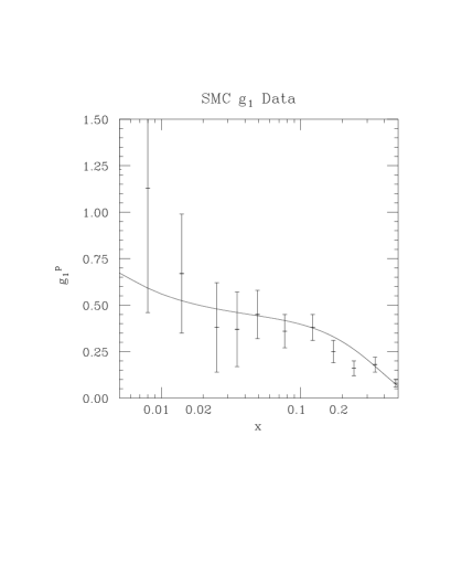
Figure 2: The $x$ dependent proton and neutron structure functions, $g_{1}^{p}$ and $g_{1}^{n}$ generated from Eqn. (71) and data. The dotted line represents the GRV-generated distributions and the solid line, MRS-generated distributions.

Figure 3: The $x$ dependent deuteron structure function, $g_{1}^{d}$, using the same technique as in figure 2.

3.3.3 Open Physics Questions

The proceeding analyses emphasize a number of key physics questions which the latest DIS experiments have raised. These include, but are not limited to:

• the size and sign of the polarized gluon distribution

• the amout of spin carried by the strange sea

• the light quark flavor dependence of polarization; is there an analogy to violation of Gottfried sum rule in $\Delta u$ and $\Delta d$?

• the connection, if any, between the unpolarized and the polarized distributions

• the role of the higher order corrections at low $x$ and $Q^{2}$-both perturbative and higher twist (non-perturbative)

• the role of the orbital motion, $L_{z}$; does it agree with the expected asymptotic values? [80]
  

Theoretical models which agree with present data still disagree on many of these points. It is therefore up to the experiments to decide which of these explain the various aspects of constituent spin contributions to the nucleons. In the next section, we outline the various polarization experiments which will address these issues.

3.4 Future Experiments

3.4.1 Introduction

There are a number of experiments which are technologically feasible that would supply some of the missing information about these distributions. Detailed summaries can be found in references by Ramsey [98] and Nurushev. [99] We have seen that the existing data have enabled us to formulate appropriate questions which probe the spin properties of nucleons. However, there are a number of questions which remain unanswered and will only be accessible with more data at different energies and momentum transfers. Fortunately, there are a number of experimental groups that are planning polarized beam experiments at existing accelerators. With recent advances in polarized beam, target, detector and accelerator technology, it is now possible to do these experiments at higher energies and momenta in order to study the physics over a large kinematic range. The large average luminosities of these experiments and the success of Siberian Snakes makes all of the following feasible. This section will include some of the proposed experiments related to the spin structure of nucleons, in light of the questions presented in the last section.

One of the ways to categorize polarization data is as follows:

• deep-inelastic scattering of polarized leptons (e, $\mu$) on polarized nucleon targets ($p$, $n$, $d$)

• photo-production of jets in high energy polarized $ep$ colliders

• production of pions and direct photons in polarized $pp$ and $p\bar{p}$ scattering

• charmed meson production (J/$\psi$ and $\chi$) in $pp$ collisions

• direct photon and jet production in polarized $pp$ collisions

• lepton pair production (Drell-Yan) in polarized processes

• heavy baryon (hyperon) production in unpolarized $pp$ collision

All of these are designed with the measurement of particular distributions in mind. Some can also provide crucial tests of QCD. There are a number of these presently planned at the following locations (alphabetically): (1) CERN (Switzerland), (2) DESY (Germany), (3) LISS (Indiana, USA), (4) RHIC (Brookhaven, USA), (5) Serpukhov (Russia) and (6) SLAC (USA). A partial list of experiments with their corresponding energies is given in Table V. This is to give a general idea of the wide range of energies and kinematic regions to be covered.

Table V

Experiment	Location	Energy $\sqrt{s}(GeV/c)$	Luminosity (cm-2 s-1)
HERMES	HERA (DESY)	$30\>(e)$ on $820\>(p)$	$2\cdot 10^{31}$
SPIN	HERA (DESY)	820	$2\cdot 10^{31}$
RHIC	Brookhaven	$60\to 500$	$2\cdot 10^{32}$
LISS	Indiana	20	$1\cdot 10^{32}$
COMPASS	CERN	120	$1\cdot 10^{32}$
NEPTUN-A	Serpukhov	400	$1\cdot 10^{31}$
E155	SLAC	48 (e)	—

In the following discussion, we will describe some of these experiments with regard to the physics that they probe, namely:

• a. $\Delta q$ measurements (valence and sea)

• b. $\Delta G$ measurement

• c. $L_{z}$ determination

• d. Nuclear measurements - $F_{2}^{D}$, $g_{1}^{A}$, $h_{1}^{N,D}$

• e. higher order corrections and other tests of QCD

A partial list of the experiments for these categories is in Table VI. These will be discussed in the following subsection. The experiments discussed here represent a sampling of those which directly relate to the subject of the spin structure of nucleons. Many of these are just a small fraction of the polarization experiments which can be performed at these accelerators, but they form an integral part of the program.

Table VI

Experiment	Proposed Type	Measured Quantities	Distribution
HERMES	DIS	$A_{1}^{p}$, $g_{1}^{p}$	$\Delta q$, $\Delta G$
E155	DIS	$g_{1}^{p}$, $g_{1}^{d}$	$\Delta q$, $\Delta g$
SPIN	Elastic pp	$A_{N}$, $A_{NN}$	Helicity NC
RHIC/COMPASS	Charm prod.	$A^{c}$	$\Delta G$
RHIC (STAR)	Jet, $\pi$, $\gamma$ prod	$\Delta\sigma_{L}$, $A_{LL}$	$\Delta G$
RHIC (PHENIX)	Drell-Yan	$A^{DY}$	$\Delta S$
LISS	Inelastic	$\sigma_{L}$, $\sigma_{T}$, $\Delta\sigma_{L}$	$\Delta G$
SLAC	Charm prod.	$A^{c}$	$\Delta G$
SLAC	W± prod	$A^{W}$	$\Delta q_{i}$
LHC	W± prod	$A^{W}$	$\Delta G$

3.4.2 Valence and Sea sensitive experiments

Deep Inelastic Scattering: The E155 experiment has been approved at SLAC. This experiment is designed to probe slightly smaller $x$ while greatly improving statistics and systematical errors. With lower error bars at small $x$, the extrapolation should achieve a more accurate value for the integrated distributions and narrow the ranges of constituent spin contributions even further.

There has been considerable discussion about performing the COMPASS polarization experiments at the LHC at CERN. Depending on the approved experiments, there is the possibility of probing small $x$ and doing polarized inclusive experiments to measure both sea and gluon contributions to proton spin. These could be made in complementary kinematic regions to those of the other accelerators. There are tentative plans to do polarized $W^{\pm}$ production, which provides a measure of the $x$-dependent sea distributions. Polarized $W^{\pm}$ production is also planned at SLAC and would provide useful flavor dependent sea information in a slightly different kinematic region than that of CERN.

The latest experiments at HERA in Hamburg have accelerated a large flux of polarized electrons from the storage ring and collided them with a gaseous target. The gaseous target has helped to eliminate some of the systematic errors characteristic of solid targets, which were used in the other experiments. This can be repeated for proton targets to test the BSR. With more events and the lower error bars at small $x$, it will be easier to extrapolate $g_{1}^{p}(x)$ and achieve a more accurate integrated value, $\langle g_{1}^{p}\rangle$. Thus, comparison to the Bjorken and Ellis-Jaffe sum rules will be more accurate, as will the ability to determine the polarized sea values from this data. [83, 100]

Anselmino, et. al., [101] have proposed doing charged current interactions ($l^{\pm}p\to\nu X$), which could measure various linear combinations of flavor dependent polarized distributions. These experiments are feasible and could put further constraints on the quark contributions to spin.

Tests of the valence quark polarized distributions can be made, provided a suitable polarized antiproton beam of sufficient intensity could be developed. [102] This would provide a good test of the Bjorken sum rule via measurement of $\langle\Delta q_{v}\rangle$ and the assumption of a flavor symmetric up and down sea.

Lepton pair production (Drell-Yan) processes provide another clean measure of the polarized sea. [103] The Relativistic Heavy Ion Collider (RHIC) at Brookhaven is designed to be an accelerator of both light and heavy ions. [104] The high energy community has proposed that polarized $pp$ and $p\bar{p}$ experiments be performed, due to the large energy and momentum transfer ranges which should be available. The energy range will be made in discrete steps between 50 and 500 GeV, and the momentum transfer range also covers a wide kinematic region. There are two main proposed detectors, STAR and PHENIX, which have different but complementing capabilities. Polarized Drell-Yan experiments are planned, which would give reasonable estimates to the polarized sea for each flavor. The PHENIX detector is suitable for lepton detection and the wide range of energies and momentum transfers could yield a wealth of Drell-Yan data over a wide kinematic range. The x-dependence of the polarized sea distributions could then be extracted to a fair degree of accuracy. Kamal [105] has calculated next-to-leading order (NLO) corrections to Drell-Yan processes and has made predictions for RHIC energies.

There has been a major effort to propose a double polarized $pp$ mode at HERA, which would accelerate polarized protons. There is a wealth of both inclusive and exclusive experiments that can be done there at an energy range complementary to that of the other accelerators. This would require a major upgrade and installation of Siberian snakes, but the physics output potential is great. This initiative would be labeled HERA-$\vec{N}$. For a comprehensive review of the prospects at HERA-$\vec{N}$, see the proceedings of the workshop at Zeuthen [106] and references by Anselmino, et. al., [107] and Nowak. [108] Gehrmann and Stirling [27] have calculated the NLO Drell-Yan asymmetries for both unpolarized and polarized experiments at HERA-$\vec{N}$ energies. Combining these with the RHIC measurements would give a good measure of the polarized sea over a large energy range.

3.4.3 Gluon sensitive experiments

Knowledge of the polarized gluon distribution is important for both the anomaly contribution to nucleon spin and to its over-all spin contribution via the $J_{z}$ sum rule discussed earlier. Thus, experiments sensitive to $\Delta G$ are a high proirity item. The following is a brief discussion of the possible gluon sensitive experiments and their corresponding proposed lacations.

(1) Jet production in polarized $ep$ collisions: It has been suggested that $\Delta G$ could be measured in $ep$ collisions which produce one or two jets of hadrons from the photon-gluon fusion process. [109, 110] This experiment could be done at HERA, but the experted asymmetries, even for a large polarized gluon distribution are only at the few percent level and may be difficult to measure with a sufficient degree of certainty to distiguish between the gluon models.

(2) Jet production in $pp$ collisions: Even before the spin crisis was popular, it was known that jet production in polarized $pp$ collisions could be a sensitive measure of $\Delta G$. [111] The STAR detector at RHIC is suitable for inclusive reactions involving jet measurements. This would provide an excellent measurement of the $Q^{2}$ dependence of $\Delta G$ due to the large range of energies available there. The NLO corrections to photon plus jet production have been calculated by Gordon. [112] The corresponding asymmetries range from a few percent for small gluon polarization to about 30% at HERA energies, if $\Delta G$ is large. Should DESY proceed with plans to polarize their proton beam, this experiment could be performed there, complementing the kinematic regions covered by RHIC and CERN.

(3) Direct photon and double photon production: A clean signature for $\Delta G$, but one that is harder to measure, is that of direct photon production, ($\vec{p}\vec{p}\to\gamma\>+\>X$). [29, 113] The NLO corrections have been calculated for HERA-$\vec{N}$ [114, 115] and RHIC. [116] Although the asymmetries are only very large for the largest gluon models, the signal is clean and could distinguish if $\Delta G$ is large. Numerical simulations have been done in NLO for the double photon production processes ($\vec{p}\vec{p}\to\gamma\gamma\>+\>X$). [117] At RHIC energies, the asymmetries can be from a few percent to 20% for the larger $\Delta G$, but the cross sections arequite small for the optimal momenta (picobarns or smaller). Thus, it is unclear whether this is viable unless very high luminosities can be reached.

(4) Charm production in polarized collisions are also sensitive to $\Delta G$ and should be performed at both RHIC and HERA-$\vec{N}$. The double spin assymetries for J/$\psi$ production have been calculated and are sensitive to the color-octet contribution. [118, 119] These asymmetries are only on the few to 10% level. The two-spin asymmetries for $\chi$ production have also been calculated. [120] These asymmetries are quite small unless the polarized gluon distribution is quite large ($\langle\Delta G\rangle\approx 6$). Thus, $\chi$ production could distinguish an extremely large distribution from other models. Open charm production from lepton-hadron scattering has been proposed at LHC by the COMPASS group. [8, 121, 122] This provides another method to measure the photon-gluon fusion process and has very small uncertainties associated with the proposed experiment. These asymmetries can be quite large and provide a good potential for extending our knowledge of $\Delta G$.

(5) Inclusive reactions involving pion production would be alternate tests of the $Q^{2}$ dependence of $\Delta G$. [102] These could be done at any of the aforementioned accelerators and would provide a good cross check of measurements of $\Delta G$ in similar kinematic regions.

3.4.4 Experiments Probing Higher order QCD Effects

There are other polarized experiments which would provide tests of QCD and give a measure of some of the higher twist effects which were previously discussed.

(1) Elastic scattering, especially at a large $-t$ range, could shed light on both helicity non-conservation at the hadronic level and non-perturbative long range effects. Elastic experiments have been proposed for HERA, RAMPEX at Serpukhov and LISS in Indiana. [123]

(2) Recently, a proposal for a new light ion accelerator was announced, which will specialize in polarization experiments. [124] The Light Ion Spin Synchrotron (LISS) would be located in Indiana to perform a variety of polarization experiments for both high energy and nuclear physics. The energy range would be lower that most other experiments, thus complementing the kinematic areas covered. Furthermore, both proton and deuteron beams could be available to perform inclusive scattering experiments. They propose to measure longitudinal and transverse cross sections and spin asymmetries, which will address the normalization of the proton wave function. Elastic scattering measurements of $A_{N}$ at moderate momentum transfer $-t$ could give valuable information regarding helicity non-conservation in this region.

(3) Measurement of the transverse spin and transversity distributions would probe higher-twist non-perturbative effects as well. [125] The higher twist parton distributions could also be measured at RHIC and HERA. [126, 127, 128]

(4) Single spin asymmetries in DIS (where only one of the scatterers is polarized) have been calculated by many groups. These provide helicity conservation tests as well as measures of higher twist processes. [129, 79, 78] These experiments could be done at HERA. The $pp$ single spin asymmetries can also be done at HERA, RHIC and the LHC. These are good measurments of higher twist contributions to the structure functions. The $pp$ single spin experiments are also planned by the RAMPEX collaboration (Russian-AMerican Polarization EXperiment). [130]

This is a summary of some of the key experiments which will answer the questions posed throughout this review. There are many other important polarization experiments which test QCD and non-standard physics, but they will not be covered here. However, from this list alone, it is easily seen that polarization experiments are crucial to our understanding of the most fundamental properties of the elementary particles.

3.5 Conclusion

This review has outlined the key theoretical and experimental elements which have contributed to our understanding of the constituents’ contribution to the spin of nucleons. Analyses of existing data indicate that the spin structure of nucleons is non-trivial and has led to the formulation of a crucial set of questions to be answered about this structure. The key remaining questions are related to the strange sea and gluon polarizations. The experiments discussed here can be performed in order to shed light on these questions. In performing these experiments, an added benefit is that crucial tests of QCD and the quark model will be simultaneously be made. The questions of factorization and validity of the sum rules are among the questions which can be addressed. In the past few years, theorists have made considerable progress in calculating higher order corrections to the appropriate sum rules and structure functions and experimentalists have added more accurate and comprehensive DIS data. This has contributed to narrowing the range of possible spin contributions from the constituents, but has also raised other questions about spin structure of nucleons.

There is still much work to be done in constructing a suitable model for spin transfer among constituents, along with calculating higher order corrections to the various spin processes which can be used to test the models. There are many experiments planned at various locations, which will create work for the experimentalists and phenomenologists. These suggestions do not include some of the other areas of probing spin phenomena, mentioned at the beginning of this review. These other areas cover the spectrum of both high energy and medium energy nuclear physics as well. Thus, we are in an interesting period of spin physics. One where considerable progress has been made, only to discover that there is much more to be done to increase our understanding of the fundamental nature of matter through the use of polarization.

References

Other Review papers with related but complementary information:

M. Anselmino, et. al., Phys. Rep. 261, 1, (1995)
D. Bass and A. W. Thomas, Prog. Part. Nucl. Phys., 33, (1994)
H.-Y. Cheng, Int. J. Mod. Phys., A11, 5109, (1996) (also hep-ph/9607254)
J. Ellis and M. Karliner, hep-ph/9601280 (CERN-TH/95-334; TAUP-2316-96)
B. Frois, Prog. Part. Nucl. Phys., 34, (1995)
I. Hinchcliffe and A. Kwiatkowski, hep-ph/9604210 (LBL-38549)
S.E. Troshin and N.E. Tyurin, Particle World 3, 165, (1993).

References cited in paper:

References

- [1] M. J. Alguard, et. al., Phys. Rev. Lett. 37, 1258, (1976); ibid., 37, 1261, (1978); ibid., 41, 187, (1978); G. Baum, et. al., Phys. Rev. Lett. 51, 1135, (1983)
- [2] J. Ashman, et. al., Phys. Lett. B206, 364, (1988) and Nucl. Phys. B328, 1, (1989)
- [3] J. D. Bjorken, Phys. Rev. 148, 1467, (1966)
- [4] J. Ellis and R.L. Jaffe, Phys. Rev. D9, 1444, (1974), erratum Phys. Rev. D10, 1669, (1974).
- [5] F. E. Close and R. G. Roberts, Phys. Rev. Lett. 60, 1471, (1988); S. J. Brodsky, J. Ellis and M. Karliner, Phys. Lett. B206, 309, (1988); M. Anselmino, B. L. Ioffe, and E. Leader Yad. Fiz., 49, 214, (1989); H. Lipkin, Phys. Lett. B256, 284, (1991); J.-W. Qiu, et. al., Phys. Rev. D41, 65, (1990)
- [6] B. Adeva, et. al., Phys. Lett. B320, 400, (1994); D. Adams, et. al., Phys. Lett. B329, 399, (1994), Phys. Lett. B336, 125, (1994) and Phys. Lett. B357, 248, (1995)
- [7] P. L. Anthony, et. al., Phys. Rev. Lett. 71, 959, (1993)
- [8] Talks by G. K. Mallot and A. Simon, to be published in the proceedings of the 12th International Symposium on High Energy Spin Physics (Spin’96), Amstersdam, The Netherlands, September, 1996. See also hep-ex/11016.
- [9] M. Goshtasbpour and G. P. Ramsey, hep-ph/9512250 and hep-ph/9611216
- [10] D. L. Adams, et. al., (FNAL E581/704 Collaboration), Phys. Lett. B336, 269, (1994) and D. P. Grosnick, ANL-HEP-PR-96-36.
- [11] J. D. Bjorken, Phys. Rev. 179, 1547, (1969)
- [12] R. G. Roberts, The Structure of the Proton, c1990, Cambridge University Press.
- [13] M. Anselmino, et. al., hep-ph/9607334
- [14] P. J. Mulders, and R.D. Tangerman, Nucl. Phys. B461, 197, (1996) and P. J. Mulders, nucl-th/9611040
- [15] S. Wandzura and F. Wilczek, Phys. Lett. 72B, 195, (1977)
- [16] H. Burkhardt and W. N. Cottingham, Ann. Phys. 56, 453, (1970)
- [17] K. Abe, et. al., Phys. Rev. Lett. 74, 346, (1995) and Phys. Rev. Lett. 75, 25, (1995) and hep-ex/9610007
- [18] J. Kodaira, Y. Yasui, K. Tanaka and T. Uematsu, Phys. Lett. B387, 855, (1996); R. G. Roberts and D. Bass, hep-ph/9601235; W.-M. Zhang and A. Harindranath, hep-ph/9606347
- [19] A. Kotikov and D.V. Peshekhonov, Phys. Rev. D54, 3162, (1996)
- [20] M. Glück, E. Reya and W. Vogelsang, Phys. Lett. B359, 201, (1995)
- [21] E. Stein, et. al., Phys. Lett. B353, 107, (1995)
- [22] M. Meyer-Hermann, et. al., Phys. Lett. B383, 463, (1996)
- [23] D. Boer and R. D. Tangerman, hep-ph/9603428
- [24] G. R. Farrar and D. R. Jackson, Phys. Rev. Lett. 35, 1416, (1975)
- [25] F. E. Close and D. Sivers, Phys. Rev. Lett. 39, 1116, (1977)
- [26] J. Bartelski and S. Tatur, Z. Phys. C71, 595, (1996)
- [27] T. Gehrmann and W.J. Stirling, Phys. Rev. D53, 6100, (1996)
- [28] P. Chiapetta and J. Soffer, Phys. Rev. D31, 1019 (1985)
- [29] J.-W. Qiu, G. P. Ramsey, D. G. Richards and D. Sivers, Phys. Rev. D41, 65, (1990)
- [30] G. Altarelli and G. Parisi, Nucl. Phys. B126, 298, (1977) and V. N. Gribov and L. N. Lipatov, Yad. Fiz. 15, 781, (1972) and Sov. J. Nucl. Phys. 15, 438, (1972)
- [31] W. Furmanski and R. Petronzio, Nucl. Phys. B195, 237, (1982)
- [32] J. Blümlein, et. al., hep-ph/9609400 (DESY 96-199)
- [33] A. D. Martin, R.G. Roberts and W.J. Stirling, Phys. Rev. D50, 6734, (1994), Phys. Lett. B354, 155, (1995) and Phys. Lett. B387, 419, (1996)
- [34] M. Glück, E. Reya and A. Vogt, Phys. Lett. B306, 391, (1993) and Phys. Rev. D53 4775, (1996); A. Vogt, Phys. Lett. B354, 145, (1995)
- [35] H. L. Lai, hep-ph/9606399
- [36] M. Derrick, et. al., Z. Phys. C65, 379, (1995) and T. Ahmed, et. al., Phys. Lett. B348, 681, (1995)
- [37] J. Botts, et. al., Phys. Lett. B304, 159, (1993); H. L. Lai, et. al., Phys. Rev. D51, 4763, (1995) and hep-ph/9606399; W.-K. Tung, hep-ph/9608293
- [38] P. Armaudruz, et. al., Phys. Rev. Lett. 66, 2712, (1991)
- [39] K. Gottfried, Phys. Rev. Lett. 18, 1174, (1967)
- [40] A. Baldit, et. al., Phys. Lett. B332, 244, (1994)
- [41] B. R. Webber, hep-ph/9607404
- [42] C. Lopez, F. Barreiro and F.J. Yndurain, hep-ph/9605395
- [43] J. Collins, hep-ph/9610330
- [44] H.-Y. Cheng, hep-ph9512267 (IP-ASTP-25-95)
- [45] H.-Y. Cheng, Int. J. Mod. Phys. A11, 5109, (1996)
- [46] G. T. Bodwin and J.-W. Qiu, Phys. Rev. D41, 2755, (1990)
- [47] R. Carlitz, J. C. Collins and A. H. Mueller, Phys. Lett. B214, 229, (1988)
- [48] M. Goshtasbpour and G. P. Ramsey, proceedings of the VI workshop on High Energy Spin Physics, Protvino, c1996 and proceedings of the 12th International Symposium on High Energy Spin Physics (Spin’96), Amstersdam, The Netherlands, September, 1996; G. P. Ramsey, hep-ph/9611246
- [49] W. Celmester and D. Sivers, Ann. Phys. 143, 1, (1982)
- [50] I. Hinchcliffe and A. Kwiatkowski, hep-ph/9604210 (LBL-38549); B. L. Ioffe, hep-ph/9511264
- [51] J. Ellis and M. Karliner, CERN-TH/95-334 (hep-ph/9601280)
- [52] F. E. Close and R.G. Roberts, Phys. Lett. B316, 165, (1993)
- [53] S. A. Larin, F. V. Tkachev and J. A. M. Vermaseren, Phys. Rev. Lett. 66, 862, (1991) and S.A. Larin and J.A.M. Vermaseren, Phys. Lett. B259, 345, (1991); S.A. Larin, Phys. Lett. B334 192, (1994)
- [54] J. Ellis, et. al., Phys. Lett. B366, 268, (1996)
- [55] H. J. Lipkin, Phys. Lett. B337, 157, (1994)
- [56] S. Okubo, Phys. Lett. 5, 165, (1963); G. Zweig, CERN Report 8419/TH412 (1964, unpublished); I. Iuzuka, Prog. Theor. Phys. Suppl. 37-38, 21, (1966)
- [57] X. Ji, hep-ph/9610369
- [58] G. Preparata, P.G. Ratcliffe and J. Soffer, Phys. Lett. B273, 306, (1991) and Phys. Rev. D42, 930, (1990); G. Preparata and J. Soffer, Phys. Rev. Lett. 61, 1167, (1988) and Phys. Rev. Lett. 62, 1213, (1989)
- [59] B. L. Ioffe and M. Karliner, Phys. Lett. B247, 387, (1990)
- [60] T. Gehrmann and W.J. Stirling, hep-ph/9608468
- [61] B.-Q. Ma, Proc. of the Second International Symposium on Medium Energy Physics, Beijing, China, Aug. 22-26, 1994, Eds. W. Chao and P. Shen, World Scientific, Singapore, 1995 and hep-ph/9604422.
- [62] A. E. Dorokhov and N.I. Kochelev, Phys. Lett. B304, 167, (1993)
- [63] G. Cates, to be published in the proceedings of the 12th International Symposium on High Energy Spin Physics (Spin’96), Amstersdam, The Netherlands, September, 1996.
- [64] A. V. Efremov, O.V. Teraev and E. Leader, hep-ph/9607217
- [65] R. Hamberg and W.L. van Neerven, Nucl. Phys. B379, 143, (1992); E. B. Zijlstra and W.L. van Neerven Nucl. Phys. B417, 61, (1994) and B426, 245, (1994); R. Mertig and W.L. van Neerven, Z. Phys. C70, 637, (1996); W. Vogelsang, Phys. Rev. D54, 2023, (1996)
- [66] J. Blümlein and A. Vogt, hep-ph/9610203 and Phys. Lett. B386, 350, (1996); J. Blümlein S. Riemersma and A. Vogt, hep-ph/9608470 (DESY 96-131)
- [67] T. Weigl and W. Melnitchouk, Nucl. Phys. B465, 267, (1996)
- [68] X. Ji and C. Chou, Phys. Rev. D42, 3637, (1990)
- [69] R. Carlitz and J. Kaur, Phys. Rev. Lett. 38, 673, (1977)
- [70] S.-J. Dong, J.-F. Lagaë and K. F. Liu, Phys. Rev. Lett. 75, 2096, (1995)
- [71] B.-A. Li, et. al., Phys. Rev. D43, 1515, (1991)
- [72] G. P. Ramsey, et. al., Phys. Rev. D39, 361, (1989)
- [73] R. L. Jaffe, Phys. Rev. D54, 6581, (1996)
- [74] N. Kochelev, hep-ph/9610551
- [75] E. Di Salvo, hep-ph/9603286
- [76] W.-D. Nowak, et. al., hep-ph/9608463
- [77] G. Altarelli and G. G. Ross, Phys. Lett. B212, 391, (1988); R. Carlitz, J. C. Collins and A. H. Mueller, Phys. Lett. B214, 229, (1988); A. V. Efremov and O. V. Teryaev, JINR Report E2-88-287 (unpublished); R. L. Jaffe, Phys. Lett. B193, 101, (1987)
- [78] C. Boros, Z. Liang, T. Meng and R. Rittel, Phys. Rev. Lett. 70, 1751, (1993); C. Boros, Z. Liang, T. Meng and R. Rittel, hep-ph/9610487
- [79] S. M. Troshin and N.E. Tyurin, hep-ph/9610241
- [80] X. Ji, et. al., Phys. Rev. Lett. 76, 240, (1996)
- [81] A. V. Radyushkin, Phys. Lett. B380, 417, (1996)
- [82] J. Ellis and M. Karliner Phys. Lett. B341, 397, (1995)
- [83] R. D. Ball, S. Forte and G. Ridolfi, Phys. Lett. B378, 255, (1996)
- [84] Y. Y. Balitskiĭ and L.N. Lipatov, Sov. J. Nucl. Phys. 28, 822, (1978); E. A. Kureav, et. al., JETP 45, 199, (1977); L. N. Lipatov, JETP 63, 904, (1986)
- [85] J. Bartels, B. I. Ermolaev and M. G. Ryskin, Z. Phys. C70, 273, (1996)
- [86] P. Ratcliffe, hep-ph/9611348
- [87] J. Soffer and O.V. Teraev, hep-ph/9609329
- [88] W. Buchmüller and D. Haidt, hep-ph/9605428 (DESY 96-061)
- [89] M. Glück, E. Reya, M. Stratmann and W. Vogelsang, Phys. Rev. D53, 4775, (1996)
- [90] T. P. Cheng and L.-F. Li, Phys. Rev. Lett. 74, 2872, (1995)
- [91] B. Frois, Prog. Part. Nucl. Phys., 34, (1995)
- [92] D. G. Crabb and D. B. Day, Nucl. Instr. and Meth. in Phys. Res. 356A, 9, (1995)
- [93] J. Szwed, hep-ph/9605294
- [94] See also papers in AIP Conf. Proc. 343, 75, (1995). Proceedings of the 11th International Symposium on High Energy Spin Physics, (Indiana, Sep, 1994), c1995, on the following topics: Polarized Beams-Snakes (Huang), Sources (L.W. Anderson), Polarized Targets (W. Meyer)
- [95] See also papers in the Proceedings of the 12th International Symposium on High Energy Spin Physics, (Amsterdam, Sep, 1996), on the following topics: Polarized Beams-Snakes (Anferov), Polarized Targets-Solid (St. Goertz, B. Owen), Gaseous (V.G. Luppov); Detectors–Polarimeters: A. Feltham, P. Schuler, G. Igo, D. Underwood, E. Burtin
- [96] S. Platchkov, preprint DAPNIA SPhN 93-53: invited talk at the 14th Eur. Conf. on Few Body Problems, Amsterdam, 1993
- [97] S. Alekhin, hep-ph/9611213 (IHEP 96-79)
- [98] G. P. Ramsey, Particle World, 4, 11, (1995)
- [99] S. B. Nurushev, IHEP preprint IHEP 91-103, Protvino, Russia.
- [100] C. Bourrely, et. al., hep-ph/9604204 and hep-ph/9609515
- [101] M. Anselmino, P. Gambino and J. Kalinowski, hep-ph/9607427
- [102] G. P. Ramsey and D. Sivers, Phys. Rev. D43, 2861, (1991)
- [103] H.-Y. Cheng and S.-N. Lai, Phys. Rev. D41, 91, (1990)
- [104] RHIC Spin Collaboration, ”Proposal on Spin Physics Using the RHIC Polarized Collider”, August, 1992; and STAR-RSC Update, October, 1993.
- [105] B. Kamal, Phys. Rev. D53, 1142, (1996)
- [106] J. Blümlein and W.-D. Nowak, Eds., Workshop on the Prospects of Spin Physics at HERA, Zeuthen, August 28-31, 1995.
- [107] M. Anselmino, et. al., hep-ph/9608393
- [108] W.-D. Nowak, hep-ph/9605411 (DESY 96-095)
- [109] M. Stratmann, and W. Vogelsang, hep-ph/9605330 (DO-TH 96/10)
- [110] A. DeRoeck, et. al., hep-ph/9610315 (DESY 96-197)
- [111] G. P. Ramsey, G. P., D. Richards and D. Sivers, Phys. Rev. D37, 3140, (1988)
- [112] L. E. Gordon, hep-ph/9609403 (ANL-HEP-PR 96-78) and ANL-HEP-PR-96-59
- [113] E. L. Berger and J.-W. Qiu, Phys. Rev. D40, 778, (1989)
- [114] A. P. Contogouris and Z. Merebashvili, hep-ph/9611401
- [115] L. E. Gordon and W. Vogelsang, Phys. Lett. B387, 629, (1996)
- [116] L. E. Gordon, ANL-HEP-PR-96-100
- [117] C. Coriano and L. Gordon, Phys. Rev. D49, 170, (1994) and Phys. Rev. D54, 781, (1996)
- [118] T. Gehrmann, Phys. Rev. D53, 5310, (1996)
- [119] O. Teraev and A. Tkabladze, hep-ph/9612301
- [120] T. Morii, S. Tanaka and T. Yamanishi, Phys. Lett. B372, 165, (1996)
- [121] B. Lampe, hep-ph/9608400
- [122] N. Horikawa, to be published in the proceedings of the Circum-Pan-Pacific Workshop on High Energy Spin Physics, Kobe, Japan, October, 1996.
- [123] G. P. Ramsey and D. Sivers, Phys. Rev. D47, 93, (1993)
- [124] J. M. Cameron and S. Vigdor, ”The LISS Brief”, proceedings of the XI International Symposium on High Energy Spin Physics, Bloomington, IN, September, 1994; c 1995, AIP.
- [125] R. L. Jaffe and N. Saito, hep-ph/9604220
- [126] Kirschner, et. al., hep-ph/9606267
- [127] G. Ladinsky, hep-ph/9601287
- [128] F. C. Khanna and A. Y. Umnikov, hep-ph/9609356
- [129] M. Anselmino, et. al., hep-ph/9610407
- [130] Yu. Arestov, to be published in the proceedings of the 12th International Symposium on High Energy Spin Physics, Amsterdam, September, 1996.