Radiative Corrections to the Muonium Hyperfine Structure.
II. The $\alpha(Z\alpha)^{2}$ Correction

Abstract

This is the second of a series of papers on the radiative corrections of order $\alpha^{2}(Z\alpha)$, $\alpha(Z\alpha)^{2}$, and various logarithmic terms of order $\alpha^{4}$, to the hyperfine structure of the muonium ground state. This paper deals with the $\alpha(Z\alpha)^{2}$ correction. Based on the NRQED bound state theory, we isolated the term of order $\alpha(Z\alpha)^{2}$ exactly. Our result $+16.904~{}2~{}(11)\alpha(Z\alpha)^{2}E_{F}/\pi$ for the non-logarithmic part is consistent with the $\alpha(Z\alpha)^{2}$ part of Sapirstein’s calculation and the recent result of Pachucki, and reduces the numerical uncertainty in the $\alpha(Z\alpha)^{2}$ term by two orders of magnitude.

I Introduction

Now that the $\alpha^{2}(Z\alpha)$ correction to the hyperfine splitting of the ground state muonium is known very accurately because of recent works [1, 2, 3], the previously-calculated $\alpha(Z\alpha)^{2}$ term has become one of the main sources of the remaining theoretical uncertainty. Improvement of this error is urgently needed in view of the new muonium hyperfine measurement in progress [4]. Here $Z$ is the $``$atomic” number of the nucleon. Of course $Z=1$ for the muonium, but it is kept to indicate the bound state origin of the correction terms. In this paper, we present the $\alpha(Z\alpha)^{2}$ radiative correction evaluated in the NRQED bound state formulation [5].

The previous evaluation of this term, including recent modifications [3, 6], gives

$$\Delta\nu[\alpha(Z\alpha)^{2}] = E_{F}{\alpha(Z\alpha)^{2}\over\pi}\biggl{[}-{8\over 3}\ln^{2}(Z\alpha)^{-1}$$ (2)

$$+\left(-{8\over 3}\ln 4+{37\over 36}+{8\over 15}\right)\ln(Z\alpha)^{-1}+14.88~{}(29)~{}\biggr{]}~{}~{}~{},$$

where the Fermi frequency $E_{F}$ is defined by [7]

$$E_{F}={16\over 3}\alpha^{2}cR_{\infty}{{m}\over{M}}\left[1+{m\over M}\right]^{-3},$$ (3)

$R_{\infty}$ is the Rydberg constant for infinite nuclear mass, and $m$ and $M$ are the electron and muon masses, respectively. The presence of $\ln(Z\alpha)$ factors is due to the near infrared (IR) structure of the loosely bound state. The coefficients of $\ln^{2}(Z\alpha)^{-1}$ and $\ln(Z\alpha)^{-1}$ terms were obtained by Layzer [8] and Zwanziger [9] independently. Brodsky and Erickson [10] confirmed these logarithmic terms and gave the leading contribution of the non-logarithmic term. Sapirstein reported the numerical evaluation of the non-logarithmic constant due to the radiative photon [11]. For convenience’s sake, we refer to this non-logarithmic constant of the $\alpha(Z\alpha)^{2}$ correction as the BES term.

To compute the BES term, Sapirstein started from the relativistic bound state formalism and evaluated the entire $\alpha(Z\alpha)^{2}$ term numerically. In his approach, only the double logarithmic term was confirmed by varying the $``$atomic” number $Z$. Since the logarithmic term is a consequence of the near IR singularity of the bound state, the convergence of numerical integration worsens in the region of small momentum. The uncertainty in the BES term comes mainly from this difficulty in the numerical integration. Note also that his result contains terms of higher orders in $Z\alpha$.

Our calculation of the BES term starts from the NRQED formalism proposed by Caswell and Lepage [5]. This approach enables us to isolate the $\alpha(Z\alpha)^{2}$ term without being tangled up with higher order terms in $Z\alpha$: All these terms arise from different parts of the NRQED Hamiltonian. The leading logarithmic contribution is analytically separated. The small photon mass $\lambda$ is used in our approach but the $\lambda$ dependence can be easily identified and analytically subtracted in the numerical evaluation of each diagram. This is important for reducing the computational error of the BES term.

Asides from the factor $(\alpha(Z\alpha)^{2}/\pi)E_{F}$ our results for the vacuum polarization contribution and the radiative photon contribution to the BES term are

$$\Delta E_{\rm BESvp}=-0.218~{}567~{}\cdots~{},$$ (4)

and

$$\Delta E_{\rm BESph}=17.122~{}7~{}(11)~{},$$ (5)

respectively. Our final result for the total $\alpha(Z\alpha)^{2}$ correction is

$$\Delta\nu[\alpha(Z\alpha)^{2}] = E_{F}{\alpha(Z\alpha)^{2}\over\pi}\biggl{[}-{8\over 3}\ln^{2}(Z\alpha)^{-1}$$ (7)

$$+\left(-{8\over 3}\ln 4+{37\over 36}+{8\over 15}\right)\ln(Z\alpha)^{-1}+16.904~{}2~{}(11)~{}\biggr{]}~{}~{}~{}.$$

The BES term has also been evaluated recently by Pachucki [13] using the method he developed for the $\alpha(Z\alpha)^{6}m$ Lamb shift correction [14]. His result for the radiative photon contribution is

$$\Delta E_{\rm BESph}=17.122~{}.$$ (8)

Although this is in good agreement with our result (5), there remains some disagreement in the details. This will be discussed in Sec. VI.

In Sec. II, we briefly describe our approach, namely the NRQED method, to the bound state problem. A more detailed prescription of NRQED is found in Ref. [3]. In Sec. III, the well-known Breit $(Z\alpha)^{2}$ correction [15] is rederived from NRQED. This calculation, multiplied by an appropriate $``$renormalization” factor, actually provides a part of the $\alpha(Z\alpha)^{2}$ term. It also serves as a prototype of the calculation of the entire $\alpha(Z\alpha)^{2}$ correction. In Sec. IV we derive the $\alpha(Z\alpha)^{2}$ contribution arising ¿from the vacuum polarization insertion. We uncovered a mistake in the previous calculation in Ref. [10] as was mentioned in our previous paper [3]. The detail of the $\alpha(Z\alpha)^{2}$ correction due to the radiative photon on the electron line is described in Sec. V. Sec. VI is devoted to the discussion of our result.

II Outline of the NRQED method

The NRQED is a theory with a finite UV cut-off, which is completely equivalent to QED when it is applied to low-energy systems with typical momenta less than the UV cut-off $\Lambda$. The NRQED Lagrangian consists of operators which satisfy the same symmetries as the QED operators except that they satisfy Galileian invariance, although the final observable results of calculation are Lorentz invariant. Fermions are represented not by Dirac spinors but by Pauli spinors. The NRQED Lagrangian can be divided into two parts: The main part $L_{\rm main}$ consisting of fermion bilinear operators multiplied by up to two photon operators or pure photon terms and the contact interaction part $L_{\rm contact}$ involving four or more fermions. Both parts of the Lagrangian are determined by the following simple rule: The operators which appear in its Lagrangian and their coefficients are chosen so that any $scattering$ amplitude calculated in the NRQED coincides with the corresponding $scattering$ amplitude of the original QED at some given momentum scale, e.g., at the threshold of the external on-shell particles. This matching condition is applied order by order to the expansion in the coupling constant $\alpha$ and velocity $v$ of the external fermion. The Coulomb gauge is used in the NRQED, while the Feynman gauge is more convenient to compute the QED scattering diagrams. Readers interested in NRQED may refer to Refs. [5, 16, 17, 18, 19]. The precise description of the NRQED Hamiltonian can be found in Ref.[3]. After determining all operators and their coefficients to the desired order of velocity $v$ of the electron and the coupling constant $\alpha$, we evaluate the energy shift, etc. using the Rayleigh-Schrödinger perturbation theory, choosing as the unperturbed system the exact solution of the nonrelativistic Schrödinger Coulomb system.

The main part of the NRQED Hamiltonian $H_{\rm main}^{\Lambda}$ needed to compute the $\alpha(Z\alpha)^{2}$ correction terms is of the form

$$H_{\rm main}^{\Lambda}=\psi^{\dagger}(\vec{p}\,^{\prime})\biggl{[} {{\vec{p}\,^{2}}\over 2m}+eA^{0}-{(\vec{p}\,^{2})^{2}\over 8m^{3}}-{e\over 2m}(\vec{p}\,^{\prime}+\vec{p})\cdot\vec{A}$$ (9)

$$- {ie\over 2m}c_{F}\vec{\sigma}\cdot(\vec{q}\times\vec{A})-{e\over 8m^{2}}c_{D}\vec{q}\,^{2}A^{0}$$ (10)

$$- {ie^{2}\over 4m^{2}}c_{S}\vec{\sigma}\cdot(\vec{q_{2}}\times\vec{A}(q_{1}))A^{0}(q_{2})+(q_{1}\leftrightarrow q_{2})$$ (11)

$$+ {ie\over 8m^{3}}c_{W}(\vec{p}\,^{\prime 2}+\vec{p}\,^{2})\vec{\sigma}\cdot(\vec{q}\times\vec{A})+{ie\over 8m^{3}}c_{q^{2}}\vec{q}\,^{2}\vec{\sigma}\cdot(\vec{q}\times\vec{A})$$ (12)

$$+ {ie\over 8m^{3}}c_{p^{\prime}p}\{\vec{p}\cdot(\vec{q}\times\vec{A})(\vec{\sigma}\cdot\vec{p}\,^{\prime})+\vec{p}\,^{\prime}\cdot(\vec{q}\times\vec{A})(\vec{\sigma}\cdot\vec{p})\}~{}~{}~{}\biggr{]}\psi(\vec{p})$$ (13)

$$+ c_{\rm vp}A^{i}(\vec{q}){\vec{q}\,^{4}\over m^{2}}A^{j}(\vec{q})(\delta^{ij}-{q^{i}q^{j}\over\vec{q}\,^{2}})$$ (14)

$$+ c_{\rm vp}A^{0}(\vec{q}){-\vec{q}\,^{4}\over m^{2}}A^{0}(\vec{q})~{},$$ (15)

where $\vec{p}$ and $\vec{p}\,^{\prime}$ are incoming and outgoing electron momenta, respectively, and $\vec{q}$ is incoming photon momentum. The superscript $\Lambda$ in $H_{\rm main}^{\Lambda}$ indicates that the theory is regularized by the UV cut-off $\Lambda$ for the radiative photon. $\Lambda$ may be less than $m$. The $``$renormalization” coefficients in (15) are

$$c_{F} = 1+a_{e}~{},$$ (16)

$$c_{D} = 1+{\alpha\over\pi}{8\over 3}\biggl{[}\ln\left({m\over 2\Lambda}\right)-{3\over 8}+{5\over 6}\biggr{]}+2a_{e}~{},$$ (17)

$$c_{S} = 1+2a_{e}~{},$$ (18)

$$c_{W} = 1~{},$$ (19)

$$c_{q^{2}} = {\alpha\over\pi}{4\over 3}\biggl{[}\ln\left({m\over 2\Lambda}\right)-{3\over 8}+{5\over 6}+{1\over 4}\biggr{]}+{a_{e}\over 2}~{},$$ (20)

$$c_{p^{\prime}p} = a_{e}~{},$$ (21)

$$c_{\rm vp} = {\alpha\over 15\pi}~{}.$$ (22)

The first term in (15) is the nonrelativistic kinetic energy term. The rest are named successively as Coulomb, $p^{4}$ relativistic kinetic energy, dipole coupling, Fermi, Darwin , seagull, $W$-(wave function) derivative Fermi, $q^{2}$ derivative Fermi, and $p^{\prime}p$ coupling, respectively. The last two terms bilinear in photon operators are introduced to represent the vacuum polarization insertion in the transverse and Coulomb photon propagator, respectively.

For the muon line, only the Coulomb and Fermi terms are needed for the calculation of the $\alpha(Z\alpha)^{2}$ correction. They are obtained by replacing $e$ and $m$ of the electron interaction terms by $-Ze$ and $M$, respectively .

As for the contact part of the NRQED Hamiltonian $H_{\rm contact}^{\Lambda}$, only the spin-flip type is needed:

$$H_{\rm contact}^{\Lambda}=-d_{1}{1\over mM}(\psi^{\dagger}\vec{\sigma}\psi)\cdot(\chi^{\dagger}\vec{\sigma}\chi),$$ (23)

where $\chi$ is the Pauli spinor for the positive muon and $d_{1}$ can be written as

$$-d_{1} = \alpha(Z\alpha)^{2}\pi{2\over 3}\biggl{[}\ln 2-{13\over 4}+{3\over 4}\biggr{]}$$ (24)

$$+ \alpha(Z\alpha)^{3}{2\over 3}\biggr{[}d^{(3)}\sqrt{{\Lambda m\over((Z\alpha)m)^{2}}}+d^{(2)}\ln^{2}\biggl{(}{\Lambda\over m}\biggr{)}+d^{(1)}\ln\biggl{(}{\Lambda\over m}\biggr{)}+d^{(0)}$$ (25)

$$+ d^{(4)}{\Lambda^{\prime}\over(Z\alpha)m}+d^{(5)}\ln\left({\Lambda^{\prime}\over m}\right)\biggr{]}.$$ (26)

Here $\Lambda^{\prime}$ is the UV cutoff of the transverse exchanged photon momentum. Note that, when the $\alpha(Z\alpha)^{2}$ part of Eq. (26) is evaluated in the first order perturbation theory, it gives the $\alpha(Z\alpha)$ correction to the hyperfine splitting of the ground state muonium calculated by Kroll and Pollock, and Karplus, Klein, and J. Schwinger [20]. For brevity, let us call the $\alpha(Z\alpha)$ correction as the KP correction. The coefficients $d^{(0)},\cdots,d^{(5)}$ of the $\alpha(Z\alpha)^{3}$ part of Eq. (26) are pure numbers. These are the quantities that we want to calculate in this paper.

The Green function $\tilde{G}_{0}(\vec{p},\vec{q};E)$ appearing in this calculation is known in an exact closed form for the nonrelativistic Coulomb potential [21]. For an arbitrary energy $E$ in the complex $E$ plane this function takes the form:

$$\tilde{G}_{0}(\vec{p},\vec{q};E) = -{2m\over\vec{p}\,^{2}+p_{0}^{2}}(2\pi)^{3}\delta^{3}(\vec{p}-\vec{q})$$ (29)

$$+{-2m\over\vec{p}\,^{2}+p_{0}^{2}}{-4\pi Z\alpha\over|\vec{p}-\vec{q}|^{2}}{-2m\over\vec{q}\,^{2}+p_{0}^{2}}$$

$$-{64\pi\over\gamma^{4}(Z\alpha)}\tilde{R}(\vec{p},\vec{q};E)~{}~{},$$

where

$$p_{0}^{2}=-2mE,~{}~{}~{}~{}~{}~{}\nu={\gamma\over p_{0}}~{},$$ (30)

and

$$\tilde{R}(\vec{p},\vec{q};E) = {\gamma^{7}p_{0}\over(\vec{p}\,^{2}+p_{0}^{2})(\vec{q}\,^{2}+p_{0}^{2})}$$ (32)

$$\times\int_{0}^{1}d\rho{\rho^{-\nu}\over 4\rho|\vec{p}-\vec{q}|^{2}p_{0}^{2}+(1-\rho)^{2}(\vec{p}\,^{2}+p_{0}^{2})(\vec{q}\,^{2}+p_{0}^{2})}~{}~{}.$$

The first, second, and third terms of (29) correspond to zero, one, and two or more Coulomb-photon exchanges. For $E=E_{0}-k$, where $E_{0}$ is the ground state energy and $k$ is the energy of a radiative photon, $p_{0}^{2}$ may be written as

$$p_{0}^{2}=-2m(E_{0}-k)=\gamma^{2}+2mk~{}.$$ (33)

We calculate the $(Z\alpha)^{2}$ and $\alpha(Z\alpha)^{2}$ corrections in the subsequent sections using the NRQED Hamiltonian and the Green function given above.

III The $(Z\alpha)^{2}$ Correction

In this section, we rederive the well-known Breit $(Z\alpha)^{2}$ relativistic correction [15] from the NRQED in order to illustrate how it works, particularly, how the contact term $H_{\rm contact}$ is constructed. The first computation of the Breit term in the framework of the NRQED was carried out in Ref.[5]. In the previous paper [3], we have shown that both $\alpha(Z\alpha)$ and $\alpha^{2}(Z\alpha)$ corrections come from the first order perturbation theory of the $H_{\rm contact}^{\Lambda}$ which represents the difference between the QED scattering amplitude and the NRQED scattering amplitude. In contrast, the contact term calculated here is derived entirely from the NRQED scattering amplitudes. Their presence is crucial to cancel the UV divergence occurring in the bound state calculation of the operators in the $H_{\rm main}^{\Lambda}$. More importantly, the calculation carried out in this section immediately yields a part of the $\alpha(Z\alpha)^{2}$ correction if one takes account of appropriate $``$renormalization” constants of the potentials. We must make sure that this calculation is consistent with the calculation of the other parts of the $\alpha(Z\alpha)^{2}$ correction. This is why we want to rederive the Breit correction by the NRQED method, not by other bound state formalism.

A Diagram Selection

The first task is to identify the potentials contributing to the Breit $(Z\alpha)^{2}$ correction. This can be achieved using the order of magnitude estimate of various operators appearing in the $H_{\rm main}^{\Lambda}$ of Eq. (15) [17]

$$<\vec{\partial}>\sim m(v/c),~{}~{}~{}<\partial_{t}>\sim m(v/c)^{2},~{}~{}~{}<eA^{0}>\sim m(v/c)^{2},$$ (34)

$$<e\vec{A}>\sim m(v/c)^{3},~{}~{}<e\vec{E}>\sim m^{2}(v/c)^{3},~{}~{}<e\vec{B}>\sim m^{2}(v/c)^{4},$$ (35)

where $(v/c)\sim(Z\alpha)$. For example, for the Coulomb potential between the electron and the muon

$$V_{C}(\vec{p}\,^{\prime},\vec{p})\equiv{-Ze^{2}\over\vec{k}\,^{2}+\lambda^{2}},$$ (36)

where $\vec{k}=\vec{p}\,^{\prime}-\vec{p}$, we have $<V_{C}>/m\sim(v/c)^{2}\sim(Z\alpha)^{2}$. We will set the photon mass $\lambda$ to zero in the bound state calculation.

Since the Fermi potential

$$V_{F}(\vec{p}\,^{\prime},\vec{p})\equiv\frac{-ie\vec{k}\times\vec{\sigma_{e}}}{2m}\cdot\frac{iZe(-\vec{k})\times\vec{\sigma_{\mu}}}{2M}{-1\over\vec{k}\,^{2}+\lambda^{2}}$$ (37)

has an expectation value of order $(Z\alpha)^{4}(m/M)m$, one source of the Breit $(Z\alpha)^{2}E_{F}$ correction is the first order perturbation with the order $(Z\alpha)^{6}(m/M)m$ potentials. All potentials of this type must have spin flipping property in order to contribute to the hyperfine structure. One of these potentials is the $W$-derivative Fermi term in Eq. (15) which yields the potential

$$V_{W}(\vec{p}\,^{\prime},\vec{p}) \equiv \frac{-ie(\vec{p}\,^{2}+\vec{p}\,^{\prime 2})\vec{k}\times\vec{\sigma_{e}}}{8m^{3}}\cdot\frac{iZe(-\vec{k})\times\vec{\sigma_{\mu}}}{2M}{-1\over\vec{k}\,^{2}+\lambda^{2}}~{},$$ (38)

$$\langle V_{W}\rangle \sim \frac{(Z\alpha)\gamma^{5}}{m^{3}M}\sim(Z\alpha)^{6}{m\over M}m~{}.$$ (39)

Another contribution comes from the seagull term:

$$V_{S}(\vec{p}\,^{\prime},\vec{p},\vec{q}) \equiv \frac{ie^{2}\vec{q}\times\vec{\sigma_{e}}}{4m^{2}}\cdot\frac{iZe(-\vec{k})\times\vec{\sigma}_{\mu}}{2M}\frac{-1}{\vec{k}\,^{2}+\lambda^{2}}(-Ze)\frac{1}{\vec{q}\,^{2}+\lambda^{2}}~{},$$ (40)

$$\langle V_{S}\rangle \sim \frac{(Z\alpha)^{2}\gamma^{4}}{m^{2}M}\sim(Z\alpha)^{6}\frac{m}{M}m~{},$$ (41)

where $\vec{k}$ and $\vec{q}$ are the transverse and Coulomb photon momenta, respectively.

One must also consider possible contributions from higher order perturbation theory. The second order perturbation term has the form

$$\delta E = \langle\psi_{n=1}|V(\tilde{G}_{0}-\frac{|\psi_{n=1}\rangle\langle\psi_{n=1}|}{E-E_{n=1}^{0}})V|\psi_{n=1}\rangle_{E=E_{n=1}^{0}}$$ (42)

$$= \sum_{k\neq 1}\frac{\langle\psi_{n=1}|V|\psi_{k}\rangle\langle\psi_{k}|V|\psi_{n=1}\rangle}{E_{n=1}^{0}-E_{k}^{0}}~{}.$$ (43)

Since the denominator $E_{n}^{0}-E_{k}^{0}$ is of order $(Z\alpha)^{2}m$, one potential must be of order $(Z\alpha)^{4}(m/M)m$ while the other is of order $(Z\alpha)^{4}m$ in order that $\delta E$ contributes to the Breit correction:

$$\delta E\sim\frac{(Z\alpha)^{4}(m/M)m(Z\alpha)^{4}m}{(Z\alpha)^{2}m}\sim(Z\alpha)^{6}\frac{m}{M}m~{}.$$ (44)

This can be realized only if one is the Fermi potential and the other is an order $(Z\alpha)^{4}m$ spin-non-flip potential. We find two candidates for the latter: the relativistic kinetic energy term

$$V_{K}(\vec{p}\,^{\prime},\vec{p}) \equiv V_{K}(\vec{p})(2\pi)^{3}\delta^{3}(\vec{p}-\vec{p}\,^{\prime})$$ (45)

$$\equiv -{(\vec{p}\,^{2})^{2}\over 8m^{3}}(2\pi)^{3}\delta^{3}(\vec{p}-\vec{p}\,^{\prime})~{},$$ (46)

$$\langle V_{K}\rangle \sim {\gamma^{4}\over m^{3}}\sim(Z\alpha)^{4}m~{},$$ (47)

and the Darwin term

$$V_{D}(\vec{p}\,^{\prime},\vec{p}) \equiv \frac{-e\vec{k}^{2}}{8m^{2}}(-Ze)\frac{1}{\vec{k}\,^{2}+\lambda^{2}}~{},$$ (48)

$$\langle V_{D}\rangle \sim \frac{(Z\alpha)\gamma^{3}}{m^{2}}\sim(Z\alpha)^{4}m~{}.$$ (49)

The third and higher order perturbation terms do not contribute to the Breit correction.

B Determination of the NRQED Contact Terms

We have identified the NRQED potentials necessary for the calculation of the Breit correction, namely, the Fermi, derivative Fermi, seagull, relativistic kinetic energy, and Darwin terms. The next step is the determination of NRQED contact terms corresponding to these potentials. The contact terms of spin-non-flip type contribute to the hyperfine splitting calculation only through the second- or higher-order perturbation terms, analogous to the case of the Darwin or relativistic kinetic energy potentials. However, there is no $(Z\alpha)^{4}m$ contact term of the spin-non-flip type. The lowest order spin-non-flip contact term is of order $\alpha(Z\alpha)^{5}m$, which gives the relativistic binding correction to the Lamb shift. Therefore, we have only to consider the NRQED contact terms of spin-flip type

$$\delta H=-d_{1}{1\over mM}(\psi^{\dagger}\vec{\sigma_{e}}\psi)\cdot(\chi^{\dagger}\vec{\sigma_{\mu}}\chi).$$ (50)

In the following the muon is treated as an external static photon source since the infinite muon mass limit is taken. However, the method of the contact term determination for the dynamical muon case is essentially the same as the static case and the latter can be readily adapted to the former.

As was explained in Ref.[3], the contact terms are determined by comparison of QED $scattering$ amplitudes and NRQED $scattering$ amplitudes. The lowest order diagrams contributing to the contact term relevant to the Breit correction is the two-photon-exchange process between the electron and muon, namely, one-loop process. In order to contribute to the Breit correction, at least one of the photons must be transverse. Exchange of two transverse photons results in a recoil type correction proportional to $(m/M)^{2}$ and is not of interest here. That leaves diagrams with one transverse photon and one Coulomb photon. In QED, there is one diagram with $e\gamma^{i}$ and $e\gamma^{0}$ vertices. NRQED interaction terms which give, in the bound state calculation, higher-order contributions than the order we are interested in are to be ignored in the scattering amplitude comparison. This reduces the relevant NRQED scattering amplitudes to the following five combinations: a Coulomb potential with a Fermi potential, a Fermi potential with a relativistic kinetic energy term and a Coulomb potential, a Fermi potential with a Darwin potential, a Coulomb potential with a derivative Fermi potential, and a seagull potential. The first four are given by the second order perturbation theory of the NRQED Hamiltonian and the fifth is from the tree NRQED Hamiltonian. These five together determine the contact terms represented by the shaded circle in Fig. 1(a). Only the $p^{2}/2m$ part of the NRQED Hamiltonian is treated as unperturbed system for the scattering perturbation theory. In other words, the Coulomb potential appears as one of perturbative potentials in this comparison. The comparison are shown in Fig. 1(a).

In this case the QED scattering amplitude at threshold is completely replicated by the NRQED scattering amplitude consisting of a Coulomb potential and a Fermi potential. Thus the contact term must be chosen as minus sign times the sum of the remaining four NRQED scattering amplitudes.

The one-loop contact terms determined in this comparison are all linearly divergent and hence their values depend on how they are regularized. Although gauge invariant regularization method is desirable, it is possible in this case to use a simple momentum cut-off. This is because, as we shall see in Appendix A, calculation of the $bound$ $state$ expectation value also leads to a divergent integral and must be regularized. Even though the regularized bound state calculation is not gauge invariant, the gauge invariance can be restored if one chooses appropriate contact terms. What is crucial is that the regularization method of the contact term is consistent with the bound state calculation [22]. We satisfy this requirement by introducing an UV cut-off $\Lambda$ in the momentum of the transverse exchanged photon in both contact term calculation and bound state calculation.

The NRQED scattering diagrams can be easily written down using the NRQED Feynman rule given in Fig. 3 of Ref. [3]. Against the relativistic kinetic energy term this rule leads to the contact term of the form

$$V_{1c-k}=-2\int^{\Lambda}\!\frac{d^{3}k}{(2\pi)^{3}}V_{F}(0,\vec{k})\frac{-2m}{\vec{k}\,^{2}}V_{K}(\vec{k})\frac{-2m}{\vec{k}\,^{2}}V_{C}(\vec{k},0)~{}.$$ (51)

Here the factor two is to take account of the time-reversed diagram. The contact terms against the Darwin term, derivative Fermi term, and seagull term can be similarly constructed and evaluated. Explicit evaluation of (51) and other terms is carried out in Appendix A.

Next we consider the three photon exchange process, or two-loop one, shown in Fig. 1(b). This requires adding one more Coulomb photon exchange potential to both QED and NRQED amplitudes of the two photon exchange type. Adding another type of potential of NRQED, such as the Darwin potential, is not necessary since it gives a power of $v^{2}\sim(Z\alpha)^{2}$ higher than what we are interested in. However, it is necessary to consider new kinds of scattering amplitudes, which are the combinations of the contact terms introduced in the two photon exchange comparison and one Coulomb photon potential. Again, the QED (left-hand-side of Fig. 1(b)) contribution is equivalent to the first diagram of the NRQED contribution (on the right-hand-side of Fig. 1(b)). Thus the contact terms are determined by the rest of the NRQED scattering amplitudes. Processes with four or more photon exchange clearly have more explicit powers of $Z\alpha$, yielding higher order contact terms. Thus we don’t have to deal with them as far as we are interested only in the $(Z\alpha)^{2}$ Breit correction.

Some of the two-loop contact terms, which have a Coulomb photon exchange potential sandwiched between two other kinds of potentials, are logarithmically divergent in both UV and IR regions and will kill UV divergences in the bound state calculation. Others are linearly divergent in both UV and IR. These diagrams have the structure such that one Coulomb photon potential is added to the edge of one loop linear UV divergent diagrams proportional to $\Lambda/m$ introduced in the two photon exchange comparison. The additional Coulomb photon on the edge yields the threshold IR singularity causing the term to be proportional to $m/\lambda$, where $\lambda$ is the photon mass introduced as the IR cut-off. The multiplication of the UV and IR divergences results in the form $\Lambda/\lambda$. The UV-IR singularity $\Lambda/\lambda$ appearing in these diagrams is completely canceled out by the diagram which consists of the one-loop contact term introduced before and the Coulomb photon potential connected by the free fermion propagators.

Here we show one of the two-loop contact terms against the relativistic kinetic energy term:

$$V_{2c-k(1)}=-2\int^{\Lambda}\!\frac{d^{3}k}{(2\pi)^{3}}\int\!\frac{d^{3}l}{(2\pi)^{3}}V_{F}(0,\vec{k})\frac{-2m}{\vec{k}^{2}}V_{C}(\vec{k},\vec{l})\frac{-2m}{\vec{l}\,^{2}}V_{K}(\vec{l})\frac{-2m}{\vec{l}\,^{2}}V_{C}(\vec{l},0)~{}.$$ (52)

Other contact terms related to the relativistic kinetic term in this order are presented in the Appendix A. The potential $V_{2c-k(1)}$ is logarithmically divergent. Other terms are linearly divergent.

The contact term against the combination of the one-loop contact term and the Coulomb potential, which we denote with the suffix $1loop^{2}$, is also linearly divergent and is given by

$$V_{2c-k,1loop^{2}}=4\int^{\Lambda}\!\frac{d^{3}k}{(2\pi)^{3}}\int\!\frac{d^{3}l}{(2\pi)^{3}}V_{F}(0,\vec{k})\frac{-2m}{\vec{k}\,^{2}}V_{K}(\vec{k})\frac{-2m}{\vec{k}\,^{2}}V_{C}(\vec{k},0)\frac{-2m}{\vec{l}^{2}}V_{C}(\vec{l},0)~{}.$$ (53)

Other two-loop contact terms involving the Darwin, derivative Fermi, and seagull terms are given in Appendix A.

C Summary of the $(Z\alpha)^{2}$ Correction

We have prepared the non-radiative NRQED Hamiltonian, including the contact terms, up to the order $(Z\alpha)^{6}(m/M)m$:

$$H_{{\rm NRQED}}^{\Lambda} = \psi^{\dagger}~{}\biggl{[}~{}\frac{\vec{p}\,^{2}}{2m}-\frac{Z\alpha}{r}+\frac{e}{2m}\vec{\sigma_{e}}\cdot\vec{B}-{(\vec{p}\,^{2})^{2}\over 8m^{3}}+\frac{e\vec{\nabla}\cdot\vec{E}}{8m^{2}}$$ (55)

$$+\frac{e\{\vec{p}\,^{2},\vec{\sigma_{e}}\cdot\vec{B}\}}{8m^{3}}-\frac{e^{2}\vec{\sigma}\cdot\vec{A}\times\vec{E}}{4m^{2}}~{}\biggr{]}\psi$$

$$- d_{1}{1\over mM}(\psi^{\dagger}\vec{\sigma_{e}}\psi)\cdot(\chi^{\dagger}\vec{\sigma_{\mu}}\chi)~{}.$$ (56)

The contact term coefficient $d_{1}$ is calculated in Appendix A. It is the sum of the contributions from the relativistic kinetic energy, Darwin, derivative Fermi, and seagull terms:

$$-d_{1} = (Z\alpha)^{3}{2\over 3}\pi$$ (57)

$$\biggl{[} -2{\Lambda\over\gamma\pi}-2\ln\left({\Lambda\over\lambda}\right)-4\ln 2+6\ln 3$$ (61)

$$+{\Lambda\over\gamma\pi}+\ln\left({\Lambda\over\lambda}\right)+2\ln 2-3\ln 3+{1\over 2}$$

$$+2{\Lambda\over\gamma\pi}+4\ln 2-4\ln 3$$

$$-{\Lambda\over\gamma\pi}+\ln\left({\Lambda\over\lambda}\right)-2\ln 2+\ln 3-{1\over 2}\biggr{]}$$

$$= 0~{}.$$ (62)

The value of $d_{1}$ could vary for different regularization methods. Although $d_{1}$ adds up to zero in our regularization method, this does not mean that we do not need the contact term. Finiteness and gauge invariance of the final answer are guaranteed by the presence of this contact term in individual terms.

Using the non-relativistic Coulomb system as the unperturbed system, we can now calculate the binding effect, namely, the Breit hyperfine energy correction in perturbation theory. The results are summarized here as terms proportional to the Fermi energy $E_{F}$. $\Delta E_{k}$, $\Delta E_{d}$, $\Delta E_{w}$, and $\Delta E_{s}$ are the contributions from the relativistic kinetic energy, Darwin, derivative Fermi, and seagull terms, respectively (see Figs. 2, 3, 4, and 5):

$$\Delta E_{k} = E_{F}(Z\alpha)^{2}\biggl{[}-\frac{1}{2}-6\ln\left(\frac{2}{3}\right)+2\ln\left(\frac{\lambda}{\gamma}\right)\biggr{]}~{},$$ (63)

$$\Delta E_{d} = E_{F}(Z\alpha)^{2}\biggl{[}3\ln\left(\frac{2}{3}\right)-\ln\left(\frac{\lambda}{\gamma}\right)\biggr{]}~{},$$ (64)

$$\Delta E_{w} = E_{F}(Z\alpha)^{2}\biggl{[}\frac{5}{2}+4\ln\left(\frac{2}{3}\right)\biggr{]}~{},$$ (65)

$$\Delta E_{s} = E_{F}(Z\alpha)^{2}\biggr{[}-\frac{1}{2}-\ln\left(\frac{2}{3}\right)-\ln\left(\frac{\lambda}{\gamma}\right)\biggl{]}~{},$$ (66)

where $\gamma=Z\alpha m$ is the typical momentum scale of the muonium in the infinite muon mass limit, and $\lambda$ is the photon mass which is set to zero at the end of the calculation. The sum of Eqs. (63), (64), (65), and (66) gives

$$\Delta\nu[(Z\alpha)^{2}]=\frac{3}{2}E_{F}(Z\alpha)^{2}~{},$$ (67)

which is the well-known Breit correction. Note that the IR singularities $\ln(\lambda/\gamma)$ cancel out when all diagrams are summed up. In Appendix A, we show details of derivation of these terms.

We have shown how the NRQED bound state formalism works using the well-known Breit correction to the muonium hyperfine structure as an example. As we have seen, the contact term in NRQED plays the crucial role: it describes the high energy behavior, recovers the symmetry, such as Lorentz symmetry and gauge invariance, and kills the would-be IR- and UV-divergent quantities.

IV The $\alpha(Z\alpha)^{2}$ Vacuum Polarization Contribution

The order $\alpha$ radiative correction in the $\alpha(Z\alpha)^{2}$ term comes from two sources: One is from the vacuum polarization insertion in one of the exchanged photons between the electron and muon and the other is from the spanning photon on the electron line. They are separately gauge invariant. In this section, we will deal with the contribution coming from the vacuum polarization insertion.

The result of our numerical evaluation of the vacuum-polarization contribution was

$$\Delta\nu[\alpha(Z\alpha)^{2}]_{\rm vp}={\alpha(Z\alpha)^{2}\over\pi}E_{F}\left[{8\over 15}\ln\biggl{(}{m\over\gamma}\biggr{)}-0.218~{}81~{}(29)\right]~{},$$ (68)

where the error comes from the numerical integration. The error associated with the finite photon mass, which was used as an IR regulator, is of order $\lambda/m$, hence negligible for the case $\lambda/m=10^{-5}$. Our result Eq. (68) disagreed with that obtained by Brodsky and Erickson [10]:

$$\Delta\nu[\alpha(Z\alpha)^{2}]_{\rm vp} = {\alpha(Z\alpha)^{2}\over\pi}E_{F}\left[{8\over 15}\ln\biggl{(}{m\over\gamma}\biggr{)}-{8\over 15}\ln 2+{214\over 225}-{2\over 3}\right]$$ (69)

$$= {\alpha(Z\alpha)^{2}\over\pi}E_{F}\left[{8\over 15}\ln\biggl{(}{m\over\gamma}\biggr{)}-0.085~{}234\cdots\right]~{}.$$ (70)

This term actually consists of two parts. One corresponds to the vacuum polarization insertion in the Coulomb photon, and the other is insertion in the transverse photon. Our result for the first part agrees with the corresponding result of Brodsky and Erickson. For the second part, however, we found $-0.801~{}(4)$ instead of $-2/3$ in Eq. (70). In an effort to determine the cause of the discrepancy, we have analytically evaluated the integral expressing the vacuum polarization contribution, given by Zwanziger in Ref. [23]. Our subsequent analytic work showed that the contribution for insertion in the transverse photon is $-4/5$, in agreement with our numerical result. Using this corrected value, the numerical value of the non-logarithmic part of $\Delta\nu[\alpha(Z\alpha)^{2}]_{{\rm vp}}$ becomes

$$\Delta E_{\rm BESvp} = {\alpha(Z\alpha)^{2}\over\pi}E_{F}\biggl{[}-{8\over 15}\ln 2+{214\over 225}-{4\over 5}\biggr{]}$$ (71)

$$= {\alpha(Z\alpha)^{2}\over\pi}E_{F}(-0.218~{}567~{}\cdots)~{}.$$ (72)

Since we found the error in the calculation of Ref.[10] (in June 1994), Sapirstein has also noticed it independently [24], and Brodsky and Erickson have agreed with the corrected value [25]. We were also informed by Karshenboim [26] that the same result was independently obtained by Schneider, Greiner and Soff [27].

Let us briefly describe the NRQED evaluation of Eq.(68). The terms relevant to the calculation of the NRQED Hamiltonian (15) are the Coulomb, Fermi and two-photon interaction terms. Combining these three interaction terms, we can construct the effective spin-flip and spin-non-flip potentials:

$$V_{\rm tvp}\equiv{\pi(Z\alpha)\over mM}c_{\rm vp}{\vec{q}\,^{2}\over m^{2}}(\psi^{\dagger}\vec{q}\times\vec{\sigma}_{e}\psi)\cdot(\chi^{\dagger}\vec{q}\times\vec{\sigma}_{\mu}\chi){\vec{q}\,^{2}\over(\vec{q}\,^{2}+\lambda^{2})^{2}}$$ (73)

and

$$V_{\rm cvp}\equiv-{4\pi Z\alpha\over m^{2}}c_{\rm vp}(\psi^{\dagger}\psi)(\chi^{\dagger}\chi){\vec{q}\,^{4}\over(\vec{q}\,^{2}+\lambda^{2})^{2}}~{},$$ (74)

respectively. We will construct the contact term of the NRQED Hamiltonian of Eq.(23) by comparing the QED and NRQED scattering amplitudes using the same recipe as for the Breit correction discussed in Sec. II. In this case both QED and NRQED scattering amplitudes contribute to the contact term. (See Fig. 6). We evaluate the effect of these potentials using the nonrelativistic Rayleigh-Schrödinger perturbation theory.

To see the UV and IR cancellation of the calculated result, however, it is more convenient to decompose the contribution of $H_{\rm contact}^{\Lambda}$ into several parts. The detail is described in Appendix B1. In this treatment, the bound state contribution comes from the first-order perturbation of the spin-flip potential $V_{\rm tvp}$ of Eq. (73) and from the second-order perturbation involving the spin-non-flip potential $V_{\rm cvp}$ of Eq. (74) and the Fermi potential $V_{F}$. The UV divergences in both bound state calculations are taken care of by the corresponding contact terms derived from the scattering amplitudes of these NRQED potentials. The sum of two contributions is found to be

$$\Delta E_{\rm NRQEDvp}={\alpha(Z\alpha)^{2}\over\pi}E_{F}{8\over 15}\left[\ln\biggl{(}{\lambda\over\gamma}\biggr{)}-9\ln 2+{15\over 2}\ln 3-{5\over 4}\right]~{}.$$ (75)

The remainder is a part of the $H_{\rm contact}^{\Lambda}$ coming from the QED scattering amplitude. The three-photon-exchange diagram with one vacuum-polarization insertion contributes to this order. Since, at the two-photon-exchange level, we have introduced the contact term in NRQED Hamiltonian representing the vacuum polarization effect of the $\alpha(Z\alpha)$ KP term, which is the $-$ 3/4 term on the first line of Eq. (26), we must also take into account the contribution of this term in evaluating the NRQED scattering amplitude. The NRQED scattering diagram with the Kroll-Pollock (KP) contact term connected with the Coulomb potential by the free electron propagator should be subtracted ¿from the QED scattering amplitudes. Their numerical value, for the photon mass $\lambda/m=10^{-5}$, is

$$\Delta E_{\rm QEDvp} = {\alpha(Z\alpha)^{2}\over\pi}E_{F}(5.520~{}74~{}(29))$$ (76)

$$= {\alpha(Z\alpha)^{2}\over\pi}E_{F}\biggl{[}{8\over 15}\ln\biggl{(}{m\over\lambda}\biggr{)}-0.619~{}49~{}(29)\biggr{]}~{}~{}.$$ (77)

The sum of $\Delta E_{\rm NRQEDvp}$ and $\Delta E_{\rm QEDvp}$ gives the result of Eq. (68). The cancellation of the photon mass dependence between $\Delta E_{\rm NRQEDvp}$ and $\Delta E_{\rm QEDvp}$ has been checked numerically using various values of $\lambda$. Of course Eq. (68) is superseded by the analytic result which incorporates (72).

V The $\alpha(Z\alpha)^{2}$ Radiative Photon Contribution

More challenging is the radiative photon contribution to the $\alpha(Z\alpha)^{2}$ term. The sources of the $\alpha(Z\alpha)^{2}$ correction have been discussed in Ref.[3]. Starting with the main part of the NRQED Hamiltonian (15), we can construct the contact term $H_{\rm contact}^{\Lambda}$. Then we find four types of contributions to the $\alpha(Z\alpha)^{2}$ correction in the bound state perturbation theory. The manifest cancellation of UV and IR divergences occurs between the bound state calculation of the operators from the $H_{\rm main}^{\Lambda}$ and the corresponding part of the contact term derived from the same operators. For simplicity we omit the overall factor $(\alpha(Z\alpha)^{2}/\pi)E_{F}$ in the following. This means also that the anomalous magnetic moment $a_{e}$ stands for $1/2$.

One contribution, denoted $E_{B}$, where $B$ implies the bound state effect, is the third order perturbation with two dipole couplings and one Fermi potential from the main part of the NRQED Hamiltonian, $H_{\rm main}^{\Lambda}$. (See Fig. 7.) The radiative correction of order $\alpha$ comes from the presence of an intermediate virtual photon. For this calculation, we use the Coulomb Green’s function in the presence of a photon with energy $k$ obtained ¿from Eq. (32). The UV cut-off $\Lambda$ is imposed on the radiative transverse photon momentum. All UV divergent parts and some finite parts are analytically calculated. Remaining finite parts are numerically evaluated using VEGAS [28]. The results are listed in Table I. All relevant formulas are given in Appendix B2.

The second contribution $E_{S}$ comes from the contact interaction part of $H_{\rm contact}$ corresponding to the bound state calculation of $E_{B}$. The NRQED scattering diagrams with two dipole couplings and one Fermi potential yield this contact interaction term in NRQED. (See Fig. 8.) The UV cut-off $\Lambda$ is also imposed on the radiative transverse photon momentum. The calculation is entirely analytic. The results are listed in Table II.

The third type of contribution $E_{R}$, where $R$ stands for the $``$R”enormalization constant, is found in the first and second order perturbation terms with the potentials which give the $(Z\alpha)^{2}$ correction. These potentials are found using the analog of the method of the Breit $(Z\alpha)^{2}$ correction. In this case, the radiative correction of order $\alpha$ comes from the $``$renormalization” coefficients of order $\alpha$ of these potentials. The UV cut-off $\Lambda^{\prime}$ is imposed on the exchanged transverse photon momentum. This $\Lambda^{\prime}$ cancels out when the bound state calculation is completed. Some of these contributions are already calculated in Sec. III concerning the Breit correction. For the contributions from the relativistic kinetic energy, Darwin, and seagull term, we only need to multiply Eqs. (63), (64), and (66) with the appropriate $``$renormalization” constants given in Eq. (22). The diagrams for these contributions are shown Fig. 2, 3,and 5, respectively, and the formulas are given in Appendix A. For instance, the contribution associated with the Darwin term is given by

$$\Delta{\cal{E}}_{d}=(c_{D}~{}c_{F}-1)\Delta E_{d},$$ (78)

since it involves both Darwin and Fermi term. The remainder, the contributions associated with the $q^{2}$ derivative Fermi and $p^{\prime}p$ interaction term, requires new calculation. The diagrams of the $q^{2}$ derivative Fermi term are analogous to the derivative Fermi term shown in Fig. 4. The diagrams of $p^{\prime}p$ interaction term is shown in Fig. 9. The formulas for both contributions are listed in Appendix B2. The result of $E_{R}$ evaluation is summarized in Table III. All terms proportional to $\ln^{2}(Z\alpha)$ and $\ln(Z\alpha)$ can be obtained from $E_{B}$ and $E_{R}$. We find

$$(\Delta E)_{\rm log} = -{8\over 3}\ln^{2}\biggl{(}{m\over\gamma}\biggr{)}+{8\over 3}\left(-\ln 2+{3\over 4}\right)\ln\biggl{(}{m^{2}\over\gamma^{2}}\biggr{)}$$ (80)

$$-{8\over 3}~{}{11\over 24}\ln\biggl{(}{m\over\gamma}\biggr{)}-{7\over 2}a_{e}\ln\biggl{(}{m\over\gamma}\biggr{)}~{},$$

which agrees with the known result by Layzer [8] and Zwanziger [9]. Here, the $\ln(m^{2}/\gamma^{2})$ term is related to the IR behavior of the radiative photon and the $\ln(m/\gamma)$ term comes ¿from the threshold singularity due to the exchanged Coulomb photon. The double logarithm $\ln^{2}(m/\gamma)$ is a consequence of simultaneous presence of both types of contributions.

The last type of contribution $E_{Q}$ comes from the contact term of the NRQED Hamiltonian which is calculated from the QED scattering amplitudes exchanging three photons between the electron and the muon, dressed by one radiative photon on the electron line. ¿From this one must subtract diagrams which are the KP contact term combined with one Coulomb potential and the Fermi potential times anomalous magnetic moment combined with two Coulomb potentials. (See Fig. 10.) The numerical results evaluated by VEGAS for various photon mass are listed in Table IV . The IR regulator mass $\lambda$ is kept finite in the exchanged photon in the scattering diagram calculation. The radiative photon is chosen to be massless. This is allowed since the radiative and exchanged photons are separately gauge invariant. The QED scattering contribution depends only on $m/\lambda$ and may be written as

$$E_{Q}=c_{1}\ln^{2}\biggl{(}{m\over\lambda}\biggr{)}+c_{2}\ln\biggl{(}{m\over\lambda}\biggr{)}+c_{3}+c_{4}{\lambda\over m}+~{}\cdots~{}.$$ (81)

The coefficients $c_{1}$, $c_{2}$, $\cdots$ can be determined by fitting the formula with the result of numerical integration [29]. Ignoring $c_{4}$, $c_{5}$, $\cdots$, we found

$$c_{1}=-2.664~{}4~{}(4),~{}~{}~{}c_{2}=1.171~{}5~{}(71),~{}~{}~{}c_{3}=-8.530~{}(28).$$ (82)

Actually, the logarithmic part

$$(E_{Q})_{\rm log}=c_{1}\ln^{2}\biggl{(}{m\over\lambda}\biggr{)}+c_{2}\ln\biggl{(}{m\over\lambda}\biggr{)}$$ (83)

can be determined analytically, noting that the sum of the contributions $E_{B}$, $E_{S}$, $E_{R}$, and $E_{Q}$ must be free of both UV cut-off $\Lambda$ and IR cut-off $\lambda$. We find that

$$(E_{Q})_{\rm log} = -(E_{S}+E_{R})_{\rm log}$$ (84)

$$= -{8\over 3}\ln^{2}\biggl{(}{m\over\lambda}\biggr{)}-{16\over 3}\left(6\ln 2-{9\over 2}\ln 3\right)\ln\biggl{(}{m\over\lambda}\biggr{)}-\left({11\over 9}+{7\over 2}a_{e}\right)\ln\biggl{(}{m\over\lambda}\biggr{)}~{}.$$ (85)

¿From this we obtain

$$c_{1} = -{8\over 3}=-2.666~{}666~{}\cdots~{},$$ (86)

$$c_{2} = 24\ln 3-32\ln 2-{11\over 9}-{7\over 2}a_{e}=1.213~{}762~{}9~{}\cdots~{},$$ (87)

which are in good agreement with the numerical result (82). Using the analytic result (87) for $c_{1}$ and $c_{2}$, we can determine the constants $c_{3}$ and $c_{4}$ more precisely from the numerical result. We find [29]

$$c_{3}=-8.724~{}3\pm 0.001~{}1,~{}~{}~{}~{}c_{4}=8.688\pm 0.825~{}~{}.$$ (88)

Using the constant $c_{3}$ in Eq. (88) together with other contributions summarized in Tables I, II, and III, we arrive at the final result for the radiative photon contribution to the BES term:

$$\Delta E_{\rm BESph}=17.122~{}7~{}(11)~{}.$$ (89)

VI Discussion

The value (6) of the $\alpha(Z\alpha)^{2}$ correction obtained by Pachucki [13] is in good agreement with our result (4). However, it is not fully satisfactory in the sense that details of his calculation seem to disagree with ours beyond the uncertainty of numerical evaluation. The numerical value of his low energy contribution $E_{L}$ (defined by Eq. (16) of [13]) is smaller than our $E_{B}$ by 0.025 7 (2). Unfortunately, his mid energy contribution $E_{M}$ or high energy contribution $E_{H}$ cannot be compared directly with our $E_{S}$, $E_{R}$, or $E_{Q}$. We find, however, that the sum $E_{M}+E_{H}$ is larger than our sum $E_{S}+E_{R}+E_{Q}$ by 0.024 6(14). Note that these discrepancies nearly cancel out, leading to a good agreement of (4) and (6).

In order to compare these results in detail, let us examine $E_{L}$ more closely. $E_{L}$ is the low energy contribution characterized by the parameter $\epsilon$ which is the (UV) cut-off of the frequency $\omega$ of the virtual photon. In Ref. [13], terms of $E_{L}$ divergent for $\epsilon\rightarrow\infty$ are separated out and evaluated analytically. The remainder is evaluated partly analytically and partly numerically. Adding up the results (24)-(27) of Ref. [13] gives the sum of these terms ¿from which the contribution of mass renormalization term is not subtracted. Meanwhile, the mass renormalization effect is subtracted out in Eqs. (B19), (B20), and (B21).

One way to compare these two methods is to drop the mass renormalization terms from (B19), (B20), and (B21). Then evaluate them, for instance, for an NRQED UV cut-off $\Lambda$ satisfying $\Lambda m/\gamma^{2}=1$. Correspondingly, we choose $\epsilon m/\gamma^{2}=1$ in Pachucki’s formula for $E_{L}$. We have evaluated both of them numerically. The agreement between the two integrated results is excellent: NRQED gives $0.455~{}763~{}(0.000~{}033)$, while Pachucki’s formula gives $0.455~{}769~{}(0.000~{}010)$.

In order to identify the leading contributions to the $\alpha(Z\alpha)^{2}$ correction we have also performed an asymptotic expansion of our formulas (without mass renormalization terms) in $\gamma^{2}/(\Lambda m)$. The corresponding procedure for Pachucki’s $E_{L}$ is to take the limit of small $\gamma^{2}$ first and then go to vanishing $\epsilon$. Both procedures are found to give the same result for the logarithmically divergent and finite constant terms. This is as expected since the mass subtraction term in NRQED has a linear divergence proportional to $\Lambda m/\gamma^{2}$ without any constant term. Note that the corresponding term in Pachucki’s method is proportional to $\epsilon m/\gamma^{2}$. Thus the resultant logarithmic and constant terms must be of the same form in both $E_{B}$ and $E_{L}$, if we identify $\Lambda=\epsilon$. These checks have convinced us that $E_{L}$ and $E_{B}$ are exactly equivalent as far as their analytic properties are concerned.

As the second check, we have also evaluated Pachucki’s formula for $E_{L}$, after carrying out an explicit mass renormalization, by numerical integration for values of $\Lambda(=\epsilon)$ ranging from $10^{2.5}\gamma^{2}/m$ to $10^{6}\gamma^{2}/m$ and extrapolating the result to $\Lambda=\infty$. This method is adopted because precision of numerical integration deteriorates steadily with increasing $\Lambda$ and direct evaluation of our formula at $\Lambda=\infty$ becomes impossible. In spite of our considerable computational effort over several months, however, the resulting $E_{L}-E_{B}$ obtained thus far is not capable of distinguishing between the values 0 and the difference 0.025 7 mentioned at the beginning of this section.

In conclusion, we have seen nothing wrong thus far with the analytic form of either $E_{L}$ or $E_{B}$ but have been unable to resolve the apparent numerical discrepancy. Neither can we rule out an intriguing possibility that Pachucki’s separation into low and higher energy parts is slightly different from ours but the sum is not affected by how the separation is made.

We publish our result in the present form to avoid undue delay and to encourage further investigation by others.

The result obtained by Sapirstein for the radiative photon contribution was [11]

$$\Delta E_{\rm BESph}=15.10~{}(29).$$ (90)

Concerning the apparent discrepancy between Eqs. (5) and (90), Karshenboim pointed out that the latter might include the known $\alpha(Z\alpha)^{3}\ln(Z\alpha)^{-1}$ correction [30, 31]

$$E_{F}\alpha(Z\alpha)^{3}\ln\biggl{(}{m\over\gamma}\biggr{)}\left(5\ln 2-{191\over 16}\right) = E_{F}\alpha(Z\alpha)^{3}\ln\biggl{(}{m\over\gamma}\biggr{)}(-8.471~{}764\cdots)$$ (91)

$$= E_{F}{\alpha(Z\alpha)^{2}\over\pi}(-0.955\cdots)$$ (92)

in the relativistic bound state formalism adapted in Ref. [11]. We wrote the second line of (92) to emphasize that, numerically speaking, this contribution is of the same order of magnitude as the $\alpha(Z\alpha)^{2}$ term.

Eq. (90) will contain in addition the non-logarithmic part of the $\alpha(Z\alpha)^{3}$ correction. If terms of order $\alpha(Z\alpha)^{4}$ or higher can be ignored, this contribution may be estimated from Eqs. (5), (90), and (92) to be

$$E_{F}\alpha(Z\alpha)^{3}(-37\pm 13).$$ (93)

In order to see whether this is plausible or not, let us note, based on the NRQED analysis, that the non-logarithmic term of the $\alpha(Z\alpha)^{3}$ term may be smaller by only a factor of $\ln\biggl{(}{m\over\gamma}\biggr{)}\sim 5$ compared with the leading term Eq.(92):

$$E_{F}\alpha(Z\alpha)^{3}\left(5\ln 2-{191\over 16}\right)\times{\cal{O}}(1)=E_{F}\alpha(Z\alpha)^{3}(-8.471~{}764\cdots)\times{\cal{O}}(1).$$ (94)

Thus the estimate (93) is somewhat large but not inconsistent with our NRQED estimate.

The correction due to one radiative photon to the hyperfine structure was computed recently for various atomic number $Z$ [32, 33] without expanding in powers of $Z\alpha$. Thus their results for $Z=1$ must contain corrections of order $\alpha(Z\alpha)^{n}$ with $n=0,\cdots,\infty$. Unfortunately, the results at $Z=1$ do not have enough accuracy in order to extract the non-logarithmic contribution of the $\alpha(Z\alpha)^{2}$ correction, namely the BES term. Their results for high $Z$ are not sufficiently accurate either for a reliable extrapolation to $Z=1$.

In this circumstance it seems that only a direct evaluation of the pure $\alpha(Z\alpha)^{3}$ term will clarify the ambiguity in the theoretical calculation concerning this term. This problem will be treated in our subsequent paper [34].

To summarize, we have calculated the $\alpha(Z\alpha)^{2}$ correction to the hyperfine splitting to the ground state muonium based on the NRQED. Including the logarithmic terms, the total contribution of this order becomes

$$\Delta\nu[\alpha(Z\alpha)^{2}] = {\alpha(Z\alpha)^{2}\over\pi}E_{F}\biggl{[}{8\over 15}\ln\biggl{(}{m\over\gamma}\biggr{)}-{8\over 15}\ln 2+{214\over 225}-{4\over 5}$$ (97)

$$-{8\over 3}\ln^{2}\biggl{(}{m\over\gamma}\biggr{)}+{8\over 3}\left(-\ln 2+{3\over 4}\right)\ln\biggl{(}{m^{2}\over\gamma^{2}}\biggr{)}$$

$$-\left({8\over 3}~{}{11\over 24}+{7\over 2}a_{e}\right)\ln\biggl{(}{m\over\gamma}\biggr{)}~{}+17.122~{}7~{}(11)~{}\biggr{]}$$

$$= E_{F}{\alpha(Z\alpha)^{2}\over\pi}\biggl{[}-{8\over 3}\ln^{2}\biggl{(}{m\over\gamma}\biggr{)}$$ (99)

$$+\left(-{8\over 3}\ln 4+{37\over 36}+{8\over 15}\right)\ln\biggl{(}{m\over\gamma}\biggr{)}+16.904~{}2~{}(11)~{}\biggr{]}~{}~{}~{},$$

where $a_{e}=1/2$. Note that the uncertainty due to the numerical integration is now reduced drastically to match the expected accuracy of the forthcoming experiment.

Now that we have completed the evaluation of the $\alpha^{n}(Z\alpha)^{3-n}$, n=1,2,3, terms, it seems about time to discuss the numerical value of the theoretical prediction of the hyperfine splitting of the muonium. However, the leading logarithmic corrections of order $\alpha^{n}(Z\alpha)^{4-n},n=0,1,2,3,~{}$ turn out to be numerically of the same order of magnitude as some $\alpha^{3}$ corrections. Thus, we postpone comparison with experiment to the next paper in which we will treat these higher order logarithmic corrections.

A Calculation of the $(Z\alpha)^{2}$ Correction

1 List of contact terms

In addition to the contact term (51) against the relativistic kinetic energy term, there are also contact terms against the Darwin term, the derivative Fermi term and the seagull term determined from the two photon exchange scattering amplitudes. They are given by

$$V_{1c-d} = -2\int^{\Lambda}\!\frac{d^{3}k}{(2\pi)^{3}}V_{F}(0,\vec{k}){-2m\over\vec{k}\,^{2}}V_{D}(\vec{k},0)~{},$$ (A1)

$$V_{1c-w} = -2\int^{\Lambda}\!\frac{d^{3}k}{(2\pi)^{3}}V_{W}(0,\vec{k}){-2m\over\vec{k}\,^{2}}V_{C}(\vec{k},0)~{},$$ (A2)

$$V_{1c-s} = -2\int^{\Lambda}\!\frac{d^{3}k}{(2\pi)^{3}}V_{S}(0,0,\vec{k}),$$ (A3)

where the potentials $V_{F},V_{D},V_{W},V_{C},$ and $V_{S}$ are defined by (37), (48), (38), (36), and (40), respectively.

¿From the three photon exchange scattering amplitude, we find, in addition to (52), the following contact terms against the relativistic kinetic term:

$$V_{2c-k(2)} = -2\int^{\Lambda}\!\frac{d^{3}k}{(2\pi)^{3}}\int\!\frac{d^{3}l}{(2\pi)^{3}}V_{F}(0,\vec{k}){-2m\over\vec{k}\,^{2}}V_{K}(\vec{k}){-2m\over\vec{k}\,^{2}}V_{C}(\vec{k},\vec{l}){-2m\over\vec{l}\,^{2}}V_{C}(\vec{l},\vec{0})~{},$$ (A4)

$$V_{2c-k(3)} = -2\int^{\Lambda}\!\frac{d^{3}k}{(2\pi)^{3}}\int\!\frac{d^{3}l}{(2\pi)^{3}}V_{C}(0,\vec{k}-\vec{l}){-2m\over|\vec{k}-\vec{l}|^{2}}V_{K}(\vec{k}-\vec{l}){-2m\over|\vec{k}-\vec{l}|^{2}}$$ (A6)

$$~{}~{}~{}~{}~{}~{}~{}~{}~{}~{}~{}~{}~{}~{}~{}~{}~{}~{}\times V_{F}(\vec{k}-\vec{l},\vec{l}){-2m\over\vec{l}\,^{2}}V_{C}(\vec{l},\vec{0})~{}.$$

2 The Relativistic Kinetic Energy Term

The correction coming from the relativistic kinetic energy term shown in Fig. 2 is calculated in second-order perturbation theory given in (43).

The diagram of Fig. 2(a) with two or more photons exchanged leads to a finite result

$$\Delta E[\rm{Fig.}\ref{Kinetic}({a})] = 2\int\!{d^{3}pd^{3}qd^{3}ld^{3}r\over(2\pi)^{12}}{(8\sqrt{\pi\gamma^{5}})^{2}\over(\vec{p}\,^{2}+\gamma^{2})^{2}(\vec{r}\,^{2}+\gamma^{2})^{2}}$$ (A7)

$$\times \langle V_{F}(\vec{r},\vec{l})\rangle\biggl{(}\frac{-64\pi}{Z\alpha\gamma^{4}}\biggr{)}\tilde{R}^{\prime}(\vec{l},\vec{q};E_{0})V_{K}(\vec{q},\vec{p})$$ (A8)

$$= E_{F}(Z\alpha)^{2}\frac{(-8)}{\pi}\int^{\infty}_{0}\frac{\gamma q^{6}dq}{(q^{2}+\gamma^{2})^{4}}\biggl{[}\ln 2-\frac{5}{2}+\frac{\gamma}{q}\tan^{-1}\frac{q}{\gamma}$$ (A10)

$$-\frac{1}{2}\ln(1+\frac{q^{2}}{\gamma^{2}})+\frac{4\gamma^{2}}{q^{2}+\gamma^{2}}\biggr{]}$$

$$= E_{F}(Z\alpha)^{2}\frac{51}{16}~{},$$ (A11)

where the factor 2 accounts for two contributing diagrams. The photon mass $\lambda$ is set to zero because the bound state is slightly off-shell and free from IR divergence. The brackets $\langle\cdots\rangle$ mean that we take the difference between the expectation values with respect to the spin $J=1$ state and the spin $J=0$ state. $\tilde{R}^{\prime}$ is the two or more photon exchange part $\tilde{R}$ of Green’s function $\tilde{G}_{0}$ given by Eq. (29) minus the pole contribution of the ground state:

$$\tilde{R}^{\prime}\equiv\lim_{E\rightarrow E_{0}}\left(\tilde{R}-\frac{|\psi_{0}\rangle\langle\psi_{0}|}{E-E_{0}}\right)~{}.$$ (A12)

The explicit form of $\tilde{R}^{\prime}$ can be found in Eq. (28) of Ref.[3]. Integration over $\vec{l}$ and $\vec{q}$ in (A11) can be carried out using the identity for $\tilde{R}^{\prime}$ given in Ref. [35]:

$$\int\!{d^{3}l\over(2\pi)^{3}}\int\!{d^{3}q\over(2\pi)^{3}}\tilde{R}^{\prime}(\vec{l},\vec{q};E_{0})f(|\vec{q}|)=-{\gamma^{7}\over 16\pi^{3}}\int^{\infty}_{0}dq{q^{2}\over(q^{2}+\gamma^{2})^{2}}R(q)f(q)~{},$$ (A13)

where

$$R(q)=\ln 2-{5\over 2}+{\gamma\over q}\tan^{-1}\biggl{(}{q\over\gamma}\biggr{)}-{1\over 2}\ln\biggl{(}1+{q^{2}\over\gamma^{2}}\biggr{)}+{4\gamma^{2}\over q^{2}+\gamma^{2}}~{}.$$ (A14)

Unlike the two or more photon exchange part, the zero and one photon exchange parts of the Green function give rise to linear and logarithmic divergences, respectively. These divergences must be taken care of by the NRQED contact terms. Thus it is convenient to treat the calculation of the bound state and the corresponding contact terms together, since they have the same UV behavior.

For the one photon exchange part the bound state calculation gives

$$\Delta E[\rm{Fig.}\ref{Kinetic}({b})] = 2\int\!{d^{3}pd^{3}qd^{3}ld^{3}r\over(2\pi)^{12}}{(8\sqrt{\pi\gamma^{5}})^{2}\over(\vec{p}\,^{2}+\gamma^{2})^{2}(\vec{r}\,^{2}+\gamma^{2})^{2}}\langle V_{F}(\vec{r},\vec{l})\rangle{-2m\over\vec{l}\,^{2}+{\gamma}^{2}}$$ (A16)

$$\times V_{C}(\vec{l},\vec{q}){-2m\over\vec{q}\,^{2}+{\gamma}^{2}}V_{K}(\vec{q},\vec{p})$$

$$= E_{F}(Z\alpha)^{2}\left[-2\ln 2+2\ln\biggl{(}{\Lambda\over\gamma}\biggr{)}-\frac{13}{16}\right]~{},$$ (A17)

where $\Lambda$ is the UV cut-off. It is put to infinity for the finite parts.

The corresponding contact term should have the same structure and we find it among the two-loop contact terms. It is one Coulomb photon exchange between the Fermi and the relativistic kinetic energy potentials. (See Fig. 2 (d).) Since this is a contact potential, the first order perturbation theory with the potential becomes the wave function at the origin squared $|\phi(0)|^{2}=\gamma^{3}/\pi$ times the minus sign of its scattering amplitude. To avoid the IR singularity caused by the on-shell condition, we put the infinitesimal photon mass $\lambda$ in the photon propagators. This leads to

$$\Delta E[\rm{Fig.}\ref{Kinetic}({d})]=|\phi(0)|^{2}\langle V_{2c-k(1)}\rangle=E_{F}(Z\alpha)^{2}\left[-2\ln\biggl{(}{\Lambda\over\lambda}\biggr{)}+2\ln 3\right]~{},$$ (A18)

where $V_{2c-k(1)}$ is given by (52). This $\ln\Lambda$ cancels that of $\Delta E[\rm{Fig.}\ref{Kinetic}({b})]$.

The zero-photon exchange part of the bound state theory can be calculated in a similar way. (See Fig.2(c).) One subtle thing takes place in the calculation of the zero photon exchange part, because linear divergence causes the integrated result to depend on how it is parameterized. If the regulated momentum is shifted, it may give an additional finite piece to the answer. In order to get rid of the uncertainty due to linear divergence, we will consider the bound state calculation and the contact term calculation together and put the cut-off $\Lambda$ in the corresponding transverse photon line [22]. We choose the momentum $\vec{k}$ of the transverse exchanged photon line to have the cut-off $\Lambda$ throughout the whole calculation, since it is easily recognized. Keeping the cut-off $\Lambda$ at finite value, we get

$$\Delta E[\rm{Fig.}\ref{Kinetic}({c})] = 2\int\!{d^{3}\vec{p}\over(2\pi)^{3}}\int^{\Lambda}{d^{3}\vec{k}\over(2\pi)^{3}}\frac{(8\sqrt{\pi\gamma^{5}})^{2}}{(|\vec{p}+\vec{k}|^{2}+\gamma^{2})^{2}(\vec{p}\,^{2}+\gamma^{2})^{2}}$$ (A19)

$$\times V_{F}(\vec{p}+\vec{k},\vec{p}){-2m\over\vec{p}\,^{2}+{\gamma}^{2}}V_{K}(\vec{p})$$ (A20)

$$= E_{F}(Z\alpha)^{2}\left[2\frac{\Lambda}{\gamma\pi}-\frac{23}{8}\right]~{}.$$ (A21)

The corresponding contact term gives

$$\Delta E[\rm{Fig.}\ref{Kinetic}({e})]=\frac{\gamma^{3}}{\pi}\langle V_{1c-k}\rangle=E_{F}(Z\alpha)^{2}\left[-2\frac{\Lambda}{\gamma\pi}\right]~{},$$ (A22)

where $V_{1c-k}$ is given by (51). In these calculations, we have used the expansion

$$\tan^{-1}\biggl{(}\frac{\Lambda}{\lambda}\biggr{)}=\frac{\pi}{2}-\frac{\lambda}{\Lambda}+{1\over 3}\biggl{(}\frac{\lambda}{\Lambda}\biggr{)}^{3}+O\biggl{(}\biggl{(}\frac{\lambda}{\Lambda}\biggr{)}^{5}\biggr{)}~{}.$$ (A23)

Clearly, the one-loop contact term kills the linear $\Lambda$ divergence in $\Delta E[\rm{Fig.}\ref{Kinetic}({c})]$.

The other two-loop contact terms are linearly divergent due to the threshold singularity. The diagram Fig. 2(f) gives

$$\Delta E[\rm{Fig.}\ref{Kinetic}({f})]=\frac{\gamma^{3}}{\pi}\langle V_{2c-k(2)}\rangle=E_{F}(Z\alpha)^{2}\left[-4\frac{\Lambda}{\lambda\pi}-2\ln\frac{2}{3}+3\right]~{},$$ (A24)

where $V_{2c-k(2)}$ is given by (A4). The diagram Fig.2(g) has an expression different from the diagram Fig. 2(f), but their integrals are identical:

$$\Delta E[\rm{Fig.}\ref{Kinetic}({g})]=\frac{\gamma^{3}}{\pi}\langle V_{2c-k(3)}\rangle=E_{F}(Z\alpha)^{2}\left[-4\frac{\Lambda}{\lambda\pi}-2\ln\frac{2}{3}+3\right]~{},$$ (A25)

where $V_{2c-k(3)}$ is given by (A6).

The remainder is the contact term that consists of a one-loop contact term and one Coulomb photon exchange:

$$\Delta E[\rm{Fig.}\ref{Kinetic}({h})]=\frac{\gamma^{3}}{\pi}\langle V_{2c-k,1loop^{2}}\rangle=E_{F}(Z\alpha)^{2}\left[8\frac{\Lambda}{\lambda\pi}-6\right]~{},$$ (A26)

where $V_{2c-k,1loop^{2}}$ is given by (53).

Summing up all the contributions relating to the kinetic term correction, we get

$$\Delta E_{k}=E_{F}(Z\alpha)^{2}\left[-\frac{1}{2}-6\ln\frac{2}{3}+2\ln\biggl{(}{\lambda\over\gamma}\biggr{)}\right]~{}.$$ (A27)

Each linearly divergent diagram could have a value which depends on the regularization method, but the sum remains the same because of gauge invariance.

3 The Darwin Term

The computation method of the Darwin term shown in Fig. 3 is almost identical with that of the kinetic term. The bound state calculation is also from the second order perturbation theory. The number of graphs has been already taken into account in the following equations:

$$\Delta E[\rm{Fig.}\ref{Darwin}({a})] = 2\int\!{d^{3}pd^{3}qd^{3}ld^{3}r\over(2\pi)^{12}}{(8\sqrt{\pi\gamma^{5}})^{2}\over(\vec{p}\,^{2}+\gamma^{2})^{2}(\vec{r}\,^{2}+\gamma^{2})^{2}}$$ (A28)

$$\times \langle V_{F}(\vec{r},\vec{l})\rangle\left(\frac{-64\pi}{Z\alpha\gamma^{4}}\right)\tilde{R}^{\prime}(\vec{l},\vec{q};E_{0})V_{D}(\vec{q},\vec{p})$$ (A29)

$$= E_{F}(Z\alpha)^{2}\left[-\frac{3}{2}\right]~{},$$ (A30)

Similarly, we find

$$\Delta E[\rm{Fig.}\ref{Darwin}({b})] = E_{F}(Z\alpha)^{2}\left[-\ln\biggl{(}{\Lambda\over\gamma}\biggr{)}+\ln 2\right]~{},$$ (A31)

$$\Delta E[\rm{Fig.}\ref{Darwin}({c})] = E_{F}(Z\alpha)^{2}\left[-\frac{\Lambda}{\gamma\pi}+1\right]~{}.$$ (A32)

The contact terms give the following contributions:

$$\Delta E[\rm{Fig.}\ref{Darwin}({d})] = -2\frac{\gamma^{3}}{\pi}\int^{\Lambda}\frac{d^{3}k}{(2\pi)^{3}}\langle V_{F}(0,\vec{k})\rangle\frac{-2m}{\vec{k}\,^{2}}V_{D}(\vec{k},0)$$ (A33)

$$= E_{F}(Z\alpha)^{2}\frac{\Lambda}{\gamma\pi}~{},$$ (A34)

$$\Delta E[\rm{Fig.}\ref{Darwin}({e})] = E_{F}(Z\alpha)^{2}\left[\ln\biggl{(}{\Lambda\over\lambda}\biggr{)}-\ln 3\right]~{},$$ (A35)

$$\Delta E[\rm{Fig.}\ref{Darwin}({f})] = E_{F}(Z\alpha)^{2}\left[2\frac{\Lambda}{\lambda\pi}+\ln\frac{2}{3}-1\right]~{},$$ (A36)

$$\Delta E[\rm{Fig.}\ref{Darwin}({g})] = E_{F}(Z\alpha)^{2}\left[2\frac{\Lambda}{\lambda\pi}+\ln\frac{2}{3}-\frac{3}{2}\right]~{},$$ (A37)

$$\Delta E[\rm{Fig.}\ref{Darwin}({h})] = E_{F}(Z\alpha)^{2}\left[-4\frac{\Lambda}{\lambda\pi}+3\right]~{}.$$ (A38)

The sum of the contributions (A30) – (A38) is

$$\Delta E_{d}=E_{F}(Z\alpha)^{2}\left[-\ln\left(\frac{\lambda}{\gamma}\right)+3\ln\frac{2}{3}\right]~{}.$$ (A39)

4 The Derivative Fermi Term

The corrections involving the derivative Fermi term shown in Fig. 4 are calculated in the first order perturbation theory. We obtain

$$\Delta E[\rm{Fig.}\ref{Deri}({a})] = \int\frac{d^{3}p}{(2\pi)^{3}}\int^{\Lambda}\frac{d^{3}k}{(2\pi)^{3}}\frac{(8\sqrt{\pi\gamma^{5}})^{2}}{(|\vec{p}-\vec{k}|^{2}+\gamma^{2})^{2}(\vec{k}\,^{2}+\gamma^{2})^{2}}\langle V_{W}(\vec{p},\vec{p}-\vec{k})\rangle$$ (A40)

$$= E_{F}(Z\alpha)^{2}\left[-2\frac{\Lambda}{\gamma\pi}+\frac{5}{2}\right]~{},$$ (A41)

$$\Delta E[\rm{Fig.}\ref{Deri}({b})] = E_{F}(Z\alpha)^{2}2\frac{\Lambda}{\gamma\pi}~{},$$ (A42)

$$\Delta E[\rm{Fig.}\ref{Deri}({c})] = E_{F}(Z\alpha)^{2}\left[4\frac{\Lambda}{\lambda\pi}+2\ln\frac{2}{3}-3\right]~{},$$ (A43)

$$\Delta E[\rm{Fig.}\ref{Deri}({d})] = E_{F}(Z\alpha)^{2}\left[4\frac{\Lambda}{\lambda\pi}+2\ln\frac{2}{3}-3\right]~{},$$ (A44)

$$\Delta E[\rm{Fig.}\ref{Deri}({e})] = E_{F}(Z\alpha)^{2}\left[-8{\Lambda\over\lambda\pi}+6\right]~{}.$$ (A45)

The sum of the contributions (A41) –(A45) is

$$\Delta E_{w}=E_{F}(Z\alpha)^{2}\left[4\ln\frac{2}{3}+\frac{5}{2}\right]~{}.$$ (A46)

5 The Seagull Term

The diagrams involving the seagull term are shown in Fig. 5. The bound state calculation is also carried out in the first order perturbation theory. The results are

$$\Delta E[\rm{Fig.}\ref{SEAgull}({a})] = 2\int\frac{d^{3}p}{(2\pi)^{3}}\int^{\Lambda}\frac{d^{3}k}{(2\pi)^{3}}\int\frac{d^{3}l}{(2\pi)^{3}}\frac{(8\sqrt{\pi\gamma^{5}})^{2}}{(|\vec{p}-\vec{k}|^{2}+\gamma^{2})^{2}(|\vec{p}-\vec{l}|^{2}+\gamma^{2})^{2}}$$ (A47)

$$\times \langle V_{S}(\vec{p}-\vec{l},\vec{p}-\vec{k},\vec{l})\rangle$$ (A48)

$$= E_{F}(Z\alpha)^{2}\left[\frac{\Lambda}{\gamma\pi}-\ln\biggl{(}{\Lambda\over\gamma}\biggr{)}+\ln 2\right]~{},$$ (A49)

$$\Delta E[\rm{Fig.}\ref{SEAgull}({b})] = E_{F}(Z\alpha)^{2}\left[-\frac{\Lambda}{\gamma\pi}\right]~{},$$ (A50)

$$\Delta E[\rm{Fig.}\ref{SEAgull}({c})] = E_{F}(Z\alpha)^{2}\left[-4\frac{\Lambda}{\lambda\pi}+\ln\biggl{(}{\Lambda\over\lambda}\biggr{)}+{5\over 2}+\ln 3-2\ln 2\right]~{},$$ (A51)

$$\Delta E[\rm{Fig.}\ref{SEAgull}({d})] = E_{F}(Z\alpha)^{2}\left[4\frac{\Lambda}{\lambda\pi}-3\right]~{}.$$ (A52)

The sum of the contributions (A49) – (A52) is

$$\Delta E_{s}=E_{F}(Z\alpha)^{2}\left[-\ln\biggl{(}{\lambda\over\gamma}\biggr{)}-\ln\frac{2}{3}-\frac{1}{2}\right]~{}.$$ (A53)

Adding up Eqs. (A27), (A39), (A46), and (A53) we obtain the Breit $(Z\alpha)^{2}$ term

$$\Delta E_{\rm Breit}={3\over 2}E_{F}(Z\alpha)^{2}.$$ (A54)

B Calculation of the $\alpha(Z\alpha)^{2}$ Correction

1 Vacuum Polarization Contribution

First let us calculate the NRQED corrections related to the vacuum polarization insertion in the transverse exchanged photon. The bound state calculation is the first order perturbation theory with the NRQED potential $V_{\rm tvp}$ of (73):

$$\Delta E[\rm{Fig.}\ref{BSvp}({a})] = E_{F}{\pi\over\gamma^{3}}{\alpha\over 15\pi}\int{d^{3}p\over(2\pi)^{3}}\int^{\Lambda}{d^{3}k\over(2\pi)^{3}}{(8\sqrt{\pi\gamma^{5}})^{2}\over(\vec{p}\,^{2}+\gamma^{2})^{2}(|\vec{p}+\vec{k}|^{2}+\gamma^{2})^{2}}{\vec{k}\,^{2}\over m^{2}}$$ (B1)

$$= E_{F}{\alpha(Z\alpha)^{2}\over\pi}{8\over 15}\left[{\Lambda\over\gamma\pi}-{3\over 2}\right]~{}.$$ (B2)

Similarly, for the scattering diagrams of Fig.6(b) – (e), we obtain

$$\Delta E[\rm{Fig.}\ref{BSvp}({b})] = E_{F}{\alpha(Z\alpha)^{2}\over\pi}{-8\over 15}{\Lambda\over\gamma\pi}~{},$$ (B3)

$$\Delta E[\rm{Fig.}\ref{BSvp}({c})] = E_{F}{\alpha(Z\alpha)^{2}\over\pi}{8\over 15}\left[-2{\Lambda\over\lambda\pi}-2\ln{2\over 3}+{17\over 12}\right]~{},$$ (B4)

$$\Delta E[\rm{Fig.}\ref{BSvp}({d})] = E_{F}{\alpha(Z\alpha)^{2}\over\pi}{8\over 15}\left[-2{\Lambda\over\lambda\pi}-3\ln 2+{3\over 2}\ln 3+{17\over 6}\right]~{},$$ (B5)

$$\Delta E[\rm{Fig.}\ref{BSvp}({e})] = E_{F}{\alpha(Z\alpha)^{2}\over\pi}{8\over 15}\left[4{\Lambda\over\lambda\pi}-{15\over 4}\right]~{}.$$ (B6)

Next let us calculate the contribution coming from the NRQED potential representing the vacuum polarization insertion in the Coulomb photon given by the potential $V_{\rm cvp}$ of Eq. (74). The bound state calculation is in the second order perturbation theory. The two- or more-photon-exchange part of the Coulomb Green’s function gives the correction

$$\Delta E[\rm{Fig.}\ref{BSvp}({f})] = 2E_{F}{\pi\over\gamma^{3}}{-4\pi(Z\alpha)\alpha\over 15m^{2}\pi}\int\!{d^{3}pd^{3}qd^{3}ld^{3}r\over(2\pi)^{12}}{(8\sqrt{\pi\gamma^{5}})^{2}\over(\vec{p}\,^{2}+\gamma^{2})^{2}(\vec{r}\,^{2}+\gamma^{2})^{2}}$$ (B7)

$$\times {-64\pi\over(Z\alpha)\gamma^{4}}\tilde{R}^{\prime}(\vec{q},\vec{l};E_{0})$$ (B8)

$$= E_{F}{\alpha(Z\alpha)^{2}\over\pi}{4\over 5}~{}.$$ (B9)

Similarly, the one-photon-exchange part gives

$$\Delta E[\rm{Fig.}\ref{BSvp}({g})] = E_{F}{\alpha(Z\alpha)^{2}\over\pi}{8\over 15}\left[\ln\biggl{(}{\Lambda\over\lambda}\biggr{)}-\ln 2\right]~{}.$$ (B10)

The zero-photon-exchange part gives

$$\Delta E[\rm{Fig.}\ref{BSvp}({h})] = E_{F}{\alpha(Z\alpha)^{2}\over\pi}{8\over 15}\left[{\Lambda\over\gamma\pi}-1\right]~{}.$$ (B11)

The corresponding scattering diagrams give the following corrections:

$$\Delta E[\rm{Fig.}\ref{BSvp}({i})] = -2E_{F}{-4\pi(Z\alpha)\alpha\over 15m^{2}\pi}\int^{\Lambda}{d^{3}k\over(2\pi)^{3}}{\vec{k}\,^{4}\over(\vec{k}\,^{2}+\lambda^{2})^{2}}{-2m\over\vec{k}\,^{2}}{\vec{k}\,^{2}\over\vec{k}\,^{2}+\lambda^{2}}$$ (B12)

$$= E_{F}{\alpha(Z\alpha)^{2}\over\pi}{-8\over 15}{\Lambda\over\pi\gamma}~{}.$$ (B13)

Similarly, we obtain

$$\Delta E[\rm{Fig.}\ref{BSvp}({j})] = E_{F}{\alpha(Z\alpha)^{2}\over\pi}{-8\over 15}\left[\ln\biggl{(}{\Lambda\over\lambda}\biggr{)}-\ln 3-{1\over 6}\right]~{},$$ (B14)

$$\Delta E[\rm{Fig.}\ref{BSvp}({k})] = E_{F}{\alpha(Z\alpha)^{2}\over\pi}{-8\over 15}\left[2{\Lambda\over\lambda\pi}+\ln{2\over 3}-{23\over 12}\right]~{},$$ (B15)

$$\Delta E[\rm{Fig.}\ref{BSvp}({l})] = E_{F}{\alpha(Z\alpha)^{2}\over\pi}{-8\over 15}\left[2{\Lambda\over\lambda\pi}+2\ln{2\over 3}-{21\over 12}\right]~{},$$ (B16)

$$\Delta E[\rm{Fig.}\ref{BSvp}({m})] = E_{F}{\alpha(Z\alpha)^{2}\over\pi}{8\over 15}\left[4{\Lambda\over\lambda\pi}-{15\over 4}\right]~{}.$$ (B17)

The sum of $\Delta E[\rm{Fig.}\ref{BSvp}({a})]$ $\cdots$ $\Delta E[\rm{Fig.}\ref{BSvp}({m})]$ gives the NRQED contribution of $\Delta E_{\rm NRQEDvp}$ of Eq. (75).

The remainder is the QED scattering diagrams contribution. The QED three-photon-exchange skeleton diagram gives the hyperfine splitting contribution:

$$\Delta E_{skl}=E_{F}{(Z\alpha)^{2}\over\pi^{2}}\int_{0}^{\infty}dp\int_{0}^{\infty}dq\int^{1}_{-1}d(cos\theta){16(\vec{p}\,^{2}-\vec{p}\cdot\vec{q}+\vec{q}\,^{2})\over(\vec{p}\,^{2}+\lambda^{2})(|\vec{p}-\vec{q}|^{2}+\lambda^{2})(\vec{q}\,^{2}+\lambda^{2})}~{}.$$ (B18)

Thus the vacuum polarization insertion in the middle exchanged photon gives

$$\Delta E[\rm{Fig.}\ref{BSvp}({n})] = E_{F}{(Z\alpha)^{2}\over\pi^{2}}\int^{1}_{0}dt\rho_{2}(t)\int_{0}^{\infty}dp\int_{0}^{\infty}dq\int^{1}_{-1}d(cos\theta){|\vec{p}-\vec{q}|^{2}\over|\vec{p}-\vec{q}|^{2}+\lambda^{2}}$$ (B20)

$$\times{16(\vec{p}\,^{2}-\vec{p}\cdot\vec{q}+\vec{q}\,^{2})\over(\vec{p}\,^{2}+\lambda^{2})(|\vec{p}-\vec{q}|^{2}+4m^{2}(1-t^{2})^{-1})(\vec{q}\,^{2}+\lambda^{2})}~{},$$

where $\rho_{2}(t)$ is the second-order photon spectral function given by

$$\rho_{2}(t)={\alpha\over\pi}{t^{2}(1-{1\over 3}t^{2})\over 1-t^{2}}~{}.$$ (B21)

The vacuum polarization insertion in the outermost exchanged photon leads to

$$\Delta E[\rm{Fig.}\ref{BSvp}({o})] = 2E_{F}{(Z\alpha)^{2}\over\pi^{2}}\int^{1}_{0}dt\rho_{2}(t)\int_{0}^{\infty}dp\int_{0}^{\infty}dq\int^{1}_{-1}d(cos\theta){\vec{p}\,^{2}\over\vec{p}\,^{2}+\lambda^{2}}$$ (B23)

$$\times{16(\vec{p}\,^{2}-\vec{p}\cdot\vec{q}+\vec{q}\,^{2})\over(\vec{p}\,^{2}+4m^{2}(1-t^{2})^{-1})(|\vec{p}-\vec{q}|^{2}+\lambda^{2})(\vec{q}\,^{2}+\lambda^{2})}~{}.$$

The scattering amplitude due to the KP contact term is

$$\Delta E[\rm{Fig.}\ref{BSvp}({p})] = -4E_{F}{(Z\alpha)^{2}\over\pi^{2}}\int^{1}_{0}dt\rho_{2}(t)\int_{0}^{\infty}dp\int_{0}^{\infty}dq\int^{1}_{-1}d(cos\theta){\vec{p}\,^{2}\over\vec{p}\,^{2}+\lambda^{2}}$$ (B25)

$$\times{16\vec{p}\,^{2}\over(\vec{p}\,^{2}+\lambda^{2})(\vec{p}\,^{2}+4m^{2}(1-t^{2})^{-1})(\vec{q}\,^{2}+\lambda^{2})}~{}.$$

The sum of $\Delta E[\rm{Fig.}\ref{BSvp}({n})],\Delta E[\rm{Fig.}\ref{BSvp}({o})],$and $\Delta E[\rm{Fig.}\ref{BSvp}({p})]$ gives the QED contribution $\Delta E_{\rm QEDvp}$ of (77).

2 Radiative Photon Contribution

We list formulas needed for the calculation of the bound state contribution $E_{B}$. For the diagram $B_{00}$ of Fig. 7 we find

$$\Delta E[\rm{Fig.}\ref{E_Bfig}({B_{00}})] = 2E_{F}{\pi\over\gamma^{3}}~{}{2\alpha\over 3\pi}\int\!{d^{3}pd^{3}r\over(2\pi)^{6}}{(8\sqrt{\pi\gamma^{5}})^{2}\over(\vec{p}\,^{2}+\gamma^{2})^{2}(\vec{r}\,^{2}+\gamma^{2})^{2}}{\vec{p}\cdot\vec{p}\over m^{2}}\int^{\Lambda}_{0}\!dk{-2m\over\vec{p}\,^{2}+{p_{0}}^{2}}$$ (B26)

$$= E_{F}{\alpha(Z\alpha)^{2}\over\pi}(-{2^{3}\over 3}){m\over\gamma}\int^{\Lambda}_{0}\!dk{2p_{0}+\gamma\over(p_{0}+\gamma)^{2}}~{}.$$ (B27)

Some contributions of Fig. 7 can be similarly reduced to integrals over the radiative photon momentum k while others are harder to simplify:

$$\Delta E[\rm{Fig.}\ref{E_Bfig}({B_{01}})] = E_{F}{\alpha(Z\alpha)^{2}\over\pi}(-{2^{5}\over 3})m$$ (B28)

$$\times \int^{\Lambda}_{0}\!dk\biggl{[}-{1\over 4(p_{0}^{2}-\gamma^{2})}+{p_{0}^{2}\over(p_{0}^{2}-\gamma^{2})^{2}}\ln\left({\gamma+p_{0}\over 2\gamma}\right)\biggr{]}~{},$$ (B29)

$$\Delta E[\rm{Fig.}\ref{E_Bfig}({B_{02}})] = E_{F}{\alpha(Z\alpha)^{2}\over\pi}(-{4\over 3})\int^{\Lambda}_{0}\!dk{m\over(p_{0}^{2}-\gamma^{2})^{3}(p_{0}+\gamma)}$$ (B30)

$$\times \biggr{[}13p_{0}^{5}-27\gamma p_{0}^{4}+18\gamma^{2}p_{0}^{3}-6\gamma^{3}p_{0}^{2}+\gamma^{4}p_{0}+\gamma^{5}$$ (B31)

$$+ 16\gamma p_{0}^{2}(p_{0}^{2}-\gamma^{2})\ln\biggl{(}{2\gamma\over p_{0}+\gamma}\biggr{)}\biggr{]}~{},$$ (B32)

$$\Delta E[\rm{Fig.}\ref{E_Bfig}({B_{10}})] = E_{F}{\alpha(Z\alpha)^{2}\over\pi}{2^{5}\over 3}m^{2}\int^{\Lambda}_{0}\!dkk{1\over(p_{0}^{2}-\gamma^{2})^{3}}$$ (B34)

$$\times\left[{1\over 2}(p_{0}-\gamma)^{2}+(3p_{0}^{2}+\gamma^{2})\ln({\gamma+p_{0}\over 2\gamma})-2p_{0}^{2}\ln{p_{0}\over\gamma}\right]~{},$$

$$\Delta E[\rm{Fig.}\ref{E_Bfig}({B_{11}})] = 2E_{F}{\pi\over\gamma^{3}}~{}{2\alpha\over 3\pi}\int\!{d^{3}pd^{3}qd^{3}ld^{3}r\over(2\pi)^{12}}{(8\sqrt{\pi\gamma^{5}})^{2}\over(\vec{p}\,^{2}+\gamma^{2})^{2}(\vec{r}\,^{2}+\gamma^{2})^{2}}{\vec{p}\cdot\vec{q}\over m^{2}}$$ (B37)

$$\times\int^{\Lambda}_{0}\!dkk{-2m\over\vec{p}\,^{2}+{p_{0}}^{2}}{-4\pi Z\alpha\over|\vec{p}-\vec{q}|^{2}}{-2m\over\vec{q}\,^{2}+{p_{0}}^{2}}$$

$$\times{-2m\over\vec{q}\,^{2}+{\gamma}^{2}}{-4\pi Z\alpha\over|\vec{q}-\vec{l}|^{2}}{-2m\over\vec{l}\,^{2}+{\gamma}^{2}}~{},$$

$$\Delta E[\rm{Fig.}\ref{E_Bfig}({B_{12}})] = 2E_{F}{\pi\over\gamma^{3}}~{}{2\alpha\over 3\pi}\int\!{d^{3}pd^{3}qd^{3}ld^{3}r\over(2\pi)^{12}}{(8\sqrt{\pi\gamma^{5}})^{2}\over(\vec{p}\,^{2}+\gamma^{2})^{2}(\vec{r}\,^{2}+\gamma^{2})^{2}}$$ (B40)

$$\times\vec{p}\cdot\vec{q}\int^{\Lambda}_{0}\!dkk{-2m\over\vec{p}\,^{2}+{p_{0}}^{2}}{-4\pi Z\alpha\over|\vec{p}-\vec{q}|^{2}}{-2m\over\vec{q}\,^{2}+{p_{0}}^{2}}$$

$$\times{-64\pi\over(Z\alpha)\gamma^{4}}\tilde{R}^{\prime}(\vec{q},\vec{l};E_{0})~{},$$

$$\Delta E[\rm{Fig.}\ref{E_Bfig}({B_{20}})] = 2E_{F}{\pi\over\gamma^{3}}~{}{2\alpha\over 3\pi}\int\!{d^{3}pd^{3}qd^{3}r\over(2\pi)^{9}}{(8\sqrt{\pi\gamma^{5}})^{2}\over(\vec{p}\,^{2}+\gamma^{2})^{2}(\vec{r}\,^{2}+\gamma^{2})^{2}}$$ (B42)

$$\times{\vec{p}\cdot\vec{q}\over m^{2}}\int^{\Lambda}_{0}\!dkk{-64\pi\over(Z\alpha)\gamma^{4}}\tilde{R}(\vec{p},\vec{q};E_{0}-k){-2m\over\vec{q}\,^{2}+{\gamma}^{2}}~{},$$

$$\Delta E[\rm{Fig.}\ref{E_Bfig}({B_{21}})] = 2E_{F}{\pi\over\gamma^{3}}~{}{2\alpha\over 3\pi}\int\!{d^{3}pd^{3}qd^{3}ld^{3}r\over(2\pi)^{12}}{(8\sqrt{\pi\gamma^{5}})^{2}\over(\vec{p}\,^{2}+\gamma^{2})^{2}(\vec{r}\,^{2}+\gamma^{2})^{2}}$$ (B45)

$$\times{\vec{p}\cdot\vec{q}\over m^{2}}\int^{\Lambda}_{0}\!dkk{-64\pi\over(Z\alpha)\gamma^{4}}\tilde{R}(\vec{p},\vec{q};E_{0}-k)$$

$$\times{-2m\over\vec{q}\,^{2}+{\gamma}^{2}}{-4\pi Z\alpha\over|\vec{q}-\vec{l}|^{2}}{-2m\over\vec{l}\,^{2}+{\gamma}^{2}}~{},$$

$$\Delta E[\rm{Fig.}\ref{E_Bfig}({B_{22}})] = 2E_{F}{\pi\over\gamma^{3}}~{}{2\alpha\over 3\pi}\int\!{d^{3}pd^{3}qd^{3}ld^{3}r\over(2\pi)^{12}}{(8\sqrt{\pi\gamma^{5}})^{2}\over(\vec{p}\,^{2}+\gamma^{2})^{2}(\vec{r}\,^{2}+\gamma^{2})^{2}}$$ (B47)

$$\times{\vec{p}\cdot\vec{q}\over m^{2}}\int^{\Lambda}_{0}\!dkk{-64\pi\over(Z\alpha)\gamma^{4}}\tilde{R}(\vec{p},\vec{q};E_{0}-k){-64\pi\over(Z\alpha)\gamma^{4}}\tilde{R}^{\prime}(\vec{q},\vec{l};E_{0})~{},$$

$$\Delta E[\rm{Fig.}\ref{E_Bfig}({B_{d0}})] = E_{F}{\alpha(Z\alpha)^{2}\over\pi}(-{2^{3}\over 3})m^{2}\int^{\Lambda}_{0}\!dkk{p_{0}+5\gamma\over(p_{0}+\gamma)^{5}}~{},$$ (B48)

$$\Delta E[\rm{Fig.}\ref{E_Bfig}({B_{d1}})] = E_{F}{2\alpha\over 3\pi}\int\!{d^{3}pd^{3}q\over(2\pi)^{6}}{(8\sqrt{\pi\gamma^{5}})^{2}\over(\vec{p}\,^{2}+\gamma^{2})(\vec{q}\,^{2}+\gamma^{2})}{\vec{p}\cdot\vec{q}\over m^{2}}\int^{\Lambda}_{0}\!dkk$$ (B50)

$$\times\biggl{(}{\partial\over\partial E}{-2m\over\vec{p}\,^{2}-2mE}{-4\pi Z\alpha\over|\vec{p}-\vec{q}|}{-2m\over\vec{q}\,^{2}-2mE}\biggr{)}|_{E=-{\gamma^{2}\over 2m}-k}$$

$$= E_{F}{2\alpha\over 3\pi}\int\!{d^{3}pd^{3}q\over(2\pi)^{6}}{(8\sqrt{\pi\gamma^{5}})^{2}\over(\vec{p}\,^{2}+\gamma^{2})(\vec{q}\,^{2}+\gamma^{2})}{\vec{p}\cdot\vec{q}\over m^{2}}\int^{\Lambda}_{0}\!dkk$$ (B52)

$$\times\left[{2m\over\vec{p}\,^{2}+p_{0}^{2}}+{2m\over\vec{q}\,^{2}+p_{0}^{2}}\right]{-2m\over\vec{p}\,^{2}+p_{0}^{2}}{-4\pi Z\alpha\over|\vec{p}-\vec{q}|}{-2m\over\vec{q}\,^{2}+p_{0}^{2}}~{},$$

$$\Delta E[\rm{Fig.}\ref{E_Bfig}({B_{d2}})] = E_{F}{2\alpha\over 3\pi}\int\!{d^{3}pd^{3}q\over(2\pi)^{6}}{(8\sqrt{\pi\gamma^{5}})^{2}\over(\vec{p}\,^{2}+\gamma^{2})(\vec{q}\,^{2}+\gamma^{2})}{\vec{p}\cdot\vec{q}\over m^{2}}$$ (B54)

$$\times\int^{\Lambda}_{0}\!dkk\left({\partial\over\partial E}{-64\pi\over(Z\alpha)\gamma^{4}}\tilde{R}(\vec{p},\vec{q};E)\right)|_{E=-{\gamma^{2}\over 2m}-k}~{}.$$

For the scattering state, we put

$$p_{0}^{2}=-2mE=2mk~{}.$$ (B55)

The NRQED scattering state contributions to $E_{S}$ are given by the following terms:

$$\Delta E[\rm{Fig.}\ref{E_Sfig}({S_{0}})] = -2E_{F}~{}{2\alpha\over 3\pi}\int\!{d^{3}p\over(2\pi)^{3}}{-4\pi Z\alpha\over\vec{p}\,^{2}+\lambda^{2}}{-2m\over\vec{p}\,^{2}}{\vec{p}\,^{2}\over\vec{p}\,^{2}+\lambda^{2}}{\vec{p}\cdot\vec{p}\over m^{2}}\int^{\Lambda}_{0}\!dk{-2m\over\vec{p}\,^{2}+{p_{0}}^{2}}$$ (B56)

$$= E_{F}{\alpha(Z\alpha)\over\pi}{8\over 3}\int^{\Lambda}_{0}\!dk{1\over(p_{0}^{2}-\lambda^{2})^{2}}(\lambda^{3}-3\lambda p_{0}^{2}+2p_{0}^{3})~{}.$$ (B57)

Similarly, we find

$$\Delta E[\rm{Fig.}\ref{E_Sfig}({S_{1a}})] = E_{F}{\alpha(Z\alpha)^{2}\over\pi}{32\over 3}\int^{\Lambda}_{0}\!dk{1\over p_{0}^{2}-\lambda^{2}}\ln\left({p_{0}+2\lambda\over 3\lambda}\right)~{},$$ (B58)

$$\Delta E[\rm{Fig.}\ref{E_Sfig}({S_{1b}})] = E_{F}{\alpha(Z\alpha)^{2}\over\pi}{32m\over 3}\int^{\Lambda}_{0}\!dk{1\over p_{0}^{2}-\lambda^{2}}\left[{p_{0}\over\lambda}-1+\ln{2\over 3}+\ln\left({2\lambda+p_{0}\over\lambda+p_{0}}\right)\right]~{},$$ (B59)

$$\Delta E[\rm{Fig.}\ref{E_Sfig}({S_{1c}})] = E_{F}{\alpha(Z\alpha)^{2}\over\pi}{32m\over 3}\int^{\Lambda}_{0}\!dk{1\over p_{0}^{2}-\lambda^{2}}\left[\ln{2\over 3}-{p_{0}^{2}\over\lambda^{2}}\ln\left({p_{0}+\lambda\over p_{0}+2\lambda}\right)\right]~{},$$ (B60)

$$\Delta E[\rm{Fig.}\ref{E_Sfig}({S_{1d}})] = E_{F}{\alpha(Z\alpha)^{2}\over\pi}{32m\over 3}\int^{\Lambda}_{0}\!dk{p_{0}^{2}\over(p_{0}^{2}-\lambda^{2})^{2}}~{},$$ (B61)

$$\Delta E[\rm{Fig.}\ref{E_Sfig}({S_{v}})] = -E_{F}{\alpha(Z\alpha)^{2}\over\pi}{32m^{2}\over 3}\int^{\Lambda}_{0}\!dkk{1\over(p_{0}^{2}-\lambda^{2})^{2}}\biggl{[}\ln\biggl{(}{(p_{0}+2\lambda)^{2}\over 3\lambda(2p_{0}+\lambda)}\biggr{)}$$ (B62)

$$+ (p_{0}^{2}-\lambda^{2})\biggl{\{}{1\over\lambda^{2}}\ln\biggl{(}{p_{0}+2\lambda\over p_{0}+\lambda}\biggr{)}-{1\over p_{0}^{2}}\ln\biggl{(}{2p_{0}+\lambda\over p_{0}+\lambda}\biggr{)}\biggr{\}}\biggr{]}~{},$$ (B63)

$$\Delta E[\rm{Fig.}\ref{E_Sfig}({S_{m}})] = E_{F}{\alpha(Z\alpha)^{2}\over\pi}{16m^{2}\over 3}\int^{\Lambda}_{0}\!dkk{1\over(p_{0}^{2}-\lambda^{2})^{2}}\biggl{[}-{(p_{0}-\lambda)^{2}\over p_{0}^{2}}$$ (B64)

$$+ {(p_{0}^{2}-\lambda^{2})^{2}\over p_{0}^{4}}\ln\biggl{(}{p_{0}+\lambda\over\lambda}\biggr{)}-\ln\biggl{(}{(p_{0}+2\lambda)^{2}\over 3\lambda(p_{0}+a)}\biggr{)}$$ (B65)

$$+ {\lambda^{2}(2p_{0}^{2}-\lambda^{2})\over p_{0}^{4}}\ln\biggl{(}{2p_{0}+\lambda\over p_{0}+\lambda}\biggr{)}\biggr{]}~{}.$$ (B66)

The $q^{2}$ derivative Fermi term $\Delta{\cal{E}}_{q^{2}}$ contributing to $E_{R}$ is calculated by replacing $\vec{p}^{2}+\vec{p^{\prime}}\,^{2}$ in $V_{W}$ of (A41), etc. by $\vec{q}\,^{2}$. We obtain

$$\Delta E[\rm{Fig.}\ref{Deri}({a})] = \int\frac{d^{3}p}{(2\pi)^{3}}\int^{\Lambda}\frac{d^{3}k}{(2\pi)^{3}}\frac{(8\sqrt{\pi\gamma^{5}})^{2}}{(|\vec{p}-\vec{k}|^{2}+\gamma^{2})^{2}(\vec{k}\,^{2}+\gamma^{2})^{2}}\langle V_{\vec{q}\,^{2}}(\vec{k})\rangle$$ (B67)

$$= E_{F}(Z\alpha)^{2}\left[-2\frac{\Lambda}{\gamma\pi}+3\right]~{},$$ (B68)

$$\Delta E[\rm{Fig.}\ref{Deri}({b})] = E_{F}(Z\alpha)^{2}2\frac{\Lambda}{\gamma\pi}~{},$$ (B69)

$$\Delta E[\rm{Fig.}\ref{Deri}({c})] = E_{F}(Z\alpha)^{2}\left[4\frac{\Lambda}{\lambda\pi}+2\ln\frac{2}{3}-3\right]~{},$$ (B70)

$$\Delta E[\rm{Fig.}\ref{Deri}({d})] = E_{F}(Z\alpha)^{2}\left[4\frac{\Lambda}{\lambda\pi}+2\ln 2-\ln 3-{9\over 2}\right]~{},$$ (B71)

$$\Delta E[\rm{Fig.}\ref{Deri}({e})] = E_{F}(Z\alpha)^{2}\left[-8{\Lambda\over\lambda\pi}+6\right]~{}.$$ (B72)

The sum of the contributions (B68) –(B72) is

$$\Delta E_{q^{2}}=E_{F}(Z\alpha)^{2}\left[4\ln 2-3\ln 3+\frac{3}{2}\right]~{}.$$ (B73)

Multiplying $\Delta E_{q^{2}}$ with the $``$renormalization” constant $c_{q^{2}}$ of (22), we obtain the contribution $\Delta{\cal{E}}_{q^{2}}$ listed in Table III.

The reminder is the contribution $\Delta{\cal{E}}_{p^{\prime}p}$ coming from the $p^{\prime}p$ coupling interaction. The $p^{\prime}p$ potential $V_{p^{\prime}p}(\vec{p^{\prime}},\vec{p})$ for spherical symmetric states is defined by

$$V_{p^{\prime}p}(\vec{p}\,^{\prime},\vec{p})={Z\alpha\pi\over 6m^{3}M}{-\vec{p}\,^{2}\vec{q}\,^{2}+(\vec{p}\cdot\vec{q})^{2}\over\vec{q}\,^{2}+\lambda^{2}}\vec{\sigma}_{e}\cdot\vec{\sigma}_{\mu}~{}.$$ (B74)

With this expression, the bound state calculation of Fig. 9(a) gives

$$\Delta E[\rm{Fig.}\ref{E_Rfig}({a})] = \int\frac{d^{3}p}{(2\pi)^{3}}\int^{\Lambda}\frac{d^{3}k}{(2\pi)^{3}}\frac{(8\sqrt{\pi\gamma^{5}})^{2}}{(|\vec{p}-\vec{k}|^{2}+\gamma^{2})^{2}(\vec{k}\,^{2}+\gamma^{2})^{2}}\langle V_{p^{\prime}p}(\vec{p}-\vec{k},\vec{p})\rangle$$ (B75)

$$= E_{F}(Z\alpha)^{2}\biggl{[}-{1\over 2}\ln\biggl{(}\frac{\Lambda}{\gamma}\biggr{)}+{1\over 2}+{1\over 2}\ln 2\biggr{]}~{}.$$ (B76)

The 2-loop scattering diagram of Fig. 9(b) gives the contribution

$$\Delta E[\rm{Fig.}\ref{E_Rfig}({b})] = \int\frac{d^{3}p}{(2\pi)^{3}}\int^{\Lambda}\frac{d^{3}k}{(2\pi)^{3}}V_{C}(0,\vec{p}-\vec{k}){-2m\over|\vec{p}-\vec{k}|^{2}}\langle V_{p^{\prime}p}(\vec{p}-\vec{k},\vec{p})\rangle{-2m\over\vec{p}\,^{2}}V_{C}(\vec{p},0)$$ (B77)

$$= E_{F}(Z\alpha)^{2}\biggl{[}{1\over 2}\ln\biggl{(}\frac{\Lambda}{\lambda}\biggr{)}+{1\over 8}-{3\over 4}\ln 3\biggr{]}~{}.$$ (B78)

The sum of (B76) and (B78) is

$$\Delta E_{p^{\prime}p}=E_{F}(Z\alpha)^{2}\biggl{[}-{1\over 2}\ln\biggl{(}\frac{\lambda}{\gamma}\biggr{)}+{5\over 8}+{1\over 2}\ln 2-{3\over 4}\ln 3\biggr{]}~{},$$ (B79)

where $\lambda$ is the infrared cutoff. Multiplying this with the $``$ renormalization” constant $c_{p^{\prime}p}=a_{e}$ of (22), we find the contribution $\Delta{\cal{E}}_{p^{\prime}p}$ listed in Table III.

The contribution $E_{Q}$ of the QED scattering diagrams shown in Fig. 10 can be calculated using the techniques similar to one described in Ref.[3]. These diagrams may be expressed in the form:

$$2ie^{2}(Ze^{2})^{3}{\gamma^{3}\over\pi}\int{d^{4}k\over(2\pi)^{4}}\int{d^{4}p\over(2\pi)^{4}}\int{d^{4}q\over(2\pi)^{4}}{{\cal{E}}_{\mu\nu\lambda}{\cal{M}}^{\mu\nu\lambda}\over(p^{2}-\lambda^{2})((p-q)^{2}-\lambda^{2})(q^{2}-\lambda^{2})}$$ (B80)

where ${\cal{E}}_{\mu\nu\lambda}$ and ${\cal{M}}^{\mu\nu\lambda}$ are factors representing the electron line and the muon line, respectively. For instance, ${\cal{E}}_{\mu\nu\lambda}$ corresponding to the diagram $T_{1a}$ of Fig.10 is given by

$${\gamma_{\mu}(\not p+\not l+m)\gamma_{\nu}(\not q+\not l+m)\gamma^{\alpha}(\not k+\not q+\not l+m)\gamma_{\lambda}(\not k+\not l+m)\gamma_{\alpha}\over((p+l)^{2}-m^{2}+i\epsilon)((q+l)^{2}-m^{2}+i\epsilon)((k+q+l)^{2}-m^{2}+i\epsilon)((k+l)^{2}-m^{2}+i\epsilon)}~{},$$ (B81)

where $l=(m,\vec{0})$. ${\cal{M}}^{\mu\nu\lambda}$ may be written as the sum of six permutation terms:

$${\gamma^{\mu}(-\not p+\not r+M)\gamma^{\nu}(-\not q+\not r+M)\gamma^{\lambda}\over((-p+r)^{2}-M^{2}+i\epsilon)((-q+r)^{2}-M^{2}+i\epsilon)}+{\rm permutations}~{}~{}{\rm in}~{}~{}\mu,~{}~{}\nu,~{}~{}\lambda~{},$$ (B82)

where $r=(M,\vec{0})$.

The integral is greatly simplified in the limit of infinite muon mass. We can extract the contribution to the hyperfine splitting from each diagram using the projection operator given by Eq. (65) of [3]. For instance, the contribution from the diagram $T_{1a}$ of Fig.10, after carrying out the $k$ integration and subtracting the vertex renormalization term, is expressed with the help of Feynman parameters $z_{1}$, $z_{2}$, and $z_{5}$ as

$$\Delta E[\rm{Fig.}\ref{E_Qfig}({T_{1a}})] = 2E_{F}{\alpha(Z\alpha)^{2}\over\pi}{1\over 8\pi^{4}}\int dz_{1}dz_{2}dz_{5}\delta(1-z_{1}-z_{2}-z_{5})$$ (B89)

$$\int d^{3}p\int d^{3}q{1\over\vec{p}\,^{2}\vec{q}\,^{2}(\vec{p}\,^{2}+\lambda^{2})(|\vec{p}-\vec{q}|\,^{2}+\lambda^{2})(\vec{q}\,^{2}+\lambda^{2})}$$

$$\times\biggl{[}-8\ln\biggl{(}{V\over V_{0}}\biggr{)}(\vec{p}\,^{2}-\vec{p}\cdot\vec{q}+\vec{q}\,^{2})$$

$$+(\vec{p}\,^{2}-\vec{p}\cdot\vec{q})(8+8A_{1}^{2}-32A_{1})({1\over V}-{1\over V_{0}})$$

$$+\vec{q}\,^{2}(8-24A_{1}){1\over V}-\vec{q}\,^{2}(8+8A_{1}^{2}-32A_{1}){1\over V_{0}}$$

$$+{\vec{q}\,^{2}\over V}\biggl{\{}\vec{p}\,^{2}(-4A_{1}~{}A_{1q}-4A_{1}~{}A_{2q}+8A_{1q}A_{2q})$$

$$+\vec{p}\cdot\vec{q}(4A_{1}~{}A_{2q}-8A_{1q}A_{2q})+\vec{q}\,^{2}(8A_{1q}~{}A_{2q})\biggr{\}}\biggr{]},$$

where

$$A_{1}=z_{5},~{}~{}~{}~{}~{}A_{1q}=1-z_{1},~{}~{}~{}~{}~{}A_{2q}=-z_{1},$$ (B90)

$$V=z_{1}+z_{2}-(z_{1}+z_{2})A_{1}+z_{1}~{}A_{1q}\vec{q}\,^{2},$$ (B91)

$$V_{0}=z_{1}+z_{2}-(z_{1}+z_{2})A_{1}.$$ (B92)

The integral $\Delta E[\rm{Fig.}\ref{E_Qfig}({T_{1a}})]$ has one threshold singularity at $\vec{q}=0$ and another at $\vec{p}=0$. The threshold singularity at $\vec{q}=0$ is canceled by that of the NRQED scattering diagram $\Delta E[\rm{Fig.}\ref{E_Qfig}({A})]$ which consists of one Fermi and two Coulomb potentials multiplied by the Fermi-term $``$ renormalization” constant of the Fermi term $a_{e}$, namely the anomalous magnetic moment of the electron. The latter is of the form

$$\Delta E[\rm{Fig.}\ref{E_Qfig}({A})] = -2E_{F}{\alpha(Z\alpha)^{2}\over\pi}{1\over 8\pi^{4}}\int dz_{1}dz_{2}dz_{5}\delta(1-z_{1}-z_{2}-z_{5})$$ (B93)

$$\times\int d^{3}p\int d^{3}q {1\over\vec{p}\,^{2}\vec{q}\,^{2}(\vec{p}\,^{2}+\lambda^{2})(|\vec{p}-\vec{q}|\,^{2}+\lambda^{2})(\vec{q}\,^{2}+\lambda^{2})}\vec{q}\,^{2}(-8A_{1}^{2}+8A_{1}){1\over V_{0}}~{}~{}.$$ (B94)

The threshold singularity at $\vec{p}=0$ is canceled by the contact term consisting of the lower order contact term (the KP term), which contributes to the $\alpha(Z\alpha)E_{F}$ correction, and the Coulomb potential. ¿From the second and fourth diagrams of the KP diagram of Fig. 10(KP) we find that the contact term contribution corresponding to $T_{1a}$ and $A$ of Fig. 10 is given by

$$-2E_{F}{\alpha(Z\alpha)^{2}\over\pi}{1\over 8\pi^{4}}\int dz_{1}dz_{2}dz_{5}\delta(1-z_{1}-z_{2}-z_{5})$$ (B95)

$$\int d^{3}p\int d^{3}q{1\over\vec{p}\,^{2}\vec{q}\,^{2}(\vec{p}\,^{2}+\lambda^{2})(\vec{q}\,^{2}+\lambda^{2})^{2}}$$ (B96)

$$\times\biggl{[}-8\ln\biggl{(}{V\over V_{0}}\biggr{)}\vec{q}\,^{2}+\vec{q}\,^{2}(8-24A_{1})({1\over V}-{1\over V_{0}})+(\vec{q}\,^{2})^{2}(8A_{1q}~{}A_{2q}){1\over V}\biggr{]}~{}.$$ (B97)

The sum of (B89), (B94), and (B97) still suffers from a severe infrared singularity in the limit of vanishing radiative photon mass. In order to perform numerical integration we identified the IR singular terms of (B89) and (B97) and subtracted them ¿from each integral. The IR subtraction term for (B89) is of the form:

$$\Delta E[\rm{Fig.}\ref{E_Qfig}({T_{1a}})]_{IR} = -2E_{F}{\alpha(Z\alpha)^{2}\over\pi}{1\over 8\pi^{4}}\int dz_{1}dz_{2}dz_{5}\delta(1-z_{1}-z_{2}-z_{5})$$ (B100)

$$\int d^{3}p\int d^{3}q{1\over\vec{p}\,^{2}\vec{q}\,^{2}(\vec{p}\,^{2}+\lambda^{2})(|\vec{p}-\vec{q}|\,^{2}+\lambda^{2})(\vec{q}\,^{2}+\lambda^{2})}$$

$$\times(\vec{p}\,^{2}-\vec{p}\cdot\vec{q}+\vec{q}\,^{2})(-16)({1\over V_{IR}}-{1\over V_{0}})~{}~{},$$

where

$$V_{IR}=z_{1}+z_{2}-(z_{1}+z_{2})A_{1}+z_{1}\vec{q}\,^{2}~{}~{}.$$ (B101)

This IR subtraction term is completle canceled by that for $T_{0}$ of Fig. 10. Similar cancellation occurs among the diagrams $T_{1b}$, $T_{2}$, and $T_{3}$. The IR subtraction term for Eq. (B97) is given by

$$+2E_{F}{\alpha(Z\alpha)^{2}\over\pi}{1\over 8\pi^{4}}\int dz_{1}dz_{2}dz_{5}\delta(1-z_{1}-z_{2}-z_{5})$$ (B102)

$$\int d^{3}p\int d^{3}q{1\over\vec{p}\,^{2}\vec{q}\,^{2}(\vec{p}\,^{2}+\lambda^{2})(\vec{q}\,^{2}+\lambda^{2})^{2}}$$ (B103)

$$\times\vec{q}\,^{2}(-16)({1\over V_{IR}}-{1\over V_{0}})\biggr{]}~{}.$$ (B104)

This type of IR sungularities of the KP contact terms cancel out completely among themselves. When summed over all diagrams of Fig. 10, the resultant integrand has only the infrared singular terms of the form $\ln^{2}(\lambda/m)$ and $\ln(\lambda/m)$.

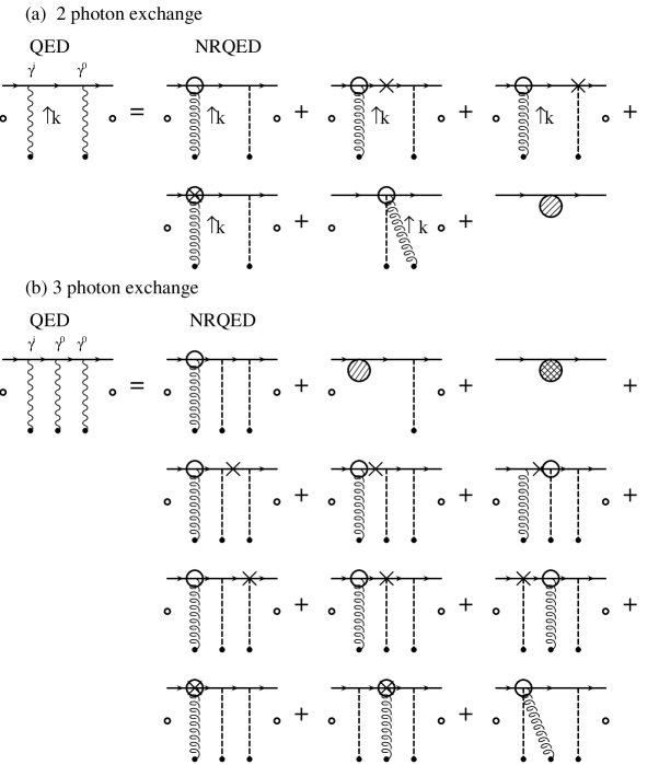
FIG. 1.: Comparison of the QED and NRQED scattering amplitudes. The small circles on the edges of each diagram indicate that a diagram is evaluated on-the-mass-shell and at the threshold external fermions. The shaded circle in (a) is a contact term. The doubly-shaded circle in (b) is a contact term, too. A wavy line is covariant photon in the Feynman gauge, a carly and dashed line are transvers and Coulomb photons, respectively, in the Coulomb gauge. The muon is treated as the static external source and indicated by a dot. For NRQED electron vertices, consult the NRQED Feynman rules given in Ref. [3] .

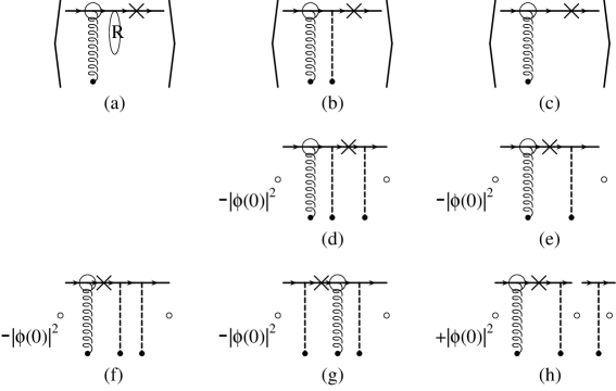
FIG. 2.: Relativistic kinetic term diagrams. The brackets $\langle$  $\rangle$ indicate that the diagram is evaluated with the bound state wave function. The contact term diagram is shown in the right below of the corresponding bound state. The time-reversed diagrams are not shown. R in (a) represents two or more photon exchange part of the Coulomb Green’s function.

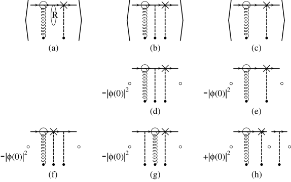
FIG. 3.: Darwin term diagrams.

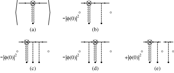
FIG. 4.: Derivative Fermi term diagrams.

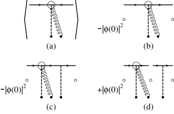
FIG. 5.: Seagull term diagrams.

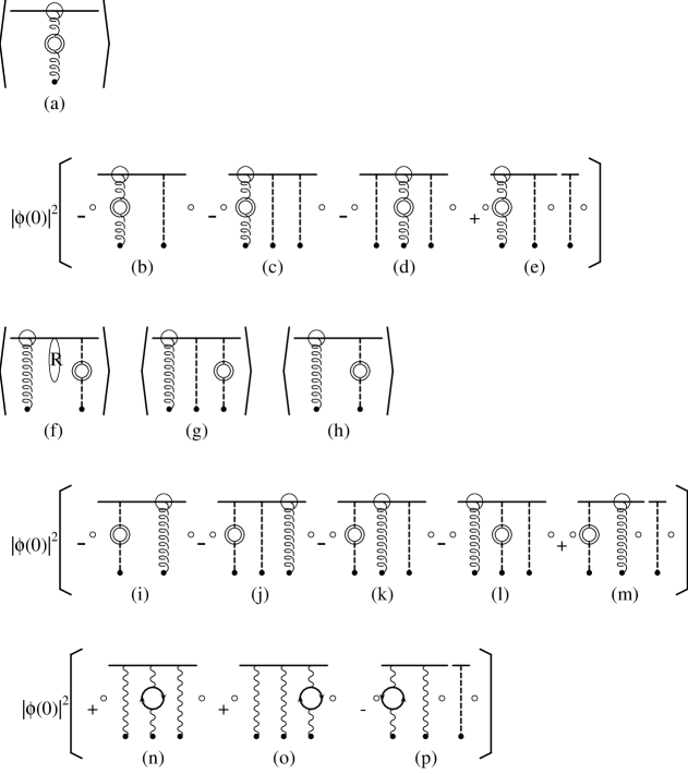
FIG. 6.: Vacuum polarization diagrams contributing to the $\alpha(Z\alpha)^{2}$ correction.

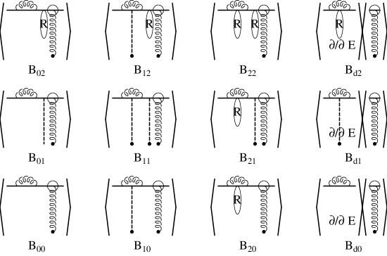
FIG. 7.: Diagrams relevant to the NRQED bound state contibution $E_{B}$ of the $\alpha(Z\alpha)^{2}$ correction.

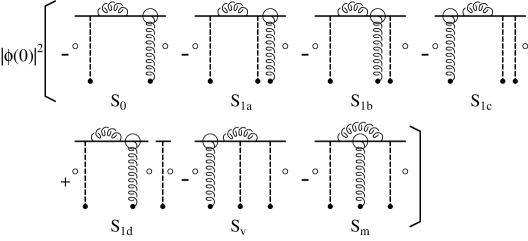
FIG. 8.: Diagrams relevant to the NRQED scattering state contibution $E_{S}$ of the $\alpha(Z\alpha)^{2}$ correction.

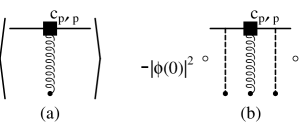
FIG. 9.: Diagrams relevant to the $``$renormalization” constant contibution $E_{R}$ of the $\alpha(Z\alpha)^{2}$ correction. Only the diagrams involving $p^{\prime}p$ interaction term are shown here. For other terms, see Figs. 2,3,4, and 5.

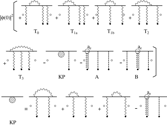
FIG. 10.: Diagrams relevant to the QED scattering state contibution $E_{Q}$ of the $\alpha(Z\alpha)^{2}$ correction. The last line is the difinition of the KP potential which contribute to the $\alpha(Z\alpha)$ correction of the hyperfine splitting.

TABLE I.: Bound state contibutions $E_{B}$ of the $\alpha(Z\alpha)^{2}$ correction from individual diagrams shown in Fig. 7. The overall factor $E_{F}\alpha(Z\alpha)^{2}/\pi$ is omitted.

$\displaystyle\begin{array}[]{ccl}\hline\cr\hline\cr{\rm Diagram}&&~{}~{}~{}~{}~{}~{}~{}~{}~{}~{}~{}~{}{\rm Contribution}\\ \hline\cr B_{00}&&-{16\over 3}\biggl{[}\sqrt{{2\Lambda m\over\gamma^{2}}}-{3\over 4}\ln\biggl{(}{2\Lambda m\over\gamma^{2}}\biggr{)}+{3\over 2}\ln 2-{3\over 4}\biggr{]}\\ \hline\cr B_{01}&&-{16\over 3}\biggl{[}{1\over 4}\ln^{2}\biggl{(}{2\Lambda m\over\gamma^{2}}\biggr{)}+\biggl{(}-\ln 2-{1\over 4}\biggr{)}\ln\biggl{(}{2\Lambda m\over\gamma^{2}}\biggr{)}+{1\over 2}\ln 2+\ln^{2}2+{\pi^{2}\over 6}\biggr{]}\\ \hline\cr B_{02}&&-{16\over 3}\biggl{[}{13\over 8}\ln\biggl{(}{2\Lambda m\over\gamma^{2}}\biggr{)}-{49\over 12}-{13\over 4}\ln 2-{\pi^{2}\over 8}\biggr{]}\\ \hline\cr B_{10}&&{8\over 3}\biggl{[}{1\over 4}\ln^{2}\biggl{(}{2\Lambda m\over\gamma^{2}}\biggr{)}+\biggl{(}-3\ln 2+{1\over 2}\biggr{)}\ln\biggl{(}{2\Lambda m\over\gamma^{2}}\biggr{)}+\ln 2+3\ln^{2}2+{\pi^{2}\over 3}-{3\over 2}\biggr{]}\\ \hline\cr B_{11}&&{8\over 3}\biggl{(}{\pi^{2}\over 6}-{1\over 2}\biggr{)}\biggr{(}\ln\biggl{(}{2\Lambda m\over\gamma^{2}}\biggr{)}-1\biggl{)}-10.499~{}478~{}(61)\\ \hline\cr B_{12}&&{8\over 3}\biggl{(}-{\pi^{2}\over 6}+{9\over 4}\biggr{)}\biggl{(}\ln\biggl{(}{2\Lambda m\over\gamma^{2}}\biggr{)}-1\biggr{)}-5.393~{}042~{}(55)\\ \hline\cr B_{20}&&+0.761~{}648~{}(52)\\ \hline\cr B_{21}&&+0.491~{}192~{}(42)\\ \hline\cr B_{22}&&+0.221~{}861~{}(36)\\ \hline\cr B_{d0}&&-{8\over 3}\biggl{[}{1\over 4}\ln\biggl{(}{2\Lambda m\over\gamma^{2}}\biggr{)}-{1\over 2}\ln 2-{5\over 24}\biggr{]}\\ \hline\cr B_{d1}&&-0.316~{}379~{}(13)\\ \hline\cr B_{d2}&&-0.116~{}135~{}(19)\\ \hline\cr\hline\cr\end{array}$

TABLE II.: Scattering state contributions $E_{S}$ of the $\alpha(Z\alpha)^{2}$ correction from individual diagrams shown in Fig. 8. The overall factor $E_{F}\alpha(Z\alpha)^{2}/\pi$ is omitted. $Li(1/3)=0.366~{}213~{}229~{}\cdots$ is the value of dilogarithmic function $Li(x)$ at $x=1/3$, where $Li(x)=-\int^{x}_{0}dt{\ln(1-t)\over t}$.

$\displaystyle\begin{array}[]{ccl}\hline\cr\hline\cr{\rm Diagram}&&~{}~{}~{}~{}~{}~{}~{}~{}~{}~{}~{}~{}{\rm Contribution}\\ \hline\cr S_{0}&&{16\over 3}\sqrt{{2\Lambda m\over\gamma^{2}}}\\ \hline\cr S_{1a}&&{16\over 3}\biggl{[}{1\over 4}\ln^{2}\biggl{(}{2\Lambda m\over\lambda^{2}}\biggr{)}-\ln 3\ln\biggl{(}{2\Lambda m\over\lambda^{2}}\biggr{)}+{1\over 2}\ln^{2}3+{\pi^{2}\over 4}+Li({1\over 3})\biggr{]}\\ \hline\cr S_{1b}&&{16\over 3}\biggl{[}2\sqrt{{2\Lambda m\over\lambda^{2}}}+\biggl{(}\ln{2\over 3}-1\biggr{)}\ln\biggl{(}{2\Lambda m\over\lambda^{2}}\biggr{)}+{1\over 2}\ln^{2}3+Li({1\over 3})\biggr{]}\\ \hline\cr S_{1c}&&{16\over 3}\biggl{[}2\sqrt{{2\Lambda m\over\lambda^{2}}}+\biggl{(}\ln{2\over 3}-{3\over 2}\biggr{)}\ln\biggl{(}{2\Lambda m\over\lambda^{2}}\biggr{)}+{1\over 2}\ln^{2}3+4\ln 2-{3\over 2}+Li({1\over 3})\biggr{]}\\ \hline\cr S_{1d}&&{16\over 3}\biggl{[}-4\sqrt{{2\Lambda m\over\lambda^{2}}}+3\ln\biggl{(}{2\Lambda m\over\lambda^{2}}\biggr{)}-2\biggr{]}\\ \hline\cr S_{v}&&-{8\over 3}\biggl{[}{1\over 4}\ln^{2}\biggl{(}{2\Lambda m\over\lambda^{2}}\biggr{)}+\biggl{(}-2\ln 2-\ln 3+{1\over 2}\biggr{)}\ln\biggl{(}{2\Lambda m\over\lambda^{2}}\biggr{)}\\ &&~{}~{}+{\pi^{2}\over 4}+5Li({1\over 3})-2\ln^{2}2+{5\over 2}\ln^{2}3+{8\over 3}\ln 2+\ln 3-{7\over 2}\biggr{]}\\ \hline\cr S_{m}&&-{8\over 3}\biggl{[}\biggl{(}-{1\over 2}\ln 3+{1\over 2}\biggr{)}\ln\biggl{(}{2\Lambda m\over\lambda^{2}}\biggr{)}-{\pi^{2}\over 24}+{3\over 2}Li({1\over 3})+{3\over 4}\ln^{2}3-{2\over 3}\ln 2+{1\over 2}\ln 3-1\biggr{]}\\ \hline\cr\hline\cr\end{array}$

TABLE III.: Renormalization constant contributions $E_{R}$ of the $\alpha(Z\alpha)^{2}$ correction from individual diagrams shown in Fig. 9. The overall factor $E_{F}\alpha(Z\alpha)^{2}/\pi$ is omitted.

$\displaystyle\begin{array}[]{ccl}\hline\cr\hline\cr{\rm Diagram}&&~{}~{}~{}~{}~{}~{}~{}~{}~{}~{}~{}~{}{\rm Contribution}\\ \hline\cr\Delta{\cal{E}}_{d}&&\biggl{[}3\ln{2\over 3}-\ln\biggl{(}{\lambda\over\gamma}\biggr{)}\biggr{]}\biggl{[}{8\over 3}\ln\biggl{(}{m\over 2\Lambda}\biggr{)}+{11\over 9}+2a_{e}+a_{e}\biggr{]}\\ \hline\cr\Delta{\cal{E}}_{k}&&\biggl{[}-{1\over 2}-6\ln{2\over 3}+2\ln\biggl{(}{\lambda\over\gamma}\biggr{)}\biggr{]}a_{e}\\ \hline\cr\Delta{\cal{E}}_{s}&&\biggl{[}-{1\over 2}-\ln{2\over 3}-\ln\biggl{(}{\lambda\over\gamma}\biggr{)}\biggr{]}2a_{e}\\ \hline\cr\Delta{\cal{E}}_{q^{2}}&&\biggl{[}{3\over 2}+4\ln 2-3\ln 3\biggr{]}\biggl{[}{4\over 3}\ln\biggl{(}{m\over 2\Lambda}\biggr{)}+{11\over 18}+{1\over 2}a_{e}+{1\over 3}\biggr{]}\\ \hline\cr\Delta{\cal{E}}_{p^{\prime}p}&&\biggl{[}{5\over 8}+{1\over 2}\ln 2-{3\over 4}\ln 3-{1\over 2}\ln\biggl{(}{\lambda\over\gamma}\biggr{)}\biggr{]}a_{e}\\ \hline\cr\hline\cr\end{array}$

TABLE IV.: The QED scattering state contribution $E_{Q}$ for various photon mass $\lambda$. The corresponding diagrams are shown in Fig. 10. The overall factor $E_{F}\alpha(Z\alpha)^{2}/\pi$ is omitted. The uncertainty of $E_{Q}$ is from numerical integration by VEGAS.

$\displaystyle\begin{array}[]{ccccccc}\hline\cr\hline\cr\lambda^{2}/m^{2}&&E_{Q}&&E_{Q}-(E_{Q})_{\rm log}&&{\rm uncertainty}~{}~{}{\rm in}~{}~{}E_{Q}\\ \hline\cr~{}~{}~{}10^{-5}&{}{}{}\hfil&-90.075~{}1&&-8.697~{}1&&0.0024\\ \hline\cr~{}~{}~{}10^{-5.5}&{}{}{}\hfil&-107.943~{}8&&-8.707~{}8&&0.0033\\ \hline\cr~{}~{}~{}10^{-6}&{}{}{}\hfil&-127.575~{}1&&-8.713~{}9&&0.0040\\ \hline\cr~{}~{}~{}10^{-6.5}&{}{}{}\hfil&-148.971~{}3&&-8.717~{}6&&0.0048\\ \hline\cr~{}~{}~{}10^{-7}&{}{}{}\hfil&-172.139~{}0&&-8.725~{}5&&0.0029\\ \hline\cr~{}~{}~{}10^{-7.5}&{}{}{}\hfil&-197.062~{}7&&-8.722~{}0&&0.0030\\ \hline\cr~{}~{}~{}10^{-8}&{}{}{}\hfil&-223.758~{}9&&-8.723~{}7&&0.0026\\ \hline\cr~{}~{}~{}10^{-9}&{}{}{}\hfil&-282.449~{}4&&-8.723~{}4&&0.0016\\ \hline\cr\hline\cr\end{array}$

REFERENCES

- [1] T. Kinoshita and M. Nio, Phys. Rev. Lett. 72, 3803 (1994).
- [2] M. I. Eides and V. A. Shelyuto, Pis’ma v ZhETP 61, 465 (1995) [ JETP Lett. 61 478 (1995)] ; Phys. Rev. A 52, 954 (1995).
- [3] T. Kinoshita and M. Nio, Phys. Rev. D 53, 4909 (1996).
- [4] V. W. Hughes and G. zu Putlitz, Comm. Nucl. Part. Phys. 12, 259 (1984).
- [5] W. E. Caswell and G. P. Lepage, Phys. Lett. B 167, 437 (1986).
- [6] J. R. Sapirstein, private communication, (1995).
- [7] E. Fermi, Z. Phys. 60, 320 (1930).
- [8] A. J. Layzer, Bull. Am. Phys. Soc. 6, 514 (1961); Nuovo Cimento 33, 1538 (1964).
- [9] D. E. Zwanziger, Bull. Am. Phys. Soc. 6, 514 (1961); Nuovo Cimento 34, 77 (1964).
- [10] S. J. Brodsky and G. W. Erickson, Phys. Rev. 148, 26 (1966).
- [11] J. R. Sapirstein, Phys. Rev. Lett. 51, 985 (1983).
- [12] J. R. Sapirstein and D. R. Yennie, in Quantum Electrodynamics, ed. by T. Kinoshita (World Scientific, Singapore,1990), pp. 560 - 672.
- [13] K. Pachucki, Phys. Rev. A 54, 1994 (1996).
- [14] K. Pachucki, Ann. Phys. (NY) 226, 1 (1993).
- [15] G. Breit, Phys. Rev. 35, 1447 (1930).
- [16] T. Kinoshita and G. P. Lepage, in Quantum Electrodynamics , ed. by T. Kinoshita (World Scientific, Singapore,1990), pp.81 - 89.
- [17] G. P. Lepage, L. Magnea, C. Nakhleh, U. Magnea, and K. Hornbostel, Phys. Rev. D 46, 4052 (1992).
- [18] P. Labelle, G. P. Lepage, and U. Magnea, Phys. Rev. Lett. 72, 2006 (1994).
- [19] P. Labelle, preprint McGill/96-33, hep-ph/9608491.
- [20] N. Kroll and F Pollock, Phys. Rev. 84, 594 (1951), Phys. Rev. 86, 876 (1952); R. Karplus, A. Klein, and J. Schwinger, Phys. Rev. 84 597 (1951).
- [21] J. Schwinger, J. Math. Phys. 5, 1606 (1964).
- [22] P. Labelle, private communication (1993).
- [23] D. A. Zwanziger, Phys. Rev. 121, 1128 (1961).
- [24] J. R. Sapirstein, private communication (1995).
- [25] S. J. Brodsky, private communication (1995).
- [26] S. G. Karshenboim, private communication (1995).
- [27] S. M. Schneider, W. Greiner and G. Soff, Phys. Rev. A 50, 118 (1994).
- [28] G. P. Lepage, J. Comput. Phys. 27, 192 (1978).
- [29] W. H. Press, B. P. Flannery, S. A. Teukolsky, and W. T. Vetterling, Numerical Recipes (Cambridge University Press, 1989).
- [30] G. P. Lepage, private communication (1993).
- [31] S. G. Karshenboim, Z. Phys. D 36, 11 (1996).
- [32] H. Persson, et. al. Phys. Rev. Lett. 76, 1433 (1996); P. Sunnergren U. of Goteborg, Ph. D. Thesis (1996).
- [33] S. A. Blundell, K.T. Cheng, and J. Sapirstein, preprint (1996).
- [34] M. Nio and T. Kinoshita, in preparation.
- [35] W. E. Caswell and G. P. Lepage, Phys. Rev. A 18, 810 (1978).