hep-ph/9701399

TTP97–06

January 28, 1997

Flavour Changing Neutral Current Decays of Heavy Baryons:  The Case $\Lambda_{b}\to\Lambda\gamma$

Thomas Mannel and Stefan Recksiegel

Institut für Theoretische Teilchenphysik, D – 76128 Karlsruhe, Germany.

We investigate the rare decay $\Lambda_{b}\to\Lambda\gamma$ which receives both short and long distance contributions. We estimate the long distance contributions and find them very small. The form factors are obtained from $\Lambda_{c}\to\Lambda\ell\bar{\nu}_{\ell}$ using heavy quark symmetry and a pole model. The short distance piece opens a window to new physics and we discuss the sensitivity of $\Lambda_{b}\to\Lambda\gamma$ to such effects.

1 Introduction

Flavour Changing Neutral Current (FCNC) processes have attracted renewed attention since the recent CLEO measurement of the FCNC decays of the type $b\to s\gamma$. In the Standard Model (SM) these processes are forbidden at the tree level and are strongly suppressed by the GIM mechanism, in particular for up type quarks. Hence they offer a unique possibility to test the CKM sector of the SM and possibly open a window to physics beyond the SM.

From the experimental side there is some data on the exclusive decay $B\to K^{*}\gamma$ and the inclusive decay $B\to X_{s}\gamma$ with branching fractions [1]

$$Br(B^{+}\to K^{+*}\gamma) = (5.7\pm 3.3)\times 10^{-5}$$

$$Br(B^{0}\to K^{0*}\gamma) = (4.0\pm 1.9)\times 10^{-5}$$

$$Br(B\to X_{s}\gamma) = (2.3\pm 0.7)\times 10^{-4}$$

which is at present compatible with the SM. However, the experimental as well as the theoretical uncertainties are still sizable; in particular an improvement of the theoretical prediction involves a next-to-leading order calculation which has recently become available [2].

Various scenarios have been used to calculate the influence of physics beyond the SM on the decay $b\to s\gamma$ and also model independent analyses have been suggested [3]. However, based on the decays of $B$ mesons it will not be possible to analyse the helicity structure of the effective hamiltonian mediating the decay $b\to s\gamma$, since the information on the handedness of the quarks is lost in the hadronization process.

The only way to access the helicity of the quarks is to consider the decay of baryons. From the experimental side the decay $\Lambda_{b}\to\Lambda\gamma$ is a good candidate, since the subsequent $\Lambda$ decay $\Lambda\to p\pi$ is self analyzing. The only experimental drawback of this mode is that the production rate of $\Lambda_{b}$ baryons in $b$ quark hadrionization is about an order of magnitude smaller than the rate for $B$ mesons, and hence the analysis suggested here has to wait for more data on heavy quark decays from colliders.

From the theoretical point of view one may make use of the heavy quark symmetry for the $b$ quark. The $b\to s$ transition is of the heavy-to-light type for which heavy quark symmetries restrict the number of form factors for the baryonic transition $\Lambda_{Q}\to$ light spin-1/2 baryon to only two. These heavy quark symmetries are expected to work best at the point of maximal momentum transfer $q=q_{max}$ (corresponding to small recoil to the light degrees of freedom), whereas in the decay under consideration we are at the opposite side of phase space, namely at $q^{2}=0$. We shall still use heavy quark symmetry, at least it will be a reasonable model assumption for the form factors. Once we use heavy quark symmetries over the whole phase space, one may obtain the form factors from the semileptonic decay $\Lambda_{c}\to\Lambda\ell\bar{\nu}_{\ell}$, for which some data exists [4]. Unfortunately, data are still not good enough to allow a measurement of the two form factors as a function of $q^{2}$, and consequently one has to model the form factor shape using some ansatz. This makes the predicted total rate to some extent uncertain, while the polarization of the $\Lambda$ is practically unaffected by the choice of a model.

Another theoretical difficulty with the process suggested are possible long distance contributions which will dilute the effects of a non-SM-contribution to the short distance effective hamiltonian for $b\to s\gamma$. There are two effects of this kind: A vector dominance contribution from the process $b\to s(\bar{c}c)\to sJ/\Psi\to s\gamma$ and the internal $W$ exchange. Both contributions are hard to estimate, since one has to refer to models.

In the next section we shall discuss the short distance contribution and its hadronic matrix elements. In section 3 we shall use simple models to estimate the long distance contributions. In section 4 we shall use the input of the semileptonic $\Lambda_{c}$ decay and two simple models for the form factors to obtain a prediction for the total rate of $\Lambda_{b}\to\Lambda\gamma$. Section 5 is devoted to a discussion of the polarization variable and its connection to the parameters of the short distance part of the effective hamiltonian. The standard model and the sensitivity to non-standard model effects are considered. Finally we discuss our results and conclude.

2 The short distance contribution

In the SM as well as in many non-SM scenarios, the hamiltonian relevant for $b\to s$ transitions consists of ten operators ${\cal O}_{i},i=1,...10$, of which only one (${\cal O}_{7}$) mediates the decay $b\to s\gamma$. The effective hamiltonian has the form

$$H_{eff}=\frac{4G_{F}}{\sqrt{2}}V_{ts}^{*}V_{tb}C_{7}(\mu){\cal O}_{7}(\mu)$$ (1)

with

$${\cal O}_{7}=\frac{e}{32\pi^{2}}\left[m_{b}\bar{s}\sigma_{\mu\nu}(1+\gamma_{5})b+m_{s}\bar{s}\sigma_{\mu\nu}(1-\gamma_{5})b\right]F^{\mu\nu}$$ (2)

where the renormalization scale $\mu$ is usually taken to be $m_{b}$. It is well known that the leading-log calculation exhibits a strong residual dependence on the renormalization point $\mu$, since the QCD corrections encoded in $C_{7}$ are sizable. Recently the complete next-to-leading order calculation has been performed and we shall use the value for $C_{7}$ from this calculation.

A more general form of the Operator ${\cal O}_{7}$ allowing for non–SM couplings is

$$\widehat{\cal O}_{7}=\frac{e}{32\pi^{2}}m_{b}\bar{s}\sigma_{\mu\nu}(g_{V}-g_{A}\gamma_{5})bF^{\mu\nu}$$ (3)

where $g_{V}$ and $g_{A}$ are the vector and axial vector couplings, respectively. In the Standard Model

$$g_{V}=1+{m_{s}\over m_{b}},\quad g_{A}=-1+{m_{s}\over m_{b}}$$ (4)

The correction to the integer values of $g_{A}$ and $g_{V}$ due to the non-vanishing $s$ quark mass is of the order of 3%.

Hence in general at the level of dimension-six operators there are two operators relevant for the decay under discussion, namely the one with right-handed $b$ quark (implying left-handed $s$ quark) and the one with right-handed $s$ quark (implying left-handed $b$ quark). In other words, in general there are two parameters, which may be taken to be $C_{7}g_{V}$ and $C_{7}g_{A}$.

Once the short distance structure of the effective Hamiltonian is known, it remains to calculate matrix elements of the operators. In the present case we shall make use of the fact that the $b$ quark is heavy, while the $s$ quark is taken to be a light quark. In general, heavy quark symmetries restrict the number of possible form factors quite significantly; in the present case there are only two, parametrized by [6]

$$\left<\Lambda(p,s)|\bar{s}\Gamma b|\Lambda_{b}(v,s^{\prime})\right>=\bar{u}_{\Lambda}(p,s)\{F_{1}(p.v)+\mathchoice{\ooalign{$\hfil\displaystyle\mkern 0.0mu/\hfil$\crcr$\displaystyle v$}}{\ooalign{$\hfil\textstyle\mkern 0.0mu/\hfil$\crcr$\textstyle v$}}{\ooalign{$\hfil\scriptstyle\mkern 0.0mu/\hfil$\crcr$\scriptstyle v$}}{\ooalign{$\hfil\scriptscriptstyle\mkern 0.0mu/\hfil$\crcr$\scriptscriptstyle v$}}F_{2}(p.v)\}\Gamma u_{\Lambda_{b}}(v,s^{\prime})$$ (5)

where $v$ is the velocity of the heavy $\Lambda_{b}$–baryon which in HQET is equal to the velocity of the heavy $b$–quark, $s^{\prime}$ is the spin of the heavy $\Lambda_{b}$, which due to heavy quark spin symmetry equals the spin of the $b$ quark, $p$ is the momentum of the $\Lambda$–baryon and $s$ its spin. Furthermore, $\Gamma$ is an arbitrary Dirac matrix, such that any transition between a $\Lambda_{Q}$ ($Q=b,c$) and a light spin $1/2$ baryon is given by the same form factors. In particular, this allows us to compare the exclusive semileptonic decay of a $\Lambda_{c}$ with the process under consideration here, although the helicity structure of the relevant currents is completely different.

Heavy quark symmetries are expected to work best at the point where the final state light hadron is slow (in the rest frame of the decaying hadron), such that the momentum transfer to the light degrees of freedom is small. At the other end of phase space, $q^{2}=0$, it is easy to see that the the momentum transfer to the light degrees of freedom scales with the mass of the heavy quark, it is not clear whether heavy quark symmetries are applicable at this point. However, we shall still make use of heavy quark symmetries even for $q^{2}=0$, taking this in the worst case as a model assumption. Keeping this in mind, the matrix element of the operator $O_{7}$ between the initial and final state is

$$\langle\Lambda(p,s),\gamma(k,\varepsilon)|O_{7}|\Lambda_{b}(v,s^{\prime})\rangle$$ (6)

$$\qquad={e\over 16\pi^{2}}m_{b}\langle\Lambda(p,s)|\bar{s}\sigma_{\mu\nu}{1\over 2}(g_{V}-g_{A}\gamma_{5})b|\Lambda_{b}(v,s^{\prime})\rangle\langle\gamma(k,\varepsilon)|F^{\mu\nu}|0\rangle$$

The quantity of interest is the decay rate of unpolarized $\Lambda_{b}$ baryons into $\Lambda$ baryons with a definite spin directions $s$. To obtain from this expression this rate as a function of the form factors taken at $q^{2}=0$ is a matter of algebra, and we obtain

$$\Gamma = {C_{7}^{2}G_{F}^{2}\over\pi}(V_{ts}^{*}V_{tb})^{2}({e\over 16\pi^{2}})^{2}m_{b}^{2}m_{\Lambda_{b}}^{3}(1-x^{2})$$ (7)

$$\{{g_{V}^{2}+g_{A}^{2}\over 2}[(1-2x^{2}+x^{4})|F_{1}|^{2}$$

$$\quad+(x-2x^{3}+x^{5})(F_{1}F_{2}^{*}+F_{1}^{*}F_{2})$$

$$\quad+(x^{2}-2x^{4}+x^{6})|F_{2}|^{2}]$$

$$+g_{V}g_{A}(v.s)[(2x-2x^{3})|F_{1}|^{2}$$

$$\quad+(2x^{2}-2x^{4})(F_{1}F_{2}^{*}+F_{1}^{*}F_{2})$$

$$\quad+(2x^{3}-2x^{5})|F_{2}|^{2}]\}$$

where $x=m_{\Lambda}/m_{\Lambda_{b}}$.

As expected, the terms which depend on the spin of the $\Lambda$ are all proportional to $|C_{7}|^{2}g_{V}g_{A}$, while the rest of the rate has the factor $|C_{7}|^{2}(g_{V}^{2}+g_{A}^{2})/2$. Thus a polarization analysis of the final state $\Lambda$ allows a determination of the ratio $g_{A}/g_{V}$.

In order to comply with the standard definitions we rewrite the rate in terms of the polarization variables as defined in [1]

$$\Gamma=\Gamma_{0}\cdot[1+\alpha^{\prime}{\rm{\bf\hat{p}.S}_{\Lambda}}]$$ (8)

where ${\rm\bf\hat{p}}$ is the momentum vector of the $\Lambda$ and ${\rm{\bf S}_{\Lambda}}$ is its spin vector. Using expression (7) one finds for $\alpha^{\prime}$

$$\alpha^{\prime} = {(1-x^{2})\over(1+x^{2})}{(2x-6x^{3})+2(2x^{2}-6x^{4})R+2x^{3}R^{2}\over(1-2x^{2}+x^{4})+2(x-2x^{3})R_{(}x^{2}-2x^{4})R^{2}}{2g_{V}g_{A}\over g_{V}^{2}+g_{A}^{2}}$$ (9)

$$= 0.378\cdot{2g_{V}g_{A}\over g_{V}^{2}+g_{A}^{2}}$$ (10)

where we have only used the central value of the CLEO measurement [7]

$$R={F_{2}\over F_{1}}=-0.25\pm 0.14\pm 0.08$$ (11)

and the ratio of the baryon masses $x=0.20$.

Note that $\alpha^{\prime}$ vanishes in the limit $m_{\Lambda}\to 0$; the leading order is given by

$$\alpha^{\prime}=2x{2g_{V}g_{A}\over g_{V}^{2}+g_{A}^{2}}$$ (12)

which for $x=0.2$ already is a reasonable approximation to the value obtained from (10).

3 Long Distance Contributions

In order to obtain a realistic estimate of the branching ratio and of the sensitivity on the coupling constants $g_{V}$ and $g_{A}$ one also has to take into account the long distance contributions. One may distinguish between two types of contributions: the vector-meson-dominance like contributions, where there is a vector meson intermediate state and the internal $W$-boson exchange, which corresponds to the weak transition of the heavy $\Lambda_{b}$ into excited $\Lambda$ states decaying subsequently into $\Lambda$ and a photon.

The vector-dominance like contributions are dominated by the CKM allowed contributions where one has a $J/\Psi$ as the internal vector meson. They are governed by a different part of the $\Delta B=1$ hamiltonian given by

$$H_{\rm eff}^{c\bar{c}}={G_{F}\over\sqrt{2}}V_{cs}^{*}V_{cb}(C_{1}{\cal O}_{1}+C_{2}{\cal O}_{2})$$ (13)

with

$${\cal O}_{1} = (\bar{s}_{\alpha}\gamma_{\mu}(1-\gamma_{5})b_{\alpha})(\bar{c}_{\beta}\gamma^{\mu}(1-\gamma_{5})c_{\beta}),$$ (14)

$${\cal O}_{2} = (\bar{s}_{\alpha}\gamma_{\mu}(1-\gamma_{5})b_{\beta})(\bar{c}_{\beta}\gamma^{\mu}(1-\gamma_{5})c_{\alpha}),$$ (15)

where $\alpha$ and $\beta$ are $SU(3)_{color}$ indices and $C_{1}$ and $C_{2}$ are the corresponding Wilson coefficients.

The decays $\Lambda_{b}\to\Lambda\Psi^{(n)}$ ($\Psi^{(n)}$ being the excited states with the quantum numbers of the $J/\Psi$) are exclusive non-leptonic decays and the result for this part will be strongly dependent on model assumptions. Following the usual folklore we keep from ${\cal O}_{2}$ only the part in which $c$ and $\bar{c}$ are in a color singlet state and perform factorization with this part. Thus we model $\Lambda_{b}\to\Lambda\Psi^{(n)}$ by

$$\langle\Lambda\Psi^{(n)}|H_{\rm eff}^{c\bar{c}}|\Lambda_{b}\rangle={G_{F}\over\sqrt{2}}V_{cs}^{*}V_{cb}\left(C_{1}+\frac{C_{2}}{N_{c}}\right)\langle\Lambda|\bar{s}\gamma_{\mu}(1-\gamma_{5})b|\Lambda_{b}\rangle\langle\Psi^{(n)}|(\bar{c}\gamma^{\mu}(1-\gamma_{5})c|0\rangle$$ (16)

It is well known that the combination of Wilson coefficients $C_{1}+C_{2}/N_{c}$ ($N_{c}=3$) comes out very small due to an accidental cancellation between the two contributions, yielding a too small rate for e.g. the decay $B\to KJ/\Psi$. Hence it is more realistic to use for this combination the value implied by the data and to put $a_{2}=C_{1}+C_{2}/N_{c}=0.24\pm 0.04$ [8].

Furthermore, we consider a process in which we are dealing with a virtual $\Psi^{(n)}$ which is quite far off shell. It has been suggested [8] to take into account this effect by assuming a $q^{2}$ dependent decay constant for the $\Psi^{(n)}$ according to

$$\langle\Psi^{(n)}(q,\epsilon)|\bar{c}\gamma^{\mu}(1-\gamma_{5})c|0\rangle=ig_{\Psi}^{(n)}(q^{2})\epsilon^{*}_{\mu}(q)$$ (17)

From the comparison between the leptonic width of the $J/\Psi$ (yielding $g_{\Psi}(m_{\Psi}^{2})$) with the data from $\Psi$-photo-production (yielding $g_{\Psi}(0)$) one obtains the ratio

$$\kappa_{\Psi}=\frac{g_{\Psi}(0)}{g_{\Psi}(m_{\Psi}^{2})}=0.12\pm 0.04$$ (18)

corresponding to a suppression by roughly a factor of ten. Unfortunately, there is no data for excited $\Psi$’s, so we shall simply assume the same suppression factor $\kappa$ for all of them.

Assembling all the pieces, summing over all $\Psi$ resonances with the appropriate quantum numbers and employing the Gordon identity to isolate the transverse part one finds

$$\langle\Lambda\gamma|H_{\rm eff}^{c\bar{c}}|\Lambda_{b}\rangle=-{1\over 3}a_{2}\kappa\sum_{n}{g_{\Psi^{(n)}}^{2}(m_{\Psi^{(n)}}^{2})\over m_{\Psi^{(n)}}^{2}m_{b}}\langle\Lambda\gamma|\bar{s}\sigma_{\mu\nu}(1+\gamma_{5})b|\Lambda_{b}\rangle\langle\gamma|F^{\mu\nu}|0\rangle.$$ (19)

which takes the same form as the short distance contribution.

The second kind of long distance contribution is the one originating from internal $W$ exchange. The relevant Feynman diagrams are depicted in fig.1.

Figure 1: Internal $W$ exchange

This contribution is even more difficult to calculate and we shall perform a relatively crude estimate. The idea we are going to employ is along the lines of Brodsky and Lepage [9]. In this picture the decay amplitude is decomposed into a hard piece which is calculated in terms of perturbative QCD while the soft contribution is described in terms of wave functions.

Since in this picture a baryon is still a relatively complicated object, we shall simplify further by gathering the up and the down quark in the $\Lambda_{b}$ and the down and strange quark of the $\Lambda$ into diquarks. This picture is in fact to some extent motivated from the phenomenological side, since it has been advertised as an explanation of the $\Delta I=1/2$ rule in hyperon decays [10].

Hence we shall describe the baryons effectively as a bound state of a diquark and a $b$ quark or an $u$ quark, respectively. The hard process in the sense of Brodsky and Lepage is a $b\to u$ transition in which the weak boson is absorbed by the $(ud)$ diquark, transforming it into a $(sd)$ diquark. In order to conserve energy and momentum a photon is radiated off, making this in total a $\Lambda_{b}\to\Lambda\gamma$ transition.

Figure 2: Feynman rules for diquarks

To perform the calculation one has to define Feynman rules for the radiation and the weak transition of the diquarks, which are simply obtained from the corresponding interactions of scalar particles in a straightforward way. Note that in order to ensure gauge invariance one also has to include a “seagull” term corresponding to a diquark-$W$-$\gamma$ coupling. The Feynman rules are given in fig.2 and these allow us a calculation of the hard part of the decay amplitude.

The soft contributions are parametrized in terms of wave functions of the two constituents of the baryons. In the spirit of [9] we neglect the transverse components of the momenta of the constituents. The $\Lambda_{b}$ is moving with the velocity $v$ and hence we write for the for the momentum $p$ of the $b$ quark $p=xm_{b}v$ and $k=(1-x)m_{b}v$ for the momentum of the $(ud)$ diquark. Similarly, we have $p^{\prime}=y(m_{b}v-q)$ for the momentum of the $u$ quark in the $\Lambda$ and $k^{\prime}=(1-y)(m_{b}v-q)$ for the momentum of its $(ds)$ diquark. The wave functions describing the soft part are $\Phi(x)$ and $\phi(y)$ for the $\Lambda_{b}$ and the $\Lambda$, which are functions of the momentum fractions $x$ and $y$. For the $\Lambda_{b}$ we assume that the $b$ quark carries almost all momentum, which means that $x$ fiffers from one only by terms of the order $1/m_{b}$, such that $k$ is independent of $m_{b}$ in the heavy mass limit. Hence we use

$$\Phi(x)={1\over 2\sqrt{3}}f_{B}\delta(1-x)$$ (20)

for the wave functon of the $\Lambda_{b}$.

For the $\Lambda$ all the quarks have comparable masses and we use a simple Ansatz such that the average of $y$ is $1/3$. Motivated by the corresponding ansatz for the pion wave function we use

$$\phi(y)=2\sqrt{3}f_{\pi}y(y-1)^{2}$$ (21)

where we have assumed that the analogue of the decay constant is simply $f_{\pi}$.

Using this picture for the internal $W$ exchange it turns out that its contribution is much smaller than the long distance contribution of the vector dominance type. This is not a surprise, since the internal $W$ exchange is on one hand suppressed by the small combination $V_{ub}V_{us}^{*}$ of CKM elements, on the other hand it contains two decay constants $f_{\pi}$ and $f_{B}$, yielding another suppression by a factor $f_{\pi}f_{B}/m_{b}^{2}$

In total, in the way we have estimated the long distance contributions they turn out to be small, such that the decay $\Lambda_{b}\to\Lambda\gamma$ is dominated by the short distance piece, which may be sensitive to new physics.

Quantitatively, the long distance corrections are dominated by the vector-dominance contribution. Summing over the lowest six $\Psi^{(n)}$ we find that the long distance contributions may be absorbed into a redefinition of the coupling constants $g_{A}$ and $g_{V}$ according to

$$\hat{g_{V}}=g_{V}+\rho\quad\mbox{and}\quad\hat{g_{A}}=g_{A}-\rho,\quad\mbox{where}\quad\rho=0.035$$ (22)

4 Form Factors form the Semileptonic Decay $\Lambda_{c}\to\Lambda\ell\bar{\nu}_{\ell}$

Since we are dealing with an exclusive decay, we eventually need some input for the form factors in order to calculate numbers. However, not much is known about these functions, except that they have to obey the heavy quark symmetry implied by the heavy-to-light transition we are considering. In particular, at least at maximum momentum transfer the form factors appearing in $\Lambda_{b}\to\Lambda$ transition and $\Lambda_{c}\to\Lambda$ decays have to be the same, independent of the spin structure of the currents involved, see (5).

Again we shall assume heavy quark symmetry over all phase space including $q^{2}=0$ in $\Lambda_{b}\to\Lambda$ and extract the relevant form factors from $\Lambda_{c}\to\Lambda\ell\bar{\nu}_{\ell}$, which is according to (5) given by the same two form factors as $\Lambda_{b}\to\Lambda\gamma$. For the semileptonic $\Lambda_{c}$ decay there is some experimental data [7]; the total rate and the form factor ratio $\left<F_{2}/F_{1}\right>$ has been measured, where the brackets indicate a particular average over phase space.

Nothing is known about the $q^{2}$ dependence of the form factors and at that point model assumptions enter the game. We shall start from a simple pole model for both form factors

$$F_{1/2}(q^{2})=F^{\rm max}_{1/2}\cdot\left({M_{1/2}^{2}-m_{Q}^{2}\over M_{1/2}^{2}-q^{2}}\right)^{n},\quad n=1,2\,,$$ (23)

where $M_{1/2}$ is the mass of the nearest resonance with the correct quantum numbers for $F_{1}$ and $F_{2}$ rspectively and $F^{\rm max}_{1/2}$ is a normalization factor. The form factors in (5) are given in terms of the energy $p.v$ of the outgoing light baryon which has a simple relation with the momentum transfer $q^{2}=m_{Q}^{2}+m_{\Lambda}^{2}-2m_{Q}(p.v)$. Inserting this into the denominator of our form factor parametrization we have

$$M_{1/2}^{2}-q^{2}=M_{1/2}^{2}+2m_{Q}(p.v)-m_{Q}^{2}-m_{\Lambda}^{2}\approx M_{1/2}^{2}+2m_{Q}(p.v)-m_{Q}^{2}$$ (24)

where we have neglected the mass of the light baryon. The relevant resonances contain a heavy quark and some light degrees of freedom and hence the mass of the resonance is $M_{1/2}=m_{Q}+\Lambda_{1/2}$, where we shall in the following identify $\Lambda_{1}=\Lambda_{2}=\Lambda$. The parameter $\Lambda$ is small compared to the heavy quark mass and does not scale with the heavy mass; it remains a constant as $m_{Q}\to\infty$. Using this the denominator of the pole fomula for the form factors becomes

$$M_{1/2}^{2}-q^{2}=(m_{Q}+\Lambda)^{2}+2m_{Q}(p.v)-m_{Q}^{2}\approx 2m_{Q}(\Lambda+(p.v))$$ (25)

For the $\Lambda_{c}\to\Lambda$ transition the relevant resonance for the vector current is the $D_{s}^{*}$ and since in the heavy mass limit $m_{c}\sim m_{\Lambda_{c}}$, we have $\Lambda\approx m_{\Lambda_{c}}-m_{D_{s}^{*}}=175$ MeV, while for the bottom decay $\Lambda_{b}\to\Lambda$ we have the $B_{s}^{*}$ in the vector channel, and hence here we obtain $m_{\Lambda_{b}}-m_{B_{s}^{*}}=225$ MeV. Thus we have a fairly consistent picture and shall use $\Lambda=200$ MeV, it turns out that the dependence of our results on $\Lambda$ is weak.

Putting the pieces together we use as a parametrization of the form factors in the heavy mass limit

$$F_{1/2}(p.v)=N_{1/2}\cdot\left({\Lambda\over\Lambda+p.v}\right)^{n},\quad n=1,2\,,$$ (26)

whre we assume for simplicity the same $(p.v)$ dependence for both form factors. In this simple case the ratio of the form factors $R=F_{2}/F_{1}$ is independent of $(p.v)$ and we may use the value measured by CLEO without worrying about the phase space average going into the measurement. We shall use [7]

$$R=F_{2}/F_{1}=N_{2}/N_{1}=-0.25\pm 0.14\pm 0.08$$ (27)

The large uncertainty in this value does not imply a large uncertainty in our results since any appearance of the form factor $F_{2}$ is suppressed by a factor $m_{\Lambda}/m_{\Lambda_{Q}}$.

Using the measured branching ratio for $\Lambda_{c}\to\Lambda e^{+}\nu$ and the lifetime of $\Lambda_{c}$ from [1] one obtains the normalization $N_{1}$

$$|N_{1}|=7.06\mbox{\quad(monopole)\quad\mbox{and} \quad}|N_{1}|=52.32\mbox{\quad(dipole)}$$ (28)

Using the pole formulae (26) for the extrapolation to $q^{2}=0$ in the decay $\Lambda_{b}\to\Lambda\gamma$ we obtain for the form factors

$$F_{1}(q^{2}=0)=0.45\mbox{\quad(monopole)\quad bzw. \quad}F_{1}(q^{2}=0)=0.22\mbox{\quad(dipole)}.$$ (29)

This may be inserted into (7) with the corrections from (22) to obtain the total rate for the decay $\Lambda_{b}\to\Lambda\gamma$ in the standard model.

In the heavy mass limit the mass of the $\Lambda_{b}$ is equal to the $b$ quark mass and hence the total rate depends on $m_{b}^{5}$, where some of the mass dependence comes from phase space (and is actually $m_{\Lambda_{b}}$) and some is due to the $m_{b}$–dependence of the effective hamiltonian. To get rid of this $m_{b}^{5}$–dependence we take as a reference the inclusive semileptonic decays of the $B$ meson and write:

$${\Gamma(\Lambda_{b}\rightarrow\Lambda\gamma)\over\Gamma(B\rightarrow X_{c}l\nu)}={BR(\Lambda_{b}\rightarrow\Lambda\gamma)\over BR(B\rightarrow X_{c}l\nu)}\cdot{\Gamma_{\rm tot}(\Lambda_{b})\over\Gamma_{\rm tot}(B)}$$ (30)

The inclusive semileptonic decay rate of $B$ mesons depends also on $m_{b}^{5}$ and is given by

$$\Gamma(B\rightarrow X_{c}l\nu)={m_{b}^{5}G_{F}^{2}V_{cb}^{2}\over 192\pi^{3}}\,\eta_{\rm QCD}\,r_{c},$$ (31)

where $\eta_{\rm QCD}=0.94$ is a QCD correction and $r_{c}=0.45$ is a phase space factor.

Using the lifetimes and the inclusive semileptonic branching fraction $BR(B\rightarrow X_{c}l\nu)=(10.3\pm 1.0)\%$ from [1] we obtain

$$BR(\Lambda_{b}\rightarrow\Lambda\gamma)=(1-4.5)\cdot 10^{-5},$$ (32)

where the lower and upper value corresponds to a dipole and monopole $q^{2}$ evolution of the form factors, respectively.

For values of $g_{A}$ and $g_{V}$ different from the standard model ones one has to multiply the above equation by the factor $(g_{A}^{2}+g_{V}^{2})/2$, neglecting the strange quark mass and the long distance contributions.

5 $\Lambda_{b}\to\Lambda\gamma$ as a Test of the Standard Model

In this section we shall discuss the possibility of using the decay $\Lambda_{b}\to\Lambda\gamma$ as a test of the Standard model and to what extent it could be a possible window to new physics.

As opposed to its mesonic counterpart, the decay $B\to K^{*}\gamma$, the baryonic rare decay $\Lambda_{b}\to\Lambda\gamma$ allows access to the helicity structure of the short distance piece of the effective hamiltonian, since the helicity of the final state $\Lambda$ can be measured. The two relevant dimension-5 operators entering the short distance part are parametrized in terms of two coupling constants $C_{7}g_{A}$ and $C_{7}g_{V}$ and the polarization of the final state $\Lambda$ is sensitive to these couplings.

The first piece of information is the total rate of $\Lambda_{b}\to\Lambda\gamma$ which contains (as does the mesonic decay $B\to K^{*}\gamma$) information on the combination $(g_{V}C_{7})^{2}+(g_{A}C_{7})^{2}$, while the polarization variable $\alpha$ defined in (10) contains information on $(C_{7}g_{A})/(C_{7}g_{V})$.

As we have discussed above, our rough estimates of the long distance contributions indicate that they are very small and will not significantly influence the sensitivity of the $\alpha^{\prime}$ measurement on the parameters of the short distance part of the effective hamiltonian.

In the following we shall use the measurement of the inclusive rate $B\to X_{s}\gamma$ to fix $(g_{V}C_{7})^{2}+(g_{A}C_{7})^{2}$; in the $C_{7}g_{V}$–$C_{7}g_{A}$–plane a measurement of any total rate (meaning any of the processes $B\to X_{s}\gamma$, $B\to K^{*}\gamma$ or $\Lambda_{b}\to\Lambda\gamma$) will correspond to a circle, since all these decay rates are proportional to $(g_{V}C_{7})^{2}+(g_{A}C_{7})^{2}$.

If in future experiments a measurement of $\alpha^{\prime}$ in $\Lambda_{b}\to\Lambda\gamma$ is performed one may use the relation between $\alpha^{\prime}$ and $(C_{7}g_{A})/(C_{7}g_{V})$. Including our estimate of the long distance contributions, one obtains

$$C_{7}g_{A}=(C_{7}g_{V}+C_{7}\rho)\left(\frac{0.353}{\alpha^{\prime}}\pm\sqrt{\left(\frac{0.353}{\alpha^{\prime}}\right)^{2}-1}\right)+C_{7}\rho$$ (33)

which corresponds to straight lines in the $C_{7}g_{A}$–$C_{7}g_{V}$ plane. Neglecting the long distance contribution (i.e. $\rho=0$) these lines would go through the origin; including our estimate for these long distance contributions we also need an input for the Wilson coefficient $C_{7}$, for which we shall use the standard model value as obtained form the NLLO calculation in [2].

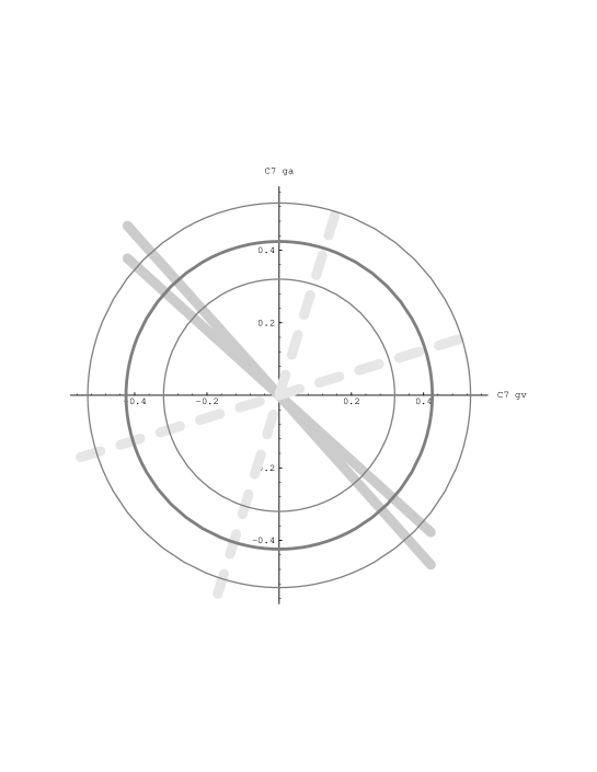
Figure 3: The $C_{7}g_{A}$–$C_{7}g_{V}$ plane

In fig.3 we plot the $C_{7}g_{A}$–$C_{7}g_{V}$ plane. The central circle corresponds to the central value of the measurement of $B\to X_{s}\gamma$ and the thin circles indicate the experimental uncertainty. Assuming the standard model values for $C_{7}g_{A}$ and $C_{7}g_{V}$ we have also plotted the corresponding lines. The width of these lines is given by our estimate for the long distance contributions; we have taken this estimate as an additional uncertainty meaning that the width of these lines is $2\rho C_{7}$.

A measurement of $\alpha^{\prime}$ yields in general two lines which have in total four intersections with the circle. The two intersections of each line correspond to a sign interchange $g_{A}\to-g_{A}$ and at the same time $g_{V}\to-g_{V}$ which is an unobservable phase. The remaining ambiguity corresponds to the interchange $g_{A}\to g_{V}$ and $g_{V}\to g_{A}$, since the polarization variable and the total rate are symmetric functions of $g_{A}$ and $g_{V}$. Graphically this means that the two lines for a measured value of $\alpha^{\prime}$ are mirror images of each other with respect to the lines $g_{A}=|g_{V}|$. In order to resolve this ambiguity additional measurements would be necessary.

In the SM $|g_{A}|\approx|g_{V}|$ ($\alpha^{\prime}=-0.351$) up to corrections from the not-vanishing $s$ quark mass, therefore the two solid lines almost coincide for the SM value of $\alpha^{\prime}$. We also have plotted two dashed lines for a hypothetical measurement of $\alpha^{\prime}=0.2$.

6 Conclusions

With the advent of the second generation $b$ physics experiments, bottom baryons will provide a wealth of additional information on $b$ quarks. In particular, specific aspects of FCNC decays can be tested which are not accessible in $B$ mesons decays.

As its mesonic counterpart, $\Lambda_{b}\to\Lambda\gamma$ is dominated by the short distance part of the effective hamiltonian, although there are additional long distance effects such as internal $W$ exchange. We have estimated the long distance effects using standard methods and found a negligibly small contribution.

Thus one expects a good sensitivity to test the short distance part, the relevant piece of which is given in terms of two operators, which differ by the handedness of the $b$ quark. It is a particular property of the decays of the $\Lambda_{b}$ that they allow one to test the handedness of the effective interaction; this is impossible in the corresponding meson decays.

Heavy quark symmetries imply relations between the form factors which are thought to hold best close to the point where the outgoing hadron is almost at rest. For the transition $\Lambda_{b}\to$ light spin-1/2 baryon there are only two independent form factors due to heavy quark symmetry. Measuring these form factors in $\Lambda_{c}\to\Lambda\ell\bar{\nu}_{\ell}$ then allows us to predict other processes. Unfortunately, in the process $\Lambda_{b}\to\Lambda\gamma$ we are considering the end of the $q^{2}$ spectrum, where the $\Lambda$ receives a large recoil of the order of the $b$ quark mass, and hence heavy quark symmetries might fail. We still used the relations implied by them, which in the worst case is simply a model assumption.

Using the input for the form factors obtained from $\Lambda_{c}\to\Lambda\ell\bar{\nu}_{\ell}$ we made predictions for the decay $\Lambda_{b}\to\Lambda\gamma$ within the standard model and beyond. It turns out that a measurement of the polarization of the final state $\Lambda$ is quite sensitive to the handedness of the underlying effective short distance hamiltonian, up to a twofold ambiguity, which cannot be resolved by a measurement of the rate and the polarization alone.

With a branching ratio for $\Lambda_{b}\to\Lambda\gamma$ of the order $10^{-5}$ one needs $10^{8}$ $b$ quarks to have about one hundred events, without applying cuts for efficiencies. Clearly this will be feasible at dedicated $b$ physics experiments at colliders such as the one at Tevatron or LHC, and possibly also at fixed target experiments like HERA-B.

References

- [1] Particle Data Group, Phys. Rev. D 50 (1994) 1173–1826
- [2] K. Chetyrkin, M. Misiak, M. Münz, hep-ph/9612313 (1996)
- [3] J.L. Hewett, T. Takeuchi, S. Thomas, SLAC-PUB-7088, in Electroweak Symmetry Breaking and Beyond the Standard Model, ed. T. Barklow, et al., World Scientific
- [4] T. Bergfeld et al., Phys. Lett. B 323 (1994) 219-226
- [5] A. Ali, G.F. Giudice and T. Mannel, Z. Phys. C 67 (1995) 417–432
- [6] T. Mannel, W. Roberts, Z. Ryzak, Nucl. Phys. B 355 (1991) 38
- [7] G. Crawford et al., Phys. Rev. Lett. 75 (1995) 624–628
- [8] N.G. Deshpande, Xiao–Gang He and Josip Trampetic, Phys. Lett. B 367 (1996) 362–368
- [9] S.J. Brodsky and G.P. Lepage, Phys. Lett. 87B (1979) 359; ibid Phys. Rev. Lett. 43 (1979) 545; Erratum ibid. 43 (1979) 1625
- [10] B. Stech, HD-THEP-88-38, Turin Diquarks Workshop 1988: 277-290
- [11] Hai–Yang Cheng et al., Phys. Rev. D 51 (1995) 1199–1214
- [12] T. Mannel, W. Roberts, Z. Ryzak, Phys. Lett. B 259 (1991) 485
- [13] N.G. Deshpande, Xiao–Gang He and Josip Trampetic, Phys. Lett. B 367 (1996) 362–368
- [14] Richard D. Field: Applications of Perturbative QCD, Frontiers in Physics, Addison-Wesley Publishing Company, Inc., 1989