CTEQ-701 hep-ph/9701374 PSU/TH/177 CERN-TH/96-340

Diffractive Production of Jets and Weak Bosons,
and Tests of Hard-Scattering Factorization

Lyndon Alvero^a, John C. Collins^a,b, Juan Terron^c, and Jim Whitmore^a

$a)\$Physics Department, Pennsylvania State University
104 Davey Lab., University Park, PA 16802-6300, U.S.A.
$b)\$CERN—TH division, CH-1211 Geneva 23, Switzerland. (Until 30 April 1997.)
$c)\$ Universidad Autónoma de Madrid, Departamenta de Física Teórica, Madrid, Spain

24 January 1997

Abstract

We extract diffractive parton densities from diffractive, deep inelastic (DIS) $ep$ data from the ZEUS experiment. Then we use these fits to predict the diffractive production of jets and of $W$’s and $Z$’s in $p\bar{p}$ collisions at the Tevatron. Although the DIS data require a hard quark density in the pomeron, we find fairly low rates for the Tevatron processes (a few percent of the inclusive cross section). This results from the combined effects of $Q^{2}$ evolution and of a normalization of the parton densities to the data. The calculated rates for $W$ production are generally consistent with the preliminary data from the Tevatron. However, the jet data from CDF with a “Roman pot” trigger are substantially lower than the results of our calculations; if confirmed, this would signal a breakdown of hard-scattering factorization.

CERN-TH/96-340
January 1997

1 Introduction

In view of counterexamples [1] to the conjecture of factorization [2] of hard processes in diffractive scattering, it is important to test [3] factorization experimentally. In this paper, we present some results to this end. Specifically, we present some preliminary fits to data on diffractive deep inelastic scattering [4], and use these fits to predict cross sections in hard diffractive processes in $p\bar{p}$ collisions, with the assumption of factorization.

We recall that diffractive events are characterized by a large rapidity gap, a region in rapidity where no particles are produced. We are concerned with the case where there is a hard scattering and the gap occurs between the hard scattering and one of the beam remnants. Such hard diffractive events have been observed in deep inelastic scattering (DIS) experiments [5], and are found to have a large rate: around 10% of the inclusive cross section. Diffractive jet production in $p\bar{p}$ collisions was earlier reported by the UA8 collaboration [6], but under somewhat different kinematic conditions (larger $|t|$). There was also a report of diffractive bottom production [7]. Now, more diffractive data are being gathered from a variety of lepto-hadronic [4, 8, 9] and hadronic processes [10, 11, 12, 13, 14, 15], but with substantially smaller fractions in the case of the diffractive production of jets and weak vector bosons in $p\bar{p}$ interactions.

The QCD-based model that we use in our calculations is the one due to Ingelman and Schlein [2], where diffractive scattering is attributed to the exchange of a pomeron — a colorless object with vacuum quantum numbers. The pomeron is treated like a real particle, and so a diffractive electron-proton collision is considered to be due to an electron-pomeron collision. Thus hard cross sections involve a hard scattering coefficient (or Wilson coefficient), a known pomeron-proton coupling, and parton densities in the pomeron. Similar remarks apply to diffractive hadron-hadron scattering.

The parton densities in the pomeron can be extracted from diffractive DIS $(F_{2})$ measurements. Since the pomeron is isosinglet and is its own charge conjugate, there is only a single light quark density to measure; one does not have the complications of separating the different flavors of quark that one has in the case of the proton. Scaling violations enable one to determine the gluon density. The H1 collaboration has already presented [8] a fit of this kind. This type of data sufficiently determines the quark but, at present, it only weakly constrains the gluon density in the pomeron. The first experimental evidence for the gluon content of the pomeron was found by the ZEUS collaboration by combining their results on the diffractive structure function in deep inelastic scattering [4] and their measurements of diffractive inclusive jet photoproduction [9] under the assumption of factorization between these two processes. In this paper we use each of several different fits that we have made to diffractive $F_{2}$ data [4] from ZEUS.

Our fits to the DIS data are made with full NLO calculations, but, given the level of accuracy that is needed at present, we only use lowest order QCD calculations for the hadronic processes. In the past, Ingelman and Schlein [2] and Bruni and Ingelman [16] have made similar calculations for one of the hadron-induced processes that we consider here. Their results have provided a commonly used benchmark in the phenomenology of these processes. They provide a choice of either ‘hard’ or ‘soft’ distributions of partons in the pomeron, according to the $\beta\to 1$ behavior. The hard distributions give larger diffractive cross sections. At that time, there were no data to determine the distributions. We will find that although the quark distributions preferred by the DIS data are hard, our cross sections are substantially below those predicted by Bruni and Ingelman. As we will see, the lower cross sections occur for several reasons, particularly: a correct normalization of the distributions to DIS data and the incorporation of $Q^{2}$ evolution.

How well our predictions match up with the data in hadron-hadron collisions will be a statement on the validity of factorization of the diffractive hadronic cross sections. If there is good agreement, comparison of our results with measured cross sections will also provide a good test of the pomeron parton distribution fits from diffractive DIS. In addition, the results from diffractive jet photoproduction [9] will provide greatly improved constraints on the gluon content of the pomeron, and will substantially improve the accuracy of our predictions.

This paper is organized as follows. In section 2, we present the formulae used to calculate the various cross sections. We also discuss the kinematics and phase space cuts that were used. In section 3, we present our fits to the diffractive deep inelastic data. Then in sections 4 and 5, we present and discuss the results obtained for vector boson production and jet production, respectively. We will find that production rates for these diffractive events are no more than a few percent, at most, of the nondiffractive ones. Finally, we summarize our findings in section 6.

Other fits to the diffractive structure functions measured by H1 have been made by Gehrmann and Stirling [18] and by Kunszt and Stirling [19]. Golec-Biernat and Kwieciński [20] assumed a parameterization of the parton densities in the pomeron and found it to be compatible with the H1 data on diffractive DIS. Their quark densities are about 30% smaller than ours, and they required the momentum sum rule to be valid. The new features of our work are a fit to the ZEUS data, and a calculation of the cross sections for diffractive jet and $W$ and $Z$ production.

2 Kinematics and Cross Sections

The diffractive processes that we consider here are the production of $W$ and $Z$ bosons and of jets in $p{\bar{p}}$ collisions. In addition we consider $W$ production with explicit consideration of the distribution of the final state leptons. Schematically, these are

$$p(p_{1})+{\bar{p}}(p_{2}) \to (W\ {\rm or}\ Z)+{\bar{p}}+X,$$

$$p(p_{1})+{\bar{p}}(p_{2}) \to {\rm jet}+{\bar{p}}+X$$

$$p(p_{1})+{\bar{p}}(p_{2}) \to (W\to l+\nu)+{\bar{p}}+X.$$ (1)

We take the pomeron to be emitted from the antiproton and the positive $z$-axis to be along the antiproton’s direction. The center of mass energy is $\sqrt{s}$, where $s=(p_{1}+p_{2})^{2}$.

2.1 Diffractive jet production

Consider the diffractive cross section for the production of a jet with rapidity $y$, in a hadron-hadron collision. We will assume hard-scattering factorization [2, 3]. The lowest order hard-scattering process is $2\to 2$ at the parton level, and results in a cross section of the form

$${d\sigma^{\rm jet}\over dy}=\sum_{a,b}\int_{E_{T}^{\rm min}}^{E_{T}^{\rm max}}dE_{T}\,2E_{T}\int_{y^{\prime}_{\rm min}}^{y^{\prime}_{\rm max}}dy^{\prime}\int_{x_{\mathbb{P}}^{\rm min}}^{x_{\mathbb{P}}^{\rm max}}dx_{\mathbb{P}}\,f_{{\mathbb{P}}/{\bar{p}}}(x_{\mathbb{P}},\mu)\,f_{a/p}(x_{a},\mu)\,f_{b/{\mathbb{P}}}(x_{b},\mu)x_{a}x_{b}\frac{d\hat{\sigma}^{\rm jet}_{ab}}{d\hat{t}},$$ (2)

where the sum is over all the active parton (quark, antiquark and gluon) flavors. The integration variables are $E_{T}$, the transverse energy of the jet, $y^{\prime}$, the rapidity of the other jet, and $x_{\mathbb{P}}$, the momentum fraction of the pomeron. The momentum fractions of the partons, relative to their parent proton and pomeron are

$$x_{a} = {E_{T}\over\sqrt{s}}(e^{-y}+e^{-y^{\prime}}),$$

$$x_{b} = {E_{T}\over\sqrt{s}x_{\mathbb{P}}}(e^{y}+e^{y^{\prime}}).$$ (3)

The functions $f_{a/p}(x_{a})$ and $f_{b/{\mathbb{P}}}(x_{b})$ are the distributions of partons in the proton and pomeron, respectively, while $f_{{\mathbb{P}}/{\bar{p}}}$ is the “flux of pomerons in the (anti)proton”, to be discussed below. $d\hat{\sigma}^{\rm jet}_{ab}/d\hat{t}$ is the partonic hard scattering coefficient and $\mu$ is the factorization scale, which we set equal to $E_{T}$. The specific limits used for the integral in $x_{\mathbb{P}}$, as well as those for the rapidity $y^{\prime}$ and transverse energy $E_{T}$ will be given later.

The diffractive cross section given by Eq. (2) has the same structure as the factorized form of the corresponding nondiffractive cross section, except for the pomeron flux factor and the parton densities in the pomeron. The same hard scattering coefficient and nucleon parton distribution functions appear in both cross sections.

The pomeron flux factor, $f_{{\mathbb{P}}/{\bar{p}}}$, is related to the pomeron-proton coupling measured in proton-proton elastic scattering. The $t$ dependence (which we integrate over) and the $x_{\mathbb{P}}$ dependence are thereby determined, but there is a controversy as to the (constant) normalization needed to treat the exchanged pomeron as if it were a particle. Since the same normalization factor appears in all our cross sections, its value will be irrelevant to our phenomenology. Any change in the normalization factor is completely compensated by changing the parton densities by an inverse factor, and we obtain the parton densities from fitting a set of data without any a priori expectations as to their normalization.

However, the normalization does affect the question of whether the momentum sum rule is obeyed by the parton densities in the pomeron. Since it is not at present understood whether the sum rule is a theorem, this issue will not affect us. The momentum sum rule is not assumed in any of our fits.

There are two pomeron flux factors that are commonly used, Ingelman-Schlein (IS) [2] and Donnachie-Landshoff (DL) [21]. Since the parton densities will be obtained using the DL factor, we use the same factor in predicting other cross sections. The DL flux factor is given by

$$f_{{\mathbb{P}}/{\bar{p}}}^{\rm DL}(x_{\mathbb{P}})=\int_{-\infty}^{0}dt\,\frac{9\beta_{0}^{2}}{4\pi^{2}}\biggl{[}{4m_{p}^{2}-2.8t\over 4m_{p}^{2}-t}\biggl{(}{1\over 1-t/0.7}\biggr{)}^{2}\biggr{]}^{2}x_{\mathbb{P}}^{1-2\alpha(t)},$$ (4)

where $m_{p}$ is the proton mass, $\beta_{0}\simeq 1.8\ {\rm GeV}^{-1}$ is the pomeron-quark coupling and $\alpha(t)=1.085+0.25t$ is the pomeron trajectory. The integral is over the invariant momentum transfer carried by the pomeron, since in the present generation of measurements, only the value of the longitudinal momentum of the pomeron is measured. Since the $t$ distribution is steeply falling, only values of $|t|$ under about a ${\rm GeV}^{2}$ are significant.

The cross section given by Eq. (2) has contributions from a range of subprocesses. The indices $a,b$ labeling the incoming partons range over the gluon and all the flavors of quarks and antiquarks. The lowest order form of the partonic cross section $d\hat{\sigma}^{\rm jet}_{ab}/d\hat{t}$ may be found in [22].

2.2 Diffractive $W$ and $Z$ production

The cross section for the diffractive production of weak vector bosons, is given by

$$\sigma^{W,Z}=\sum_{a,b}\int^{x_{\mathbb{P}}^{\rm max}}_{x_{\mathbb{P}}^{\rm min}}dx_{\mathbb{P}}\int_{x_{b}^{\rm min}}^{1}dx_{b}f_{{\mathbb{P}}/{\bar{p}}}(x_{\mathbb{P}})f_{b/{\mathbb{P}}}(x_{b})f_{a/p}(x_{a})\tilde{C}_{ab}^{2}{1\over sx_{b}x_{{\mathbb{P}}}}\biggl{[}\sqrt{2}{\pi\over 3}G_{F}M_{VB}^{2}\biggr{]},$$ (5)

where $x_{b}$ is now the momentum fraction of the parton from the pomeron, so that the momentum fraction of the other parton (in the proton) is $x_{a}=M_{VB}^{2}/x_{b}x_{{\mathbb{P}}}s$. The minimum value of $x_{b}$ is $x_{b}^{\rm min}=M_{VB}^{2}/x_{{\mathbb{P}}}s$. Also, $M_{VB}=M_{W}\ {\rm or}\ M_{Z}$ is the vector boson mass, and $G_{F}$ is the Fermi constant. For $W$ bosons, $\tilde{C}^{W}_{ab}=V_{ab}$, the relevant Cabibbo-Kobayashi-Maskawa matrix element, while for the $Z$ boson,

$$\tilde{C}^{Z}_{ab}=\delta_{{\bar{a}}b}\biggl{[}{1\over 2}-2|e_{b}|\sin^{2}\theta_{W}+4|e_{b}|^{2}\sin^{4}\theta_{W}\biggr{]},$$ (6)

where $e_{b}$ is the fractional charge of parton $b$ and $\theta_{W}$ is the Weinberg or weak-mixing angle.

2.3 Diffractive production of leptons from the $W$

Since leptonic decays of $W$ bosons include an unobserved neutrino, it is useful to compute the distribution of the observed charged lepton. The general formula for the distribution of leptons from $W$ production has the same form as that for jet production, Eq. (2). In the case of $W$ production, at lowest order there are no gluon contributions.

For the specific process $p+{\bar{p}}\to(W^{-}\to e+{\bar{\nu}}_{e})+{\bar{p}}+X$, we have

$${d\hat{\sigma}^{\rm lep}_{ab}\over d\hat{t}}\simeq{G_{F}^{2}\over 6M_{W}\Gamma_{W}}V_{ab}^{2}\delta(x_{a}x_{b}s-M_{W}^{2})\hat{u}^{2},$$ (7)

where $M_{W}(\Gamma_{W})$ is the mass (width) of the $W$ boson, $V_{ab}$ is the Cabibbo-Kobayashi-Maskawa matrix element and

$$\hat{u}=-x_{b}x_{\mathbb{P}}\sqrt{s}E_{T}e^{-y}.$$ (8)

We used the narrow width approximation in Eq. (7). Using Eq. (7) in Eq. (2), one obtains

$${d\sigma^{\rm lep}\over dy}=\sum_{a,b}\int_{x_{\mathbb{P}}^{\rm min}}^{x_{\mathbb{P}}^{\rm max}}{dx_{\mathbb{P}}\over x_{\mathbb{P}}}\int_{E_{T}^{\rm min}}^{E_{T}^{\rm max}}dE_{T}f_{{\mathbb{P}}/{\bar{p}}}(x_{\mathbb{P}})f_{b/{\mathbb{P}}}(x_{b})f_{a/p}(x_{a})V_{ab}^{2}\left[{\hat{u}^{2}G_{F}^{2}\over 6s\Gamma_{W}[(M_{W}/2E_{T})^{2}-1]^{1/2}}\right],$$ (9)

where $x_{a},x_{b}$ are now given by

$$x_{a} = \frac{M_{W}e^{-y}}{\sqrt{s}}\left[\frac{M_{W}}{2E_{T}}+\sqrt{\left(\frac{M_{W}}{2E_{T}}\right)^{2}-1}\right],$$

$$x_{b} = {M_{W}^{2}\over s}{1\over x_{a}x_{\mathbb{P}}}.$$ (10)

We have suppressed the scale dependence of the functions $f_{i/j}$ in Eqs. (5) and (9); we set the scale equal to the vector boson mass. A similar equation may be obtained for the $W^{+}$ cross section.

2.4 Inclusive cross sections

Since we are particularly interested in the percentage of events that are diffractive, we also need to calculate the inclusive cross sections, that is, the ones without the diffractive requirement on the final state. The analog to Eq. (2) for the inclusive cross section for jet production is the standard formula

$${d\sigma^{\rm jet,\ incl}\over dy}=\sum_{a,b}\int_{E_{T}^{\rm min}}^{E_{T}^{\rm max}}dE_{T}2E_{T}\int_{y^{\prime}_{\rm min}}^{y^{\prime}_{\rm max}}dy^{\prime}f_{a/p}(x_{a},\mu)f_{b/{\bar{p}}}(x_{b},\mu)x_{a}x_{b}\frac{d\hat{\sigma}^{\rm jet}_{ab}}{d\hat{t}},$$ (11)

where $x_{a}$ is given in Eq. (3) while $x_{b}$ is now $x_{b}=(e^{y}+e^{y^{\prime}})E_{T}/\sqrt{s}$.

For the leptons from $W^{-}$ production, the inclusive version of Eq. (9) is

$${d\sigma^{\rm lep,\ incl}\over dy}=\sum_{a,b}\int_{E_{T}^{\rm min}}^{E_{T}^{\rm max}}dE_{T}f_{b/{\bar{p}}}(x_{b},\mu)f_{a/p}(x_{a},\mu)V_{ab}^{2}\biggl{[}{\hat{u}^{2}G_{F}^{2}\over 6s\Gamma_{W}[(M_{W}/2E_{T})^{2}-1]^{1/2}}\biggr{]},$$ (12)

with a similar equation for $W^{+}$ production. In Eq. (12), $\hat{u}=-x_{b}\sqrt{s}E_{T}e^{-y}$, $x_{a}$ is as defined in Eq. (10) while $x_{b}$ is now given by $x_{b}=M_{W}^{2}/x_{a}s$.

The analog to Eq. (5) for the inclusive total cross section for vector boson production is

$$\sigma^{W,Z}=\sum_{a,b}\int_{x_{b}^{\rm min}}^{1}dx_{b}f_{b/{\bar{p}}}(x_{b})f_{a/p}(x_{a})\tilde{C}_{ab}^{2}{1\over sx_{b}}\biggl{[}\sqrt{2}{\pi\over 3}G_{F}M_{VB}^{2}\biggr{]},$$ (13)

where $\tilde{C}_{ab}$ and $M_{VB}$ are as defined above, $x_{b}^{\rm min}=M_{VB}^{2}/s$ and $x_{a}=M_{VB}^{2}/x_{b}s$.

3 Partons in the Pomeron

We have made five fits of parton densities in the pomeron from the ZEUS data in Ref. [4] for the diffractive structure function $F_{2}^{D}$. Diffractive structure functions are related to the differential cross section for the process $e+p\to e+p+X$:

$$\frac{d^{4}\sigma_{\rm diff}}{d\beta dQ^{2}dx_{\mathbb{P}}dt}=\frac{2\pi\alpha^{2}}{\beta Q^{4}}\left\{\left[1+(1-y)^{2}\right]F_{2}^{D(4)}-y^{2}F_{L}^{D(4)}\right\},$$ (14)

where corrections due to $Z^{0}$ exchange and due to radiative corrections have been ignored. Here $x_{\mathbb{P}}$ and $t$ are the same as in the previous sections, $Q^{2}$ and $y$ are the usual DIS variables, and $\beta=x_{\rm bj}/x_{\mathbb{P}}$, with $x_{\rm bj}$ being the usual Bjorken scaling variable of DIS. The diffractive structure function $F_{2}^{D(4)}(\beta,Q^{2},x_{\mathbb{P}},t)$ is assumed to obey Regge factorization, so that it is written as a pomeron flux factor times a pomeron structure function:

$$F_{2}^{D(4)}(\beta,Q^{2},x_{\mathbb{P}},t)=f_{\mathbb{P}}(x_{\mathbb{P}},t)F_{2}^{\mathbb{P}}(\beta,Q^{2}).$$ (15)

The momentum transfer $t$ is not measured, so the data are actually for the structure function integrated over $t$:

$$F_{2}^{D(3)}(\beta,Q^{2},x_{\mathbb{P}})=\int_{-\infty}^{0}dtF_{2}^{D(4)}(\beta,Q^{2},x_{\mathbb{P}},t).$$ (16)

Furthermore, the actual fits are to $\tilde{F}_{2}^{D}(\beta,Q^{2})$, which is obtained by integrating $F_{2}^{D(3)}(\beta,Q^{2},x_{\mathbb{P}})$ over the measured range of $x_{\mathbb{P}}$, $6.3\cdot 10^{-4}<x_{\mathbb{P}}<10^{-2}$, using the fitted $x_{\mathbb{P}}$ dependence [4]. That procedure, as noted in [4], assumes that a universal $x_{\mathbb{P}}$ dependence holds in all regions of $\beta$ and $Q^{2}$.

Hard scattering factorization gives $F_{2}^{\mathbb{P}}$ in terms of parton densities and hard scattering coefficients in the usual fashion:

$$F_{2}^{\mathbb{P}}(\beta,Q^{2})=\sum_{a}e_{a}^{2}\beta f_{a/\mathbb{P}}(\beta)+\mbox{NLO corrections}.$$ (17)

Since the outgoing proton is not detected, the data include contributions where the proton is excited to a state that escapes down the beam-pipe and thus misses the detector. Excited states up to about 4 GeV pass the diffraction selection cuts, and the experimenters estimate that there is a contribution of $(15\pm 10)\%$ to the measured diffractive $F_{2}$ from such “double-dissociative” events. This point is significant when we compare predictions obtained using our fits to data where the diffracted proton is detected, as in Sect. 5.

Each of our fits is represented by a parameterization of the initial distributions at $Q_{0}^{2}=4\,{\rm GeV}^{2}$ for the $u$, $\bar{u}$, $d$, and $\bar{d}$ quarks and for the gluon. The other quark distributions are assumed to be zero at this scale. The fits were made with NLO calculations (with full evolution and with the number of flavors set equal to 4) and with the pomeron flux factor chosen to be that of Donnachie and Landshoff. The program used to perform the evolution was that of CTEQ [23].

Four of the fits, labeled “A”, “B”, “C” and “D”, use conventional shapes for the initial distributions. The final fit has a gluon distribution that is peaked near $\beta=1$, as suggested by the fit [8] exhibited by the H1 collaboration; we call this our “singular gluon” fit, SG. We show our fits in Figs. 1 and 2.

Figure 1: The $\beta$ dependence of the diffractive structure function $\tilde{F}_{2}^{D}$ measured by ZEUS, together with our fits. The inner, thick error bars represent the statistical errors on the data, and the outer, thin error bars represent the systematic and statistical errors added in quadrature. Fit A is represented by the dashed line, fit B by the thin solid line, fit C by the dot-dashed line, fit D by the dotted line, and fit SG by the thick solid line. Note that fits B and D are essentially indistinguishable.

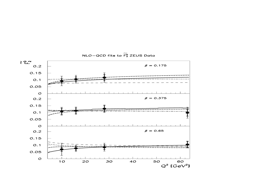
Figure 2: The $Q^{2}$ dependence of the diffractive structure function $\tilde{F}_{2}^{D}$ measured by ZEUS, together with our fits. The description of the lines and error bars is the same as in Fig. 1.

Our first fit, A, has as its initial distribution a hard quark distribution (proportional to $\beta(1-\beta)$) with no glue, and hence one adjustable parameter, whose value is the result of the fit:

$$\beta f^{A}_{q/{\mathbb{P}}}(\beta,Q_{0}^{2}) = 0.585\,\beta(1-\beta),$$

$$\beta f^{A}_{g/{\mathbb{P}}}(\beta,Q_{0}^{2}) = 0.$$ (18)

This fit gives the dashed line in the figures. It represents the shape of the diffractive structure function $\tilde{F}_{2}^{D}$ moderately well, but there are noticeable deviations, both as a function of $Q^{2}$ and of $\beta$.

For the $Q^{2}$-dependence, Fig. 2, we see that fit A results in an $\tilde{F}_{2}^{D}$ that at large $\beta$ decreases with $Q^{2}$, whereas the data show a tendency to increase. At small $\beta$, both the data and the fit rise with $Q^{2}$, but the data rise more rapidly. This suggests adding in an initial gluon distribution, whose effect is to make the quark distributions rise. As to the $\beta$-dependence, we see from Fig. 1, that the fit gives an $\tilde{F}_{2}^{D}$ that is rather higher than the data at large $\beta$ and rather lower at small $\beta$. This suggests that an admixture of soft quarks, more peaked at small $\beta$ would improve the fit noticeably.

So we try each of these additions in turn, and then together. First, in fit B we allow a hard gluon in the initial distribution, with the result:

$$\beta f^{B}_{q/{\mathbb{P}}}(\beta,Q_{0}^{2}) = 0.516\,\beta(1-\beta),$$

$$\beta f^{B}_{g/{\mathbb{P}}}(\beta,Q_{0}^{2}) = 12.28\,\beta(1-\beta).$$ (19)

Since the gluons only affect deep inelastic scattering in next-to-leading order (NLO), a very large gluon distribution is needed to produce a substantial effect on $\tilde{F}_{2}^{D}$. The resulting $Q^{2}$ evolution has a much more satisfactory shape, as can be seen from the thin solid line in Fig. 2. In addition, the strong gluon distribution has the effect of biasing the evolved quark distribution towards smaller $\beta$. Thus the shape of $\tilde{F}_{2}^{D}$ as a function of $\beta$ is also improved, Fig. 1.

Next, in fit C, represented by the dot-dashed line, we see the effect of adding a soft term to the quark distribution without allowing an initial gluon distribution. In general we expect a soft quark term, since Regge theory predicts that a quark distribution at small $\beta$ behaves approximately as $\beta f\sim 1$. We find the best fit of this kind to be:

$$\beta f^{C}_{q/{\mathbb{P}}}(\beta,Q_{0}^{2}) = 0.470\,\beta(1-\beta)+0.080\,(1-\beta)^{2},$$

$$\beta f^{C}_{g/{\mathbb{P}}}(\beta,Q_{0}^{2}) = 0.$$ (20)

The normalization of the hard quark term is reduced by about 20%, compared with fit A, and the added soft term clearly improves the shape of the $\beta$ distributions, in Fig. 1. It should be clear that at moderate and large values of $\beta$, above about 0.2, there is a dominant hard quark term. Moreover a soft term, at small $\beta$ is needed, no matter whether it is intrinsic to the quark distribution or whether it is generated dynamically, from evolution controlled by the gluon distribution. As is to be expected, the soft quark term does nothing to improve the $Q^{2}$ dependence in Fig. 2.

We next try both a soft quark term and a hard gluon term. This results in fit D (shown as the dotted line in the figures):

$$\beta f^{D}_{q/{\mathbb{P}}}(\beta,Q_{0}^{2}) = 0.512\,\beta(1-\beta)+0.005\,(1-\beta)^{2},$$

$$\beta f^{D}_{g/{\mathbb{P}}}(\beta,Q_{0}^{2}) = 11.65\,\beta(1-\beta).$$ (21)

This is indistinguishable from fit B, particularly given the errors. The important fact is that if the pomeron were quark dominated, QCD predicts that $\tilde{F}_{2}^{D}$ decreases with $Q^{2}$ at large $\beta$. The only way of undoing, or even reversing, this evolution is to have a large initial amount of glue. No extra soft quark term is required by the data.

Given the number of points and their errors, we can conclude that

• Hard quark and gluon distributions are preferred.

• The normalization of the quark distribution is reasonably well determined.

• Probably a substantial gluon distribution is preferred.

However, even the pure quark fit, A, gives a satisfactory $\chi^{2}$ — see Eq. (23) below. It should be remembered, however, that $\chi^{2}$ is not the only measure of goodness-of-fit. On the other hand, the error bars in the lowest plot in Fig. 2 indicate that reduction of the systematic errors in the measurement of $\partial\tilde{F}_{2}^{D}/\partial Q^{2}$ is urgently needed to improve the determination of the gluon distribution.

Finally, we recall that the H1 collaboration has shown fits to their data with a gluon distribution that is very peaked close to $\beta=1$. So we have tried a similar fit. The result, fit SG (shown as the thick solid line in the figures), is:

$$\beta f^{SG}_{q/{\mathbb{P}}}(\beta,Q_{0}^{2}) = 0.354\,\beta(1-\beta),$$

$$\beta f^{SG}_{g/{\mathbb{P}}}(\beta,Q_{0}^{2}) = 70.756\,\beta^{8}(1-\beta)^{0.3}.$$ (22)

The exponents in the gluon density of Eq. (22) were chosen to try and match the singular gluon parameterization derived by H1 [8]; the ZEUS data, at least at this time, are not able to determine definite values for these exponents. To avoid possible numerical problems with the evolution code we have chosen a shape for the gluon distribution that has a peak close to $\beta=1$ but that is not actually singular there.

The singular fit results in an improved $\chi^{2}$ — see Eq. (23) below — presumably because the resulting $\tilde{F}_{2}^{D}$ increases more rapidly with $Q^{2}$ at large $\beta$. Given the size of the systematic error bars in the relevant plot, the bottom one of Fig. 2, this reinforces the need for improving the systematic errors on $\partial\tilde{F}_{2}^{D}/\partial Q^{2}$.

In each of our fits, the parameters of the fit are the nonzero coefficients, with the exponents being held fixed. The parameters are determined by minimizing the $\chi^{2}$ between the theory and the data. The systematic and statistical errors have been added in quadrature, although that is not an ideal procedure. All the fits give a good $\chi^{2}$ and the fits with the large gluon are somewhat preferred, particularly the singular gluon fit:

Fit A Fit B Fit C Fit D Fit SG

$$\chi^{2}/\mbox{d.o.f}$$ 5.7/10 1.7/9 2.5/9 1.7/8 1.2/9

Statistical 18/10 3.8/9 6.0/9 3.8/8 3.1/9

(23)

The fact that the $\chi^{2}$ per degree of freedom for all these fits is much less than unity presumably indicates that the systematic errors have not been treated correctly, for example, as regards point-to-point correlations. However, even if only the statistical errors are taken into account, 4 of the 5 fits have a worryingly low $\chi^{2}$ per degree of freedom, as can be seen from the last line. There is only a few per cent probability of getting fits this good, even if the theory is exactly correct. We take this as an indication that one should look more carefully at the computation of the errors on the structure functions.

Independently of the quantification of the errors, the most important feature from our point of view is that the fits give rather stable normalizations to the quark distributions. The second important feature is that a very large gluon distribution is preferred, perhaps strongly peaked at large $\beta$. This is in agreement with the results presented by the H1 collaboration [8]. The momentum sums $\sum_{a}\int_{0}^{1}d\beta\beta f_{a/\mathbb{P}}(\beta)$ are given in the following table:

Fit A Fit B Fit C Fit D Fit SG

Quarks 0.39 0.34 0.42 0.35 0.24

Gluons 0 2.05 0 1.94 3.57

Total 0.39 2.39 0.42 2.29 3.81

(24)

Although the allowed gluon distributions cover a wide range, the overall normalization of the quarks is determined to about $\pm 10\%$, except in the case of the singular gluon fit, where the quarks are brought down by about 30%.

4 Numerical Calculations of $W$ and $Z$ Production

For the calculations in this section, the factorization scale in the parton distributions was set to $M_{VB}$. The values of the electroweak parameters which appear in the various formulae were taken from the particle data handbook [24], and we use only four flavors (u, d, s, c) in the weak mixing matrix, with the Cabibbo angle $\theta_{C}=0.2269$.

4.1 Comparison to previous calculations

Bruni and Ingelman [16] computed diffractive $W/Z$ cross sections up to ${\cal O}(\alpha_{s})$, i.e., including gluon contributions. These calculations neglected any $Q^{2}$ evolution of the parton distributions in the pomeron. At $\sqrt{s}=1800\ {\rm GeV}$, they obtained the following diffractive fractions ($R=\sigma^{\rm diff}/\sigma^{\rm incl}$): $R_{W^{+}+W^{-}}\simeq 17\%$ and $R_{Z}\simeq 15\%$ for total $W$ and $Z$ production, respectively. These rates are substantially larger than the few percent quoted in preliminary CDF results [10, 12].

As we will now explain, when one uses evolved pomeron parton densities from the above fits to data from the ZEUS experiment, one obtains substantially smaller rates than the Bruni-Ingelman ones. To understand these small rates, we first verify that we can reproduce the Bruni-Ingelman results. For these we used their unevolved hard quark distribution in the pomeron (given by their Eq. (4)), the same cut on $x_{{\mathbb{P}}}$: $x_{{\mathbb{P}}}^{\rm max}=0.1$, the EHLQ1 parton distributions in the proton and the Ingelman-Schlein (IS) flux factor:

$$f_{{\mathbb{P}}/p}^{\rm IS}(x_{{\mathbb{P}}})=\int dt{1\over 2.3x_{{\mathbb{P}}}}\biggl{(}6.38e^{8t}+0.424e^{3t}\biggr{)}.$$ (25)

Next, we evolved their pomeron parton distributions and recalculated the cross sections. Finally, to provide our best estimates of the rates, we repeated the calculations using CTEQ3M for the parton densities in the proton/antiproton and using our fits for the parton densities in the pomeron, all with proper evolution. All the inclusive cross sections were calculated using Eqs. (5) and (13). The results we obtained are summarized in Tables 1 to 3.

First, in Table 1, we show the inclusive cross section, $\sigma^{\rm incl}$, which will give the denominator for the fraction of the cross section which is diffractive. Our results are shown in the last column. These are 20% to 30% higher than those of Bruni and Ingelman (column 2). We have verified (column 3) that this increase is due to the use of the more up-to-date CTEQ3M densities in the proton instead of the EHLQ1 densities used by Bruni and Ingelman. Given the current accuracy of the diffractive data, we did not bother to make NLO calculations; generally the effect would be to increase the cross sections by some tens of percent.

	Ref.[16] LO
	EHLQ1	EHLQ1	CTEQ3M
$W^{+}+W^{-}$	14000	14332	18150
$Z$	4400	4407	5383

Table 1: Inclusive cross sections $\sigma^{W,Z\,\rm incl}$ (pb) for weak vector boson production.

The diffractive cross sections $\sigma^{W,Z\,\rm diff}$ are shown in Tables 2 and 3. In the columns labeled ‘BI’, we used the Bruni-Ingelman parton density in the pomeron and the EHLQ1 parton densities in the proton. In the other columns we used our fits for the parton densities in the pomeron together with the CTEQ3M parton distributions in the proton. First, we use the same cut $x_{{\mathbb{P}}}^{\rm max}=0.1$ that was used by Bruni and Ingelman, to produce Table 2. However, this allows $x_{\mathbb{P}}$ to be rather larger than where pomeron exchange is expected to dominate. So we also made calculations with $x_{{\mathbb{P}}}^{\rm max}=0.01$, for which the results are shown in Table 3.

In column 3 of Table 2 we show our results when we use the same unevolved parton densities as Bruni and Ingelman; we agree with their cross sections. Then we repeat the calculations but with correctly evolved parton densities in the pomeron, with the Bruni-Ingelman formula being used as the initial data for the evolution at $Q_{0}^{2}=5\,{\rm GeV}^{2}$. We see that this leads to about a 30% reduction in the cross section. The diffractive fraction obtained from the evolved BI pomeron parton distribution, using column 3 of Table 1 for $\sigma^{W,Z\,\rm incl}$, is about 14% for $W$ production, compared with the 19% that is obtained using the unevolved BI pomeron distributions. The corresponding percentages for $Z$ production are a little smaller: 12% and 17%.

Pomeron:	BI[16]	Our BI	BI	Fit A	Fit D
	unevolved	unevolved	evolved	evolved	evolved
Proton:	EHLQ1	EHLQ1	EHLQ1	CTEQ3M	CTEQ3M
$W^{+}+W^{-}$	2800	2768	2025	518	844
$Z$	760	738	520	133	204

Table 2: Diffractive cross section $\sigma^{W,Z\,\rm diff}$ (pb) for weak vector boson production, with $x_{\mathbb{P}}^{\rm max}=0.1$.

Pomeron:	BI (evolved)	Fit A (evolved)	Fit D (evolved)
Proton:	EHLQ1	CTEQ3M	CTEQ3M
$W^{+}+W^{-}$	52.3	12.8	13.9
$Z$	6.6	1.6	1.6

Table 3: Diffractive cross section $\sigma^{W,Z\,\rm diff}$ (pb) for weak vector boson production, but now with $x_{\mathbb{P}}^{\rm max}=0.01$.

In the last two columns of Tables 2 and 3 we present the results when two of our fits to ZEUS data are used. Fit A is the one with a simple hard quark distribution and no glue as the initial values, while fit D, together with fit B, has the smallest $\chi^{2}$. Although this latter fit has a very large gluon distribution which carries about seven times as much momentum as the quarks, the preference for a large amount of glue is mild—see the last two columns of (23). Furthermore, at $Q_{0}^{2}=4\,{\rm GeV}^{2}$, the initial quark distribution remains mostly unchanged whether there are zero gluons or, conversely, the gluons are unconstrained.

The cross sections resulting from fit A (in column 5 of Table 2) are about 25% of the evolved BI cross sections. The diffractive fractions obtained from this fit, using the CTEQ3M entries in Table 1, are 2.9% (2.5%) for $W\ (Z)$ production, as shown in Table 4.

In fit D, there is an enormous amount of glue initially, and this significantly affects the evolution of the quarks in the pomeron from $Q_{0}^{2}=4\,{\rm GeV}^{2}$ to the vector boson mass. The result is an increase in the cross section, as can be seen in column 6 of Table 2. This happens even though the initial quark distribution is smaller than in fit A. Even so, the cross sections are still smaller, by a factor of about 2, than the ones from evolved BI pomeron parton distributions. The rates from fit D are 4.7% (3.8%) for $W\ (Z)$ production. These rates are somewhat lower than those obtained by Kunszt and Stirling [19], who mostly used quark distributions that at large $\beta$ fall less steeply than ours.

The data [4] from which our fits were extracted used a conservative cut on the pomeron momentum, $x_{{\mathbb{P}}}^{\rm max}=0.01$. The pomeron flux factor allows for the $x_{\mathbb{P}}$ dependence, but to ensure maximum compatibility with the ZEUS data without the assumption of standard Regge behavior, the same cut should be applied to the cross sections in hadron-hadron collisions. This results in the cross sections in Table 3, which therefore represent our most accurate prediction of diffractive $W$ and $Z$ production, given only the assumption of hard scattering factorization, which of course we wish to test. Notice that with this cut the diffractive cross sections are over an order of magnitude smaller than with $x_{{\mathbb{P}}}^{\rm max}=0.1$. The percentages obtained with this cut on $x_{{\mathbb{P}}}$ for $W\ (Z)$ production are 0.07% (0.03%) and 0.08% (0.03%) for fits A and D, respectively, as shown in Table 4 The large reduction is presumably due to the fact that we are not far from an effective kinematic limit: the cut on $x_{\mathbb{P}}$ gives a maximum proton-pomeron energy of 180 GeV, and partons typically do not carry the whole of the energy of their parent hadrons.

	BI (unevolved)	Fit A	Fit D	Fit A	Fit D
	$x_{\mathbb{P}}^{\rm max}=0.1$	$x_{\mathbb{P}}^{\rm max}=0.1$	$x_{\mathbb{P}}^{\rm max}=0.1$	$x_{\mathbb{P}}^{\rm max}=0.01$	$x_{\mathbb{P}}^{\rm max}=0.01$
$W^{+}+W^{-}$	19%	2.9%	4.7%	0.07%	0.08%
$Z$	17%	2.5%	3.8%	0.03%	0.03%

Table 4: Diffractive fractions

4.2 Why are the fractions smaller than from BI?

Although the data used in our fits support a “hard” quark distribution in the pomeron, we predict that the diffractive $W$ and $Z$ cross sections are much smaller, by a factor of 3 to 5, than those predicted by Bruni and Ingelman, who also used hard quark distributions. This factor arises as an accumulation of several modest factors that all change the ratios in the same direction.

• A factor 0.8 because of the larger inclusive cross sections when one uses CTEQ3M instead of the obsolete EHLQ1 distributions in the proton.

• A factor 0.7 for the effect of the evolution of the parton densities in the pomeron.

• A factor 0.7 for the use of the Donnachie-Landshoff flux factor instead of the Ingelman-Schlein flux factor, when the momentum sum is kept fixed.

• A factor 0.5 because the data indicate that the quarks give a contribution to the momentum sum of 0.5 (with the DL normalization), instead of unity as assumed by Bruni and Ingelman.

4.3 Lepton distributions for $W$ production at the Tevatron

In this section, we present our results for $W$ production, but now with cuts on the emitted lepton $l$. Specifically, we calculate the electron’s (or positron’s) rapidity $(y)$ distribution from Eq. (9) for the diffractive process, and Eq. (12) for the inclusive one. For the parton distributions in the pomeron, we use our five fits, Eqs. (18)–(22), evolved up to the $W$ mass.

We impose cuts on the lepton that are appropriate for measurements [10] at the CDF experiment. A cut of 20 GeV was imposed on the $E_{T}$ of the emitted lepton so that the integration region for $E_{T}$ is $20\,{\rm GeV}\leq E_{T}\leq{1\over 2}M_{W}$. The parameter $x_{{\mathbb{P}}}$ was integrated over the range $M_{W}^{2}/s\leq x_{{\mathbb{P}}}\leq 0.01$.

Fig. 3 shows our results for $W^{-}$ production. The diffractive cross sections using fits B and D differ only by a few percent and are represented by solid curves which overlap, while those using fits A and C are denoted by the dashed and dot-dashed curves, respectively. These curves exhibit a strong fall-off in the region $y_{e}>-0.25$ that is a consequence of the requirement of a rapidity gap. The overlap between the two solid curves suggests that, at least for this particular process in this kinematic region, the extra soft term in fit D for the quark in Eq. (21) does not contribute much. The lower dotted curve is the inclusive cross section rescaled by $10^{-3}$.

The diffractive cross section is about 3% to 4.4% of the nondiffractive one at the leftmost-edge of the plots (at $y=-3$) depending on the fit used. The cross sections using fit B or fit D are about 45% larger than those using fits A and C at $y=-3$, with the ratio decreasing as $y$ increases. Since we only include the $q{\bar{q}}\to W$ channel in the calculations, and the quark densities are nearly the same for the five fits because of the small contribution of the soft term, this difference is mostly due to the effect of evolution. The presence of a large amount of glue in fits B and D increases the evolved quark densities relative to those in fits A and C. This tendency is even more pronounced for the SG fit (upper dotted curve), where the glue is concentrated at large $\beta$.

Figure 3: Rapidity Distribution of $e^{-}$ in $W^{-}$ production. A cut $x_{\mathbb{P}}<0.01$ was used.

The corresponding cross sections for $W^{+}$ are shown in Fig. 4. The cross sections are larger than for the $W^{-}$, because a valence up quark from the proton can be used to make a $W^{+}$, especially at large negative rapidities. In the plot, the rapidity gap exists for $y_{e^{+}}>-1.6$. As in the case of $W^{-}$ production, the diffractive cross section using fit B or D is larger than the one with fit A or C, by about 35% at $y_{e^{+}}=-4$, decreasing with $y_{e^{+}}$.

Figure 4: Rapidity Distribution of $e^{+}$ in $W^{+}$ production. A cut $x_{\mathbb{P}}<0.01$ was used.

4.4 Comparison to CDF data for $W$ production

The CDF collaboration has presented preliminary data on diffractive $W$ production from $p{\bar{p}}$ collisions at ${\sqrt{s}}=1800\,\rm{GeV}$ [10, 12]. The $W^{\prime}s$ are produced with a rapidity gap in the region $2.4<|\eta|<4.2$. They find that the fraction of diffractive to non-diffractive $W$ production is [12] $R_{W}=[1.15\pm 0.51({\it stat})\pm 0.23({\it syst})]\%$.

In Table 5 we present our diffractive fractions using Eq. (5) with $x_{\mathbb{P}}^{max}=0.017$, which we determined from the CDF plot [11] relating $\eta_{\it max}$ and $x_{\mathbb{P}}$. The fractions are about a factor of two smaller than the measured rates but are all within the experimental uncertainties. They are computed with the diffracted hadron being allowed to be either the proton or the antiproton.

	Fit A	Fit B	Fit C	Fit D
$W^{+}+W^{-}$	0.56%	0.67%	0.50%	0.66%

Table 5: Diffractive fractions using CDF cuts.

5 Diffractive Jets

In this section, we present our results for jet production. We imposed the following cuts on the jet cross sections. These represent the effect of appropriate experimental cuts [10, 14] and of cuts to improve the significance of the signal.

• We require that two jets are produced in the same half of the detector, i.e., $y_{1}y_{2}>0$, where $y_{i}$ is the rapidity of jet $i$. This eliminates the region where the jets are in opposite hemispheres, since that region is well populated by non-diffractive events but is relatively unpopulated by diffractive events, because of the rapidity gap requirement.

• Each jet is required to have a transverse energy $E_{T}$ greater than 20 GeV. This ensures that we are definitely in the perturbative region for the jets, but the cut could be relaxed.

• Each jet’s rapidity satisfies $|y|>y_{cut}\equiv 1.8$.

Next, we integrated over the rapidity of one of the jets to obtain a single jet distribution, but still subject to the above cuts on the other jet. Eqs. (2) and (11) were used for the diffractive and inclusive cross sections, respectively, with the parton distributions evolved to the scale $E_{T}$. The integration limits used for the $E_{T}$ integral were $E_{T}^{\rm min}=20\,{\rm GeV}$ and $E_{T}^{\rm max}=\sqrt{s}/(e^{-y}+e^{y})$, while the $x_{{\mathbb{P}}}$ integral was performed up to $x_{{\mathbb{P}}}=0.01$. In the following discussion, we will denote the rapidity of the final state jet by $y_{\rm jet}$ instead of $y$.

The resulting cross sections are shown in Fig. 5. There are no points in the middle part of the plot because of the rapidity cut used, as described above. The lower (upper) solid curve, which results from using fit D (fit B), is about 10 times larger than both the dashed and dot-dashed curves, in which fits A and C, respectively, were used. This reflects the sensitivity of this particular type of cross section to the gluon content of the pomeron. The lower dotted curve, which is symmetric about $y=0$, represents the inclusive cross section scaled down by a factor of $10^{-3}$.

We also show in Fig. 5 the cross section obtained when the pomeron parton density with a singular gluon is used (fit SG), the upper dotted curve. The resulting cross section is about $1.5$ to $2.5$ times larger than that obtained using fit B or D.

Figure 5: Rapidity Distribution of Jet Cross Sections.

The diffractive jet fractions are shown in Fig. 6, where $R\times 100$ is plotted as a function of $y_{\rm jet}$, with $R={d\sigma^{\rm jet,diff}/dy_{\rm jet}\over d\sigma^{\rm jet,incl}/dy_{\rm jet}}$. As in Fig. 5, the solid curves correspond to the rates when fits B and D are used, while the dashed and dot-dashed curves denote the rates for fits A and C, respectively. For the non-singular distributions, one finds that the rates $R$ are largest when fit B is used, varying from 4.5% to 2.2%. With fit D, which differs from fit B by the absence of a soft term in the quark distribution, the rates are about tenths of a percent lower. The rates obtained with fits A and C are almost identical and range from 0.43% to about 0.18%. The rates are largest at $y_{\rm jet}=-4$ then decrease as $y_{\rm jet}$ increases. Of course, the large rates for the distributions B and D, both with the large glue, directly result from the fact that there is a gluon induced subprocess. For comparison, we also show the even higher rates obtained using the singular gluon fit SG (dotted curve), which vary from 6.7% to 5.2%.

Figure 6: Diffractive Jet Production Rates.

We end this section by making comparisons with preliminary data on diffractive dijet production from CDF and D0 at ${\sqrt{s}}=1800\,{\rm GeV}$. CDF has measured dijet data both with a rapidity gap requirement [10] and with Roman pots [11] along the antiproton beam direction. In the first case, the cross section for dijets produced opposite a rapidity $(\eta)$ gap in the region $2.4<|\eta|<4.2$ is measured. Each jet is required to have a minimum $E_{T}$ of 20 GeV and rapidity $|\eta|>1.8$. They also measure the dijet cross section without a rapidity gap, i.e., what we refer to in this paper as the inclusive cross section. The diffractive fraction they measure is [12] $R_{JJ}=[0.62\pm 0.04\pm 0.09]\%$. The fractions that we obtain using the above cuts are shown in Table 6. The rates obtained with fit D or B are about nine times larger while those obtained with fit C or A are about 25% smaller than the measured value. Our calculation assumes that either the antiproton or the proton is diffracted.

	Fit A	Fit B	Fit C	Fit D
${\sigma^{\rm jet,diff}\over\sigma^{\rm jet,incl}}$	0.47%	5.6%	0.47%	5.4%

Table 6: Diffractive fractions for dijet production using CDF cuts (rapidity gap).

With their Roman pot triggered diffractive sample, CDF has measured a diffractive fraction of $R_{JJ}=[0.109\pm 0.003\pm 0.016]\%$. The data in this sample correspond to $x_{\mathbb{P}}$ in the range $0.05<x_{\mathbb{P}}<0.1$, with the jets having minimum $E_{T}$ of 10 GeV. The fractions we obtain using the same kinematic cuts are presented in Table 7. The ones obtained with fits D, B are an order of magnitude larger than the data, while those obtained with fits C, A are about 3–4 times larger. Our calculation assumes that only the antiproton is diffracted. Since our diffractive parton densities are fitted to data in which the proton may be excited, our predictions should be reduced by about $(15\pm 10)\%$ [4] before being compared with data in which the isolated proton is detected. However, even after this reduction, our predictions are still well above the measured diffractive fraction.

	Fit A	Fit B	Fit C	Fit D
${\sigma^{\rm jet,diff}\over\sigma^{\rm jet,incl}}$	0.33%	4.45%	0.37%	4.24%

Table 7: Diffractive fractions for dijet production using CDF cuts (Roman pots).

Finally, D0 also has some preliminary data [14] on diffractive dijet production. They require a rapidity gap opposite the dijets which have $E_{T}^{min}=12\,{\rm GeV}$ and $|\eta_{jet}|>1.6$. The diffractive fraction they measure is $R_{JJ}=[0.67\pm 0.05]\%$. Our calculated fractions are shown in Table 8. Again, the fractions obtained using fits D, B are an order of magnitude larger than the data, while those obtained with fits C, A are consistent with the data. Our calculation assumes that either the antiproton or the proton is diffracted.

	Fit A	Fit B	Fit C	Fit D
${\sigma^{\rm jet,diff}\over\sigma^{\rm jet,incl}}$	0.8%	10.4%	0.9%	10.0%

Table 8: Diffractive fractions for dijet production using D0 cuts (rapidity gap).

6 Conclusions

We have presented fits to the DIS diffractive structure functions measured by the ZEUS collaboration, together with a lowest order calculation of the resulting diffractive cross sections for vector boson production and jet production from $p{\bar{p}}$ interactions at the Tevatron. Since we used pomeron parton distributions fitted to data on diffractive DIS, the rates represent a realistic prediction of the cross sections, given the assumption of factorization.

The quark distributions are fairly well determined, at least in overall size, and we see that diffractive $W$ and $Z$ production is predicted to be a few percent of the inclusive cross section, at least if suitable cuts are made to select kinematic configurations that are preferentially populated in diffractive events.

We have derived fractional rates $R=\sigma^{\rm diff}/\sigma^{\rm incl}$ which are much smaller than those obtained in the benchmark studies [16] of vector boson production. The rates we have calculated are 0.08% (0.03%) for $W\ (Z)$ production using fit D, and a cut $x_{\mathbb{P}}<0.01$. For the case of lepton decays of vector bosons, we are able to increase these fractions to several percent by requiring the lepton to have large rapidity, on the side opposite the rapidity gap. Substantial deviations from these rates would indicate a breakdown of hard scattering factorization for diffractive processes. In fact, the preliminary data from the Tevatron appear to be consistent with our calculations, within large errors.

The wide range of gluon distributions that is permitted by the DIS data yields predictions for the diffractive jet cross section at the Tevatron (see Fig. 5) which differ by an order of magnitude. Given the assumption of factorization, the smaller jet cross sections, from fits A and C, represent the lowest reasonable cross sections since they correspond to a pomeron without glue at $Q_{0}^{2}=4\,{\rm GeV}^{2}$. However, the fits with the large gluon initial distributions (fits B, D, and SG) are preferred for the ZEUS DIS data, in agreement with the results [8] from the H1 collaboration.

For jet production, rates of 4.5% to 2.1% in the rapidity range $-4<y_{\rm jet}<-1.8$ were calculated using fit D or B (with the large glue). The corresponding rates for the calculations using fit A or C (with the small gluon distribution), in the same rapidity range, vary from 0.43% to 0.18%. We are working on using data [9] on diffractive photoproduction of jets to reduce greatly the uncertainty in the gluon density. This will improve the accuracy of our predictions, particularly for diffractive jet production. We can already see from the results reported by the ZEUS collaboration [9] that parton distributions with a substantial amount of glue are preferred.

As we saw at the end of Sect. 5, only the lowest of the jet cross sections we compute for the Tevatron is consistent with the data. These are the cross sections for which there is no initial glue in the parton densities. In the case of the Roman pot data, our calculated cross sections are all well above the experimental value; these are the data for which the cuts can be most directly implemented in our calculations. These results combined with the ZEUS measurement of a substantial gluon component in the pomeron already are suggestive of a breakdown of factorization.

With a modest increase in accuracy, comparison with actual data for diffractive $W$, $Z$ and jet cross sections will permit a good test of the factorization hypothesis. As explained in Ref. [1], the results of such a test will be important as a probe of the space-time structure of hadron-hadron scattering at high energy.

References

- [1] J.C. Collins, L. Frankfurt and M. Strikman, Phys. Lett. B307, 161 (1993); A. Berera and J.C. Collins, Nucl. Phys. B474, 183 (1996).
- [2] G. Ingelman and P.E. Schlein, Phys. Lett. B152, 256 (1985).
- [3] J.C. Collins, J. Huston, J. Pumplin, H. Weerts and J.J. Whitmore, Phys. Rev. D51, 3182 (1995).
- [4] ZEUS Collaboration, M. Derrick et al, Z. Phys. C68, 569 (1995).
-
[5]
ZEUS Collaboration, M. Derrick et al,
Phys. Lett. B315, 481 (1993); B332, 228 (1994);
H1 Collaboration, T. Ahmed et al, Nucl. Phys. B429, 477 (1994). - [6] UA8 Collaboration, A. Brandt et al., Phys. Lett. B297, 417 (1992).
- [7] K. Eggert, UA1 Collaboration, “Search for diffractive heavy flavour production at the CERN proton-antiproton collider” in “Elastic and Diffractive Scattering” (K. Goulianos, ed.) (Editions Frontières, Gif-sur-Yvette, 1988).
-
[8]
H1 Collaboration, “A Measurement and QCD Analysis of the Diffractive
Structure Function ”, submitted to ICHEP’96, H1 preprint
pa02-061, obtainable electronically at
http://dice2.desy.de/h1/www/psfiles/confpap/warsaw96/list.html. - [9] ZEUS Collaboration, M. Derrick et al, Phys. Lett. B356, 129 (1995).
- [10] K. Goulianos, for CDF Collaboration, “New Evidence for Rapidity Gaps Between Jets and Diffractive and Dijet Production at CDF”, Fermilab-Conf-96/233-E.
- [11] P.L. Mélèse, for CDF Collaboration, “Diffractive Dijet Search with Roman Pots at CDF”, Fermilab-Conf-96/231-E.
- [12] S. Bagdasarov, talk given at 3rd Workshop on Small and Diffractive Physics, 26–29 Sept. 1996, Argonne, IL.
- [13] K. Mauritz, for D0 Collaboration, “Hard Diffraction at D0”, talk presented at Small meeting, Sept. 28, 1996, Argonne, IL.
- [14] S. Abachi, for D0 Collaboration, “Hard Single Diffractive Jet Production at D0”, Fermilab-Conf-96/247-E.
- [15] A.G. Brandt, for D0 Collaboration, “Rapidity Gaps in Jet Events at D0”, Fermilab-Conf-96/185-E.
- [16] P. Bruni and G. Ingelman, Phys. Lett. B311, 317 (1993).
- [17] K. Goulianos, “Renormalized diffractive cross-sections at HERA and the structure of the pomeron”, Talk given at 7th Rencontres de Blois: Frontiers in Strong Interactions - 6th International Conference on Elastic and Diffractive Scattering, Blois, France, 20–24 June 1995, e-Print Archive: hep-ph/9512291
- [18] T. Gehrmann and W.J. Stirling, Z. Phys. C70, 89 (1996).
- [19] Z. Kunszt and W.J. Stirling, “Hard diffractive scattering: partons and QCD”, e-print archive hep-ph/9609245.
- [20] K Golec-Biernat and J. Kwieciński, Phys. Lett. B353, 329 (1995).
- [21] A. Donnachie and P.V. Landshoff, Phys. Lett. B191, 309 (1987); Nucl. Phys. B303, 634 (1988).
- [22] E. Eichten, I. Hinchliffe, K. Lane and C. Quigg, Rev. Mod. Phys. 56, 579 (1984); 58, 1065 (1986).
-
[23]
The CTEQ evolution package can be obtained from
http://www.phys.psu.edu/~cteq/. - [24] Particle Data Group, Phys. Rev. D54, 1 (1996).