Effects of Non-Standard Tri-linear Couplings in Photon-Photon Collisions: I. $\gamma\gamma\rightarrow W^{+}W^{-}\;$

M. Baillargeon1, G. Bélanger2 and F. Boudjema2

1. Grupo Teórico de Altas Energias, Instituto Superior Técnico

Edifício Ciência (Física) P-1096 Lisboa Codex, Portugal

2. Laboratoire de Physique Théorique ENSLAPP

Chemin de Bellevue, B.P. 110, F-74941 Annecy-le-Vieux, Cedex, France.

Abstract

The effect of anomalous couplings in $\gamma\gamma\rightarrow W^{+}W^{-}$ is studied for different energies of the $\gamma\gamma$ mode of the next linear collider. The analysis based on the maximum likelihood method exploits the variables in the four-fermion semi-leptonic final state. Polarised differential cross sections based on the complete set of diagrams for these channels with the inclusion of anomalous couplings are used and compared to an approximation based on $\gamma\gamma\rightarrow W^{+}W^{-}$ with full spin correlations. To critically compare these results with those obtained in $e^{+}e^{-}$ we perform an analysis based on the complete calculation of the four-fermion semi-leptonic final state. The anomalous couplings that we consider are derived from the next-to-leading order operators in the non-linear realisation of symmetry breaking.

ENSLAPP-A-636/97

FISIST/3-97/CFIF

Jan. 1997

1 Introduction

The next linear $e^{+}e^{-}\;$collider[1] can be turned into a $\gamma\gamma$ collider[2] by converting the single pass electrons into very energetic photons through Compton backscattering of a laser light, whereby the obtained photon can take as much as $80\%$ of the initial beam energy. The main attractions of such a mode of the next linear collider rest on its ability to study in detail the properties of a Higgs [3, 4, 5, 6] that can be produced as a resonance, since two photons can be in a $J_{Z}=0$ state whereas chirality very much suppresses this configuration with the $e^{+}e^{-}\;$pair. Also, because cross sections for the production of weak vector bosons are much larger in the $\gamma\gamma$ mode than in $e^{+}e^{-}\;$[7], the very large samples of $W$’s could allow for high precision measurements on the properties of these gauge bosons. Considering that the physics of $W$’s could reveal much on the dynamics of the Goldstone bosons through the longitudinal component of the $W$’s this mode of the linear collider may appear ideal for an investigation of the mechanism of symmetry breaking.
However, it is also true that these important issues can be easily blurred by backgrounds that are often quite large in the photon mode. For instance, in the case of the Higgs, a resonant signal is viable only for a light Higgs after judiciously tuning the parameters (energies and polarisations) of the $\gamma\gamma$ collider[8, 9, 10]. The aim of the present paper is to critically analyse the extent to which the reaction $\gamma\gamma\rightarrow W^{+}W^{-}\;$can be useful in measuring the electromagnetic couplings of the $W$ and how these measurements compare to those one could perform in the “natural” $e^{+}e^{-}\;$mode of the next collider. From the outset, one would naively expect the $\gamma\gamma$ mode to fare much better than the $e^{+}e^{-}\;$mode when it comes to the anomalous $WW\gamma$ couplings, not only because the $WW$ statistics is much larger in the photon mode but also because the most promising reaction in $e^{+}e^{-}\;$, $e^{+}e^{-}\rightarrow W^{+}W^{-}\;$, accesses not only $WW\gamma$ but also the $WWZ$ couplings. If these two types of couplings were not related to each other, as one has generally assumed, then it is quite difficult to disentangle a $WW\gamma$ and a $WWZ$ coupling at the $e^{+}e^{-}\;$mode, whereas obviously only the former can be probed at the $\gamma\gamma$ mode. However, as we will argue, the electroweak precision measurements at the $Z$ peak are a sign that there should be a hierarchy of couplings whereby the symmetries one has observed at the present energies indicate that the $WW\gamma$ and the $WWZ$ should be related. If this is so, though $\gamma\gamma\rightarrow W^{+}W^{-}\;$is unique in unambiguously measuring the $WW\gamma$ couplings, it is somehow probing the same parameter space as $e^{+}e^{-}\rightarrow W^{+}W^{-}\;$. In such an eventuality one should then enquire about how to exploit the $\gamma\gamma$ mode, and whether the reaction $\gamma\gamma\rightarrow W^{+}W^{-}\;$can give more stringent constraints than in the $e^{+}e^{-}\;$mode. In addition it is useful to investigate whether one may gain by combining the results of the $\gamma\gamma$ analysis with those obtained in the $e^{+}e^{-}\;$mode. These two aspects will be addressed in the present paper.

Although there have been numerous studies that dealt with the subject of the tri-linear anomalous couplings in $\gamma\gamma\rightarrow W^{+}W^{-}\;$[11], they have all been conducted at the level of the $\gamma\gamma\rightarrow W^{+}W^{-}\;$cross section. As we will show, even if one assumes reconstruction of the helicities of the $W$, restricting the analysis of the $\gamma\gamma\rightarrow W^{+}W^{-}\;$at the level of the cross section, where one only accesses the diagonal elements of the $WW$ density matrix, it is not possible to maximally enhance the effect of the anomalous couplings. Indeed, as one expects in an investigation of the Goldtsone sector, the new physics parameterised in this context by an anomalous magnetic moment of the $W$, $\Delta\kappa_{\gamma}$, affects principally the production of two longitudinal $W$ bosons. In the $\gamma\gamma$ mode this affects predominantly the $J_{Z}=0$ amplitude by providing an enhanced coupling of the order $\gamma=s_{\gamma\gamma}/{M_{W}^{2}}$ ($\sqrt{s_{\gamma\gamma}}$ is the $\gamma\gamma$ centre of mass energy). Unfortunately the same standard amplitude (the $J_{Z}=0$ with two longitudinal W’s) has the factor $1/\gamma$ and therefore the interference is not effective in the sense that the genuine enhanced coupling $\gamma$ brought about by the new physics is washed out. This is in contrast with what happens in the $e^{+}e^{-}\;$mode where the interference is fully effective. Nonetheless, the enhanced coupling could still be exploited in the $\gamma\gamma$ mode if one is able to reconstruct the non diagonal elements of the $WW$ density matrix. This can be done by analysing the distributions involving kinematical variables of the decay products of the $W$. In any case, in a realistic set-up the $W$’s are only reconstructed from their decay products and since we would need to impose cuts on the fermions, one absolutely requires to have at hand the distributions of the fermions emerging from the $W$’s. One thus needs the fully polarised $WW$ density matrix elements which one combines with the polarised decay functions in order to keep the full spin correlations and arrive at a more precise description of $\gamma\gamma\rightarrow W^{+}W^{-}\;$in terms of $\gamma\gamma\rightarrow W^{+}W^{-}\rightarrow 4f$. Having access to all the kinematics of the fermionic final states, one can exploit the powerful technique of the maximum likelihood method, ML, to search for an anomalous behaviour that can affect any of the distributions of the 4-fermion final state and in our case unravel the contribution of the non-diagonal elements of the $WW$ density matrix which are most sensitive to the anomalous couplings. The exploitation of the density matrix elements in $e^{+}e^{-}\rightarrow W^{+}W^{-}\;$has been found to be a powerful tool not only at LEP2 energies [12, 13, 14] but also at the next collider[15, 16, 17, 18], however a thorough investigation in $\gamma\gamma$ is missing.
In a previous paper[19], dedicated to four fermion final states in $\gamma\gamma$ within the ${\cal{S}}{\cal{M}}\;$, we have shown that these signatures could be very well approximated by taking into account only the $WW$ resonant diagrams provided these were computed through the density matrix formalism and a smearing factor taking into account the finite width of the $W$ is applied. In this paper we will not only consider the fully correlated $WW$ cross sections leading to a semi-leptonic final state taking into account the anomalous couplings but we will also consider the full set of the four-fermion final states including those anomalous couplings, thus avoiding any possible bias. Having extracted the limits on the anomalous couplings in $\gamma\gamma$ we will contrast them with those one obtains in $e^{+}e^{-}\;$. For the latter we conduct our own analysis based on the same set of parameters as in the $\gamma\gamma$ mode and most importantly taking into account the full set of four fermion diagrams. The maximum likelihood method is used throughout.
The anomalous couplings that we study in this paper are derived from a chiral Lagrangian formulation which does not require the Higgs[20]. To critically compare the performance of the $e^{+}e^{-}\;$and the $\gamma\gamma$ mode, we will first consider the case where a full SU(2) global symmetry is implemented as well as a situation where one allows a breaking of this symmetry. We will see that the advantages of the $\gamma\gamma$ mode depend crucially on the model considered.
Our paper is organised as follows. After a brief motivation of the chiral Lagrangian and a presentation of the operators that we want to probe, we give in section 3 a full description of the helicity amplitudes and of the density matrix for $\gamma\gamma\rightarrow W^{+}W^{-}\;$including the anomalous couplings. We then proceed to extract limits on the couplings by exploiting the maximum likelihood method both for the “resonant” diagrams as well as for the complete set of Feynman diagrams for the 4-fermion final state, for various combinations of the photon helicities. We then discuss the limits one obtains in $e^{+}e^{-}\;$and compare them with those one obtains in $\gamma\gamma$ for different centre-of-mass energies. The last section contains our conclusions.

2 Anomalous couplings and the chiral Lagrangian

If by the time the next linear collider is built and if after a short run there has been no sign of a Higgs, one would have learnt that the supersymmetric extension of the ${\cal{S}}{\cal{M}}\;$may not be realised, at least in its simplest form, and that the weak vector bosons may become strongly interacting. In this scenario, in order to probe the mechanism of symmetry breaking it will be of utmost importance to scrutinise the dynamics of the weak vector bosons since their longitudinal modes stem from the Goldstones bosons which are the remnants of the symmetry breaking sector. Well before the opening up of new thresholds one expects the dynamics of the symmetry breaking sector to affect the self-couplings of the gauge bosons. The natural framework to describe, in a most general way, the physics that make do with a Higgs and that parameterises these self-couplings relies on an effective Lagrangian adapted from pion physics where the symmetry breaking is non-linearly realised [20]. This effective Lagrangian incorporates all the symmetries which have been verified so far, especially the gauge symmetry. We will assume that the gauge symmetry is $SU(2)\times U(1)\,$. Moreover present precision measurements indicate that the $\rho$ parameter is such that $\rho\sim 1$ [21]. This suggests that the electroweak interaction has a custodial global SU(2) symmetry (after switching off the gauge couplings), whose slight breaking seems to be entirely due to the bottom-top mass splitting. This additional symmetry may be imposed on the effective Lagrangian. We will also assume that ${\cal{C}}{\cal{P}}\;$is an exact symmetry. These ingredients should be incorporated when constructing the effective Lagrangian. The construction and approach has, lately, become widespread in discussing weak bosons anomalous couplings in the absence of a Higgs.
The effective Lagrangian is organised as a set of operators whose leading order operators (in an energy expansion) reproduce the “Higgsless” standard model. Introducing our notations, as concerns the purely bosonic sector, the SU(2) kinetic term that gives the standard tree-level gauge self-couplings is

$${{\cal L}}_{{\rm Gauge}}=-\frac{1}{2}\left[{\rm Tr}({\mbox{\boldmath$W$}}_{\mu\nu}{\mbox{\boldmath$W$}}^{\mu\nu})+{\rm Tr}({\mbox{\boldmath$B$}}_{\mu\nu}{\mbox{\boldmath$B$}}^{\mu\nu})\right]$$ (2.1)

where the $SU(2)$ gauge fields are ${\mbox{\boldmath$W$}}_{\mu}=W^{i}_{\mu}\tau^{i}$, while the hypercharge field is denoted by ${\mbox{\boldmath$B$}}_{\mu}=\tau_{3}B_{\mu}$. The normalisation for the Pauli matrices is ${\rm Tr}(\tau^{i}\tau^{j})=2\delta^{ij}$. We define the field strength as, ${\mbox{\boldmath$W$}}_{\mu\nu}$

$${\mbox{\boldmath$W$}}_{\mu\nu} = \frac{1}{2}\left(\partial_{\mu}{\mbox{\boldmath$W$}}_{\nu}-\partial_{\nu}{\mbox{\boldmath$W$}}_{\mu}+\frac{i}{2}g[{\mbox{\boldmath$W$}}_{\mu},{\mbox{\boldmath$W$}}_{\nu}]\right)$$ (2.2)

$$= \frac{\tau^{i}}{2}\left(\partial_{\mu}W^{i}_{\nu}-\partial_{\nu}W^{i}_{\mu}-g\epsilon^{ijk}W_{\mu}^{j}W_{\nu}^{k}\right)$$

The Goldstone bosons, $\omega^{i}$, within the built-in SU(2) symmetry are assembled in a matrix $\Sigma$

$$\Sigma=exp(\frac{i\omega^{i}\tau^{i}}{v})\;\;;v=246~{}GeV\;\;\;\mbox{ and}\;\;{{\cal D}}_{\mu}\Sigma=\partial_{\mu}\Sigma+\frac{i}{2}\left(g{\mbox{\boldmath$W$}}_{\mu}\Sigma-g^{\prime}B_{\mu}\Sigma\tau_{3}\right)$$ (2.3)

This leads to the gauge invariant mass term for the $W$ and $Z$

$${{\cal L}}_{M}=\frac{v^{2}}{4}{\rm Tr}({{\cal D}}^{\mu}\Sigma^{\dagger}{{\cal D}}_{\mu}\Sigma)\equiv-\frac{v^{2}}{4}{\rm Tr}\left({{\cal V}}_{\mu}{{\cal V}}^{\mu}\right)\;\;\;\;\;\;{{\cal V}}_{\mu}=\left({{\cal D}}_{\mu}\Sigma\right)\Sigma^{\dagger}\;\;;\;\;M_{W}=\frac{gv}{2}$$ (2.4)

The above operators are the leading order operators in conformity with the $SU(2)\times U(1)\,$gauge symmetry and which incorporate the custodial SU(2) symmetry. They thus represent the minimal Higgsless electroweak model. At the same order we may include a breaking of the global symmetry through

$${{\cal L}}_{\Delta\rho}=\Delta\rho\frac{v^{2}}{8}\left({\rm Tr}({{\cal V}}_{\mu}X)\right)^{2}\;\;\;;\;\;\;X=\Sigma\tau^{3}\Sigma^{\dagger}$$ (2.5)

Global fits from the present data give[21], after having subtracted the ${\cal{S}}{\cal{M}}\;$contributions

$$-.1\;<\;10^{3}\;\Delta\rho_{New}\;<\;2.5$$ (2.6)

Different scenarios of New Physics connected with symmetry breaking are described by the Next-to-Leading-Order (NLO) operators. Maintaining the custodial symmetry only a few operators are possible

$${{\cal L}}_{NLO}= + gg^{\prime}\frac{L_{10}}{16\pi^{2}}{\rm Tr}(\Sigma{\mbox{\boldmath$B$}}^{\mu\nu}\Sigma^{\dagger}{\mbox{\boldmath$W$}}_{\mu\nu})$$ (2.7)

$$- ig^{\prime}\frac{L_{9R}}{16\pi^{2}}{\rm Tr}({\bf B}^{\mu\nu}{{\cal D}}_{\mu}\Sigma^{\dagger}{{\cal D}}_{\nu}\Sigma)-ig\frac{L_{9L}}{16\pi^{2}}{\rm Tr}({\mbox{\boldmath$W$}}^{\mu\nu}{{\cal D}}_{\mu}\Sigma{{\cal D}}_{\nu}\Sigma^{\dagger})$$

$$+ \frac{L_{1}}{16\pi^{2}}\left({\rm Tr}(D^{\mu}\Sigma^{\dagger}D_{\mu}\Sigma)\right)^{2}+\frac{L_{2}}{16\pi^{2}}\left({\rm Tr}(D^{\mu}\Sigma^{\dagger}D_{\nu}\Sigma)\right)^{2}$$

Some important remarks are in order. Although these are New Physics operators that should exhibit the corresponding new scale $\Lambda$, such a scale does not appear in our definitions. Implicitly, one has in Eq. 2.7 $\Lambda=4\pi v\simeq 3.1TeV$. The first operator $L_{10}$ contributes directly at tree-level to the two-point functions. The latter are extremely well measured at LEP1/SLC. Indeed $L_{10}$ is directly related to the new physics contribution to the Peskin-Takeuchi parameter[22], $S_{{\rm new}}$: $L_{10}=-\pi S_{{\rm new}}$. The present inferred value of $L_{10}$ is $-1.2\leq L_{10}\leq 0.1$[21], after allowing for the ${\cal{S}}{\cal{M}}\;$contribution. We will hardly improve on this limit in future experiments through double pair production, like $e^{+}e^{-}\rightarrow W^{+}W^{-}\;$and $\gamma\gamma\rightarrow W^{+}W^{-}\;$. Therefore in the rest of the analysis we will set $L_{10}=0$ and enquire whether one can set constraints of this order on the remaining parameters. If so, this will put extremely powerful constraints on the building of possible models of symmetry breaking. The two last operators, $L_{1}$ and $L_{2}$ are the only ones that remain upon switching off the gauge couplings. They give rise to genuine quartic couplings that involve four predominantly longitudinal states. Therefore, phenomenologically, these would be the most likely to give large effects. Unfortunately they do not contribute to $\gamma\gamma\rightarrow W^{+}W^{-}\;$nor to $e^{+}e^{-}\rightarrow W^{+}W^{-}\;$. Within the constraint of SU(2) global symmetry one is left with only the two operators $L_{9L,9R}$.

Both $L_{9L}$ and $L_{9R}$ induce ${\cal{C}}\;$and ${\cal{P}}\;$conserving $\gamma WW$ and $ZWW$ couplings. In fact, for $WW\gamma$ both operators contribute equally to the same Lorentz structure and thus there is no way that $\gamma\gamma\rightarrow W^{+}W^{-}\;$could differentiate between these two operators.
By allowing for custodial symmetry breaking terms more operators are possible. A “naturality argument” would suggest that the coefficients of these operators should be suppressed by a factor $\Delta\rho$ compared to those of $L_{9}$, following the observed hierarchy in the leading order operators. One of these operators([25],[26]) stands out, because it leads to ${\cal{C}}\;$and ${\cal{P}}\;$violation and only affects the $WWZ$ vertex, and hence only contributes to $e^{+}e^{-}\rightarrow W^{+}W^{-}\;$:

$${{\cal L}}\kern-6.00006pt{/}_{c}\kern-3.99994pt{/}=g\frac{L_{c}}{16\pi^{2}}\left({\rm Tr}(\widetilde{{\mbox{\boldmath$W$}}}^{\mu\nu}{{\cal V}}_{\mu})\right)\left({\rm Tr}(X{{\cal V}}_{\nu})\right)\;\;\;;\;\;\widetilde{{\mbox{\boldmath$W$}}}^{\mu\nu}=\frac{1}{2}\epsilon^{\mu\nu\alpha\beta}\;{\mbox{\boldmath$W$}}_{\alpha\beta}$$ (2.8)

For completeness we will also consider another operator which breaks this global symmetry without leading to any ${\cal{C}}\;$and ${\cal{P}}\;$breaking:

$${{\cal L}}\kern-6.00006pt{/}_{1}=ig\frac{L\kern-4.49997pt{/}_{1}}{16\pi^{2}}\left({\rm Tr}({\mbox{\boldmath$W$}}^{\mu\nu}X)\right)\left({\rm Tr}(X[{{\cal V}}_{\mu},{{\cal V}}_{\nu}])\right)$$ (2.9)

It has become customary to refer to the popular phenomenological parametrisation (the HPZH parameterization)[27] that gives the most general tri-linear coupling that could contribute to $e^{+}e^{-}\rightarrow W^{+}W^{-}\;$. We reproduce it here to show how the above chiral Lagrangian operators show up in $e^{+}e^{-}\rightarrow W^{+}W^{-}\;$and $\gamma\gamma\rightarrow W^{+}W^{-}\;$. The phenomenological parametrisation writes

$${\cal L}_{WWV} = -ie\left\{\left[A_{\mu}\left(W^{-\mu\nu}W^{+}_{\nu}-W^{+\mu\nu}W^{-}_{\nu}\right)+\overbrace{(1+\mbox{\boldmath$\Delta\kappa_{\gamma}$})}^{\kappa_{\gamma}}F_{\mu\nu}W^{+\mu}W^{-\nu}\right]\right.$$

$$+\left.cotg\theta_{w}\left[\overbrace{(1+{\bf\Delta g_{1}^{Z}})}^{g_{1}^{Z}}Z_{\mu}\left(W^{-\mu\nu}W^{+}_{\nu}-W^{+\mu\nu}W^{-}_{\nu}\right)+\overbrace{(1+\mbox{\boldmath$\Delta\kappa_{Z}$})}^{\kappa_{Z}}Z_{\mu\nu}W^{+\mu}W^{-\nu}\right]\right.$$

$$+\left.\frac{1}{M_{W}^{2}}\left(\mbox{\boldmath$\lambda_{\gamma}$}\;F^{\nu\lambda}+\mbox{\boldmath$\lambda_{Z}$}\;cotg\theta_{w}Z^{\nu\lambda}\right)W^{+}_{\lambda\mu}W^{-\mu}_{\;\;\;\;\;\nu}\right\}$$

$$- e\frac{c_{W}}{s_{W}}g_{5}^{Z}\left\{\epsilon^{\mu\nu\rho\sigma}\left(W_{\mu}^{+}(\partial_{\rho}W_{\nu})-(\partial_{\rho}W_{\mu}^{+})W_{\nu}\right)Z_{\sigma}\right\}$$

To map the operators we have introduced into this parameterisation one needs to specialise to the unitary gauge by setting the Goldstone ($\omega_{i}$) fields to zero ($\Sigma\rightarrow 1$). We find

$$\Delta\kappa_{\gamma} = \frac{e^{2}}{s_{w}^{2}}\frac{1}{32\pi^{2}}\left(L_{9L}+L_{9R}+4L\kern-4.49997pt{/}_{1}\right)\equiv\frac{e^{2}}{s_{w}^{2}}\frac{1}{32\pi^{2}}L_{\gamma}$$

$$\Delta\kappa_{Z} = \frac{e^{2}}{s_{w}^{2}}\frac{1}{32\pi^{2}}\left(L_{9L}-\frac{s_{w}^{2}}{c_{w}^{2}}L_{9R}+4L\kern-4.49997pt{/}_{1}\right)$$

$$\Delta g_{1}^{Z} = \frac{e^{2}}{s_{w}^{2}}\frac{1}{32\pi^{2}}\left(\frac{L_{9L}}{c_{w}^{2}}\right)$$

$$g_{5}^{Z} = \frac{e^{2}}{32\pi^{2}\sin^{2}\theta_{w}}\left(-\frac{L_{c}}{\cos^{2}\theta_{w}}\right)$$

$$\lambda_{\gamma} = \lambda_{Z}=0$$ (2.11)

It is important to note that within the Higgless implementation of the “anomalous” couplings the $\lambda_{\gamma,Z}$ are not induced at the next-to-leading order. They represent weak bosons that are essentially transverse and therefore do not efficiently probe the symmetry breaking sector as evidenced by the fact that they do not involve the Goldstone bosons. It is worth remarking that, in effect, within the chiral Lagrangian approach there is essentially only one effective coupling parameterised by $\Delta\kappa_{\gamma}$ that one may reach in $\gamma\gamma$ . Thus $\gamma\gamma\rightarrow W^{+}W^{-}\;$probes the collective combination $L_{\gamma}\equiv L_{9L}+L_{9R}+4L\kern-4.49997pt{/}_{1}$. However the four independent operators contribute differently to the various Lorentz structure of $WWZ$ and thus to $e^{+}e^{-}\rightarrow W^{+}W^{-}\;$.

For completeness here are the quartic couplings that accompany the tri-linear parts as derived from the chiral effective Lagrangian

$${{\cal L}}^{SM}_{WWV_{1}V_{2}} = -e^{2}\left\{\left(A_{\mu}A^{\mu}W^{+}_{\nu}W^{-\nu}-A^{\mu}A^{\nu}W^{+}_{\mu}W^{-}_{\nu}\right)\right.$$

$$+ 2\frac{c_{w}}{s_{w}}(1+\frac{l_{9l}}{c_{w}^{2}})\left(A_{\mu}Z^{\mu}W^{+}_{\nu}W^{-\nu}-\frac{1}{2}A^{\mu}Z^{\nu}(W^{+}_{\mu}W^{-}_{\nu}+W^{+}_{\nu}W^{-}_{\mu})\right)$$

$$+ \frac{c_{w}^{2}}{s_{w}^{2}}(1+\frac{2l_{9l}}{c_{w}^{2}}-\frac{l_{-}}{c_{w}^{4}})\left(Z_{\mu}Z^{\mu}W^{+}_{\nu}W^{-\nu}-Z^{\mu}Z^{\nu}W^{+}_{\mu}W^{-}_{\nu}\right)$$

$$+ \frac{1}{2s_{w}^{2}}(1+2l_{9l}-l_{-})\left(W^{+\mu}W^{-}_{\mu}W^{+\nu}W^{-}_{\nu}-W^{+\mu}W^{+}_{\mu}W^{-\nu}W^{-}_{\nu}\right)$$

$$- \frac{l_{+}}{2s_{w}^{2}}\left(\left(3W^{+\mu}W^{-}_{\mu}W^{+\nu}W^{-}_{\nu}+W^{+\mu}W^{+}_{\mu}W^{-\nu}W^{-}_{\nu}\right)\right.$$

$$+ \frac{2}{c_{w}^{2}}\left.\left.\left(Z_{\mu}Z^{\mu}W^{+}_{\nu}W^{-\nu}+Z^{\mu}Z^{\nu}W^{+}_{\mu}W^{-}_{\nu}\right)+\frac{1}{c_{w}^{4}}Z_{\mu}Z^{\mu}Z_{\nu}Z^{\nu}\right)\right.$$

$$- \left.2i\frac{c_{W}}{s_{W}}g_{5}^{Z}\varepsilon^{\mu\nu\alpha\beta}A^{\mu}Z^{\nu}W^{+}_{\alpha}W^{-}_{\beta}\right\}$$

$${\rm with} (l_{9l},r_{9},\tilde{l}_{1})=\frac{e^{2}}{32\pi^{2}s_{w}^{2}}(L_{9L},L_{9R},L\kern-4.49997pt{/}_{1})\;\;\;;\;\;\;l_{\pm}=\frac{e^{2}}{32\pi^{2}s_{w}^{2}}(L_{1}\pm L_{2})$$ (2.12)

3 Characteristics of helicity amplitudes for $\gamma\gamma\rightarrow W^{+}W^{-}\;$
and comparison with $e^{+}e^{-}\rightarrow W^{+}W^{-}\;$

3.1 $\gamma\gamma\rightarrow W^{+}W^{-}\;$

It is very instructive to stress some very simple but important properties of the $\gamma\gamma\rightarrow W^{+}W^{-}\;$differential and total cross section in the ${\cal{S}}{\cal{M}}\;$, since this will greatly help in devising the best strategy to maximise the effects of the chiral Lagrangian operators. The characteristics of the $\gamma\gamma\rightarrow W^{+}W^{-}\;$cross section are most easily revealed in the expression of the helicity amplitudes. We have derived these (see Appendix A) in a very compact form, both in the ${\cal{S}}{\cal{M}}\;$and in the presence of the anomalous couplings. The characteristics of the helicity amplitudes are drastically different in the two cases. As concerns the ${\cal{S}}{\cal{M}}\;$, the bulk of the cross section is due to forward $W$’s (see Fig. 1). More importantly, the cross section is dominated, by far, by the production of transverse $W$’s even after a cut on forward $W$’s is imposed (Fig. 2). Another property is that photons with like-sign helicities ($J_{Z}=0$) only produce $W$’s with the same helicity. Moreover, at high energy the photons tend to transfer their helicities to the $W$’s with the effect that the dominant configurations of helicities are ${\cal M}^{{\cal{S}}{\cal{M}}\;}_{++;++}$ and ${\cal M}^{{\cal{S}}{\cal{M}}\;}_{--;--}$. We have written a general helicity amplitude as ${\cal M}^{{\cal{S}}{\cal{M}}\;}_{\lambda_{1}\lambda_{2};\lambda_{-}\lambda_{+}}$ with $\lambda_{1,2}$ the helicities of the photons and $\lambda_{-,+}$ those of the $W^{-}$ and $W^{+}$ respectively. Complete expressions that specify our conventions are given in the Appendix. As a result, if one keeps away from the extreme forward region, the dominant helicity states are

$${\cal M}^{{\cal{S}}{\cal{M}}\;}_{\pm\pm;\pm\pm}\simeq 4\pi\alpha\;\frac{8}{\sin^{2}\theta}$$ (3.1)

which does not depend on the centre-of-mass energy. The $J_{Z}=2$ are competitive only in the very forward direction (with transfer of the helicity of the photon to the corresponding $W$). To wit

$${\cal M}^{{\cal{S}}{\cal{M}}\;}_{\lambda-\lambda;\lambda_{1}-\lambda_{1}}\simeq 4\pi\alpha\;\frac{2(1+\lambda\lambda_{1}\cos\theta)^{2}}{\sin^{2}\theta}$$ (3.2)

Figure 1: Angular distribution for different polarisation of the $W$’s in $\gamma\gamma\rightarrow W^{+}W^{-}\;$at $\sqrt{s}=400$ and $800$GeV.

Figure 2: Energy dependence of the $\gamma\gamma\rightarrow W^{+}W^{-}\;$versus $e^{+}e^{-}\rightarrow W^{+}W^{-}\;$cross sections, for different polarisation. The ratio of longitudinal over transverse is shown in both cases. The effect of a cut on the scattering angle is also shown.

Production of longitudinal $W$’s is totally suppressed especially in the $J_{Z}=0$ channel. Moreover the amplitude decreases rapidly with energy. In the $J_{Z}=2$ configuration the amplitude for two longitudinals is almost independent of the scattering angle as well as of the centre-of-mass energy.
The anomalous contributions present a sharp contrast. First, as one expects with operators that describe the Goldstone bosons, the dominating amplitudes correspond to both $W$’s being longitudinal. However, in this case it is the $J_{Z}=0$ amplitude which is by far dominating since only the $J_{Z}=0$ provides the enhancement factor $\gamma$. To wit, keeping only terms linear in $\Delta\kappa_{\gamma}$, the helicity amplitudes read

$${\cal M}^{{\cal{S}}{\cal{M}}\;}_{++LL}\sim 4\pi\alpha\times\frac{-8}{\gamma\sin^{2}\theta} {\cal M}^{{\cal{S}}{\cal{M}}\;}_{+-LL}\sim 4\pi\alpha\times 2$$

$${\cal M}^{{\rm ano}}_{++LL}\sim 4\pi\alpha\times\gamma\times\Delta\kappa_{\gamma} {\cal M}^{{\rm ano}}_{+-LL}\sim-4\pi\alpha\times 4\times\Delta\kappa_{\gamma}$$ (3.3)

This contrasting and conflicting behaviour between the standard and anomalous contributions in $\gamma\gamma\rightarrow W^{+}W^{-}\;$is rather unfortunate. As one clearly sees, when one considers the interference between the ${\cal{S}}{\cal{M}}\;$and the anomalous the enhancement factor $\gamma$ present in the $J_{Z}=0$ amplitude is offset by the reduction factor in the same amplitude, with the effect that the absolute deviation in the total cross section does not benefit from the enhancement factor $\gamma=s/M_{W}^{2}=s_{\gamma\gamma}/M_{W}^{2}$, and therefore we would not gain greatly by going to higher energies. In fact this deviation is of the same order as in the $J_{Z}=2$ cross section or that contributed by the transverse states.
One may be tempted to argue that since the quadratic terms in the anomalous couplings will provide the enhancement factor $\gamma^{2}$, these quadratic contributions could be of importance. However, as confirmed by our detailed analysis, these contributions are negligible: the bounds that we have derived stem essentially from the linear terms. Moreover, for consistency of the effective chiral Lagrangian approach these quadratic terms should not be considered. Indeed their effect would be of the same order as the effect of the interference between the ${\cal{S}}{\cal{M}}\;$amplitude and that of the next-to-next-to-leading-order (NNLO) operators. These higher order terms were neglected when we presented the chiral Lagrangian.

3.2 $e^{+}e^{-}\rightarrow W^{+}W^{-}\;$

The situation is quite different in the $e^{+}e^{-}\rightarrow W^{+}W^{-}\;$mode. Here one can fully benefit from the enhancement factor even at the level of the total cross section. This also means that as we increase the energy one will improve the limits more dramatically than in the $\gamma\gamma$ mode. To make the point more transparent, we limit ourselves to the high energy regime and make the approximation $\sin^{2}\theta_{w}\sim 1/4$. The helicity amplitudes are denoted in analogy with those in $\gamma\gamma$ as ${\cal M}_{\sigma;\tau_{-},\tau_{+}}^{{\cal{S}}{\cal{M}}\;}$ with $\sigma=-$ referring to a left-handed electron. With $\theta$ being the angle between the $W^{-}$ and the electron beam, the dominant ${\cal{S}}{\cal{M}}\;$helicity amplitudes which do not decrease as the energy increases are

$${\cal M}_{-;00}^{{\cal{S}}{\cal{M}}\;} \sim-4\pi\alpha \;\;\;\;\times\;\;\;\;\sin\theta\;\left\{\frac{14}{3}\right\}$$

$${\cal M}_{+;00}^{{\cal{S}}{\cal{M}}\;} \sim-4\pi\alpha \;\;\;\;\times\;\;\;\;\sin\theta\;\left\{\frac{2}{3}\right\}$$

$${\cal M}_{-;\lambda-\lambda}^{{\cal{S}}{\cal{M}}\;} \sim 4\pi\alpha \;\;\;\;\times\;\;\;\;2\lambda\frac{\sin\theta(1-\lambda\cos\theta)}{1-\cos\theta}\;\;\;\;\;\;\;\;\;\lambda=\pm$$ (3.4)

while the dominant helicity amplitudes contributed by the operators of the chiral Lagrangian affect predominantly the $W_{L}W_{L}$ amplitude

$${\cal M}_{-;00}^{\rm ano} \sim 4\pi\alpha\times \;\gamma\;\sin\theta\;\left\{l_{9}+4\tilde{l}_{1}+\frac{1}{3}r_{9}\right\}$$

$${\cal M}_{+;00}^{\rm ano} \sim 4\pi\alpha\times \;\gamma\;\sin\theta\;\left\{\frac{2}{3}r_{9}\right\}$$ (3.5)

These simple expressions show that the enhancement factor $\gamma$ brought about by the anomalous couplings will affect the diagonal matrix elements and thus, even at the level of the $WW$ cross section, one will benefit from these enhanced couplings. In case of a polarisation with left-handed electrons (or with unpolarised beams) all ${\cal{C}}{\cal{P}}\;$conserving couplings will thus be efficiently probed, whereas a right-handed electron polarisation is mostly beneficial only in a model with $L_{9R}$. These expressions also indicate that, with unpolarised beams, the bounds on $L_{9L}$ will be better than those on $L_{9R}$. The additional contribution of $L_{9R}$ to the right-handed electron channel will interfere efficiently (with the enhanced coupling) only to the diagonal elements, whereas with left-handed electrons this enhancement factor can be exploited even for the non-diagonal matrix elements. In this respect the special combination $\sim l_{9}+4\tilde{l}_{1}+r_{9}/3$ is a privileged direction (in the chiral Lagrangian parameter space), as far as the unpolarised $e^{+}e^{-}\rightarrow W^{+}W^{-}\;$is concerned since this combination will be by far best constrained. The ${\cal{C}}\;$violating $g_{5}^{Z}$ operator is more difficult to probe. The latter only contributes to $W_{L}W_{T}$ (see Appendix B) with a weaker enhancement factor $\sqrt{\gamma}$ which is lost in the interference with the corresponding amplitude in the ${\cal{S}}{\cal{M}}\;$that scales like $1/\sqrt{\gamma}$. Another observation is that because $g_{5}^{Z}$ does not contribute to the privileged direction, the results of the fit with the two parameters $L_{9R,9L}$ will not be dramatically degraded if one fits with the three parameters $L_{9R,9L},g_{5}^{Z}$. This will not be the case if instead of $g_{5}^{Z}$ one considers a 3-parameter fit with $L\kern-4.49997pt{/}_{1}$.

3.3 Enhancing the sensitivity through the density matrix

Although the enhancement factor $\gamma$ is washed out at the level of the $\gamma\gamma\rightarrow W^{+}W^{-}\;$cross section it is possible to bring it out by considering some combinations of the non-diagonal elements of the $WW$ density matrix. The latter involve the products of two (different) helicity amplitudes. In order to access these elements one has to analyse the distributions provided by the full kinematical variables of the four fermion final state mediated by $\gamma\gamma\rightarrow W^{+}W^{-}\;$and not just the $W$ scattering angle, which is the single variable to rely on at the $\gamma\gamma\rightarrow W^{+}W^{-}\;$level. As we have shown in a previous paper we can, in a first approximation, simulate the the 4-fermion final state by reverting to the narrow width approximation. In this approximation one correlates the $\gamma\gamma\rightarrow W^{+}W^{-}\;$helicity amplitudes with the helicity amplitudes for $W\rightarrow f_{1}\bar{f}_{2}$, lumped up in the polarised decay functions $D$. One then arrives at the the five-fold differential cross section $\gamma\gamma\rightarrow f_{1}\bar{f_{2}}\;f_{3}\bar{f_{4}}$ which, for definite photon helicities $\lambda_{1,2}$, writes

$$\mbox{}\frac{{\rm d}\sigma(\gamma(\lambda_{1})\gamma(\lambda_{2})\rightarrow W^{+}W^{-}\rightarrow f_{1}\bar{f}_{2}f_{3}\bar{f}_{4})}{{\rm d}\cos\theta\;\;{\rm d}\cos\theta_{-}^{*}\;\;{\rm d}\phi_{-}^{*}\;\;{\rm d}\cos\theta_{+}^{*}\;\;{\rm d}\phi_{+}^{*}}=Br^{f_{1}\bar{f}_{2}}_{W}Br^{f_{3}\bar{f}_{4}}_{W}\frac{\beta}{32\pi s}\frac{|\vec{p}|}{\sqrt{s}}\left(\frac{3}{8\pi}\right)^{2}\hfill$$

$$\sum_{\lambda_{-}\lambda_{+}\lambda^{\prime}_{-}\lambda^{\prime}_{+}}{\cal M}_{\lambda_{1},\lambda_{2};\lambda_{-}\lambda_{+}}(s,\cos\theta)\;{\cal M}_{\lambda_{1},\lambda_{2};\lambda^{\prime}_{-}\lambda^{\prime}_{+}}^{*}(s,\cos\theta)\;\;D_{\lambda_{-}\lambda^{\prime}_{-}}(\theta_{-}^{*},\phi_{-}^{*})\;D_{\lambda_{+}\lambda^{\prime}_{+}}(\pi-\theta_{+}^{*},\phi_{+}^{*}+\pi)$$

$$\equiv\frac{{\rm d}\sigma(\gamma(\lambda_{1})\gamma(\lambda_{2})\rightarrow W^{+}W^{-})}{{\rm d}\cos\theta}\left(\frac{3}{8\pi}\right)^{2}Br^{f_{1}\bar{f}_{2}}_{W}Br^{f_{3}\bar{f}_{4}}_{W}$$

$$\sum_{\lambda_{-}\lambda_{+}\lambda^{\prime}_{-}\lambda^{\prime}_{+}}\rho_{\lambda_{-}\lambda_{+}\lambda^{\prime}_{-}\lambda^{\prime}_{+}}^{\lambda_{1},\lambda_{2}}\;D_{\lambda_{-}\lambda^{\prime}_{-}}(\theta_{-}^{*},\phi_{-}^{*})\;D_{\lambda_{+}\lambda^{\prime}_{+}}(\pi-\theta_{+}^{*},\phi_{+}^{*}+\pi)$$ (3.6)

$${\rm with} \hskip 17.07182pt\rho_{\lambda_{-}\lambda_{+}\lambda^{\prime}_{-}\lambda^{\prime}_{+}}^{\lambda_{1},\lambda_{2}}(s,\cos\theta)=\frac{{\cal M}_{\lambda_{1},\lambda_{2};\lambda_{-}\lambda_{+}}(s,\cos\theta)\;{\cal M}_{\lambda_{1},\lambda_{2};\lambda^{\prime}_{-}\lambda^{\prime}_{+}}^{*}(s,\cos\theta)}{\sum_{\lambda_{-}\lambda_{+}}|{\cal M}_{\lambda_{1},\lambda_{2};\lambda_{-}\lambda_{+}}(s,\cos\theta)|^{2}},$$

where $\theta$ is the scattering angle of the $W^{-}$ and $\rho$ is the density matrix that can be projected out.

The fermionic tensors that describe the decay of the $W$’s are defined as in [12]. In particular one expresses everything with respect to the $W^{-}$ where the arguments of the $D$ functions refer to the angles of the particle (i.e. the electron, not the anti-neutrino), in the rest-frame of the $W^{-}$, taking as a reference axis the direction of flight of the $W^{-}$ (see [12]). The $D$-functions to use are therefore $D^{W^{-}}_{\lambda,\lambda^{\prime}}(\theta^{*},\phi^{*})\equiv D_{\lambda,\lambda^{\prime}}$, satisfying $D_{\lambda_{1},\lambda_{2}}=D_{\lambda_{2},\lambda_{1}}^{*}$ with $\lambda_{i}=\pm,0$, and:

$$D_{+,-}=\frac{1}{2}(1-\cos^{2}\theta^{*})e^{2i\phi^{*}}, D_{\lambda,0}=-\frac{1}{\sqrt{2}}(1-\lambda\cos\theta^{*})\sin\theta^{*}e^{i\lambda\phi^{*}},$$ (3.7)

$$D_{\lambda,\lambda}=\frac{1}{2}(1-\lambda\cos\theta^{*})^{2}, D_{0,0}=\sin^{2}\theta^{*}.$$

In the decay $W^{-}\rightarrow e^{-}\nu_{e}$, the angle $\theta^{*}$ is directly related to the energy of the electron (measured in the laboratory frame):

$$\cos\theta^{*}=\frac{1}{\beta}\left(\frac{4E_{e}}{\sqrt{s}}-1\right).$$ (3.8)

This approximation is a good description of the 4-fermion final state. It also helps make the enhancement factor in ${\cal M}^{{\rm ano}}_{++LL}$ transparent. Indeed, an inspection of the helicity amplitudes suggests that, in order to maximise the effect of the anomalous coupling in $\gamma\gamma$ , one looks at the interference between the above amplitude with the dominant tree-level amplitude, namely ${\cal M}^{{\cal{S}}{\cal{M}}\;}_{++;++}$. Therefore the elements of the density matrix in $\gamma\gamma$ which are most sensitive to the enhancement factor $\gamma$ are $\rho_{00\lambda\lambda}$ and $\rho_{\lambda\lambda 00}$

$$\rho_{00;\lambda\lambda}\sim\frac{8\times\gamma\times\Delta\kappa_{\gamma}}{\sin^{2}\theta}\sim\rho_{\lambda\lambda;00}$$ (3.9)

This particular combination is modulated by the weights introduced by the products of the $D$ functions. Of course, averaging over the fermion angles washes out the non-diagonal elements. The best is to be able to reconstruct all the decay angles. However, even in the best channel corresponding to the semi-leptonic decay there is an ambiguity in assigning the correct angle to the correct quark, since it is almost impossible to tag the charge of the jet. Therefore the best one can do is to apply an averaging between the two quarks. This unfortunately has the effect of reducing (on average) the weight of the $D$-functions. Indeed, take first the optimal case of the weight ${\cal W}_{00\lambda\lambda}$ associated to the density matrix elements of interest (Eq. 3.9)

$${\cal W}_{00\lambda\lambda} = 2Re\left(D_{0\lambda}(\theta_{-}^{*},\phi_{-}^{*})\;D_{0\lambda}(\pi-\theta_{+}^{*},\phi_{+}^{*}+\pi)\;+\;D_{\lambda 0}(\theta_{-}^{*},\phi_{-}^{*})\;D_{\lambda 0}(\pi-\theta_{+}^{*},\phi_{+}^{*}+\pi)\right)$$ (3.10)

$$= \sin\theta_{-}^{*}\;\sin\theta_{+}^{*}\;(1-\lambda\cos\theta_{-}^{*})\;(1+\lambda\cos\theta_{+}^{*})\cos(\phi_{-}^{*}-\phi_{+}^{*})$$

After averaging over the quark charges, one has a weight factor with a mean value that is reduced by $\sim 2.4$:

$${\cal W}_{00\lambda\lambda}^{sym}=\sin\theta_{-}^{*}\;\sin\theta_{+}^{*}\;(\lambda-\cos\theta_{-}^{*})\;\cos\theta_{+}^{*}\cos(\phi_{-}^{*}-\phi_{+}^{*})$$ (3.11)

This is reduced even further if unpolarised photon beams are used since not only the $J_{Z}=2$ contribution does not give any enhanced coupling but also the two $J_{Z}=0$ conspire to give a smaller weight than in Eq. 3.10 . Recall that the helicity $\lambda$ in the above tracks the helicity of the photons in a (definite) $J_{Z}=0$ state. Thus one should prefer a configuration where photons are in a $J_{Z}=0$ state.

The above description of the four-fermion final states does not take into account the smearing due to the final width of the $W$ and thus one can not implement invariant mass cuts on the decay products. This is especially annoying since these four-fermion final states ( as generated through the resonant $\gamma\gamma\rightarrow W^{+}W^{-}\;$) can also be generated through other sets of diagrams which do not proceed via $\gamma\gamma\rightarrow W^{+}W^{-}\;$. These extra contributions should therefore be considered as a background . In a previous investigation[19] dedicated to these four-fermion final states within the standard model, we have shown that it was possible to implement a simple overall reduction factor due to smearing and invariant mass cuts which when combined with the fully correlated on-shell density matrix description reproduces the results of the full calculation based on some 21 diagrams (for the semi-leptonic channel). Agreement between the improved density matrix computation and that based on the full set of diagrams is at the $1-2\%$ level, if the requirement that very forward electrons are rejected is imposed. Since we want to fit the kinematical variables of the electron such a cut is essential anyhow. The same overall reduction factor can be implemented even in the presence of the anomalous. Even though the $1-2\%$ agreement on the integrated cross sections may seem to be very good, one should also make sure that the same level of agreement is maintained for the various distributions (see the analysis in [19]). Therefore, we have also analysed the results based on the full set of diagrams contributing to $\gamma\gamma\rightarrow l^{\mp}\bar{\nu}_{l}jj$ with the inclusion of the anomalous couplings.

It is worth pointing out, that the exploitation of the full elements of the density matrix in $e^{+}e^{-}\;$has been found to improve the results of the fits [15, 16, 17, 18] . In $e^{+}e^{-}\rightarrow W^{+}W^{-}\;$the greatest improvement is expected particularly in multi-parameter fits, since different parameters like $g_{5}^{Z}$ and $L_{9}$ affect different helicity amplitudes and thus the use of all the kinematical variables of the 4-fermion final states allows to disentangle between these parameters. As we have seen, in $\gamma\gamma\rightarrow W^{+}W^{-}\;$, in the particular case of the next-to-leading order operators of the effective chiral Lagrangian it is impossible to disentangle between the different operators since they all contribute to the same Lorentz structure. The situation would have been different if we had allowed for the couplings $\lambda_{\gamma}$. In this case, counting rates with the total cross section would not differentiate between $\Delta\kappa_{\gamma}$ and $\lambda_{\gamma}$ but an easy disentangling can be done trough reconstruction of the density matrix elements; $\lambda_{\gamma}$ contributes essentially to the transverse modes (see Appendix A). Nevertheless in our case the density matrix approach does pick up the important enhancement factors and therefore, as we will see, provides more stringent limits than counting rates or fitting on the angle of the $W$ alone.

4 Limits from $\gamma\gamma\rightarrow W^{+}W^{-}\;$

The best channel where one has least ambiguity in the reconstruction of the kinematical variables of the four-fermion final states is the semi-leptonic channel. Since $\tau$ ’s may not be well reconstructed, we only consider the muon and the electron channels. For both the analysis based on the improved narrow width approximation[19] and the one based on taking into account all the diagrams, we impose the following set of cuts on the charged fermions:

$$|\cos\theta_{l,j}|<0.98\;\;\;\;\;\;\;\;\;\;\;\;\;\;\;\;\;\;\cos<l,j><0.9$$ (4.12)

Moreover we also imposed a cut on the energies of the charged fermions:

$$E_{f}>0.0125\sqrt{s}.$$ (4.13)

We take $\alpha=\alpha(0)=1/137$ for the $WW\gamma$ vertex as we are dealing with an on-shell photon. We take the $W$ to have a mass $M_{W}=80.22$ GeV. For the computation of the complete four-fermion final states we implement a $W$ propagator with a fixed width $\Gamma_{W}=\Gamma_{W}(M_{W}^{2})=2.08$ GeV. The same width enters the expression of the reduction factor in the improved narrow width approximation that takes into account smearing, see[19]. The partial width of the $W$ into jets and $l\bar{\nu_{l}}$ is calculated by taking at the $W$ vertex the effective couplings $\alpha(M_{W}^{2})=1/128$ and $\sin^{2}\theta_{W}=0.23$.

$\sqrt{s}=400$ GeV (${\cal L}=20fb^{-1}$)
Polar	$\sigma$	counting rate	$\cos\theta_{jj}$	ML	ML
$\lambda_{1}\lambda_{2}$	(fb)			$j\neq\bar{\j}$	$j\leftrightarrow\bar{\j}$
unp	2087	3.58	3.57	3.11	3.50
unp	(2064)	(3.59)	(3.58)	(3.12)	(3.53)
$++$	2310	3.60	3.60	2.21	3.14
$++$	(2288)	(3.59)	(3.59)	(2.22)	(3.16)
$--$	2184	3.76	3.76	2.26	3.27
$--$	(2186)	(3.77)	(3.77)	(2.27)	(3.29)
$+-$	1926	3.47	3.40	3.18	3.26
$+-$	(1893)	(3.49)	(3.42)	(3.20)	(3.29)
$\sqrt{s}=800$ GeV (${\cal L}=80fb^{-1}$)
unp	1154	2.47	2.47	1.20	2.28
unp	(1131)	(2.50)	(2.49)	(1.21)	(2.32)
$++$	1290	2.42	2.41	.65	1.40
$++$	(1274)	(2.43)	(2.42)	(.66)	(1.41)
$--$	1258	2.60	2.60	.66	1.43
$--$	(1232)	(2.64)	(2.63)	(.66)	(1.45)
$+-$	1034	2.43	2.38	1.88	2.02
$+-$	( 1010)	(2.46)	(2.41)	(1.91)	(2.06)
$\sqrt{s}=1600$ GeV (${\cal L}=320fb^{-1}$)
unp	377	2.08	2.07	.33	1.35
unp	(361)	(2.12)	(2.09)	(.33)	(1.37)
$++$	389	2.04	1.98	.17	.43
$++$	(377)	(2.04)	(1.95)	(.17)	(.43)
$--$	447	2.18	2.10	.17	.43
$--$	(427)	(2.22)	(2.14)	(.17)	(.43)
$+-$	335	2.05	2.01	1.11	1.29
$+-$	(320)	(2.09)	(2.05)	(1.14)	(1.32)

Table 1: $95\%$CL upper limits on $|L_{\gamma}|$ obtained from the total cross section measurement (counting rate), a fit to the reconstructed $W^{+}$ angle ($\cos\theta_{jj}$) as well as from a maximum likelihood fit using the full kinematical variables both in the case where the charge of the quark is assumed to have been determined ($j\neq\bar{\j}$) as well as when an averaging on the jets has been implemented. The limits are only based on the signature $\gamma\gamma\to e^{-}\bar{\nu}_{e}u\bar{d}$ calculated by taking into account the full set of diagrams. The corresponding results based on the “improved” narrow width approximation are given between parentheses.

We will first discuss the results obtained for the specific channel $\gamma\gamma\rightarrow e^{-}\bar{\nu}_{e}u\bar{d}$. We will compare the results obtained through the approximation based on $\gamma\gamma\rightarrow W^{+}W^{-}\rightarrow e^{-}\bar{\nu}_{e}u\bar{d}$ including full spin correlations as described in the previous section with those obtained with a simulation which takes into account the full set of 4-fermion diagrams. In order to compare different methods and make the connection with previous analyses, at the level of $\gamma\gamma\rightarrow W^{+}W^{-}$, which relied only on a fit to either the total cross section or the angular distribution of the $W$’s, we present the results of three different methods for extracting limits on the anomalous couplings. The first is a simple comparison between the total number of events with the expected standard model rate (“counting rate”). The second is a $\chi^{2}$ fit on the $\theta_{jj}$ distribution, $\theta_{jj}$ being the angle of the $jj$ system with the beam pipe, which corresponds to the angle of the $W$ in the center of mass frame. Finally, we evaluate the accuracy that a full event-by-event maximum likelihood (ML) fit reaches. The latter analysis exploits the 5 independent variables describing the kinematics: the polar and azimuthal angles of the $jj$ and $l\nu$ pairs in the frame of the decaying “$W$’s” and the polar angle of the “$W$” pairs in the center-of-mass of the colliding beams.

Let us be more specific about how we have exploited the (extended) maximum likelihood method both in $e^{+}e^{-}\;$and $\gamma\gamma$ . The anomalous couplings $(L_{9L},L_{9R},...)$ represent the components of a vector $\vec{p}$. The (fully) differential cross section defines a probability density function. Given $f(\vec{x};\vec{p})d\vec{x}$, the average number of events to be found at a phase space point $\vec{x}$ within $d\vec{x}$, we calculate the likelihood function (${\cal L}$) using a set of $N$ events [28]:

$$\ln{\cal L}=\sum^{N}_{1}\ln f(\vec{x}_{i};\vec{p})-n(\vec{p}).$$ (4.14)

with $n(\vec{p})=\int f(\vec{x};\vec{p})d\vec{x}$, the theoretical total number of events expected. For a given set of experimental measurements $x_{i}$, ${\cal L}$ is a function of the parameters $\vec{p}$ we would like to determine. The best estimate for $\vec{p}$ is the one that maximises the likelihood function $\cal L$ or, equivalently, $\ln\cal L$. The statistical error in the estimation can be easily measured as ${\cal L}$ exhibits a Gaussian behaviour around the solution. However, it is not necessary to reproduce realistic data to know how well the parameters can be determined. For a large number of events, the statistical error on the set of parameters $\vec{p}$ can be evaluated simply by

$$\overline{(p_{i}-\overline{p}_{i})(p_{j}-\overline{p}_{j})}=\left[\int\frac{1}{f(\vec{x};\vec{p})}\left(\frac{\partial f(\vec{x};\vec{p})}{\partial p_{i}}\frac{\partial f(\vec{x};\vec{p})}{\partial p_{j}}\right)d\vec{x}\right]^{-1},$$ (4.15)

which is easily computed numerically. With more than one parameter, the right-hand side of Eq. 4.15 is understood as a matrix inversion.

From the qualitative arguments we have given as regards the effect of polarisation of the photons, we study all possible combinations of circular polarisation of the photons as well as the case of no polarisation. At the same time, having in view the efficient reconstruction of the non-diagonal elements of the density matrix we consider the case of being able to identify the charge of the jet. For the analysis conducted with the full set of diagrams, we allow the invariant masses of the jet system (and the leptonic system) to be extra kinematical parameters in the fit. No invariant mass cuts have been implemented so that to exploit the full statistics.
Our results are assembled in Table 1. Note that, as we explained in a previous paper [19], one should not expect the cross sections for the two $J_{Z}=0$ ($++$ and $--$) to be equal, because of the chiral structure of the lepton-W coupling and our choice of cuts (none on the neutrino). This is the reason one should be careful when combining the results of the charged conjugate channel (with $e^{+}$). In fact, if a $++$ setting is chosen for the $\gamma\gamma$ collider, then the corresponding results for the channel $\gamma\gamma\rightarrow W^{+}W^{-}\rightarrow e^{+}\nu_{e}\bar{u}d$ should be read from the $--$ entry in Table 1.
This table gives the $95\%$CL limits obtained on $|L_{\gamma}\equiv L_{9L}+L_{9R}+4L\kern-4.49997pt{/}_{1}|$ from different fitting methods. We have considered three centre-of-mass energies for $\gamma\gamma$ collisions: $400$, $800$ and $1600$GeV. These correspond to $80\%$ of the energy of the $e^{+}e^{-}\;$collider. We also assumed a fixed photon energy and thus no spectrum. The luminosity is assumed to be ${\cal L}_{0}=20(.4/{\sqrt{s}}(TeV))^{2}$.

The first important conclusion is that irrespective of the method chosen to extract the limits and for all centre-of-mass energies, the limits one extracts from an analysis based on the full set of diagrams and those based on the density matrix approximation are, to a very good precision, essentially the same. The errors on the limits are within $2\%$. Another conclusion which applies to all energies relates to the limit one extracts from fitting only the $W^{+}$ scattering angle, that is, from an $\gamma\gamma\rightarrow W^{+}W^{-}\;$analysis. One gains very little compared to a limit extracted from a counting rate. Fortunately, the information contained in the full helicity structure (fitting through a ML with all kinematical variables) is quite essential. The bounds improve sensibly in this case, especially so when the energy increases and if one selects a $J_{Z}=0$ setting.
If one restricts the analysis to fits on the $W$ scattering angle only ($\cos\theta_{jj}$), or to bounds extracted from a simple counting rate, the improvement one gains as the energy increases is very modest. In fact this modest improvement is due essentially to the slightly larger statistics that we obtain at these higher energies. These larger statistics have to do with the fact that the assumed luminosity more than make up for the decrease in the cross sections. We have shown in the previous section how this comes about and why it is essential to recover the enhancement factor $\gamma$ in the $J_{Z}=0$ amplitude by reconstructing the elements of the density matrix. Indeed as our results show, polarisation (with a $J_{Z}=0$ setting) is beneficial only when combined with a ML fitting procedure. A most dramatic example that shows the advantage of this procedure is found at $1600$GeV where the improvement over the counting rate method is more than an order of magnitude better in the case of recognising the jet charges. Note that our results in this case, when comparing between the three energies, do reflect the factor $\gamma$ enhancement. On the other hand in the $J_{Z}=2$ polarisation with a ML brings only about a factor 2 improvement. At high energy ($\geq 800$GeV) the tables also confirm the reduction ($\sim 2.4$ that we discussed above) when a symmetrization ($j\leftrightarrow{\bar{\j}}$) in the two jets is carried out. Moreover, as expected, we find that when this symmetrization is performed the results with unpolarised beams are much worse than any of the $++,--,+-$ settings (see Eq. 3.9-3.10). Therefore it clearly pays to have polarisation, choose $J_{Z}=0$ and perform a maximum likelihood method. One undertone though is that at 400GeV one still can not fully exploit the enhancement factor and consequently polarisation and maximum likelihood fare only slightly better than an unpolarised counting rate. Nonetheless, already at this modest energy, with $20fb^{-1}$ of integrated luminosity and with only the channel $e^{-}\bar{\nu}_{e}u\bar{d}$ one can put the bound $L_{\gamma}\sim 3$. At $1.6$TeV with a $++$ setting one can reach $.43$ after including an averaging on the jet charges. Including all semi-leptonic channels one attains $L_{\gamma}\sim.14$. These limits are thus of the same order as those one has reached on the parameter $L_{10}$ for example, from present high precision measurements.

5 Comparing the results of detailed fits in $e^{+}e^{-}\;$and $\gamma\gamma$

As the results of the previous analysis show, the $\gamma\gamma$ collider places excellent bounds on the anomalous $WW\gamma$ coupling. However one obvious disadvantage is that $\gamma\gamma\rightarrow W^{+}W^{-}\;$can not disentangle between different operators of the chiral Lagrangian and therefore between the indirect effects of different models of symmetry breaking. Since, as may be seen through the helicity amplitudes of $e^{+}e^{-}\rightarrow W^{+}W^{-}\;$(Eqs. 3.2, B), the different operators of the chiral Lagrangian have “different signatures” in the $e^{+}e^{-}\;$mode, one should be able to disentangle between different operators or at least give bounds on all of them in $e^{+}e^{-}\;$, and not just probe one specific combination of them as in $\gamma\gamma$ . Therefore, as far as the anomalous couplings are concerned, one should question whether it is worth supplementing the next linear collider with a $\gamma\gamma$ option. To answer this, one needs to know whether the limits one gets from the $e^{+}e^{-}\;$mode are as good, or at least competitive, with those one extracts from the $\gamma\gamma$ mode. Indeed, it is already clear from our qualitative arguments concerning $e^{+}e^{-}\rightarrow W^{+}W^{-}\;$, that though the chiral Lagrangian operators affect the various helicity amplitudes in a discernible way, the greatest sensitivity (involving the enhanced couplings) stems from one particular helicity amplitude that involves a specific combination of the chiral Lagrangian operators. As a result one should expect that if one conducts an analysis in $e^{+}e^{-}\rightarrow W^{+}W^{-}\;$to scan the entire parameter space of the anomalous operators, one would not get stringent limits on all the parameters but expect that one particular combination of parameters to be much better constrained than other directions in the space of anomalous parameters. If the bounds on the latter are too loose they may not be useful enough to test any model, in the sense that models of symmetry breaking predict smaller values. On the other hand, by combining these bounds with the very stringent limits derived from $\gamma\gamma$ one may be able to reach a better level of sensitivity. In the following we will attempt to address these points. We will compare the results of $\gamma\gamma\rightarrow W^{+}W^{-}\;$and $e^{+}e^{-}\rightarrow W^{+}W^{-}\;$in the case where one has imposed the global custodial symmetry, which in effect allows only two parameters ($L_{9L}$ and $L_{9R}$) and see how the $e^{+}e^{-}\rightarrow W^{+}W^{-}\;$channel fares when we include the extra parameters $L_{c}$ and $L\kern-4.49997pt{/}_{1}$.

Various analyses[14, 16] including complete calculations of the four-fermion final states in $e^{+}e^{-}\;$and exploiting the ML techniques have been conducted recently . We differ from these by our choice of anomalous couplings. We allow in particular for the ${\cal{C}}\;$violating $g_{5}^{Z}$ parameter as well as the custodial symmetry breaking parameter $L\kern-4.49997pt{/}_{1}$. Moreover we found it important to conduct our own analysis for $e^{+}e^{-}\;$in order to compare, on the same footing, the results of the $\gamma\gamma$ and $e^{+}e^{-}\;$analyses. We will only take into account the semi-leptonic final states. In this comparison we show the results based on the complete set of 4-fermion semi-leptonic final state including the special case of an $e^{\pm}$ in the final state which for $e^{+}e^{-}\;\rightarrow 4f$ involves a larger set of diagrams. In the present analysis we only consider the case of unpolarised electron beams. The benefits of beam polarisation and how the luminosity in $e^{+}e^{-}\;$could be most efficiently shared between the two electron helicities will be studied in a forthcoming publication[29].

First of all, our detailed ML fit of $e^{+}e^{-}\rightarrow W^{+}W^{-}\;$does confirm that for all energies ($500,1000,2000$GeV) there is a privileged direction involving a specific combination of $L_{9L},L_{9R}$ and $L\kern-4.49997pt{/}_{1}$ that is far better constrained than any other combination. This particular combination, $\sim L_{9L}+4L\kern-4.49997pt{/}_{1}+0.44L_{9R}$, is different from the one probed in $\gamma\gamma\rightarrow W^{+}W^{-}\;$and can in fact be deduced from our approximate formulae for the dominant anomalous $e^{+}e^{-}\rightarrow W^{+}W^{-}\;$helicity amplitude (Eqs. 3.2, B) that corresponds to $W_{L}W_{L}$ production. This combination as extracted from the fit is to be compared with the combination that appears in our approximate formulae for $W_{L}W_{L}$ with a left-handed electron $\sim L_{9L}+4L\kern-4.49997pt{/}_{1}+L_{9R}/3$. For a better agreement one notes that one should add the contribution of the right-handed electron to which contributes essentially only $L_{9R}$. This particular behaviour is reflected in our figures that show the multi-parameter bounds in the form a pancake.

                                                            

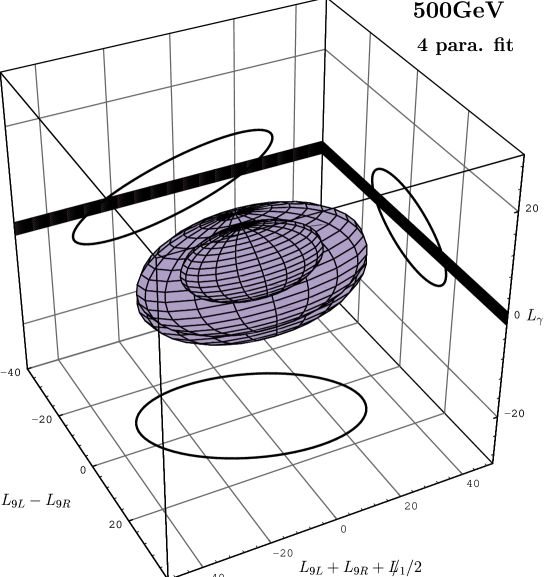
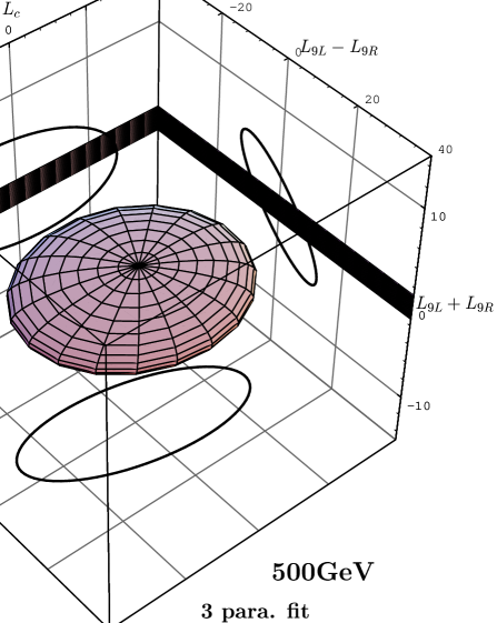
Figure 3: The tri-dimensional bounds in the case of 4 parameters for a fit at $\sqrt{s}=500$GeV ( $\sqrt{s_{\gamma\gamma}}=400$GeV). The ellipsoide represents the $e^{+}e^{-}\;$bound with the ellipses being the projections in the different planes. The limit from $\gamma\gamma$ with unpolarised photons consist of two wafers (planes) whose projections on the planes ($L_{\gamma}$-$L_{V}$) and ($L_{\gamma}$-$L_{9L}+L_{9R}-L\kern-4.49997pt{/}_{1}/2$) are shown. The two “ $\gamma\gamma$ wafers” should be visualised as cutting through the ellipsoid. The lower figure is the result of a 3-parameter fit with $L\kern-4.49997pt{/}_{1}=0$. All results are at $95\%$CL.

In the case where we allow a global $SU(2)$ breaking with $L\kern-4.49997pt{/}_{1}\neq 0$, we have preferred to visualise our results by using the set of independent variables $L_{\gamma}=L_{9L}+L_{9R}+4L\kern-4.49997pt{/}_{1}$ (representing the $\gamma\gamma$ direction), $L_{V}=L_{9L}-L_{9R}$ (this would be zero in a vectorial model on the mould of a scaled up QCD ) and the orthogonal combination ($\sim L_{9L}+L_{9R}-L\kern-4.49997pt{/}_{1}/2$).

Figure 4: a 2D comparison between $\gamma\gamma\rightarrow W^{+}W^{-}\;$and $e^{+}e^{-}\rightarrow W^{+}W^{-}\;$at 500GeV. The ellipses are the results from $e^{+}e^{-}\rightarrow W^{+}W^{-}\;$, with the smaller ellipse corresponding to a fit with two parameters ($L_{9L},L_{9R}$) while the larger one is for the case of three parameters ($L_{9L},L_{9R},L_{c}$). The diagonal band is from $\gamma\gamma\rightarrow W^{+}W^{-}\;$(unpolarised photons). The “bars” along the axes are the one-parameter fits. The thinner ones (inside the box) are for $e^{+}e^{-}\;$and the thicker ones (outside the box) are for $\gamma\gamma$ . All results are at $95\%$CL.

For $e^{+}e^{-}\;$at $500$GeV and with a full 4-parameter fit, one sees (Fig.3) that the limits from $e^{+}e^{-}\rightarrow W^{+}W^{-}\;$lead to relatively loose bounds that are not competitive with what one obtains from the $\gamma\gamma$ mode. In fact the parameter space allows couplings of ${\cal{O}}(10)$ and hence it is doubtful that such analysis will usefully probe symmetry breaking. Even upon switching off the SU(2) violating coupling $L\kern-4.49997pt{/}_{1}$, the multi-parameter bound (Fig.3) obtained from $e^{+}e^{-}\rightarrow W^{+}W^{-}\;$does not compare well with the stringent bounds that one is able to reach in $\gamma\gamma\rightarrow W^{+}W^{-}\;$. Even though, in this case $\gamma\gamma\rightarrow W^{+}W^{-}\;$is blind to $L_{c}$, the bound on $L_{c}$ from $e^{+}e^{-}\;$is not strong enough to be useful ($|L_{c}|<20$). At this energy the benefits of $\gamma\gamma\rightarrow W^{+}W^{-}\;$are very desirable, since when combined with the limits from $e^{+}e^{-}\rightarrow W^{+}W^{-}\;$the parameter space shrinks considerably, even if with little effect on the limit on $L_{c}$. At this energy even in the case of maintaining an exact global SU(2) symmetry with only the parameters ($L_{9L},L_{9R}$) remaining, the $L_{9}$ bound is sensibly reduced if one takes advantage of the $\gamma\gamma$ mode(Fig.4). Note however that the limits from a maximum likelihood fit in $e^{+}e^{-}\rightarrow W^{+}W^{-}\;$, with an integrated luminosity of $\int{\cal L}=20fb^{-1}$ lead to $|L_{9R}|<7\;\;-\;|L_{9L}|<4$; with a slight degradation if one had included $L_{c}$ into the fit. As can be seen from Eq. 3.2, $L_{c}$ does not contribute to the sensitive $W_{L}W_{L}$ direction which benefits the most from the enhanced coupling.

What about if only one parameter were present? In this case both $e^{+}e^{-}\rightarrow W^{+}W^{-}\;$and $\gamma\gamma\rightarrow W^{+}W^{-}\;$give excellent limits as in Fig. 4. $\gamma\gamma$ give slightly better limits, especially in the case of $L_{9R}$ where we gain a factor of two in $\gamma\gamma$ . Note however that this result is obtained without the inclusion of the photon spectra. The latter affects much more the effective $\gamma\gamma$ luminosity than the $e^{+}e^{-}\;$. If one includes a luminosity reduction factor of 10 in the comparison, the results of single-parameter fits would be essentially the same in the two modes. At 500GeV, polarisation in $\gamma\gamma$ has almost no effect for this physics. It should however be kept in mind that in $e^{+}e^{-}\rightarrow W^{+}W^{-}\;$right-handed polarisation would be welcome in fits including $L_{9R}$[29, 15, 16].

As the energy increases, the role of polarisation in $\gamma\gamma$ becomes important, as we detailed in the previous section (see Table 1). However the benefits of $\gamma\gamma\rightarrow W^{+}W^{-}\;$turn out to be rather mitigated, in the sense that combining the results from $\gamma\gamma\rightarrow W^{+}W^{-}\;$to those obtained in $e^{+}e^{-}\rightarrow W^{+}W^{-}\;$does not considerably reduce the bounds one deduces from $e^{+}e^{-}\rightarrow W^{+}W^{-}\;$alone, see Figs. 5- 8. This is especially true at 2TeV, where in the case of a 4-parameter fit, the $\gamma\gamma$ limits reduce the bounds slightly only if the $\gamma\gamma$ are in the correct polarisation setting ($J_{Z}=0$) (see Figs. 7-8). At 2TeV even if one allows a three parameter fit with $L_{c}$ ($L_{9}$), an unpolarised $\gamma\gamma$ collider does not bring any further constraint and one gains only if one combines polarised $\gamma\gamma$ beams with ML methods (Fig. 8). For the case of a one-parameter fit our results indicate, that if one has the same luminosity in the $e^{+}e^{-}\;$and $\gamma\gamma$ modes than there is practically no need for $\gamma\gamma\rightarrow W^{+}W^{-}\;$even when the photon beams are polarised (Fig. 8).

                                               

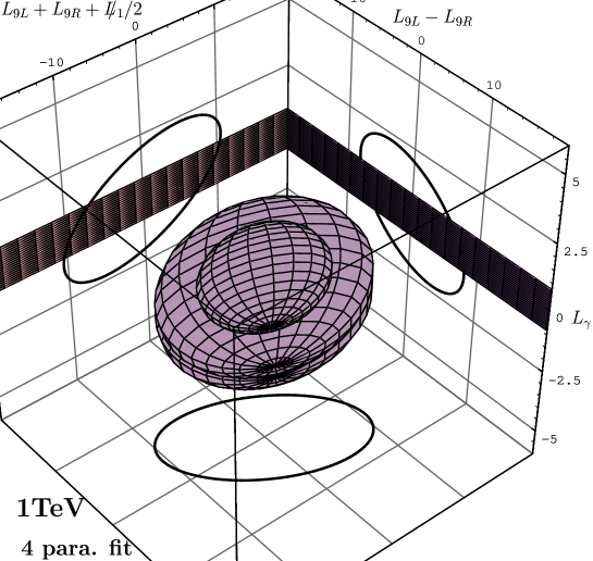
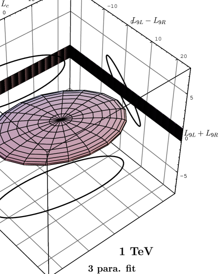
Figure 5: As in fig. 3 but for $\sqrt{s}=1$TeV.

Figure 6: As fig. 4. but with the dashed bands representing the unpolarised result in $\gamma\gamma$ . The additional bands are for the case $J_{Z}=0$ ($++$).

                                               

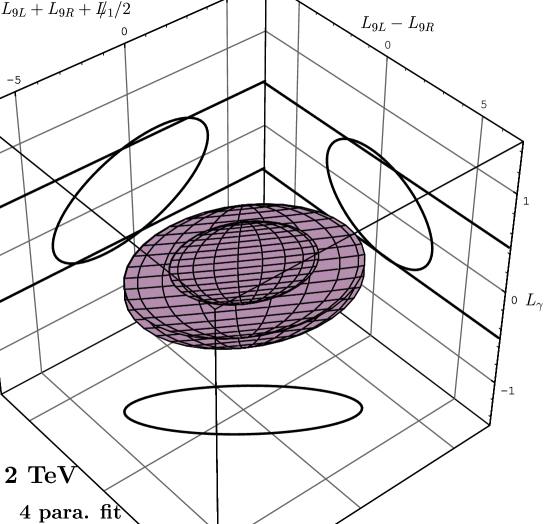
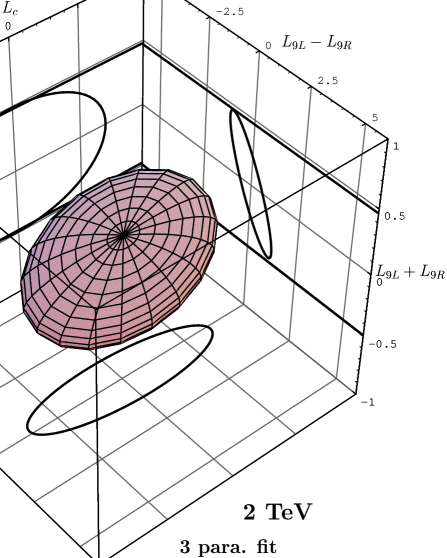
Figure 7: As in fig. 3 but for $\sqrt{s}=2$TeV.

Figure 8: As fig. 6

6 Conclusions

We have critically analysed the usefulness of the $\gamma\gamma$ mode of the next linear collider in probing models of symmetry breaking through the effects of anomalous couplings in the reaction $\gamma\gamma\rightarrow W^{+}W^{-}\;$. To take full advantage of all the information provided by the different helicity amplitudes we have taken into account all the contributions to the full four-fermion final states and studied the approximation based on the “resonant” $W^{+}W^{-}$ final state with complete spin correlations. One of our results is that exploiting the full information provided by the kinematical variables of the 4-fermion variables, as made possible through a fit based on the maximum likelihood method, not only does one obtain excellent limits on the anomalous couplings but we improve considerably on the limit extracted at the level of $\gamma\gamma\rightarrow W^{+}W^{-}\;$. Especially as the energy increases (beyond $500$GeV) these limits are further improved if use is made of polarising the photon beams in a $J_{Z}=0$ setting. One limitation of the $\gamma\gamma$ mode is that within our effective Lagrangian, $\gamma\gamma\rightarrow W^{+}W^{-}\;$only probes one collective combination of operators, that contribute to the magnetic moment of the $W$ (usually refered to as $\Delta\kappa_{\gamma}$). Disentangling between different operators that could point to different mechanisms of symmetry breaking is therefore not possible. We have therefore addressed the question of how this information compares to what we may learn from the normal mode of the linear collider, $e^{+}e^{-}\;$, and whether combining the results of the two modes further constrains the models. In order to conduct this comparison we have relied on the complete calculation of the full 4-fermion final state in $e^{+}e^{-}\;$and used the same analysis (based on the maximum likelihood method) as the one in $\gamma\gamma$ . It turns out that up to 1TeV and in case we allow for more than one anomalous coupling, there is some benefit (especially at 500GeV) in having a $\gamma\gamma$ mode for this type of physics. However for all energies, if one only considers one anomalous coupling, there is very little or no improvement brought about by the $\gamma\gamma$ mode over the $e^{+}e^{-}\;$mode. Considering that our analysis has not taken into account the folding with the luminosity functions which will lead to a reduced effective luminosity in the $\gamma\gamma$ mode, there seems that for one parameter fit there is no need for a $\gamma\gamma$ mode. At much higher energies (2 TeV) this conclusion holds even for multi-parameter fits.

Appendix

A Helicity amplitudes for $\gamma\gamma\rightarrow W^{+}W^{-}\;$

A.1 Tree-level helicity amplitudes for $\gamma\gamma\rightarrow W^{+}W^{-}$ in the ${\cal{S}}{\cal{M}}\;$

To understand the characteristics of the $WW$ cross-section it is best to give all the helicity amplitudes that contain a maximum of information on the reaction. It is important to specify our conventions. We work in the centre of mass of the incoming photons and refrain from making explicit the azimuthal dependence of the initial state. The total energy is $\sqrt{s}$. We take the photon with helicity $\lambda_{1}$ ($\lambda_{2}$) to be in the $+z$ ($-z$) direction and the outgoing $W^{-}$ ($W^{+}$) with helicity $\lambda_{-}$ ($\lambda_{+}$)and 4-momentum $p_{-}$ $p_{+}$:

$$p_{\mp}^{\mu}=\frac{\sqrt{s}}{2}(1,\pm\beta\sin\theta,0,\pm\beta\cos\theta)$$ (A.1)

In the following all $\lambda_{i}=\pm$. The polarisations for the helicity basis are defined as

$$\epsilon_{1}^{\mu}(\lambda_{1})=\frac{1}{\sqrt{2}}(0,-\lambda_{1},-i,0)\;\;\;\;\;\;\;\;\; \epsilon_{2}^{\mu}(\lambda_{2})=\frac{1}{\sqrt{2}}(0,\lambda_{2},-i,0)$$ (A.2)

$$\epsilon_{3}^{\mu}(\lambda_{-})^{*}=\frac{1}{\sqrt{2}}(0,-\lambda_{-}\cos\theta,i,\lambda_{-}\sin\theta) \epsilon_{4}^{\mu}(\lambda_{+})^{*}=\frac{1}{\sqrt{2}}(0,\lambda_{+}\cos\theta,i,-\lambda_{+}\sin\theta)$$

$$\epsilon_{3}^{\mu}(0)^{*}=\frac{\sqrt{s}}{2M_{W}}(\beta,\sin\theta,0,\cos\theta)\;\;\;\;\;\;\;\;\; \epsilon_{4}^{\mu}(0)^{*}=\frac{\sqrt{s}}{2M_{W}}(\beta,-\sin\theta,0,-\cos\theta)$$

We obtain for the tree-level ${\cal{S}}{\cal{M}}\;$helicity amplitudes:

$${\cal M}_{\lambda_{1}\lambda_{2};\lambda_{-}\lambda_{+}}=\frac{4\pi\alpha}{1-\beta^{2}\cos^{2}\theta}\;\;{\cal N}_{\lambda_{1}\lambda_{2};\lambda_{-}\lambda_{+}}\;\;\;;\;\;\;\beta=\sqrt{1-4/\gamma}\;;\;\gamma=s/M_{W}^{2}$$ (A.3)

where

$${\cal N}_{\lambda_{1}\lambda_{2};00} = \;-\;\frac{1}{\gamma}\left\{-4(1+\lambda_{1}\lambda_{2})+(1-\lambda_{1}\lambda_{2})(4+\gamma)\sin^{2}\theta\right\}$$

$${\cal N}_{\lambda_{1}\lambda_{2};\lambda_{-}0} = \sqrt{\frac{8}{\gamma}}\;\;(\lambda_{1}-\lambda_{2})(1+\lambda_{1}\lambda_{-}\cos\theta)\sin\theta\;$$

$${\cal N}_{\lambda_{1}\lambda_{2};0,\lambda_{+}} = \;-\;\sqrt{\frac{8}{\gamma}}\;\;(\lambda_{1}-\lambda_{2})(1-\lambda_{1}\lambda_{+}\cos\theta)\sin\theta\;$$

$${\cal N}_{\lambda_{1}\lambda_{2};\lambda_{-}\lambda_{+}} = \beta(\lambda_{1}+\lambda_{2})(\lambda_{-}+\lambda_{+})+\frac{1}{2\gamma}\left\{-8\lambda_{1}\lambda_{2}(1+\lambda_{-}\lambda_{+})+\gamma(1+\lambda_{1}\lambda_{2}\lambda_{-}\lambda_{+})(3+\lambda_{1}\lambda_{2})\right.$$ (A.4)

$$+ \left.2\gamma(\lambda_{1}-\lambda_{2})(\lambda_{-}-\lambda_{+})\cos\theta-4(1-\lambda_{1}\lambda_{2})(1+\lambda_{-}\lambda_{+})\cos^{2}\theta\right.$$

$$+ \left.\gamma(1-\lambda_{1}\lambda_{2})(1-\lambda_{-}\lambda_{+})\cos^{2}\theta\right\}$$

With the conventions for the polarisations, the fermionic tensors are defined as in [12]. In particular one expresses everything with respect to the $W^{-}$ where the arguments of the $D$ functions refer to the angles of the particle (electron not anti-neutrino), in the rest-frame of the $W^{-}$. The D-functions to use are therefore $D^{W^{-}}_{\lambda,\lambda^{\prime}}(\theta^{*},\phi^{*})\equiv D_{\lambda,\lambda^{\prime}}$, satisfying $D_{\tau_{1},\tau_{2}}=D_{\tau_{2},\tau_{1}}^{*}\;\;\tau_{i}=\pm,0$

$$D_{+,-}=\frac{1}{2}(1-\cos^{2}\theta^{*})e^{2i\phi^{*}} D_{\lambda,0}=-\frac{1}{\sqrt{2}}(1-\lambda\cos\theta^{*})\sin\theta^{*}e^{i\lambda\phi^{*}}$$ (A.5)

$$D_{\lambda,\lambda}=\frac{1}{2}(1-\lambda\cos\theta^{*})^{2} D_{0,0}=\sin^{2}\theta^{*}$$

A.2 Helicity amplitudes for $\gamma\gamma\rightarrow W^{+}W^{-}$ due to the anomalous couplings

For completeness we give the helicity amplitudes for both the coupling $\Delta\kappa_{\gamma}$ that emerges within the effective operators we have studied, as well as the coupling $\lambda_{\gamma}$. The latter contributes also to the quartic $\gamma\gamma WW$ vertex. We also keep the quadratic terms in the anomalous couplings.

The reduced amplitude ${\cal N}^{ano}_{\lambda_{1}\lambda_{2}\lambda_{-}\lambda_{+}}$ is defined in the same way as the ${\cal{S}}{\cal{M}}\;$ones, i.e. in Eq. A.3, ${\cal N}^{sm}\rightarrow{\cal N}^{ano}$

$${\cal N}^{ano}_{++;00} = \Delta\kappa(\gamma\sin^{2}\theta+4\cos^{2}\theta)+4\lambda_{\gamma}\sin^{2}\theta+\Delta\kappa\lambda_{\gamma}(1-3\cos^{2}\theta)$$

$$\frac{\Delta\kappa^{2}}{2}(\gamma\sin^{2}\theta-1+3\cos^{2}\theta)+\frac{\lambda_{\gamma}^{2}}{4}(1+\cos^{2}\theta)(\gamma\sin^{2}\theta+4\cos^{2}\theta-2)$$

$${\cal N}^{ano}_{+-;00} = -\biggl{\{}4\Delta\kappa+\frac{\Delta\kappa^{2}}{4}(\gamma+2)+\frac{\Delta\kappa\lambda_{\gamma}}{2}(\gamma-2)+\frac{\lambda_{\gamma}^{2}}{4}[(\gamma-4)\cos^{2}\theta+2]\biggr{\}}\sin^{2}\theta$$

$${\cal N}^{ano}_{++;\lambda_{3}0} = \frac{\cos\theta\sin\theta}{\sqrt{2\gamma}}\biggl{\{}-\Delta\kappa\left[\gamma\beta+\lambda_{-}(\gamma-4)\right]-\lambda_{\gamma}\left[\gamma\beta+\lambda_{-}(\gamma+4)\right]-$$

$$\frac{\Delta\kappa^{2}}{2}\left[\gamma\beta+\lambda_{-}(\gamma-2)\right]+\frac{\lambda_{\gamma}^{2}}{8}\left[\gamma(\lambda_{-}-\beta)(\gamma-4)\sin^{2}\theta+8\lambda_{-}\right]-$$

$$\Delta\kappa\lambda_{\gamma}\lambda_{-}(\gamma+2)\biggr{\}}$$

$${\cal N}^{ano}_{+-;\lambda_{3}0} = \frac{\sin\theta}{\sqrt{2\gamma}}(1+\lambda_{-}\cos\theta)\biggl{\{}\Delta\kappa(\gamma+4)+\lambda_{\gamma}(\gamma-4)+$$

$$\frac{\Delta\kappa\lambda_{\gamma}}{4}(\gamma-2)(\gamma-(\gamma-4)\cos\theta\lambda_{-})+\frac{\Delta\kappa^{2}}{4}\biggl{\{}3\gamma-(\gamma-4)\lambda_{-}\cos\theta\biggr{\}}+$$

$$\frac{\lambda_{\gamma}^{2}}{8}\bigl{[}\gamma(\gamma-2)(1-\lambda_{-}\cos\theta)^{2}+2\lambda_{-}\gamma\cos\theta(1-\lambda_{-}\cos\theta)+8\cos^{2}\theta\bigr{]}\biggr{\}}$$

$${\cal N}^{ano}_{++;\lambda_{3}\lambda_{4}} = 2\Delta\kappa P^{+}_{34}\left[2+\beta\lambda_{-}(1+\cos^{2}\theta)\right]+$$

$$+\lambda_{\gamma}\biggl{\{}\sin^{2}\theta(\gamma-2)-P^{+}_{34}\left[\beta\lambda_{-}\left(\gamma\sin^{2}\theta+2(1+\cos^{2}\theta)\right)-4\cos^{2}\theta\right]\biggr{\}}+$$

$$\frac{\Delta\kappa^{2}}{8}\biggl{\{}P^{+}_{34}\left[\gamma\sin^{2}\theta-\beta\lambda_{-}(\gamma\sin^{2}\theta-4\cos^{2}\theta)+6(1+\cos^{2}\theta)\right]+2P^{-}_{34}\sin^{2}\theta\biggr{\}}+$$

$$+\frac{\Delta\kappa\lambda_{\gamma}}{4}\biggl{\{}P^{+}_{34}\left[(\gamma\sin^{2}\theta+4\cos^{2}\theta)(1-\beta\lambda_{-})-6\sin^{2}\theta\right]+2P^{-}_{34}(\gamma-1)\sin^{2}\theta\biggr{\}}+$$

$$\frac{\lambda_{\gamma}^{2}}{16}\Biggl{(}P^{+}_{34}(1-\beta\lambda_{-})\left[\gamma(\gamma-2)(3-\cos^{2}\theta)\sin^{2}\theta+2\cos^{2}\theta(5\gamma-\gamma\cos^{2}\theta-4)\right]$$

$$-2\sin^{2}\theta(\gamma-2)(\sin^{2}\theta+2P^{+}_{34})-4\cos^{2}\theta(\sin^{2}\theta+4P^{+}_{34})\Biggr{)}$$

$${\cal N}_{+-;\lambda_{3}\lambda_{4}} = \frac{\Delta\kappa}{2}\left[P^{+}_{34}\sin^{2}\theta+P^{-}_{34}(1+\lambda_{-}\cos\theta)^{2}\right]+\lambda_{\gamma}P^{+}_{34}(\gamma-4)\sin^{2}\theta+$$ (A.8)

$$\frac{\Delta\kappa^{2}}{8}\Bigl{\{}6P^{+}_{34}\sin^{2}\theta+P^{-}_{34}(1+\lambda_{-}\cos\theta)^{2}(\gamma+2-(\gamma-4)\lambda_{-}\cos\theta)\Bigr{\}}+$$

$$\frac{\Delta\kappa\lambda_{\gamma}}{16}\Bigl{\{}2P^{+}_{34}\sin^{2}\theta(\gamma-3)+P^{-}_{34}(1+\lambda_{-}\cos\theta)^{2}(\gamma-2-(\gamma-4)\lambda_{-}\cos\theta)\Bigr{\}}+$$

$$\frac{\lambda_{\gamma}^{2}}{16}\Biggl{\{}2P^{+}_{34}\sin^{2}\theta[2-\sin^{2}\theta(\gamma-4)]+P^{-}_{34}(1+\lambda_{-}\cos\theta)^{2}\times$$

$$\biggl{[}\gamma^{2}(1-\lambda_{-}\cos\theta)(3-\lambda_{-}\cos\theta)-4(1-6\lambda_{-}\cos\theta+2\cos^{2}\theta)-$$

$$2\gamma(6-11\lambda_{-}\cos\theta+3\cos^{2}\theta)\biggr{]}\Biggr{\}}$$

where $P^{\pm}_{34}=(1\pm\lambda_{-}\lambda_{+})/2$ are operators projecting onto the W states with same (opposite) helicities respectively. The amplitudes not written explicitly above are simply obtained with the relation,

$${\cal M}_{\lambda_{1}\lambda_{2};\lambda_{-}\lambda_{+}}={\cal M}^{*}_{-\lambda_{1}-\lambda_{2};-\lambda_{-}-\lambda_{+}}\;\;\;\;\theta\rightarrow-\theta$$ (A.9)

Apart for various signs due to a different labeling of the polarisation vectors, these amplitudes agree with those of Yehudai[30] save for the dominant term (in $s_{\gamma\gamma}$) in the $\lambda_{\gamma}^{2}$ term of the $J_{Z}=0$ amplitude for transverse W’s, i.e. $(1-3\cos^{2}\theta)\rightarrow(3-\cos^{2}\theta)$. This is probably just a misprint.

B Properties of the helicity amplitudes for $e^{+}e^{-}\rightarrow W^{+}W^{-}\;$

The helicity amplitudes for $e^{+}e^{-}\rightarrow W^{+}W^{-}\;$in the presence of tri-linear couplings have been derived repeatedly by allowing for all possible tri-linear couplings. For our purposes we will take the high energy limit ($s\geq M_{W}^{2},M_{Z}^{2}$). Moreover, to easily make transparent the weights of the different operators in the different helicity amplitudes we will further assume $sin^{2}\theta_{W}\simeq 1/4$. This can also help explain the order of magnitudes of the limits we have derived on the anomalous couplings from our maximum likelihood fit based on the exact formulae. Keeping the same notations as those for $\gamma\gamma$ but with the electron polarisation being denoted by $\sigma/2$ with $\sigma=\pm$ ($-$ is for a left-handed electron) and the fact that the electron and positron have opposite helicities, we obtain the very compact formulae for the helicity amplitudes due to the chiral Lagragian parameters. $\theta$ is the angle between the $e^{-}$ and $W^{-}$. For the anomalous, the helicity amplitudes may be approximated as

$${\cal M}^{{\rm ano}}_{-;00} \sim 4\pi\alpha\times \;\gamma\;\sin\theta\;\left\{l_{9}+4\tilde{l}_{1}+\frac{1}{3}r_{9}\right\}$$

$${\cal M}^{{\rm ano}}_{+;00} \sim 4\pi\alpha\times \;\gamma\;\sin\theta\;\left\{\frac{2}{3}r_{9}\right\}$$

$${\cal M}^{{\rm ano}}_{-;\lambda 0} \sim 4\pi\alpha\times \;\sqrt{\frac{\gamma}{2}}\;\frac{(1-\lambda\cos\theta)}{2}\;\left\{\frac{10}{3}l_{9}+4\times 2\tilde{l}_{1}+\frac{2}{3}r_{9}+\lambda g_{5}^{Z}\right\}$$

$${\cal M}^{{\rm ano}}_{+;\lambda 0} \sim 4\pi\alpha\times \sqrt{\frac{\gamma}{2}}\;\frac{(1+\lambda\cos\theta)}{2}\;\left\{\frac{4}{3}\left(l_{9}+r_{9}\right)+\lambda g_{5}^{Z}\right\}$$

$${\cal M}^{{\rm ano}}_{-;\lambda\lambda} \sim-4\pi\alpha\times \;\sigma\;\sin\theta\;\left\{\frac{4}{3}l_{9}\right\}$$ (B.1)

As for the tree-level ${\cal{S}}{\cal{M}}\;$amplitudes within the same approximations one has

$${\cal M}_{-;00}^{{\cal{S}}{\cal{M}}\;} \sim-4\pi\alpha\times \;\sin\theta\;\left\{\frac{14}{3}\right\}$$

$${\cal M}_{+;00}^{{\cal{S}}{\cal{M}}\;} \sim-4\pi\alpha\times \;\sin\theta\;\left\{\frac{2}{3}\right\}$$

$${\cal M}_{-;\lambda-\lambda}^{{\cal{S}}{\cal{M}}\;} \sim 4\pi\alpha\times \;2\lambda\frac{\sin\theta(1-\lambda\cos\theta)}{1-\cos\theta)}$$ (B.2)

The remaining amplitudes all vanish as $1/\sqrt{\gamma}$ or faster, for example one has

$${\cal M}_{-;\lambda 0}^{{\cal{S}}{\cal{M}}\;} \sim-4\pi\alpha\times \;2\sqrt{\frac{2}{\gamma}}\left\{\frac{5}{3}-\frac{1+\lambda}{1-\cos\theta}\right\}\;(1-\lambda\cos\theta)$$ (B.3)

There are a few important remarks. Most importantly, both for a left-handed electron as well as for a right-handed electron there is effective interference in the production of two longitudinal $W_{L}$’s, since the enhancement factor $\gamma$ does not drop out in ${\cal M}_{\mp;00}^{{\cal{S}}{\cal{M}}\;}\times{\cal M}^{{\rm ano}}_{\mp;00}$. This also means that this enhancement factor will be present even in the total cross section for $e^{+}e^{-}\rightarrow W^{+}W^{-}\;$. Since $g_{5}^{Z}$ affects primarily $W_{L}W_{T}$ production it only comes with the enhancement factor $\sqrt{\gamma}$. Moreover this factor will drop out at the level of the diagonal density matrix elements, i.e., at the level of $e^{+}e^{-}\rightarrow W^{+}W^{-}\;$. Thus, it will not be constrained as well as the $L_{i}$’s. In order to improve the limits on $g_{5}^{Z}$ one should exploit the non-diagonal elements. These non diagonal elements also improve the limits on the $L_{i}$ by taking advantage of the large ${\cal{S}}{\cal{M}}\;$amplitude associated with the production of a right-handed $W^{-}$ in association with a left-handed $W^{+}$ (${\cal M}_{-;\lambda-\lambda}$). We note that with a right-handed electron polarisation one would not be able to efficiently reach $L_{9L}$, since only $L_{9R}$ contribute to $W_{L}W_{L}$. Even for $L_{9R}$, considering that the yield with a right-handed electron is too small, statistics will not allow to set a good limit on this parameter. Nevertheless one could entertain the possibility of isolating the effect $g_{5}^{Z}$ with right-handed electrons by considering a forward-backward asymmetry as suggested by Dawson and Valencia[31]. However this calls for an idealistic $100\%$ right-handed polarisation which, moreover leads to a small penalising statistics. Therefore, we had better revert to a fit of the non-diagonal elements in the left-handed electron channel (or the unpolarised beams) case.
Considering the fact that at high energy the $L_{i}$ contribute preponderantly to ${\cal M}^{{\rm ano}}_{-;00}$, one expects any fit to give the best sensitivity on the combination given approximately by $(l_{9}+4\tilde{l}_{1}+\frac{1}{3}r_{9})$. This is well confirmed by our exact detailed maximum likelihood fit performed on the 4-fermion final state.

References

-
[1]
For reviews see:
Proc. of the Workshop on Collisions at GeV: The Physics Potential, ed. P. Zerwas, DESY-92-123A,B (1992) .
ibid DESY-93-123C (1993) and DESY-96-123D (1996).
Proceedings of the LCW95, Physics and Experiments with Linear Colliders, Morioka, Japan, Sep. 1995, Edts Miyamoto et al., World Scientific, 1996.
H. Murayama and M. Peskin, hep-ex/9606003. -
[2]
I.F. Ginzburg, G.L. Kotkin, V.G. Serbo and V.I. Telnov, Sov. ZhETF Pis’ma
34 (1981) 514 [JETP Lett. 34 491 (1982)];
I.F. Ginzburg, G.L. Kotkin, V.G. Serbo and V.I. Telnov, Nucl. Instrum. Methods 205 (1983) 47;
I.F. Ginzburg, G.L. Kotkin, S.L. Panfil, V.G. Serbo and V.I. Telnov, ibid 219 (1984) 5;
V.I. Telnov, ibid A294 (1990) 72;
V.I. Telnov, Proc. of the Workshop on “Physics and Experiments with Linear Colliders”, Saariselkä, Finland, eds. R. Orawa, P. Eerola and M. Nordberg, World Scientific, Singapore (1992) 739;
V.I. Telnov, in Proceedings of the IXth International Workshop on Photon-Photon Collisions., edited by D.O. Caldwell and H.P. Paar, World Scientific, (1992) 369. -
[3]
J.F. Gunion and H.E. Haber, in Research Directions for the Decade, Proc.
of the 1990 DPF Summer Study on High Energy Physics, Snowmass, July 1990,
edited by E.L. Berger, World Scientific, Singapore, p. 469.
ibid, Phys. Rev. D48 (1993) 5109. - [4] B. Grzadkowski and J.F. Gunion, Phys. Lett. B294 (1992) 361.
- [5] M. Krämer, J. Kühn, M. L. Stong and P. M. Zerwas, Z. Phys. C64 (1994) 21.
-
[6]
G. Gounaris and F. M. Renard, Phys. Lett. B236 (1994) 131; ibid Z. Phys. C59 (1993) 143.
K. Hagiwara and M.L Stong, Z. Phys. C62 (1994) 99.
G. Gounaris, F. M. Renard and N. D. Vlachos, Nucl. Phys. B459 (1996) 51. - [7] M. Baillargeon, G. Bélanger and F. Boudjema, in Proceedings of Two-photon Physics from DANE to LEP200 and Beyond, Paris, eds. F. Kapusta and J. Parisi, World Scientific, 1995 p. 267; hep-ph/9405359.
-
[8]
G.V. Jikia, Phys. Lett. B298 (1993) 224; Nucl. Phys. B405 (1993) 24
B. Bajc, Phys. Rev. D48 (1993) 1907
M.S. Berger, Phys. Rev. D48 (1993) 5121
D.A. Dicus and C. Kao, Phys. Rev. D49 (1994) 1265
H. Veltman, Z. Phys. C62 (1994) 235. - [9] O.J. P. Eboli, M.C. Gonzalez-Garcia, F. Halzen and D. Zeppenfeld, Phys. Rev. D48 (1993) 1430.
- [10] M. Baillargeon,G. Bélanger and F. Boudjema, Phys. Rev. D51 (1995) 4712 .
- [11] For a list of references on this process, see G. Bélanger and F. Boudjema, Phys. Lett. B288 (1992) 210.
- [12] M. Bilenky, J.L. Kneur, F.M. Renard and D. Schildknecht, Nucl. Phys. 409 (1993) 22.
- [13] R.L. Sekulin, Phys. Lett. B338 (1994) 369.
- [14] For an up-to-date review, see the Triple gauge bosons couplings report, conv. G. Gounaris, J. L Kneur and D. Zeppenfeld, in the LEP2 Yellow Book, p. 525,Vol. 1, Op. cit .
- [15] T.L.Barklow, In the proceedings of the 8th DPF Meeting, Albuquerque, New Mexico, edt. S. Seidel, World Scientific p. 1236 (1995).
- [16] M. Gintner, S. Godfrey and G. Couture, Phys. Rev. D52 (1995) 6249.
- [17] For a recent review on physics at the linear colliders see, F. Boudjema, Proceedings of the Workshop on Physics and Experiments with Linear Colliders, LCW95, Edts. Miyamoto et al.,, p. 199, Vol. I, World Scientific, 1996. ENSLAPP-A-575/96.
- [18] G. Gounaris and C. G. Papadopoulos, Preprint DEMO-HEP-96/04 and THES-TP 96/11. Dec 97. hep-ph/9612378.
- [19] M. Baillargeon, G. Bélanger and F. Boudjema, ENSLAPP-preprint, Jan. 97 ENSLAPP-A-635.
-
[20]
T. Appelquist and C. Bernard, Phys. Rev. D22 (1980) 200; A. Longhitano, Nucl. Phys. B188 (1981) 118.
T. Appelquist, in “Gauge Theories and Experiments at High Energy”, ed. by K.C. Brower and D.G. Sutherland, Scottish Univ. Summer School in Physics, St. Andrews (1980).
A. Falk, M. Luke and E. Simmons, Nucl. Phys. B365 (1991) 523.
B. Holdom, Phys. Lett. B258 (1991) 156.
D. Espriu and M.J. Herrero, Nucl. Phys. B373 (1992) 117.
C.P. Burgess and D. London, Phys. Rev. Lett. 69 (1993) 3428; ibid Phys. Rev. D48 (1993) 4337.
J. Bagger, S. Dawson and G. Valencia, Nucl. Phys. B399 (1993) 364.
D. Espriu and M.J. Herrero, Nucl. Phys. B373 (1992) 117.
F. Feruglio, Int. J. of Mod. Phys. A28 (1993) 4937.
T. Appelquist and G.H. Wu, Phys. Rev. D48 (1993) 3235.
F. Boudjema, in Proceedings of the Workshop on Physics and Experiments with Linear Colliders, eds. F.A. Harris et al.,, World Scientific, 1994, p. 712.
F. Boudjema, Proceedings of the Workshop on Physics and Experiments with Linear Colliders, LCW95, Edts. Miyamoto et al.,, p. 199, Vol. I, World Scientific, 1996. - [21] G. Altarelli, CERN preprint CERN-TH/96-265, Nov. 1996, hep-ph/9611239.
- [22] M. Peskin and T. Takeuchi, Phys. Rev. Lett. 65 (1990) 964.
- [23] T. Inami, C. S. Lim and A. Yamada, Mod. Phys. Lett. A7 (1992) 2789. See also, T. Inami, C. S. Lim in Proceedings of INS Workshop “Physics of , and Collisions at Linear Accelerators, edts Z. Hioki, T. Ishii and R. Najima, p.229, INS-J-181, May 1995.
- [24] R. Casalbuoni et al., Nucl. Phys. B409 (1993) 257.
- [25] F. Feruglio, Int. J. of Mod. Phys. A28 (1993) 4937.
- [26] T. Appelquist and G.H. Wu, Phys. Rev. D48 (1993) 3235.
- [27] K. Hagiwara, R. Peccei, D. Zeppenfeld and K. Hikasa Nucl. Phys. B282 (1987) 253.
- [28] R. Barlow, Statistics, John Wiley, Chichester, 1989.
- [29] M. Baillargeon, in progress.
-
[30]
E. Yehudai, Phys. Rev. D44 (1991) 3434.
E. Yehudai, Ph.D. thesis, August 1991, SLAC-383. -
[31]
S. Dawson and G. Valencia, Phys. Rev. D49 (1994) 2188.
See also, A.A. Likhoded, T. Han and G. Valencia, Phys. Rev. D53 (1995) 4811.