ABSTRACT

An unified flavour model based on U(2) as flavour group is described. Besides to explain the main characteristics of the fermion spectrum, the model is predictive and agrees quantitatively with experimental data in flavour physics.

THE U(2) SYMMETRY

The aim of this exposition is to describe a theory of flavour based on SU(5) or SO(10) as gauge group and U(2) as flavour group. Such an unified theory has been developed by R. Barbieri, L. J. Hall, S. Raby and myself [1] on the basis of previous works by R. Barbieri, G. Dvali and L.J. Hall [2] and R. Barbieri and L. J. Hall [3].

While the structure of the gauge sector of the Standard Model (SM) is well understood in terms of the unification hypothesis, a coherent and complete quantitative explanation of the flavour sector, in particular of fermion masses and mixings is still missing. Ref. [4] is an attempt in this direction. However, besides the bottom quark and $\tau$ lepton mass unification [5, 6], several relations have been noticed in the past, sometimes justified on a theoretical basis, like, e.g., $|V_{us}|\simeq(m_{d}/m_{s})^{1/2}$ [7], $m_{\mu}\simeq 3m_{s}$ and $m_{d}\simeq 3m_{e}$ [8], or $|V_{ub}/V_{cb}|\simeq(m_{u}/m_{c})^{1/2}$ [9], involving the masses and the CKM matrix elements renormalized at the unification scale. In a supersymmetric theory, the flavour problem extends to scalar masses and scalar-fermion mixings, that have to be consistent with experimental limits on Flavour Changing Neutral Current (FCNC) phenomena [10].

In order to explain the “horizontal” relations among masses and mixings, table 1, in terms of coupling constants of order one, we introduce as usual an horizontal symmetry acting in the same way on the family indexes of different SM representations, and we suppose that this symmetry is spontaneously broken by the SM-invariant vacuum expectation values of “flavon” fields.

Table 1: Fermion masses and mixing relations at the unification scale.

$$\begin{array}[]{|c|c|c|c|}\hline\cr{\mathnormal{U}}/{\mathnormal{D}},{\mathnormal{E}}&m_{t}\gg m_{b},m_{\tau}&\raisebox{0.0pt}[15.0694pt][12.05553pt]{$\displaystyle\frac{m_{c}}{m_{t}}\ll\frac{m_{s}}{m_{b}},\frac{m_{\mu}}{m_{\tau}}$}&\raisebox{0.0pt}[15.0694pt][12.05553pt]{$\displaystyle\frac{m_{u}m_{c}}{m_{t}^{2}}\ll\frac{m_{d}m_{s}}{m_{b}^{2}},\frac{m_{e}m_{\mu}}{m^{2}_{\tau}}$}\\ \hline\cr{\mathnormal{D}}/{\mathnormal{E}}&m_{b}\approx m_{\tau}&\raisebox{0.0pt}[15.0694pt][12.05553pt]{$\displaystyle 3\frac{m_{s}}{m_{b}}\approx\frac{m_{\mu}}{m_{\tau}}$}&\raisebox{0.0pt}[15.0694pt][12.05553pt]{$\displaystyle\frac{m_{d}m_{s}}{m^{2}_{b}}\approx\frac{m_{e}m_{\mu}}{m^{2}_{\tau}}$}\\ \hline\cr\hline\cr V_{\textrm{CKM}}&\raisebox{0.0pt}[15.7152pt][12.05553pt]{$\displaystyle|V_{us}|\sim\sqrt{\frac{m_{d}}{m_{s}}}$}&\raisebox{0.0pt}[15.7152pt][12.05553pt]{$\displaystyle|V_{cb}|\sim\frac{m_{s}}{m_{b}}$}&\raisebox{0.0pt}[15.7152pt][12.05553pt]{$\displaystyle\left|\frac{V_{ub}}{V_{cb}}\right|\sim\sqrt{\frac{m_{u}}{m_{c}}}$}\\ \hline\cr\end{array}$$

Instead of considering the possible horizontal symmetries involving all the three families, we limit ourselves to symmetries acting on the two lightest families. Moreover we require that these families are massless in the fermion sector and exactly degenerate in the scalar sector in the limit of unbroken symmetry, as suggested by the smallness of light fermion Yukawa couplings and by the upper limits on FCNC phenomena. The only suitable continuous non abelian unitary group is then U(2). We prefer to consider a non abelian group because the representation structure, and so the theory, is more constrained than in the abelian case, where there is a large freedom in choosing the horizontal quantum numbers. On the contrary, in the U(2) case, the transformation properties of the flavons can be guessed from the requirement of having mixing among the three fermion families.

We do not want direct couplings of the flavon fields $\phi$ to the fermion fields $\psi$ through renormalizable operators. Rather, we suppose that the flavons appear only in non renormalizable effective operators generated below a “flavour scale” $M=\mathcal{O}\left(M_{\mathrm{G}}\div M_{\mathrm{P}}\right)$ at which the physics that mediate the U(2) breaking is integrated out. An example of such a physics is given by the “Froggatt-Nielsen mechanism”, as explained by G. Ross in his lectures [11]. The ratios $\langle\phi\rangle/M$ provide the small parameters needed to describe the fermion mass and mixing structure without using small couplings.

Let us choose the transformation properties of the two light families, $\psi_{a}$, $a=1,2$, under U(2):

$$U\in\mathrm{U(2)}:\;\psi_{a}\rightarrow U_{a}^{b}\psi_{b}$$

(the third family, as the Higgses, is supposed to be U(2)-invariant). Then, in order to generate mixing between the third and the light families, it is necessary to have a flavon field $\phi^{a}$ that transforms in the conjugate way relative to $\psi_{a}$. This flavon gives rise to 12/3 mixing through Yukawa interactions like $(\langle\phi^{a}\rangle/M)\psi_{a}\psi_{3}h$. But $\phi^{a}$ only breaks U(2) to U(1) (at a scale $V$ with $V/M=\mathcal{O}\left(|V_{cb}|_{\mathrm{G}}\right)=\mathcal{O}\left(0.02\right)$) and the U(1) residual symmetry prevents the lightest generation to get mass and to mix with the heavier ones. In order to break U(1) and to generate the operator $\psi_{a}\psi_{b}h$, it is necessary to have a flavon field $\phi^{ab}=A^{ab}+S^{ab}$ with transformation properties under U(2) as indicated by the position of the indexes, where $A^{ab}$ and $S^{ab}$ are their antisymmetric and symmetric irreducible components. Since $\langle A^{ab}\rangle$ breaks U(1) and gives mass to the lightest family, the corresponding scale of breaking $v$ has to be lower than $V$. Moreover, in order to generate the $m_{s}/m_{b}$ ratio at the same scale of $|V_{cb}|$, $S^{ab}$ should break U(2) at the $V$ scale. If we finally suppose that all breakings of U(2) at the $V$ scale leave unbroken the same U(1), we are left with the following breaking pattern (in a suitable basis)

$$\text{U(2)}@>{\left\langle\phi^{a}\right\rangle,\left\langle S^{ab}\right\rangle}>>\text{U(1)}@>{\left\langle A^{ab}\right\rangle}>>\{\mathbf{1}\}$$ (0a)

$$\langle\phi^{a}\rangle=\begin{pmatrix}0\\ V\end{pmatrix},\enspace\big{\langle}A^{ab}\big{\rangle}=\begin{pmatrix}0&v\\ -v&0\end{pmatrix},\enspace\big{\langle}S^{ab}\big{\rangle}=\begin{pmatrix}0&0\\ 0&V^{\prime}\end{pmatrix},$$ (0b)

$$V,v>0,\qquad v\ll V\approx|V^{\prime}|\ll M.$$ (0c)

Also U(2) invariant fields can develop an expectation value and play a role. We denote them with $\Sigma$.

As a consequence of the previous breaking pattern, the Yukawa matrices $\boldsymbol{\lambda}_{{\mathnormal{}}}$ and the scalar masses $\mathbf{m}^{2}$ are in the form

$$\boldsymbol{\lambda}_{{\mathnormal{}}}=\begin{pmatrix}0&\epsilon^{\prime}&0\\ -\epsilon^{\prime}&\epsilon&x\epsilon\\ 0&y\epsilon&1\end{pmatrix}\qquad\mathbf{m}^{2}=\begin{pmatrix}m^{2}_{1}&0&0\\ 0&m^{2}_{1}(1+z\epsilon^{2})&\epsilon{m^{2}_{2}}^{*}\\ 0&\epsilon m^{2}_{2}&m^{2}_{3}\end{pmatrix}$$ (2)

where $\epsilon\equiv V/M$, $\epsilon^{\prime}\equiv v/M$, $x,y,z=\mathcal{O}\left(1\right)$ and $m^{2}_{1},m^{2}_{2},m^{2}_{3}=\mathcal{O}\left(m^{2}_{S}\right)$. This leads to a CKM matrix in the form [12]

$$V_{\text{CKM}}=\begin{pmatrix}c^{{\mathnormal{D}}}_{12}&s^{{\mathnormal{D}}}_{12}-s^{{\mathnormal{U}}}_{12}e^{i\phi}&s^{{\mathnormal{U}}}_{12}s\\ s^{{\mathnormal{U}}}_{12}-s^{{\mathnormal{D}}}_{12}e^{i\phi}&c^{{\mathnormal{D}}}_{12}e^{i\phi}&-c^{{\mathnormal{U}}}_{12}s\\ -s^{{\mathnormal{D}}}_{12}s&c^{{\mathnormal{D}}}_{12}s&e^{-i\phi}\end{pmatrix}$$ (3)

in terms of

$$t^{D}_{12}=\frac{s^{D}_{12}}{c^{D}_{12}}=\sqrt{\frac{m_{d}}{m_{s}}}\qquad t^{U}_{12}=\frac{s^{U}_{12}}{c^{U}_{12}}=\sqrt{\frac{m_{u}}{m_{c}}}$$ (4)

and of the parameters $s>0$ and $\phi\in(0,\pi)$.

The previous form of the CKM matrix is in agreement with the experimental values of $|V_{us}|$ and $|V_{ub}/V_{cb}|$. Moreover, due to the $\epsilon$ term in the $\lambda_{22}$ entry, in the down quark sector we have

$$\frac{m_{s}}{m_{b}}=\mathcal{O}\left(\epsilon\right)=\mathcal{O}\left(|V_{cb}|\right)\quad\text{and}\quad\frac{\tilde{m}^{2}_{d}-\tilde{m}^{2}_{s}}{\tilde{m}^{2}_{d}}\leq\mathcal{O}\left(\epsilon^{2}\right)=\mathcal{O}\left(\frac{m_{s}^{2}}{m_{b}^{2}}\right),$$ (5)

in agreement with the experimental values of $m_{s}/m_{b}$ and $|V_{cb}|$ and with the limits on $(\tilde{m}^{2}_{d}-\tilde{m}^{2}_{s})/\tilde{m}^{2}_{d}$ given by the value of $\epsilon_{K}$, the CP violation parameter in the $K^{0}$-$\bar{K}^{0}$ system [10]. In models in which the 22 entry is vanishing or of order $\epsilon^{2}$ it is on the contrary

$$\frac{m_{s}}{m_{b}}=\mathcal{O}\left(\epsilon^{2}\right)=\mathcal{O}\left(|V_{cb}|^{2}\right)\qquad\frac{\tilde{m}^{2}_{d}-\tilde{m}^{2}_{s}}{\tilde{m}^{2}_{d}}\leq\mathcal{O}\left(\epsilon^{2}\right)=\mathcal{O}\left(\frac{m_{s}}{m_{b}}\right).$$ (6)

The CKM matrix in (3) has been obtained by diagonalizing a Yukawa matrix in the form of eq. (2) in each sector of given charge $U$, $D$, $E$ without comparing the Yukawa matrices of different sectors. By doing that, we immediately see that, to reproduce the suppression of the mass ratios in the $U$-sector relative to the $D$- and $E$-sector ones (“$U/D,E$” line in table 1), the 12, 21 and 22 entries of the $U$-sector Yukawa matrix, $\boldsymbol{\lambda}_{{\mathnormal{U}}}$, have to be suppressed relative to the corresponding entries in $\boldsymbol{\lambda}_{{\mathnormal{D}}}$ and $\boldsymbol{\lambda}_{{\mathnormal{E}}}$. This suppression can be explained in terms of couplings of order one only in presence of vertical relations among the coupling constants as those ones provided by an unified gauge group.

UNIFICATION

Let us then consider the U(2) theory in the case of the minimal unified group SU(5), where each family is represented by a tenplet $T$ and an anti-fiveplet $\bar{F}$. The flavons must transform as ${\boldsymbol{1}}$, ${\boldsymbol{24}}$ or ${\boldsymbol{75}}$ under SU(5), otherwise they cannot have a SM-invariant expectation value or they cannot contribute to the Yukawa matrices linearly. The only renormalizable interactions are then

$$T_{3}T_{3}H,\qquad\bar{F}_{3}T_{3}H,$$ (7)

while the possible non renormalizable interactions at the linear order in the flavons are

$$\bar{F}_{3}T_{a}\bar{H}\frac{\phi^{a}}{M},\qquad\bar{F}_{a}T_{3}\bar{H}\frac{\phi^{a}}{M},\qquad T_{3}T_{a}H\frac{\phi^{a}}{M},$$ (7a)

$$T_{a}T_{b}H\frac{S^{ab}}{M},\qquad T_{a}T_{b}H\frac{A^{ab}}{M},$$ (7b)

$$\bar{F}_{a}T_{b}H\frac{S^{ab}}{M},\qquad\bar{F}_{a}T_{b}H\frac{A^{ab}}{M}.$$ (7c)

The operators $T_{a}T_{b}H\langle S^{ab}\rangle/M$ and $T_{a}T_{b}H\langle A^{ab}\rangle/M$ are responsible for the contributions to $m_{c}/m_{t}$ and $(m_{u}m_{c}/m_{t}^{2})^{1/2}$ at linear order in $\epsilon$, $\epsilon^{\prime}$ respectively. The $m_{c}/m_{t}$ and $(m_{u}m_{c}/m_{t}^{2})^{1/2}$ suppressions can then be explained if this two operators are vanishing and these ratios are generated at second order in the expectation values. Can this happen in a natural way? Let us consider first the operator $T_{a}T_{b}H\langle S^{ab}\rangle/M$. Since only the symmetric part of the product $T_{a}T_{b}$ participates in this interaction, if $S^{ab}$ transforms as ${\boldsymbol{75}}$ under SU(5) the operator $T_{a}T_{b}HS^{ab}/M$ vanishes because it cannot be constructed in a SU(5) invariant way. If $S^{ab}$ is not a ${\boldsymbol{75}}$ of SU(5), the only case in which $T_{a}T_{b}H\langle S^{ab}\rangle/M$ vanishes is when $S^{ab}$ has two components transforming as ${\boldsymbol{1}}$ and ${\boldsymbol{24}}$ respectively, but only for a particular value of the ratio of their expectation values. This possibility has not a natural interpretation in the SU(5) context but has to be taken in consideration when additional vertical structure is present, as it is the case in SO(10).

Analogously, the $T_{a}T_{b}H\langle A^{ab}\rangle/M$ operator vanishes only if $A^{ab}$ is a SU(5) singlet or if $A^{ab}$ has two components transforming as ${\boldsymbol{24}}$ and ${\boldsymbol{75}}$, for a particular value of the ratio of their expectation values.

Thus the SU(5)$\times$U(2) theory allows a natural explanation of the suppression of the $U$-sector mass ratios that requires $S^{ab}\sim{\boldsymbol{75}}$ and $A^{ab}\sim{\boldsymbol{1}}$. It is very interesting that in this case the $D/E$ relations in table 1 are automatically predicted as a consequence of $\lambda^{D}_{33}=\lambda^{E}_{33}$, $\lambda^{D}_{22}=-\frac{1}{3}\lambda^{E}_{22}$, $\lambda^{D}_{12}=\lambda^{E}_{12}$ that follow from the SM decomposition of the operators $\bar{F}_{a}T_{b}\bar{H}\langle S^{ab}\rangle/M$ and $\bar{F}_{a}T_{b}\bar{H}\langle S^{ab}\rangle/M$.

Let us consider now full unification of every single families through SO(10). In this case, the possible representations of the flavons are ${\boldsymbol{1}}$, ${\boldsymbol{45}}$, ${\boldsymbol{54}}$ and ${\boldsymbol{210}}$. It is possible to implement the mechanism described above by using representations for $A^{ab}$ and $S^{ab}$ having components transforming as ${\boldsymbol{1}}$ and ${\boldsymbol{75}}$ respectively under SU(5). In this case, $S^{ab}$ must transform as ${\boldsymbol{210}}$ under SO(10).

On the other hand, it is possible to explain the suppression of the $U$-sector mass ratios using only singlets and adjoints of SO(10). This is possible if $S^{ab}$ is a SO(10) adjoint and if the particular value of the ratio of its components transforming as ${\boldsymbol{1}}$ and ${\boldsymbol{24}}$ under SU(5) is the one characteristic of the $B-L$ generator. Moreover the expectation value of $A^{ab}$ must be SU(5) invariant.

To generate higher order contributions to the fermion masses we use the U(2)-invariant SO(10)-adjoint field $\Sigma$. If we decompose its breaking $\langle\Sigma\rangle$ along the generators $X$ and $Y$, $\langle\Sigma\rangle=\Sigma_{X}+\Sigma_{Y}$, ($X$ and $Y$ generate the SM-invariant generator subspace and are given in table 2) we see that the $D$- and $E$-sector light masses require a ratio $\langle\Sigma_{X}\rangle/M$ not far from 1, while $\langle\Sigma_{Y}\rangle/M=\mathcal{O}\left(0.02\right)$ is responsible for the suppression of the $U$-sector mass ratios. Also in this case the $D/E$ relations in table 1 are automatically predicted, but $\lambda^{D}_{22}=-\lambda^{E}_{22}/3$ becomes $\lambda^{D}_{22}=\lambda^{E}_{22}/3$. The relevant operators are then

$$\psi_{3}f_{1}\left({\Sigma_{X}\over M}\right)H\psi_{3}$$ (8a)

$${1\over M}\psi_{3}\langle\phi^{a}\rangle f_{2}\left({\Sigma_{X}\over M}\right)H\psi_{a}$$ (8b)

$${1\over M}\psi_{a}\left(\big{\langle}S^{ab}\big{\rangle}f_{3}\left({\Sigma_{X}\over M}\right)+\big{\langle}A^{ab}\big{\rangle}f_{4}\left({\Sigma_{X}\over M}\right)\right)H\psi_{b}$$ (8c)

$$\begin{gathered}{1\over M^{2}}\psi_{a}\left(\big{\langle}S^{ab}\big{\rangle}\Sigma_{Y}f_{5}\left({\Sigma_{X}\over M}\right)+\big{\langle}A^{ab}\big{\rangle}\Sigma_{Y}f_{6}\left({\Sigma_{X}\over M}\right)\right)H\psi_{b}\\ +{1\over M^{2}}\psi_{a}\langle\phi^{a}\rangle\langle\phi^{b}\rangle f_{7}\left({\Sigma_{X}\over M}\right)H\psi_{b},\end{gathered}$$ (10a)

where the functions $f$ take into account all orders in $\Sigma_{X}/M$ and we only consider the leading orders in $\Sigma_{Y}/M$.

Table 2: Values of some SM invariant generators on SM representations. $X$ is SU(5) invariant, $Y$ is the hypercharge, $B-L$ the barion minus lepton number and $T_{3R}$ the third component of the right weak isospin.

$$\begin{array}[]{c|cccccc}&{Q}&{u}&{d}&{L}&{\nu}&{e}\\ \hline\cr X&1&1&-3&-3&5&1\\ Y&1/6&-2/3&1/3&-1/2&0&1\\ {B-L}&1/3&-1/3&-1/3&-1&1&1\\ T_{3R}&0&1/2&-1/2&0&1/2&-1/2\end{array}$$

PREDICTIONS OF UNIFIED MODELS

In the unified models described above, the Yukawa matrices are of the form

$$\boldsymbol{\lambda}_{{\mathnormal{U}}}=\begin{pmatrix}0&\epsilon^{\prime}\rho&0\\ -\epsilon^{\prime}\rho&\epsilon\rho^{\prime}&y_{{\mathnormal{U}}}\epsilon\\ 0&x_{{\mathnormal{U}}}\epsilon&1\end{pmatrix}\lambda,\qquad\boldsymbol{\lambda}_{{\mathnormal{(D,E)}}}=\begin{pmatrix}0&\epsilon^{\prime}&0\\ -\epsilon^{\prime}&(1,\pm 3)\epsilon&y_{{\mathnormal{(D,E)}}}\epsilon\\ 0&x_{{\mathnormal{(D,E)}}}\epsilon&1\end{pmatrix}\lambda\zeta,$$ (12)

where $x_{U,D,E}$, $y_{U,D,E}$, $\lambda$, $\rho^{\prime}/\rho$ are of order one, $\epsilon,\rho=\mathcal{O}\left(0.02\right)$, $\epsilon^{\prime}=\mathcal{O}\left(0.004\right)$ and the factor $\zeta=\mathcal{O}\left(0.02\right)$ corresponds to the possibility that the two light Higgs doublets appear in the unified multiplet in the renormalizable Yukawa interaction with different weights. In this way we do not solve the $m_{b}/m_{t}\ll 1$ problem but we reexpress it in term of $\zeta\ll 1$.

From eq. (12), both qualitative and quantitative predictions follow. If we neglect the order one parameters, we can have order of magnitude expressions for the 13 Yukawa observables at the unification scale in terms of 4 small parameters, $\epsilon$, $\rho$, $\epsilon^{\prime}$ and $\zeta$. This gives rise to 9 qualitative or order of magnitude predictions in the Yukawa sector:

$$m_{t}\sim v=174\,\mathrm{GeV}$$ (12a)

$$m_{b}\sim m_{\tau}\quad 3\frac{m_{s}}{m_{b}}\sim\frac{m_{\mu}}{m_{\tau}}\quad\frac{m_{d}m_{s}}{m_{b}^{2}}\sim\frac{m_{e}m_{\mu}}{m_{\tau}^{2}}$$ (12b)

$$\frac{m_{s}}{m_{b}}\sim\left(\frac{m_{c}}{m_{t}}\right)^{1/2}$$ (12c)

$$\left|\frac{V_{ub}}{V_{cb}}\right|\sim\sqrt{\frac{m_{u}}{m_{c}}}\quad\left|\frac{V_{td}}{V_{ts}}\right|\sim\sqrt{\frac{m_{d}}{m_{s}}}$$ (12d)

$$|V_{cb}|\sim\frac{m_{s}}{m_{b}}\qquad J_{\text{CP}}\sim\left(\frac{m_{d}}{m_{s}}\frac{m_{u}}{m_{c}}\right)^{1/2}|V_{cb}|^{2},$$ (12e)

besides $|V_{us}|=\mathcal{O}\left(\sqrt{m_{d}/m_{s}}\right)$.

Let us come now to the quantitative predictions. Taking into account order one factors, from the diagonalization of the Yukawa matrices in eqs. (12) we obtain the 5 following relations:

$$\frac{m_{\mu}}{m_{\tau}}\left(1-\frac{m_{e}}{m_{\mu}}\right)\simeq 3\frac{m_{s}}{m_{b}}\left(1-\frac{m_{d}}{m_{s}}\right)$$ (13a)

$$m_{b}\simeq m_{\tau}\qquad\frac{m_{e}m_{\mu}}{m_{\tau}^{2}}\simeq\frac{m_{d}m_{s}}{m_{b}^{2}}$$ (13b)

$$\left|\frac{V_{ub}}{V_{cb}}\right|\simeq\sqrt{\frac{m_{u}}{m_{c}}}\qquad\left|\frac{V_{td}}{V_{ts}}\right|\simeq\sqrt{\frac{m_{d}}{m_{s}}}.$$ (13c)

Eq. (13aa) has $\mathcal{O}\left(\epsilon\right)$ corrections from the diagonalization, while eqs. (13ab,c) have only $\mathcal{O}\left(\epsilon^{2}\right)$ corrections. All of them, however, have corrections due to possible higher order contributions in $\Sigma_{Y}/M$ or to weak scale radiative corrections, both of order $\mathcal{O}\left(\epsilon\right)$.

The quantitative predictions in eqs. (13a) all agree with the experimental values of the quantities involved. On the other hand these errors are not so small. Nevertheless, as H. Leutwyler explained by his lectures [13], there is a combination of light quark masses that is known with good precision:

$$Q=\frac{m_{s}/m_{d}}{\sqrt{1-(m_{u}/m_{d})^{2}}}=22.7\pm 0.08.$$ (15)

Taking into account $\mathcal{O}\left(\epsilon\right)$ corrections to (13aa) we get our prediction

$$Q\simeq\frac{25}{\sqrt{1-(m_{u}/m_{d})^{2}}}\cdot(1-2\Delta),$$ (16)

with

$$\Delta=\operatorname{Re}\left[\left(x_{{\mathnormal{D}}}y_{{\mathnormal{D}}}\mp\frac{1}{3}x_{{\mathnormal{E}}}y_{{\mathnormal{E}}}\right)\epsilon\right].$$ (17)

The $Q$ value, together with $|V_{cb}|=|(x_{U}-x_{D})\epsilon|$, is then a constraint on the $\mathcal{O}\left(\epsilon\right)$ corrections, that depend on the 23 and 32 entries of the Yukawa matrices and, in turn, on the direction of the $\phi^{a}$ expectation value in the generator space.

It is also possible to test quantitatively the class of considered models by doing a fit of the CKM matrix. Eqs. (3) and (4), that are pure U(2) consequences, allows a parameterization of $V_{\text{CKM}}$ in terms of $s$ and $\phi$, besides $m_{u}/m_{c}$ and $m_{d}/m_{s}$ that, fixing $Q$, $m_{t}$, $m_{b}$, $m_{c}$, can be expressed in terms of $m_{s}$, $\alpha_{s}(M_{Z})$, $m_{u}/m_{d}$. We can then perform a fit of the U(2) model expressing the measured $|V_{us}|$, $|V_{cb}|$, $|V_{ub}/V_{cb}|$, $\alpha_{s}(M_{Z})$, $m_{s}$ in terms of $m_{u}/m_{d}$, $s$, $\phi$, $\alpha_{s}(M_{Z})$, $m_{s}$. In the unified case, $m_{s}$ can be expressed in terms of lepton masses using the relation $m_{e}m_{\mu}=m_{d}m_{s}$ valid at the unification scale. Finally, if we assume that $\epsilon_{K}$ and the $B_{d}$-$\bar{B}_{d}$ mass difference are accounted for by the usual SM diagrams, we can further constrain the fit and extend it to the SM case, in which only the parameterization in (3) is used.

The results of the fit in the unified U(2) models are summarized in table 3. Also, in figure 1 the predictions for the angles $\alpha$, $\beta$ of the unitarity triangle,

$$\alpha=\arg\left(-\frac{V_{tb}^{*}V_{td}}{V_{ub}^{*}V_{ud}}\right)\qquad\beta=\arg\left(-\frac{V_{cb}^{*}V_{cd}}{V_{tb}^{*}V_{td}}\right)\qquad\gamma=\arg\left(-\frac{V_{ub}^{*}V_{ud}}{V_{cb}^{*}V_{cd}}\right)$$ (18)

are shown. In terms of the parameterization of the CKM matrix in (3), these angles turn out to be

$$\alpha =\phi$$ (19)

$$\beta =\arg\left(1-\frac{s^{{\mathnormal{U}}}_{12}}{s^{{\mathnormal{D}}}_{12}}e^{-i\phi}\right)$$ (20)

$$\gamma =\pi-\alpha-\beta.$$ (21)

Table 3: Results of the fit in the unified U(2) theories with (“constrained”) or without (“unconstrained”) inclusion of $\epsilon_{K}$ and $\Delta m_{B_{d}}$ in the inputs.

$$\begin{array}[]{||c|c|c|c||}\hline\cr&\mbox{inputs}&\mbox{constrained}&\mbox{unconstrained}\\ \hline\cr m_{s}/\,\mathrm{MeV}&175\pm 55&153^{+35}_{-22}&153\pm 35\\ |V_{cb}|&0.038\pm 0.004&0.039^{+0.0025}_{-0.0015}&0.038\pm 0.004\\ |V_{ub}/V_{cb}|&0.08\pm 0.02&0.075\pm 0.013&0.075\pm 0.016\\ \epsilon_{K}\cdot 10^{3}&2.26&2.26&\pm(1.7^{+1.3}_{-0.1})\\ B_{K}&0.8\pm 0.2&0.86\pm 0.16&0.8\\ \Delta m_{B_{d}}/\mbox{ps}^{-1}&0.464&0.464&0.37^{+0.14}_{-0.05}\\ \sqrt{B}f_{B}/\,\mathrm{MeV}&200\pm 40&178\pm 18&200\\ \hline\cr\alpha_{s}(M_{Z})&0.117\pm 0.006&0.118\pm 0.005&0.118\pm 0.005\\ \hline\cr\end{array}$$

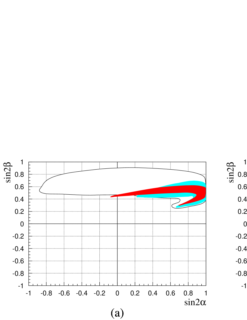
Figure 1: Regions in the $\sin 2\alpha$–$\sin 2\beta$ plane, as determined at the 90% confidence level by the fit in the SM (white area in (a)), in the “pure” U(2) model (grey area) and in the unified U(2) model (dark area), in the “constrained”, (a), and “not constrained”, (b), case.

In conclusion, I briefly summarize the characteristics of the unified U(2) models that we have considered.

• The models are simple and motivated.

• The order of magnitude of 13 fermion masses and mixings are qualitatively understood in terms of 4 small parameters: the ratios of the two U(2) breaking scales and the flavour scale $M$, the ratio of the SU(5) breaking scale and $M$ and the ratio of the coefficients of the light Higgs doublets in the unified Higgs multiplet. The scales are then as shown in figure 2.

  Figure 2: Scales of symmetry breaking vevs appropriate to the SU(5) (a) and SO(10) (b) cases described in the text.

• A quantitative analysis of experimental data is possible in the general model through a successful fit that predicts a strong correlation among the $\alpha$ and $\beta$ angles of the unitarity triangle. Moreover, 5 precise relations among mass and mixings are predicted.

• The suppression of $U$-sector mass ratios is explained in a natural way and automatically leads to the $D/E$ relations in table 1.

• The scalar masses and mixings fulfill the requirements following from the experimental limits on FCNC phenomena. Moreover, they are constrained by U(2) symmetry and unification. This allows an analysis of contributions from supersymmetric particles to several quantities in flavour physics [14].

REFERENCES

[1]
R. Barbieri, L. J. Hall, S. Raby, and A. Romanino,
Unified theories with U(2) flavor symmetry,
hep-ph/9610449.
[2]
R. Barbieri, G. Dvali, and L. J. Hall,
Phys. Lett. B377, 76 (1996).
[3]
R. Barbieri and L. J. Hall,
A grand unified supersymmetric theory of flavor,
hep-ph/9605224.
[4]
G. W. Anderson, S. Raby, S. Dimopoulos, L. J. Hall, and G. D. Starkman,
Phys. Rev. D49, 3660 (1994).
[5]
M. S. Chanowitz, J. Ellis, and M. K. Gaillard,
Nucl. Phys.B128, 506 (1977).
[6]
L. E. Ibanez and C. Lopez, Phys. Lett.126B, 54 (1983);
H. Arason et al., Phys. Rev. Lett.67, 2933 (1991);
A. Giveon, L. J. Hall, and U. Sarid, Phys. Lett.271B, 138
(1991).
[7]
R. Gatto, G. Sartori, and M. Tonin, Phys. Lett.28B, 128
(1968);
N. Cabibbo and L. Maiani, Phys. Lett.28B, 131
(1968);
S. Weinberg, in A Festschrift for I.I. Rabi,
edited by L. Motz, New York Academy of Sciences, 1977.
[8]
H. Georgi and C. Jarlskog, Phys. Lett.86B, 297 (1979).
[9]
J. Harvey, P. Ramond, and D. Reiss, Phys. Lett.92B, 309 (1980).
[10]
For a most recent analysis, see F. Gabbiani, E. Gabrielli, A. Masiero,
and L. Silvestrini,
Nucl. Phys. B477, 321 (1996).
[11]
C. Froggatt and H. B. Nielsen,
Nucl. Phys. B147, 277 (1979);
G. G. Ross, these proceedings.
[12]
L. J. Hall and A. Rasin,
Phys. Lett. B315, 164 (1993).
[13]
H. Leutwyler,
The masses of the light quarks,
Talk given at the Conference on Fundamental Interactions of
Elementary Particles, ITEP, Moscow, Russia, 1995;
H. Leutwyler, these proceedings.
[14]
R. Barbieri, L. J. Hall and A. Romanino, work in progress.