QCD TESTS FROM TAU DECAYS

FTUV/97-03
IFIC/97-03
January 1997

The total $\tau$ hadronic width can be accurately calculated using analyticity and the operator product expansion. The theoretical analysis of this observable is updated to include all available perturbative and non-perturbative corrections. The experimental determination of $\alpha_{s}(M_{\tau}^{2})$ and its actual uncertainties are discussed.

1 Introduction

The inclusive character of the total $\tau$ hadronic width renders possible an accurate calculation of the ratio $\!{}^{{\bf?},{\bf?},{\bf?},{\bf?},{\bf?},{\bf?},{\bf?},{\bf?},{\bf?}}$ [$(\gamma)$ represents additional photons or lepton pairs]

$$R_{\tau}\equiv{\Gamma[\tau^{-}\rightarrow\nu_{\tau}\,\mbox{\rm hadrons}\,(\gamma)]\over\Gamma[\tau^{-}\rightarrow\nu_{\tau}e^{-}{\bar{\nu}}_{e}(\gamma)]},$$ (1)

using standard field theoretic methods. If strong and electroweak radiative corrections are ignored and if the masses of final–state particles are neglected, the universality of the W coupling to the fermionic charged currents implies

$$R_{\tau}\,\simeq\,N_{c}\,(|V_{ud}|^{2}+|V_{us}|^{2})\,\simeq\,3\;,$$ (2)

which compares quite well with the experimental average $\!{}^{{\bf?}}$ $R_{\tau}=3.649\pm 0.014$. This provides strong evidence for the colour degree of freedom $N_{c}$.

The QCD dynamics is able to account quantitatively for the 20% difference between the naïve prediction (2) and the measured value of $R_{\tau}$. Moreover, the uncertainties in the theoretical calculation of $R_{\tau}$ are quite small. The value of $R_{\tau}$ can then be accurately predicted as a function of $\alpha_{s}(M_{\tau}^{2})$. Alternatively, measurements of inclusive $\tau$ decay rates can be used to determine the value of the QCD running coupling $\alpha_{s}(M_{\tau}^{2})$ at the scale of the $\tau$ mass. In fact, $\tau$ decay is probably the lowest–energy process from which the running coupling constant can be extracted cleanly, without hopeless complications from non-perturbative effects. The $\tau$ mass $\!{}^{{\bf?}}$, $M_{\tau}=(1777.00{\,}^{+0.30}_{-0.27})$ MeV, lies fortuitously in a compromise region where the coupling constant $\alpha_{s}(M_{\tau}^{2})$ is large enough that $R_{\tau}$ is sensitive to its value, yet still small enough that the perturbative expansion still converges well. Moreover, the non-perturbative contributions to the total $\tau$ hadronic width are very small.

It is the inclusive nature of the total semihadronic decay rate that makes a rigorous theoretical calculation of $R_{\tau}$ possible. The only separate contributions to $R_{\tau}$ that can be calculated are those associated with specific quark currents. We can calculate the non-strange and strange contributions to $R_{\tau}$, and resolve these further into vector and axial–vector contributions. Since strange decays cannot be resolved experimentally into vector and axial–vector contributions, we will decompose our predictions for $R_{\tau}$ into only three categories:

$$R_{\tau}\,=\,R_{\tau,V}+R_{\tau,A}+R_{\tau,S}\,.$$ (3)

Non-strange semihadronic decays of the $\tau$ are resolved experimentally into vector ($R_{\tau,V}$) and axial–vector ($R_{\tau,A}$) contributions according to whether the hadronic final state includes an even or odd number of pions. Strange decays ($R_{\tau,S}$) are of course identified by the presence of an odd number of kaons in the final state. The naïve predictions for these three ratios are $R_{\tau,V}\simeq R_{\tau,A}\simeq(N_{c}/2)|V_{ud}|^{2}$ and $R_{\tau,S}\simeq N_{c}|V_{us}|^{2}$, which add up to (2).

2 Theoretical Framework

The theoretical analysis of $R_{\tau}$ involves the two–point correlation functions for the vector $\,V^{\mu}_{ij}=\bar{\psi}_{j}\gamma^{\mu}\psi_{i}\,$ and axial–vector $\,A^{\mu}_{ij}=\bar{\psi}_{j}\gamma^{\mu}\gamma_{5}\psi_{i}\,$ colour–singlet quark currents ($i,j=u,d,s$):

$$\Pi^{\mu\nu}_{ij,V}(q) \!\!\!\equiv \!\!\!i\int d^{4}x\,e^{iqx}\langle 0|T(V^{\mu}_{ij}(x)V^{\nu}_{ij}(0)^{\dagger})|0\rangle,$$ (4)

$$\Pi^{\mu\nu}_{ij,A}(q) \!\!\!\equiv \!\!\!i\int d^{4}x\,e^{iqx}\langle 0|T(A^{\mu}_{ij}(x)A^{\nu}_{ij}(0)^{\dagger})|0\rangle.$$ (5)

They have the Lorentz decompositions

$$\Pi^{\mu\nu}_{ij,V/A}(q)=(-g^{\mu\nu}q^{2}+q^{\mu}q^{\nu})\,\Pi_{ij,V/A}^{(1)}(q^{2})+q^{\mu}q^{\nu}\,\Pi_{ij,V/A}^{(0)}(q^{2}),$$ (6)

where the superscript $(J)$ denotes the angular momentum $J=1$ or $J=0$ in the hadronic rest frame.

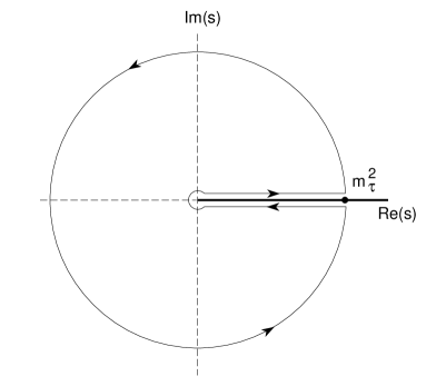
Figure 1: Integration contour in the complex $s$ plane, used to obtain Eq. (9)

The imaginary parts of the two–point functions $\,\Pi^{(J)}_{ij,V/A}(q^{2})\,$ are proportional to the spectral functions for hadrons with the corresponding quantum numbers. The semihadronic decay rate of the $\tau$ can be written as an integral of these spectral functions over the invariant mass $s$ of the final–state hadrons:

$$R_{\tau}=12\pi\int^{M_{\tau}^{2}}_{0}{ds\over M_{\tau}^{2}}\,\left(1-{s\over M_{\tau}^{2}}\right)^{2}\biggl{[}\left(1+2{s\over M_{\tau}^{2}}\right)\mbox{\rm Im}\Pi^{(1)}(s)+\mbox{\rm Im}\Pi^{(0)}(s)\biggr{]}.$$ (7)

The appropriate combinations of correlators are

$$\Pi^{(J)}(s)\equiv|V_{ud}|^{2}\,\left(\Pi^{(J)}_{ud,V}(s)+\Pi^{(J)}_{ud,A}(s)\right)+|V_{us}|^{2}\,\left(\Pi^{(J)}_{us,V}(s)+\Pi^{(J)}_{us,A}(s)\right).$$ (8)

The contributions coming from the first two terms correspond to $R_{\tau,V}$ and $R_{\tau,A}$ respectively, while $R_{\tau,S}$ contains the remaining Cabibbo–suppressed contributions.

Since the hadronic spectral functions are sensitive to the non-perturbative effects of QCD that bind quarks into hadrons, the integrand in Eq. (7) cannot be calculated at present from QCD. Nevertheless the integral itself can be calculated systematically by exploiting the analytic properties of the correlators $\Pi^{(J)}(s)$. They are analytic functions of $s$ except along the positive real $s$ axis, where their imaginary parts have discontinuities. The integral (7) can therefore be expressed as a contour integral in the complex $s$ plane running counter–clockwise around the circle $|s|=M_{\tau}^{2}$:

$$R_{\tau}=6\pi i\oint_{|s|=M_{\tau}^{2}}{ds\over M_{\tau}^{2}}\,\left(1-{s\over M_{\tau}^{2}}\right)^{2}\left[\left(1+2{s\over M_{\tau}^{2}}\right)\Pi^{(0+1)}(s)-2{s\over M_{\tau}^{2}}\Pi^{(0)}(s)\right].$$ (9)

The advantage of expression (9) over (7) is that it requires the correlators only for complex $s$ of order $M_{\tau}^{2}$, which is significantly larger than the scale associated with non-perturbative effects in QCD. The short–distance Operator Product Expansion (OPE) can therefore be used to organize the perturbative and non-perturbative contributions to the correlators into a systematic expansion $\!{}^{{\bf?}}$ in powers of $1/s$,

$$\Pi^{(J)}(s)=\sum_{D=2n}\,\sum_{\mbox{\rm\scriptsize dim}{\cal O}=D}{{\cal C}^{(J)}(s,\mu)\,\langle{\cal O}(\mu)\rangle\over(-s)^{D/2}},$$ (10)

where the inner sum is over local gauge–invariant scalar operators of dimension $D=0,2,4,\ldots$ The possible uncertainties associated with the use of the OPE near the time–like axis are absent in this case, because the integrand in Eq. (9) includes a factor $(1-s/M_{\tau}^{2})^{2}$, which provides a double zero at $s=M_{\tau}^{2}$, effectively suppressing the contribution from the region near the branch cut. The parameter $\mu$ in Eq. (10) is an arbitrary factorization scale, which separates long–distance non-perturbative effects, which are absorbed into the vacuum matrix elements $\langle{\cal O}(\mu)\rangle$, from short–distance effects, which belong in the Wilson coefficients ${\cal C}^{(J)}(s,\mu)$. The $D=0$ term (unit operator) corresponds to the pure perturbative contributions, neglecting quark masses. The leading quark–mass corrections generate the $D=2$ term. The first dynamical operators involving non-perturbative physics appear at $D=4$. Inserting the functions (10) into (9) and evaluating the contour integral, $R_{\tau}$ can be expressed as an expansion in powers of $1/M_{\tau}^{2}$, with coefficients that depend only logarithmically on $M_{\tau}$.

It is convenient to express the corrections to $R_{\tau}$ from dimension–$D$ operators in terms of the fractional corrections $\delta^{(D)}_{ij,V/A}$ to the naïve contribution from the current with quantum numbers $ij,V$ or $ij,A$:

$$R_{\tau,V/A} \!\!\!= \!\!\!{3\over 2}|V_{ud}|^{2}S_{EW}\left(1+\delta_{EW}^{\prime}+\sum_{D=2n}\delta^{(D)}_{ud,V/A}\right),$$

$$R_{\tau,S} \!\!\!= \!\!\!3\,|V_{us}|^{2}S_{EW}\left(1+\delta_{EW}^{\prime}+\sum_{D=2n}\delta^{(D)}_{us}\right).$$ (11)

$\delta^{(D)}_{ij}=(\delta^{(D)}_{ij,V}+\delta^{(D)}_{ij,A})/2$ is the average of the vector and axial–vector corrections. The dimension–0 contribution is the purely perturbative correction neglecting quark masses, which is the same for all the components of $R_{\tau}$: $\delta^{(0)}_{ij,V/A}=\delta^{(0)}$. The factors $\!{}^{{\bf?}}$

$$S_{EW}=\left({\alpha(m_{b}^{2})\over\alpha(M_{\tau}^{2})}\right)^{9\over 19}\left({\alpha(M_{W}^{2})\over\alpha(m_{b}^{2})}\right)^{9\over 20}\left({\alpha(M_{Z}^{2})\over\alpha(M_{W}^{2})}\right)^{36\over 17}=1.0194$$ (12)

and $\!{}^{{\bf?}}$

$$\delta_{EW}^{\prime}={5\over 12}\,{\alpha(M_{\tau}^{2})\over\pi}\simeq 0.0010\,,$$ (13)

contain the known electroweak corrections.

Adding the three terms, the total ratio $R_{\tau}$ is

$$R_{\tau}=3\left(|V_{ud}|^{2}+|V_{us}|^{2}\right)S_{EW}\biggl{\{}1+\delta_{EW}^{\prime}+\delta^{(0)}$$ (14)

$$\qquad\qquad\qquad\qquad\mbox{}+\sum_{D=2,4,...}\left(\cos^{2}\theta_{C}\delta^{(D)}_{ud}+\sin^{2}\theta_{C}\delta^{(D)}_{us}\right)\biggr{\}},$$

where $\sin^{2}\theta_{C}\equiv|V_{us}|^{2}/(|V_{ud}|^{2}+|V_{us}|^{2})$.

3 Perturbative Corrections

In the chiral limit ($m_{u}=m_{d}=m_{s}=0$), the vector and axial–vector currents are conserved. This implies $s\Pi^{(0)}(s)=0$; therefore, only the correlator $\Pi^{(0+1)}(s)$ contributes to Eq. (9). Owing $\!{}^{{\bf?},{\bf?}}$ to the chiral invariance of massless QCD, $\Pi^{(0+1)}_{ij,V}(s)=\Pi^{(0+1)}_{ij,A}(s)\equiv\Pi(s)$ ($i\not=j$) at any finite order in $\alpha_{s}$.

The result is more conveniently expressed in terms of the logarithmic derivative of the two–point correlation function of the vector (axial) current,

$$D(s)\equiv-s{d\over ds}\Pi(s)={1\over 4\pi^{2}}\sum_{n=0}K_{n}\left({\alpha_{s}(s)\over\pi}\right)^{n},$$ (15)

which satisfies an homogeneous renormalization–group equation. The $K_{n}$ coefficients are known $\!{}^{{\bf?},{\bf?},{\bf?},{\bf?},{\bf?}}$ to order $\alpha_{s}^{3}$. For $n_{f}=3$ quark flavours, one has:

$$K_{0}=K_{1}=1\,,$$

$$K_{2}={299\over 24}-9\zeta(3)=1.63982\,,$$ (16)

$$K_{3}(\overline{MS})={58057\over 288}-{779\over 4}\zeta(3)+{75\over 2}\zeta(5)=6.37101\,.$$

The perturbative component of $R_{\tau}$ is given by

$${R_{\tau}^{\mbox{\rm\scriptsize pert}}\over(|V_{ud}|^{2}+|V_{us}|^{2})S_{EW}}\equiv 3\,\{1+\delta^{(0)}\}=3\sum_{n=0}K_{n}\,A^{(n)}(\alpha_{s})\,,$$ (17)

where the functions $\!{}^{{\bf?}}$

$$A^{(n)}(\alpha_{s})={1\over 2\pi i}\oint_{|s|=M_{\tau}^{2}}{ds\over s}\,\left({\alpha_{s}(-s)\over\pi}\right)^{n}\left(1-2{s\over M_{\tau}^{2}}+2{s^{3}\over M_{\tau}^{6}}-{s^{4}\over M_{\tau}^{8}}\right)$$ (18)

are contour integrals in the complex plane, which only depend on $\alpha_{s}(M_{\tau}^{2})$.

The running coupling $\alpha_{s}(-s)$ in Eq. (18) can be expanded in powers of $\alpha_{s}(M_{\tau}^{2})$, with coefficients that are polynomials in $\log{(-s/M_{\tau}^{2})}$. The perturbative expansion of $\delta^{(0)}$ in powers of $a_{\tau}\equiv\alpha_{s}(M_{\tau}^{2})/\pi$ then takes the form $\!{}^{{\bf?},{\bf?},{\bf?},{\bf?},{\bf?},{\bf?},{\bf?}}$:

$$\delta^{(0)} \!\!\!= \!\!\!\sum_{n=1}(K_{n}+g_{n})\,a_{\tau}^{n},$$

$$\!\!\!= \!\!\!a_{\tau}+\left(K_{2}-{19\over 24}\beta_{1}\right)a_{\tau}^{2}$$

$$\!\!\!+\left(K_{3}-{19\over 12}K_{2}\beta_{1}-{19\over 24}\beta_{2}+{265-24\pi^{2}\over 288}\beta_{1}^{2}\right)a_{\tau}^{3}+\,{\cal O}(a_{\tau}^{4})$$

$$\!\!\!= \!\!\!a_{\tau}+5.2023\,a_{\tau}^{2}+26.366\,a_{\tau}^{3}+\,{\cal O}(a_{\tau}^{4})\,.$$

The complex integration along the circle $|s|=M_{\tau}^{2}$ generates the $g_{n}$ coefficients, which depend on $K_{m<n}$ and on $\beta_{m<n}$, where

$$\beta_{1}=-9/2\,,\qquad\beta_{2}=-8\,,\qquad\beta_{3}(\overline{MS})=-3863/192\,,\qquad\ldots$$ (20)

are the coefficients of the QCD $\beta$ function for $n_{f}=3$. One observes $\!{}^{{\bf?}}$ that the $g_{n}$ contributions are larger than the original $K_{n}$ coefficients ($g_{2}=3.5625$, $g_{3}=19.9949$). For instance, the bold–guess value $K_{4}\sim K_{3}(K_{3}/K_{2})\approx 25$ is to be compared with $g_{4}=78.0029$. These large corrections give rise to a sizeable renormalization scale dependence $\!{}^{{\bf?},{\bf?}}$ of the truncated ${\cal O}(a_{\tau}^{3})$ result. The reason of such uncomfortably large contributions $\!{}^{{\bf?}}$ stems from the long running along the circle $s=M_{\tau}^{2}\exp{(i\phi)}$ ($\phi\epsilon[0,2\pi]$) in Eq. (18). When the running coupling $\alpha_{s}(-s)$ is expanded in powers of $\alpha_{s}(M_{\tau}^{2})$, one gets imaginary logarithms, $\log{(-s/M_{\tau}^{2})}=i(\phi-\pi)$, which are large in some parts of the integration range. The radius of convergence of this expansion is actually quite small. A numerical analysis of the series $\!{}^{{\bf?}}$ shows that, at the three–loop level, an upper estimate for the convergence radius is $a_{\tau,\mbox{\rm\scriptsize conv}}\,<0.11$.

Note, however, that there is no deep reason to stop the $A^{(n)}(\alpha_{s})$ integral expansions at ${\cal O}(\alpha_{s}^{3})$. One can calculate the $A^{(n)}(\alpha_{s})$ expansion to all orders in $\alpha_{s}$, apart from the unknown $\beta_{n>3}$ contributions, which are likely to be negligible. Even for $a_{\tau}$ larger than the radius of convergence $a_{\tau,\mbox{\rm\scriptsize conv}}$, the integrals $A^{(n)}(\alpha_{s})$ are well–defined functions that can be numerically computed, by using in Eq. (18) the exact solution for $\alpha_{s}(-s)$ obtained from the renormalization–group $\beta$–function equation. Thus a more appropriate approach $\!{}^{{\bf?},{\bf?}}$ is to use a $K_{n}$ expansion of $R_{\tau}^{\mbox{\rm\scriptsize pert}}$ as in Eq. (17), and to fully keep the known three–loop calculation of the functions $A^{(n)}(\alpha_{s})$. The perturbative uncertainties are then reduced to the corrections coming from the unknown $\beta_{n>3}$ and $K_{n>3}$ contributions, since the $g_{n}$ contributions are properly resummed to all orders. To appreciate the size of the effect, Table 1 gives the exact results $\!{}^{{\bf?}}$ for $A^{(n)}(\alpha_{s})$ ($n=1,2,3$) obtained at the one–, two– and three–loop approximations (i.e. $\beta_{n>1}=0$, $\beta_{n>2}=0$, and $\beta_{n>3}=0$, respectively), together with the final value of $\delta^{(0)}$, for $a_{\tau}=0.1$. For comparison, the numbers coming from the truncated expressions at order $a_{\tau}^{3}$ are also given. Although the difference between the exact and truncated results represents a tiny $0.7\%$ effect on $R_{\tau}$, it produces a sizeable $4\%$ shift on the value of $\delta^{(0)}$. The $\delta^{(0)}$ shift, which reflects into a corresponding shift in the experimental $\alpha_{s}(M_{\tau}^{2})$ determination, depends strongly on the value of the coupling constant; for $a_{\tau}=0.14$ the $\delta^{(0)}$ shift reaches the $-20\%$ level.

Table 1: Exact results for $A^{(n)}(\alpha_{s})$ ($n=1,2,3$) obtained at the one– ($\beta_{n>1}=0$), two– ($\beta_{n>2}=0$) and three–loop ($\beta_{n>3}=0$) approximations, together with the final value of $\delta^{(0)}$, for $a_{\tau}=0.1$. For comparison, the numbers coming from the truncated expressions at order $a_{\tau}^{3}$ are also given.

Loops	$A^{(1)}$	$A^{(2)}$	$A^{(3)}$	$\delta^{(0)}$
$1$	$0.13247$	$0.01570$	$0.00170$	$0.1690$
$2$	$0.13523$	$0.01575$	$0.00163$	$0.1714$
$3$	$0.13540$	$0.01565$	$0.00160$	$0.1712$
${\cal O}(\alpha_{s}^{3})$	$0.14394$	$0.01713$	$0.00100$	$0.1784$

Notice that the difference between using the one– or two–loop approximation to the $\beta$ function is already quite small ($1.4\%$ effect on $\delta^{(0)}$), while the change induced by the three–loop corrections is completely negligible ($0.1\%$). Therefore (unless the $\beta$ function has some unexpected pathological behaviour at higher orders), the error induced by the truncation of the $\beta$ function at third order should be smaller than $0.1\%$ and therefore can be safely neglected. The sensitivity on the choice of renormalization scale and renormalization scheme is also very small $\!{}^{{\bf?},{\bf?}}$.

Table 2: $\delta^{(0)}$ for different values of $\alpha_{s}(M_{\tau}^{2})$.

$\alpha_{s}(M_{\tau}^{2})$	$\delta^{(0)}$		$\Delta(\delta^{(0)})$
	$K_{4}=0$	$K_{4}=27.5$
$0.30$	$0.161$	$0.164$	$\pm 0.006$
$0.31$	$0.168$	$0.172$	$\pm 0.007$
$0.32$	$0.176$	$0.180$	$\pm 0.008$
$0.33$	$0.183$	$0.188$	$\pm 0.008$
$0.34$	$0.191$	$0.196$	$\pm 0.009$
$0.35$	$0.198$	$0.203$	$\pm 0.010$
$0.36$	$0.205$	$0.211$	$\pm 0.010$
$0.37$	$0.213$	$0.219$	$\pm 0.011$
$0.38$	$0.220$	$0.226$	$\pm 0.012$
$0.39$	$0.227$	$0.234$	$\pm 0.012$
$0.40$	$0.234$	$0.241$	$\pm 0.013$

The dominant perturbative uncertainties come from the unknown higher–order coefficients $K_{n>3}$. The ${\cal O}(\alpha_{s}^{4})$ contribution has been estimated $\!{}^{{\bf?}}$ using scheme–invariant methods, namely the principle of minimal sensitivity $\!{}^{{\bf?}}$ and the effective charge approach $\!{}^{{\bf?}}$, with the result $\!{}^{{\bf?}}$:

$$K_{4}^{\mbox{\rm\scriptsize est}}=27.5\,.$$ (21)

This number is very close to the naïve guess $\!{}^{{\bf?}}$ $K_{4}\sim(K_{3}/K_{2})K_{3}\approx 25$. A similar estimate, $K_{4}^{\mbox{\rm\scriptsize NNA}}=24.8$, is obtained $\!{}^{{\bf?},{\bf?},{\bf?},{\bf?},{\bf?},{\bf?},{\bf?}}$ in the limit of a large number of quark flavours, using the so–called naive non-abelianization prescription $\!{}^{{\bf?}}$ ($n_{f}\to 3\beta_{1}=n_{f}-{33\over 2}=-{27\over 2}$). From a fit to the experimental $\tau$ data, the value $K_{4}^{\mbox{\rm\scriptsize fit}}=29\pm 5$ has been also quoted $\!{}^{{\bf?}}$.

Using the estimate (21), the ${\cal O}(\alpha_{s}^{4})$ correction amounts to a 0.004 increase of $\delta^{(0)}$ for $a_{\tau}=0.1$. The resulting perturbative contribution $\delta^{(0)}$, obtained through Eqs. (17) and (18), is given in Table 2 for different values of the strong coupling constant $\alpha_{s}(M_{\tau}^{2})$. In order to be conservative, and to account for all possible sources of perturbative uncertainties, we have used $\!{}^{{\bf?},{\bf?}}$

$$\Delta(\delta^{(0)})=\pm 50\,A^{(4)}(\alpha_{s})\,,$$ (22)

as an estimate of the theoretical error on $\delta^{(0)}$. Note that, for the relevant values of $\alpha_{s}$, this is of the same size as $K_{3}\,A^{(3)}(\alpha_{s})$; thus, this error estimate is conservative enough to apply $\!{}^{{\bf?}}$ in the worst possible scenario, where the onset of the asymptotic behaviour of the perturbative series were already reached for $n=3,4$.

There have been attempts $\!{}^{{\bf?},{\bf?},{\bf?},{\bf?},{\bf?}}$ to improve the perturbative prediction by performing an all–order summation a certain class of higher–order corrections (the so-called ultraviolet renormalon chains). This can be accomplished using exact large–$n_{f}$ results and applying the naive non-abelianization prescription $\!{}^{{\bf?}}$. Unfortunately, the naive resummation turns out to be renormalization–scheme dependent beyond one loop $\!{}^{{\bf?},{\bf?}}$. More recently, a renormalization–scheme–invariant summation has been presented $\!{}^{{\bf?}}$. The final effect of the higher–order corrections (beyond $K_{4}$) turns out to be small.

4 Power Corrections

The $1/M_{\tau}^{2}$ contributions $\delta^{(2)}_{ij}$ to the ratio $R_{\tau}$ are simply the leading quark–mass corrections to the perturbative QCD result of the previous section. These contributions are known $\!{}^{{\bf?},{\bf?}}$ to order $\alpha_{s}^{2}$. Quark–mass corrections are certainly tiny for the up and down quarks ($\delta^{(2)}_{ud}\sim-0.08\%$), but the correction from the strange–quark mass is important for strange decays $\!{}^{{\bf?},{\bf?}}$: ($m_{u}=m_{d}=0$)

$$\delta^{(2)}_{us,V/A}=-8{\overline{m}_{s}^{2}\over M_{\tau}^{2}}\left\{1+{16\over 3}a_{\tau}+11.03\,a_{\tau}^{2}\right\},$$ (23)

where $\overline{m}_{s}\equiv m_{s}(M_{\tau}^{2})$ is the running mass of the strange quark evaluated at the scale $M_{\tau}$. For $\alpha_{s}(M_{\tau}^{2})=0.35$, $\delta^{(2)}_{us}\approx-20\%$; nevertheless, because of the $\sin^{2}{\theta_{C}}$ suppression, the effect on the total ratio $R_{\tau}$ is only $-(1.0\pm 0.2)\%$.

Since the $\tau$ mass is a quite low energy scale, we should worry about possible non-perturbative effects. In the framework of the OPE, the long–distance dynamics is absorbed into the vacuum matrix elements $\langle{\cal O}(\mu)\rangle$, which are (at present) quantities to be fixed phenomenologically. If the logarithmic dependence of the Wilson coefficients ${\cal C}^{(J)}(s,\mu)$ on $s$ is neglected (this is an effect of order $\alpha_{s}^{2}$), the contour integrals can be evaluated trivially using Cauchy’s residue theorem, and are non-zero only for $D=2,4,6$ and $8$. The corrections simplify even further if we also take the chiral limit ($m_{u}=m_{d}=m_{s}=0$). The dimension–2 corrections then vanish because there are no operators of dimension 2. In the chiral limit, $s\Pi^{(0)}(s)=0$; thus only the $\Pi^{(0+1)}(s)$ term in Eq. (9) contributes to $R_{\tau}$. The form of the kinematical factor multiplying $\Pi^{(0+1)}(s)$ in Eq. (9) is such that, when the $s$–dependence of the Wilson coefficients is ignored, only the $D=6$ and $D=8$ contributions survive the integration. The power corrections to $R_{\tau}$ then reduce to $\!{}^{{\bf?},{\bf?},{\bf?},{\bf?}}$

$$\delta^{(6)}_{ij,V/A} \!\!\!\simeq \!\!\!-24\pi^{2}{\left[\sum{\cal C}^{(0+1)}_{ij,V/A}\langle{\cal O}\rangle\right]^{(D=6)}\over M_{\tau}^{6}}\,,$$

$$\delta^{(8)}_{ij,V/A} \!\!\!\simeq \!\!\!-16\pi^{2}{\left[\sum{\cal C}^{(0+1)}_{ij,V/A}\langle{\cal O}\rangle\right]^{(D=8)}\over M_{\tau}^{8}}\,,$$ (24)

and $\delta^{(2n)}_{ij,V/A}\simeq 0$ for $2n\not=6,8$.

When the logarithmic dependence of the Wilson coefficients on $s$ is taken into account, operators of dimensions other than 6 and 8 do contribute, but they are suppressed by two powers of $\alpha_{s}(M_{\tau}^{2})$. The largest power corrections to $R_{\tau}$ then come from dimension–6 operators, which have no such suppression. Their size was first estimated in Ref. 5, using published phenomenological fits to different sets of data:

$$\delta^{(6)}_{ij}\approx-{2\over 7}\delta^{(6)}_{ij,V}\approx{2\over 11}\delta^{(6)}_{ij,A}\approx-(0.7\pm 0.4)\%.$$ (25)

These power corrections are numerically very small, which is due to the fact that they fall off like the sixth power of $1/M_{\tau}$. Moreover, there is a large cancellation between the vector and axial–vector contributions to the total hadronic width (the operator with the largest Wilson coefficient contributes with opposite signs to the vector and axial–vector correlators, due to the $\gamma_{5}$ flip). Thus, the non-perturbative corrections to $R_{\tau}$ are smaller than the corresponding contributions to $R_{\tau,V/A}$. A more detailed study of non-perturbative corrections, including the very small $D=4$ contributions proportional to quark masses or to $\alpha_{s}(M_{\tau}^{2})^{2}$, can be found in Ref. 5.

The estimate (25) introduces a small uncertainty in the $R_{\tau}$ predictions, since the actual evaluation of the non-perturbative contributions involves a mixture of experimental measurements and theoretical considerations, which are model–dependent to some extent. It is better to directly measure those contributions from the $\tau$–decay data themselves. This information can be extracted $\!{}^{{\bf?}}$ from the invariant–mass distribution of the final hadrons in $\tau$ decay.

Although the distributions themselves cannot be predicted at present, certain weighted integrals of the hadronic spectral functions can be calculated in the same way as $R_{\tau}$. The analyticity properties of $\Pi^{(J)}_{ij,V/A}$ imply $\!{}^{{\bf?},{\bf?}}$:

$$\int_{0}^{s_{0}}ds\,W(s)\>\mbox{\rm Im}\Pi^{(J)}_{ij,V/A}\,=\,{i\over 2}\oint_{|s|=s_{0}}ds\,W(s)\,\Pi^{(J)}_{ij,V/A}\,,$$ (26)

with $W(s)$ an arbitrary weight function without singularities in the region $|s|\leq s_{0}$. Generally speaking, the accuracy of the theoretical predictions can be much worse than the one of $R_{\tau}$, because non-perturbative effects are not necessarily suppressed. In fact, choosing an appropriate weight function, non-perturbative effects can even be made to dominate the final result. But this is precisely what makes these integrals interesting: they can be used to measure the parameters characterizing the non-perturbative dynamics.

To perform an experimental analysis, it is convenient to use moments of the directly measured invariant–mass distribution $\!{}^{{\bf?}}$ ($k,l\geq 0$)

$$R^{kl}_{\tau}(s_{0})\equiv\int_{0}^{s_{0}}\,ds\,\left(1-{s\over s_{0}}\right)^{k}\left({s\over M_{\tau}^{2}}\right)^{l}{dR_{\tau}\over ds}\,.$$ (27)

The factor $(1-s/s_{0})^{k}$ supplements $(1-s/M_{\tau}^{2})^{2}$ for $s_{0}\not=M_{\tau}^{2}$, in order to squeeze the integrand at the crossing of the positive real axis and, therefore, improves the reliability of the OPE analysis; moreover, for $s_{0}=M_{\tau}^{2}$ it reduces the contribution from the tail of the distribution, which is badly defined experimentally. A combined fit of different $R_{\tau}^{kl}(s_{0})$ moments results in experimental values for $\alpha_{s}(M_{\tau}^{2})$ and for the coefficients of the inverse power corrections in the OPE. $R_{\tau}^{00}(M_{\tau}^{2})=R_{\tau}$ uses the overall normalization of the hadronic distribution, while the ratios $D_{\tau}^{kl}(M_{\tau}^{2})=R^{kl}_{\tau}(M_{\tau}^{2})/R_{\tau}$ are based on the shape of the $s$ distribution and are more dependent on non-perturbative effects $\!{}^{{\bf?}}$.

The predicted suppression $\!{}^{{\bf?},{\bf?},{\bf?},{\bf?}}$ of the non-perturbative corrections has been confirmed by ALEPH $\!{}^{{\bf?},{\bf?}}$ and CLEO $\!{}^{{\bf?}}$, using the moments (0,0), (1,0), (1,1), (1,2) and (1,3). The most recent ALEPH analysis $\!{}^{{\bf?}}$ gives:

$$\delta_{\mbox{\rm\scriptsize NP}}\equiv\sum_{D\geq 4}\left(\cos^{2}\theta_{C}\delta^{(D)}_{ud}+\sin^{2}\theta_{C}\delta^{(D)}_{us}\right)=-(0.5\pm 0.7)\%\,,$$ (28)

in agreement with (25).

5 Phenomenology

The QCD prediction for $R_{\tau}$ is then completely dominated by the perturbative contribution $\delta^{(0)}$; non-perturbative effects being of the order of the perturbative uncertainties from uncalculated higher–order corrections $\!{}^{{\bf?},{\bf?},{\bf?}}$. Furthermore, as shown in Table 2, the result turns out to be very sensitive to the value of $\alpha_{s}(M_{\tau}^{2})$, allowing for an accurate determination of the fundamental QCD coupling.

The experimental value for $R_{\tau}$ can be obtained from the leptonic branching fractions or from the $\tau$ lifetime. The average of those determinations $\!{}^{{\bf?}}$

$$R_{\tau}=3.649\pm 0.014\,,$$ (29)

corresponds to

$$\alpha_{s}(M_{\tau}^{2})=0.355\pm 0.025\,.$$ (30)

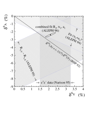
Figure 2: Constraints on $\delta^{(6)}_{V}$ and $\delta^{(6)}_{A}$ obtained from ALEPH data $\!{}^{{\bf?}}$. The ellipse depicts the combined fit. All results are still preliminary. (Taken from Ref. 45)

Once the running coupling constant $\alpha_{s}(s)$ is determined at the scale $M_{\tau}$, it can be evolved to higher energies using the renormalization group. The size of its error bar scales roughly as $\alpha_{s}^{2}$, and it therefore shrinks as the scale increases. Thus a modest precision in the determination of $\alpha_{s}$ at low energies results in a very high precision in the coupling constant at high energies. After evolution up to the scale $M_{Z}$, the strong coupling constant in (30) decreases to

$$\alpha_{s}(M_{Z}^{2})=0.1225\pm 0.0025\,,$$ (31)

in excellent agreement with the direct measurement $\!{}^{{\bf?},{\bf?}}$ at $\mu=M_{Z}$, $\alpha_{s}(M_{Z}^{2})=0.121\pm 0.003$, and with a similar error bar. The comparison of these two determinations of $\alpha_{s}$ in two extreme energy regimes, $M_{\tau}$ and $M_{Z}$, provides a beautiful test of the predicted running of the QCD coupling.

With $\alpha_{s}(M_{\tau}^{2})$ fixed to the value in Eq. (30), the same theoretical framework gives definite predictions $\!{}^{{\bf?},{\bf?}}$ for the semi-inclusive $\tau$ decay widths $R_{\tau,V}$, $R_{\tau,A}$ and $R_{\tau,S}$, in good agreement with the experimental measurements $\!{}^{{\bf?},{\bf?}}$. The separate analysis of the vector and axial–vector contributions allows to investigate the associated non-perturbative corrections ($R_{\tau,V}-R_{\tau,A}$ is a pure non-perturbative quantity). Figure 2 shows $\!{}^{{\bf?}}$ the (preliminary) constraints on $\delta^{(6)}_{V}$ and $\delta^{(6)}_{A}$ obtained from the most recent ALEPH analyses $\!{}^{{\bf?},{\bf?},{\bf?}}$. A clear improvement over previous phenomenological determinations $\!{}^{{\bf?},{\bf?}}$ is apparent.

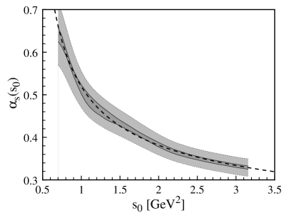
Figure 3: Values of $\alpha_{s}(s_{0})$ extracted $\!{}^{{\bf?}}$ from the $R_{\tau}^{00}(s_{0})$ data $\!{}^{{\bf?},{\bf?}}$. The dashed line shows the three–loop QCD prediction for the running coupling constant. (Taken from Ref. 51)

The Cabibbo–suppressed width $R_{\tau,S}$ is very sensitive to the value of the strange quark mass $\!{}^{{\bf?}}$, providing a direct and clean way of measuring $m_{s}$. A very preliminary value, $m_{s}(M_{\tau}^{2})=(212\,{}^{+30\,+1}_{-35\,-5})$ MeV, has been already presented at the last tau workshop $\!{}^{{\bf?}}$.

Using the measured invariant–mass distribution of the final hadrons, it is possible to evaluate the integral $R_{\tau}^{00}(s_{0})$, with an arbitrary upper limit of integration $s_{0}\leq M_{\tau}^{2}$. The experimental $s_{0}$ dependence agrees well with the theoretical predictions $\!{}^{{\bf?}}$ up to rather low values$\!{}^{{\bf?}}$ of $s_{0}$ ($>0.7$ GeV²). Equivalently, from the measured $\!{}^{{\bf?},{\bf?}}$ $R_{\tau}^{00}(s_{0})$ distribution one obtains $\alpha_{s}(s_{0})$ as a function of the scale $s_{0}$. As shown $\!{}^{{\bf?}}$ in Figure 3, the result exhibits an impressive agreement with the running predicted at three–loop order by QCD. It is important to realize $\!{}^{{\bf?}}$ that the theoretical prediction for $R_{\tau}^{00}(s_{0})$ does not contain inverse powers of $s_{0}$ (as long as the $s$–dependence of the Wilson coefficients is ignored). The power corrections are suppressed by powers of $1/M_{\tau}^{2}$; thus, they do not drive a break–down of the OPE. This could explain the surprisingly good agreement with the data for $s_{0}~{}{}_{\textstyle\sim}^{\textstyle<}~{}1$ GeV²

A similar test was performed before $\!{}^{{\bf?}}$ for $R_{\tau,V}$, using the vector spectral function measured in $e^{+}e^{-}\to$ hadrons, and varying the value of the tau mass. This allows to study the behaviour of the OPE at lower scales. The theoretical predictions for $R_{\tau,V}$ as function of $M_{\tau}^{2}$ agree $\!{}^{{\bf?}}$ well with the data for $M_{\tau}>1.2$ GeV. Below this value, higher–order inverse power corrections become very important and eventually generate the expected break–down of the expansion in powers of $1/M_{\tau}^{2}$.

6 Summary

Because of its inclusive nature, the total hadronic width of the $\tau$ can be rigorously computed within QCD. One only needs to study two–point correlation functions for the vector and axial–vector currents. As shown in Eq. (9), this information is only needed in the complex plane, away from the time–like axis; the dangerous region near the physical cut does not contribute at all to the result, because of the phase–space factor $(1-s/M_{\tau}^{2})^{2}$. The uncertainties of the theoretical predictions are then quite small.

The ratio $R_{\tau}$ is very sensitive to the value of the strong coupling, and therefore can be used $\!{}^{{\bf?}}$ to measure $\alpha_{s}(M_{\tau}^{2})$. This observation has triggered an ongoing effort to improve the knowledge of $R_{\tau}$ from both the experimental and the theoretical sides. The fact that $M_{\tau}$ is a quite low energy scale (i.e. that $\alpha_{s}(M_{\tau}^{2})$ is big), but still large enough to allow a perturbative analysis, makes $R_{\tau}$ an ideal observable to determine the QCD coupling. Moreover, since the error of $\alpha_{s}(\mu^{2})$ shrinks as $\mu$ increases, the good accuracy of the $R_{\tau}$ determination of $\alpha_{s}(M_{\tau}^{2})$ implies a very precise value of $\alpha_{s}(M_{Z}^{2})$.

The theoretical analysis of $R_{\tau}$ has reached a very mature level. Many different sources of possible perturbative and non-perturbative contributions have been analyzed in detail. A very detailed study of the associated uncertainties has been given in Ref. 8. The final theoretical uncertainty is small and has been adequately taken into account in the final $\alpha_{s}(M_{\tau}^{2})$ determination in Eq. (30).

The comparison of the theoretical predictions with the experimental data shows a successful and consistent picture. The $\alpha_{s}(M_{\tau}^{2})$ determination is in excellent agreement with the measurements at the $Z$–mass scale, providing clear evidence of the running of $\alpha_{s}$. Moreover, the analysis of the semi-inclusive components of the $\tau$ hadronic width, $R_{\tau,V}$, $R_{\tau,A}$ and $R_{\tau,S}$, and the invariant–mass distribution of the final decay products gives a further confirmation of the reliability of the theoretical framework, and allows to investigate other important QCD parameters such as the strange–quark mass or the non-perturbative vacuum condensates.

References

References

• [1]
• [2] E. Braaten, Phys. Rev. Lett. 60 (1988) 1606; Phys. Rev. D39 (1989) 1458.
• [3] S. Narison and A. Pich, Phys. Lett. B211 (1988) 183.
• [4] A. Pich, Hadronic Tau-Decays and QCD, Proc. Workshop on Tau Lepton Physics (Orsay, 1990), eds. M. Davier and B. Jean-Marie (Ed. Frontières, Gif-sur-Yvette, 1991), p. 321.
• [5] E. Braaten, S. Narison and A. Pich, Nucl. Phys. B373 (1992) 581.
• [6] F. Le Diberder and A. Pich, Phys. Lett. B286 (1992) 147.
• [7] A. Pich, QCD Predictions for the Tau Hadronic Width and Determination of $\alpha_{s}(m_{\tau}^{2})$, Proc. Second Workshop on Tau Lepton Physics (Ohio, 1992), ed. K.K. Gan (World Scientific, Singapore, 1993), p. 121.
• [8] A. Pich, Nucl. Phys. B (Proc. Suppl.) 39B,C (1995) 326.
• [9] S. Narison, Nucl. Phys. B (Proc. Suppl.) 40 (1995) 47.
• [10] E. Braaten, Perturbative QCD and Tau Decay, Proc. Fourth Workshop on Tau Lepton Physics –TAU96– (Colorado, 16–19 September 1996), ed. J. Smith, Nucl. Phys. B (Proc. Suppl.) in press.
• [11] A. Pich, Tau Lepton Physics: Theory Overview, Proc. Fourth Workshop on Tau Lepton Physics –TAU96– (Colorado, 16–19 September 1996), ed. J. Smith, Nucl. Phys. B (Proc. Suppl.) in press [IFIC/96-96; hep-ph/9612308].
• [12] M.A. Shifman, A.L. Vainshtein and V.I. Zakharov, Nucl. Phys. B147 (1979) 385; 448; 519.
• [13] W.J. Marciano and A. Sirlin, Phys. Rev. Lett. 61 (1988) 1815; 56 (1986) 22.
• [14] E. Braaten and C.S. Li, Phys. Rev. D42 (1990) 3888.
• [15] T.L. Trueman, Phys. Lett. 88B (1979) 331.
• [16] A.I. Antoniadis, Phys. Lett. 84B (1979) 223.
• [17] K.G. Chetyrkin, A.L. Kataev and F.V. Tkachov, Phys. Lett. 85B (1979) 277.
• [18] M. Dine and J. Sapirstein, Phys. Rev. Lett. 43 (1979) 668.
• [19] W. Celmaster and R. Gonsalves, Phys. Rev. Lett. 44 (1980) 560.
• [20] S.G. Gorishny, A.L. Kataev and S.A. Larin, Phys. Lett. B259 (1991) 144.
• [21] L.R. Surguladze and M.A. Samuel, Phys. Rev. Lett. 66 (1991) 560.
• [22] J. Chýla, A. Kataev and S. Larin, Phys. Lett. B267 (1991) 269.
• [23] A.A. Pivovarov, Z. Phys. C53 (1992) 461.
• [24] P.A. Raczka and A. Szymacha, Z. Phys. C70 (1996) 125.
• [25] A.L. Kataev and V.V. Starshenko, Mod. Phys. Lett. A10 (1995) 235.
• [26] P.M. Stevenson, Phys. Rev. D23 (1981) 2916.
• [27] G. Grunberg, Phys. Lett. B221 (1980) 70; Phys. Rev. D29 (1984) 2315.
• [28] D.J. Broadhurst, Z. Phys. C58 (1993) 339.
• [29] D.J. Broadhurst and A.L. Kataev, Phys. Lett. B315 (1993) 179.
• [30] M. Beneke, Nucl. Phys. B405 (1993) 424; Phys. Lett. B307 (1993) 154.
• [31] C.N. Lowett–Turner and C.G. Maxwell, Nucl. Phys. B452 (1995) 188;
432 (1994) 147.
• [32] M. Beneke and V.M. Braun, Phys. Lett. B348 (1995) 513.
• [33] P. Ball, M. Beneke and V.M. Braun, Nucl. Phys. B452 (1995) 563.
• [34] M. Neubert, Nucl. Phys. B463 (1996) 511.
• [35] D.J. Broadhurst and A.G. Grozin, Phys. Rev. D52 (1995) 4082.
• [36] F. Le Diberder, Nucl. Phys. B (Proc. Suppl.) 39B,C (1995) 318.
• [37] J. Chýla, Phys. Lett. B356 (1995) 341.
• [38] C.J. Maxwell and D.G. Tonge, RS–Invariant All–Orders Renormalon Resummations for some QCD Observables, [hep-ph/9606392].
• [39] K.G. Chetyrkin and A. Kwiatkowski, Z. Phys. C59 (1993) 525.
• [40] A. Pich, QCD Tests From Tau Decay Data, in Proc. Tau-Charm Factory Workshop (SLAC, 1989), ed. L.V. Beers, SLAC-Report-343 (1989), p. 416.
• [41] F. Le Diberder and A. Pich, Phys. Lett. B289 (1992) 165.
• [42] D. Buskulic et al (ALEPH), Phys. Lett. B307 (1993) 209.
• [43] L. Duflot, Nucl. Phys. B (Proc. Suppl.) 40 (1995) 37.
• [44] T. Coan et al (CLEO), Phys. Lett. B356 (1995) 580.
• [45] A. Höcker, Vector and Axial–Vector Spectral Functions and QCD, Proc. Fourth Workshop on Tau Lepton Physics –TAU96– (Colorado, 16–19 September 1996), ed. J. Smith, Nucl. Phys. B (Proc. Suppl.) in press.
• [46] D. Buskulic et al (ALEPH), Z. Phys. C70 (1996) 579.
• [47] M. Schmelling, Status of the Strong Coupling Constant, Proc. XXVIII Intern. Conf. on High Energy Physics (Warsaw, 25–31 July 1996) in press [hep-ex/9701002].
• [48] S. Bethke, Experimental Tests of Asymptotic Freedom, Proc. QCD’96 (Montpellier, 1996), ed. S. Narison [hep-ex/9609014].
• [49] M. Davier, $\tau$ Decays into Strange Particles and QCD, Proc. Fourth Workshop on Tau Lepton Physics –TAU96– (Colorado, 16–19 September 1996), ed. J. Smith, Nucl. Phys. B (Proc. Suppl.) in press.
• [50] S. Narison, Phys. Lett. B361 (1995) 121.
• [51] M. Girone and M. Neubert, Phys. Rev. Lett. 76 (1996) 3061.
• [52] S. Narison and A. Pich, Phys. Lett. B304 (1993) 359.