${\bf k}$-Factorization and Small-$x$ Anomalous Dimensions

Abstract

We investigate the consistency requirements of the next-to leading BFKL equation with the renormalization group, with particular emphasis on running coupling effects and NL anomalous dimensions. We show that, despite some model dependence of the bare hard Pomeron, such consistency holds at leading twist level, provided the effective variable $\alpha_{s}(t)\log(1/x)$ is not too large. We give a unified view of resummation formulas for coefficient functions and anomalous dimensions in the $Q_{0}$-scheme and we discuss in detail the new one for the $q\bar{q}$ contributions to the gluon channel.

PACS 12.38.Cy

1 Introduction

The understanding of small-$x$ scaling violations in QCD has become increasingly important with the discovery of the steep rise of structure functions at HERA[1]. Such rise may be related to the hard Pomeron[2] small-$x$ behaviour[3], but may be also understood through large scaling violations[4] and may also fit in a fixed order perturbative approach[5].

The above ambiguities are partly unavoidable, because of the lack of sufficiently precise [1], independent measurements of small-$x$ parton densities[6], but are partly due to the lack of complete understanding of scaling violations, at theoretical level. In fact, in the small-$x$ region, the QCD perturbative series is affected by large logarithms - similarly to what happens in semihard processes [7] - and becomes dependent on the effective coupling constant $\alpha_{s}(t)\log{1/x}$ or $\alpha_{s}(t)/\omega$, where $t\equiv\log(Q^{2}/\Lambda^{2})$ and $\omega=N-1$ is the moment index.

Therefore, a hierarchy of perturbative terms is defined in the usual way

$$\gamma(\alpha_{s},\omega)=\gamma_{L}\left(\frac{\alpha_{s}}{\omega}\right)+\alpha_{s}\gamma_{NL}\left(\frac{\alpha_{s}}{\omega}\right)+NNL-\text{terms}$$ (1.1)

for both the singlet anomalous dimension matrix and the coefficient functions. Furthermore, since gluons couple to electro-weak probes only through quarks, we actually need leading (L) coefficient functions and up to next-to-leading (NL) anomalous dimensions, in order to have a factorization scheme independent result for DIS.

This theoretical program has been partly achieved at quark level [8-10], but is not yet complete at gluon level, despite various efforts [11-14]. Nevertheless, such completion is needed in order to well understand scaling violations, and then be able to look at the small-$x$ behaviour of initial data[15] so as to find the hard Pomeron rise, if any.

In this paper we wish to present a resummation method which is valid for all the relevant quantities up to NL level, and to apply it to coefficients and anomalous dimensions in the so called $Q_{0}$-scheme [15], including the new $q\bar{q}$ contributions to the gluon anomalous dimension, already reported in a short note [16]. The method is based on the idea of ${\bf k}$-factorization [8, 9], which is just a way of exploiting the consistency of high-energy factorized quantities, which are ${\bf k}$-dependent, with Renormalization Group (R.G.) factorization, which is not. The all-order resummation is obtained by ${\bf k}$-integrations of low order ${\bf k}$-dependent kernels.

Therefore, we shall proceed in two steps. Our first goal is to explicitate the NL consistency requirements between high-energy and collinear factorization with running coupling referring, for definiteness, to hard processes of DIS type, characterized by a probe with a large scale $Q$ and by a target with scale $Q_{0}\ll Q$. This will allow us to obtain well defined resummation formulas in terms of kernels of BFKL type [2], up to NL level.

As a second step, we shall proceed to the study of the NL kernel itself, of its eigenvalues, and of the resummed formulas for the $q\bar{q}$ contributions. This study is based on the phase-space integration of the squared $Q\bar{Q}$ production matrix elements [8], combined with the virtual corrections available in the literature [13, 14].

To start illustrating the first step, let us notice that ${\bf k}$-factorization is due to the exchange of an off-shell gluon of virtuality $t\simeq-{\bf k}^{2}$, which behaves, at high energies, as a Regge pole yielding a quasi-constant cross-section. On the other hand, collinear factorization is due to nearly on-shell quarks and gluons, providing logarithmic scaling violations.

Therefore, the two kinds of factorization are not related a priori. In unbroken gauge theories like QCD, a relationship can be established because the (Regge) gluon polarization coincides, on shell, with one of the collinear polarizations [17]. For instance, at one loop level, Regge behaviour is established, in the gluon channel, by the singular behaviour of the DGLAP splitting functions [18]

$$P_{gg}(z)\simeq\frac{2C_{A}}{z},\quad\quad P_{gq}(z)\simeq\frac{2C_{F}}{z},$$ (1.2)

or in moment index space $\omega=N-1$, by a correspondingly singular anomalous dimension matrix

$$\gamma_{ab}=\frac{\bar{\alpha_{s}}}{\omega}\begin{pmatrix}0&0\\ \frac{C_{F}}{C_{A}}&1\end{pmatrix}+{\hat{\gamma}}_{ab}+O(\omega)$$ (1.3)

$$\left(a,b\>=\>q,g,~{}~{}~{}~{}~{}~{}~{}~{}~{}~{}~{}~{}~{}~{}~{}~{}~{}~{}~{}~{}~{}~{}~{}~{}\bar{\alpha_{s}}=\frac{\alpha_{s}C_{A}}{\pi}\right).$$

However, establishing such relationship at next to leading level requires the treatment of several subtle points. Firstly, ${\bf k}$-factorization is useful in the gluon channel only, while collinear factorization involves both gluons and quark-sea. How to recover from the former the two-channel picture of the latter?

Furthermore, even in the gluon channel, the high energy exchange does not yield all collinear singular gluon contributions, some of which occur at low energies, as is apparent from Eq. (1.3). How to relate the two gluon definitions and to get all subleading terms?

Finally, the renormalization group evolution with running coupling has been always assumed in order to extract physical predictions from ${\bf k}$-factorization. Is this behaviour really consistent with the BFKL equation and its ”hard Pomeron” singularity at NL level?

In Sec. 2 we shall show, on the basis of the work of Fadin, Lipatov and collaborators [11-14] and of our group [8-10,16], that a detailed comparison of high-energy and renormalization group is nevertheless possible and provides resummation formulas for the NL anomalous dimension matrix (and for the leading coefficient functions) in the $Q_{0}$ factorization scheme.

The basic point is that, as it appears from Refs. [8-16] and Ref. [19], $s$-channel iteration is not yet relevant at NL $\log s$ level, while $t$-channel iteration is provided by a generalized high energy integral equation, in which low energy ${\bf k}$-dependent kernels occur. This result, with some modifications, forms the basis for the representation of the two-scale problems with anomalous dimensions that we provide here.

Some of the questions asked above do have a tricky answer, however. Firstly, even at leading twist level, we find that the renormalization group representation with running coupling is valid, for $\omega\ll 1$, only in the regime of $t=\log\frac{Q^{2}}{\Lambda^{2}}\gg t_{0}>1$, with

$$b\omega t>c$$ (1.4)

where the critical constant $c$ is related to the BFKL kernel. This means that we have to stay away from a $t$-dependent singularity in the $\omega$ plane, or in other words, that the effective variable $\alpha_{s}(t)\log(1/x)$ should not be too large.

Furthermore, the bare hard Pomeron singularity, which occurs in the coefficient function, and ultimately dominates the small-$x$ behaviour, turns out to be dependent on the large distance behaviour of the running coupling, due to a diffusion process towards low values of ${\bf k}^{2}$. Fortunately, this fact does not affects the R. G. factorization, valid in the regime (1.4) [20].

Finally, within the anomalous dimension representation, the two-channel picture obtains because of the presence of two distinct anomalous dimension eigenvalues $\gamma_{+}$, $\gamma_{-}$, $\gamma_{+}$ being the leading one. While the NL hierarchy is straightforward for the $\gamma_{+}$ contributions, it requires careful handling of a whole chain of collinear singular kernels for the $\gamma_{-}$ contribution, as we shall see.

In other words, comparing the high-energy and R. G. approaches is not straightforward at NL level, mostly because they resum the perturbative series in different orders.

The contents of the paper are as follows. In the next section we set up the NL factorization framework with scales $Q$ and $Q_{0}$ and we discuss the structure of its solution in the anomalous dimension regime defined before, by singling out running coupling effects, and by discussing the role of the hard Pomeron singularity and its model dependence [20].

In the following sections we concentrate on the calculation of the anomalous dimensions themselves. In Sec. 3 we provide the $q\bar{q}$ emission kernel for massive quarks and in Sec. 4 we combine it with virtual corrections in the massless limit to get the (regularized) complete eigenvalue and the ensuing resummation formulas. We discuss our results in Sec. 5 and we provide the details of the phase-space integration and of the kernel diagonalization in Appendices A-C.

2 Next-to-Leading Equation and Anomalous Dimension Regime

2.1 Gluon density and bare Pomeron with running coupling

Let us formally define the unintegrated gluon density ${\cal F}_{\omega}^{gA}({\bf k})$ by the high-energy limit of the six-point function in Fig. 1. Such density is a function of the moment index $\omega=N-1$ and of the momentum transfer ${\bf k}^{2}$ of the exchanged gluon, and will eventually be measured by coupling it to physical probes, as done later on for the DIS structure functions at scale Q.

We shall assume that the gluon density satisfies, at NL level, the BFKL-type equation of Fig. 1, whose kernel will be written in the form

$$K_{\omega}({\bf k},{\bf k}^{\prime}) \equiv\frac{\bar{\alpha_{s}}({\bf k}^{2})}{\omega}K({\bf k},{\bf k}^{\prime})=\frac{\bar{\alpha_{s}}({\bf k}^{2})}{\omega}\left(K_{0}({\bf k},{\bf k}^{\prime})+\alpha_{s}K_{1}({\bf k},{\bf k}^{\prime})\right),$$ (2.1)

$$~{}~{}~{}~{}~{}~{}~{}~{}~{}~{}~{}~{}~{}~{}~{}~{}\left(\bar{\alpha_{s}}({\bf k}^{2})=\frac{\alpha_{s}({\bf k}^{2})C_{A}}{\pi}=\frac{1}{\bar{b}\omega\log({\bf k}^{2}/\Lambda^{2})}\equiv\frac{1}{\bar{b}\omega t}\right)$$

where we have factored out the running coupling at the ”upper” scale ${\bf k}^{2}$, i.e.,

$$\alpha_{s}({\bf k}^{2})=\alpha_{s}(\mu^{2})-b\alpha_{s}^{2}(\mu^{2})\log\frac{{\bf k}^{2}}{\mu^{2}}+....\quad=\left({b}\log\frac{{\bf k}^{2}}{\Lambda^{2}}\right)^{-1}.$$ (2.2)

Furthermore $K_{0}$ represents the leading kernel

$$K_{0}({\bf k},{\bf k}^{\prime})=\left.\frac{1}{{\bf q}^{2}}\right|_{R}=\frac{1}{{\bf q}^{2}}-\delta^{2}({\bf q})\int_{\lambda^{2}}^{{\bf k}^{2}}\frac{d^{2}{\bf q}}{{\bf q}^{2}},\quad\quad~{}~{}~{}~{}~{}~{}~{}~{}~{}~{}~{}~{}~{}~{}~{}({\bf q}={\bf k}-{\bf k}^{\prime}),$$ (2.3)

and $K_{1}$ is the NL one, which can be assumed to be scale invariant and contains no high-energy gluon exchange contributions. Its specific form has been discussed at length in the literature [11-14,16,19], and its $N_{f}$-dependent part will be explicitated in Sec. 3.

Because of scale invariance, we can define the kernel eigenvalue $\chi(\gamma)$ by the equation

$$\int K({\bf k},{\bf k}^{\prime})({\bf k}^{\prime})^{\gamma-1}\frac{d^{2}{\bf k}^{\prime 2}}{\pi}=\chi(\gamma)({\bf k}^{2})^{\gamma-1}.$$ (2.4)

The explicit form of $\chi$ is known at leading level, yielding

$$\chi_{0}(\gamma)=2\psi(1)-\psi(\gamma)-\psi(1-\gamma),$$ (2.5)

and the NL $q\bar{q}$ contribution $\chi_{1}^{q\bar{q}}(\gamma)$ will be given in Sec. 4, where we also prove the factorization of the logarithm in Eq. (2.2).

Let us stress the point that factorizing the running coupling at scale ${\bf k}^{2}$ is not necessarily an indication of the ”natural” scale of the problem, which rather seems to be ${\bf q}^{2}$, the emitted gluon transverse momentum (see Sec. 3). In fact, at NL level, a change of scale in the factorized logarithm of Eq. (2.2) can be compensated by a corresponding change of the scale-invariant kernel $K_{1}$. The choice of ${\bf k}^{2}$ allows us to deal with a type of equation already studied in the literature.

Indeed, it was pointed out long ago [21, 22] that by writing the master equation

$${\cal F}_{\omega}^{gA}({\bf k})=k_{\omega}^{gA}({\bf k})+\frac{\bar{\alpha_{s}}({\bf k}^{2})}{\omega}\int K({\bf k},{\bf k}^{\prime})\frac{d^{2}{\bf k}^{\prime}}{\pi}{\cal F}_{\omega}^{gA}({\bf k}^{\prime})$$ (2.6)

in the $\gamma$-moments representation

$${\cal F}_{\omega}^{gA}({\bf k})=({\bf k}^{2})^{-1}\int_{\frac{1}{2}-i\infty}^{\frac{1}{2}+i\infty}\frac{d\gamma}{2\pi i}\left(\frac{{\bf k}^{2}}{\Lambda^{2}}\right)^{\gamma}f_{\omega}^{gA}(\gamma),$$ (2.7)

we get a differential equation in $\gamma$, with the formal solution

$$f_{\omega}^{gA}(\gamma)=\exp\left(-\frac{1}{\bar{b}\omega}X(\gamma)\right)\int_{\gamma}^{\infty}d\gamma^{\prime}\left(-\frac{d}{d\gamma^{\prime}}k_{\omega}^{gA}(\gamma^{\prime})\right)\exp\left[\frac{1}{\bar{b}\omega}X(\gamma^{\prime})\right].$$ (2.8)

Here we have denoted by $X(\gamma)$ the primitive of the eigenvalue function, i.e.,

$$X(\gamma)= \int_{\frac{1}{2}}^{\gamma}d\gamma^{\prime}\chi(\gamma^{\prime}),X_{0}(\gamma)= \int_{\frac{1}{2}}^{\gamma}d\gamma^{\prime}\chi_{0}(\gamma^{\prime})=2\psi(1)\left(\gamma-\frac{1}{2}\right)-\log\frac{\Gamma(\gamma)}{\Gamma(1-\gamma)}$$ (2.9)

and we have denoted by $k_{\omega}^{gA}(\gamma)$ the $\gamma$-moment of the (low-energy) inhomogeneous term in Eq. (2.6).

Actually, the formal solution (2.8) has to be modified in order to deal with the running coupling (2.2) in the small ${\bf k}^{2}$ region around the Landau pole. Cutting off [22-24] or smoothing out such a pole results in modifying the large $\gamma^{\prime}$ region in the representation (2.8) by adding to the inhomogeneous term some $\omega$-dependent contribution which contains the Pomeron singularity [22].

In Ref. [20] we have investigated the Green’s function of Eq. (2.6) in the regime $t\gg t_{0}\equiv\log(Q_{0}^{2}/\Lambda^{2})$, where $Q_{0}$ represents the scale of the inhomogeneous term and we have shown that it factorizes in the form

$${\cal F}_{\omega}^{gA} ={\cal F}_{\omega}^{+}({\bf k})g_{\omega}^{A}(Q_{0})+\text{higher twists},\quad\quad(t>t_{0})$$ (2.10)

where

$${\cal F}_{\omega}^{+}({\bf k}) =\left(\sqrt{\bar{b}\omega}{\bf k}^{2}\right)^{-1}\int_{\frac{1}{2}-i\infty}^{\frac{1}{2}+i\infty}\frac{d\gamma}{2\pi i}\left(\frac{{\bf k}^{2}}{\Lambda^{2}}\right)^{\gamma}\exp\left(-\frac{1}{\bar{b}\omega}X(\gamma)\right),$$ (2.11)

and

$$g_{\omega}^{A}({\bf k}) =\frac{1}{2}\left(\int_{0}^{\infty+i\varepsilon}+\int_{0}^{\infty-i\varepsilon}\right)d\gamma^{\prime}\left[-\frac{dk_{\omega}^{gA}(\gamma^{\prime})}{d\gamma^{\prime}}\right]\exp\left(\frac{1}{\bar{b}\omega}X(\gamma^{\prime})\right)+$$ (2.12)

$$+\text{Pomeron terms.}$$

We have also found that the position and the structure of the Pomeron singularity in Eq. (2.12) is dependent on the smoothing out procedure of $\alpha_{s}(t)$, and decouples only in the limit of a hard initial scale ($t_{0}\gg 1$), being suppressed, in that case, by (roughly) powers of $\Lambda^{2}/Q_{0}^{2}$.

The results above show that, in the limit of $t\gg t_{0}\gg 1$, we have exact consistency with the na$\ddot{\imath}$ve perturbative result in Eq. (2.8), because we can set $\gamma\simeq 0$ in the second integral of this equation. If instead $t_{0}$ is of order unity, the structure of the large $t$ solution remains factorized, but the coefficient in front is not really calculable, being dependent on the low $t$ behaviour of $\alpha_{s}$, i. e. on soft hadronic interactions.

In either case the NL BFKL equation remains consistent with the R. G.. In fact, in the anomalous dimension regime, defined by

$$\bar{b}\omega t>\chi\left(\frac{1}{2}\right),$$ (2.13)

the large $t$ behaviour of Eq. (2.11) is dominated by the perturbative branch $\bar{\gamma}(\alpha_{s}(t))$ of the saddle point equation

$$1=\frac{1}{\bar{b}\omega t}\chi(\bar{\gamma}).$$ (2.14)

By integrating in $\gamma$ over the spread $|\delta\gamma|\simeq\sqrt{-\bar{b}\omega/\chi^{\prime}(\bar{\gamma})}$ on the imaginary axis, we find the expression

$${\bf k}^{2}{\cal F}_{\omega}^{+}({\bf k})=\frac{1}{\sqrt{-\chi^{\prime}(\bar{\gamma})}}\exp{F_{\omega}\left[\bar{\gamma}(\alpha_{s}(t),t)\right]},$$ (2.15)

where the exponent

$$F_{\omega}(\bar{\gamma},t)=\bar{\gamma}t-\frac{1}{\bar{b}\omega}X(\bar{\gamma})=\int^{t}\bar{\gamma}(\alpha_{s}(\tau))d\tau$$ (2.16)

is the one predicted by the R. G.. It is clear that if the limitation (2.14) is not satisfied, the representation (2.15) breaks down, due to large $\gamma$-fluctuations.

Then, by introducing the integrated gluon density

$$G_{\omega}^{gA}(Q)=\int_{0}^{Q^{2}}\frac{d^{2}{\bf k}}{\pi}{\cal F}_{\omega}^{gA}({\bf k})=\int_{\frac{1}{2}-i\infty}^{\frac{1}{2}+i\infty}\frac{d\gamma}{2\pi i\gamma}e^{\gamma t}f_{\omega}^{A}(\gamma),$$ (2.17)

we finally obtain , by Eq. (2.16), the R. G. representation

$$G_{\omega}^{gA}(Q)=H\left(\bar{\gamma}(\alpha_{s}(t))\right)\exp\left[F_{\omega}\left(\bar{\gamma}(\alpha_{s}(t),t)\right)\right]K^{A}(\omega),$$ (2.18)

where the l. h. coefficient is given by

$$H(\bar{\gamma})= \frac{1}{\bar{\gamma}}\frac{1}{\sqrt{-\chi^{\prime}(\bar{\gamma})}},$$ (2.19)

while the r. h. coefficient $K^{A}(\omega)$ contains the Pomeron singularity and is thus, strictly speaking, not calculable.

Several remarks are in order. First, in the case several saddle points are present, a sum over them is understood. At NL level, we need at least two of them corresponding to the two eigenvalues $\gamma_{+}$, $\gamma_{-}$ (Sec. 2.2).

Secondly, in the limit $Q_{0}^{2}\gg\Lambda^{2}$, the na$\ddot{\imath}$ve expression (2.8) applies, and we can set

$$K^{A}(\omega)=\frac{\sqrt{\bar{b}\omega}}{2\pi}\int_{0}^{\infty}d\gamma^{\prime}\left(\frac{d}{d\gamma^{\prime}}k_{\omega}^{A}(\gamma^{\prime})\right)\exp\left(\frac{1}{\bar{b}\omega}X(\gamma^{\prime})\right),$$ (2.20)

so that a perturbative evaluation is possible, as in the following examples.

Initial gluon with fixed virtuality. In this case, we use ${\bf k}$-factorization at the lower scale also, so that we can fix the gluon virtuality in a gauge invariant way, by setting ${\bf k}^{2}=Q_{0}^{2}>\Lambda^{2}$. The inhomogeneous term becomes a $\delta$-function in the ${\bf k}$-space, or

$$k(\gamma^{\prime})=e^{-\gamma^{\prime}t_{0}}$$ (2.21)

in the $\gamma$-space. For sufficiently large $t_{0}$ ($\bar{b}\omega t_{0}\gg\chi(1/2)$) we can use a saddle point located at $\bar{\gamma}(\alpha_{s}(t_{0}))\gg\bar{\gamma}(\alpha_{s}(t))$ at the lower scale also with $\gamma$-spread $|\delta\gamma|=\sqrt{\frac{\bar{b}\omega}{-\chi^{\prime}(\bar{\gamma}_{0})}}$, so as to get the approximate expression

$$K^{g}(Q_{0})\simeq\frac{\bar{b}\omega t_{0}}{\sqrt{-\chi^{\prime}(\bar{\gamma}(\alpha_{s}(t_{0}))}}\exp\left[-F_{\omega}\left(\bar{\gamma}(\alpha_{s}(t_{o}),t_{0}\right)\right]$$ (2.22)

which is $t$-independent as expected.

Initial probe at scale $Q_{0}$. This scale can be due, for instance, to heavy quark production ($Q_{0}=M$), or to a virtual electroweak probe. In either case one should use ${\bf k}$-factorization to define $k^{gA}$ as an off-shell cross section along the lines of Refs. [8-10]. In all these cases, the $k^{gA}(\gamma)$ function has, by scale invariance, a $t_{0}$-dependence of the type (2.21) apart from a $\gamma$-dependent factor, computed in some cases [8, 17, 25], which is analytic in the strip $|Re~{}\gamma|<1$. The argument about $t$-scale dependence of $K$ goes through as before.

Note, that the perturbative evaluation (2.22) is valid only if the Pomeron term in $k^{A}$ can be neglected. This implies that $\alpha_{s}(t_{0})\log(1/x)$ should not be too large at the lower scale also. The latter assumption is not required in the more general expression (2.18).

2.2 Quark sea and anomalous dimension matrix in $Q_{0}$-scheme

It is convenient to introduce the quark-sea contribution by the flavour-singlet part of the $F_{2}$ structure function itself (DIS scheme for the quark). This one can be divided in a direct low-energy contribution $G_{0}$, which contains collinear singularities but not $\omega=0$ singularities, and in a gluon exchange part (Fig. 2). The latter is evaluated by using ${\bf k}$-factorization, in terms of the unintegrated gluon density defined before, as follows

$$G_{\omega}^{qA}(Q)-G_{0\omega}^{qA}(Q)=N_{f}\int d^{2}{\bf k}\hat{\sigma}_{2}(Q,{\bf k},m){\cal F}^{gA}({\bf k}),$$ (2.23)

where $\hat{\sigma}_{2}$ is the gauge-invariant off-shell cross-section introduced in Ref. [8] and $m$ is the quark mass, that will eventually be set to zero.

By introducing the $\gamma$-representation of Eq. (2.7), the r.h.s. of Eq. (2.23) takes the form

$$N_{f}\int\frac{d\gamma}{2\pi i}f_{\omega}^{A}(\gamma)e^{\gamma t}\int\frac{d\gamma_{1}}{2\pi i}\left(\frac{Q^{2}}{m^{2}}\right)^{1-\gamma-\gamma_{1}}H_{\omega}^{ab}(\gamma,\gamma_{1}),$$ (2.24)

where we have introduced the double $\gamma$-moments of $\hat{\sigma}_{2}$, that is , the abelian contribution to the $q\bar{q}$ $H$-function, already computed in Ref. [8] for heavy flavour production. In the $\omega=0$ limit, we have

$$H^{ab}(\gamma_{1},\gamma_{2})= \frac{\alpha_{s}}{\pi}\Gamma(1-\gamma_{1}-\gamma_{2})\Gamma(\gamma_{1})\Gamma(\gamma_{2})\left[\frac{B(1-\gamma_{1},1-\gamma_{1})B(1-\gamma_{2},1-\gamma_{2})}{4}+\right.$$

$$\left.+\frac{B(1-\gamma_{1},2-\gamma_{1})B(1-\gamma_{2},2-\gamma_{2})}{(3-2\gamma_{1})(3-2\gamma_{2})}\left(1+(1-\gamma_{1})(1-\gamma_{2})\right)\right]$$ (2.25)

The massless quark limit on Eq. (2.24) singles out the pole at $\gamma_{1}=1-\gamma$ of the expression (2.25), i.e.

$$H_{2}(\gamma)= \underset{\gamma_{1}\rightarrow 1-\gamma}{\lim}H^{ab}(\gamma_{1},\gamma)(1-\gamma_{1}-\gamma)=$$

$$= \frac{\alpha_{s}}{2\pi}\left(\frac{\pi}{\sin\pi\gamma}\right)^{2}\cos(\pi\gamma)\frac{2+3\gamma(1-\gamma)}{(3-2\gamma)(1-2\gamma)(1+2\gamma)}$$ (2.26)

so that we finally get, for massless quarks, in the small $\omega$ limit

$$G_{\omega}^{qA}(Q)\simeq N_{f}\int\frac{d\gamma}{2\pi i}H_{2}(\gamma)f_{\omega}^{A}(\gamma)e^{\gamma t}+\text{low energy terms}$$ (2.27)

which becomes, in the anomalous dimension regime,

$$G_{\omega}^{qA}(Q)=\sum_{\bar{\gamma}}\bar{\gamma}H_{2}(\bar{\gamma})G_{\omega\bar{\gamma}}^{gA}(Q).$$ (2.28)

The saddle points $\bar{\gamma}(\alpha_{s}(t))$ are given here by all solutions of the equation (2.14), i.e.,

$$1=\frac{\bar{\alpha_{s}}(t)}{\omega}\left[\chi_{0}(\bar{\gamma}(\alpha_{s}))+\alpha_{s}\chi_{1}(\bar{\gamma}(\alpha_{s}))\right]$$ (2.29)

where we have explicitly shown the NL term of the BFKL eigenvalue.

While at leading level we only have the contribution of the BFKL anomalous dimension $\gamma_{L}$

$$\begin{cases}1&=\frac{\bar{\alpha_{s}}}{\omega}\chi_{0}(\gamma_{L})\\ \gamma_{L}&=\frac{\bar{\alpha_{s}}}{\omega}+2\zeta(3)\left(\frac{\bar{\alpha_{s}}}{\omega}\right)^{4}+\dots\end{cases}$$ (2.30)

at NL level we expect saddle points located at the two eigenvalues of the anomalous dimension matrix $\gamma_{ab}$, i.e.,

$$\gamma_{+}\simeq\gamma_{gg}+\frac{C_{F}}{C_{A}}\gamma_{qg},\quad\gamma_{-}\simeq\gamma_{qq}-\frac{C_{F}}{C_{A}}\gamma_{qg}=-\frac{C_{F}}{C_{A}}\gamma_{qg}^{(1)}+\dots$$ (2.31)

where we have used the fact that, at leading level $\gamma_{gq}\simeq\frac{C_{F}}{C_{A}}\gamma_{gg}$, and that the NL $\gamma_{qg}$ starts at one loop level ($\gamma_{qg}^{(1)}$).

Here a subtle point arises. The NL hierarchy of the BFKL kernel really works only around the leading eigenvalue $\gamma_{+}$, but not around $\gamma_{-}$. In fact, subleading BFKL kernels of order $n\geq 1$ (the leading one corresponding to $n=0$) show multiple collinear singularities of order $\frac{1}{\omega}\left(\frac{\alpha_{s}}{\gamma}\right)^{n+1}$. Evaluating the latter around $\gamma_{L}\simeq\bar{\alpha_{s}}/\omega$ yields genuinely subleading terms of relative order $\omega^{n}$. Instead, for small values of $\gamma\simeq\gamma_{-}\sim\alpha_{s}$ all subleading kernels become of the same order!

This means that, in order to recover the correct collinear behaviour of the partonic Green’ s functions around $\gamma=\gamma_{-}$, we need to resum a whole series of collinear singular BFKL kernels. For instance, at one loop level, the analogue of $f_{\omega}^{ba}(\gamma)$ in Eq. (2.7) ($a,b=q,g$) is simply found from the DGLAP equations. Keeping $\alpha_{s}$ frozen for simplicity we obtain

$$f_{\omega}^{ba}(\gamma)=\frac{1}{\gamma}\left(1-\frac{\Gamma}{\gamma}\right)^{-1}=\frac{1}{\gamma\left(1-\frac{\gamma_{+}}{\gamma}\right)\left(1-\frac{\gamma_{-}}{\gamma}\right)}\begin{pmatrix}1-\frac{\gamma_{+}}{\gamma}&\frac{\gamma_{qg}}{\gamma}\\ \frac{\gamma_{gq}}{\gamma}&1\end{pmatrix}$$ (2.32)

which satisfies a BFKL-type equation of the form (2.6), with

$$k=\left(\gamma-\hat{\Gamma}\right)^{-1},\quad\quad K=kP_{L},$$ (2.33)

where $P_{L}$ and $\hat{\Gamma}$ are defined by the expression

$$\Gamma=\frac{\bar{\alpha_{s}}}{\omega}P_{L}+\hat{\Gamma},$$ (2.34)

which is the NL decomposition of the one-loop flavour singlet anomalous dimension matrix (Cfr. Eq. (1.3)). It is then easy to check that the collinear resummation in the kernels of Eq. (2.32) is essential to provide the correct singular behaviour at $\gamma=\gamma_{-}$, thus cancelling a variety of singularities around $\gamma=0$ that finite order expansions have.

On the other hand, since we are working at NL level, the one-loop result is all we need to describe $\gamma_{-}$, which does not have enhanced higher order contributions. This means that Eqs. (2.32)-(2.34) are enough to find the correct behaviour around $\gamma_{-}$ if running coupling effects are introduced according to the renormalization group.

The output of this discussion is that, in Eqs. (2.18) and (2.26) we evaluate the saddle point $\gamma_{+}$ by the ${\bf k}$-factorization formulae given before, and we evaluate $\gamma_{-}$ by the known one-loop collinear behaviour, because higher order enhancement effects are not present. The resulting quark-sea and gluon densities are then given by

$$\begin{pmatrix}G^{qa}\\ G^{ga}\end{pmatrix}=\begin{pmatrix}N_{f}\gamma_{+}H_{2}(\gamma_{+})\\ 1\end{pmatrix}G_{+}^{ga}+\begin{pmatrix}-\frac{C_{A}}{C_{F}}\\ 1\end{pmatrix}G_{-}^{gA},$$ (2.35)

where

$$\begin{cases}G_{+}^{gA}=\frac{1}{\gamma_{+}\sqrt{-\chi^{\prime}(\gamma_{+}(\alpha_{s}(t)))}}\exp\left[\int_{0}^{t}\gamma_{+}(\alpha_{s}(t))dt\right]K_{+}^{A}\\ G_{-}^{gA}=\exp\left[\int_{0}^{t}\gamma_{-}(\alpha_{s}(t))dt\right]K_{-}^{A}\end{cases}$$ (2.36)

The final result, Eq. (2.35) is consistent with the renormalization group with a properly defined anomalous dimension matrix $\Gamma$. In particular, the $t$-dependent $2$-vectors of Eq. (2.35) are the right-eigenvectors of $\Gamma$, so that we directly obtain, with simple algebra, the following conclusions:

1. The off-diagonal entry $\gamma_{qg}$ is given by [10, 15]

   $$\gamma_{qg}=N_{f}\gamma_{+}^{2}H_{2}(\gamma_{+})=N_{f}\gamma_{L}^{2}\left(\frac{\bar{\alpha_{s}}}{\omega}\right)H_{2}\left(\gamma_{L}\left(\frac{\bar{\alpha_{s}}}{\omega}\right)\right)~{}~{}+~{}~{}\text{NNL}$$ (2.37)

   with $H_{2}(\gamma)$ given by Eq. (2.26).

2. The larger eigenvalue of $\Gamma$, call it $\gamma_{+}^{t_{0}t}$, is not exactly the leading solution $\gamma_{+}$ of Eq. (2.29), but is given by

   $$\gamma_{+}^{t_{0}t}=\gamma_{+}(\alpha_{s}(t))-\frac{d}{dt}\log\left[\gamma_{+}\sqrt{-\chi^{\prime}(\gamma_{+})}\right],$$ (2.38)

   where we have included in the anomalous dimension the NL contribution due to the running coupling in the coefficient function $H(\alpha_{s})$.

3. The lower eigenvalue $\gamma_{-}=-\frac{C_{F}}{C_{A}}\gamma_{qg}^{(1)}$ is just the one loop result, so that also

   $$\gamma_{qq}=\frac{C_{F}}{C_{A}}\left(\gamma_{qg}-\gamma_{qg}^{(1)}\right)$$ (2.39)

Since the results (2.37) and (2.39) have been discussed elsewhere [10, 15], we concentrate in the following on the new results on $\gamma_{+}$ of Eq. (2.29) and (2.38), obtained by evaluating the NL eigenvalue $\chi_{1}$. Note that the combination $G^{q}+\frac{C_{F}}{C_{A}}G^{g}$ evolves according to $\gamma_{+}^{t_{0}t}$, given in Eq. (2.39) and that the real dynamical contribution in the latter is the one due to $\gamma_{+}$, which will be discussed in the following sections.

On the other hand, the contribution to (2.38) due to the logarithmic derivative of $H$ starts from three loops on, and is a peculiarity of the BFKL equation arising from its ${\bf k}$-fluctuations, which become large when $\gamma_{L}$ approaches the saturating value $\gamma_{L}=1/2$. This point was discussed elsewhere [15] for frozen $\alpha_{s}$ and arises from the saddle-point features of Eq. (2.11) in the running $\alpha_{s}$ case.

To sum up, we have given in this section a definition of the gluon and quark densities based on ${\bf k}$-factorization only, i.e., we have defined the so-called $Q_{0}$-scheme. We have also derived from the NL BFKL equation (2.1) the anomalous dimension representation (2.35) in the regime (2.13), leading to the expression (2.37)-(2.39) of the anomalous dimensions.

We have thus set up the framework for deriving resummation formulas from the properties of the kernel eigenvalue on the basis of the definition of $\gamma_{+}$ given in Eq. (2.29).

3 Real $q\bar{q}$ Emission Kernel

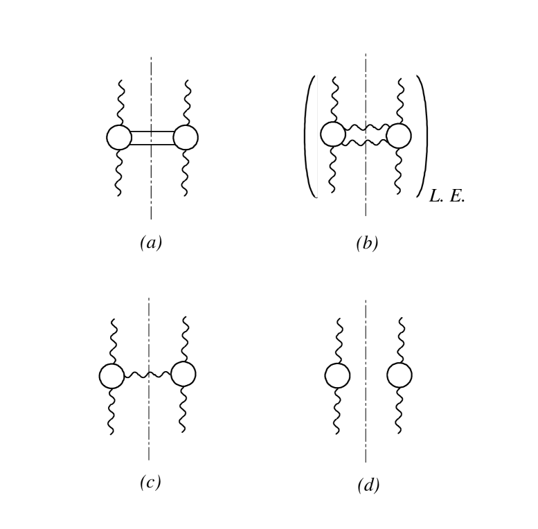
Figure 3: (a) $q\bar{q}$ and (b) low energy $gg$ contributions to the NL kernel, together with (c) one-loop corrections to $1g$ state and (d) two-loop virtual corrections.

The program of computing the NL kernel [11] involves the lowest order computation of the 2-particle $s$-channel discontinuity of the four gluon exchange amplitude, of the one loop correction to the corresponding 1-gluon intermediate state, and of the purely virtual two loop corrections (Fig. 3). Each of these terms can be further divided in sub-terms having different colour structure, according to their dependence on $C_{A}$, $C_{F}$, $N_{f}$. In the following we will concentrate on the $N_{f}$-dependent part, which will be called the $q\bar{q}$ contribution.

Up to now all virtual corrections (to one or no-particle discontinuities) have been computed by Fadin and collaborators [13, 14], while the evaluation of the real emission terms has not been completed. In fact, amplitudes [8, 11] and squared matrix elements for $q\bar{q}$ [8] and gluonic [12] contributions are known in the literature, but the phase-space integrations have not yet been performed.

In the following sections we give the details of our recent computation [16] of the $q\bar{q}$ emission kernel, of its eigenvalues, and of the corresponding anomalous dimension.

3.1 Massive $q\bar{q}$ production

In order to regularize $s$-channel collinear singularities, we will work with massive quarks (the relevant formulas in the massless limit and $4+2\varepsilon$ dimensions will be given in the next section). As an intermediate step, we shall obtain the high energy coefficient function for the $Q\bar{Q}$ production via gluon-gluon fusion.

We thus start by considering the total cross section for the hadroproduction of a (heavy) quark-antiquark pair, which at high energies is dominated by the (Regge) gluon fusion process of Fig. 4. In the large center of mass energy limit the perturbative expansion of this cross section contains large terms of order $\left[\alpha_{s}(M^{2})\log(s/M^{2})\right]^{n}$, which need to be resummed to all orders. This resummation is performed by using the ${\bf k}$-factorized expression for the cross section [8]

$$M^{2}\sigma_{12}=\int\frac{dz_{1}}{z_{1}}\frac{dz_{2}}{z_{2}}d^{2}{\bf k}d^{2}{\bf k}^{\prime}\hat{\sigma}({\bf k},{\bf k}^{\prime},M^{2},z_{1}z_{2}s){\cal F}_{1}(z_{1},{\bf k}){\cal F}_{2}(z_{2},{\bf k}^{\prime}),$$ (3.1)

in which the gluon densities ${\cal F}_{i}$ satisfy the BFKL equation (2.1), and $\hat{\sigma}$ is the (lowest-order and gauge-invariant) off-shell continuation of the partonic cross section.

In the language of $Q^{2}$ and $s$-moments defined in Sec. 2, we introduce the double Mellin transformed version of Eq. (3.1), i.e.,

$$M^{2}\sigma\left(\frac{M^{2}}{s}\right)=\int_{\frac{1}{2}-i\infty}^{\frac{1}{2}+i\infty}\frac{d\gamma_{1}d\gamma_{2}d\omega}{-i(2\pi)^{3}\gamma_{1}\gamma_{2}}\left(\frac{M^{2}}{Q_{0}^{2}}\right)^{\gamma_{1}+\gamma_{2}}{\cal F}_{1\omega}(\gamma_{1}){\cal F}_{2\omega}(\gamma_{2})H_{\omega}(\gamma_{1},\gamma_{2})$$ (3.2)

where

$${\cal F}_{i\omega}(\gamma)=\int^{1}_{0}dzz^{\omega-1}\int_{0}^{\infty}\frac{d^{2}{\bf k}}{\pi{\bf k}^{2}}\left(\frac{{\bf k}^{2}}{Q_{0}^{2}}\right)^{\gamma}{\cal F}_{i}(z,{\bf k})$$ (3.3)

$$H_{\omega}(\gamma_{1},\gamma_{2})=\int_{0}^{\infty}\frac{d^{2}{\bf k}}{{\bf k}^{2}}\frac{d^{2}{\bf k}^{\prime}}{{\bf k}^{\prime 2}}\left(\frac{{\bf k}^{2}}{M^{2}}\right)^{\gamma_{1}}\left(\frac{{\bf k}^{\prime 2}}{M^{2}}\right)^{\gamma_{2}}\int_{0}^{\infty}\frac{ds}{s}\left(\frac{M^{2}}{s}\right)^{\omega}\hat{\sigma}({\bf k},{\bf k}^{\prime},M^{2},z_{1}z_{2}s)$$ (3.4)

For large enough $M^{2}$ the $\gamma$-integrals are dominated by the BFKL anomalous dimensions (2.31), so that the process-dependent high-energy resummation effects are embodied in the coefficient function $H_{\omega}(\gamma_{1},\gamma_{2})$, through the $\omega$-dependence of $\gamma_{1}$ and $\gamma_{2}$. Part of this section is devoted to the evaluation of this coefficient function.

Let us start by defining the kinematics of the process under consideration (Fig. 4). First of all we introduce a Sudakov parametrization of the exchanged gluons’ momenta

$$k^{\mu}\simeq z_{1}p_{1}^{\mu}+{\bf k}^{\mu},\quad\quad k^{\prime\mu}\simeq-z_{2}p_{2}^{\mu}-{\bf k}^{\prime\mu},$$ (3.5)

and of the momentum transfer

$$\Delta^{\mu}=z_{1}x_{1}p_{1}^{\mu}-z_{2}x_{2}p_{2}^{\mu}+\mbox{\boldmath$\Delta$}^{\mu},$$ (3.6)

where $p_{1}$, $p_{2}$ denote the (light-like) momenta of the incoming hadrons. Expressing the phase-space in terms of these variables, the moments in Eq. (3.4) take the form

$$\!\!\!\!\!\!\!\!\!\frac{\alpha_{s}}{\pi}H_{\omega}(\gamma_{1},\gamma_{2})=$$

$$\!\!\!\!\!\!\!\!\!\int\frac{d\nu}{\nu^{2-\omega}}\frac{d^{2}{\bf k}}{\pi{\bf k}^{2}}\frac{d^{2}{\bf k}^{\prime}}{\pi{\bf k}^{\prime 2}}dx_{1}dx_{2}d^{2}\mbox{\boldmath$\Delta$}\delta(x_{2}(1-x_{1})\nu-({\bf k}-\mbox{\boldmath$\Delta$})^{2}-M^{2})\times$$

$$\times\delta(x_{1}(1-x_{2})\nu-(-{\bf k}^{\prime}+\mbox{\boldmath$\Delta$})^{2}-M^{2})\left(\frac{{\bf k}^{2}}{M^{2}}\right)^{\gamma_{1}}\left(\frac{{\bf k}^{\prime 2}}{M^{2}}\right)^{\gamma_{2}}A({\bf k},{\bf k}^{\prime},\mbox{\boldmath$\Delta$},x_{1},x_{2},\nu,M^{2}).$$ (3.7)

Here $A$ denotes the (off-shell) squared matrix element for the (Regge) gluon fusion channel of the $Q\bar{Q}$ production process, and we have defined

$$\nu=z_{1}z_{2}(2p_{1}\cdot p_{2})=z_{1}z_{2}s.$$ (3.8)

In order to understand the colour and singularity structure of the $q\bar{q}$ kernel, in view of the following phase-space integrations, we find it convenient to rewrite the squared matrix element of Ref. [8] in the following form:

$$\frac{A}{\nu^{2}} =\alpha_{s}^{2}(D_{1}+D_{2}+D_{3})$$ (3.9)

where

$$D_{1} =(2C_{F}-C_{A})\left[\frac{-1}{(M^{2}-\hat{t})(M^{2}-\hat{u})}+\frac{(B+C)^{2}}{{\bf k}^{2}{\bf k}^{\prime 2}}\right],$$ (3.10a)

$$D_{2} =C_{A}\left[\frac{1}{\hat{s}}\left(\frac{1}{M^{2}-\hat{u}}-\frac{1}{M^{2}-\hat{t}}\right)(1-x_{1}-x_{2})-\frac{B^{2}+C^{2}}{2{\bf k}^{2}{\bf k}^{\prime 2}}+\right.$$

$$\left.\quad\quad\quad\quad+\frac{2(B-C)}{{\bf k}^{2}{\bf k}^{\prime 2}\hat{s}}\left({\bf k}^{2}(1-x_{2})+{\bf k}^{\prime 2}(1-x_{1})+{\bf k}\cdot{\bf k}^{\prime}\right)\right],$$ (3.10b)

$$D_{3} =C_{A}\left[\frac{2}{\nu\hat{s}}-\frac{2}{{\bf k}^{2}{\bf k}^{\prime 2}}\frac{\left({\bf k}^{2}(1-x_{2})+{\bf k}^{\prime 2}(1-x_{1})+{\bf k}\cdot{\bf k}^{\prime}\right)^{2}}{\hat{s}^{2}}\right],$$ (3.10c)

and we have introduced the notation

$$B= \frac{1}{2}-\frac{(1-x_{1})(1-x_{2})\nu}{M^{2}-\hat{t}}+\frac{\nu(1-x_{1}-x_{2})}{2\hat{s}}+\frac{\mbox{\boldmath$\Delta$}\cdot({\bf k}+{\bf k}^{\prime})}{\hat{s}},$$ (3.11a)

$$C= \frac{1}{2}-\frac{x_{1}x_{2}\nu}{M^{2}-\hat{u}}-\frac{\nu(1-x_{1}-x_{2})}{2\hat{s}}-\frac{\mbox{\boldmath$\Delta$}\cdot({\bf k}+{\bf k}^{\prime})}{\hat{s}},$$ (3.11b)

and the Mandelstam variables of the hard sub-process

$$\hat{s}=(k_{1}+k_{2})^{2},\quad\hat{t}=\Delta^{2}\quad\hat{u}=(k_{1}-k_{2}-\Delta)^{2}.$$ (3.12)

We have decomposed the matrix element (3.9) in the three terms (3.10) in such a way that the integrals over $\nu$ in Eq. (3.7) are separately convergent. Furthermore, all the $s$-channel collinear singularities are contained in the term $D_{3}$ in Eq. (3.10c), since the various poles of the type $1/\hat{s}$ and $1/\hat{s}^{2}$ in (3.10b) cancel each other. This implies that we will be allowed to compute the contribution of $D_{1}$ and $D_{2}$ to the kernel directly in the massless limit and four space dimensions, and only the term $D_{3}$, with its simple structure, will need a regularization.

As a final remark, note that the first term ($\sim(2C_{F}-C_{A})$) is suppressed by a colour factor of $1/C_{A}^{2}$ with respect to the others. We shall see in the following that this suppression factor is relevant in order to assess the magnitude of NL $q\bar{q}$ contributions to the kernel eigenvalue.

The algebra involved in the evaluation of the phase-space integrals in Eq. (3.7) is cumbersome. So we give here only the final result in the $\omega=0$ limit, and we report the details of the phase-space integrations in Appendix A. Following the decomposition (3.9) of the matrix element, we split the moment in Eq. (3.4) in three parts $H^{(1)}$, $H^{(2)}$ and $H^{(3)}$, as follows

$$\!\!\!\!\!\!\!\!\!H_{0}(\gamma_{1},\gamma_{2})=H^{(1)}(\gamma_{1},\gamma_{2})+H^{(2)}(\gamma_{1},\gamma_{2})+H^{(3)}(\gamma_{1},\gamma_{2})$$ (3.13)

where

$$\!\!\!\!\!\!\!\!\!H^{(1)}=(2C_{F}-C_{A})H^{ab}(\gamma_{1},\gamma_{2})$$ (3.14a)

$$\!\!\!\!\!\!\!\!\!H^{(2)}=\frac{\alpha_{s}}{\pi}C_{A}B(\gamma_{1},1-\gamma_{1})B(\gamma_{2},1-\gamma_{2})\left(\frac{\Gamma(2-\gamma_{1}-\gamma_{2})}{\Gamma(4-2\gamma_{1}-2\gamma_{2})}-\frac{\Gamma(3-\gamma_{1}-\gamma_{2})}{\Gamma(6-2\gamma_{1}-2\gamma_{2})}\right)$$ (3.14b)

$$\!\!\!\!\!\!\!\!\!H^{(3)}=\frac{\alpha_{s}}{\pi}C_{A}\frac{B(\gamma_{1},1-\gamma_{1}-\gamma_{2})B(\gamma_{2},1-\gamma_{1}-\gamma_{2})B(2-\gamma_{1}-\gamma_{2},2-\gamma_{1}-\gamma_{2})}{2(1-\gamma_{1}-\gamma_{2})}\times$$

$$\!\!\!\!\!\!\!\!\!\times\left(1-\frac{1}{5-2\gamma_{1}-2\gamma_{2}}\right)$$

and $H^{ab}(\gamma_{1},\gamma_{2})$ is the abelian contribution (2.26).

The result (3.13)-(3.14) provides, in $\gamma$-space, the leading order coefficient for the production of a (heavy) quark-antiquark pair via gluon-gluon fusion, relevant for $Q\bar{Q}$ production in hadron-hadron scattering, and completes the results of Ref. [8] where the $C_{F}$ dependent part was computed.

The above coefficient (in the massless limit) is related to the NL eigenvalue, representing the action of the kernel on the leading order powerlike eigenfunctions $\sim({\bf k}^{2})^{\gamma-1}$. The massless limit, obtained as the residue of the pole at $\gamma_{1}+\gamma_{2}=1$ (Cfr. Eqs. (2.25) and (2.26)), is singular. In fact, due to the $s$-channel collinear singularity of $D_{3}$, the term $H^{(3)}$ in Eq. (3.14c) has triple and double poles, which must be cancelled by the virtual terms.

3.2 Massless quark limit

The triple pole singularity of $H^{(3)}$ in Eq. (3.14c) is due to the singular behaviour of the $gg\rightarrow q\bar{q}$ cross section of Eq. (3.4) in the region $M^{2}\ll({\bf k}-{\bf k}^{\prime})^{2}\equiv{\bf q}^{2}\ll{\bf k}^{2}\simeq{\bf k}^{\prime 2}$. In fact, after phase space integration, the partonic cross section approaches the singular limit

$$\!\!\!\!\!\!\!\!\!\hat{\sigma}_{\omega=0}({\bf k},{\bf k}^{\prime},M^{2})=$$

$$\!\!\!\!\!\!\!\!\!\bar{\alpha_{s}}\frac{\alpha_{s}}{\pi}\int_{0}^{1}dx_{1}\frac{x_{1}(1-x_{1})}{{\bf q}^{2}}\log\left(1+\frac{x_{1}(1-x_{1}){\bf q}^{2}}{M^{2}}\right)\simeq\bar{\alpha_{s}}\frac{\alpha_{s}}{6\pi}\left[\log\frac{{\bf q}^{2}}{M^{2}}-\frac{5}{3}\right]\frac{1}{{\bf q}^{2}}$$ (3.15)

which is responsible for the triple pole, of the ${\bf k}^{2}$-moments in Eq. (3.13).

As remarked before, this singularity comes from the last term $D_{3}$ in Eq. (3.10), while the $s$-channel singularities of $D_{2}$ cancel each other after phase-space integration.

It is interesting to notice that such singular behaviour is responsible for a sizeable enhancement of the $Q\bar{Q}$ hadroproduction cross section at high energies when the two anomalous dimension $\gamma_{1}$ and $\gamma_{2}$ approach the saturating value of $1/2$. On this basis we expect relevant effects due to the resummation of higher orders in the b-quark cross-section at Tevatron, which will be the subject of further investigations.

From the point of view of the $q\bar{q}$ kernel instead, we have still to include the virtual contributions, which are singular also. Having identified the singular real emission part with the $H^{(3)}$ term in Eq. (3.14c), we subtract it off and we perform the massless limit on the finite part, leaving to the next section the combination of $H^{(3)}$ with the virtual radiative corrections, to yield an overall finite result.

In analogy with Eq. (2.25) we then define the regular $q\bar{q}$ contribution to the kernel eigenvalue, as follows

$$\chi_{reg}^{q\bar{q}} =\underset{\gamma_{1}\rightarrow 1-\gamma}{\lim}(1-\gamma-\gamma_{1})\left[H^{(1)}(\gamma,\gamma_{1})+H^{(2)}(\gamma,\gamma_{1})\right]=$$

$$=\frac{C_{A}\alpha_{s}}{6\pi}\left(\frac{\pi}{\sin\pi\gamma}\right)^{2}\left(1-\frac{3(2C_{F}-C_{A})}{C_{A}}\cos(\pi\gamma)\frac{1+\frac{3}{2}\gamma(1-\gamma)}{(3-2\gamma)(1-2\gamma)(1+2\gamma)}\right),$$ (3.16)

which is obtained directly from Eqs. (3.14a) and (3.14b).

For completeness we report the kernel (3.16) in ${\bf k}$-space also. By inverting Eq. (2.4), as explained in Appendix B, we are able to express the azimuthal averaged real emission regular $q\bar{q}$ kernel as follows,

$$K_{reg}^{q\bar{q}} =\frac{1}{{\bf k}^{2}}\int_{\frac{1}{2}-i\infty}^{\frac{1}{2}+i\infty}\frac{d\gamma}{2\pi i}\chi_{reg}^{q\bar{q}}(\gamma)\left(\frac{{\bf k}^{2}}{{\bf k}^{\prime 2}}\right)^{-\gamma}=$$

$$=\frac{2C_{F}-C_{A}}{C_{A}}\frac{N_{f}\alpha_{s}}{64\pi{\bf k}_{>}^{2}}\left[\log\frac{1}{\rho}\left(\frac{1}{\rho}-1\right)+2\left(\frac{1}{\rho}+1\right)+\right.$$

$$\left.+2\left({\cal L}_{2}(\rho)+\log\frac{1}{\rho}{\cal L}_{1}(\rho)\right)\left(22-\rho-\frac{1}{\rho}\right)\right]+$$

$$+\frac{C_{A}\alpha_{s}}{6\pi}\frac{1}{{\bf k}^{2}-{\bf k}^{\prime 2}}\log\frac{{\bf k}^{2}}{{\bf k}^{\prime 2}}.$$ (3.17)

where

$${\cal L}_{1}(\rho)= \frac{1}{\sqrt{\rho}}\arctan(\sqrt{\rho}),$$ (3.18)

$${\cal L}_{2}(\rho)= \frac{1}{2i\sqrt{\rho}}\left(Li_{2}(i\sqrt{\rho})-Li_{2}(-i\sqrt{\rho})\right),$$ (3.19)

$$\rho= \frac{k_{<}^{2}}{k_{>}^{2}},\quad\quad k_{<}=\min(|{\bf k}|,|{\bf k}^{\prime}|),\quad k_{>}=\max(|{\bf k}|,|{\bf k}^{\prime}|),$$ (3.20)

and $Li_{2}$ denotes the Euler Dilogarithm.

4 Complete $q\bar{q}$ Kernel and Anomalous Dimension

4.1 Combining with virtual terms

Let us now consider the contribution to the $q\bar{q}$ kernel of the singular part in Eq. (3.10c), whose $\gamma$-moments yield the term $H^{(3)}$ in Eq. (3.14c) with the triple pole. The singular behaviour for $M^{2}$ and ${\bf q}^{2}\rightarrow 0$ of the cross section (3.15) is cancelled in the total NL kernel by the corresponding singularities in the virtual terms.

In order to cancel the $M^{2}=0$ singularity we need the quark loop contribution to the one-gluon $s$-channel discontinuity, which is simply obtained from the NL reggeon-reggeon-gluon vertex computed in Ref. [13]. By squaring the corresponding amplitude, summing over the polarizations of the emitted gluon and averaging over the azimuth, we get

$$\frac{\alpha_{s}N_{f}}{6\pi}\left(\frac{1}{{\bf q}^{2}}\log\frac{M^{2}}{\mu^{2}}-\frac{1}{{\bf k}^{2}-{\bf k}^{\prime 2}}\log\frac{{\bf k}^{2}}{{\bf k}^{\prime 2}}\right),$$ (4.1)

in which $\mu^{2}$ is the renormalization scale. By combining with the singular $q\bar{q}$ emission part (3.14) we get the $M^{2}$-independent expression

$$\frac{\alpha_{s}N_{f}}{6\pi}\left[\left(\log\frac{{\bf q}^{2}}{\mu^{2}}-\frac{5}{3}\right)\frac{1}{{\bf q}^{2}}-\frac{1}{{\bf k}^{2}-{\bf k}^{\prime 2}}\log\frac{{\bf k}^{2}}{{\bf k}^{\prime 2}}\right].$$ (4.2)

which is still singular for ${\bf q}^{2}=0$.

The same computation can be performed in the massless quark limit and $4+2\varepsilon$ dimensions, to yield the $\varepsilon$-dependent kernel (see Appendix C)

$$\frac{\alpha_{s}N_{f}}{6\pi}\left[\frac{1}{\varepsilon}\frac{\Gamma^{2}(1+\varepsilon)}{\Gamma(1+2\varepsilon)}\left(\frac{{\bf q}^{2}}{\mu^{2}}\right)^{\varepsilon}\frac{1-\frac{5}{3}\varepsilon+\frac{28}{9}\varepsilon^{2}+0(\varepsilon^{3})}{{\bf q}^{2}}-\frac{1}{\varepsilon{\bf q}^{2}}-\frac{1}{{\bf k}^{2}-{\bf k}^{\prime 2}}\log\frac{{\bf k}^{2}}{{\bf k}^{\prime 2}}\right].$$ (4.3)

In order to cancel the ${\bf q}^{2}=0$ singularity we need to combine the above results with the purely virtual terms, which were computed in dimensional regularization in Ref. [14]. This can be done by means of Eq. (4.3), and after the cancellation of the singularities at $\varepsilon=0$, the NL $q\bar{q}$ contribution to the kernel can be expressed directly in 4 dimensions as follows (see Appendix C):

$$K_{0}+K_{1}^{q\bar{q}}= \left(1+\frac{\alpha_{s}N_{f}}{6\pi}\log\frac{{\bf k}^{2}}{\mu^{2}}\right)K_{0}({\bf k},{\bf k}^{\prime})+$$

$$+\frac{\alpha_{s}N_{f}}{6\pi}\left[\left.\left(\log\frac{{\bf q}^{2}}{{\bf k}^{2}}-\frac{5}{3}\right)\frac{1}{{\bf q}^{2}}\right|_{R}-\frac{1}{{\bf k}^{2}-{\bf k}^{\prime 2}}\log\frac{{\bf k}^{2}}{{\bf k}^{\prime 2}}\right]+K_{reg}^{q\bar{q}}({\bf k},{\bf k}^{\prime}),$$ (4.4)

where $K^{q\bar{q}}_{reg}$ is the regular part of the real emission kernel given in Eq. (3.17), and we have factorized the $q\bar{q}$ contribution to the running of $\alpha_{s}$ at the scale ${\bf k}^{2}$ in agreement with the choice of Sec. 2.

We remark that such a choice of the scale of $\alpha_{s}$ is not strictly consequence of our NL calculation, since it fixes only the coefficient of the $\log(1/\mu^{2})$ term, while the upper scale of the logarithm can be changed by changing the scale invariant part of the kernel. However this choice allows the clear discussion of factorization properties of the BFKL equation provided in Sec. 2 (Eqs. (2.35) and (2.36)), and yields the NL coefficient (2.19), induced by the running coupling, which differs from unity only from three loops on.

Finally, we are now able to compute the finite eigenvalue of the scale invariant kernel $K_{1}$ in Eq. (4.4). By using standard identities of type

$$\frac{1}{{\bf k}^{2}-{\bf k}^{\prime 2}}\log\frac{{\bf k}^{2}}{{\bf k}^{\prime 2}}=\int_{0}^{1}\frac{dy}{y{\bf k}^{2}+(1-y){\bf k}^{\prime 2}}$$ (4.5a)

and

$$\int_{0}^{\infty}\frac{d^{2}{\bf k}}{\pi{\bf k}^{2}}\left(\frac{{\bf k}^{2}}{M^{2}}\right)^{\gamma}\frac{1}{(M^{2}+\xi{\bf k}^{2})^{n}}=(M^{2})^{-n}\xi^{-\gamma}B(\gamma,n-\gamma),$$ (4.5b)

we obtain the expression

$$\chi_{1}^{q\bar{q}}= \frac{\alpha_{s}N_{f}}{6\pi}\left[\frac{1}{2}(\chi_{0}^{\prime}(\gamma)+\chi_{0}^{2}(\gamma))-\frac{5}{3}\chi_{0}(\gamma)-\right.$$

$$\left.-\frac{1}{N_{C}^{2}}\left(\frac{\pi}{\sin\pi\gamma}\right)^{2}3\cos(\pi\gamma)\frac{1+\frac{3}{2}\gamma(1-\gamma)}{(3-2\gamma)(1-2\gamma)(1+2\gamma)}\right]$$ (4.6)

which is plotted in Fig. 5 as a function of $\gamma$.

Note that the expression (4.6) is symmetrical for $\gamma\rightarrow 1-\gamma$, apart from the $\chi^{\prime}_{0}(\gamma)$ term, which is due to our choice of ${\bf k}^{2}$ as scale of $\alpha_{s}$, instead of a more symmetrical combination of ${\bf k}$ and ${\bf k}^{\prime}$.

4.2 Eigenvalue properties and anomalous dimension

From the plot of Fig. 5 it is evident that a cancellation between terms with different colour structure is at work. In fact, the last term in the eigenvalue (4.6) is essentially the abelian one of Eq. (2.26), except that it is multiplied by the small colour factor $1/N_{C}^{2}$. This means that the non planar diagrams are the ones responsible for the large resummation effects, giving large contributions at high values of both ${\bf k}^{2}$ and ${\bf k}^{\prime 2}$. In fact, they are suppressed in the large $N_{C}$ limit when coupled to gluons in $K_{1}$, but are not when coupled to photons in $H_{2}$ (Eq. (2.26)).

From Eq. (4.6) the part of the shift of the pomeron intercept which is proportional to $N_{f}$ can be estimated. For models with a continuum spectrum [20] it is simply obtained by setting $\gamma=1/2$, to yield

$$\Delta\omega_{\mathbb{P}}=\omega_{\mathbb{P}}\frac{\alpha_{s}N_{f}}{6\pi}\left[2\log 2-\frac{5}{3}-\frac{1}{N_{C}^{2}}\frac{33}{32}\frac{\pi^{3}}{8\log 2}\right],$$ (4.7)

$$= \frac{\Delta\omega_{\mathbb{P}}}{\omega_{\mathbb{P}}}\simeq-0.05N_{f}\alpha_{s},$$ (4.8)

which is just a few percent for reasonable values of $N_{f}$ and $\alpha_{s}$. Once again, the potentially large term $\sim\pi^{3}$ is suppressed by a colour factor.

In order to compute the NL correction to the anomalous dimensions, we introduce the ’renormalized’ coupling

$$\bar{\alpha_{s}}\rightarrow\tilde{\alpha_{s}}=\bar{\alpha_{s}}\left(1+\frac{\Delta\omega_{\mathbb{P}}}{\omega_{\mathbb{P}}}\right).$$ (4.9)

in the defining equation (2.29), so that it takes the form

$$1=\frac{\tilde{\alpha_{s}}}{\omega}\left[\chi_{0}(\gamma_{+})+\alpha_{s}\left(\chi_{1}(\gamma_{+})-\chi_{1}(1/2)\right)\right]$$ (4.10)

and then we expand $\gamma_{+}$ in the $\chi_{0}$-term around $\gamma_{+}=\gamma^{L}(\tilde{\alpha_{s}})$, to get

$$\left[\gamma_{+}-\gamma_{L}\right]^{q\bar{q}}=\alpha_{s}\frac{\chi_{1}^{q\bar{q}}(\gamma_{L})-\chi_{1}^{{\bf q}\bar{q}}(1/2)}{-\chi_{o}^{\prime}(\gamma_{L})},$$ (4.11)

$$1=\tilde{\alpha_{s}}\chi_{0}(\gamma_{L}).$$ (4.12)

In this way the perturbative expansion in powers of $\gamma_{L}(\tilde{\alpha_{s}})$ is free of spurious singularities for $\gamma_{L}=1/2$, which would signal precisely a renormalization of the Pomeron intercept.

The NL correction (4.11) to the leading eigenvalue of the anomalous dimension matrix $\gamma_{+}$ is plotted in Fig. 6 as a function of $\gamma_{L}(\tilde{\alpha_{s}})$. This correction is small compared to the leading anomalous dimension $\gamma_{L}$, apart from the region of very small $\gamma_{L}$ corresponding to $\omega\geq\alpha_{s}$, where it is needed in order to achieve consistency with fixed order renormalization group equation. Therefore, higher order effects are negligible.

A particular comment is needed on how fixed order perturbation theory is recovered in this formalism. In fact, since $\gamma_{L}=\bar{\alpha_{s}}/\omega+O(\bar{\alpha_{s}}^{4})$, the small $\gamma$ behaviour of $\chi_{1}(\gamma)$ in Eq. (4.11) determines directly the one and two loop anomalous dimensions:

$$\gamma_{+}-\gamma_{L}\simeq\frac{\alpha_{s}N_{f}}{6\pi}\left[-\frac{1}{N_{C}^{2}}-\frac{5}{3}\left(1+\frac{13}{10N_{C}^{2}}\right)\frac{\bar{\alpha_{s}}}{\omega}+....\quad\right]$$ (4.13)

and from Eq. (2.31) we obtain

$$\gamma_{gg}\simeq-\frac{\alpha_{s}N_{f}}{6\pi}\left(1+\frac{23}{6}\frac{\bar{\alpha_{s}}}{\omega}+....\quad\right)$$ (4.14)

which agrees with the two loop computation in the DIS scheme [26].

More in general, we can say that if

$$\gamma_{+}^{(1)}=\frac{\bar{\alpha_{s}}}{\omega}+A_{1}\alpha_{s},\quad\quad\gamma_{+}^{(2)}=A_{2}\alpha_{s}\frac{\bar{\alpha_{s}}}{\omega}$$ (4.15)

is the NL expression at two loop order, the eigenvalue $\chi_{1}$ should have the structure

$$\chi_{1}(\gamma)\simeq\frac{A_{1}}{\gamma^{2}}+\frac{A_{2}}{\gamma}+(\gamma\rightarrow 1-\gamma)+\text{running coupling terms}$$ (4.16)

just on the basis of the $\gamma=0$ singularities needed to recover (4.14) and of the basic ${\bf k}\rightarrow{\bf k}^{\prime}$ symmetry of the BFKL kernel - apart from the asymmetry induced by factorizing out $\alpha_{s}({\bf k}^{2})$ in Eq. (4.4).

The singularities at $\gamma=0$ occurring in Eq. (4.16) are just the collinear ones coming from transverse momenta $|{\bf k}|\gg\Delta\gg|{\bf k}^{\prime}|$, while the ones at $\gamma=1$ come from the disordered region ($|{\bf k}^{\prime}|\gg\Delta\gg|{\bf k}|$), that we have already emphasized [25] as a possible source of large higher order effects. The third possible source of collinear singularities - the one in the $s$-channel - turns out to combine with virtual corrections to give rise to running coupling effects added in Eq. (4.16).

The structure of Eqs. (4.15) and (4.16) is interesting for various reasons. Firstly, it appears that the NL terms arise from various collinear singular kernels, as already emphasized in Eqs. (2.33)-(2.34) at one-loop level. This is because the two channel collinear factorization is not disentangled yet in the BFKL approach (Cfr. Sec. 2.2).

Secondly, we can follow the suggestion of Ref. [25], and use the expression (4.16), including the $(1-\gamma)$-terms, as a crude estimate of $\chi_{1}$ for the gluonic contribution, where a complete calculation is not yet available. In that case we should set

$$A_{1}=-\frac{\alpha_{s}N_{f}}{6\pi}\frac{1}{N_{C}^{2}}-\frac{11N_{C}\alpha_{s}}{12\pi},\quad\quad A_{2}=-\frac{\alpha_{s}N_{f}}{6\pi}\left(\frac{5}{3}+\frac{13}{6N_{C}^{2}}\right)$$ (4.17)

with the rough estimate

$$\chi_{1,coll}=\chi_{1,coll}^{(q\bar{q})}-\frac{11N_{C}\alpha_{s}}{12\pi}\left(\frac{1}{\gamma^{2}}+\frac{1}{(1-\gamma)^{2}}\right)+....$$ (4.18)

The last term in Eq. (4.18) is large, and - if extended to large $\gamma$ values - would provide a negative and sizeable shift of the Pomeron intercept and important resummation effects, unlike what happens for the $q\bar{q}$ contribution.

Although we do not think the estimate (4.18) is reliable when approaching $\gamma=1/2$, it provides an indication of the existence of unsuppressed planar contributions in the gluonic part. The complete calculation is therefore a rather important goal to achieve.

5 Discussion

We have studied in this paper the anomalous dimension representation for the NL BFKL equation and the ensuing resummation formulas, by analysing in detail the $q\bar{q}$ contributions to the larger anomalous dimension eigenvalue.

Our first result (Sec. 2) is that the R.G. representation with running coupling and resummed anomalous dimensions is valid at NL level in the regime

$$t=\log\frac{Q^{2}}{\Lambda^{2}}\gg 1,\bar{b}\omega t>\chi\left(\frac{1}{2}\right),$$ (5.1)

that is, if the variable $\alpha_{s}(t)\log\frac{1}{x}$ is not too large. If the condition (5.1) is coupled with the saddle point estimate of important $\omega$ values we end up with the limitation

$$\bar{\alpha}_{S}(t)\log\frac{1}{x}<\frac{1}{\chi\left(\frac{1}{2}\right)}\left(\log{\frac{t}{t_{0}}}\right)t,$$ (5.2)

which provides a parabola-like boundary in the $\log\frac{1}{x}$, $\log\frac{Q^{2}}{\Lambda^{2}}$ plane.

Conditions of type (5.1) have been already noticed before [22] as singularities of the anomalous dimension and those of the type (5.2) have been known for a while [21] to be relevant, with different numerical factors, for the occurrence of higher twist unitarization effects [27-29]. Here we just emphasize that, within the regions (5.1) and (5.2) there is a well defined resummation of anomalous dimensions, provided here, which is able to describe the QCD evolution in agreement with the NL BFKL equation (Fig 7).

The renormalization group description in the regime (5.1) holds independently of the detailed properties of the hard Pomeron, i.e. of the leading singularity in the $\omega$-plane which dominates the small-$x$, fixed $Q^{2}$ behaviour. The latter occurs in the coefficient function, and is dependent on the soft region behaviour of the running coupling, in particular on its magnitude and shape around ${\bf k}^{2}=\Lambda^{2}$. Only if the scale ${Q_{0}}^{2}$ is large enough, the Pomeron decouples, and the coefficient function takes a perturbative form, provided the rapidity is not so large to allow diffusion from ${Q_{0}}^{2}$ to $\Lambda^{2}$.

The simplest way to summarize the above results is to write the resummed R.G. representation of the DIS structure functions $F_{2}$ and $F_{L}$. By using formulas (2.35) for the parton densities in the $Q_{0}$-scheme we obtain

$$\begin{pmatrix}F_{2}^{A}(Q^{2})\\ F_{L}^{A}(Q^{2})\end{pmatrix}=\begin{pmatrix}\gamma_{+}H_{2}(\gamma_{+})\\ \gamma_{+}H_{L}(\gamma_{+})\end{pmatrix}G_{+}^{A}+\begin{pmatrix}-\frac{C_{A}}{C_{F}}\\ \frac{\alpha_{s}}{3\pi}\end{pmatrix}G_{-}^{A}$$ (5.3)

where $H_{2}$ and $H_{L}$ are given by Eq. (2.26) and by the relation [10]

$$H_{L}(\gamma)=\frac{\gamma(1-\gamma)}{1+\frac{3}{2}\gamma(1-\gamma)}H_{2}(\gamma)$$ (5.4)

respectively, and ${G_{\pm}}^{A}$ are the R.G. expressions of Eq. (2.36). In particular,

$$G_{+}^{A}=\frac{1}{\gamma_{+}\sqrt{-\chi^{\prime}(\gamma_{+})}}\exp\left[\int_{0}^{t}\gamma_{+}(\alpha_{s}(t))dt\right]$$ (5.5)

contains the perturbative coefficient of Eq. (2.19), which provides an additional contribution to the effective anomalous dimension of Eq. (2.38).

Note that, once a complete NL computation of $\gamma_{+}$ will be available, all the relevant coefficient and anomalous dimensions in Eq. (5.3) will be known in the $Q_{0}$-scheme, so as to provide a factorization scheme independent expression for the measurable structure functions.

In fact, relating Eqs. (5.3) and (2.35) is equivalent to computing the quark and gluon coefficient functions in the $Q_{0}$-scheme to all leading orders. By simple algebra, and neglecting subleading contributions, we get

$$\!\!\!\!\!\!\!\!\!C_{q}^{2}=1, C_{g}^{2}=0;$$ (5.6)

$$\!\!\!\!\!\!\!\!\!C_{q}^{L}=\frac{C_{F}N_{f}}{C_{A}}\left[\gamma_{+}H_{L}(\gamma_{+})-\frac{\alpha_{s}}{3\pi}\right], C_{g}^{L}=\gamma_{+}H_{L}(\gamma_{+}).$$ (5.7)

In this paper we have further provided a computation of the $q\bar{q}$-contribution to the BFKL kernel, proving the running coupling factorization, and we have evaluated the corresponding NL resummation in the anomalous dimension eigenvalue $\gamma_{+}$.

We find that higher order effects for the $N_{f}$ dependent part are small in $\gamma_{+}$, while they are not small in the coefficients $H_{2}$ and $H_{L}$. This difference is due to the non-planar nature of the diagrams which yield the most important large ${\bf k}$ contributions. They are suppressed by a colour factor when coupling to gluons, while they are not when coupling to photons.

We have also found that running coupling effects, although expected, are particularly important. First of all, they affect the coefficient functions by factors of type $H$ in Eqs. (2.19) and (5.5) due to the fluctuations of the anomalous dimension variable $\gamma$, which are large when $\gamma$ approaches the saturation value $\gamma=1/2$. Ultimately, this is the reason for the breaking of the R. G. representation itself when approaching the critical value (5.1), as also noticed in a recent paper [30].

Furthermore, the running of $\alpha_{s}(t)\simeq 1/bt$ at large $t$ values, emphasizes the diffusion towards small values of ${\bf k}^{2}$, and the need of smoothing out the effective coupling around the Landau pole. This in turn clarifies the fact that the bare hard Pomeron singularity is actually dependent on soft physics, even if small-$x$ scaling violations are not.

It thus appears that, so far, apart from running coupling effects, large higher order contributions only occur in the $\gamma_{qg}$ entry of the anomalous dimension matrix, which was the basis for an early explanation of the HERA data [4]. Note, however, that the absence of higher order effects in $\gamma_{+}$ may be a feature of the $N_{f}$-dependent part only, which is mostly nonplanar. For the gluonic part, planar diagrams could also contribute, as it happens in the crude collinear estimate of Eq. (4.18). Such possibly large effects renew the present interest in a complete computation, which is hopefully to be obtained soon.

Acknowledgements

We wish to thank Jochen Bartels, Stefano Catani, Yuri Dokshitzer, Jan Kwiecinski, Al Mueller and Bryan Webber for interesting discussions on the topics presented here. This work is supported in part by MURST, Italy, and by the E. C. contract CHRX-CT96-0357.

Appendix A: Kinematics and Integrals

We give here some details of the computation of the $H_{0}$ function (3.13).

Starting from the Sudakov parametrization (3.5)-(3.6) of the relevant momenta, we write the two-body phase space of the produced $q\bar{q}$ pair as follows

$$\!\!\!\!\!\!\!\!\!\!\!\!\!\!\!\!\!\!d\Phi(1,2) =\frac{\nu}{8\pi^{2}}dx_{1}dx_{2}d^{2}\mbox{\boldmath$\Delta$}\delta(x_{2}(1-x_{1})\nu-({\bf k}-\mbox{\boldmath$\Delta$})^{2}-M^{2})\times$$

$$\times\delta(x_{1}(1-x_{2})\nu-(-{\bf k}^{\prime}+\mbox{\boldmath$\Delta$})^{2}-M^{2})=$$ (A.1a)

$$=\frac{1}{8\pi}\frac{dx_{1}}{x_{1}(1-x_{1})}\frac{d^{2}\tilde{\mbox{\boldmath$\Delta$}}}{2\pi}\delta\left(\nu-\frac{\tilde{\mbox{\boldmath$\Delta$}}^{2}+M^{2}}{x_{1}(1-x_{1})}-{\bf q}^{2}\right)=$$ (A.1b)

$$=\frac{1}{8\pi}\frac{dx_{2}}{x_{2}(1-x_{2})}\frac{d^{2}\hat{\mbox{\boldmath$\Delta$}}}{2\pi}\delta\left(\nu-\frac{\hat{\mbox{\boldmath$\Delta$}}^{2}+M^{2}}{x_{2}(1-x_{2})}-{\bf q}^{2}\right),$$ (A.1c)

where

$$\tilde{\mbox{\boldmath$\Delta$}}=\mbox{\boldmath$\Delta$}-{\bf k}x_{1}-{\bf k}^{\prime}(1-x_{1}),$$ (A.2a)

$$\hat{\mbox{\boldmath$\Delta$}}=\mbox{\boldmath$\Delta$}-{\bf k}^{\prime}x_{2}-{\bf k}(1-x_{2})..$$ (A.2b)

So, since the hard cross section is related to the matrix element by

$$\hat{\sigma}({\bf k},{\bf k}^{\prime},M^{2},\nu)=\frac{1}{2\nu}\int d\Phi(1,2)A({\bf k},{\bf k}^{\prime},\mbox{\boldmath$\Delta$},x_{1},x_{2},M^{2}),$$ (A.3)

we get, by (A.1a), the expression (3.7).

Since both parametrizations of the phase-space (A.1b) and (A.1c) are needed in the computation of the integrals, for each of them we give the expression of the relevant scalar quantities. Starting with the former, we have

$$\hat{s}= \frac{\tilde{\mbox{\boldmath$\Delta$}}^{2}}{x_{1}(1-x_{1})},$$ (A.4)

$$M^{2}-\hat{t}= (1-x_{1})(\hat{s}+{\bf k}^{2})+x_{1}{\bf k}^{\prime 2}-2\tilde{\mbox{\boldmath$\Delta$}}\cdot{\bf k}^{\prime},$$ (A.5)

$$M^{2}-\hat{u}= x_{1}(\hat{s}+{\bf k})^{2}+(1-x_{1}){\bf k}^{\prime 2}-2\tilde{\mbox{\boldmath$\Delta$}}\cdot{\bf k}^{\prime},$$ (A.6)

$$x_{2}= \frac{\left[(1-x_{1}){\bf q}-\tilde{\mbox{\boldmath$\Delta$}}\right]^{2}+M^{2}}{(1-x_{1})\nu},$$ (A.7)

for the latter

$$\hat{s}= \frac{\hat{\mbox{\boldmath$\Delta$}}^{2}+M^{2}}{x_{2}(1-x_{2})},$$ (A.8)

$$M^{2}-\hat{t}= (1-x_{2})(\hat{s}+{\bf k}^{\prime 2})+x_{2}{\bf k}^{2}-2\hat{\mbox{\boldmath$\Delta$}}\cdot{\bf k},$$ (A.9)

$$M^{2}-\hat{u}= x_{2}(\hat{s}+{\bf k}^{\prime 2})+(1-x_{2}){\bf k}^{2}+2\hat{\mbox{\boldmath$\Delta$}}\cdot{\bf k},$$ (A.10)

$$x_{1}= \frac{\left[(1-x_{2}){\bf q}+\hat{\mbox{\boldmath$\Delta$}}\right]^{2}+M^{2}}{(1-x_{2})\nu},$$ (A.11)

and for both of them

$$\nu= \hat{s}+{\bf q}^{2},$$ (A.12)

$${\bf q}= {\bf k}-{\bf k}^{\prime}.$$ (A.13)

In order to compute $H_{0}$, we find it convenient to choose, for each term in the matrix element (3.9), the most suitable phase space parametrization of type (A.1b) or (A.1c). The choice is done by requiring that the denominator of each term in the matrix element (3.9) contains at most two of the invariants given before, and that at most one non-trivial azimuthal integration is needed. It is straightforward to check that at least one of our parametrizations satisfies these requirements for every term in Eqs. (3.9) and (3.10).

With these premises we first use the $\delta$-function in (A.1b) or (A.1c) to eliminate the variable $\nu$, then, with the help of a Feynman parametrization of the denominators, we perform the integration over the transverse components of the momentum transfer $\Delta$. In order to compute the $H_{0}$ function, the best way is to evaluate the ${\bf k}^{2}$-moments at this stage, since all the integrals needed can be reduced to the forms

$$\int_{0}^{\infty}\frac{d^{2}{\bf k}}{\pi{\bf k}^{2}}\left(\frac{{\bf k}^{2}}{M^{2}}\right)^{\gamma}\frac{1}{(M^{2}+\xi{\bf k}^{2})^{n}}=(M^{2})^{-n}\xi^{-\gamma}B(\gamma,n-\gamma)$$ (A.14)

$$\int_{0}^{\infty}\frac{d^{2}{\bf k}_{1}}{\pi{\bf k}_{1}^{2}}\frac{d^{2}{\bf k}_{2}}{\pi{\bf k}_{2}^{2}}\left(\frac{{\bf k}_{1}^{2}}{M^{2}}\right)^{\gamma_{1}}\left(\frac{{\bf k}_{2}^{2}}{M^{2}}\right)^{\gamma_{2}}\frac{1}{(M^{2}+\xi_{1}{\bf k}_{1}^{2}+\xi_{2}{\bf k}_{2}^{2})^{n}}=$$

$$=(M^{2})^{-n}\xi_{1}^{-\gamma_{1}}\xi_{2}^{-\gamma_{2}}\frac{\Gamma(\gamma_{1})\Gamma(\gamma_{2})\Gamma(n-\gamma_{1}-\gamma_{2})}{\Gamma(n)}$$ (A.15)

$$\int_{0}^{\infty}\frac{d^{2}{\bf k}_{1}}{\pi{\bf k}_{1}^{2}}\frac{d^{2}{\bf k}_{2}}{\pi{\bf k}_{2}^{2}}\left(\frac{{\bf k}_{1}^{2}}{M^{2}}\right)^{\gamma_{1}}\left(\frac{{\bf k}_{2}^{2}}{M^{2}}\right)^{\gamma_{2}}\frac{1}{[M^{2}+\xi({\bf k}_{1}+{\bf k}_{2})^{2}]^{n}}=$$

$$=(M^{2})^{-n}\xi^{-\gamma_{1}-\gamma_{2}}\frac{\Gamma(n+1-\gamma_{1}-\gamma_{2})\Gamma(1-\gamma_{1}-\gamma_{2})\Gamma(\gamma_{1})\Gamma(\gamma_{2})}{\Gamma(n)\Gamma(1-\gamma_{1})\Gamma(1-\gamma_{2})}.$$ (A.16)

The remaining integrals over the longitudinal momentum fractions and the Feynman parameters are evaluated in a straightforward way in terms of Gamma and Beta functions, the only trouble being the number of terms, about one hundred. After doing the Gamma -function algebra the result (3.13) is found.

Appendix B: The kernel in ${\bf k}$-space

The inverse Mellin transform needed to compute the regular kernel (3.15) in transverse momentum space involves integrals of the type

$$\int_{\frac{1}{2}-i\infty}^{\frac{1}{2}+i\infty}\frac{d\gamma}{2\pi i}x^{-\gamma}\left(\frac{\pi}{\sin\pi\gamma}\right)^{2}R(\gamma),$$ (B.1)

where $x={\bf k}^{2}/{\bf k}^{\prime 2}$ and $R(\gamma)$ is a holomorphic function of $\gamma$, symmetric under the transformation $\gamma\rightarrow 1-\gamma$, which is provided by the eigenvalue (3.16).

Integrals of this type can be evaluated by closing the contour on the l. h. poles for $x<1$ and on the r. h. ones for $x>1$, so that they reduce to infinite series. Due to the simple structure of $R(\gamma)$, all the integrals can be expressed in terms of the following basic series

$$\sum_{n=0}^{\infty}x^{n}=\frac{1}{1-x},$$ (B.2)

$$\sum_{n=0}^{\infty}\frac{(-1)^{n}x^{n}}{n+\frac{1}{2}}=\frac{2}{\sqrt{x}}\arctan(\sqrt{x}),$$ (B.3)

$$\sum_{n=0}^{\infty}\frac{(-1)^{n}x^{n}}{(n+\frac{1}{2})^{2}}=\frac{2}{i\sqrt{x}}\left(Li_{2}(i\sqrt{x})-Li_{2}(-i\sqrt{x})\right),$$ (B.4)

where $Li_{2}$ denotes the Euler Dilogarithm.

By introducing the expression of the regular eigenvalue (3.16) in (B.1) and performing the $\gamma$-integrals as described above, the expression (3.17) for the kernel in ${\bf k}$ space follows.

Appendix C: Dimensional Regularization

The peculiarity of working in $4+2\varepsilon$ dimensions is that the kernel is dependent on $\varepsilon$ as a regularization parameter, while its eigenvalues are finite (for $\varepsilon\rightarrow 0$). Therefore, in order to compute the $q\bar{q}$ contribution to the kernel eigenvalue in dimensional regularization we have to compute the action of the ($\varepsilon$-dependent) real and virtual contributions on a set of test functions. By adding the various terms, the cancellation of collinear $s$-channel singularities comes out, and the finite $q\bar{q}$ contribution to the NL eigenvalue is obtained. Since we want to show that the NL kernel has the form (2.1), we find it convenient to apply the kernel to the powerlike eigenfunctions of the leading kernel, i. e.

$$f_{\gamma}({\bf k}^{2})=({\bf k}^{2})^{\gamma-1}.$$ (C.1)

C.1 Real $q\bar{q}$ emission

Let us first notice that the collinear singularities are all contained in the term $D_{3}$ in Eq. (3.10c), so that $D_{1}$ and $D_{2}$ can be computed directly in 4 space dimensions by taking the residue at the simple pole for $\gamma_{1}+\gamma_{2}=1$, along the lines of Eq. (2.25). The $D_{3}$ term can be evaluated as follows.

After a simple algebra we find

$$D_{3}=\frac{2}{\nu\hat{s}}\left[1-2(1-x_{1})^{2}+2x_{1}(1-x_{1})\right]+$$ (C.2)

$$+\frac{1}{\hat{s}}\quad\text{or}\quad\frac{1}{\hat{s}^{2}}\quad\text{terms,}$$ (C.3)

where in the last line we refer to terms of the form

$$\frac{P(x_{1})({\bf k}^{2})^{\alpha}({\bf k}^{\prime 2})^{\beta}}{\hat{s}^{n}}$$ (C.4)

(where $P(x_{1})$ is a polynomial in $x_{1}$), which just vanish in dimensional regularization.

By multiplying Eq. (C.2) by the eigenfunction of the real kernel in Eq. (C.1) and introducing the $4+2\varepsilon$ dimensional phase-space integrals over the internal momentum transfer $\Delta$ and the transverse momentum of the emitted $q\bar{q}$ pair, we get

$$D_{3}\otimes f_{\gamma}({\bf k})=$$

$$=(4\pi\mu^{2})^{-2\varepsilon}\alpha_{s}N_{f}\int d^{2(1+\varepsilon)}{\bf q}d^{2(1+\varepsilon)}\mbox{\boldmath$\Delta$}\int_{0}^{1}dx_{1}(1-x_{1})dy[({\bf k}+{\bf q})^{2}]^{\gamma-1}\times$$

$$\times\frac{1+2x_{1}(1-x_{1})-2(1-x_{1})^{2}}{[\mbox{\boldmath$\Delta$}^{2}+x_{1}(1-x_{1})y{\bf q}^{2}]^{2}},$$ (C.5)

where a Feynman parametrization of the denominator $\sim 1/(\nu\hat{s})$ has also been introduced. The integrals in (C.4) can be evaluated by first integrating over the two transverse momenta $\Delta$ and ${\bf q}$, and then on the longitudinal momentum transfer $x_{1}$ and the Feynman parameter $y$. The final result is easily expressed in terms of $\Gamma$-functions, as follows

$$\!\!\!\!\!\!\!\!\!D_{3}\otimes f_{\gamma}({\bf k})=$$

$$\!\!\!\!\!\!\!\!\!=\!\left(\frac{{\bf k}^{2}}{4\pi\mu^{2}}\right)^{2\varepsilon}\!\!\frac{N_{f}\alpha_{s}}{16\pi}\frac{1}{\varepsilon^{2}}\frac{\Gamma(1\!-\!\gamma\!-\!2\varepsilon)\Gamma(\gamma\!+\!\varepsilon)\Gamma(1\!+\!2\varepsilon)\Gamma^{2}(1\!+\!\varepsilon)}{\Gamma(1-\gamma)\Gamma(\gamma+3\varepsilon)}\left[\frac{1}{\Gamma(2+2\varepsilon)}-\frac{2(1+\varepsilon)}{\Gamma(4+2\varepsilon)}\right],$$ (C.6)

and has the following expansion around $\varepsilon=0$

$$({\bf k}^{2})^{\gamma-1}\left(\frac{{\bf k}^{2}}{4\pi\mu^{2}}\right)^{2\varepsilon}\frac{N_{f}\alpha_{s}}{12\pi}\left[\frac{1}{\varepsilon^{2}}+\frac{1}{\varepsilon}\left(2\chi_{0}(\gamma)-\frac{5}{3}\right)+2\psi^{\prime}(1-\gamma)-4\psi^{\prime}(\gamma)+\right.$$

$$\left.+2\chi_{0}^{2}(\gamma)-\frac{10}{3}\chi_{0}(\gamma)+\frac{28}{9}\right].$$ (C.7)

Note that in $4+2\varepsilon$ dimensions, due to the lack of scale-invariance of the kernel, the powers of ${\bf k}^{2}$ are no longer eigenfunctions of the kernel, and are in fact multiplied by powers of $({\bf k}^{2}/\mu^{2})^{\varepsilon}$. Anyway, after the combination with virtual terms, the $\varepsilon\rightarrow 0$ limit will be taken, and it will be possible to isolate the non scale-invariant terms (related to the running of $\alpha_{s}$), from the scale-invariant NL corrections. In performing this procedure we are obliged to expand all partial results up to relative order $\varepsilon^{2}$, because of the double poles occurring in Eq. (C.7).

C.2 Vertex corrections

The vertex corrections to the 1-gluon production amplitude have been computed in Ref. [13] ($N_{f}$-dependent part) and [11] ($N_{f}$-independent part). In the following only the $N_{f}$-dependent part will be considered.

By squaring the 1-gluon production amplitude, together with its one-loop corrections [13] and summing over the emitted gluon’s polarization, the contribution to the kernel in $4+2\varepsilon$ dimensions is readily obtained, as follows

$$\frac{N_{f}\alpha_{s}}{6\pi}\left(\frac{{\bf k}^{2}}{4\pi\mu^{2}}\right)^{\varepsilon}(4\pi)^{-\varepsilon}\Gamma^{2}(1-\varepsilon)\left[\frac{1}{\varepsilon}\frac{1}{{\bf q}^{2}}-\frac{1}{{\bf k}^{2}-{\bf k}^{\prime 2}}\log\frac{{\bf k}^{2}}{{\bf k}^{\prime 2}}\right]+$$

$$\text{terms of order $\varepsilon$ and finite for ${\bf q}=0$}.$$ (C.8)

The action of this part of the (regularized) kernel on the leading order eigenfunctions $f_{\gamma}({\bf k})$ is obtained by performing the integration over ${\bf q}$ in $4+2\varepsilon$ dimensions. However, only the first term in (C.8) needs be regularized, while the second one is finite in both the $\varepsilon=0$ and ${\bf q}=0$ limit.

The second term is easily computed in four dimensions, by using the integral representation

$$\frac{1}{{\bf k}^{2}-{\bf k}^{\prime 2}}\log\frac{{\bf k}^{2}}{{\bf k}^{\prime 2}}=\int_{0}^{1}\frac{dy}{y{\bf k}^{2}+(1-y){\bf k}^{\prime 2}}$$ (C.9)

and then performing the ${\bf k}^{\prime}$ and $y$ integrations according to the standard techniques of Appendix A, to yield the result

$$\frac{N_{f}\alpha_{s}}{6\pi}\left(\frac{\pi}{\sin\pi\gamma}\right)^{2}.$$ (C.10)

The first term in Eq. (C.6) is computed by means of a Feynman parametrization to combine the two powers $1/{\bf q}^{2}$ and $[({\bf k}+{\bf q})^{2}]^{\gamma-1}$, and then performing the $2+2\varepsilon$-dimensional integration over ${\bf q}$ with the standard techniques of dimensional regularization. The final integral over the Feynman parameter is straightforward so that the contribution of the kernel (C.6) can be expressed as

$$\!\!\!\!\!\!\!\!\!-\frac{1}{\varepsilon^{2}}\frac{\Gamma(1-\gamma-\varepsilon)\Gamma(1+\varepsilon)\Gamma(\gamma+\varepsilon)}{\Gamma(1-\gamma)\Gamma(\gamma+2\varepsilon)\Gamma(1-\varepsilon)}\frac{\alpha_{s}N_{f}}{6\pi}\left(\frac{{\bf k}^{2}}{4\pi\mu^{2}}\right)^{\varepsilon}\Gamma^{2}(1-\varepsilon)(4\pi)^{-\varepsilon}+$$

$$-\left(\frac{\alpha_{s}N_{f}}{6\pi}\right)\left(\frac{\pi}{\sin\pi\gamma}\right)^{2}.$$ (C.11)

In the $\varepsilon=0$ limit, (C.11) has the expansion

$$\!\!\!\!\!\!\!\!\!-\frac{\alpha_{s}N_{f}}{6\pi}\left(\frac{{\bf k}^{2}}{4\pi\mu^{2}}\right)^{\varepsilon}\Gamma^{2}(1-\varepsilon)\left[\frac{1}{\varepsilon^{2}}+\frac{\chi_{0}(\gamma)}{\varepsilon}+\frac{1}{2}\left(\chi_{0}^{2}(\gamma)+\psi^{\prime}(\gamma)-3\psi^{\prime}(\gamma)\right)-\left(\frac{\pi}{\sin\pi\gamma}\right)^{2}\right].$$ (C.12)

C.3 Trajectory correction and finiteness of the kernel:

The purely virtual two loop contribution was computed in Ref. [14]. The $N_{f}$-dependent part has the following series expansion around $\varepsilon=0$

$$\delta^{2+2\varepsilon}({\bf q})\left(\frac{{\bf k}^{2}}{4\pi\mu^{2}}\right)^{\varepsilon}\frac{N_{f}\alpha_{s}}{12\pi}\left[\frac{2(4\pi)^{-\varepsilon}}{\varepsilon^{2}}+\left(\frac{{\bf k}^{2}}{4\pi\mu^{2}}\right)^{\varepsilon}\left(-\frac{1}{\varepsilon^{2}}+\frac{5}{3}\frac{1}{\varepsilon}-\frac{28}{9}\right)\right].$$ (C.13)

By integrating the above result over the phase-space $d^{2+2\varepsilon}{\bf q}$ and by combining it with the real emission contribution (C.7) and the vertex correction (C.12), the action of the total NL $q\bar{q}$ kernel on the leading order eigenfunction $f_{\gamma}({\bf k})$ is finally found, as follows

$$K^{q\bar{q}}\otimes f_{\gamma}({\bf k})=$$

$$=\frac{N_{f}\alpha_{s}}{6\pi}\left[\log\frac{{\bf k}^{2}}{\mu^{2}}\chi_{0}(\gamma)+\frac{1}{2}(\chi_{0}^{2}(\gamma)+\chi_{0}^{\prime}(\gamma))-\frac{5}{3}\chi_{0}(\gamma)+\right.$$

$$\left.-\frac{1}{C_{A}^{2}}\left(\frac{\pi}{\sin\pi\gamma}\right)^{2}3\cos(\pi\gamma)\frac{1+\frac{3}{2}\gamma(1-\gamma)}{(3-2\gamma)(1-2\gamma)(1+2\gamma)}\right]+O(\varepsilon).$$ (C.14)

Note that only the first term is not scale-invariant, and it is proportional to the lowest order eigenvalue, with a coefficient which is just the $q\bar{q}$ contribution to the R. G. beta-function.

Finally, by combining the real emission terms in Eq. (C.7) with the virtual ones in Eqs. (C.10), (C.12) and (C.14), the results in Eqs. (4.4) and (4.6) of the text are obtained.

htb

Figure 1: BFKL equation for the gluon density up to next-to-leading level. Wavy lines denote (Regge) gluon exchanges.

Figure 2: (a) Low energy and (b) high-energy part of the quark density in the DIS-$Q_{0}$ scheme. Dotted lines denote the electroweak probe and an $F_{2}$ projection is understood.

Figure 4: $q\bar{q}$ contribution to the 4 (Regge) gluon amplitude absorptive part.

Figure 5: $q\bar{q}$ contributions to the BFKL eigenvalue as function of the anomalous dimension variable $\gamma$.

Figure 6: $q\bar{q}$ contribution to the largest eigenvalue of the anomalous dimension matrix $\gamma_{+}$.

htb

Figure 7: Qualitative plot of the anomalous dimension regimes in the $\log x$/$\log Q^{2}$ plane. Curve I is the boundary for the validity of resummation formulas.

References

• [1] S. Aid et al. H1 Collaboration, Nucl. Phys. B 470 (1996) 3;
The ZEUS Collaboration, Z. Phys. C 69 (1996) 607;
for a measure of $F_{L}$ at low $x$ see H1 Collaboration, preprint HEP-EX 9611017.
• [2] L.N. Lipatov, Sov. J. Nucl. Phys. 23 (1976) 338;
E.A. Kuraev, L. N. Lipatov and V. S. Fadin Sov. Phys. JETP 45 (1977) 199;
Ya. Balitskii and L. N. Lipatov, Sov. J. Nucl. Phys. 28 (1978) 822.
• [3] C. Lopez, F. Barreiro and F. J. Yndurain, preprint HEP-PH 9605395;
K. Adel, F. Barreiro and F. J. Yndurain, preprint HEP-PH 9610380.
• [4] R. K. Ellis, F. Hautmann and B. R. Webber Phys. Lett. B 348 (1995) 582.
• [5] R. Ball and S. Forte, Phys. Lett. B 351 (1995)313.
• [6] see, e. g. S. Catani, Z. Phys. C 70 (1996) 263; preprint HEP-PH 9609263.
• [7] See, e. g. A. Bassetto, M. Ciafaloni and G. Marchesini, Phys. Rep. 100 (1993) 201.
• [8] S. Catani, M. Ciafaloni and F. Hautmann, Phys. Lett. B 242 (1990) 97; Nucl. Phys. B 366 (1991) 135.
• [9] J. C. Collins and R. K. Ellis, Nucl. Phys. B 360 (1991) 3.
• [10] S. Catani and F. Hautmann, Phys. Lett. B 315 (1993) 475; Nucl. Phys. B 427 (1994) 475.
• [11] V. S. Fadin and L. N. Lipatov, Yad. Fiz. 50 (1989) 1141; Nucl. Phys. B 406 (1993) 259;
V. S. Fadin and R. Fiore, Phys. Lett. B 294 (1992) 286.
• [12] V. S. Fadin and L. N. Lipatov, Nucl. Phys. B 477 (1996) 767;
V. del Duca, Phys. Rev. D 54 (1996) 989; Phys. Rev. D 54 (1996) 4474.
• [13] V. S. Fadin, R. Fiore and A. Quartarolo, Phys. Rev. D 50 (1994) 5893.
• [14] V. S. Fadin, R. Fiore and M. I. Kotsky, Phys. Lett. B 359 (1995) 181; preprint HEP-PH 9605357.
• [15] M. Ciafaloni, Phys. Lett. B 356 (1995) 74.
• [16] G. Camici and M. Ciafaloni, Phys. Lett. B 386 (1996) 341.
• [17] G. Camici and M. Ciafaloni, Nucl. Phys. B 420 (1994) 615.
• [18] V. N. Gribov and L. N. Lipatov, Sov. J. Nucl. Phys. 15 (1972) 78;
Yu. L. Dokshitzer, Sov. Phys. JETP 73 (1977) 1216;
G. Altarelli and G. Parisi, Nucl. Phys. B 126 (1977) 298.
• [19] C. CorianΓ² and A. R. White, Nucl. Phys. B 451 (1995) 231, Nucl. Phys. B 468 (1996) 175;
C. CorianΓ², R. R. Parwani and A. R. White, Nucl. Phys. B 468 (1996) 219.
• [20] G. Camici and M. Ciafaloni, preprint HEP-PH 9612235.
• [21] L. V. Gribov, E. M. Levin and M. G. Ryskin, Phys. Rep. 100 (1983) 1.
• [22] J. Kwiecinski, Z. Phys. C 29 (1985) 561;
J. C. Collins and J. Kwiecinski, Nucl. Phys. B 316 (1989) 307.
• [23] L. N. Lipatov, Sov. Phys. JETP 63 (1986) 904.
• [24] J. C. Collins and P. V. Landshoff, Phys. Lett. B 276 (1992) 196;
M. F. McDermott, J. R. Forshaw, G. G. Ross, Phys. Lett. B 349 (1995) 189;
J. Bartels, H. Lotter and M. Vogt, preprint HEP-PH 9511399;
K. D. Anderson, D. A. Ross and M. G. Sotiropoulos, preprint HEP-PH 9602275.
• [25] G. Camici and M. Ciafaloni, Nucl. Phys. B 467 (1996) 25.
• [26] G. Curci, W. Furmanski and R. Petronzio, Nucl. Phys. B 175 (1980) 27; E. B. Zijlstra and W. L. van Neerven, Nucl. Phys. B383 (1992) 525.
• [27] J. Bartels, Nucl. Phys. B 175 (1980) 365;
J. Kwiecinski and M. Praszalowicz, Phys. Lett. B 94 (1980) 413;
J. Bartels, Phis. Lett. B 298 (1993) 204;
J. Bartels and M. W$\ddot{\text{u}}$sthoff, Z. Phys. C 68 (1995) 121.
• [28] L. N. Lipatov, Sov. Phys. JETP Letters 59 (1994) 571;
L. D. Fadeev and G. P. Korchemsky, Phys. Lett. B 342 (1995) 311.
• [29] A. H. Muller, Nucl. Phys. B 437 (1995) 107;
G. Salam, Nucl. Phys. B 461 (1996) 512.
• [30] A. H. Muller, preprint HEP-PH 9612251.
htb
Refer to caption