The HQET/NRQCD Lagrangian to order $\alpha/m^{3}$

Abstract

The HQET/NRQCD Lagrangian is computed to order $\alpha/m^{3}$. The computation is performed using dimensional regularization to regulate the ultraviolet and infrared divergences. The results are consistent with reparametrization invariance to order $1/m^{3}$. Some subtleties in the matching conditions for NRQCD are discussed.

I Introduction

Heavy quark effective theory (HQET) [1] and non-relativistic QCD (NRQCD) [2, 3] are two effective theories that describe the interactions of almost on-shell heavy quarks. HQET describes the interactions of quarks of mass $m$ in which the momentum transfer $p$ is much smaller than $m$. The HQET Lagrangian has an expansion in powers of $p/m$. HQET is typically applied to hadrons containing a single heavy quark, such as the $B$ meson, in which $p\sim\Lambda_{\rm QCD}$, the scale of the strong interactions. The HQET expansion is thus an expansion in powers of $\Lambda_{\rm QCD}/m$. NRQCD describes the interactions of non-relativistic quarks, and is typically applied to $\bar{Q}Q$ bound states such as the $\Upsilon$. The NRQCD Lagrangian also has an expansion in powers of $1/m$. The momentum transfer in NRQCD is of order $mv$, so that the small expansion parameter in NRQCD is the velocity $v$. The size of a term in the NRQCD Lagrangian can be estimated using velocity counting rules [3]. The basic difference between HQET and NRQCD can be seen from the first two terms in the effective Lagrangian,

$${\cal L}=Q^{\dagger}\left(iD^{0}\right)Q+\bar{Q}{{\bf D}^{2}\over 2m}Q.$$ (1)

In HQET, the first term is of order $\Lambda_{\rm QCD}$, and the second term is of order $\Lambda_{\rm QCD}^{2}/m$, whereas in NRQCD both terms are of order $mv^{2}$. As a result, the quark propagator in HQET is $i/(k^{0}+i\epsilon)$, and in NRQCD it is

$${i\over(k^{0}-{\bf k}^{2}/2m+i\epsilon)}.$$ (2)

The HQET/NRQCD Lagrangian is computed in this paper to one loop and order $1/m^{3}$. Only the terms bilinear in fermions are considered here. There are also four-quark operators in the effective Lagrangian. Their coefficients are order $\alpha_{s}$, and can be obtained simply from tree-level matching.

II Matching Conditions and Power Counting

The HQET effective theory matching computation is a straightforward generalization of known results to order $1/m^{2}$[4, 5, 6, 7, 8]. One can compute diagrams in the full and effective theories, and match to a given order in $1/m$. Since the HQET propagator is $m$ independent, the HQET power counting is manifest — one counts powers of $1/m$ directly from the vertex factors. This means that graphs with a vertex of order $1/m^{r}$ do not make any contributions to terms of order $1/m^{s}$, with $s<r$ to any order in the loop expansion.

The use of NRQCD as an effective field theory is more subtle. NRQCD with the propagator Eq. (2) cannot be used as an effective Lagrangian to compute matching corrections, since the velocity power counting breaks down. The matching conditions for NRQCD should be computed using the HQET power counting, by expanding in $p^{\mu}/m$. After the HQET Lagrangian has been computed, it can be used for computing bound state properties using the NRQCD velocity power counting rules. In other words, the NRQCD propagator Eq. (2) should be thought of as the infinite series

$${1\over(k^{0}-{\bf k}^{2}/2m+i\epsilon)}={1\over k^{0}}+{{\bf k}^{2}\over 2m\left(k^{0}\right)^{2}}+\ldots$$ (3)

where one uses the right hand side inside any ultraviolet divergent Feynman graph. This is necessary when a cutoff such as dimensional regularization is used to regulate the Feynman graphs. NRQED matching conditions have previously been computed using a momentum space cutoff [9]. In this case, there is no difference between using the left or right hand sides of Eq. (3). However, a momentum space cutoff can not be used in NRQCD, since it breaks gauge invariance.

The difference between using the two forms of Eq. (3) in a loop graph can be illustrated by a simple example. Consider the integral

$$\int_{0}^{\infty}dk^{2}\ {\left(k^{2}\right)^{a}\over\left(k^{2}+m_{1}^{2}\right)\left(k^{2}+m_{2}^{2}\right)}={\pi\over\sin\pi a}{\left(m_{1}^{2}\right)^{a}-\left(m_{2}^{2}\right)^{a}\over m_{1}^{2}-m_{2}^{2}}.$$ (4)

A typical NRQCD loop integral has the form Eq. (4). The power $a$ increases as one considers more and more divergent loop graphs in the effective theory. The denominator of a typical NRQCD loop graph has poles at $k^{2}\sim p^{2}$, where $p$ is the external momentum, and at $k^{2}\sim m^{2}$ where $m$ is the quark mass. Thus the scales $m_{1}$ and $m_{2}$ in Eq. (4) can be taken to be of order $p$ and $m$, respectively. One can see immediately that the NRQCD power counting breaks down. Loop graphs with insertions of higher dimension operators are divergent, and can be proportional to positive powers of $m$ because of the $\left(m_{2}^{2}\right)^{a}$ term in Eq. (4). The positive powers of $m$ from the loop integral can compensate for inverse powers of $m$ in the coefficient, and the entire effective Lagrangian expansion breaks down. Now consider the same integral, but first expand

$${1\over k^{2}+m_{2}^{2}}={1\over k^{2}}-{m^{2}_{2}\over k^{4}}+\ldots,$$

evaluate the integral, and then resum the series. The answer is

$$\int_{0}^{\infty}dk^{2}\ {\left(k^{2}\right)^{a}\over\left(k^{2}+m_{1}^{2}\right)\left(k^{2}+m_{2}^{2}\right)}={\pi\over\sin\pi a}{\left(m_{1}^{2}\right)^{a}\over m_{1}^{2}-m_{2}^{2}}.$$ (5)

The integral is missing the $\left(m_{2}^{2}\right)^{a}$ term since it is non-analytic at the origin for $a\not={\rm integer}$, which is where the integral is evaluated in $4-\epsilon$ dimensions. Equation (5) only has inverse powers of the high momentum scale $m_{2}\sim m$, and leads to an acceptable effective field theory. Thus NRQCD and HQET matching conditions are computed in the same way, and the two Lagrangians are the same.

III The Lagrangian

The continuum NRQED effective Lagrangian at one-loop has previously been computed [9] using a photon mass to regulated the infrared divergences, and a momentum space cutoff. This procedure cannot be used in a non-abelian gauge theory such as QCD. The kinetic terms in the NRQCD Lagrangian at one-loop have previously been computed by Morningstar [10] using a lattice regulator. The computations in this letter will be done in the continuum using dimensional regularization for the infrared and ultraviolet divergences, and for on-shell external states. This has the advantage that one can freely use the equations of motion to reduce the number of operators in the effective Lagrangian [11]. The most general effective Lagrangian to order $1/m^{3}$ (up to field redefinitions) is

$${\cal L}=Q^{\dagger}\Biggl{\{}iD^{0}+c_{2}\,{{\bf D}^{2}\over 2m}+c_{4}\,{{\bf D}^{4}\over 8m^{3}}+c_{F}\,g{{\bf\mbox{\boldmath$\sigma$}\cdot B}\over 2m}+c_{D}\,g{\left[{\bf D\cdot E}\right]\over 8m^{2}}$$ (6)

$$+ic_{S}\,g{{\bf\mbox{\boldmath$\sigma$}\cdot\left(D\times E-E\times D\right)}\over 8m^{2}}+c_{W1}\,g{\left\{{\bf D^{2},\mbox{\boldmath$\sigma$}\cdot B}\right\}\over 8m^{3}}-c_{W2}\,g{{\bf D}^{i}\,{\bf\mbox{\boldmath$\sigma$}\cdot B}\,{\bf D}^{i}\over 4m^{3}}$$ (7)

$$+c_{p^{\prime}p}\,g{{\bf\mbox{\boldmath$\sigma$}\cdot D\,B\cdot D+D\cdot B\,\mbox{\boldmath$\sigma$}\cdot D}\over 8m^{3}}+ic_{M}\,g{{\bf D\cdot\left[D\times B\right]+\left[D\times B\right]\cdot D}\over 8m^{3}}$$ (8)

$$+c_{A1}\,{g^{2}}\,{{\bf B}^{2}-{\bf E}^{2}\over 8m^{3}}-c_{A2}\,{g^{2}}\,{{\bf E}^{2}\over 16m^{3}}+c_{A3}\,{g^{2}}\,{\rm Tr}\left({{\bf B}^{2}-{\bf E}^{2}\over 8m^{3}}\right)-c_{A4}\,{g^{2}}\,{\rm Tr}\left({{\bf E}^{2}\over 16m^{3}}\right)$$ (9)

$$+ic_{B1}\,g^{2}\,{{\bf\mbox{\boldmath$\sigma$}\cdot\left(B\times B-E\times E\right)}\over 8m^{3}}-ic_{B2}\,g^{2}\,{{\bf\mbox{\boldmath$\sigma$}\cdot\left(E\times E\right)}\over 8m^{3}}\Biggr{\}}Q,$$ (10)

which is the HQET/NRQCD Lagrangian in the special frame $v=\left(1,0,0,0\right)$, and the notation of [9] has been used. The covariant derivative is $D^{\mu}=\partial^{\mu}+igA^{\mu a}T^{a}=\left(D^{0},-{\bf D}\right)$. Covariant derivatives in square brackets act only on the fields within the brackets. The other covariant derivatives act on all fields to the right. The subscripts $F$, $S$ and $D$ stand for Fermi, spin-orbit, and Darwin, respectively. The last seven terms in Eq. (6) are not given in Ref. [9], since they were not required for the computation done there. The last four terms can be omitted for QED.

In an arbitrary frame, Eq. (6) can be written as

$${\cal L}_{v}=\bar{Q}_{v}\Biggl{\{}iD\cdot v-c_{2}\,{D_{\perp}^{2}\over 2m}+c_{4}\,{D_{\perp}^{4}\over 8m^{3}}-c_{F}\,g{\sigma_{\alpha\beta}G^{\alpha\beta}\over 4m}-c_{D}\,g{v^{\alpha}\left[D^{\beta}_{\perp}G_{\alpha\beta}\right]\over 8m^{2}}$$ (11)

$$+ic_{S}\,g{v_{\lambda}\sigma_{\alpha\beta}\left\{D^{\alpha}_{\perp},G^{\lambda\beta}\right\}\over 8m^{2}}+c_{W1}\,g{\left\{D_{\perp}^{2},\sigma_{\alpha\beta}G^{\alpha\beta}\right\}\over 16m^{3}}-c_{W2}\,g{D^{\lambda}_{\perp}\,\sigma_{\alpha\beta}G^{\alpha\beta}\,D_{\perp\lambda}\over 8m^{3}}$$ (12)

$$+c_{p^{\prime}p}\,g{\sigma^{\alpha\beta}\left(D_{\perp}^{\lambda}G_{\lambda\alpha}D_{\perp\beta}+D_{\perp\beta}G_{\lambda\alpha}D_{\perp}^{\lambda}-D_{\perp}^{\lambda}G_{\alpha\beta}D_{\perp\lambda}\right)\over 8m^{3}}-ic_{M}\,g{D_{\perp\alpha}\left[D_{\perp\beta}G^{\alpha\beta}\right]+\left[D_{\perp\beta}G^{\alpha\beta}\right]D_{\perp\alpha}\over 8m^{3}}$$ (13)

$$+c_{A1}\,g^{2}\,{G_{\alpha\beta}G^{\alpha\beta}\over 16m^{3}}+c_{A2}\,g^{2}\,{G_{\mu\alpha}G^{\mu\beta}v_{\alpha}v_{\beta}\over 16m^{3}}+c_{A3}\,g^{2}\,{\rm Tr}\left({G_{\alpha\beta}G^{\alpha\beta}\over 16m^{3}}\right)+c_{A4}\,g^{2}\,{\rm Tr}\left({G_{\mu\alpha}G^{\mu\beta}v_{\alpha}v_{\beta}\over 16m^{3}}\right)$$ (14)

$$-ic_{B1}\,g^{2}\,{\sigma_{\alpha\beta}\left[G^{\mu\alpha},G_{\mu}{}^{\beta}\right]\over 16m^{3}}-ic_{B2}\,g^{2}\,{\sigma_{\alpha\beta}\left[G^{\mu\alpha},G^{\nu\beta}\right]v_{\mu}v_{\nu}\over 16m^{3}}\Biggr{\}}Q_{v},$$ (15)

where

$$D_{\perp}^{\mu}=D^{\mu}-v^{\mu}\ v\cdot D.$$ (16)

The tree level matching conditions can be obtained by integrating out the antiquark components, and making a field redefinition to eliminate terms with $v\cdot D$ acting on the quark fields. The “standard” form of the HQET Lagrangian after integrating out the antiquark fields is

$${\cal L}_{v} = \bar{Q}_{v}\left\{iv\cdot D+i{\,\raise 0.6458pt\hbox{/}\mkern-13.5muD}_{\perp}{1\over 2m+iv\cdot D}i{\,\raise 0.6458pt\hbox{/}\mkern-13.5muD}_{\perp}\right\}Q_{v}$$ (17)

$$= \bar{Q}_{v}\left\{iv\cdot D-{1\over 2m}{\,\raise 0.6458pt\hbox{/}\mkern-13.5muD}_{\perp}{\,\raise 0.6458pt\hbox{/}\mkern-13.5muD}_{\perp}+{1\over 4m^{2}}{\,\raise 0.6458pt\hbox{/}\mkern-13.5muD}_{\perp}\left(iv\cdot D\right){\,\raise 0.6458pt\hbox{/}\mkern-13.5muD}_{\perp}-{1\over 8m^{3}}{\,\raise 0.6458pt\hbox{/}\mkern-13.5muD}_{\perp}\left(iv\cdot D\right)^{2}{\,\raise 0.6458pt\hbox{/}\mkern-13.5muD}_{\perp}\right\}Q_{v}$$ (18)

The field redefinition

$$Q_{v} \rightarrow \Bigl{[}1-{D_{\perp}^{2}\over 8m^{2}}-{g\sigma_{\alpha\beta}G^{\alpha\beta}\over 16m^{2}}+{D_{\perp}^{\alpha}\left(iv\cdot D\right)D_{\perp\alpha}\over 16m^{3}}+{gv_{\lambda}D_{\perp\alpha}G^{\alpha\lambda}\over 16m^{3}}$$ (20)

$$-i{\sigma_{\alpha\beta}D_{\perp}^{\alpha}\left(iv\cdot D\right)D_{\perp}^{\beta}\over 16m^{3}}-i{gv_{\lambda}\sigma_{\alpha\beta}D_{\perp}^{\alpha}G^{\beta\lambda}\over 16m^{3}}\Bigr{]}Q_{v}$$

(where the $\sigma$ matrices are understood to be $P_{v}\sigma P_{v}$) can be used to eliminate the time derivative terms, and put the Lagrangian into the “NRQCD” form. The result is Eq. (11) with $c_{2}=c_{4}=c_{F}=c_{D}=c_{S}=c_{W1}=c_{A1}=c_{B1}=1$, and $c_{W2}=c_{p^{\prime}p}=c_{M}=c_{A2}=c_{A3}=c_{A4}=c_{B2}=0$. The $c_{A}$ and $c_{B}$ terms are quadratic in the field strengths, and are order $g^{2}$. The one loop corrections to these terms will not be computed here.

IV Quark Form Factors and Matching Conditions

A loop diagram in QCD is a function $F(\{p\},m,\mu,\epsilon)$ where $\{p\}$ are the external momenta, $m$ is the quark mass, $\mu$ is the scale parameter of dimensional regularization,and the computation is done in $d=4-\epsilon$ dimensions. As an example, consider the diagram Fig. 1,

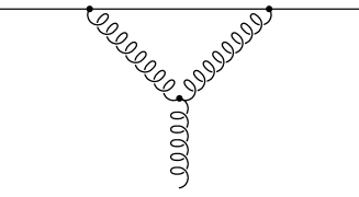
FIG. 1.: Non-abelian contribution to the one-loop vertex correction.

which gives radiative corrections to the form factors $F_{1}\left(q^{2}\right)$ and $F_{2}\left(q^{2}\right)$. In dimensional regularization, the diagram gives the $F_{1}$ and $F_{2}$ form factors as functions of the form $F_{1,2}(q^{2}/m^{2},\mu/m,\epsilon)$. The form factor can be expanded as a power series in $q^{2}/m^{2}$ at fixed $\epsilon$, followed by the limit $\epsilon\rightarrow 0$,

$$F_{1} = F_{1}\left(0\right)\left[{A_{0}\over\epsilon_{UV}}+{B_{0}\over\epsilon_{IR}}+\left(A_{0}+B_{0}\right)\log{\mu\over m}+D_{0}\right]$$ (22)

$$\qquad+q^{2}{dF_{1}\over d\,q^{2}}\left(0\right)\left[{A_{1}\over\epsilon_{UV}}+{B_{1}\over\epsilon_{IR}}+\left(A_{1}+B_{1}\right)\log{\mu\over m}+D_{1}\right]+\ldots,$$

and similarly for the $F_{2}$ form factor. It is conventional to label $\epsilon$ as either $\epsilon_{UV}$ or $\epsilon_{IR}$, depending on whether the integral is ultraviolet or infrared divergent. Ultraviolet divergences are cancelled by renormalization counterterms. Infrared divergences cancel when a physically measurable process is computed. Expanding the form factor in $q^{2}$ and then taking the limit $\epsilon\rightarrow 0$ gives an expression that is analytic in $q^{2}$, and misses terms which are non-analytic in $q^{2}$. The non-analytic terms are not needed for the calculation of the coefficients in the effective theory, since the effective Lagrangian is analytic in momentum. The coefficients of the effective Lagrangian are determined by computing (for example) the difference of $F_{1}$ in the full theory and effective theories. The non-analytic terms in $F_{1}$ cancel in the difference, and the analytic terms determine the unknown parameters $c_{F}\ldots c_{B2}$ in the effective Lagrangian.

Loop diagrams in HQET are functions $F(\{p\},\mu,\epsilon)$ times powers of the coefficients $c_{i}$ in the effective Lagrangian, where $\{p\}$ are the external momenta. All on-shell loop graphs vanish when expanded in powers of $p$, followed by $\epsilon\rightarrow 0$. This is because the coefficient of any power of $p$ is a dimensionally regulated integral of the form

$$\int{d^{d}\,k\over\left(2\pi\right)^{d}}f\left(k^{2},k\cdot v\right).$$ (23)

There is no dimensionful parameter in the integrand, so the integral vanishes. The matching condition is then trivial: one takes Eq. (22), and throws away the $1/\epsilon$ terms to obtain the difference of the graph in the full and effective theory. All the $1/\epsilon$ terms in the difference are ultraviolet divergences (which are cancelled by renormalization counterterms), since there are no infrared divergences in matching conditions. To see this more explicitly, one can evaluate integrals such as Eq. (23) by breaking them up into the sum of two integrals, one only ultraviolet divergent, and the other only infrared divergent. For example,

$$\int{d^{d}\,k\over\left(2\pi\right)^{d}}{1\over k^{4}}=\int{d^{d}\,k\over\left(2\pi\right)^{d}}\left[{1\over k^{2}\left(k^{2}+m^{2}\right)}+{m^{2}\over k^{4}\left(k^{2}+m^{2}\right)}\right]={1\over 16\pi^{2}}\left[{1\over\epsilon_{UV}}-{1\over\epsilon_{IR}}\right]=0,$$ (24)

since $\epsilon_{UV}=\epsilon_{IR}=\epsilon$. A given quantity in the effective theory is of the form

$$A_{\rm eff}\left({1\over\epsilon_{UV}}-{1\over\epsilon_{IR}}\right).$$ (25)

There can be no finite parts (the analogs of the $\left(A+B\right)\log\mu/m$ and $D$ terms in Eq. (22)), since the net integral is zero. A typical matching condition is of the form

$${\rm graphs\ in\ full\ theory}={\rm graphs\ in\ effective\ theory}+c_{i},$$ (26)

where $c_{i}$ is a coefficient in the effective Lagrangian. Using Eq. (22) and Eq. (25), the matching condition can be written as

$${B\over\epsilon_{IR}}+\left(A+B\right)\log{\mu\over m}+D=-A_{\rm eff}{1\over\epsilon_{IR}}+c_{i}.$$ (27)

The $1/\epsilon_{UV}$ terms are cancelled by the renormalization counterterms in the full and effective theories, respectively. The coefficients in the effective Lagrangian have no infrared divergences. Thus $B=-A_{\rm eff}$, and

$$c_{i}=\left(A+B\right)\log{\mu\over m}+D,$$ (28)

i.e. $c_{i}$ is obtained from Eq. (22) by keeping the finite pieces, and omitting the $1/\epsilon_{UV}$ and $1/\epsilon_{IR}$ terms.

The coefficients of the $Q^{\dagger}\left({{\bf D}^{2}/2m}\right)Q$ and $Q^{\dagger}\left({{\bf D}^{4}/8m^{3}}\right)Q$ are fixed by the dispersion relation $E^{2}=p^{2}+m^{2}$ of QCD, $c_{2}=c_{4}=1$. The other terms, which all contain at least one power of the gauge field $A^{\mu}$, are obtained by computing the one-loop $Q^{\dagger}QA$ on-shell scattering amplitude. The wave-function renormalization graph Fig. 2

FIG. 2.: One-loop wavefunction renormalization.

and the vertex correction Fig. 3

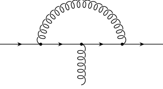
FIG. 3.: Abelian one-loop vertex correction.

can be found in many textbooks on quantum field theory [12]. In dimensional regularization, one finds that the wave function graph is

$$-i\Sigma\left(p\right) = -iC_{2}\left(Q\right){\alpha_{s}\over 4\pi}\left(A\left(p^{2}\right)m+B\left(p^{2}\right){\hbox to0.0pt{$p$\hss}/}\right)$$ (29)

$$A\left(p^{2}\right) = \int_{0}^{1}dx\ \Gamma\left(\epsilon/2\right)\left(4-\epsilon\right)\left[m^{2}x-p^{2}x(1-x)\right]^{-\epsilon/2}$$ (30)

$$B\left(p^{2}\right) = -\int_{0}^{1}dx\ \Gamma\left(\epsilon/2\right)\left(2-\epsilon\right)\left(1-x\right)\left[m^{2}x-p^{2}x(1-x)\right]^{-\epsilon/2}$$ (31)

where

$$C_{2}\left(Q\right)=T^{a}T^{a}={4\over 3}$$

is the Casimir of the quark representation. The on-shell wavefunction renormalization correction is

$$\delta Z = -C_{2}\left(Q\right){\alpha_{s}\over 4\pi}\left[B\left(m^{2}\right)+2m^{2}\left({\partial A\over\partial p^{2}}+{\partial B\over\partial p^{2}}\right)_{p^{2}=m^{2}}\right]$$ (32)

$$= C_{2}\left(Q\right){\alpha_{s}\over\pi}\left[{1\over 2\epsilon_{UV}}+{1\over\epsilon_{IR}}+1-{3\over 2}\log{m\over\mu}\right].$$ (33)

The on-shell vertex correction Fig. 3 can be expressed in terms of the form-factors $F_{1}$ and $F_{2}$,

$$-igT^{a}\ \bar{u}\left(p^{\prime}\right)\left[F_{1}\left(q^{2}\right)\gamma^{\mu}+iF_{2}\left(q^{2}\right){\sigma^{\mu\nu}q_{\nu}\over 2m}\right]u\left(p\right),$$ (34)

where $q=p^{\prime}-p$. The form factors are

$$F_{1}^{(V)}\left(q^{2}\right) = {\alpha\over 2\pi}\left(C_{2}\left(Q\right)-{1\over 2}C_{2}\left(ad\right)\right)\Biggl{[}{1\over\epsilon_{UV}}+{1\over\epsilon_{IR}}\left(2-{q^{2}\over m^{2}}\right)I\left(q^{2}/m^{2}\right)$$ (36)

$$+\left(3-{q^{2}\over m^{2}}\right)I\left(q^{2}/m^{2}\right)-{1\over 2}J\left(q^{2}/m^{2}\right)-\left(1-{q^{2}\over 2m^{2}}\right)K\left(q^{2}/m^{2}\right)-1\Biggr{]}$$

and

$$F_{2}^{(V)}\left(q^{2}\right)={\alpha\over 2\pi}\left(C_{2}\left(Q\right)-{1\over 2}C_{2}\left(ad\right)\right)I\left(q^{2}/m^{2}\right).$$ (37)

where

$$I\left(q^{2}/m^{2}\right)=\int_{0}^{1}dx\ {m^{2}\over m^{2}-q^{2}x(1-x)}$$ (38)

$$J\left(q^{2}/m^{2}\right)=\int_{0}^{1}dx\ \log{m^{2}-q^{2}x(1-x)\over\mu^{2}}$$ (39)

$$K\left(q^{2}/m^{2}\right)=\int_{0}^{1}dx\ {m^{2}\over m^{2}-q^{2}x(1-x)}\log{m^{2}-q^{2}x(1-x)\over\mu^{2}},$$ (40)

and

$$C_{2}\left(ad\right)=3$$

is the Casimir of the adjoint representation. Expanding to order $q^{2}/m^{2}$ gives

$$F_{1}^{(V)} = {\alpha\over\pi}\left(C_{2}\left(Q\right)-{1\over 2}C_{2}\left(ad\right)\right)\left[{1\over 2\epsilon_{UV}}+{1\over\epsilon_{IR}}+1-{3\over 2}\log{m\over\mu}+{q^{2}\over m^{2}}\left(-{1\over 3}{1\over\epsilon_{IR}}-{1\over 8}+{1\over 3}\log{m\over\mu}\right)\right],$$ (41)

$$F_{2}^{(V)} = {\alpha\over\pi}\left(C_{2}\left(Q\right)-{1\over 2}C_{2}\left(ad\right)\right)\left[{1\over 2}+{q^{2}\over 12m^{2}}\right].$$ (42)

The final diagram is the non-abelian vertex correction Fig. 1. This is computed in background field Feynman gauge, which preserves gauge invariance. The resulting diagram can also be evaluated in terms of the $F_{1}$ and $F_{2}$ form-factors,

$$F_{1}^{(g)} = {\alpha_{s}\over 8\pi}C_{2}\left(ad\right)\int_{0}^{1}dx\int_{0}^{1-x}dy\Biggl{\{}-\Gamma\left(1+\epsilon/2\right)\Bigl{[}2q^{2}\left(x+y\right)$$ (45)

$$+2m^{2}\left(1-x-y\right)\left(2\left(x+y\right)+\left(4-\epsilon\right)\left(1-x-y\right)\right)\Bigr{]}\left(m^{2}\left(x+y-1\right)^{2}-q^{2}xy\right)^{-1-\epsilon/2}$$

$$\qquad+\left(2-\epsilon\right)\Gamma\left(\epsilon/2\right)\left(m^{2}\left(x+y-1\right)^{2}-q^{2}xy\right)^{-\epsilon/2}\Biggr{\}}$$

$$= {\alpha_{s}\over 8\pi}C_{2}\left(ad\right)\left[{2\over\epsilon_{UV}}+{4\over\epsilon_{IR}}+4-6\log{m\over\mu}+{q^{2}\over m^{2}}\left(-{3\over\epsilon_{IR}}-1+3\log{m\over\mu}\right)+\ldots\right],$$ (46)

$$F_{2}^{(g)} = -{\alpha_{s}\over 4\pi}C_{2}\left(ad\right)m^{2}\Gamma\left(1+\epsilon/2\right)\int_{0}^{1}dx\int_{0}^{1-x}dy\left(1-x-y\right)$$ (48)

$$\qquad\times\left(\epsilon+\left(2-\epsilon\right)\left(x+y\right)\right)\left(m^{2}\left(x+y-1\right)^{2}-q^{2}xy\right)^{-1-\epsilon/2}$$

$$= {\alpha_{s}\over 8\pi}C_{2}\left(ad\right)\left[{4\over\epsilon_{IR}}+6-4\log{m\over\mu}+{q^{2}\over m^{2}}\left({4\over\epsilon_{IR}}+1-4\log{m\over\mu}\right)+\ldots\right].$$ (49)

The total on-shell form factors at one loop are given by

$$F_{1} = 1-\delta Z+F_{1}^{(V)}+F_{1}^{(g)}$$ (50)

$$= 1+{\alpha_{s}\over\pi}{q^{2}\over m^{2}}\left[\left(-{1\over 3\epsilon_{IR}}-{1\over 8}+{1\over 3}\log{m\over\mu}\right)C_{2}\left(Q\right)+\left(-{5\over 24\epsilon_{IR}}-{1\over 16}+{5\over 24}\log{m\over\mu}\right)C_{2}\left(ad\right)\right],$$ (51)

$$F_{2} = F_{2}^{(V)}+F_{2}^{(g)}$$ (52)

$$= {\alpha_{s}\over\pi}\left[{1\over 2}C_{2}\left(Q\right)+\left({1\over 2\epsilon_{IR}}+{1\over 2}-{1\over 2}\log{m\over\mu}\right)C_{2}\left(Q\right)\right]$$ (54)

$$\qquad+{\alpha_{s}\over\pi}{q^{2}\over m^{2}}\left[{1\over 12}C_{2}\left(Q\right)+\left({1\over 2\epsilon_{IR}}+{1\over 12}-{1\over 2}\log{m\over\mu}\right)C_{2}\left(ad\right)\right].$$

The total form-factor $F_{1}\left(0\right)$ is unity, since gauge invariance is preserved by the background field method.

The scattering amplitude for a low-momentum heavy quark off a background vector potential can be computed by expanding Eq. (34), and multiplying by $\sqrt{m/E}$ for the incoming and outgoing quarks. If ${\bf p}$ is the three-momentum of the incoming quark, ${\bf p}^{\prime}$ is the three-momentum of the outgoing quark, and ${\bf q=p^{\prime}-p}$, one finds that the effective interaction is

$$-igT^{a}\,u^{\dagger}_{NR}\left({\bf p}^{\prime}\right)\left[A^{0a}j^{0}-{\bf A}^{a}\cdot{\bf j}\right]u_{NR}\left({\bf p}\right),$$ (55)

where

$$j^{0}=F_{1}\left(q^{2}\right)\left\{1-{1\over 8m^{2}}\left|{\bf q}\right|^{2}+{i\over 4m^{2}}{\bf\mbox{\boldmath$\sigma$}\cdot\left(p^{\prime}\times p\right)}\right\}+F_{2}\left(q^{2}\right)\left\{-{1\over 4m^{2}}\left|{\bf q}\right|^{2}+{i\over 2m^{2}}{\bf\mbox{\boldmath$\sigma$}\cdot\left(p^{\prime}\times p\right)}\right\},$$ (56)

and

$${\bf j} = F_{1}\left(q^{2}\right)\Biggl{\{}{1\over 2m}\left({\bf p+p^{\prime}}\right)+{i\over 2m}{\bf\mbox{\boldmath$\sigma$}\times q}-{i\over 8m^{3}}\left(\left|{\bf p}\right|^{2}+\left|{\bf p^{\prime}}\right|^{2}\right){\bf\mbox{\boldmath$\sigma$}\times q}$$ (60)

$$-{i\over 16m^{3}}\left(\left|{\bf p^{\prime}}\right|^{2}-\left|{\bf p}\right|^{2}\right){\bf\mbox{\boldmath$\sigma$}\times\left(p+p^{\prime}\right)}-{1\over 8m^{3}}\left(\left|{\bf p^{\prime}}\right|^{2}+\left|{\bf p}\right|^{2}\right){\bf\left(p+p^{\prime}\right)}-{1\over 16m^{3}}\left(\left|{\bf p^{\prime}}\right|^{2}-\left|{\bf p}\right|^{2}\right){\bf q}\Biggr{\}}$$

$$+F_{2}\left(q^{2}\right)\Biggl{\{}{i\over 2m}{\bf\mbox{\boldmath$\sigma$}\times q}-{i\over 16m^{3}}\left|{\bf q}\right|^{2}{\bf\mbox{\boldmath$\sigma$}\times q}-{1\over 16m^{3}}\left|{\bf q}\right|^{2}{\bf\left(p^{\prime}+p\right)}$$

$$-{1\over 16m^{3}}\left(\left|{\bf p^{\prime}}\right|^{2}-\left|{\bf p}\right|^{2}\right){\bf q}-{i\over 8m^{3}}\left(\left|{\bf p^{\prime}}\right|^{2}-\left|{\bf p}\right|^{2}\right){\bf\mbox{\boldmath$\sigma$}\times\left(p^{\prime}+p\right)}+{i\over 8m^{3}}{\bf\mbox{\boldmath$\sigma$}\cdot\left(p^{\prime}+p\right)}\left({\bf p^{\prime}\times p}\right)\Biggr{\}}.$$

Comparing Eqs. (56,60) with the scattering amplitude in the effective theory from the Lagrangian Eq. (6) gives

$$c_{F} = F_{1}+F_{2}$$ (61)

$$c_{D} = F_{1}+2F_{2}+8F_{1}^{\prime}$$ (62)

$$c_{S} = F_{1}+2F_{2}$$ (63)

$$c_{W1} = F_{1}+{1\over 2}F_{2}+4F_{1}^{\prime}+4F_{2}^{\prime}$$ (64)

$$c_{W2} = {1\over 2}F_{2}+4F_{1}^{\prime}+4F_{2}^{\prime}$$ (65)

$$c_{p^{\prime}p} = F_{2}$$ (66)

$$c_{M} = -{1\over 2}F_{2}-4F_{1}^{\prime}$$ (67)

where

$$F_{i}\equiv F_{i}\left(0\right),\qquad F_{i}^{\prime}\equiv\left.{dF_{i}\over d\left(q^{2}/m^{2}\right)}\right|_{q^{2}=0}$$ (68)

Note that the nine parameters (including $c_{2}$ and $c_{4}$) in the effective Lagrangian Eq. (6) are determined in terms of only three independent constants, $F_{2}$, $F_{1}^{\prime}$, and $F_{2}^{\prime}$, since $F_{1}=1$. Reparametrization invariance [14] gives six linear relations among the coefficients. This will be discussed in more detail in the next section.

The explicit expressions for the coefficients are obtained using Eqs. (50,52):

$$c_{F} = 1+{\alpha\over\pi}\left[{1\over 2}C_{2}\left(Q\right)+\left({1\over 2}-{1\over 2}\log{m\over\mu}\right)C_{2}\left(ad\right)\right]$$ (69)

$$c_{D} = 1+{\alpha\over\pi}\left[\left({8\over 3}\log{m\over\mu}\right)C_{2}\left(Q\right)+\left({1\over 2}+{2\over 3}\log{m\over\mu}\right)C_{2}\left(ad\right)\right]$$ (70)

$$c_{S} = 1+{\alpha\over\pi}\left[C_{2}\left(Q\right)+\left(1-\log{m\over\mu}\right)C_{2}\left(ad\right)\right]$$ (71)

$$c_{W1} = 1+{\alpha\over\pi}\left[\left({1\over 12}+{4\over 3}\log{m\over\mu}\right)C_{2}\left(Q\right)+\left({1\over 3}-{17\over 12}\log{m\over\mu}\right)C_{2}\left(ad\right)\right]$$ (72)

$$c_{W2} = {\alpha\over\pi}\left[\left({1\over 12}+{4\over 3}\log{m\over\mu}\right)C_{2}\left(Q\right)+\left({1\over 3}-{17\over 12}\log{m\over\mu}\right)C_{2}\left(ad\right)\right]$$ (73)

$$c_{p^{\prime}p} = {\alpha\over\pi}\left[{1\over 2}C_{2}\left(Q\right)+\left({1\over 2}-{1\over 2}\log{m\over\mu}\right)C_{2}\left(ad\right)\right]$$ (74)

$$c_{M} = {\alpha\over\pi}\left[\left({1\over 4}-{4\over 3}\log{m\over\mu}\right)C_{2}\left(Q\right)-\left({7\over 12}\log{m\over\mu}\right)C_{2}\left(ad\right)\right]$$ (75)

The results for NRQED can be obtained by setting $C_{2}\left(ad\right)=0$ and $C_{2}\left(Q\right)=1$, and agree with those found in [9], with the replacement

$$\log\mu\rightarrow\log 2\Lambda-{5\over 6}$$ (76)

The difference in finite parts is because the NRQED integrals were evaluated in Ref. [9] using a momentum space cutoff, instead of using dimensional regularization. The results for the $1/m$ operators agree with known results for HQET [4, 5]. The $1/m^{2}$ matching conditions at tree-level, and the $\mu$ dependence at one-loop also agree with known results [6, 7, 8]. Note that $c_{F}$ is independent of $\mu$ in QED. This is easy to see if one computes the renormalization of the magnetic moment operator in the effective theory in Coulomb gauge, in which all transverse photon interactions are suppressed by $1/m$.

The discussion so far has concentrated on the fermion part of the effective Lagrangian. There is, in addition, the pure gauge field part of the effective action. The one-loop correction to the gluon propagator is shown in Figs. (4)

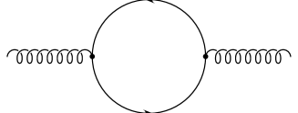
FIG. 4.: Quark contribution to the vacuum polarization.

and (5).

FIG. 5.: Gluon contribution to the vacuum polarization.

The gluon diagram is the same in QCD and in HQET, so the one-loop matching condition is from the quark vacuum polarization diagram. This gives the effective action [15, 16, 17]

$${\cal L}=-{1\over 4}d_{1}G_{\mu\nu}^{A}G^{A\mu\nu}+{d_{2}\over m^{2}}G_{\mu\nu}^{A}D^{2}G^{A\mu\nu}+{d_{3}\over m^{2}}gf_{ABC}G_{\mu\nu}^{A}G_{\mu\alpha}^{B}G_{\nu\alpha}^{C}+{\cal O}\left({1\over m^{4}}\right),$$ (77)

with

$$d_{1} = 1-{\alpha\over 3\pi}T\left(Q\right)\log m^{2}/\mu^{2},$$ (78)

$$d_{2} = {\alpha\over 60\pi}T\left(Q\right),$$ (79)

$$d_{3} = {13\alpha\over 360\pi}T\left(Q\right),$$ (80)

where

$$T\left(Q\right)=1/2$$

is the index of the quark representation. The identity

$$0=\int 2\ D^{\mu}\,G_{\mu\alpha}^{A}\,D_{\nu}\,G^{\nu\alpha A}+2\ g\,f_{ABC}\,G_{\mu\nu}^{A}G_{\mu\alpha}^{B}G_{\nu\alpha}^{C}+G_{\mu\nu}^{A}\,D^{2}\,G^{A\mu\nu}$$

has been used to eliminate $D^{\mu}\,G_{\mu\alpha}^{A}\,D_{\nu}\,G^{\nu\alpha A}$ from Eq. (77).

V Reparametrization Invariance

The coefficients of operators in the HQET Lagrangian are constrained by reparametrization invariance [14]. The reparametrization invariant spinor field $\Psi_{v}$ is given by

$$\Psi_{v}=\Lambda\left(w,v\right)\psi_{v},$$ (81)

where $\psi_{v}$ is the conventional heavy quark field that satisfies

$${\hbox to0.0pt{$v$\hss}/}\psi_{v}=\psi_{v},$$ (82)

$\Lambda(w,v)$ is the Lorentz transformation matrix

$$\Lambda\left(w,v\right)={1+{\hbox to0.0pt{$w$\hss}/}\ {\hbox to0.0pt{$v$\hss}/}\over\sqrt{2\left(1+w\cdot v\right)}},$$ (83)

and

$$w^{\mu}={v^{\mu}+iD^{\mu}/m\over\left|v^{\mu}+iD^{\mu}/m\right|}.$$ (84)

One needs to choose a particular operator ordering for the covariant derivatives; different orderings are related to each other by field redefinitions.

It is simplest to consider the consequences of reparametrization invariance when $D^{\mu}\rightarrow\partial^{\mu}$ in Eq. (81). Then there is no operator ordering ambiguity, and the field $\Psi_{v}$ can be written as

$$\Psi_{v} = \left[{1\over 2\sqrt{\left(m+i\partial\cdot v\right)^{2}+\left(i{\partial_{\perp}}\right)^{2}}\left(m+i\partial\cdot v+\sqrt{\left(m+i\partial\cdot v\right)^{2}+\left(i{\partial_{\perp}}\right)^{2}}\right)}\right]^{1/2}$$ (86)

$$\times\left[m++i\partial\cdot v+i{\hbox to0.0pt{$\partial$\hss}/}_{\perp}+\sqrt{\left(m+i\partial\cdot v\right)^{2}+\left(i{\partial_{\perp}}\right)^{2}}\right]\psi_{v},$$

where

$$\partial^{\mu}_{\perp}=\partial^{\mu}-v^{\mu}\ \partial\cdot v.$$ (87)

If one uses Eq. (86), replaces $\psi_{v}$ by the spinor $u_{NR}e^{-ip\cdot x}$, with $p^{2}=m^{2}$, $\gamma^{0}u_{NR}=u_{NR}$, $\bar{u}_{NR}^{\dagger}u_{NR}=1$, and $v=\left(1,0,0,0)\right)$, the field $\Psi_{v}$ reduces to the spinor $ue^{-ip\cdot x}$, that satisfies the Dirac equation ${\hbox to0.0pt{$p$\hss}/}u=mu$, and is normalized so that $\bar{u}u=1$. This shows that reparametrization invariance will determine the coefficients of the $1/m$ suppressed operators which are fixed by relativistic invariance.

The reparametrization invariant kinetic term is

$$\bar{\Psi}_{v}i{\hbox to0.0pt{$\partial$\hss}/}\,\Psi_{v}=\bar{\psi}_{v}\left[\sqrt{\left(m+i\partial\cdot v\right)^{2}+\left(i\partial_{\perp}\right)^{2}}-m\right]\psi_{v}.$$ (88)

This is not the same as the terms in the Lagrangian Eq. (6). The reparametrization invariant field Eq. (81) does not automatically produce a Lagrangian in the “standard” NRQCD form. However, one can convert Eq. (88) to this form by making a field redefinition,

$$\psi_{v}=\left[{\sqrt{\left(m+i\partial\cdot v\right)^{2}+\left(i\partial_{\perp}\right)^{2}}+m\over m+i\partial\cdot v+\sqrt{-\left(i\partial_{\perp}\right)^{2}+m^{2}}}\right]^{1/2}\psi_{v}^{\prime}$$ (89)

The kinetic energy term in the primed field is

$$\bar{\psi}_{v}^{\prime}\left[m+i\partial\cdot v-\sqrt{-\left(i\partial_{\perp}\right)^{2}+m^{2}}\right]\psi_{v}^{\prime}.$$ (90)

which when expanded gives Eq. (6) with $c_{2}=c_{4}=1$. Thus $c_{2}=c_{4}=1$ follows from reparametrization invariance. The transformation factor in Eq. (89) when applied to on-shell spinors (instead of fields) reduces to $\sqrt{m/E}$. This is the same as the flux factor for the incoming and outgoing particles which was included in Eq. (55).

To determine the constraints of reparametrization invariance on the effective Lagrangian, consider Eq. (86) with the gauge fields included, i.e. with $\partial\rightarrow D$. Expanding to order $1/m^{3}$ gives

$$\Psi_{v}=\left[1+A+{i{\,\raise 0.6458pt\hbox{/}\mkern-13.5muD}_{\perp}\over 2m}B\right]\psi_{v}$$ (91)

where

$$A = 1-{\left(iD_{\perp}\right)^{2}\over 8m^{2}}+{\left(iD_{\perp}\right)^{2}\left(iv\cdot D\right)\over 4m^{3}}$$ (92)

$$B = 1-{iv\cdot D\over m}-{3\left(iD_{\perp}\right)^{2}\over 8m^{2}}+{\left(iv\cdot D\right)^{2}\over m^{2}}.$$ (93)

A particular ordering has been chosen for the operators in Eq. (91). A different ordering gives an effective Lagrangian that is related by a field redefinition.

The most general reparametrization invariant Lagrangian is a linear combination of invariant terms, such as $\bar{\Psi}_{v}\left({\hbox to0.0pt{$v$\hss}/}+i\,\raise 0.6458pt\hbox{/}\mkern-13.5muD/m\right)\Psi_{v}$, $\bar{\Psi}_{v}\sigma^{\alpha\beta}G_{\alpha\beta}\Psi_{v}$, etc. The effective Lagrangian obtained in this way is not in the form Eq. (11), but it can be converted into that form by field redefinitions that preserve ${\hbox to0.0pt{$v$\hss}/}\psi_{v}=\psi_{v}$. One finds by a straightforward (but not very enlightening computation) that the effective Lagrangian is a linear combination of the invariant linear combinations

$$iv\cdot D+O_{2}+O_{4}+O_{F}+O_{D}+O_{S}+O_{W1},$$ (94)

$$2O_{F}+4O_{D}+4O_{S}+O_{W1}+O_{W2}+2O_{p^{\prime}p}-O_{M},$$ (95)

$$O_{W1}+O_{W2},$$ (96)

$$2O_{D}+O_{W1}+O_{W2}-O_{M},$$ (97)

$$O_{A1},\ O_{A2},\ O_{A3},\ O_{A4},\ O_{B1},\ O_{B2},$$ (98)

up to terms of order $1/m^{4}$. Here $O_{F}$, etc. are the operator coefficients of $c_{F}$, etc. in Eq. (11). The above linear combinations imply the constraints

$$c_{2} = 1,$$ (99)

$$c_{4} = 1,$$ (100)

$$c_{S} = 2c_{F}-1,$$ (101)

$$c_{W2} = c_{W1}-1,$$ (102)

$$c_{p^{\prime}p} = c_{F}-1,$$ (103)

$$2c_{M} = c_{F}-c_{D}.$$ (104)

which are satisfied by Eqs. (61),(69).

VI Conclusions

The HQET/NRQCD Lagrangian has been computed to one loop and order $1/m^{3}$, and has been shown to be reparametrization invariant to order $\alpha/m^{3}$. The original form of the NRQCD propagator Eq. (2) cannot be used to compute the effective Lagrangian by matching to QCD. Instead, one must treat the propagator as an infinite series, and resum the series after doing the loop integral. As a result, the matching computations for NRQCD and HQET are the same. It is straightforward to obtain the effective Lagrangian (in the one-quark sector) to higher orders in $1/m$ by expanding the form factors $F_{1,2}$ and the spinors in the computation of Eqs. (55),(56) to higher orders. No further Feynman graphs need to be evaluated.

REFERENCES

• [1] N. Isgur and M.B. Wise, Phys. Lett. B232 113 (1989); Phys. Lett. B237 527 (1990).
• [2] W.E. Caswell and G.P. Lepage, Phys. Lett. B167, 437 (1986).
• [3] G.T. Bodwin, E. Braaten, and G.P. Lepage, Phys.ย Rev.ย D51, 1125 (1995).
• [4] E. Eichten and B. Hill, Phys.ย Lett.ย B243, 427 (1990).
• [5] A.F.ย Falk, B.ย Grinstein, and M.E.ย Luke, Nucl.ย Phys.ย B357, 185 (1991).
• [6] C.ย Balzereit and T.ย Ohl, Phys.ย Lett.ย B386, 335 (1996).
• [7] C.ย Bauer, Diplom Thesis, Karlsruhe 1996 (unpublished).
• [8] B.ย Blok, J.G.ย Korner, D.ย Pirjol, and J.C.ย Rojas, hep-ph/9607233.
• [9] T.ย Kinoshita and M.ย Nio, Phys.ย Rev.ย D53, 4909 (1996).
• [10] C.ย Morningstar, Phys.ย Rev.ย D48, 2265 (1993), D50, 5902 (1994).
• [11] H.D.ย Politzer, Nucl.ย Phys. B172, 349 (1980).
• [12] See for example, S.ย Pokorski, Gauge Field Theories, Cambridge University Press, 1987.
• [13] M.E.ย Luke and A.V.ย Manohar, hep-ph/9610534.
• [14] M.E.ย Luke and A.V.ย Manohar, Phys.ย Lett.ย B286, 348 (1992).
• [15] P.ย Cho and E.H.ย Simmons, Phys.ย Rev.ย D51, 2360 (1995).
• [16] V.ย Novikov, M.ย Shifman, A.ย Vainshtein, and V.ย Zakharov, Fort.ย Phys.ย 32, 585 (1984).
• [17] S.ย Balk, J.G.ย Korner, and D.ย Pirjol, Nucl.ย Phys.ย B428, 499 (1994).