FERMILAB–PUB–96/455–T NORDITA–96–81–P hep-ph/9701238

Use and Misuse of QCD Sum Rules in Heavy-to-light Transitions: the Decay $B\to\rho e\nu$ Reexamined

Patricia Ball Fermi National Accelerator Laboratory, P.O. Box 500, Batavia, IL 60510, USA

V.M. Braun
NORDITA, Blegdamsvej 17, DK–2100 Copenhagen, Denmark

Abstract:
The existing calculations of the form factors describing the decay $B\to\rho e\nu$ from QCD sum rules have yielded conflicting results at small values of the invariant mass squared of the lepton pair. We demonstrate that the disagreement originates from the failure of the short-distance expansion to describe the $\rho$ meson distribution amplitude in the region where almost the whole momentum is carried by one of the constituents. This limits the applicability of QCD sum rules based on the short-distance expansion of a three-point correlation function to heavy-to-light transitions and calls for an expansion around the light-cone, as realized in the light-cone sum rule approach. We derive and update light-cone sum rules for all the semileptonic form factors, using recent results on the $\rho$ meson distribution amplitudes. The results are presented in detail together with a careful analysis of the uncertainties, including estimates of higher-twist effects, and compared to lattice calculations and recent CLEO measurements. We also derive a set of “improved” three-point sum rules, in which some of the problems of the short-distance expansion are avoided and whose results agree to good accuracy with those from light-cone sum rules.
Submitted to Physical Review D

1 Introduction

The interest in the study of semileptonic $B$ decays is mainly due to their importance in determining the CKM matrix elements $|V_{cb}|$ and $|V_{ub}|$. Whereas the theoretical analysis of both exclusive and inclusive $b\to c$ transitions is decisively simplified by an expansion in the inverse heavy quark mass, this method is of only little use in $b\to u$ transitions. This is essentially due to the fact that in inclusive channels experimental observation is possible only in a small region of phase-space beyond the kinematical threshold for charm production, in which the hadron multiplicity is small. Thus, since the theoretical description of inclusive decays is essentially based on a parton-model picture, it is not very predictive in the experimentally accessible range, cf. [1]. It is therefore rather the exclusive decay channels, in particular $B\to\pi\ell\nu$ and $B\to\rho\ell\nu$, that seem to be more suitable for obtaining reliable information on $|V_{ub}|$. The CLEO collaboration has recently presented first experimental results of these branching ratios [2], which, however, are model-dependent.

The decay $B\to\pi\ell\nu$ has been tackled by several authors using a number of different approaches, in particular QCD sum rules [3, 4, 5, 6] and simulations on the lattice [7, 8, 9, 10]; the results are in reasonable agreement. The situation is, however, not that favourable in the $B\to\rho$ channel. Although here the same methods were applied, the resulting predictions for the decay rates are quite different. To illustrate the origin of the problem, let us first introduce the relevant observables: the hadronic matrix element determining the $B\to\rho$ weak transition is

$$\langle\rho,\lambda|(V-A)_{\mu}|B\rangle = -i(m_{B}+m_{\rho})A_{1}(t)\epsilon_{\mu}^{*(\lambda)}+\frac{iA_{2}(t)}{m_{B}+m_{\rho}}(\epsilon^{*(\lambda)}p_{B})(p_{B}+p_{\rho})_{\mu}$$ (1.1)

$${}+\frac{iA_{3}(t)}{m_{B}+m_{\rho}}(\epsilon^{*(\lambda)}p_{B})(p_{B}-p_{\rho})_{\mu}+\frac{2V(t)}{m_{B}+m_{\rho}}\epsilon_{\mu}^{\phantom{\mu}\alpha\beta\gamma}\epsilon_{\alpha}^{*(\lambda)}p_{B\beta}p_{\rho\gamma},\makebox[22.76228pt]{}$$

where the four form factors $A_{1,2,3}$ and $V$ depend on the momentum transfer $t=(p_{B}-p_{\rho})^{2}$ to the leptons; in the limit of vanishing lepton mass $A_{3}$ does not contribute to the semileptonic decay rate and will not be considered in this paper. $\lambda$ is the polarization of the $\rho$, $t$ takes values between 0 and 20.3 GeV². It is precisely this large range of relevant $t$ that renders the theoretical description of the form factors in (1.1) so difficult. Most quark model calculations rely essentially on the pole-dominance picture [11] or on a nonrelativistic description, which yields an exponential increase of the form factors with $t$ [12], which was softened in an updated version of the model, Ref. [13]. Lattice calculations are up to now limited to small momenta of the final state $\rho$ [7, 8, 14] and/or require extrapolations in the heavy quark mass. For $B\to\pi\ell\nu$, the possibility to restrict the functional $t$ dependence of the single relevant form factor from unitarity with the supplementary input of available lattice data at large $t$ was investigated in [10], but this method is presently not very predictive in the $\rho$ channel, see [15].

To date, only lattice simulations and QCD sum rules seem to be apt to predict the $t$ dependence in nearly the whole physical region. QCD sum rules provide a consistent description of semileptonic $D$ decays [16] and of the $B\to\pi$ semileptonic form factor [3, 4, 5, 6]. However, there exist conflicting predictions from different types of QCD sum rules for $B\to\rho$ decays, which differ by a factor 2 in the form factors at maximum recoil [5, 17]. The aim of this paper is to clarify the origin of this difference and to give updated predictions for the form factors, which include in particular recently gained information on the structure of $\rho$ mesons probed at large momentum transfer [18].

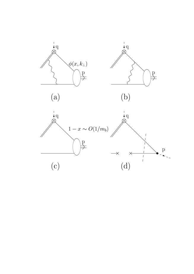
Figure 1: “Hard” (a,b) and “soft” (c) contributions to the decay form factor. (d): modelling of the soft contribution in the QCD sum rule approach. See explanation in the text.

At large recoil, the light quark originating from the weak decay carries a large energy of order $m_{b}/2$ and has to transfer it to the soft cloud to recombine to the final state hadron. The probability of such a recombination depends on the parton content of both the $B$ meson and the light meson, the valence configuration with the minimum number of Fock constituents being dominant. The valence quark configuration is characterized by the wave function $\phi(x,k_{\perp})$ depending on the momentum fraction $x$ carried by the quark and on its transverse momentum $k_{\perp}$. There exist two different mechanisms for the valence quark contribution to the transition form factor. The first one is the hard rescattering mechanism pictured in Figs. 1(a,b), which requires that the recoiling and spectator quarks are at small transverse separations. In this case the large momentum is transferred by an exchange of a hard gluon with virtuality $k^{2}\sim O(m_{b})$. This contribution is perturbatively calculable in terms of the Bethe-Salpeter wave functions at small ($\sim 1/m_{b}$) transverse separations, or distribution amplitudes:

$$\phi(x)=\int^{k_{\perp}^{2}\sim m_{b}}dk_{\perp}^{2}\phi(x,k_{\perp}).$$ (1.2)

The second mechanism is the soft contribution, shown schematically in Fig. 1(c). The idea is that hard gluon exchange is not necessary, provided one picks up an “end-point” configuration with almost all momentum $1-x\sim O(1/m_{b})$ carried by one constituent. Since at large scales $\phi(x)\sim 1-x$ [19], the overlap integral is of order $\int_{1-O(1/m_{b})}^{1}dx\,\phi(x)\sim O(1/m_{b}^{2})$. An additional factor $m_{b}^{1/2}$ comes from the normalization of the heavy initial state, so that the final scaling law for the soft contribution to the form factor at large recoil is $1/m^{3/2}_{b}$ [20, 17, 21]. Note that the transverse quark-antiquark separation is not constrained in this case, which implies that the soft contribution is sensitive to long-distance dynamics. To calculate the soft contribution one needs to know the wave function as a function of the transverse separation; the simpler distribution amplitude is not enough.

Hard exclusive processes involving light hadrons receive the same two types of contributions. There is a major difference, however, in that for light hadrons the soft contribution is suppressed by a power of the large momentum (i.e. it is of higher-twist), while for heavy meson decays both soft and hard contributions turn out to be of the same power in the heavy quark mass [20, 17, 21]. As a result, the soft (end-point) contribution is expected to be large and requires quantitative evaluation.

It was suggested [21] that Sudakov-type perturbative corrections cut off contributions of large transverse separations so that the soft contributions might be suppressed. This suppression eventually eliminates the soft contribution for very large $m_{b}$. At the realistic values $m_{b}\approx 5\,$GeV, however, it is unlikely that calculations of this type can provide a quantitative description. Indeed, the existing estimates of “hard” contributions typically fall short of realistic values of the form factors from model calculations.

Here the QCD sum rules method enters the stage and suggests a nonperturbative technique to estimate the necessary convolution integral without explicit knowledge of the wave functions.

There exist two different types of QCD sum rules, which, being similar in spirit, differ in the treatment of the light hadron in the final state. This is illustrated in Figs. 1(c,d).

The “traditional” sum rules avoid introducing wave functions altogether by considering a three-point correlation function with a suitable interpolating current and use dispersion relations to extract the contribution of the ground state. The most important nonperturbative effect is then described by the diagram in Fig. 1(d), where the light quark is soft and interacts with the nonperturbative QCD vacuum, forming the so-called quark condensate. Since quarks in a condensate have zero momentum, it is clear that this diagram yields a contribution to the distribution amplitude that is naively proportional to $\delta(1-x)$ and remains unsuppressed for $m_{b}\to\infty$. This obviously violates the power counting discussed above. The contradiction must be resolved by including the contributions of higher-order condensates to the sum rules and subtracting the contribution of excited states. The suppression of the end-point region $x\to 1$, which is strictly required by QCD, is thus expected to hold as a numerical cancellation between different contributions, which becomes the more delicate (and requires more fine-tuning) the more $m_{b}$ increases. For $m_{b}\approx 5\,$GeV a suppression of the quark condensate contribution by a factor $\sim 1\,$GeV${}^{2}/m_{b}^{2}\sim 1/25$ is required. This explains why the traditional three-point sum rules become unreliable.

The light-cone sum rules avoid this problem by rearranging the calculation in such a way that nonperturbative effects like the interaction with the quark condensate are included in the nonperturbative hadron distribution amplitudes, estimated using additional sum rules [24]. These additional sum rules are written for integrated characteristics of the distribution amplitudes like moments, and the correct asymptotic behaviour at the end-points is included by construction.

The contribution of a single leading-twist distribution amplitude incorporates an infinite set of contributions of condensates of increasing dimension in the standard approach, at the cost of retaining pieces with the largest Lorentz spin (lowest twist) only. The remaining pieces of condensate contributions are organized in a similar way in the contributions of higher-twist distribution amplitudes.

The premium for this rearrangement is that light-cone sum rules have the correct asymptotic behaviour in the heavy quark limit, but the snag is that the present knowledge of higher-twist distribution amplitudes is incomplete, so that not all known nonperturbative corrections of the standard approach can be included. One should expect that these two approaches provide complimentary descriptions of $B$ decays, with their own advantages and disadvantages.

Note that the problem with three-point sum rules originates from the constraint of the distribution amplitude convolution integral to the end-point region; this makes the answer very sensitive to the precise shape of the distribution amplitude rather than its integrated characteristics. For the decay form factors at small recoil there is no such restriction, and the classical QCD sum rule concept of taking into account nonperturbative effects as the contributions of long-wave vacuum fluctuations (condensates) classified by their dimension is adequate. Thus, at small recoil, both types of the sum rules should yield similar results and the spread of their predictions characterizes the accuracy of the method. At large recoil one should rely on the light-cone sum rules.

It is worthwhile to add that contributions of hard rescattering can be consistently included as radiative corrections to the sum rules. Their inclusion is technically challenging, but does not pose a problem of principle.

Our paper is organized as follows. In Sec. 2 we introduce the two different types of QCD sum rules. In Sec. 3 we then analyse and explain the discrepancy in $B\to\rho$ transitions, paying special attention to the rearrangement of quark and mixed condensate contributions within the light-cone expansion. We also estimate higher-twist contributions to $A_{1}$. In Sec. 4 we discuss shortly the quark mass dependence and the heavy quark limit. Section 5 contains our final predictions for form factors, spectra and decay rates of $B\to\rho e\nu$, Sec. 6 a summary and the discussion of the results. More technical issues are delegated to appendices.

2 Three-Point vs. Light-Cone Sum Rules

In this section we discuss the two different types of QCD sum rules that have been used in the literature to calculate heavy-to-light meson decays.

2.1 Three-Point Sum Rules

The – comparatively speaking – “traditional” approach towards transition matrix elements is by calculating a three-point (“3pt” in the following) correlation function. Specifically, for $B\to\rho$ one considers

$$\Gamma^{\mu\nu} = i^{2}\!\!\int d^{4}x\,d^{4}y\,e^{-ip_{B}x+ip_{\rho}y}\,\langle 0|Tj_{\rho}^{\nu}(y)(V-A)^{\mu}(0)j_{B}^{\dagger}(x)|0\rangle$$ (2.1)

$$= ig^{\mu\nu}\Gamma_{0}-i(p_{B}+p_{\rho})^{\mu}p_{B}^{\nu}\Gamma_{+}-\epsilon^{\mu\nu}_{\phantom{\mu\nu}\rho\sigma}p_{B}^{\rho}p_{\rho}^{\sigma}\Gamma_{V}+\dots$$

Here $(V-A)_{\mu}=\bar{u}\gamma_{\mu}(1-\gamma_{5})b$ is the weak current mediating the $b\to u$ transition, $j_{B}=\bar{q}i\gamma_{5}b$ is the interpolating field for the pseudoscalar $B$ meson, and $j_{\rho}^{\nu}=\bar{q}\gamma^{\nu}u$ the interpolating field for the $\rho$ meson. In (2.1) we have given explicitly only those Lorentz structures that are relevant for the semileptonic decay channel, the others are suppressed.

The method of QCD sum rules consists – in principle – in performing on the one hand a QCD calculation of $\Gamma^{\mu\nu}$ in the not so deep Euclidean region $p_{\rho}^{2}\sim p_{B}^{2}-m_{b}^{2}\sim O(1\,$GeV²), writing it on the other hand as (double) dispersion relation over the physical cut and equating both expressions. It was the idea of Shifman, Vainshtein and Zakharov [25] to complement the purely perturbative calculation of $\Gamma^{\mu\nu}$ by nonperturbative terms in form of vacuum matrix elements of gauge-invariant local operators, the condensates. The method proved surprisingly successful in describing various hadronic matrix elements in terms of a handful of input parameters, as is testified by the immense number of publications in the field.

The traditional approach by SVZ appeals to Wilson’s operator product expansion (OPE), which is the expansion of a T-product of currents at short distances in terms of local operators. In that way one obtains for the invariants $\Gamma$ in (2.1):

$$\Gamma(p_{B}^{2},p_{\rho}^{2},t)=\sum_{n}\Gamma^{(n)}(p_{B}^{2},p_{\rho}^{2},t)\langle\,0\,|\,{\cal O}_{n}\,|\,0\,\rangle$$ (2.2)

with the condensates $\langle\,0\,|\,{\cal O}_{n}\,|\,0\,\rangle$. In most applications one takes into account condensates up to dimension 6. $\Gamma$ can also be expressed as a dispersion relation over the physical singularities:

$$\Gamma=\int\!\!ds_{B}\,ds_{\rho}\,\frac{\rho^{\rm phys}(s_{B},s_{\rho},t)}{(s_{B}-p_{B}^{2})(s_{\rho}-p_{\rho}^{2})}+{\rm subtractions}.$$ (2.3)

Usually one is interested only in the properties of the ground state, which has to be extracted from the sum over all states. For this, one writes

$$\rho^{\rm phys}=\rho^{\rm ground\ state}+\rho^{\rm cont}$$ (2.4)

and approximates the unknown contribution of the continuum by the perturbative spectral function above some “continuum-thresholds” $s_{0}^{B}$ and $s_{0}^{\rho}$, such that

$$\rho^{\rm cont}\simeq\rho^{\rm pert}\{1-\Theta(s_{B}^{0}-s_{B})\,\Theta(s_{\rho}^{0}-s_{\rho})\},$$ (2.5)

where the “$\simeq$” indicates that smearing over a sufficiently large interval is implied. The sum rule is then obtained by equating (2.2) and (2.3) and subtracting from both sides the continuum contribution, i.e. in the above approximation the integral over the perturbative double spectral function above thresholds. In order to reduce the impact of this approximation on the final results as well as the error induced by truncating the series (2.2) after the first few terms, one subjects the sum rule to a Borel transformation. For an arbitrary function of Euclidean momentum, $f(P^{2})$ with $P^{2}=-p^{2}$, the transformation is defined by:

$$\hat{f}:=\widehat{B}_{P^{2}}(M^{2})\,f=\lim_{\begin{array}[]{c}\scriptstyle P^{2}\to\infty,N\to\infty\\[-2.84526pt] \scriptstyle P^{2}/N=M^{2}{\rm\ fixed}\end{array}}\frac{1}{N!}(-P^{2})^{N+1}\frac{d^{N+1}}{(dP^{2})^{N+1}}\,f,$$ (2.6)

where $M^{2}$ is the so-called Borel parameter. For a typical term in the OPE, the transformation yields

$$\widehat{B}_{P^{2}}(M^{2})\,\frac{1}{(p^{2}-m^{2})^{n}}=\frac{1}{(n-1)!}\,(-1)^{n}\,\frac{1}{(M^{2})^{n}}e^{-m^{2}/M^{2}}.$$ (2.7)

As condensates with large dimension get divided by correspondingly high powers of $(p^{2}-m^{2})$, their contributions to the sum rules get suppressed by factorials. In the dispersion integrals, $\rho^{\rm cont}$ gets exponentially suppressed relatively to the ground state contribution, which is just the desired effect.

Defining the couplings of the mesons to their interpolating fields by

$$\langle\,0|\,\bar{d}i\gamma_{5}b\,|\,\bar{B}^{0}\,\rangle=f_{B}\frac{m_{B}^{2}}{m_{b}}\,,\qquad\langle\,0\,|\,\bar{d}\gamma_{\nu}u\,|\,\rho^{+},\lambda\,\rangle=f_{\rho}m_{\rho}\epsilon^{(\lambda)}_{\nu},$$ (2.8)

we find the following sum rules for the form factors determining the semileptonic $B\to\rho$ transition:

$$A_{1}^{B\to\rho}(t) = \frac{m_{b}}{f_{B}f_{\rho}(m_{B}+m_{\rho})m_{B}^{2}m_{\rho}}\,\exp\left\{\frac{m_{B}^{2}}{M_{B}^{2}}+\frac{m_{\rho}^{2}}{M_{\rho}^{2}}\right\}M_{B}^{2}M_{\rho}^{2}\hat{\Gamma}_{0},$$ (2.9)

$$A_{2}^{B\to\rho}(t) = \frac{m_{b}(m_{B}+m_{\rho})}{f_{B}f_{\rho}m_{B}^{2}m_{\rho}}\,\exp\left\{\frac{m_{B}^{2}}{M_{B}^{2}}+\frac{m_{\rho}^{2}}{M_{\rho}^{2}}\right\}M_{B}^{2}M_{\rho}^{2}\hat{\Gamma}_{+},$$ (2.10)

$$V^{B\to\rho}(t) = \frac{m_{b}(m_{B}+m_{\rho})}{2f_{B}f_{\rho}m_{B}^{2}m_{\rho}}\,\exp\left\{\frac{m_{B}^{2}}{M_{B}^{2}}+\frac{m_{\rho}^{2}}{M_{\rho}^{2}}\right\}M_{B}^{2}M_{\rho}^{2}\hat{\Gamma}_{V},$$ (2.11)

where the $\hat{\Gamma}$ on the right-hand sides denote the Borel-transformed invariants after continuum subtraction. The explicit formulas for $\hat{\Gamma}$ can be found in [16, 5].

2.2 Light-Cone Sum Rules

An alternative approach [26, 27, 20] starts from the two-point function sandwiched between the vacuum and the $\rho$ meson state:

$$\Pi_{\mu} = i\!\!\int d^{4}x\,e^{-ip_{B}x}\,\langle\rho(p_{\rho},\lambda)|T(V-A)_{\mu}(0)j_{B}^{\dagger}(x)|0\rangle$$ (2.12)

$$= -i\Pi_{1}(p^{2}_{B},t)\epsilon_{\mu}^{*(\lambda)}+i\Pi_{2}(p^{2}_{B},t)(\epsilon^{*(\lambda)}p_{B})(p_{B}+p_{\rho})_{\mu}+\Pi_{V}(p_{B}^{2},t)\epsilon_{\mu}^{\phantom{\mu}\nu\alpha\beta}\epsilon_{\nu}^{*(\lambda)}p_{B\alpha}p_{\rho\beta}+\dots,$$

with $p_{B}^{2}-m_{b}^{2}<0$ and $p_{\rho}^{2}=m_{\rho}^{2}$. Hence we encounter only single dispersion relations,

$$\Pi=\int\!\!ds_{B}\,\frac{\rho^{\rm phys}(s_{B},t)}{s_{B}-p_{B}^{2}}+{\rm subtractions},$$ (2.13)

and to isolate the ground state only an approximation for the continuum contribution in the $B$ meson channel is needed:

$$\rho^{\rm cont}\simeq\rho^{\rm pert}\{1-\Theta(s_{0}^{B}-s_{B})\}.$$ (2.14)

Thus, this part becomes simpler and potentially more accurate than with 3pt sum rules, since less assumptions are made.

The price to pay, however, is that the QCD calculation becomes more involved. In particular, the expansion of (2.13) in local operators becomes useless since an infinite sequence of such operators contributes to the same order in $1/(p_{B}^{2}-m_{b}^{2})$. Indeed, each operator of the sequence

$$\bar{q}D_{\mu_{1}}\cdots D_{\mu_{n}}\Gamma q,$$

where $D_{\mu_{i}}$ is the covariant derivative and $\Gamma$ an arbitrary Dirac matrix structure, symmetrized over the indices $\mu_{1},\dots,\mu_{n}$ and with subtracted traces, enters with the same suppression factor $1/(p_{B}^{2}-m_{b}^{2})$ [28]. This is different from 3pt sum rules where contributions with higher $n$ are supressed by powers of $1/p_{\rho}^{2}$, which here is no longer an expansion parameter. Still, contributions of operators containing traces over Lorentz indices, or transverse components of the gluon fields are suppressed by extra powers of $1/(p_{B}^{2}-m_{b}^{2})$. This means that the relevant parameter is the operator twist rather than dimension. The expansion goes in terms of nonlocal string-like operators on the light-cone (“LC” in the following), whose vacuum-to-meson transition amplitudes define the meson LC distribution amplitudes, which describe the momentum fraction distribution among the meson constituents. The leading-twist distributions correspond to the minimum number of Fock constituents and in the case of a charged $\rho$ meson involve the following functions [17, 18]:

$$\langle\rho^{+}(p,\lambda)|\bar{u}(0)\sigma_{\mu\nu}d(x)|0\rangle = -if_{\rho}^{\perp}(\mu)(e^{*(\lambda)}_{\mu}p_{\nu}-e^{*(\lambda)}_{\nu}p_{\mu})\int_{0}^{1}du\,e^{iupx}\phi_{\perp}(u,\mu),$$ (2.15)

$$\langle\rho^{+}(p,\lambda)|\bar{u}(0)\gamma_{\mu}d(x)|0\rangle = p_{\mu}\frac{(e^{*(\lambda)}x)}{(px)}f_{\rho}m_{\rho}\int_{0}^{1}du\,e^{iupx}\phi_{\parallel}(u,\mu)$$ (2.16)

$$\mbox{}+\left(e^{*(\lambda)}_{\mu}-p_{\mu}\frac{(e^{*(\lambda)}x)}{(px)}\right)f_{\rho}m_{\rho}\int_{0}^{1}du\,e^{iupx}g_{\perp}^{(v)}(u,\mu)\,,$$

$$\langle\rho^{+}(p,\lambda)|\bar{u}(0)\gamma_{\mu}\gamma_{5}d(x)|0\rangle = \frac{1}{4}\epsilon_{\mu\nu\rho\sigma}e^{*(\lambda)\nu}p^{\rho}x^{\sigma}f_{\rho}m_{\rho}\int_{0}^{1}du\,e^{iupx}g_{\perp}^{(a)}(u,\mu)\,.$$ (2.17)

For the sum rules for the $B\to\rho$ form factors, we also need the function

$$\Phi_{\parallel}(u,\mu)=\frac{1}{2}\,\left[\bar{u}\int_{0}^{u}\!\!dv\,\frac{\phi_{\parallel}(v,\mu)}{\bar{v}}-u\int_{u}^{1}\!\!dv\,\frac{\phi_{\parallel}(v,\mu)}{v}\right].$$ (2.18)

In the above definitions the matrix elements are not gauge-invariant, but refer to the axial gauge $x_{\mu}A^{\mu}(x)=0$. In a general gauge, gauge factors

$$\mbox{Pexp}\left[ig\int_{0}^{1}d\alpha\,x^{\mu}A_{\mu}(\alpha x)\right]$$ (2.19)

have to be inserted in between the quark fields. The integration variable $u$ corresponds to the momentum fraction carried by the quark. The normalization is such that

$$\int_{0}^{1}du\,f(u)=1$$

for all four distributions $f=\phi_{\perp},\phi_{\parallel},g_{\perp}^{(v)},g_{\perp}^{(a)}$. $f_{\rho}^{\perp}(\mu)$, the scale-dependent coupling of the $\rho$ meson to the tensor current, is defined by (2.15) for $x=0$. To leading-twist 2 accuracy the “$g$-functions” are in fact not independent, but related to $\phi_{\parallel}$ by Wandzura-Wilczek [29] type relations:

$$g_{\perp}^{(v),{{\rm twist}\,2}}(u,\mu) = \frac{1}{2}\left[\int_{0}^{u}dv\frac{\phi_{\parallel}(v,\mu)}{\bar{v}}+\int_{u}^{1}dv\frac{\phi_{\parallel}(v,\mu)}{v}\right]\,,$$

$$g_{\perp}^{(a),{{\rm twist}\,2}}(u,\mu) = 2\left[\bar{u}\int_{0}^{u}dv\frac{\phi_{\parallel}(v,\mu)}{\bar{v}}+u\int_{u}^{1}dv\frac{\phi_{\parallel}(v,\mu)}{v}\right]\,.$$ (2.20)

All these functions are discussed in detail in [18]. The distribution amplitudes of higher-twist can be related to contributions of Fock-states with more constituents (say, an extra gluon) and generally generate contributions to the sum rules that are suppressed by powers of $1/(p_{B}^{2}-m_{b}^{2})$. We will discuss higher-twist distribution amplitudes only shortly in Sec. 3.

Note that the matrix element of a single nonlocal operator contains information about a whole series of matrix elements of local operators of increasing dimension (but fixed twist), which are encoded in moments of the distribution amplitudes. For example:

$$\langle\rho^{+}(p,\lambda)|\bar{u}(0)\sigma_{\mu\nu}(D\cdot x)^{n}d(0)|0\rangle=-i(e^{(\lambda)}_{\mu}p_{\nu}-e^{(\lambda)}_{\nu}p_{\mu})f_{\rho}^{\perp}(ipx)^{n}\int_{0}^{1}du\,u^{n}\phi_{\perp}(u,\mu).$$ (2.21)

A renormalization group analysis [19] shows that for large $n$, moments of the above defined distribution amplitudes $\phi_{\perp,\parallel}$ behave as

$$\int_{0}^{1}du\,u^{n}\phi(u,\mu)\sim{\rm const}/n^{2},$$ (2.22)

which corresponds to the following end-point behavior of the amplitude for $u\to 1$:

$$\phi(u,\mu)\sim{\rm const}\cdot(1-u).$$ (2.23)

We would like to stress that it is in this place – using the information about large $n$ behaviour of local operator contributions, related to the end-point behaviour of the LC distributions – that the LC sum rules go beyond the traditional SVZ approach. We will discuss this point in detail in the next section.

The rest of the LC sum rule procedure follows the standard rules sketched in the last subsection: to suppress contributions of higher-twist $\rho$ meson distributions and to enhance the sensitivity to the ground $B$ meson state, one performs a Borel transformation in $p_{B}^{2}$, and the final expressions for the sum rules for $B\to\rho$ decay form factors are similar to the 3pt sum rules in (2.11) apart from the different expressions on the right-hand side. One thus obtains (to leading-twist accuracy):

$$A_{1}^{B\to\rho}(t)\ =\ \frac{m_{b}}{f_{B}(m_{B}+m_{\rho})m_{B}^{2}}\,\exp\left\{\frac{m_{B}^{2}-m_{b}^{2}}{M_{B}^{2}}\right\}\int_{0}^{1}\frac{du}{u}\,\exp\left\{\frac{\bar{u}}{uM_{B}^{2}}\,(t-m_{b}^{2}-um_{\rho}^{2})\right\}$$ (2.24)

$$\Theta[c(u,s_{0}^{B})]\left\{f_{\rho}^{\perp}(\mu)\phi_{\perp}(u,\mu)\,\frac{1}{2u}\,(m_{b}^{2}-t+u^{2}m_{\rho}^{2})+f_{\rho}m_{b}m_{\rho}g_{\perp}^{(v)}(u,\mu)\right\}\!,$$

$$A_{2}^{B\to\rho}(t)\ =\ \frac{m_{b}(m_{B}+m_{\rho})}{f_{B}m_{B}^{2}}\,\exp\left\{\frac{m_{B}^{2}-m_{b}^{2}}{M_{B}^{2}}\right\}\int_{0}^{1}\frac{du}{u}\,\exp\left\{\frac{\bar{u}}{uM_{B}^{2}}\,(t-m_{b}^{2}-um_{\rho}^{2})\right\}$$ (2.25)

$$\left\{\frac{1}{2}\,f_{\rho}^{\perp}(\mu)\phi_{\perp}(u,\mu)\Theta[c(u,s_{0}^{B})]+f_{\rho}m_{b}m_{\rho}\Phi_{\parallel}(u,\mu)\left[\frac{1}{uM_{B}^{2}}\,\Theta[c(u,s_{0}^{B})]+\delta[c(u,s_{0}^{B})]\right]\right\}\!,$$

$$V^{B\to\rho}(t)\ =\ \frac{m_{b}(m_{B}+m_{\rho})}{2f_{B}m_{B}^{2}}\,\exp\left\{\frac{m_{B}^{2}-m_{b}^{2}}{M_{B}^{2}}\right\}\int_{0}^{1}\frac{du}{u}\,\exp\left\{\frac{\bar{u}}{uM_{B}^{2}}\,(t-m_{b}^{2}-um_{\rho}^{2})\right\}$$ (2.26)

$$\left\{f_{\rho}^{\perp}(\mu)\phi_{\perp}(u,\mu)\Theta[c(u,s_{0}^{B})]+\frac{1}{2}\,f_{\rho}m_{b}m_{\rho}g_{\perp}^{(a)}(u,\mu)\left[\frac{1}{uM_{B}^{2}}\,\Theta[c(u,s_{0}^{B})]+\delta[c(u,s_{0}^{B})]\right]\right\}\!.\makebox[28.45274pt]{\ }$$

with $c(u,s_{0}^{B})=us_{0}^{B}-m_{b}^{2}+t\bar{u}-u\bar{u}m_{\rho}^{2}$.

LC sum rules for $A_{1}$ and $V$ were already obtained in [17]; they slightly differ from the ones given above by the “surface” terms $\delta[c(u,s_{B}^{B})]$, which are related to subtleties in the continuum subtraction as discussed in App. B. The LC sum rule for $A_{2}$ is new.

2.3 The Conflict

Figure 2: Semileptonic form factors of the decays $D\to\rho$ and $B\to\rho$ from LC sum rules, Eqs. (2.24)–(2.26), and 3pt sum rules, Eqs. (2.9)–(2.11), evaluated with the same input parameters. The dotted curves illustrate the effect of introducing a different interpolating current for the $\rho$ meson in the 3pt correlation function, see Sec. 3.3.

The two approaches described above are rather different and their comparison should shed light on the actual accuracy of the sum rule method. The numerical comparison requires the use of a “coherent” set of parameters, so that differences are not introduced (or masked) by using different inputs. We shall specify our set in detail below; for the purpose of illustration the particular values are unimportant. The results for all $B$ and $D$ meson decay form factors from both 3pt and LC sum rules are shown in Fig. 2. We see that the results are in reasonable agreement at large $t$ while there is a disturbing discrepancy up to a factor two at large recoil [5, 17]. The $t$ dependence also turns out to be very different [5, 17].

Provided no particular advantage or flaw of one method can be found, this spread of values would necessarily have to be considered as indicating poor theoretical accuracy of the predictions in this region. The further discussion will clarify the reason for this discrepancy and give strong evidence in favour of the LC sum rule calculation. Reasons for the better agreement at small recoil (large $t$) will also become clear.

3 Anatomy of the Discrepancy

An inspection shows that the disagreement between LC and 3pt sum rules is mainly due to the contribution of the quark condensate, which dominates the 3pt sum rules at small $t$, cf. [5, 30]. To clarify the reason, we give in this section a detailed calculation of this contribution, and also of the contribution of the mixed condensate to the 3pt sum rule for the axial form factor $A_{1}$. The result is well known [16, 5] and the new point we wish to make here is to rederive it using the sequence of steps adopted by the LC sum rule approach. This will reveal how the $\rho$ meson distribution amplitudes are implicitly described in the 3pt approach and also give examples of higher-twist contributions.

3.1 Three-Point Sum Rule from the Light-Cone Point of View

We start from the correlation function (2.1) and as first step substitute the heavy quark propagator by its leading-order perturbative expression:

$$\Gamma^{\mu\nu} = i^{2}\!\!\int d^{4}x\,d^{4}y\,e^{-ip_{B}x+ipy}\,\int\frac{d^{4}k}{(2\pi)^{4}i}e^{ikx}\frac{1}{m_{b}^{2}-k^{2}}$$ (3.1)

$${}\times\langle 0|T\Big{\{}j_{\rho}^{\nu}(y)\bar{u}(0)\gamma^{\mu}(1-\gamma_{5})(m_{b}+\not\!k)i\gamma_{5}d(x)\Big{\}}|0\rangle.$$

The product of $\gamma$-matrices in (3.1) contains several terms, corresponding to different invariant structures in (2.1) and to contributions of dimension odd (even) operators to the OPE. We choose to consider the axial form factor $A_{1}$, and contributions of operators of odd dimension only. To this end we need to calculate the correlation functions

$$T^{\nu\mu\alpha} = i\int d^{4}y\,e^{ipy}\,\langle 0|T\Big{\{}j_{\rho}^{\nu}(y)\bar{u}(0)\sigma^{\mu\alpha}d(x)\Big{\}}|0\rangle,$$ (3.2)

$$T^{\nu} = i\int d^{4}y\,e^{ipy}\,\langle 0|T\Big{\{}j_{\rho}^{\nu}(y)\bar{u}(0)d(x)\Big{\}}|0\rangle,$$ (3.3)

using the OPE (we recall that $p^{2}$ is assumed to be Euclidian and sufficiently large).

Throughout the calculation we imply using Fock-Schwinger gauge. In a general (covariant) gauge the heavy quark propagator in external gluon fields contains the link factor (2.19), which has to be inserted in the nonlocal operators in (3.2) and (3.3) to make them gauge-invariant, see Sec. 2.2. In the Fock-Schwinger gauge, further terms in the expansion of the $b$ quark propagator in background gluon fields only yield corrections $\sim 1/m_{b}$ to the sum rules and for simplicity will not be considered here. They can easily be added.

The OPE of the correlation functions (3.2) and (3.3) is straightforward and yields:

$$T^{\nu\mu\alpha} = i\langle\bar{q}q\rangle(p^{\alpha}g^{\mu\nu}-p^{\mu}g^{\alpha\nu})\Bigg{\{}(1+e^{ipx})\Big{[}\frac{1}{p^{2}}+\frac{1}{3}\frac{m_{0}^{2}}{p^{4}}+\frac{1}{16}m_{0}^{2}x^{2}\frac{1}{p^{2}}\Big{]}-ipx(1-e^{ipx})\frac{1}{3}\frac{m_{0}^{2}}{p^{4}}\Bigg{\}}$$ (3.4)

$${}+i\langle\bar{q}q\rangle\frac{1}{px}(x^{\alpha}g^{\mu\nu}-x^{\mu}g^{\alpha\nu})(ipx)(1-e^{ipx})\frac{1}{6}\frac{m_{0}^{2}}{p^{2}}$$

$${}+i\langle\bar{q}q\rangle\frac{1}{px}\frac{p^{\nu}}{p^{2}}(p^{\alpha}x^{\mu}-p^{\mu}x^{\alpha})(ipx)(1-e^{ipx})\frac{1}{6}\frac{m_{0}^{2}}{p^{2}}\,,$$

$$T^{\nu} = i\langle\bar{q}q\rangle\left(p^{\nu}(px)-x^{\nu}p^{2}\right)(1+e^{ipx})\frac{1}{6}\frac{m_{0}^{2}}{p^{4}}-\langle\bar{q}q\rangle\,\frac{p^{\nu}}{p^{2}}(1-e^{ipx})\Big{(}1+\frac{1}{16}m_{0}^{2}x^{2}\Big{)}.$$ (3.5)

Here $m_{0}^{2}=\langle\bar{q}g\sigma Gq\rangle/\langle\bar{q}q\rangle$. Note that $p_{\nu}T^{\nu\mu\alpha}=0$, while $T^{\nu}$ contains a contact term. Substituting (3.4) and (3.5) into (3.1), taking the remaining integrals and performing Borel transformations in $p_{B}^{2}$ and $p^{2}$, respectively, we reproduce the contributions of quark and mixed condensate to the 3pt sum rule for $A_{1}$ in Ref. [5], except for the neglected contribution of the diagram with the gluon emitted from the $b$ quark line:

$$A_{1}^{B\to\rho}(t) = \frac{m_{b}}{f_{B}f_{\rho}(m_{B}+m_{\rho})m_{B}^{2}m_{\rho}}\,\exp\left\{\frac{m_{B}^{2}-m_{b}^{2}}{M_{B}^{2}}+\frac{m_{\rho}^{2}}{M_{\rho}^{2}}\right\}\left\{-\langle\bar{q}q\rangle\frac{1}{2}(m_{b}^{2}-t)\right.$$ (3.6)

$$+ \left.\langle\bar{q}g\sigma Gq\rangle\left[-\frac{7}{24}+\frac{m_{b}^{2}(m_{b}^{2}-t)}{8M_{B}^{4}}-\frac{m_{b}^{2}-t}{6M_{\rho}^{2}}-\frac{3m_{b}^{2}-5t}{24M_{B}^{2}}+\frac{(m_{b}^{2}-t)^{2}}{6M_{B}^{2}M_{\rho}^{2}}\right]\right\}.$$

We emphasize that the derivation sketched above is entirely within the traditional QCD sum rule approach, although the sequence of steps may seem unusual. A related discussion for the $\pi\gamma\gamma^{*}$ transition form factor can be found in [31].

We now rewrite this answer in terms of contributions of $\rho$ meson distribution amplitudes. To this end, we separate the $\rho$ meson contribution to $T^{\nu\mu\alpha}(p)$,

$$T^{\nu\mu\alpha}(p)=\langle 0|j_{\rho}^{\nu}|\rho^{+}(p,\lambda)\rangle\frac{1}{m_{\rho}^{2}-p^{2}}\langle\rho^{+}(p,\lambda)|\bar{u}(0)\sigma^{\mu\alpha}d(x)|0\rangle+\ldots,$$ (3.7)

and, similarly, the one to $T^{\nu}$. The first matrix element is proportional to the decay constant $f_{\rho}$, while the second one, by definition, gives $\rho$ meson distribution amplitudes in the fraction of momentum carried by the quark. An inspection of (3.4) and (3.5) suggests to introduce the following distributions:

$$\langle\rho^{+}(p,\lambda)|\bar{u}(0)\sigma_{\mu\alpha}d(x)|0\rangle = -if_{\rho}^{\perp}(e^{*(\lambda)}_{\mu}p_{\alpha}-e^{*(\lambda)}_{\alpha}p_{\mu})\int_{0}^{1}du\,e^{iupx}[\phi_{\perp}(u)+x^{2}\psi^{(1)}(u)]$$ (3.8)

$${}+f_{\rho}^{\perp}(e^{*(\lambda)}_{\mu}x_{\alpha}-e^{*(\lambda)}_{\alpha}x_{\mu})\int_{0}^{1}du\,e^{iupx}\psi^{(2)}(u)$$

$${}+if_{\rho}^{\perp}(e^{*(\lambda)}\cdot x)(x_{\mu}p_{\alpha}-x_{\alpha}p_{\mu})\int_{0}^{1}du\,e^{iupx}\psi^{(3)}(u),$$

$$\langle\rho^{+}(p,\lambda)|\bar{u}(0)d(x)|0\rangle = -if_{\rho}^{\perp}(e^{*(\lambda)}\cdot x)\int_{0}^{1}du\,e^{iupx}\psi^{(4)}(u).$$ (3.9)

After a Borel transformation of (3.4) and (3.7) in $p^{2}$ we get the explicit expressions

$$\phi_{\perp}(u) = \frac{-\langle\bar{q}q\rangle}{m_{\rho}f_{\rho}f_{\rho}^{\perp}}e^{m^{2}_{\rho}/M_{\rho}^{2}}\Bigg{\{}\left(1-\frac{1}{3}\frac{m_{0}^{2}}{M_{\rho}^{2}}\right)[\delta(u)+\delta(1-u)]-\frac{1}{3}\frac{m_{0}^{2}}{M_{\rho}^{2}}\frac{d}{du}[\delta(u)-\delta(1-u)]\Bigg{\}},$$

$$\psi^{(1)}(u) = \frac{-\langle\bar{q}q\rangle}{m_{\rho}f_{\rho}f_{\rho}^{\perp}}e^{m^{2}_{\rho}/M_{\rho}^{2}}\frac{1}{16}\,m_{0}^{2}[\delta(u)+\delta(1-u)],$$ (3.11)

$$\psi^{(2)}(u) = \frac{-\langle\bar{q}q\rangle}{m_{\rho}f_{\rho}f_{\rho}^{\perp}}e^{m^{2}_{\rho}/M_{\rho}^{2}}\frac{1}{6}\,m_{0}^{2}[\delta(u)-\delta(1-u)],$$ (3.12)

$$\psi^{(3)}(u) = 0\,,$$ (3.13)

where $M_{\rho}^{2}\approx(1-2)\,$GeV² is the Borel parameter. Note that the expansion goes in derivatives of the $\delta$-function. A similar expansion for the twist 2 distribution amplitude was obtained in [32].

Similarly, from the expansion (3.5) we deduce

$$\psi^{(4)}(u)=\frac{\langle\bar{q}q\rangle}{m_{\rho}f_{\rho}f_{\rho}^{\perp}}e^{m^{2}_{\rho}/M_{\rho}^{2}}\frac{1}{6}\,m_{0}^{2}[\delta(u)+\delta(1-u)].$$ (3.14)

Substituting (3.8) and (3.9) in (3.7) and (3.1), taking the integrals and performing a Borel transformation in $p_{B}^{2}$, we get a typical LC sum rule:

$$A_{1}^{B\to\rho}(t)\ =\ \frac{m_{b}f_{\rho}^{\perp}}{f_{B}(m_{B}+m_{\rho})m_{B}^{2}}\,\exp\left\{\frac{m_{B}^{2}-m_{b}^{2}}{M_{B}^{2}}\right\}\int_{0}^{1}\frac{du}{u}\,\exp\left\{\frac{\bar{u}}{uM_{B}^{2}}\,(t-m_{b}^{2}-um_{\rho}^{2})\right\}$$ (3.15)

$$\times\Bigg{\{}\frac{1}{2u}\,(m_{b}^{2}-t+u^{2}m_{\rho}^{2})\Bigg{[}\phi_{\perp}(u)-\frac{4}{uM_{B}^{2}}\left(1+\frac{m_{b}^{2}}{uM_{B}^{2}}\right)\psi^{(1)}(u)+\frac{2}{uM_{B}^{2}}\psi^{(3)}(u)\Bigg{]}$$

$${}+\frac{2}{u}\left[1+\frac{2m_{b}^{2}}{uM_{B}^{2}}\right]\psi^{(1)}(u)+\left[1+\frac{2m_{b}^{2}}{uM_{B}^{2}}\right]\psi^{(2)}(u)-\frac{1}{u}\psi^{(3)}(u)-\psi^{(4)}(u)\Bigg{\}},$$

where we have changed variables $u\rightarrow 1-u$ to be consistent with (2.24). To save space we have not shown the continuum subtraction. Note that the leading-twist contribution of the distribution amplitude $\phi_{\perp}$ coincides with the corresponding contribution in (2.24); the extra terms $\psi^{(i)}$ are higher-twist corrections, not taken into account in (2.24).

On the other hand, further substituting in (3.15) the above expressions for the distribution amplitudes and suppressing terms $\sim m_{\rho}^{2}$ unless they get divided by $M_{\rho}^{2}$, we come back to (3.6). The quark condensate contribution in (3.6) appears as a contribution of the leading-twist distribution $\phi_{\perp}$, while the mixed condensate terms contain contributions from both leading- and higher-twist. In particular, for the expression in square brackets in (3.6) we find the following decomposition:

$$\left[\frac{(m_{b}^{2}-t)^{2}}{6M_{B}^{2}M_{\rho}^{2}}-\frac{m_{b}^{2}-t}{6M_{\rho}^{2}}+\frac{m_{\rho}^{2}}{M_{\rho}^{2}}\left(\frac{1}{6}+\frac{m_{b}^{2}-t}{3M_{B}^{2}}\right)\right]_{\phi_{\perp}}\!\!\! + \left[\frac{m_{b}^{2}(m_{b}^{2}-t)}{8M_{B}^{4}}+\frac{m_{b}^{2}-t}{8M_{B}^{2}}-\frac{m_{b}^{2}}{4M_{B}^{2}}-\frac{1}{8}\right]_{\psi^{(1)}}$$

$${}+\left[\frac{1}{6}+\frac{m_{b}^{2}}{3M_{B}^{2}}\right]_{\psi^{(2)}}\!\!\! - \left[\vphantom{\frac{m_{b}^{2}}{3M_{B}^{2}}}\frac{1}{6}\right]_{\psi^{(4)}},$$ (3.16)

where $[\ldots]_{\phi_{\perp}}$ indicates that this term originates from the distribution $\phi_{\perp}$, etc. As it stands, this expression does not yet agree with (3.6), the reason being that the Borel transformation in the $\rho$ meson channel was applied in a slightly different way. It is possible to show that in order to reproduce the 3pt sum rule one has to substitute $m_{\rho}^{2}\to-M_{\rho}^{2}$, after which the expressions indeed coincide literally.

3.2 Short Distance Expansion and Light-Cone Distribution Amplitudes

Figure 3: $A_{1}$ from the LC sum rule (2.24) (solid line LC), the 3pt sum rule (2.9) (solid line 3pt), and a “hybrid LC” sum rule, in which the leading-twist distribution amplitude $\phi_{\perp}$ is replaced by the naive expansion in $\delta$-functions, (LABEL:eq:phidelta).

The new input made by the LC sum rules is to argue that the $\delta$-function type shape of LC distributions, concentrated at $u=0$ and $u=1$, is qualitatively wrong. In particular, instead of the expression in (LABEL:eq:phidelta), it is suggested to use the distribution amplitude

$$\phi_{\perp}(u,\mu)=6u(1-u)\left[1+a_{2}^{\perp}(\mu)C^{3/2}_{2}(2u-1)\right].$$ (3.17)

Here $C_{2}^{3/2}(x)=(15x^{2}-3)/2$ is the second order Gegenbauer polynomial; the coefficient $a^{\perp}_{2}$ was estimated to be $0.2\pm 0.1$ [18]. Eq. (3.17) is clearly very different from (LABEL:eq:phidelta). Where does it come from and what is wrong with (LABEL:eq:phidelta)?

The distributions (LABEL:eq:phidelta)–(3.14) are just the QCD sum rules for the correlation functions (3.2) and (3.3). Their deficiency becomes apparent when they are rewritten in terms of moments. For the leading-twist distribution we find (cf. [18]):

$$\int_{0}^{1}du\,(2u-1)^{n}\phi_{\perp}(u)=\frac{-\langle\bar{q}q\rangle}{m_{\rho}f_{\rho}f_{\rho}^{\perp}}\,e^{m_{\rho}^{2}/M_{\rho}^{2}}\left(1+(-1)^{n}\right)\left(1-\frac{m_{0}^{2}}{3M_{\rho}^{2}}\,(2n+1)\right).$$ (3.18)

Note that the contribution of the mixed condensate is enhanced by a factor $n$. This enhancement is of generic nature: contributions of higher dimension to the OPE will be acompanied by increasing powers of $n$ so that the sum rule blows up for large moments and cannot be used. This signals the break-down of local OPE for higher moments of distribution amplitudes. Extensive studies [24] have demonstrated that QCD sum rules of type (LABEL:eq:phidelta)–(3.14) can be applied to estimate the two first moments only, $n=0$ and $n=2$, i.e. the normalization and width of the distribution amplitudes, but fail to describe higher moments, i.e. the shape of the distribution close to the end-points. Information on the shape can, however, be obtained from another source, namely the behaviour of distribution amplitudes under the renormalization group [19]. The major result is that $\phi_{\perp}$ approaches $6u(1-u)$ at large virtualities and that the corrections can be systematically expanded in Gegenbauer polynomials $C^{3/2}_{n}(2u-1)$. Combining this expansion with estimates of the first two moments by QCD sum rules one obtains the expression (3.17).

In fact, the particular sum rule in (3.18) is not accurate enough even for $n=0,2$, and in practice one uses different sum rules, see Ref. [18] for a detailed discussion.

To illustrate that the shape of the leading-twist distribution is indeed of crucial importance, we have plotted in Fig. 3 the form factor $A_{1}^{B\to\rho}(t)$, calculated in several different ways. The solid curve, labelled LC, shows the LC sum rule (2.24) with realistic distribution amplitudes. The dotted line is obtained using the same sum rule (2.24), but with the distribution amplitude $\phi_{\perp}$ replaced by the expression (LABEL:eq:phidelta); it is very close to the solid line showing the 3pt sum rule result. The “dominance” of the quark condensate [30] in the 3pt sum rule thus happens to be an artifact of the short-distance expansion extrapolated beyond the region of its validity.

The ideal agreement of the dotted curve in Fig. 3 with the 3pt sum rule result at $t=0$ is in fact coincidental and is due to a mutual cancellation of two effects. First, in addition to contributions of operators of odd dimension, the 3pt sum rule contains a perturbative term, a contribution of four-quark operators of dimension 6, and of the gluon condensate. These contributions correspond to the terms with an odd number of $\gamma$-matrices in (3.1), which we have not considered, and have their counterpart in the LC sum rule in the contribution of the distribution $g_{\perp}$ (up to higher-twist terms). The difference between the two approaches is small in this case, the reason being that repeating the above procedure one would deal with the correlation function of $j_{\rho}^{\nu}$ with a nonlocal vector current. In contrast to (3.2), (3.3) it has a large perturbative contribution and the OPE goes in condensates of even dimension. Extracting the distribution amplitude as outlined above would yield a smooth distribution $\sim u(1-u)$, slightly corrected by $\delta$-function type contributions of the gluon and four-quark condensates. These latter contributions are small, so that $g_{\perp}$ as implicitly used in the 3pt sum rules is not very different from its “true” behaviour. Hence, the numerical results are close.

Second, the present version of the LC sum rule neglects contributions of higher-twist. To estimate their effect one can apply the methods of Ref. [33] to determine the shape of the distributions $\psi^{(k)}(u)$ at large scales, i.e. their asymptotic form, and use the sum rules (3.13) to estimate the normalization. We get

$$\psi^{(1)}(u) = \kappa_{1}\cdot 30u^{2}(1-u)^{2},$$

$$\psi^{(2)}(u) = \kappa_{2}\cdot 30u(1-u)(1-2u),$$

$$\psi^{(4)}(u) = \kappa_{4}\cdot 6u(1-u)$$ (3.19)

with

$$\kappa_{1}=m_{0}^{2}/16,\quad\kappa_{2}=m_{0}^{2}/6,\quad\kappa_{4}=-m_{0}^{2}/6.$$ (3.20)

Figure 4: $A_{1}$ from the LC sum rules (2.24) and (3.15), with the distribution amplitudes (3.19), (3.20).

In Fig. 4 we plot $A_{1}^{B\to\rho}$ from Eq. (3.15) using these distributions and including continuum subtraction. For comparison we also show the leading-twist LC sum rule (2.24). The correction turns out to be negative and lowers the leading-twist result by about 15% for $t<15\,{\rm GeV}^{2}$. These results are, however, only indicative on the size of higher-twist corrections, the detailed study of which goes beyond the tasks of this paper.

If the “naive” description of distribution amplitudes by the usual sum rule method is that deficient, the question arises if this approach still works for form factors of $D$ mesons, as used e.g. in [16]. The formal answer is clear from the structure of LC sum rules: the distribution amplitudes are integrated with a smooth weight function over a constrained region of the momentum fraction $u$. If the mass of the heavy meson is not very large compared to the typical hadronic scale 1 GeV, then the integration region is large and only gross characteristics of the distribution amplitudes matter, i.e. their normalization and width. These are given correctly by the sum rules, and the approach works well. If, on the other hand, the mass of the heavy meson is much larger than 1 GeV, as it is the case with $B$ mesons, and if the momentum transfer to the leptons is small, then the integration region shrinks to the narrow interval $1-u\sim O(1/m_{b})$, the precise behaviour of the distribution amplitude at $u\to 1$ becomes important, and the standard approach fails.

Figure 5: $A_{1}$ as function of the $\rho$ meson energy $E_{\rho}$ from LC and 3pt sum rules for both $D\to\rho$ and $B\to\rho$ transitions. For $D\to\rho$ transitions, the physical region $t>0$ corresponds to $\rho$ meson energy up to 1.1 GeV.

The physical parameter that matters is, however, not the heavy meson mass, but the $\rho$ meson energy $E_{\rho}$ in the decaying $B(D)$ rest frame: $E_{\rho}=(m_{B,D}^{2}+m_{\rho}^{2}-t)/(2m_{B,D})$. Zero recoil corresponds to $E_{\rho}=m_{\rho}$; in the physical regime $t>0$, $E_{\rho}$ runs up to 2.7 GeV and 1.1 GeV in $B$ and $D$ decays, respectively. In Fig. 5 we show the form factors $A_{1}(E_{\rho})$ for both $B$ and $D$ mesons. The behaviour is very similar, and in both channels 3pt and LC sum rules agree very well for $E_{\rho}\approx 1.4\,$GeV. For $D$ mesons, this is outside the physical region for the decay.

3.3 Possible Remedy: the Tensor-Current?

To conclude this section, we would like to demonstrate that the “dominance” of the quark condensate is no intrinsic feature of 3pt sum rules. To this end we recall that one has some freedom in the choice of the interpolating field for the considered particles: although for the $\rho$ meson the vector current is the most convenient one, it is by no means the only one. In particular one can choose the tensor current $j_{\rho}^{\nu\sigma}=\bar{d}\sigma^{\nu\sigma}u$ instead and calculate the $B\to\rho$ form factors from the correlation function

$$\Sigma^{\mu\nu\sigma}=i^{2}\int d^{4}xd^{4}ye^{-ip_{B}x+ip_{\rho}y}\,\langle 0|Tj^{\nu\sigma}_{\rho}(y)(V-A)^{\mu}(0)j_{B}^{\dagger}(x)|0\rangle.$$ (3.21)

In App. B we give the corresponding OPE including terms up to dimension six. Due to the particular $\gamma$-matrix structure, the contribution of the quark condensate to $A_{2}$ and $V$ vanishes and is small for $A_{1}$. We have displayed the corresponding form factors already in Fig. 2. They differ distinctively from the results of the original 3pt sum rules and are much closer numerically to the LC sum rules. Nevertheless it would be inappropriate to conclude that the above correlation function is “better” than (2.1): it suffers from exactly the same problem as the original correlation function to describe correctly the shape of the $\rho$ meson distribution amplitudes near the end-points in $u$. It is only that this failure is less “visible” for the given values of the $b$ quark mass and the considered range in $t$. The problem is now shifted to the contribution of the mixed condensate, which starts to domininate $A_{1}(0)$ at large $m_{b}$ and eventually overgrows all other terms. Numerically, however, the effect is much less significant at $m_{b}\sim$ 5 GeV. This improvement comes at the price that the tensor current couples also to positive parity $1^{+-}$ states which contaminate the contribution of the $\rho$ meson, so that the accuracy of these sum rules is not very high. Another possibility to achieve a similarly “favourable” rearrangement of power corrections would be to use the axial-vector instead of the pseudo-scalar current for the $B$ meson.

4 The Heavy Quark Limit

The behavior of form factors in the limit $m_{b}\to\infty$ is of considerable theoretical and practical interest. Taking the heavy quark limit in the sum rules is straightforward, by rescaling the sum rule parameters in the following way (see e.g. [34]):

$$M^{2}\to 2m_{b}\tau,\qquad s_{0}^{B}\to m_{b}^{2}+2m_{b}\omega_{0},$$ (4.1)

where $\tau$ and $\omega_{0}$ are of order 1 GeV.

One should distinguish between different regions of momentum transfer. First, consider $m_{b}^{2}-t\sim O(m_{b})$, i.e. small recoil, energy of the outgoing $\rho$ meson of order 1 GeV. Then both the 3pt and the LC sum rules fulfil the scaling laws predicted by heavy quark effective theory [35]:

$$A_{1}(t\approx t_{max})\sim 1/\sqrt{m_{b}},\quad A_{2}(t\approx t_{max})\sim\sqrt{m_{b}},\quad V(t\approx t_{max})\sim\sqrt{m_{b}}.$$ (4.2)

In this regime, the integration over the quark momentum fraction in LC sum rules comprises the region $1-u\sim O(1)$, so that only width and normalization of the distributions are important. Hence 3pt and LC sum rules are expected and indeed give comparable results, see Figs. 2,3.

More interesting, however, is the behaviour near maximum recoil, $t\approx 0$. Here we find that in the 3pt sum rules approach the limit $m_{b}\to\infty$ cannot be taken since higher order terms in the OPE are accompanied by increasing powers of $m_{b}$. From the “light-cone point of view” this inconsistency arises because at large recoil the soft contributions to the form factors pick up a tiny region of momentum fraction $1-u\sim O(1/m_{b})$ and thus the details of the shape of the $\rho$ meson distribution amplitudes, wrongly described by 3pt sum rules, enter decisively.

On the contrary, LC sum rules at $t=0$ have a well-defined heavy quark limit [17] and scale as $1/m_{b}^{3/2}$. Explicitly, making the change of variables $\omega=(1-u)m_{b}/2$, one finds (with $\hat{f}=f_{B}\sqrt{m_{b}}$ and $\bar{\Lambda}=m_{B}-m_{b}$):

$$\hat{f}A_{1}(0) = -\frac{2}{m_{b}^{3/2}}\,e^{\bar{\Lambda}/\tau}\int_{0}^{\omega_{0}}d\omega\,e^{-\omega/\tau}\left[f_{\rho}^{\perp}\omega\phi^{\prime}_{\perp}(1)-f_{\rho}m_{\rho}g_{\perp}^{(v)}(1)\right],$$

$$\hat{f}A_{2}(0) = -\frac{2}{m_{b}^{3/2}}\,e^{\bar{\Lambda}/\tau}\int_{0}^{\omega_{0}}d\omega\,e^{-\omega/\tau}\left[f_{\rho}^{\perp}\omega\phi^{\prime}_{\perp}(1)+f_{\rho}m_{\rho}\Phi^{\prime}_{\parallel}(1)\right],$$

$$\hat{f}V(0) = -\frac{2}{m_{b}^{3/2}}\,e^{\bar{\Lambda}/\tau}\int_{0}^{\omega_{0}}d\omega\,e^{-\omega/\tau}\left[f_{\rho}^{\perp}\omega\phi^{\prime}_{\perp}(1)+\frac{1}{4}\,f_{\rho}m_{\rho}g^{\prime(a)}_{\perp}(1)\right].$$ (4.3)

From the relations (2.18) and (2.20) it follows that to our accuracy

$$A_{1}(0)\equiv A_{2}(0)\equiv V(0)$$ (4.4)

in the heavy quark limit. This agrees with the findings of Ref. [36]. It is instructive to check that the above scaling relations are not spoiled by higher-twist corrections. The twist 4 part of (3.15) becomes in the heavy quark limit:

$$\hat{f}A_{1}^{\rm twist4}(0)=\frac{1}{m_{b}^{5/2}}\,e^{\bar{\Lambda}/\tau}\int_{0}^{\omega_{0}}d\omega\,e^{-\omega/\tau}\,\left\{-\frac{4\omega^{2}}{\tau^{2}}\,\psi^{\prime\prime(1)}(1)-\frac{4\omega}{\tau}\,\psi^{\prime(2)}(1)-\frac{\omega}{\tau}\,\psi^{\prime(3)}(1)\right\},$$ (4.5)

where $\psi^{\prime}(u)=(d/du)\psi(u)$ and we used that all $\psi$-functions vanish at $u=1$. It is seen that higher-twist corrections are in fact down by an extra power of $m_{b}$, cf. the discussion of the pion form factor in the third of Refs. [23].

We recall that the heavy quark mass dependence of form factors at zero recoil is of vivid interest for lattice calculations. Due to restrictions on computer power and performance, reliably simulable quark masses are of order $\sim 2\,$GeV and the results have to be extrapolated to the physical beauty quark mass. In this respect, we would like to add a word of caution about using the asymptotic scaling law $1/m^{3/2}$ since this limit is only approached very slowly [17]. To get a ball-park estimate of the next-to-leading order corrections we calculated the form factors using LC sum rules varying the $b$ quark mass in the limits (1–10) GeV and using the scaling (4.2) of the sum rule parameters. We then fit by a quadratic polynomial in the inverse meson mass $m_{B}=m_{b}+\bar{\Lambda}$, $\bar{\Lambda}=500$ MeV [34]. The results are (we show the leading $1/m_{B}$ corrections only):

$$m_{B}^{3/2}A_{1}(0) = 5.6\,{\rm GeV}^{3/2}\left(1-\frac{2.4\,{\rm GeV}}{m_{B}}+\ldots\right),$$

$$m_{B}^{3/2}A_{2}(0) = 5.6\,{\rm GeV}^{3/2}\left(1-\frac{2.1\,{\rm GeV}}{m_{B}}+\ldots\right),$$

$$m_{B}^{3/2}V(0) = 5.9\,{\rm GeV}^{3/2}\left(1-\frac{1.5\,{\rm GeV}}{m_{B}}+\ldots\right).$$ (4.6)

The constants in front of the brackets are almost equal, as expected from (4.4). Note the large terms in $1/m_{B}$.

Finally, one can consider the region of very small recoil $m_{b}^{2}-t\sim O(1\,$GeV). This region is generally difficult for QCD sum rule treatment since one gets more sensitive to contributions of large distances in the “$t$-channel”. An inspection of (3.16) shows that in this limit the leading-twist contributions of dimension 5 are smaller than those of higher-twist, which may be considered as an indication that 3pt sum rules become more reliable than LC sum rules at very large $t$.

5 Numerical Analysis

We now turn to the numerical evaluation of the LC sum rules (2.24)–(2.26). Let us first define the relevant observables.

5.1 Kinematics

With the standard decomposition for the $B\to\rho$ transition matrix element (1.1) the spectrum with respect to the electron energy $E$ reads:

$$\frac{d\Gamma(\bar{B}^{0}\to\rho^{+}e^{-}\bar{\nu})}{dE}=$$ (5.1)

$$= \frac{G_{F}^{2}|V_{ub}|^{2}}{128\pi^{3}m_{B}^{2}}\int\limits_{0}^{t_{max}}\!\!dt\,t\{(1-\cos\theta)^{2}H_{-}^{2}+(1+\cos\theta)^{2}H_{+}^{2}+2(1-\cos^{2}\theta)H_{0}^{2}\},\makebox[39.83368pt]{}$$

with the helicity amplitudes

$$H_{\pm} = (m_{B}+m_{\rho})A_{1}(t)\mp\frac{\lambda^{1/2}}{m_{B}+m_{\rho}}V(t),$$ (5.2)

$$H_{0} = \frac{1}{2m_{\rho}\sqrt{t}}\left\{(m_{B}^{2}-m_{\rho}^{2}-t)(m_{B}+m_{\rho})A_{1}(t)-\frac{\lambda}{m_{B}+m_{\rho}}\,A_{2}(t)\right\},$$ (5.3)

where the indices denote the polarization of the $\rho$. $\lambda$ is defined as

$$\lambda=(m_{B}^{2}+m_{\rho}^{2}-t)^{2}-4m_{B}^{2}m_{\rho}^{2}.$$ (5.4)

$t_{\rm max}$, the maximum value of $t$ at fixed electron energy, is given by

$$t_{\rm max}=2E\left(m_{B}-\frac{m_{\rho}^{2}}{m_{B}-2E}\right).$$ (5.5)

$\theta$ is the angle between the $\rho$ and the charged lepton in the $(e^{-}\bar{\nu})$ CM system and given by

$$\cos\theta=\frac{1}{\lambda^{1/2}}\,(m_{B}^{2}-m_{\rho}^{2}+t-4m_{B}E).$$ (5.6)

The spectrum with respect to $t$ reads:

$$\frac{d\Gamma(\bar{B}^{0}\to\rho^{+}e^{-}\bar{\nu})}{dt}=\frac{G_{F}^{2}|V_{ub}|^{2}}{192\pi^{3}m_{B}^{3}}\,\lambda^{1/2}\,t\left(H_{0}^{2}+H_{+}^{2}+H_{-}^{2}\right).$$ (5.7)

We also introduce the notations $\Gamma_{T}$ and $\Gamma_{L}$ for the partial decay rates where the final state $\rho$ is transversely or longitudinally polarized.

From the specific structure of the helicity amplitudes it follows that at small $t$ the produced $\rho$ mesons are predominantly longitudinally polarized; for $t=0$ only longitudinally polarized $\rho$ are produced. At large $t$, on the other hand, the contribution of $A_{2}$ and $V$ to the decay rate is suppressed, since $\lambda$ has a zero at $t_{\rm max}$.

5.2 Input Parameters

The decay constant $f_{\rho}$ is measured experimentally [37]:

$$f_{\rho}=(205\pm 10)\,{\rm MeV},$$ (5.8)

while existing information on $f_{\rho}^{\perp}$ comes from QCD sum rules. In the following we use [18]

$$f_{\rho}^{\perp}(1\,{\rm GeV})=(160\pm 10)\,{\rm MeV}.$$ (5.9)

The $\rho$ meson leading twist distribution amplitudes $\phi_{\parallel}$ and $\phi_{\perp}$ have been recently reexamined in [18]. We use

$$\phi_{\parallel,\perp}(u,\mu)=6u(1-u)\left[1+a_{2}^{\parallel,\perp}(\mu)C^{3/2}_{2}(2u-1)\right]$$ (5.10)

with $a_{2}^{\parallel}(1\,{\rm GeV})=0.18\pm 0.10$ [24, 18] and $a_{2}^{\perp}(1\,{\rm GeV})=0.2\pm 0.1$ [18], as already mentioned in Sec. 3.2.

The value of the $b$ quark (pole) mass $m_{b}$ is somewhat controversial, with estimates varying from 4.6 to 5.1 GeV. This large range, however, probably overestimates the actual uncertainty and rather reflects that the pole mass has to be nonperturbatively defined and that suitable definitions (and values) depend on the application. In this paper we use

$$m_{b}=(4.8\pm 0.1)\,{\rm GeV},$$ (5.11)

which, we believe, is a fair estimate.

The decay constant $f_{B}$ was calculated in QCD sum rules and on the lattice, with a world average of about 180 MeV (see, e.g. [38]). It was found, however, that within the QCD sum rule approach $f_{B}$ receives large radiative corrections, which increase its value by 30 to 60 MeV [34]. Since similar radiative corrections have not been calculated for the sum rules for form factors, we think that it more consistent to use the lower value of $f_{B}$ as it is obtained from the sum rules without radiative corrections, see also [17]. In practice, we simply substitute $f_{B}^{2}$ by the corresponding sum rule with the same values of all parameters; this has an additional advantage of reducing considerably the $b$ quark mass dependence. In fact, there are arguments suggesting that radiative corrections tend to cancel between $f_{B}$ and the form factors. This cancellation was indeed observed for $B\to D^{*}$ transitions [39] and for the $B$ meson matrix element of the kinetic energy operator [40]. An explicit calculation of the radiative corrections to LC sum rules would, however, be very welcome.

For the values of the condensates we use

$$\langle\bar{q}q\rangle(1\,{\rm GeV}) = -(245\pm 10)\,{\rm MeV}^{3},$$

$$\left\langle\frac{\alpha_{s}}{\pi}\,G^{2}\right\rangle = (0.012\pm 0.006)\,{\rm GeV}^{4},$$

$$\langle\bar{q}g\sigma Gq\rangle(1\,{\rm GeV}) = 0.65\,{\rm GeV}^{2}\cdot\langle\bar{q}q\rangle(1\,{\rm GeV}),$$

$$\langle\alpha_{s}\bar{q}q\rangle^{2} = 0.56\cdot(-0.245)\,{\rm GeV}^{6}.$$ (5.12)

They enter the 3pt sum rules explicitly, and the LC sum rules implicitly, via estimates of the parameters of the distribution amplitudes [18] and of $f_{B}$.

We assume values of the continuum thresholds for $\rho$ and $B$ mesons $s_{0}^{\rho}=1.5$ GeV and $s_{0}^{B}=35,34,33$ GeV² for $m_{b}=4.7,4.8,4.9$ GeV, respectively. The working region of Borel parameters in 3pt sum rules is taken to be $M^{2}_{\rho}\approx\,$(1–2) GeV² for $\rho$ mesons and $M^{2}_{B}\approx\,$(5–10) GeV² for $B$ mesons, with a fixed ratio $M^{2}_{B}/M^{2}_{\rho}=5$. Since for fixed momentum fraction $u$ the expansion in LC sum rules goes in powers of $1/(uM^{2}_{B})$, we make the formal replacement [17] $M^{2}_{B}\to M^{2}_{B}/\langle u\rangle$, where $\langle u\rangle\approx 0.6-0.8$ is the average momentum fraction calculated by inserting an additional factor $u$ under the integral (separately for each form factor and each value of $t$), and then taking the interval $M^{2}_{B}\approx\,$(4–8) GeV², the same as in the 2pt sum rule for $f_{B}$. The scale of condensates and distribution amplitudes in the sum rules for the form factors is $\mu^{2}=m_{B}^{2}-m_{b}^{2}$.

5.3 Results and Error-Estimates

Our final results for form factors and spectra are collected in Figs. 6–8.

Figure 6: Semileptonic $B$ decay form factors at $t=$ as function of the Borel parameter for central values of the LC sum rule parameters (solid lines).

First, we display in Fig. 6 the form factors as functions of the Borel parameter at $t=0$. The solid lines are obtained with $m_{b}=4.8\,$GeV ($s_{0}^{B}=34\,$GeV²), the dashed lines with $m_{b}=4.7\,$GeV ($s_{0}^{B}=35\,$GeV²) and $m_{b}=4.9\,$GeV ($s_{0}^{B}=33\,$GeV²), respectively. The curves are remarkably flat which indicates a good accuracy of the sum rules. The variation of $a_{2}^{\parallel,\perp}$ within the specified $\pm 50\%$ range has an effect of about the same size as the dependence on $m_{b}$. The dependence on the continuum threshold $s_{0}^{B}$ is small, provided the same value is used consistently in the sum rule for $f_{B}$. In addition to uncertainties in the sum rule parameters, the accuracy of our results is essentially limited by the neglected higher twist corrections and radiative corrections. We have estimated the higher-twist effects for $A_{1}$ in Sec. 3.2 and found them to be approximately $-15$%. This estimate is, however, preliminary and we have not included the higher-twist correction in our final results in this section. As for radiative corrections, we expect them to cancel to some extent when $f_{B}$ is expressed as 2pt sum rule to $O(\alpha_{s}^{0})$ accuracy. Both sources of uncertainty can be systematically reduced by calculating the corresponding corrections, which is possible, but beyond the scope of this paper. Taking everything together, we think that adding an additional $\pm 15$% uncertainty to the above results yields a fair estimate of the true theoretical error.

We thus obtain the following values for the form factors at maximum recoil:

$$A_{1}^{B\to\rho}(0) = 0.27\pm 0.01\pm 0.02\pm 0.02\pm 0.04,$$

$$A_{2}^{B\to\rho}(0) = 0.28\pm 0.01\pm 0.02\pm 0.02\pm 0.04,$$

$$V^{B\to\rho}(0) = 0.35\pm 0.01\pm 0.03\pm 0.03\pm 0.05,$$ (5.13)

where the first error comes from the variation in the Borel parameter, the second from the uncertainty $\pm 0.1\,$GeV in $m_{b}$, the third from the uncertainty $\pm 0.1$ in $a_{2}^{\parallel,\perp}$ and the forth from the estimated uncertainty due to not included higher twist and radiative corrections. Note that the first three errors are correlated between the form factors. The results for $A_{1}(0)$ and $V(0)$ are comparable with those obtained in [17]. In Table 1 we compare our results to quark models, adding the errors in quadrature. We have not included the 3pt sum rule results [4, 5], since they suffer from the deficiencies discussed in Sec. 3. A comparison with lattice results is difficult, as most of them are obtained at large $t>14\,$GeV² and then extrapolated down to $t=0$ using different assumptions on the functional dependence on $t$ and the $b$ quark mass. Only for $A_{1}$ the assumed monopole dependence $A_{1}\sim 1/(m_{B^{*}}^{2}-t)$ is compatible with the scaling law $A_{1}(0)\sim m_{b}^{-3/2}$. Using that dependence, different lattice collaborations have obtained

$$A_{1}(0)=\left\{\begin{array}[]{ll}0.22\pm 0.05&{\rm\ ELC\ \cite[cite]{[\@@bibref{}{ELC}{}{}]},}\\ 0.24\pm 0.12&{\rm\ APE\ \cite[cite]{[\@@bibref{}{APE}{}{}]},}\\ 0.27^{+0.07}_{-0.04}&{\rm UKQCD\ \cite[cite]{[\@@bibref{}{UKQCD}{}{}]}.}\end{array}\right.$$ (5.14)

These numbers are quite close to our result.

Reference	$f_{+}^{B\to\pi}$	$A_{1}^{B\to\rho}$	$A_{2}^{B\to\rho}$	$V^{B\to\rho}$
This work	–	$0.27\pm 0.05$	$0.28\pm 0.05$	$0.35\pm 0.07$
BKR [6]	$0.30$	–	–	–
FGM [41]	$0.20\pm 0.02$	$0.26\pm 0.03$	$0.31\pm 0.03$	$0.29\pm 0.03$
Jaus [42]	0.27	0.26	0.24	0.35
Melikhov [43]	0.29	0.17–0.18	0.155	0.215
WSB [11]	0.33	0.28	0.28	0.33

Table 1: The form factors of the $b\to u$ transitions at $t=0$ in LC sum rules and quark models.

Reference	$\Gamma(\bar{B}^{0}\to\pi^{+}e^{-}\bar{\nu})$	$\Gamma(\bar{B}^{0}\to\rho^{+}e^{-}\bar{\nu})$	$\Gamma(\rho)/\Gamma(\pi)$	$\Gamma_{L}/\Gamma_{T}$
This work	–	$13.5\pm 4.0$	1.5$\pm$ 0.5	$0.52\pm 0.08$
BKR [6]	8.7	–	–	–
FGM [41]	$3.0\pm 0.6$	$5.4\pm 1.2$	–	$0.5\pm 0.3$
ISGW2 [13]	9.6	14.2	1.48	0.3
Jaus [42]	10.0	19.1	1.91	0.82
Melikhov [43]	7.2	9.64	1.34	1.13
WSB [11]	7.4	26	3.5	1.34

Table 2: Decay rates of the $b\to u$ transitions in units $|V_{ub}|^{2}\,{\rm ps}^{-1}$. $\Gamma_{L}$ denotes the portion of the rate with a longitudinal polarized $\rho$ and $\Gamma_{T}$ with a transversely polarized $\rho$.

Figure 7: Semileptonic B decay form factors as function of $t$ for central values of the LC sum rule parameters (solid lines). The dashed lines give error estimates.

Next, we display in Fig. 7 the behaviour of the form factors in $t$ (solid lines) together with error estimates (dashed lines) obtained by taking extreme values of the parameters: the upper dashed lines refer to $m_{b}=4.7\,$GeV, $M_{B}^{2}=4\,$GeV², the lower dashed lines to $m_{b}=4.9\,$GeV, $M_{B}^{2}=7\,$GeV². We also show lattice results from the UKQCD collaboration (diamonds), which are in very good agreement with our results. The plots indicate clearly that the accuracy of our results at large $t$ is worse than at small $t$, in particular for $A_{2}$ and $V$. However, the contribution of $A_{2}$ and $V$ to the experimentally measurable observables, the spectrum in $t$ e.g., is kinematically suppressed at large $t$, so that large uncertainties in that region are not relevant phenomenologically (see also the discussion below). Figure 7 also shows that $A_{1}$ is a slowly varying function of $t$, whereas $A_{2}$ and $V$ increase more steeply; none of the form factors can be fitted by a monopole in $t$ as suggested by the pole-dominance hypothesis. In Ref. [36] it was found that the ratio of form factors takes a simple form in the heavy quark limit supplemented by some model-assumptions. We find that in the full range of physical $t$ our ratio $V(t)/A_{1}(t)$ agrees with the prediction of [36] within 4%, whereas $A_{2}(t)/A_{1}(t)$ is by 10% to 20% smaller than predicted.

Finally, in Fig. 8, we show the spectra $d\Gamma/dt$ and $d\Gamma/dE_{e}$. Fig 8(a) shows the effect mentioned before: although the uncertainty in the form factors increases with $t$, the contribution of $A_{2}$ and $V$ is suppressed and the resulting uncertainty is dominated by the (smaller) error on $A_{1}$. The uncertainty is maximal at $t\approx 15\,$GeV² and amounts to ${}^{+20\%}_{-15\%}$, which yields a ${}^{+10\%}_{-8\%}$ accuracy of $|V_{ub}|$ if determined from that point. Taking into account the additional uncertainties of unknown higher twist and radiative corrections, we estimate that with present knowledge $|V_{ub}|$ may be determined from $d\Gamma/dt$ with a theoretical accuracy of 20%. It is conceivable that further calculations may push down this uncertainty to $\pm 15\%$ on the spectrum, i.e. about 8% on $|V_{ub}|$, especially if $m_{b}$ was fixed to better accuracy. Fig. 8(b) also shows that a determination of $|V_{ub}|$ from the electron energy spectrum may be more difficult, since it is strongly peaked and the position of the maximum thus may be invisible with presently available experimental resolution.

In Ref. [2] the CLEO collaboration has presented first results on the branching ratios of $B\to\pi e\nu$ and $B\to\rho e\nu$. Since the given values are to a certain extent model-dependent, we refrain from extracting any number for $|V_{ub}|$ from them. This task, we believe, is more appropriate for our experimental colleagues.

Figure 8: $B\to\rho e\nu$ decay spectra. (a): spectrum in $t$, (b): spectrum in the electron energy $E_{e}$. Solid and dashed lines as in Fig. 7.

Integrating up the spectra, we find

$$\Gamma(\bar{B}^{0}\to\rho^{+}e^{-}\bar{\nu})=|V_{ub}|^{2}(13.5\pm 1.0\pm 1.3\pm 0.6\pm 3.6)\,{\rm ps}^{-1}$$ (5.15)

with the same sequence of errors as for the form factors. In Table 2 we also give ratios of partial decay rates which are independent of $|V_{ub}|$ and may serve as tests of our predictions. To get the ratio $\Gamma(\rho)/\Gamma(\pi)$ we have used the result of [6] obtained by a similar method.

6 Summary and Conclusions

We have given a detailed analysis of existing controversies in QCD sum rule calculations of semileptonic $B\to\rho e\nu$ form factors, which, as we believe, settles this problem. Both the decease of 3pt sum rules, which we have exposed, and the remedies which we have suggested, apply to all heavy-to-light transitons and are equally relevant e.g. for rare radiative decays, where a similar discrepancy between LC and 3pt sum rules was found [17].

We have used the recent reanalysis of $\rho$ meson distribution amplitudes [18] to improve and update LC sum rules for the semileptonic form factors, including first estimates of higher-twist corrections. Our final results for the form factors, decay rates and the spectra are presented in Tables 1,2 and in Figs. 7,8 together with lattice data and the results of quark models. We have given a detailed analysis of uncertainties of our approach, with the conclusion that its present accuracy is sufficient for a model-independent determination of $|V_{ub}|$ with an error less than 20%.

The accuracy of our results can be improved, by calculating radiative corrections to the sum rules and higher-twist corrections. Both is possible using existing methods and could ultimately decrease the uncertainty by a factor two, of order $\sim 10\%$ in $|V_{ub}|$. Yet higher accuracy is, however, not feasible within the sum rule method.

Acknowledgements: P.B. is grateful to the theory group of NORDITA in Copenhagen for its hospitality while this work was finalized.

Note added: When this paper was in writing, the work [45] appeared with a LC sum rule for $A_{2}^{B\to K^{*}}$. In the SU(3) limit their formula agrees with ours (except for the $\delta$-function terms related to continuum subtraction).

Appendices

Appendix A Continuum Subtraction in LC Sum Rules

The “standard” procedure, to which we conform in this paper, consists in approximating the (unknown) physical spectral function by the perturbative one above some threshold $s_{0}$, so that

$$\int_{s_{0}}^{\infty}ds\,\frac{\rho^{\rm phys}(s)}{s-p^{2}}\longrightarrow\int_{s_{0}}^{\infty}ds\,\frac{\rho^{\rm pert}(s)}{s-p^{2}}.$$

Thus it is necessary to know the perturbative spectral function explicitly.

In evaluating the correlation function (2.12) one encounters terms of type ($q=p_{B}-p_{\rho}$, $f(u)$ arbitrary function):

$$I_{n}=\int_{0}^{1}du\,f(u)\,\frac{1}{[m_{b}^{2}-(q+up_{\rho})^{2}]^{n}}.$$ (A.1)

The dispersive representation of $I_{1}$ is trivial and reads

$$I_{1}=-\int_{m_{b}^{2}}^{\infty}ds\,\frac{1}{s-(p_{\rho}+q)^{2}}\,\int_{0}^{1}du\,f(u)\,\delta(us-m_{b}^{2}-u\bar{u}m_{\rho}^{2}+t\bar{u}).$$ (A.2)

Putting the upper limit of integration in $s$ to $s_{0}^{B}$ simply introduces a factor $\Theta[c(u,s_{0}^{B})]$ in the integration over $u$. The function $c$ is defined after Eq. (2.26). For higher powers one has either to integrate over $u$ by parts, or calculate the spectral function by applying consequently two Borel transformations $p_{B}^{2}\to M^{2}$ and $1/M^{2}\to s$, see [44, 40] for details. In particular, for $I_{2}$ we find

$$\rho_{I_{2}}(s) = -\frac{u_{*}^{2}}{(m_{b}^{2}-t+u_{*}^{2}m_{\rho}^{2})^{2}}\,\left(f^{\prime}(u_{*})-\frac{2m_{\rho}^{2}u_{*}f(u_{*})}{m_{b}^{2}-t+u_{*}^{2}m_{\rho}^{2}}\right),$$ (A.3)

where $u_{*}$ is the solution of $c(u_{*},s)=0$ inside the interval $0\leq u_{*}\leq 1$. With this spectral density, performing the continuum subtraction and the Borel transformation in $p_{B}^{2}$, one obtains after a suitable change of variables

$$\hat{I}_{2}-\makebox{continuum} = \frac{1}{M^{2}}\,\int_{u_{0}}^{1}du\,\frac{f(u)}{u^{2}}\,\exp\left[-\frac{1}{uM^{2}}\,(m_{b}^{2}-\bar{u}t+u\bar{u}m_{\rho}^{2})\right]$$ (A.4)

$${}-\left.\frac{f(u)}{m_{b}^{2}-t+um_{\rho}^{2}}\,\exp\left[-\frac{1}{uM^{2}}\,(m_{b}^{2}-\bar{u}t+u\bar{u}m_{\rho}^{2})\right]\right|_{u_{0}}^{1},$$

where $u_{0}$ is the solution of $c(u_{0},s_{0}^{B})=0$ with $0\leq u_{0}\leq 1$. Since in our case $f(u)$ vanishes at $u=1$, one arrives at the typical structure $\Theta/(uM^{2})+\delta$ that enters (2.25) and (2.26).

Appendix B 3pt Sum Rules with Tensor-Current

In this appendix we give the Wilson-coefficients entering the OPE of $\Sigma^{\mu\nu\alpha}$, Eq. (3.21). We use the invariant decomposition

$$\Sigma^{\mu\nu\sigma} = \Sigma_{0}(g^{\mu\sigma}p_{\rho}^{\nu}-g^{\mu\nu}p_{\rho}^{\sigma})+\Sigma_{+}(p_{B}+p_{\rho})^{\mu}(p_{B}^{\nu}p_{\rho}^{\sigma}-p_{B}^{\sigma}p_{\rho}^{\nu})$$ (B.1)

$${}+i\Sigma_{V}\left(\epsilon^{\mu\sigma}_{\phantom{\mu\nu}\alpha\beta}p_{B}^{\alpha}p_{\rho}^{\beta}p_{\rho}^{\nu}-\epsilon^{\mu\nu}_{\phantom{\mu\nu}\alpha\beta}p_{B}^{\alpha}p_{\rho}^{\beta}p_{\rho}^{\sigma}\right)+\dots,$$

where $\{\Sigma_{0},\,\Sigma_{+},\,\Sigma_{V}\}$ determines the form factors $\{A_{1},\,A_{2},\,V\}$. Taking into account perturbation theory, the quark and the mixed condensate, as well as the four quark condensate (in vacuum saturation approximation), the OPE reads:

$$\Sigma=\Sigma^{\rm pert}+\Sigma^{(3)}\langle\bar{q}q\rangle+\Sigma^{(5)}\langle\bar{q}g\sigma Gq\rangle+\Sigma^{(6)}\left(-\frac{16}{9}\right)\alpha_{s}\pi\langle\bar{q}q\rangle^{2}+\dots$$ (B.2)

We give explicit formulas for the Borelized expressions $\hat{\Sigma}^{(3,5,6)}$ and the double spectral function of $\Sigma^{\rm pert}$, such that

$$\Sigma^{\rm pert}=\int ds_{b}ds_{u}\,\frac{\rho^{\rm pert}(s_{b},s_{u},t)}{(s_{b}-p_{B}^{2})(s_{u}-p_{\rho}^{2})}+\mbox{subtractions.}$$

$$\rho^{\rm pert}_{0} = \frac{3b}{8\pi^{2}\lambda^{1/2}}+\frac{3}{8\pi^{2}\lambda^{3/2}}\,(bT-2s_{b}s_{u})(T-2b),$$

$$\rho^{\rm pert}_{+} = \frac{3}{4\pi^{2}\lambda^{3/2}}\,(bT-2s_{b}s_{u})-\frac{3}{4\pi^{2}\lambda^{5/2}}\,\{b(b+2s_{u})T^{2}-3s_{u}(b^{2}+2bs_{b}+s_{b}s_{u})T$$

$${}+2s_{b}s_{u}(b^{2}+2bs_{u}+3s_{b}s_{u})\},$$

$$\rho^{\rm pert}_{V} = \frac{3}{2\pi^{2}\lambda^{3/2}}\,(bT-2s_{b}s_{u})-\frac{3}{2\pi^{2}\lambda^{5/2}}\,\{b^{2}T^{2}-6bs_{b}s_{u}T+2s_{b}s_{u}(b^{2}+3s_{b}s_{u})\},$$ (B.3)

with $\lambda=s_{b}^{2}+s_{u}^{2}+t-2s_{b}s_{u}-2s_{b}t-2s_{u}t$, $b=s_{b}-m_{b}^{2}$ and $T=s_{b}+s_{u}-t$. For the nonperturbative terms we obtain:

$$\hat{\Sigma}^{(3)}_{0} = -\frac{m_{b}}{M_{B}^{2}M_{\rho}^{2}}\,e^{-m_{b}^{2}/M_{B}^{2}},$$

$$\hat{\Sigma}^{(3)}_{+} = 0,$$

$$\hat{\Sigma}^{(3)}_{V} = 0,$$

$$\hat{\Sigma}^{(5)}_{0} = \frac{m_{b}}{M_{B}^{2}M_{\rho}^{2}}\,e^{-m_{b}^{2}/M_{B}^{2}}\left(\frac{m_{b}^{2}-t}{6M_{B}^{2}M_{\rho}^{2}}+\frac{m_{b}^{2}}{4M_{B}^{4}}+\frac{1}{6M_{\rho}^{2}}-\frac{2}{3M_{b}^{2}}\right),$$

$$\hat{\Sigma}^{(5)}_{+} = -\frac{m_{b}}{6M_{B}^{4}M_{\rho}^{4}}\,e^{-m_{b}^{2}/M_{B}^{2}},$$

$$\hat{\Sigma}^{(5)}_{V} = -\frac{m_{b}}{3M_{B}^{4}M_{\rho}^{4}}\,e^{-m_{b}^{2}/M_{B}^{2}},$$

$$\hat{\Sigma}^{(6)}_{0} = \frac{1}{M_{B}^{2}M_{\rho}^{2}}\,e^{-m_{b}^{2}/M_{B}^{2}}\left(\frac{1}{3M_{b}^{2}}-\frac{1}{3M_{\rho}^{2}}-\frac{m_{b}^{2}}{18M_{B}^{4}}-\frac{m_{b}^{4}}{36M_{B}^{6}}-\frac{(m_{b}^{2}-t)^{2}}{18M_{B}^{2}M_{\rho}^{4}}+\frac{2(m_{b}^{2}-t)}{9M_{\rho}^{4}}\right.$$

$$\left.\phantom{\frac{1}{M_{B}^{2}M_{\rho}^{2}}\,e^{-m_{b}^{2}/M_{B}^{2}}\left(\right.}-\frac{m_{b}^{2}(m_{b}^{2}-t)}{18M_{B}^{4}M_{\rho}^{2}}+\frac{3m_{b}^{2}-2t}{18M_{B}^{2}M_{\rho}^{2}}\right),$$

$$\hat{\Sigma}^{(6)}_{+} = \frac{1}{M_{B}^{2}M_{\rho}^{2}}\,e^{-m_{b}^{2}/M_{B}^{2}}\left(\frac{1}{6M_{\rho}^{4}}+\frac{1}{3M_{B}^{2}M_{\rho}^{2}}+\frac{m_{b}^{2}}{36M_{b}^{4}M_{\rho}^{2}}-\frac{m_{b}^{2}-t}{18M_{B}^{2}M_{\rho}^{4}}\right),$$

$$\hat{\Sigma}^{(6)}_{V} = \frac{1}{M_{B}^{2}M_{\rho}^{2}}\,e^{-m_{b}^{2}/M_{b}^{2}}\left(\frac{1}{3M_{\rho}^{4}}+\frac{4}{9M_{B}^{2}M_{\rho}^{2}}+\frac{m_{b}^{2}}{18M_{B}^{4}M_{\rho}^{2}}-\frac{m_{b}^{2}-t}{9M_{B}^{2}M_{\rho}^{4}}\right).$$ (B.4)

References

• [1] M. Neubert, Phys. Rev. D 49 (1994) 3392;
G.P. Korchemsky and G. Sterman, Phys. Lett. B 340 (1994) 96;
R. Akhoury and I.Z. Rothstein, Phys. Rev. D 54 (1996) 2349.
• [2] J.P. Alexander et al. (CLEO coll.), Cornell Preprint CLNS 96–1419 (1996).
• [3] P. Ball, V.M. Braun and H.G. Dosch, Phys. Lett. B 273 (1991) 316.
• [4] S. Narison, Phys. Lett. B 283 (1992) 384.
• [5] P. Ball, Phys. Rev. D 48 (1993) 3190.
• [6] V.M. Belyaev, A. Khodjamirian and R. Rückl, Z. Phys. C 60 (1993) 349;
A. Khodjamirian and R. Rückl, Preprint WUE–ITP–96–020 (hep–ph/9610367).
• [7] A. Abada et al. (ELC coll.), Nucl. Phys. B416 (1994) 675.
• [8] C.R. Allton et al. (APE coll.), Phys. Lett. B 345 (1995) 513.
• [9] D.R. Burford et al. (UKQCD coll.), Nucl. Phys. B447 (1995) 425.
• [10] L. Lellouch, Nucl. Phys. B479 (1996) 353; Preprint CPT–96–P–3384 (hep–ph/9609484); Preprint CPT–96–P–3385 (hep–ph/9609501).
• [11] M. Wirbel, B. Stech and M. Bauer, Z. Phys. C 29 (1985) 637.
• [12] N. Isgur et al., Phys. Rev. D 39 (1989) 799.
• [13] D. Scora and N. Isgur, Phys. Rev. D 52 (1995) 2783.
• [14] J.M. Flynn et al. (UKQCD coll.), Nucl. Phys. B461 (1996) 327; Nucl. Phys. B476 (1996) 313.
• [15] D. Becirevic, Phys. Rev. D 54 (1996) 6842.
• [16] P. Ball, V.M. Braun and H.G. Dosch, Phys. Rev. D 44 (1991) 3567.
• [17] A. Ali, V.M. Braun and H. Simma, Z. Phys. C 63 (1994) 437.
• [18] P. Ball and V.M. Braun, Phys. Rev. D 54 (1996) 2182.
• [19] V.L. Chernyak and A.R. Zhitnitsky, JETP Lett. 25 (1977) 510; Yad. Fiz. 31 (1980) 1053;
A.V. Efremov and A.V. Radyushkin, Phys. Lett. B 94 (1980) 245; Teor. Mat. Fiz.  42 (1980) 147;
G.P. Lepage and S.J. Brodsky, Phys. Lett. B 87 (1979) 359; Phys. Rev. D 22 (1980) 2157;
V.L. Chernyak, V.G. Serbo and A.R. Zhitnitsky, JETP Lett. 26 (1977) 594; Sov. J. Nucl. Phys. 31 (1980) 552.
• [20] V.L. Chernyak and I.R. Zhitnitsky, Nucl. Phys. B345 (1990) 137.
• [21] R. Akhoury, G. Sterman and Y.P. Yao, Phys. Rev. D 50 (1994) 358.
• [22] H. Li and G. Sterman, Nucl. Phys. B381 (1992) 129.
• [23] A.V. Radyushkin, Nucl. Phys. A527 (1991) 153C;
R. Jakob and P. Kroll, Phys. Lett. B 315 (1993) 463;
V.M. Braun and I. Halperin, Phys. Lett. B 328 (1994) 457;
A.R. Zhitnitsky, Phys. Lett. B 357 (1995) 211.
• [24] V.L. Chernyak and A.R. Zhitnitsky, Phys. Rept. 112 (1984) 173.
• [25] M.A. Shifman, A.I. Vainshtein and V.I. Zakharov, Nucl. Phys. B147 (1979) 385, 448, 519.
• [26] I.I. Balitsky, V.M. Braun and A.V. Kolesnichenko, Nucl. Phys. B312 (1989) 509.
• [27] V.M. Braun and I.E. Filyanov, Z. Phys. C 44 (1989) 157.
• [28] V.M. Belyaev et al., Phys. Rev. D 51 (1995) 6177.
• [29] S. Wandzura and F. Wilczek, Phys. Lett. B 72 (1977) 195.
• [30] S. Narison, Phys. Lett. B 345 (1995) 166.
• [31] A.V. Radyushkin and R.T. Ruskov, Phys. Lett. B 374 (1996) 173; Nucl. Phys. B481 (1996) 625.
• [32] S.V. Mikhailov and A.V. Radyushkin, Phys. Rev. D 45 (1992) 1754.
• [33] V.M. Braun and I.E. Filyanov, Z. Phys. C 48 (1990) 239.
• [34] E. Bagan et al., Phys. Lett. B 278 (1992) 457.
• [35] N. Isgur and M.B. Wise, Phys. Rev. D 42 (1990) 2388.
• [36] B. Stech, Phys. Lett. B 354 (1995) 447.
• [37] R.M. Barnett et al. (Particle Data Group), Phys. Rev. D 54 (1996) 1.
• [38] J. Flynn, Preprint SHEP–96–33 (hep–lat/9611016).
• [39] E. Bagan, P. Ball and P. Gosdzinsky, Phys. Lett. B 301 (1993) 249;
M. Neubert, Phys. Rev. D 47 (1993) 4063.
• [40] P. Ball and V.M. Braun, Phys. Rev. D 49 (1994) 2472.
• [41] R.N. Faustov, V.O. Galkin and A.Yu. Mishurov, Phys. Rev. D 53 (1996) 6302.
• [42] W. Jaus, Phys. Rev. D 41 (1990) 3394; ibid. D 53 (1996) 1349.
• [43] D. Melikhov, Preprint hep–ph/9611364.
• [44] V. Nesterenko and A.V. Radyushkin, Phys. Lett. B 115 (1982) 410; JETP Lett. 35 (1982) 488.
• [45] T. M. Aliev, A. Ozpineci and M. Savci, Preprint METU–PHYS–HEP–96–35 (hep–ph/9612480).