Quantum structure of the non-Abelian Weizsäcker-Williams field for a very large nucleus.

Abstract

We consider the McLerran-Venugopalan model for calculation of the small-$x$ part of the gluon distribution function for a very large ultrarelativistic nucleus at weak coupling. We construct the Feynman diagrams which correspond to the classical Weizsäcker-Williams field found previously [Yu. V. Kovchegov, Phys. Rev. D 54, 5463 (1996)] as a solution of the classical equations of motion for the gluon field in the light-cone gauge. Analyzing these diagrams we obtain a limit for the McLerran-Venugopalan model. We show that as long as this limit is not violated a classical field can be used for calculation of scattering amplitudes.

PACS number(s): 12.38.Bx, 12.38.Aw, 24.85.+p

Department of Physics, Columbia University, New York, NY 10027, USA

I Introduction

An interesting problem in nuclear and particle physics is computing gluon distribution functions for a nucleus at small values of Bjorken $x$. Some time ago the problem was attacked by L. McLerran and R. Venugopalan [2]. In their model they consider a very large nucleus, larger than a physical nucleus, which is moving ultra-relativistically and effectively looks like a pancake in the transverse plane. In that plane the nucleus is described by a classical color charge density $\rho(\underline{x})$ . The strong coupling constant $\alpha_{s}$ is small, which gives a lower limit on the typical scale of the transverse momentum in the problem: $k_{\perp}\gg\Lambda_{\mbox{QCD}}$. Actually, to apply successfully the perturbation theory one also has to satisfy another condition: $k_{\perp}>\alpha_{s}\mu$ [2]. It was shown that the relevant transverse coordinate scale in a scattering process is small, but it should not be too small [2, 3] : $k_{\perp}\ll\mu$, where $\mu$ is the typical scale of the color charge density fluctuations. In [2] it was assumed that one has to find the classical gluon field in the light-cone gauge, treating the nucleus as a classical source, and that this field will dominate in the distribution function. Quantum effects will come in as virtual corrections. For this approximation to be valid one needs this $k_{\perp}\ll\mu$ condition.

Since the nucleus is ultrarelativistic and Lorentz-contracted to almost a plane, a small-$x$ gluon in the nucleus “sees” not just one nucleon in the longitudinal direction, but in the order of $A^{1/3}$ of them, with $A$ the atomic number. That is an essential feature of the model at hand — longitudinal coherence of the nucleus. In order to find an average value of any observable with longitudinal coherence length long compared to the nucleus, one has to calculate this observable for a given color charge density $\rho(\underline{x})$ and then average it over all $\rho$ with the Gaussian measure [1].

The correct classical gluon field, as a solution of the classical non-Abelian equations of motion, has recently been found [1, 4]. An important issue is the way one has to treat the nucleus. The ultrarelativistic nucleus is a source of color charge in the classical Yang-Mills equations of motion. Until recently it was treated just as an infinitely thin sheet lying in the transverse plane — a delta function along the light cone [2]. This approximation happened to be not quite accurate, and leads to infrared problems [5]. Later, a solution for the gluon field has been constructed which incorporates the effects of a finite size of the nucleus in the longitudinal direction [1, 4]. Our solution [1] and the one found in [4] by J. Jalilian-Marian et al. are equivalent, they give the same expression for the gluon distribution function $\left<A_{i}^{a}(\underline{x})A_{i}^{a}(\underline{y})\right>$.

In our approach [1] we formulate the McLerran-Venugopalan model in terms of point charges: each “nucleon” was taken, for simplicity of color algebra, to be a quark-antiquark pair. These valence quarks and antiquarks were free to move inside the nucleons (spheres of equal radius in the rest frame), but unable to get out. Finding the solution for the gluon field in covariant gauge, we then performed a gauge transformation to the light-cone gauge and obtained the non-Abelian Weizsäcker-Williams field for the ultrarelativistic nucleus (see Eq. (10) in [1] ):

$${\underline{A}}(\underline{x},x_{-})={g\over{2\pi}}\sum_{a=1}^{8}\sum_{i=1}^{N}\left(S(\underline{x},x_{-i})T^{a}(T_{i}^{a})S^{-1}(\underline{x},x_{-i}){{\underline{x}}-{\underline{x}}_{i}\over|{\underline{x}}-{\underline{x}}_{i}|^{2}}\theta(x_{-}-x_{-i})\right.$$ (1)

$$-\left.S(\underline{x},x^{\prime}_{-i})T^{a}(T_{i}^{a})S^{-1}(\underline{x},x^{\prime}_{-i}){{\underline{x}}-{\underline{x}^{\prime}}_{i}\over|{\underline{x}}-{\underline{x}^{\prime}}_{i}|^{2}}\theta(x_{-}-x^{\prime}_{-i})\right),A_{+}=0,A_{-}=0.$$ (2)

Here ${\underline{x}}_{i}$ and ${\underline{x}^{\prime}}_{i}$ are the transverse coordinates of the quark and antiquark in the $i$th nucleon, $x_{-i}$ and $x^{\prime}_{-i}$ are the light-cone coordinates, $N$ is the total number of nucleons in the nucleus, $T^{a}$ are $SU(3)$ generators, $(T_{i}^{a})$ are similar generators in the color space of each nucleon. The classical current in a non-Abelian gauge theory is given by $j=T^{a}j^{a}=T^{a}g{\overline{q}}_{\alpha}\gamma_{\mu}(T^{a})_{\alpha\beta}q_{\beta}$, so the matrix $(T^{a})_{\alpha\beta}$ can be understood as a part of the coupling. It is a matrix in the color space of a nucleon, which is different from the color space of $T^{a}$. These two matrices act in the different color spaces, and, therefore, commute. The non-Abelian Weizsäcker-Williams field (2) is used in calculation of such quantities as the gluon distribution function. Therefore, the condition that the initial and final states of the nucleons should be color singlets is imposed on a product of two fields, but not on the field itself.

$S(\underline{x},x_{-})$ is a matrix which effects the gauge transformation from covariant to the light-cone gauge, and is given by (Eq. (18) in [1])

$$S(\underline{x},x_{-})=\mbox{P}\exp\left({-ig\int_{-\infty}^{x_{-}}dx^{\prime}_{-}A^{\prime}_{+}(\underline{x},x^{\prime}_{-})}\right)=\prod_{i=1}^{N}\exp\left[{ig^{2}\over{2\pi}}\sum_{a=1}^{8}T^{a}(T_{i}^{a})\ln\left({|\underline{x}-{\underline{x}}_{i}|\over{|\underline{x}-{\underline{x}}^{\prime}_{i}|}}\right)\theta(x_{-}-x_{-i})\right].$$ (3)

Here $A^{\prime}_{+}(\underline{x},x^{\prime}_{-})$ is the gluon field in the covariant gauge and the nucleons are labeled according to their positions along the $x_{-}$-axis, i.e. , the greater the $x_{-}$ coordinate of a nucleon, the greater is its label $i$. In Eq. (3) we neglect the contribution of the “last” nucleon, i.e., the nucleon (or several nucleons) whose quarks or antiquarks may overlap the point $x_{-}$ at which we calculate $S(\underline{x},x_{-})$. This is justified, because if the nucleons are ordered in longitudinal direction there is only one such nucleon. The exponential in Eq. (3) corresponding to this “last” nucleon gets cancelled by color algebra once we try to calculate the field in Eq. (2). If there are several “last” nucleons, then we can just throw them away, since the nucleus is considered to be large and the contribution of a few of its nucleons is not substantial.

The choice of $S(\underline{x},x_{-})$ in Eq. (3) to be a path-ordered integral from $-\infty$ to $x_{-}$ is not unique. One could also take a path-ordered integral from $x_{-}$ to $+\infty$, or construct some other expression which would enable us to perform the desired gauge transformation.

In this paper we will try to understand the quantum structure of the classical field given by Eq. (2). We shall show that this field corresponds to a particular set of Feynman diagrams in the light-cone gauge. Expanding the right-hand side of Eq. (2) in powers of $g$, we start by giving the Feynman diagrams corresponding to the non-Abelian Weizsäcker-Williams field at lowest orders in the coupling constant. In Sect. II we will present and calculate the diagrams corresponding to the classical field at orders $g$ and $g^{3}$ for two nucleons in the nucleus. An easy and elegant way to sum the diagrams at order $g^{3}$ and higher orders is by applying the Ward identity [6, 7]. We will briefly review this technique for the light-cone gauge.

In Sect. III we will write down and evaluate those diagrams giving the order $g^{5}$ contribution to the classical gluon field of two nucleons in the nucleus. At this level we shall see that taking the color average in the color space of each nucleon, similar to what one has to do to calculate the correlation function of two fields, is crucial for the equivalence of the diagrams and the classical field, as well as for calculating the field itself. At higher orders ($g^{7}$ and above) the classical solution ceases to be a good approximation to the physical gluon field of two nucleons, since quantum corrections become important. That is, we find a limit to the classical approach, which happens to be just two gluons per nucleon.

We conclude in Sect. IV by constructing the lowest order diagrams contributing to the scattering cross-section of the ultrarelativistic nucleus on a heavy quarkonium. In this example we show that if one limits exchanged gluons to two per nucleon, all the diagrams are essentially “classical”, that is this scattering is described by a classical field. That shows that the classical approximation is valid at this order and allows one to use it in the calculation of many other processes such as charm production, etc.

II Lowest order diagrams

Our goal now is to find the Feynman diagrams in the light-cone gauge giving the non-Abelian Weizsäcker-Williams field for a nucleus. To understand the general structure of these diagrams we consider a simple case of two nucleons in the nucleus. The generalization to a large number of nucleons will be simple, once we understand what kind of diagrams are needed to construct the classical gluon field.

We start with two nucleons, which are ordered and separated in the longitudinal direction ($x_{-2}>x_{-1}$). Then, expanding Eq. (2) for $N=2$, we obtain the classical field of this system at lowest order:

$${\underline{A}}^{a}(\underline{x},x_{-})={g\over{2\pi}}(T^{a}_{1})\left({{\underline{x}}-{\underline{x}}_{1}\over|{\underline{x}}-{\underline{x}}_{1}|^{2}}\theta(x_{-}-x_{-1})-{{\underline{x}}-{\underline{x}^{\prime}}_{1}\over|{\underline{x}}-{\underline{x}^{\prime}}_{1}|^{2}}\theta(x_{-}-x^{\prime}_{-1})\right)$$

$$+{g\over{2\pi}}(T^{a}_{2})\left({{\underline{x}}-{\underline{x}}_{2}\over|{\underline{x}}-{\underline{x}}_{2}|^{2}}\theta(x_{-}-x_{-2})-{{\underline{x}}-{\underline{x}^{\prime}}_{2}\over|{\underline{x}}-{\underline{x}^{\prime}}_{2}|^{2}}\theta(x_{-}-x^{\prime}_{-2})\right)+o(g^{3}).$$ (4)

Before discussing the diagrams giving this field (one of which is shown in Fig. 2 ), we make a few comments about the way we treat the gluon propagator in light-cone gauge, since it will be very important in the calculations to follow. The gluon propagator in light-cone gauge is given by:

$$P_{\mu\nu}(k)=-{i\over{k^{2}}}\left(g_{\mu\nu}-{\eta_{\mu}k_{\nu}\over{k_{+}}}-{\eta_{\nu}k_{\mu}\over{k_{+}}}\right),$$

where color indices have been suppressed and where $\eta$ is such that for any four-vector $v$: $\eta\cdot v=v_{+}$. In calculating Feynman diagrams one has to deal with the singularity of this propagator at $k_{+}=0$. We regularize it in such a way that the propagator becomes

$$P_{\mu\nu}(k)=-{i\over{{k}^{2}}}\left(g_{\mu\nu}-{\eta_{\mu}k_{\nu}\over{k_{+}-i\epsilon}}-{\eta_{\nu}k_{\mu}\over{k_{+}+i\epsilon}}\right).$$ (5)

If the momentum $k$ in a term in the propagator flows from $\eta$ to $k$ we use $-i\epsilon$ (If the momentum flows from $\mu$ to $\nu$, as in Fig. 1, then for a term like $\eta_{\mu}k_{\nu}\over{k_{+}}$ we say that it flows from $\eta$ to $k$.). If it flows the other way we take $+i\epsilon$, where $\epsilon$ is some infinitesimal number. This unusual choice of the $i\epsilon$ is necessary to reproduce the classical solution (2) from Feynman diagrams.

FIG. 1.: Gluon propagator in the light-cone gauge (see text).

The Fourier transform of $1\over{k_{+}-i\epsilon}$ gives a theta-function $\theta(x_{-})$. In principle we could regularize the propagator in other ways, for example by taking the $i\epsilon$ with an opposite sign or by taking the principal value of the $k_{+}$ integral. The Fourier transform then would give $\theta(-x_{-})$ or $\epsilon(x_{-})$. In that sense our choice of regularization is arbitrary. It is done in the spirit of our choice of the matrix responsible for the gauge transformation in [1]. We want to reproduce the field which was obtained using one particular choice of that matrix [see Eq. (3)], so we have to regularize the propagator in a corresponding way.

Now consider the diagram shown in Fig. 2. The fermion lines correspond to the quark and antiquark in the first and second nucleons respectively. The cross at the end of gluon line denotes the point where we measure the gluon field. The incoming and outgoing quark lines are on-shell, their momenta are almost identical and in light-cone coordinates are given by $p_{\mu}\approx(p_{+},0,{\underline{0}})$.

FIG. 2.: Diagram giving the classical field in the light-cone gauge at lowest order.

Each nucleon in our model is a bound state of a quark-antiquark pair. The state has a unit normalization. The quarks in the nucleons are not very far off-shell, which allows us to treat them as on-shell incoming and outgoing particles in our calculation. The total transverse momentum of gluons interacting with a nucleon is small compared to the typical momentum in the nucleon’s wave function. This results from the fact that the total transverse momentum of the gluons is cut off by the inverse size of the nucleus, which is much larger then the size of the nucleons. So, the wave function of the final state of a nucleon is approximately the same as the initial state wave function and does not depend much on the total transverse momentum of the gluons coming into the nucleon, since it is small. That means that the product of these wave functions is just a square of the initial state wave function, which gives us just a factor of one after momentum integration due to the normalization of the bound state. For that reason we are not going to explicitly include the wave function in our calculations. In the calculations we make in this and the following sections to find the classical field we are not computing an amplitude of a physical process. Therefore, we do not require the initial and final states of the nucleons to be color singlets unless specified separately. Also we do not impose any limit on the magnitude of the gluon’s transverse momentum. In a physical process, such as scattering, the total transverse momentum of the gluons interacting with a nucleon is cut off by the inverse size of the nucleus. However, this does not limit the transverse momentum of each individual gluon. The only possible cutoff on that momentum is the inverse size of a nucleon, but it is very large. That allows us to integrate the transverse momentum up to infinity.

Using the formula for the gluon propagator in the light-cone gauge, we can write down the contribution of the graph in Fig. 2 as:

$$-{i\over{k^{2}}}{\left(g_{\alpha\beta}-{\eta_{\alpha}k_{\beta}\over{k_{+}-i\epsilon}}-{\eta_{\beta}k_{\alpha}\over{k_{+}+i\epsilon}}\right)}ig{1\over{2p_{+}}}\tilde{u}(p-k)\gamma_{\alpha}u(p)(T^{a}_{1})(2\pi)\delta(k_{-})=g{k_{\beta}^{\perp}\over{{\underline{k}}^{2}}}{1\over{k_{+}-i\epsilon}}(T^{a}_{1})(2\pi)\delta(k_{-}).$$ (6)

The $\eta_{\beta}k_{\alpha}\over{k_{+}+i\epsilon}$ part of the propagator gives $\tilde{u}(p-k)\gamma\cdot ku(p)=0$ and , therefore, vanishes. When $\beta=+$ the propagator is proportional to $g_{\alpha+}-\eta_{\alpha}=0$. When $\beta=-$ the amplitude is again zero because $\tilde{u}(p-k)\gamma^{-}u(p)=0$, since the transverse momentum of the quark is $p_{\mu}^{\perp}\approx 0$ (for example see Appendix A of [8]). The only non-vanishing contribution comes from $\beta=\perp$. But even in that case the covariant part of the propagator ($g_{\alpha\beta}$) goes away. This way we are left with the expression given on the right of Eq. (6). The factor of $(2\pi)\delta(k_{-})$ comes from the condition that the outgoing quark line is almost on-shell. Formula (6) is similar to the light-cone potential of a point charge [9]. It has the same normalization except for a factor of $(2\pi)^{2}$ resulting from a prefactor in the Fourier transform. Performing a Fourier transform of Eq. (6) in the transverse and longitudinal directions we end up with

$$g(T^{a}_{1})\int{d^{2}\underline{k}dk_{+}dk_{-}\over{(2\pi)^{4}}}e^{ik_{+}(x_{-}-x_{-1})+ik_{-}(x_{+}-x_{+1})-i\underline{k}\cdot({\underline{x}}-{\underline{x}}_{1})}{\underline{k}\over{{\underline{k}}^{2}}}{1\over{k_{+}-i\epsilon}}(2\pi)\delta(k_{-})={g\over{2\pi}}(T^{a}_{1}){{\underline{x}}-{\underline{x}}_{1}\over|{\underline{x}}-{\underline{x}}_{1}|^{2}}\theta(x_{-}-x_{-1}),$$ (7)

which looks exactly like the lowest order classical field emitted due to one parton. Summing over the diagrams with the gluon line hooking to each one of the four fermion lines gives the expression in Eq. (4). A minus sign appears when the gluon is connected to an antiquark line. This establishes the correspondence between the classical field and the Feynman diagrams at lowest order in $g$.

Let us try to go further and find the diagrams giving the field at order $g^{3}$. First one has to write down the classical fields at this order of the coupling, which is easily done by expanding Eq. (2) to the next order in $g^{2}$:

$${\underline{A}^{a}}(\underline{x},x_{-})=o(g)-{g^{3}\over{(2\pi)^{2}}}\sum_{b,c=1}^{8}f^{abc}(T_{2}^{c})(T_{1}^{b})$$

$$\times\ln\left({|{\underline{x}}-{\underline{x}}_{1}|\over|{\underline{x}}-{\underline{x}^{\prime}}_{1}|}\right)\left({{\underline{x}}-{\underline{x}}_{2}\over|{\underline{x}}-{\underline{x}}_{2}|^{2}}\theta(x_{-}-x_{-2})-{{\underline{x}}-{\underline{x}^{\prime}}_{2}\over|{\underline{x}}-{\underline{x}^{\prime}}_{i}|^{2}}\theta(x_{-}-x^{\prime}_{-2})\right)+o(g^{5}).$$ (8)

The claim is that in the light-cone gauge the sum of the diagrams in Fig. 3, together with all permutations (gluons connecting to different pairs of quarks, each of them being in a different nucleon, not just to 1 & 2 like in the Fig. 3, but also to 1 & 2’, 1’ & 2, 1’ & 2’ ) gives us the contribution to the classical field presented in Eq. (8).

A brute force calculation yields, for the $\sigma=\perp$ component,

$$A_{3}=-ig^{3}\sum_{b,c=1}^{8}f^{abc}(T_{2}^{c})(T_{1}^{b})\left({k_{\sigma}^{\perp}+l_{\sigma}^{\perp}\over{\underline{k}^{2}(\underline{k}+\underline{l})^{2}}}{1\over{k_{+}-i\epsilon}}{1\over{k_{+}+l_{+}-i\epsilon}}+{k_{\sigma}^{\perp}+l_{\sigma}^{\perp}\over{\underline{k}^{2}\underline{l}^{2}}}{1\over{l_{+}-i\epsilon}}{1\over{k_{+}+l_{+}-i\epsilon}}\right.$$

$$\left.-{k_{\sigma}^{\perp}+l_{\sigma}^{\perp}\over{\underline{l}^{2}(\underline{k}+\underline{l})^{2}}}{1\over{k_{+}+l_{+}-i\epsilon}}{1\over{l_{+}-i\epsilon}}-{l_{\sigma}^{\perp}\over{\underline{k}^{2}\underline{l}^{2}}}{1\over{k_{+}-i\epsilon}}{1\over{l_{+}-i\epsilon}}\right)(2\pi)^{2}\delta(k_{-})\delta(l_{-}),$$ (10)

$$B_{3}+C_{3}=-ig^{3}\sum_{b,c=1}^{8}f^{abc}(T_{2}^{c})(T_{1}^{b}){k_{\sigma}^{\perp}+l_{\sigma}^{\perp}\over{\underline{l}^{2}(\underline{k}+\underline{l})^{2}}}{1\over{k_{+}+l_{+}-i\epsilon}}{1\over{l_{+}-i\epsilon}}(2\pi)^{2}\delta(k_{-})\delta(l_{-}).$$ (11)

FIG. 3.: Diagrams giving the classical field in the light-cone gauge at order $g^{3}$. The intersection of two gluon lines in C is not a vertex.

In the calculation of the graphs $B_{3}$ and $C_{3}$ we take only the part of the gluon propagator for the $l$-line which is longitudinally polarized at the $\beta$-end of the line. The $\eta_{\beta}l_{\alpha}\over{l_{+}+i\epsilon}$ part of the propagator gives $\tilde{u}(p-l)\gamma\cdot lu(p)=0$. The covariant part of the propagator, i.e., the part proportional to $g_{\alpha\beta}$, is small. The reason for that is quite straightforward. Suppose we have a gluon line connecting two fermions which are separated by some distance $x_{-}>0$ in the longitudinal direction. The typical $x_{-}$ is much larger than the longitudinal size of the nucleons. If a gluon had a mass the interaction described by the covariant part of the propagator would be a short range interaction and would be suppressed. But in our case the role of the mass is played by the transverse momentum of the gluon. We take the covariant part of the gluon’s propagator and perform a Fourier transform along the $l_{+}$ direction. To localize the fermions we take them to have some mass. In the infinite momentum frame, for a fermion with non-zero mass $m$, its momentum is given by $p_{\mu}\approx(p_{+},{m^{2}\over{2p_{+}}},{\underline{0}})$. Using the condition that the fermion, after emitting a gluon, remains on-shell ($(p-l)^{2}=m^{2}$) in the Fourier transform we obtain

$$\int_{-\infty}^{+\infty}{dl_{+}\over{2\pi}}{e^{il_{+}x_{-}}\over{2l_{+}l_{-}-\underline{l}^{2}}}=-\int_{-\infty}^{+\infty}{dl_{+}\over{2\pi}}{p_{+}(p_{+}-l_{+})\over{m^{2}}}{e^{il_{+}x_{-}}\over{l_{+}^{2}+{p_{+}^{2}\over{m^{2}}}\underline{l}^{2}}}\propto e^{-x_{-}{p_{+}|\underline{l}|\over{m}}},$$ (12)

which is very small. This is due to the fact that in any frame the longitudinal separation of the nucleons ($x_{-}$) is much greater than the longitudinal size of the nucleons. The non-zero mass of the quark is not crucial, we can get the same result using some non-vanishing quark transverse momentum $\underline{p}$ instead of the mass.

Summing up the contributions:

$$A_{3}+B_{3}+C_{3}=-ig^{3}\sum_{b,c=1}^{8}f^{abc}(T_{1}^{b})(T_{2}^{c})\left({k_{\sigma}^{\perp}+l_{\sigma}^{\perp}\over{\underline{k}^{2}(\underline{k}+\underline{l})^{2}}}{1\over{k_{+}-i\epsilon}}{1\over{k_{+}+l_{+}-i\epsilon}}+{k_{\sigma}^{\perp}+l_{\sigma}^{\perp}\over{\underline{k}^{2}\underline{l}^{2}}}{1\over{l_{+}-i\epsilon}}{1\over{k_{+}+l_{+}-i\epsilon}}\right.$$

$$\left.-{l_{\sigma}^{\perp}\over{\underline{k}^{2}\underline{l}^{2}}}{1\over{k_{+}-i\epsilon}}{1\over{l_{+}-i\epsilon}}\right)(2\pi)^{2}\delta(k_{-})\delta(l_{-}).$$ (13)

If we perform a Fourier transform of this expression and impose $x_{-2}>x_{-1}$ condition we obtain

$$A_{3}+B_{3}+C_{3}=-{g^{3}\over{(2\pi)^{2}}}\sum_{b,c=1}^{8}f^{abc}(T_{1}^{b})(T_{2}^{c})\ln(|{\underline{x}}-{\underline{x}}_{1}|\lambda){{\underline{x}}-{\underline{x}}_{2}\over|{\underline{x}}-{\underline{x}}_{2}|^{2}}\theta(x_{-}-x_{-2}),$$ (14)

where $\lambda$ is some infrared cutoff, coming from the Fourier transform of $1/{\underline{k}^{2}}$:

$$\int{d^{2}\underline{k}\over{(2\pi)^{2}}}e^{-i\underline{k}\cdot{\underline{x}}}{1\over{\underline{k}^{2}}}=-{1\over{2\pi}}\ln(|\underline{x}|\lambda).$$

Now our claim becomes manifest. Summing the expressions like Eq. (14) for different pairs of quark lines we see that the cutoff $\lambda$ gets cancelled, and we end up with an expression exactly equal to the one given in Eq. (8).

FIG. 4.: Application of the Ward identity at order $g^{3}$.

The principle behind this summation of diagrams is the Ward identity. The covariant part of the propagator of the $l$-line in the graph $A_{3}$ in Fig. 3 in coordinate space gives a contribution proportional to $\theta(x_{-1}-x_{-2})$, which is excluded by our ordering of the nucleons: $x_{-2}>x_{-1}$. One can track this explicitly through the calculations, or use the following “heuristic” argument. If we have only the covariant part of the $l$-line propagator, then the three-gluon vertex in the graph $A_{3}$ (Fig. 3) should be close to the first (left) nucleon in the longitudinal direction, since the covariant part of the gluon propagator can not propagate over large distances along the $x_{-}$-axis [see Eq. (12)]. Then the $k$-line should propagate the distance between the two nucleons, so that its propagator can not have a covariant part. But, because of the current conservation this propagator contains only a $k_{\mu}\eta_{\nu}\over{k_{+}-i\epsilon}$ term and, therefore, can not go backwards in the $x_{-}$-direction. So, once we impose the ordering of the nucleons along the $x_{-}$-axis this contribution becomes zero. It was shown above that the contribution of the covariant part of the $l$-line propagator is also zero for the graphs $B_{3}$ and $C_{3}$ in Fig. 3. We can conclude that the $l$-line is longitudinally polarized at its right end in all of the three graphs in Fig. 3, and, consequently, we can apply Ward identity.

The way to apply it at order $g^{3}$ is illustrated in Fig. 4. We follow the notation introduced by t’Hooft in [6], which is also described in [7]. The dashed line in Fig. 4 corresponds to a longitudinally polarized gluon. The propagator for this line is $-{i\over{\underline{l}^{2}}}{\eta_{\alpha}l_{\beta}\over{l_{+}-i\epsilon}}$, where the arrow corresponds to the $\beta$-end of the line. The beginning of the line ($\alpha$-end ) is just a usual QCD vertex, in our case the gluon-fermion vertex. On the left-hand side of Fig. 4 the vertex at the other end of the line, where the arrow is, is also a QCD vertex. However, on the right-hand side of Fig. 4 it implies only the four-momentum conservation and gives no other factors. The color factors of the graphs on the right-hand side of Fig. 4 are the same as the color factors on the left-hand side. After we apply the Ward identity we get the contributions on the right hand side. The graphs where the dashed line hooks to the end of a quark line are zero, since the quarks are on-shell. That is why we do not have such contributions for $B_{3}$ and $C_{3}$. The diagrams on the right hand side of $B_{3}$ and $C_{3}$ cancel the second diagram on the right-hand side of the expression for $A_{3}$. We are left with the first diagram, which gives the answer (see Fig. 4).

So far we have calculated only the $\sigma=\perp$ component of the diagrams on Fig. 3. To get a full correspondence to the classical field one needs to show that $\sigma=+$ and $\sigma=-$ contributions are zero. From the light-cone gluon propagator we obviously see that $\sigma=+$ component is zero. To get the $\sigma=-$ component one has to take the $\eta_{\sigma}(l+k)_{\rho}\over{l_{+}+k_{+}+i\epsilon}$ term in the propagator, which is longitudinally polarized at the $\rho$-end. Summing over all possible connections of this line to the gauge invariant object above (two nucleons connected by a gluon line) we get zero due to the Ward identity. Note that these connections include some diagrams which are not shown in Fig. 3, since they give obviously wrong $x_{-}$ ordering in coordinate space.

III Higher orders

Here we are going to work with those diagrams giving the classical field at order $g^{5}$. We first note that we are looking for a correspondence between the diagrams and the classical gluon field taken in the form in which it appears in the gluon distribution function, i.e., in the correlation function of two classical fields. But when we calculate a correlation function, we have to impose the condition that each nucleon is a color singlet, and average over all possible colors (see [1, 2, 3, 4]). In the spirit of the calculation of the gluon distribution function, we will treat the first nucleon as a color singlet, which means that we will take a trace in this nucleon’s color space. We will do this for the diagrams, as well as for the classical solution itself. Then the color averaged, in the color space of the first nucleon, classical solution at order $g^{5}$ is

$$\left<{\underline{A}}^{a}(\underline{x},x_{-})|_{o(g^{5})}\right>_{1}=-{g^{5}\over{4(2\pi)^{3}}}(T^{a}_{2})\ln^{2}\left({|{\underline{x}}-{\underline{x}}_{1}|\over|{\underline{x}}-{\underline{x}^{\prime}}_{1}|}\right)\left({{\underline{x}}-{\underline{x}}_{2}\over|{\underline{x}}-{\underline{x}}_{2}|^{2}}\theta(x_{-}-x_{-2})-{{\underline{x}}-{\underline{x}^{\prime}}_{2}\over|{\underline{x}}-{\underline{x}^{\prime}}_{i}|^{2}}\theta(x_{-}-x^{\prime}_{-2})\right).$$ (15)

Let us calculate the contributions of the graphs shown in Fig. 5, doing the color averaging mentioned above. The lines connected to the first nucleon will always have momenta $l$ and $q$, the line connected to the second nucleon will carry momentum $k$, just as in graph $A_{5}$ in Fig. 5. We will keep the parts of the $l$- and $q$- lines’ propagators which are longitudinally polarized at the right end, i.e., the ${\eta_{\alpha}l_{\beta}\over{l_{+}-i\epsilon}}$ and ${\eta_{\mu}q_{\nu}\over{q_{+}-i\epsilon}}$ parts. The contributions where at least one of these lines is longitudinally polarized at the opposite end will vanish after applying the Ward identity and color averaging in the color space of the first (left) nucleon. So, we throw away those parts of the propagators. The contributions where we take one or both of $l$- and $q$- lines to be covariant give us the terms proportional to $\theta(x_{-1}-x_{-2})$, which is zero. This can be shown by a brute force calculation or by a “heuristic” argument, similar to the one given at order $g^{3}$. Finally we are left with the ${\eta_{\alpha}l_{\beta}\over{l_{+}-i\epsilon}}$ and ${\eta_{\mu}q_{\nu}\over{q_{+}-i\epsilon}}$ parts of the propagators, which give us some non-vanishing contribution.

At order $g^{5}$ the $\sigma=+$ and $\sigma=-$ components of the diagrams are zero, for the same reasons as at the order $g^{3}$. When we apply Ward identity to get the cancelation of $\sigma=-$ component, similarly to $o(g^{3})$ case, we have to include several diagrams which are not present in Fig. 5, but go away after color averaging in the first nucleon or because they have a wrong $x_{-}$ ordering in coordinate space. Some of these diagrams are divergent, i.e., purely quantum, but those vanish after color averaging. Therefore we concentrate our efforts on $\sigma=\perp$ part. Since both $l$- and $q$- lines are longitudinally polarized we can apply Ward identity to sum these diagrams. That is we can draw a bunch of pictures like those in Fig. 4, get some cancelations, and end up with the answer. In the spirit of this approach we regroup the terms in the contributions of each diagram (before doing the color averaging) in the following way, and where a summation over the repeating indices is assumed).

FIG. 5.: The diagrams at order $g^{5}$.

$$A_{5}=g^{5}f^{arb}f^{rcd}(T^{d}_{2})(T^{c}_{1}T^{b}_{1}){1\over{{\underline{l}}^{2}{\underline{q}}^{2}}}{1\over{l_{+}-i\epsilon}}{1\over{q_{+}-i\epsilon}}\left({k_{\sigma}^{\perp}\over{{\underline{k}}^{2}}}{1\over{k_{+}-i\epsilon}}-{(k+q)_{\sigma}^{\perp}\over{({\underline{k}}+{\underline{q}})^{2}}}{1\over{k_{+}+q_{+}-i\epsilon}}\right.$$

$$\left.-{1\over{2p_{+}}}\tilde{u}(p-k)\gamma_{\pi}u(p)q_{\nu}P_{\pi\gamma}(k)\Gamma_{\nu\epsilon\gamma}P_{\epsilon\sigma}(k+q+l)\right)\pi(2\pi)^{2}\delta(k_{-})\delta(l_{-})\delta(q_{-}),$$ (17)

$$B_{5}=g^{5}f^{arc}f^{rbd}(T^{d}_{2})(T^{c}_{1}T^{b}_{1}){1\over{{\underline{l}}^{2}{\underline{q}}^{2}}}{1\over{l_{+}-i\epsilon}}{1\over{q_{+}-i\epsilon}}\left(-{(k+l)_{\sigma}^{\perp}\over{({\underline{k}}+{\underline{l}})^{2}}}{1\over{k_{+}+l_{+}-i\epsilon}}+{(k+l+q)_{\sigma}^{\perp}\over{({\underline{k}}+{\underline{l}}+{\underline{q}})^{2}}}{1\over{k_{+}+l_{+}+q_{+}-i\epsilon}}\right.$$

$$\left.+{1\over{2p_{+}}}\tilde{u}(p-k)\gamma_{\pi}u(p)q_{\nu}P_{\pi\delta}(k)\Gamma_{\rho\nu\delta}P_{\rho\sigma}(k+q+l)\right)\pi(2\pi)^{2}\delta(k_{-})\delta(l_{-})\delta(q_{-}),$$ (18)

$$C_{5}=g^{5}(T^{d}_{2})(T^{c}_{1}T^{b}_{1}){1\over{{\underline{l}}^{2}{\underline{q}}^{2}}}{1\over{l_{+}-i\epsilon}}{1\over{q_{+}-i\epsilon}}{1\over{2p_{+}}}\tilde{u}(p-k)\gamma_{\pi}u(p)q_{\nu}l_{\beta}P_{\pi\gamma}(k)\Gamma_{\rho\beta\nu\gamma}^{abcd}P_{\rho\sigma}(k+q+l)$$

$$\times\pi(2\pi)^{2}\delta(k_{-})\delta(l_{-})\delta(q_{-}),$$ (19)

$$D_{5}+E_{5}=g^{5}f^{arb}f^{rcd}(T^{d}_{2})(T^{c}_{1}T^{b}_{1}){1\over{{\underline{l}}^{2}{\underline{q}}^{2}}}{1\over{l_{+}-i\epsilon}}{1\over{q_{+}-i\epsilon}}\left({(k+q)_{\sigma}^{\perp}\over{({\underline{k}}+{\underline{q}})^{2}}}{1\over{k_{+}+q_{+}-i\epsilon}}\right.$$

$$\left.-{(k+l+q)_{\sigma}^{\perp}\over{({\underline{k}}+{\underline{l}}+{\underline{q}})^{2}}}{1\over{k_{+}+l_{+}+q_{+}-i\epsilon}}\right)\pi(2\pi)^{2}\delta(k_{-})\delta(l_{-})\delta(q_{-}),$$ (20)

$$F_{5}+G_{5}=g^{5}f^{arc}f^{rbd}(T^{d}_{2})(T^{c}_{1}T^{b}_{1}){1\over{{\underline{l}}^{2}{\underline{q}}^{2}}}{1\over{l_{+}-i\epsilon}}{1\over{q_{+}-i\epsilon}}\left({(k+l)_{\sigma}^{\perp}\over{({\underline{k}}+{\underline{l}})^{2}}}{1\over{k_{+}+l_{+}-i\epsilon}}\right.$$

$$\left.-{(k+l+q)_{\sigma}^{\perp}\over{({\underline{k}}+{\underline{l}}+{\underline{q}})^{2}}}{1\over{k_{+}+l_{+}+q_{+}-i\epsilon}}\right)\pi(2\pi)^{2}\delta(k_{-})\delta(l_{-})\delta(q_{-}),$$ (21)

$$H_{5}+I_{5}+J_{5}+K_{5}+L_{5}+M_{5}=g^{5}(T^{c}_{1}T^{b}_{1}){(k+l+q)_{\sigma}^{\perp}\over{{\underline{l}}^{2}{\underline{q}}^{2}({\underline{k}}+{\underline{l}}+{\underline{q}})^{2}}}{1\over{l_{+}-i\epsilon}}{1\over{q_{+}-i\epsilon}}{1\over{k_{+}+l_{+}+q_{+}-i\epsilon}}\left[-f^{abr}f^{rcd}(T^{d}_{2})\right.$$

$$\left.+{1\over{2p_{+}}}\tilde{u}(p-k)\left(\gamma_{+}{1\over{\gamma\cdot(p+l+q)}}\gamma\cdot q(T^{a}_{2}[T^{c}_{2},T^{b}_{2}])+\gamma\cdot q{1\over{\gamma\cdot(p-k-l-q)}}\gamma_{+}([T^{c}_{2},T^{b}_{2}]T^{a}_{2})\right)u(p)\right]$$

$$\times\pi(2\pi)^{2}\delta(k_{-})\delta(l_{-})\delta(q_{-}),$$ (22)

where $\Gamma_{\nu\epsilon\gamma}$ is the three gluon vertex, omitting color dependence, $\Gamma_{\rho\beta\nu\gamma}^{abcd}$ is a four-gluon vertex including the color factors, and $P_{\alpha\beta}(k)$ is the gluon’s propagator.

By writing the delta functions of the minus components of the momenta we are already anticipating the color averaging. After taking the trace in the color space of the first nucleon everything becomes symmetric under the $l\leftrightarrow q$ interchange. The quark line in the first nucleon for any graph in Fig. 5 gives ${1\over{2p_{+}}}\tilde{u}(p-l-q)\gamma_{+}{(p-l)\cdot\gamma\over{(p-l)^{2}+i\epsilon}}\gamma_{+}u(p)(2\pi)\delta(l_{-}+q_{-})\approx-{1\over{l_{-}-i\epsilon}}(2\pi)\delta(l_{-}+q_{-})$. Using the $l\leftrightarrow q$ symmetry we can symmetrize this result, by just switching $l$- and $q$- lines. We obtain: ${1\over{2}}\left(-{1\over{l_{-}-i\epsilon}}-{1\over{q_{-}-i\epsilon}}\right)(2\pi)\delta(l_{-}+q_{-})={1\over{2}}\left({1\over{l_{-}+i\epsilon}}-{1\over{l_{-}-i\epsilon}}\right)(2\pi)\delta(l_{-}+q_{-})=-\pi i\delta(l_{-})(2\pi)\delta(q_{-})$, which we included in the contributions of the diagrams. When the $l$- and $q$- gluons hook to different quark lines in the nucleon, we get the similar factors even without color averaging.

After summing all the contributions and taking the color average, and after some algebra which we are going to skip, we end up with

$$\left<A_{5}+\ldots+M_{5}\right>_{1}=g^{5}(T^{a}_{2}){k_{\sigma}^{\perp}\over{{\underline{k}}^{2}{\underline{l}}^{2}{\underline{q}}^{2}}}{1\over{k_{+}-i\epsilon}}{1\over{l_{+}-i\epsilon}}{1\over{q_{+}-i\epsilon}}\pi^{2}(2\pi)\delta(k_{-})\delta(l_{-})\delta(q_{-}),$$ (23)

which, after a Fourier transform, gives

$$\left<A_{5}+\ldots+M_{5}\right>_{1}=-{g^{5}\over{4(2\pi)^{3}}}(T^{a}_{2})\ln^{2}\left(|{\underline{x}}-{\underline{x}}_{1}|\lambda\right){{\underline{x}}-{\underline{x}}_{2}\over|{\underline{x}}-{\underline{x}}_{2}|^{2}}\theta(x_{-}-x_{-2}).$$ (24)

Now it becomes obvious that after summing over all possible connections to the quark lines of the $l$- and $q$- gluons in the first nucleon and of $k$- gluon in the second we will reproduce formula (15). The color averaging is crucial, it eliminates many extra terms in the sum of the contributions of different diagrams. It also eliminates some graphs at order $g^{5}$ which have “quantum” parts — vertex and propagator corrections. If we had not imposed the color singlet condition, the correspondence between the classical field and the diagrams would not work.

One can ask the question whether it is possible to go to the higher orders in $g$ that is, to orders $g^{7}$, $g^{9}$, etc. The answer is no, because at higher orders the classical field does not dominate, and the contribution of quantum corrections becomes important. We illustrate this statement at order $g^{7}$ in Fig. 6. The diagram in Fig. 6(a) is a typical graph which one would expect to contribute to the classical gluon field at this order. Fig. 6(b) is one of the many divergent diagrams for the gluon field at the order $g^{7}$. Here one can not eliminate the “quantum” graph given in Fig. 6(b) by color averaging as was done at lower orders. There is no other reason for this graph to be suppressed. Therefore, both of the graphs in Fig. 6 contribute at this order.

FIG. 6.: (a) A typical “classical” diagram at the order $g^{7}$, (b) a diagram which is not included in the classical field at order $g^{7}$, but doesn’t vanish.

The diagram in Fig. 6(b) can not be a part of the classical field, because it is divergent and has to be renormalized, which is an essentially quantum procedure. So, the gluon field at this order has both classical and quantum contributions in it, and, although the correspondence of the classical field to some diagrams may still hold, it doesn’t make much physical sense to try to isolate it. Therefore once we have more than two gluons connected to the first nucleon we can not take the gluon field to be classical. This way we obtained a limit to McLerran-Venugopalan model. The classical approach is valid as long as we have no more than two gluons per nucleon.

IV Conclusions

To illustrate this limit, still at the level of two interacting nucleons, we will construct diagrams contributing to the cross-section of the nucleus on a quarkonium (quark-antiquark bound state) at order $g^{8}$, which means two gluons per nucleon. An important parameter in McLerran-Venugopalan model is $N{\alpha_{s}}^{2}$, where $N$ is the number of nucleons in the nucleus. It plays the role of an effective coupling. The kinematic region we are considering is $N{\alpha_{s}}^{2}\sim 1$, $\alpha_{s}\ll 1$. In the process we are going to consider there will be only two participating nucleons. (There are $N$ nucleons in the nucleus but, for simplicity, we allow only two of them interact.). Then, in terms of that “effective coupling” of the theory, the process will be of the order $(N{\alpha_{s}}^{2})^{2}$, which exactly corresponds to order $g^{8}$ diagrams. The diagrams that survive are shown in Fig. 7. The quark lines of the onium (not shown in Fig. 7) connect to the crosses at the ends of the gluon lines. Each cross represents a gluon field. The generalization to more than two interacting nucleons is straightforward.

FIG. 7.: Diagrams contributing to the scattering amplitude at order $g^{8}$ for two nucleons (see text).

By diagram $B$ in Fig. 7 we mean a class of diagrams where the gluon line coming from the first (left) nucleon to the second nucleon connects in all possible ways to the second nucleon and the gluons emitted off it. Similarly graph $C$ in Fig. 7 includes all diagrams where the two gluon lines connecting the nucleons hook in all possible ways to the second nucleon. Also it is understood that in all graphs gluons hook to all possible quark lines in the nucleons. Color averaging is assumed in the color space of each of the nucleons.

We have to prove that the graphs we drew are the only possible diagrams giving significant contribution to the scattering. We do not consider the diagrams where all gluons hook to one of the nucleons and the other nucleon remains a non-interacting spectator or just interacts with itself. Those graphs would be at most of order $N{\alpha_{s}}^{4}$, i.e., down by a factor of $N$ compared to the diagrams in Fig. 7. One can easily see that for a graph corresponding to four gluon fields coming off two nucleons, the diagrams of type $A$ are the only possibilities at order $g^{8}$. (Note that now we do the color averaging everywhere.) Analogously we can prove that graphs like $B$ are the only possibilities for three-field contributions at this order of the coupling. The fourth gluon line can not remain in just one nucleon since that contribution will be cancelled by color averaging. It has to connect to another nucleon and that way we obtain graphs like $B$. “Symmetric” graphs, i.e., the graphs where the first and the second nucleon are interchanged in the diagram, but not in the $x_{-}$ direction, are either equivalent to the diagrams in class $B$, as happens to that particular graph shown in Fig. 7, or give zero after imposing longitudinal ordering and applying Ward identities. The arguments leading to this conclusion are much the same as those we now give for graphs in class $C$.

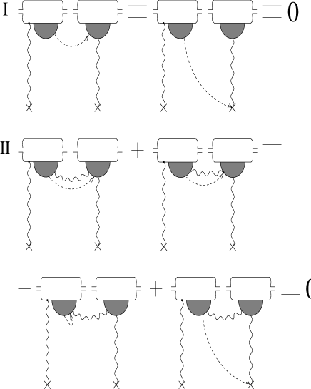
FIG. 8.: The way to eliminate many of the diagrams, which could appear in the nucleus-onium scattering.

For the graphs with two gluon fields the situation is a little more complicated. Here we have many more diagrams which disappear leaving only diagrams as in $C$ in Fig. 7. Most of the graphs with two gluon fields at order $g^{8}$, which are not equivalent to diagrams in class $C$, can be represented as having one gluon line, which gives the field, connected to some fermion line in nucleon number one, with the other three lines connected in all possible ways to provide one more gluon field, but not hooking to that first gluon line. Now, in each of these diagrams there must be one or two paths to get from one nucleon to the other along gluon lines. Each of these paths corresponds to some product of the propagator denominators. Due to the longitudinal separation between the nucleons , at least one of these denominators should include $1\over{l_{+}-i\epsilon}$. That is, it should correspond to a part of propagator which is longitudinally polarized at the right end, ${\eta_{\alpha}l_{\beta}\over{l_{+}-i\epsilon}}$, otherwise we would get either an exponential suppression as in (12) or a wrong ordering. Such a denominator should be present on each path from one nucleon to the other. This is illustrated in Fig. 8. The dashed line corresponds to the longitudinally polarized propagator, and is the same as in Fig. 4. The blobs represent some combinations of the gluon lines. Each graph is of order $g^{8}$. Case I corresponds to diagrams where there is only one path from one nucleon to the other along the gluon lines in the diagram. It also includes the case where there are two paths, but a longitudinally polarized line belongs to both of them. The situation where we have two paths between the nucleons and the longitudinally polarized lines are different for each of the paths is represented in case II. There we pick the longitudinally polarized line along one of the paths, without worrying much about the location of the similar line on the other path.

For case I in Fig. 8 we can just apply the Ward identity to get the diagram on the right, which is zero after color averaging in the right nucleon. By application of the Ward identity we mean summation over the contributions of the diagrams which have the same structure to the left and to the right of the dashed line, but different connections of the dashed line on the right hand side. The sum of these gives the graph on the right of I, similarly to Fig. 4. Analogously in case II in Fig. 8 we can apply the Ward identity to the dashed line. The result is shown in the second line of case II in Fig. 8. The first graph there corresponds to the arrow of the dashed line connected either to the vertex where the two paths split, if such vertex exists, or to the quark line in the first nucleon, if the paths do not overlap in the left blob. Now in both graphs there is only one path from one nucleon to another, and that brings us back to case I and cancels for the same reason. That way we include all the contributions from these diagrams and prove that they are zero.

FIG. 9.: Examples of the graphs that vanish (see text).

We illustrate our technique in Fig. 9. In general at order $g^{8}$ the graphs that we consider in Fig. 8 can be subdivided in two classes, representatives of which are shown in Fig. 9. We may have two gluons leaving nucleon number one to connect to nucleon number two [Fig. 9(a)]. There may also be just one such gluon [Fig. 9(b)]. The application of our method to the class of diagrams in Fig. 9(a) is straightforward. This obviously corresponds to case II in Fig. 8. At least one of the gluon lines connecting the nucleons should be longitudinally polarized. Summation over all of its possible connections on the right and application of the Ward identity leaves us with only one line connecting the nucleons. This line in its turn should be longitudinally polarized. Applying the Ward identity once again we get zero.

The diagrams represented in Fig. 9(b) are a little harder to deal with. The contribution in which line 1 is longitudinally polarized on the right belongs to case I in Fig. 8. Therefore, summing over all possible connections of line 1 on the right we get zero. When line 1 is covariant or longitudinally polarized at the left end we need either line 2 or line 3 to be longitudinally polarized at the right end. Let it be line 3. Now the situation corresponds to case II in Fig. 8. Applying the Ward identity we end up with the right end of line 3 hooking back to the three-gluon vertex or to the cross at the end of the gluon connected to the second nucleon. We took the contribution of line 1 which can not insure the longitudinal separation. Therefore, now line 2 has to be longitudinally polarized on the right. The situation again becomes similar to case I in Fig. 8. Summation over all possible connections of line 2 on the right gives us zero.

The diagrams which are not included in the representation shown in Fig. 8 can be eliminated by a similar technique. In the end we are left with the class of the diagrams $C$ in Fig. 7. The classical field at order $g^{5}$ is included in contributions of some of these diagrams. The initial and final states of the nucleons are color singlets. Therefore, color averaging in the first nucleon when calculating the graphs for the classical field at order $g^{5}$ in Sect. III is justified. There are no graphs with just one gluon field contributing to the scattering process, since we can not emit one gluon off a color singlet object.

So, the scattering process in light-cone gauge is described by the diagrams of the types shown in Fig. 7, i.e., by the classical field. If one thinks about this process in the covariant gauge, it is easy to see, that the only diagrams that contribute are of type $A$ in Fig. 7. It obviously is a combination of the classical fields. That way the correspondence can be easily seen in the covariant gauge. The two gluons per nucleon limit is also manifest in that gauge.

To conclude we summarize the results of this paper. The Feynman diagrams corresponding to the classical non-Abelian Weizsäcker-Williams field in the light-cone gauge were constructed (see Fig. 2, Fig. 3, Fig. 5 ). We derived a limit for the classical approach, which is two gluons per nucleon. It was shown that for a large nucleus the diagrams, satisfying this limit, which dominate a scattering process are described by a classical field (see Fig. 7). Therefore it is possible that the classical field may be used for calculation of such processes as charm production, dijet cross-section and many others in nuclear collisions.

REFERENCES

- [1] Yu. V. Kovchegov, Phys. Rev. D 54, 5463 (1996).
- [2] L. McLerran and R. Venugopalan, Phys. Rev. D 49, 2233 (1994); 49, 3352 (1994); 50, 2225 (1994).
- [3] A. Kovner, L. McLerran, and H. Weigert, Phys. Rev. D 52, 6231 (1995); 52, 3809 (1995).
- [4] J. Jalilian-Marian, A. Kovner, L. McLerran, and H. Weigert, hep-ph 9606337;J. Jalilian-Marian, hep-ph 9609350.
- [5] R. V. Gavai and R. Venugopalan, Phys. Rev. D 54, 5795 (1996).
- [6] G. t’Hooft, Nucl. Phys. B 33, 173 (1971).
- [7] G. Sterman, An Introduction to Quantum Field Theory , (Cambridge University Press, 1993).
- [8] S. J. Brodsky, G. P. Lepage, Phys. Rev. D 22, 2157 (1980).
- [9] A.H. Mueller, Nucl. Phys. B307, 34 (1988).