Abstract

A systematic study of large N expansion in supersymmetric theories are given. Supersymmetric O(N) non-linear sigma model in two and three dimensions, massless and massive supersymmetric QCD with $N_{f}<N_{c}-1$ and supergravity models are analyzed in detail. Our main motivation is to discuss how the previously studied mechanism for dynamical generation of gaugino condensation and superpotential is realized in the framework of large N expansion.

1 Introduction

When one extends the validity of the low energy effective field theory to energy scales much higher than its characteristic mass scale, one faces to a scale hierarchy problem. A typical example is the gauge hierarchy problem of the Standard Model of the strong and electroweak interactions, seen as a low-energy effective theory. When the Standard Model is extrapolated to cut-off scales $\Lambda\gg 1$Tev, there is no symmetry protecting the mass of the elementary Higgs field from acquiring large value, and therefore the masses of the weak gauge bosons, receive large quantum corrections proportional to $\Lambda$. The most popular solution to the gauge hierarchy problem of the Standard Model is to extend it to a model with global N=1 supersymmetry, effectively broken at a scale $M_{Soft}\sim 1$Tev. (See ref.[1] for a general review.) These extensions of the Standard Model, for instance the Minimal Supersymmetric Standard Model(MSSM), can be safely extrapolated up to cut-off scales much higher than the electroweak scale, such as the supersymmetric unification scale $M_{U}\sim 10^{16}$Gev, the string scale $M_{s}\sim 10^{17}$Gev, or Planck scale $M_{P}=2.4\times 10^{18}$Gev.

To go beyond the MSSM, one must move to a more fundamental theory with spontaneous supersymmetry breaking. The possible candidate for such a theory is N=1 supergravity coupled to gauge and matter fields, where the spontaneous breaking of local supersymmetry is not incompatible with vanishing vacuum energy[2]. (Of course, supersymmetry breaking can be transmitted by gauge interaction[3]. But here we concentrate on the supergravity mediated supersymmetry breaking models.) In N=1 supergravity, the spin 2 graviton has as superpartner, the spin 3/2 gravitino. Here we consider the case that the supersymmetry breaking is spontaneous, via the super-Higgs mechanism[4]. One is then bound to interpret the MSSM as an effective low-energy theory derived from spontaneously broken supergravity. The scale of soft supersymmetry breaking in MSSM, $M_{Soft}$, is related to the gravitino mass $m_{\frac{3}{2}}$, which sets the scale of the spontaneous breaking of local supersymmetry.

The idea of breaking supersymmetry in a dynamical way was first presented in ref.[6]. In those articles a general topological argument was developed in terms of the Witten index $Tr(-)^{F}$, showing that dynamical supersymmetry breaking cannot be achieved unless there is chiral matter or we include supergravity effects for which the index argument cannot apply. This is subsequently verified by explicitly studying gaugino condensation in pure supersymmetric Yang-Mills, a vector-like theory, for which gauginos condensate but do not break global supersymmetry. Breaking global supersymmetry with chiral matter was an open possibility in principle, but this approach ran into many problems when tried to be realized in practice[5].

The situation was improved very much with the coupling to supergravity. The reason was that the simple gaugino condensation was found to be sufficient to break supersymmetry once the coupling to gravity was included[7]. This works in the hidden sector mechanism where gravity is the messenger of supersymmetry breaking to the observable sector. However, this mechanism does not work when the gauge couplings are considered to be field dependent. Non-perturbative effects, like gaugino condensations, raises the moduli flat potentials, but it is very difficult to obtain a phenomenological vacuum state. The main difficulty lies in the runaway behavior of dilaton potential[8, 9]. Gaugino condensation with field dependent gauge couplings was anticipated and realized in a very natural way in string theory. The gauge couplings are functions of dilaton and moduli fields. Furthermore, string theory provides a natural realization of the hidden sector models by having a hidden sector[10]. Thus it is important to consider the following questions: Does gaugino really condensate in supergravity theories? If so, is runaway potential stabilized? If runaway potential is not stabilized by gaugino condensation, what effect should be responsible for the moduli fixing? We know that an ordinary effective Lagrangian analysis cannot give us a satisfactory answer and we think it is very important to develop new ideas to analyze the dynamical properties of supergravity theories. (Assuming the scenario of two or more gaugino condensates, the effective Lagrangian with confined hidden sector stabilizes the dilaton potential and breaks supersymmetry with a more complicated dilaton superpotential generated by multiple gaugino condensations[9]. However, one solution for the stabilization of the dilaton in the effective Lagrangian requires a delicate cancellation between the contributions from different gaugino condensates, which is not very natural. The other solution generally requires the assistance of an additional source of supersymmetry breaking[11, 12].) In this paper, we have developed a new method for the analysis of the dynamical properties of supersymmetry theories. Of course, as is recently discussed by many authors[13], we may find a solution to this problem by introducing a new type of non-perturbative effects. One of the very promising candidates is the effects of strongly coupled strings, but we do not consider this possibility because at this moment we are not sure how to handle and apply this idea to phenomenological models.

In this paper, we analyze several types of supersymmetric models by using large N expansion. In this limit, the relation between the effective Lagrangian approach with confined hidden sector and Nambu-Jona-Lasinio type approach is clarified. In large N limit, these two correspond to different kinds of approximations of the exact solution. Our main concern is to discuss how the previously mentioned mechanism for dynamical supergravity breaking is realized in the framework of the large N expansion. In Section 2, in order to discuss the applicability of large N expansion in supersymmetric theories, we consider a simple toy model. This model, O(N) sigma model, is very useful when one introduces large N expansion in supersymmetric theories. In Section 3, we use this method to analyze the dynamical properties of supersymmetric QCD. Finally in Section 4, we study the dynamical supersymmetry breaking in a local supersymmetric model. The driving force for gaugino condensation, which is not clear in other approaches, is now obvious. In general effective Lagrangian approach, the form of the potential for gaugino condensation is not well defined near the origin($\lambda\lambda\sim 0$) and it is difficult to understand how this condensation takes place. On the other hand, in Nambu-Jona-Lasinio type approach or in the large N expansion, the potential is given by the wine-bottle and we can easily imagine how fields rolls down to the condensating vacuum.

2 Supersymmetric O(N) non-linear sigma model

People generally tend to think that, in supersymmetric theories, no gap equations should exist because the non-renormalization theorem seems to ensure the cancellation of bosonic loops and fermionic ones. This is true for the superpotential motivated mass terms[14], but not applicable to the D-term motivated ones, such as a gaugino soft mass. Here, we should remember that N=1 four-dimensional non-renormalization theorem says nothing about the renormalization of D-terms but only about the superpotential renormalization [15].

We believe it is very important to show, first of all, that one can find a supersymmetric model in which we can exactly solve the gap-equation by means of large N expansion. Here we examine the phase structures of supersymmetric O(N) non-linear sigma model in two and three dimensions. We mainly follow refs.[16] and [17]. Some shortcomings of the previous papers on this topic are corrected and deeper insights are given.

2.1 Introduction

Many years ago, Gross and Neveu[18] have shown that dynamical symmetry breakdown is possible in asymptotically free field theories. They obtain an expansion in powers of $1/N$ that is non-perturbative in $g^{2}$. This leads to a massive fermion and to a $\overline{\psi}{\psi}$ bound state at threshold.

Polyakov[19] has pointed out that the $O(N)$ non-linear sigma model is asymptotically free and that the fundamental particle acquires a mass for $N>2$.

Witten [20] has constructed a supersymmetric version of the two-dimensional O(N) sigma model. This is a hybridization of the non-linear sigma model and Gross-Neveu model with Majorana fermions.

Then one question appears naturally. What is the difference between non-supersymmetric models and supersymmetric ones? If there is any difference, how is it realized? Many authors tried to answer this question[21, 22], but some questionable aspects of arguments are still left.

The purpose of this section is to clarify these ambiguities and present a systematic treatment of this model. To show explicitly what is going on, we are not going to eliminate the auxiliary fields at the first stage by using the equation of motion. If we eliminate all the auxiliary fields, it becomes difficult to find what relations we are dealing with.

2.2 Review of the non-linear sigma model

In this and the next subsections we are going to review the well-known results of O(N) non-linear sigma model and four-fermion model to fix the notations, and we show the strategy which is used throughout this paper.

The Lagrangian for O(N) sigma model is defined by

$$L=-\frac{1}{2}n_{j}\partial^{2}n_{j}$$ (2.1)

with the local non-linear constraint

$$n_{j}n_{j}=\frac{N}{g^{2}}.$$ (2.2)

The sum over the flavor index j runs from 1 to N. This constraint can be implemented by introducing a Lagrange multiplier $\lambda$.

Let us consider the Euclidean functional integral in the form:

$$Z = \int D\vec{n}\delta\left((\vec{n})^{2}-\frac{N}{g^{2}}\right)exp\left(-\frac{1}{2}\int(\partial_{\mu}\vec{n})^{2}d^{D}x\right)$$ (2.3)

$$= \int D\lambda\int D\vec{n}exp\left\{-\frac{1}{2}\int\left[(\partial_{\mu}\vec{n})^{2}+\lambda\left((\vec{n})^{2}-\frac{N}{g^{2}}\right)\right]d^{D}x\right\}$$

The integral over $n$ is Gaussian and can be performed in a standard fashion. We have:

$$Z=\int{D}\lambda{exp}\left(\frac{N}{2g^{2}}\int{\lambda}d^{D}x-\frac{N}{2}trln(-\partial^{2}+\lambda)\right)$$ (2.4)

Let us first compute the variation of the action with respect to $\lambda$. We get the following equation[23]:

$$\frac{N}{2g^{2}} = \frac{N}{2}\frac{\delta}{\delta\lambda(x)}trln(-\partial^{2}+\lambda(x))$$ (2.5)

$$= \frac{N}{2}G(x,x;\lambda)$$

Here we have introduced the Green function:

$$G(x,x^{\prime};\lambda)=<x^{\prime}|(-\partial^{2}+\lambda)^{-1}|x>$$ (2.6)

The meaning of the above equation becomes transparent if we notice that

$$<n_{i}(x)n_{j}(y)> = Z^{-1}\int{D}\lambda\int{D}\vec{n}exp\left(-\frac{1}{2}\int\left\{(\partial\vec{n})^{2}+\lambda\left(\vec{n}^{2}-\frac{N}{g^{2}}\right)\right\}d^{D}x\right)$$ (2.7)

$$\ \ \times{n}_{i}(x)n_{j}(y)$$

$$= \delta_{ij}\frac{\int{D}\lambda e^{-W}G(x,y;\lambda)}{\int{D}\lambda e^{-W}}$$

$$W = -\frac{N}{2g^{2}}\int\lambda{d}^{D}x+\frac{N}{2}trln(-\partial^{2}+\lambda).$$

If $\lambda$ integration is to be approximated by the saddle point $\lambda_{0}$, we obtain

$$<n_{i}(x)n_{j}(y)>=\delta_{ij}G(x,y;\lambda_{0}).$$ (2.8)

These equation shows that eq.(2.5) is nothing but the condition $<\vec{n}^{2}>=\frac{N}{g^{2}}$. In other words, the gap equation can be obtained directly from the constraint equation. Here we call this simple calculation a tadpole method after ref.[24]. Now let us solve eq.(2.5). Passing to the momentum representation, this “gap equation” is presented as:

$$G(x,x^{\prime};\lambda_{0}) = \int\frac{d^{D}p}{(2\pi)^{D}}\frac{e^{ip(x-x^{\prime})}}{p^{2}+\lambda_{0}}$$

$$\frac{N}{g^{2}} = NG(x,x;\lambda_{0})$$ (2.9)

$$= N\int\frac{d^{D}p}{(2\pi)^{D}}\frac{1}{p^{2}+\lambda_{0}}.$$

This equation is applicable for any $D$ dimensions. For D=2, we can obtain the precise form:

$$1 = \frac{g^{2}}{4\pi}log\frac{\Lambda^{2}}{\lambda_{0}}$$

$$\lambda_{0} = \Lambda^{2}exp\left(-\frac{4\pi}{g^{2}}\right)$$ (2.10)

For D=3, the situation differs slightly. We should include a critical coupling $g^{2}_{cr}$ defined by

$$1=g^{2}_{cr}\int\frac{d^{3}p}{(2\pi)^{3}}\frac{1}{p^{2}}.$$ (2.11)

If the coupling is strong($g^{2}>g^{2}_{cr}$), the gap equation has a non-trivial solution at $\lambda_{0}\neq 0$. (This critical coupling explicitly depends on the cut-off scale $\Lambda$, so in three dimensions, we regard this model as a low-energy effective theory of some high-energy physics. Of course one may find a good way to remove this cut-off dependence, but here we do not consider such a detailed analysis.) Using $g_{cr}$, we can rewrite (2.2) as:

$$1 = g^{2}\int\frac{d^{3}p}{(2\pi)^{3}p^{2}}-g^{2}\int\frac{d^{3}p}{(2\pi)^{3}}\left(\frac{1}{p^{2}}-\frac{1}{p^{2}+\lambda_{0}}\right)$$ (2.12)

$$= \frac{g^{2}}{g^{2}_{cr}}-g^{2}\int\frac{d^{3}p}{(2\pi)^{3}}\frac{\lambda_{0}}{p^{2}(p^{2}+\lambda_{0})}$$

The integral in (2.12) is convergent. Therefore, we have:

$$m^{2}\equiv\lambda_{0}=const.\left(\frac{1}{g^{2}_{cr}}-\frac{1}{g^{2}}\right)^{2}$$ (2.13)

If we take $g^{2}<g_{cr}^{2}$ something goes wrong with eq.(2.12). It does not have any solution, so the constraint $<\vec{n}^{2}>=\frac{N}{g^{2}}$ cannot be satisfied in this way. To solve this puzzle, we should also consider the possibility of spontaneous breaking of O(N) symmetry. In above discussions, we have implicitly assumed that the vacuum expectation value of $\vec{n}$ would vanish. Now we consider what will be changed if $\vec{n}$ itself gets a non-zero vacuum expectation value. Because of O(N) symmetry, the vacuum expectation value of $\vec{n}\equiv(n_{1},n_{2},...n_{N})$ may be written as

$$<\vec{n}>=(0,0,...\sqrt{N}v/g).$$ (2.14)

So that the constraint equation (2.2) is changed.

$$<(\vec{n})^{2}> = <\vec{n}>^{2}+<1-loop>$$ (2.15)

$$= N\left(\frac{v^{2}}{g^{2}}+\int\frac{d^{3}p}{(2\pi)^{3}}\frac{1}{p^{2}+\lambda_{0}}\right)=\frac{N}{g^{2}}$$

Of course, in two dimensions we cannot expect $\vec{n}$ to get any expectation value. Considering the spontaneous breaking of $O(N)$ symmetry, we introduce another important critical coupling constant $g^{\prime}_{cr}$.

$$\frac{1-v^{2}}{g_{cr}^{{}^{\prime}2}}=\int\frac{d^{3}p}{(2\pi)^{3}}\frac{1}{p^{2}}$$ (2.16)

If $g$ is smaller than $g_{cr}$, then $v$ grows such that the constraint equation is satisfied in the weak coupling region($g^{\prime}_{cr}\leq{g}\leq{g}_{cr}$) in a sense that not eq.(2.2) but eq.(2.15) is satisfied by some $\lambda_{0}$. There appears, however, a peculiar “flat direction” in three dimensions. As we have seen in the above analysis (2.15), the constraint equation is satisfied for arbitrary values of $\lambda_{0}$ and $v_{0}$ once a certain relation is satisfied by these two variables. To satisfy the constraint equation, $\lambda_{0}$ and $v$ should be related, but one cannot fix them at a unique point. This relation defines the “flat direction” of such a peculiar type. This is because once the constraint equation is satisfied, the potential term should vanish by definition.

As far as we deal with non-supersymmetric sigma model, we have no primary reason to believe that the vacuum expectation value of the field $v=<n_{j}>$ would vanish in the strong coupling region.

2.3 Review of the four-fermion model

The four-fermion model is described by the Lagrangian

$$L=\frac{i}{2}\overline{\psi}_{j}\not{\!\partial}\psi_{j}+\frac{g^{2}}{8N}(\overline{\psi}_{j}\psi_{j})^{2}$$ (2.17)

where the sum of the flavor index j runs from 1 to N and we require that $g^{2}$ remain constant as N goes to infinity. By introducing a scalar auxiliary field $\sigma$ ($\sigma=\frac{N}{2g^{2}}\overline{\psi_{j}}\psi_{j}$) we may rewrite (2.17) as

$$L=\frac{i}{2}\overline{\psi}_{j}\not{\!\partial}\psi_{j}+\frac{1}{2}\sigma\overline{\psi}_{j}\psi_{j}-\frac{N\sigma^{2}}{2g^{2}}.$$ (2.18)

Let us consider the functional integral in the form:

$$Z=\int{D}\psi_{j}D\sigma{exp}\left[\int{d}^{D}x\left\{\frac{1}{2}\overline{\psi}_{j}(i\not{\!\partial}+\sigma)\psi_{j}-\frac{N}{2g^{2}}\sigma^{2}\right\}\right]$$ (2.19)

Integrating over the field $\psi_{j}$ we get an effective action for the field $\sigma$:

$$Z=\int{D}\sigma{exp}\left[-\frac{N}{2g^{2}}\int{d}^{D}x\sigma^{2}+\frac{N}{2}Trln(i\not{\!\partial}+\sigma)\right]$$ (2.20)

We impose the stationary condition which gives the gap equation.

$$\frac{N<\sigma>}{g^{2}}-\frac{N}{2}\int\frac{d^{D}p}{(2\pi)^{D}}tr\frac{1}{-\not{\!p}+<\sigma>}=0$$ (2.21)

As is in non-linear sigma model discussed in the previous part of this section, this gap equation represents the condition

$$\frac{N}{g^{2}}<\sigma>=\frac{1}{2}<\overline{\psi}_{j}\psi_{j}>|_{m_{\psi}=<\sigma>}.$$ (2.22)

where non-zero $\sigma$ corresponds to the condensation of $\overline{\psi}_{j}\psi_{j}$. For D=2, we obtain the equation:

$$\frac{1}{g^{2}} = \int\frac{d^{2}p}{(2\pi)^{2}}\frac{1}{p^{2}+<\sigma>^{2}}$$

$$<\sigma>^{2} = \Lambda^{2}exp\left(-\frac{4\pi}{g^{2}}\right)$$ (2.23)

For D=3, we have a critical coupling constant. The saddle point exists only within the branch

$$0<\frac{1}{g^{2}}\leq\frac{1}{g_{cr}^{2}}$$ (2.24)

where

$$\frac{1}{g^{2}_{cr}}\equiv\int\frac{d^{3}p}{(2\pi)^{3}}\frac{1}{p^{2}}.$$ (2.25)

The crucial difference from the $O(N)$ non-linear sigma model is that eq.(2.22) always has a trivial solution at $\sigma=0$. In the weak coupling region, non-trivial saddle point vanishes but the trivial solution always exists.

2.4 Phases in Supersymmetric Non-Linear Sigma Model

Supersymmetric non-linear sigma model is usually defined by the Lagrangian

$$L=\frac{1}{2}\int{d}^{2}\theta(\overline{D}\Phi_{j})(D\Phi_{j})$$ (2.26)

with the non-linear constraint

$$\Phi_{j}\Phi_{j}=\frac{N}{g^{2}}.$$ (2.27)

where the sum of the flavor index j runs from 1 to N. The superfields $\Phi_{j}$ may be expanded in components

$$\Phi_{j}=n_{j}+\overline{\theta}\psi_{j}+\frac{1}{2}\overline{\theta}\theta{F}_{j}$$ (2.28)

and we define the super covariant derivative of the form:

$$D=\frac{\partial}{\partial\theta}-i\overline{\theta}\not{\!\partial}$$ (2.29)

In order to express the constraint (2.27) as a $\delta$ function, we introduce a Lagrange multiplier superfield $\Sigma$.

$$\Sigma=\sigma+\overline{\theta}\xi+\frac{1}{2}\overline{\theta}\theta\lambda$$ (2.30)

We thus arrive at the manifestly supersymmetric action for the supersymmetric sigma model.

$$S=\int{d}^{D}xd^{2}\theta\left[\frac{1}{2}(\overline{D}\Phi_{j})(D\Phi_{j})+\frac{1}{2}\Sigma\left(\Phi_{j}\Phi_{j}-\frac{N}{g^{2}}\right)\right]$$ (2.31)

where D=2,3. In component form, the Lagrangian from (2.31) is explicitly written in the following form.

$$L = -\frac{1}{2}n_{j}\partial^{2}n_{j}+\frac{i}{2}\overline{\psi}_{j}\not{\!\partial}\psi_{j}+\frac{1}{2}F_{j}^{2}-\sigma{n}_{j}F_{j}-\frac{1}{2}\lambda{n}_{j}^{2}$$ (2.32)

$$+\frac{1}{2}\sigma\overline{\psi}_{j}\psi_{j}+\overline{\xi}\psi_{j}n_{j}+\frac{N}{2g^{2}}\lambda$$

We can see that $\lambda,\xi,$ and $\sigma$ are the respective Lagrange multipliers for the constraints:

$$n_{j}n_{j} = \frac{N}{g^{2}}$$

$$n_{j}\psi_{j} = 0$$

$$n_{j}F_{j} = \frac{1}{2}\overline{\psi}_{j}\psi_{j}$$ (2.33)

The second and the third constraints are obtained by the supersymmetric transformations of the first one. We must not include kinetic terms for the field $\sigma$ and $\xi$ so as to keep these constraints manifest. We can examine these constraints in a manner we have used in the previous part of this section. As we have seen, we can directly solve the gap equation without calculating the explicit 1-loop potential. Below, we analyze each constraint and solve gap equations.

First we examine the two dimensional theory.

(1) Scalar part

$$<n_{j}n_{j}>|_{m_{n}^{2}=<\lambda>+<\sigma^{2}>}=\frac{N}{g^{2}}$$ (2.34)

In two dimensions, as we have seen above, $m_{n}$ is always non-zero.

$$m_{n}^{2} = <\lambda>+<\sigma>^{2}$$ (2.35)

$$= \Lambda^{2}exp\left(-\frac{4\pi}{g^{2}}\right)$$

This fixes $m_{n}$ at a dynamical scale but does not fix $<\lambda>$ and $<\sigma>^{2}$ independently.

(2) Fermion part

$$<n_{j}F_{j}>=\frac{1}{2}<\overline{\psi}_{j}{\psi}_{j}>$$ (2.36)

One may think that the fermionic condensation should vanish to keep supersymmetry unbroken, but this notion is not always true. This relation includes auxiliary field $F_{j}$, to be eliminated by equation of motion. After substituting $F_{j}$ by $\sigma{n}_{j}$, we obtain at one-loop level:

$$<n_{j}F_{j}> = <\sigma n_{j}n_{j}>$$ (2.37)

$$= <\sigma><n_{j}n_{j}>=\frac{1}{2}<\overline{\psi}_{j}\psi_{j}>$$

If we impose the O(N) symmetric constraint $<n^{2}>=\frac{N}{g^{2}}$, we have

$$\frac{N}{g^{2}}<\sigma> = \frac{1}{2}<\overline{\psi}\psi>|_{m_{\psi}=<\sigma>}$$

$$\frac{N}{g^{2}} = \frac{N}{2}\int\frac{dp^{D}}{(2\pi)^{D}}\frac{1}{p^{2}+<\sigma>^{2}}.$$ (2.38)

For D=2, the solution is

$$<\sigma>^{2}=\Lambda^{2}exp\left(-\frac{4\pi}{g^{2}}\right).$$ (2.39)

Substituting $<\sigma>$ in the first constraint (2.34) with (2.39), we can find that $<\lambda>$ must vanish(in this point ref.[22] was wrong). This means that the field $\psi$ gains the same mass as $n$, and simultaneously supersymmetric order parameter $<\lambda>$ vanishes. We can say that the supersymmetry is not broken in two dimensions as is predicted by Witten[6]. Moreover, we can examine the assumption of vanishing $v$ by decomposing the constraint(2.36) as follows.

$$<\sigma>\left(v^{2}+\int\frac{d^{2}p}{(2\pi)^{2}}\frac{1}{p^{2}+<\sigma>^{2}}\right)=\int\frac{d^{2}p}{(2\pi)^{2}}\frac{<\sigma>}{p^{2}+<\sigma>^{2}}$$ (2.40)

Bosonic and fermionic loops exactly cancel. Finally we obtain:

$$<\sigma>v^{2}=0$$ (2.41)

As $<\sigma>$ is non-zero in two dimensions(2.39), we must set $v=0$.

When D=3, we can find a solution for the eq.(2.34) only in the region $g>g^{\prime}_{cr}$. The critical coupling $g^{\prime}_{cr}$ is defined by

$$\frac{1-v^{2}}{g_{cr}^{{}^{\prime}2}}=\int\frac{d^{3}p}{(2\pi)^{3}}\frac{1}{p^{2}}$$ (2.42)

while $g_{cr}$ is defined as:

$$\frac{1}{g^{2}_{cr}}\equiv\int\frac{d^{3}p}{(2\pi)^{3}}\frac{1}{p^{2}}.$$ (2.43)

O(N) symmetry is expected to be spontaneously broken in the region $g^{\prime}_{cr}<g<g_{cr}$ by a non-zero value of $v$. And when $g=g^{\prime}_{cr}$, $m_{n}$ would vanish.

For the fermionic part(2.36), in D=3, we also have a critical coupling constant. As far as $g\geq{g}_{cr}$, we have nothing to worry about. In this strong coupling region, both supersymmetry and O(N) symmetry are preserved in a fashion like two dimensions. In this region $v$ cannot develop any non-zero value because eq.(2.41) is also true for the strongly coupled three dimensional theory. However, in the weak coupling region, something goes wrong. There is no non-trivial solution for fermionic constraint(2.36) and there is no fermionic condensation (This means that the only possible solution is $<\sigma>=0$). Thus we can see from eq.(2.41) that $v$ can develop non-zero value in this weak coupling region. This is supported by the constraint (2.34), because this does not have any solution in the weak coupling region unless we allow $v$ to develop non-vanishing value. Eq.(2.15) suggests:

$$v^{2}=1-g^{2}\int\frac{d^{3}p}{(2\pi)^{2}}\frac{1}{p^{2}}$$ (2.44)

Naive consideration also supports this analysis. In general, we can expect that quantum effects in correlation functions like $<n_{j}n_{j}>$ or $<\overline{\psi}\psi>$ would vanish in the weak coupling limit. But we have a O(N) symmetric constraint. It is natural to think that the field $n$ itself gains expectation value to complement quantum effects. This simply means that classical effects become more dominant in the weak coupling region, therefore the O(N) symmetric constraint is satisfied classically. (i.e. in the weak coupling limit $g\rightarrow 0$ we obtain $v=1$. This is a classical solution of the constraint.) As a result, in the weak coupling region O(N) symmetry is spontaneously broken by non-zero value of $v$.

We should also note that, in the weak coupling region, there is also a possible solution of non-zero $\lambda_{0}$ if $g\neq g^{\prime}_{cr}$. It induces a supersymmetry breaking term to the Lagrangian of the form:

$$L_{break}=\lambda_{0}\left((\vec{n})^{2}-\frac{N}{g^{2}}\right)$$ (2.45)

On the constrained phase space($(\vec{n})^{2}-\frac{N}{g^{2}}=0$), vacuum energy also seems to vanish for non-zero $\lambda_{0}$ as far as $v$ valances to satisfy the constraints. (See section 2.2.) Can we think that there remains some unusual type of flat direction, with non-zero value of F-component? Of course this statement is wrong. After including effective kinetic terms, $\sim\lambda\lambda$ appears effectively(see ref.[25]). Then, we can find positive vacuum energy for supersymmetry breaking phase($\lambda\neq 0$) as in the usual type of supersymmetric theories. So we can conclude:

(1) In two dimensions, both supersymmetry and O(N) symmetry are not broken. This means that $\lambda$ and $v$ remain zero for any value of $g$.

(2) In three dimensions, both supersymmetry and O(N) symmetry are not broken (i.e. $\lambda$ and $v$ remain zero) in the strong coupling region. O(N) symmetry can be broken in the weak coupling region, but supersymmetry is kept unbroken in both phases.

2.5 Some peculiar properties of the present model

In this section we discuss the stability of the dynamically generated supersymmetric mass terms against the supersymmetry breaking mass term.

We examine the supersymmetric non-linear O(N) sigma model with a supersymmetry breaking mass term. In two dimensions, we will find that the mass difference between supersymmetric partner fields vanishes by the quantum effect. In three dimensions, the mass difference vanishes in the strong coupling region, but O(N) symmetry is always broken both in strong and weak coupling region.

To see what happens, now let us extend the above analysis to include a supersymmetry breaking mass term. Here we consider a supersymmetry breaking mass term of the form:

$$L_{break}=\frac{-1}{2}m_{s}^{2}n_{j}^{2}$$ (2.46)

Including this supersymmetry breaking mass term, we can calculate the gap equation explicitly. For the scalar part it becomes:

$$n_{j}n_{j}|_{m_{n}^{2}=<\lambda>+<\sigma>^{2}+m_{s}^{2}} = N\int\frac{d^{D}p}{(2\pi)^{D}}\frac{1}{p^{2}+<\lambda>+<\sigma>^{2}+m_{s}^{2}}$$ (2.47)

$$= \frac{N}{g^{2}}$$

The fermionic part is unchanged by the supersymmetry breaking mass term. For $D=2$ we can solve this equation explicitly.

$$1 = \frac{g^{2}}{4\pi}log\frac{\Lambda^{2}}{<\lambda>+<\sigma>^{2}+m_{s}^{2}}$$

$$m_{n}^{2} = <\lambda>+<\sigma>^{2}+m_{s}^{2}$$ (2.48)

$$= \Lambda^{2}exp\left(-\frac{4\pi}{g^{2}}\right)$$

$<\sigma>^{2}$ is determined by the fermionic part which is unchanged by the supersymmetry breaking term(2.46).

$$m_{\psi}^{2} = <\sigma>^{2}$$ (2.49)

$$= \Lambda^{2}exp\left(-\frac{4\pi}{g^{2}}\right).$$

These two equations suggest two consequences. One is that the order parameter for supersymmetry breaking($\lambda$) gets non-zero value. The shift of $\lambda$ that is induced by the supersymmetry breaking mass term is:

$$<\lambda>+m^{2}_{s}=0$$ (2.50)

And supersymmetry is broken. The second consequence is more peculiar. As we can see from explicit calculations, dynamically generated masses are unchanged and the mass degeneracy is not removed by the explicit supersymmetry breaking mass term. This happens because the auxiliary field $\lambda$ has absorbed $m_{s}$ so that the two masses balance.

We conclude that, if we believe the validity of the large N expansion, the dynamical masses are unchanged while the supersymmetry breaking parameter develops non-zero value.

The crucial point of our observation lies in the fact that we can absorb the supersymmetry breaking mass term by redefining a field. The simplest and trivial example is the ordinary O(N) non-linear sigma model with an explicit mass term. This is written as:

$$L=-\frac{1}{2}n_{j}\partial^{2}n_{j}-\frac{1}{2}\lambda(n_{j}^{2}-\frac{N}{g^{2}})-m^{2}_{s}n_{j}^{2}$$ (2.51)

Does the explicit mass term changes the dynamical mass? The answer is no. This can easily be verified by redefining $\lambda$ as $\lambda^{\prime}=\lambda+m^{2}_{s}$. Lagrangian is now:

$$L=-\frac{1}{2}n_{j}\partial^{2}n_{j}-\frac{1}{2}\lambda^{\prime}(n_{j}^{2}-\frac{N}{g^{2}})-\frac{N}{2g^{2}}m^{2}_{s}$$ (2.52)

We can find that the mass term is absorbed in $\lambda^{\prime}$ and only a constant is left. Of course, this constant does not change the gap equation.

In three dimensions, however, it is not so simple. Many fields and their equations form complex relations and determine their values each other. Let us see more details. In three dimensions, things are not so easy. As is discussed above, this model has a weak coupling region where no dynamical mass is produced so no balancing effect between superpartner masses works in this region. Setting $\lambda=0$, we find $m_{n}=m_{s}$ and $m_{\psi}=0$ when $g$ is small. This agrees with the naive expectation. What will happen if we go into the strong coupling region where the gap equations develop non-trivial solutions and the fermion becomes massive? If there were no supersymmetry breaking mass term, O(N) symmetry restoration occurs in this region. But because $m_{s}$ is non-zero, $v$ must develop non-zero value in order to compensate $m_{s}$ and satisfy the constraint equation(2.15). In this case, we cannot set $\lambda=0$ because $\lambda$ and $v$ should be determined by minimizing the full 1-loop potential.

To summarize, after adding a breaking term, some fields slide to compensate $m_{s}$ but the mechanism is not trivial. Even in our simplest model, many complex relations determine their values. In two dimensions, we found that the mass difference between supersymmetric partner fields vanishes but the supersymmetry is still broken in a sense that $<\lambda>$ is non-zero. In three dimensions, the mass difference is always non-zero. In the weak coupling region it is $m_{s}$, but to determine the precise value of the mass difference in the strong coupling region, we should solve the following equation:

$$n_{j}n_{j}|_{m_{n}^{2}=<\lambda>+<\sigma>^{2}+m_{s}^{2}} = v^{2}+N\int\frac{d^{3}p}{(2\pi)^{3}}\frac{1}{p^{2}+<\lambda>+<\sigma>^{2}+m_{s}^{2}}$$ (2.53)

$$= \frac{N}{g^{2}}$$

where $\sigma$ should be determined by the fermionic constraint. This equation (2.53) determines the relation between $v$ and $\lambda$. To go further, we should minimize the full 1-loop potential for $v$ and $\lambda$ under the constraint(2.53). This calculation is too complicated to find exact solutions, but it is obvious that $v$ and $\lambda$ are simultaneously non-zero. So we can conclude that in the strong coupling region, mass difference is non-zero and O(N) symmetry is also broken. In three dimensions O(N) symmetry is always broken and mass difference is always non-zero. Its value (mass difference) coincides with $m_{s}$ in the weak coupling region, but in the strong coupling region it is determined by very complicated relations.

What is new in this section is:

1) It was previously believed that the fermionic condensation is parameterized by $\lambda$ which is the F-component of the Lagrange multiplier. In ref.[22], it is discussed that even if fermionic condensation occurs and $\lambda$ becomes non-zero, supersymmetry is still maintained since the dynamical masses for fermion and scalar field are equal. By using tadpole method, we showed that $\lambda$ should vanish in this theory.

2) If one calculates a naive 1-loop effective potential, one will find a fictitious negative energy solution at $\lambda\neq 0$. This problem can be evaded if effective $\lambda\lambda$ term is included.

3) We analyzed the effects of the supersymmetry breaking mass term on dynamical properties.

Recently, many groups have discussed the dynamical properties of softly broken supersymmetric theories[26], but some non-trivial assumptions were needed. (For example, they assumed that the non-perturbative superpotential $W^{np}$ is not changed by the small soft mass. This is a very strong assumption which should be verified in another way. To be more specific, in O(N) non-linear sigma model this assumption corresponds to: Neglect the $m_{s}$ factor in the gap equations (2.5) and (2.53). Of course, this is obviously wrong.) Although our model is much simpler, we think it is important to consider the explicitly solvable models as a toy model for these complicated issues.

2.6 Summary of section 2

In this section we have studied supersymmetric O(N) non-linear sigma model in two and three dimensions. Supersymmetric O(N) non-linear sigma model is already analyzed in refs.[22, 25] by using 1-loop effective potential, but some uncertainties were left. (See 1),2) and 3) in the last part of the previous subsection.) Using tadpole method, we have re-analyzed this theory and found that this method is very useful especially when we analyze large N expansions in supersymmetric theories. Many uncertainties are resolved. We have also considered the effect of the supersymmetry breaking mass term and its peculiar properties.

3 Dynamical analysis in supersymmetric gauge theories

3.1 General Analysis

3.1.1 Supersymmetric pure Yang-Mills theory

Let us first review the dynamical analysis of supersymmetric Yang-Mills theory. In this paper, the word pure supersymmetric Yang-Mills theory(SYM) means the supersymmetric gauge theory with $SU(N_{c})$ gauge group without matter field.

The Lagrangian is generally written as:

$$L=\frac{1}{g^{2}}\int d^{2}\theta W^{\alpha a}W^{\alpha}_{a}+h.c.$$ (3.1)

where the chiral representation of the vector superfield ($W^{\alpha}$) contains gauge boson($A_{\mu}$) and its fermionic partner($\lambda^{\alpha}$).

$$W_{\alpha}^{a} = -i\lambda_{\alpha}^{a}+\left[\delta_{\alpha}^{\beta}D^{a}-\frac{i}{2}(\sigma^{\mu}\overline{\sigma}^{\nu})_{\alpha}^{\beta}(\partial_{\mu}A^{a}_{\nu}-\partial_{\nu}A^{a}_{\mu}+f^{abc}A^{b}_{\mu}A^{c}_{\nu})\right]\theta_{\beta}$$ (3.2)

$$+\theta\theta(\sigma^{\mu})_{\alpha\dot{\alpha}}\partial_{\mu}\overline{\lambda}^{a\dot{\alpha}}$$

It is known that Witten index is non-zero in this theory, so we can expect that supersymmetry should not be broken. On the other hand, it is also known that gaugino should condensate and chiral symmetry is broken. This condensation can be checked by the instanton calculation in the weak coupling region or by using the effective (confined) Lagrangian analysis in the strong coupling region. These analyses present consistent results so we can believe that gaugino condensation occurs in supersymmetric pure Yang-Mills theory at any scale.

For later convenience, here we explicitly calculate the effective potential for the composite field $U=\frac{g^{2}}{32\pi^{2}}W^{\alpha}W_{\alpha}$. Other approaches, such as the instanton calculation, are entirely reviewed in ref.[5]. The underlying principle of this construction is t’Hooft’s anomaly matching condition, which demands that the effective low energy Lagrangian, valid below some scale $\Lambda$, should reproduce the anomalies of the underlying constituent theory. In the case of the pure supersymmetric Yang-Mills model it is well known that R-symmetry and supersymmetry current as well as the energy momentum tensor lie in the same supersymmetry multiplet.

In terms of constituent fields the lowest component of $U$ is proportional to the gaugino bilinear $\lambda\lambda$, so it makes sense to take $U$ as the goldstone multiplet entering the low energy Lagrangian. The R-symmetry acts as

$$U(x,\theta)\rightarrow e^{3i\alpha}U(x,e^{-3i\alpha}\theta)$$ (3.3)

while the scale symmetry acts as

$$U(x,\theta)\rightarrow e^{3\gamma}U(xe^{\gamma},\theta e^{\gamma/2})$$ (3.4)

Assuming that the anomalies associated with the above classical invariances are reproduced by the superpotential $W$, one obtains the holomorphic equation for the superpotential (note that the imaginary part of $U$ contains $\tilde{F}F$)

• Anomaly from fundamental Lagrangian

  $$\delta L = 2N_{c}\alpha\frac{g^{2}}{32\pi^{2}}F\tilde{F}$$ (3.5)

  $$= 2N_{c}\alpha i\int d^{2}\theta U+h.c.$$

• Anomaly from composite Lagrangian

  $$\int d^{2}\theta(-2i\alpha W+2i\alpha U\frac{dW}{dU})+h.c.$$ (3.6)

The resulting anomaly matching condition is:

$$U\frac{\partial W}{\partial U}-W=N_{c}U,$$ (3.7)

which has the general solution of the form

$$W=aU+N_{c}Ulog\left(\frac{U}{\mu^{3}}\right)$$ (3.8)

where $a$ is in general undetermined and corresponds to the rescaling of the condensation scale $\mu$, and b is a function of the gauge coupling which is fixed by the anomaly constraints.

To examine this model explicitly, we need some information on the Kähler potential $K$. Usually one demands that the variation of the D-component of K is non-anomalous and it fixes its form to be:

$$K=const.(U\overline{U})^{1/3}$$ (3.9)

(If one takes $K=K(U\overline{U})$ then the variation vanishes identically for R-symmetry. However the variation under scale symmetry suggests that

$$\delta K|_{D}=\gamma\left[3\frac{\partial K}{\partial U}U+3\frac{\partial K}{\partial\overline{U}}\overline{U}-2K\right]_{D}$$ (3.10)

where only $K=const.(U\overline{U})^{1/3}$ is allowed.)

This leads to the effective potential of the form:

$$V=(K_{U\overline{U}})^{-1}|U|^{2}\left|(a+N_{c})+N_{c}log(\frac{U}{\mu^{3}})\right|^{2}$$ (3.11)

This scalar potential has the minimum at $U=\mu^{3}e^{-(a+N_{c})/N_{c}}e^{2\pi i/N_{c}}$ which agrees with the analysis of the instanton calculations. This also agrees with the Witten index analysis, which suggests that this theory has supersymmetric vacuum with non-zero gaugino condensation. One may find an extra minimum at the origin($U=0$), but because it corresponds to a vanishing point of $K_{U\overline{U}}$ and it also contradicts to other approaches(Witten Index and the instanton calculation) we may think that the effective potential is not well defined near the origin and discard this possibility of finding a trivial minimum at $U=0$. (See Fig.(1).)

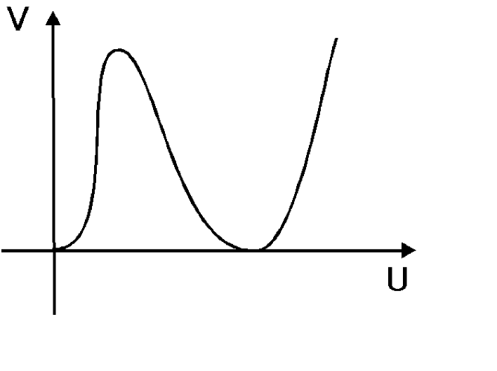
Figure 1: The scalar potential for gaugino condensate(U) for general supersymmetric Yang-Mills theory.

Here we also consider an important extension of the model, that is, inclusion of field dependent coupling constant. This extension is well motivated by the superstring effective Lagrangian or other effective Lagrangian analysis. Assuming that the inverse of the gauge coupling constant is given by a function $f(S)$, where $S$ denotes a gauge singlet superfield, we obtain an effective Lagrangian of the form:

$$L=\int d^{4}\theta[K(S,\overline{S})+K(U,\overline{U})]+\int d^{2}\theta[f(S)U+bUlog(\frac{U}{\mu^{3}})]+h.c.$$ (3.12)

The implication of the field dependent coupling constant is mainly discussed by the additional term in the scalar potential, which generally implies supersymmetry breaking (or runaway behavior) that is induced by gaugino condensation. The explicit form of the scalar potential is:

$$V=K_{U\overline{U}}^{-1}|f+b+blog(\frac{U}{\mu^{3}})|^{2}+K^{-1}_{S\overline{S}}|U|^{2}|\frac{\partial f}{\partial S}|^{2}$$ (3.13)

The second term originates from the present gauge singlet superfield and breaks supersymmetry when gaugino condenses. If gaugino condensation vanishes at $S\rightarrow\infty$, this implies a runaway behavior of this potential. We show the explicit form of this potential in Fig.(2).

For later convenience, let us examine the most popular example, $f(S)=S$ and $K(U,\overline{U})=(U\overline{U})^{1/3}$. In this case we obtain two solutions. One is $U=0$ and $S$ arbitrary, and the other is $U\rightarrow 0$ and $S\rightarrow\infty$.

Figure 2: Eq.(3.13)is plotted. It is easy to find that gaugino condensation breaks supersymmetry once the gauge coupling constant becomes field dependent.

3.1.2 Supersymmetric QCD

According to Witten index theorem, supersymmetry should not be broken in many theories. In particular, he has computed the index in pure SU(N) Yang-Mills theory and shown that this theory always has at least N supersymmetric ground state. This suggests that supersymmetry is not broken also in supersymmetric QCD theories with any number of massive fields.

However, the index theorem says nothing about the theory with massless quarks. This theory has (classical) flat directions along which fields can develop any value.

In this subsection we review the analysis on the dynamical effects in massless and massive supersymmetric QCD and show that in supersymmetric QCD with the number of flavors $N_{f}$, less than $N_{c}$, a dynamical superpotential is in fact generated. This potential is given for the composite(confined) fields for $N_{f}\leq N_{c}-1$. (In this case dynamical superpotential is generated by a strong coupling effect and there remains uncertainty in this calculation at small field strength. This uncertainty can be evaded by a peculiar assumption, that the low-energy theory, which can be thought as a pure Yang-Mills theory coupled to an R-Axion, has the same characteristics as the pure Yang-Mills theory. If this assumption is correct, we can expect that gaugino condensation is always non-zero even in the weak coupling limit.) For $N_{f}=N_{c}-1$, the instanton number constraint does not forbid the generation of the dynamical superpotential and we can show its generation by an explicit computation. However for $N_{f}<N_{c}-1$, because of the constraint from the instanton number, we should think that instanton is not responsible for the generation of dynamical superpotential. (The F-term carries charge 2 under $U(1)_{R^{\prime}}$ which cancels the charge -2 from the grassmannian integral. On the other hand, from

$$\partial_{\mu}j^{\mu}_{R}=\frac{1}{32\pi^{2}}2(N_{f}-N_{c})F^{a}\tilde{F}^{a}$$ (3.14)

we learn that instanton carries charge $2|N_{c}-N_{f}|$ under $U(1)_{R}$ symmetry. Thus we can see that the instanton-induced dynamical potential is allowed only for $N_{f}=N_{c}-1$.) Because we usually think that the instanton effects will dominate the dynamical effects in the weak coupling region, we think that the uncertainty does not exist for $N_{f}=N_{c}-1$. On the other hand, when $N_{f}<N_{c}-1$, we should consider another dynamical effect.

To obtain dynamical understanding of these theories, many authors attempted to construct effective Lagrangians to describe the low-energy dynamics of these theories. These analysis made it clear that in these theories with massive quarks, the limit $m_{q}\rightarrow 0$ was likely to be peculiar. In particular, it was shown that if a dynamical superpotential is generated in supersymmetric QCD with massless quarks by non-perturbative effects, its form is uniquely determined by the symmetric constraints. Moreover, if a small mass term is added to this theory, we can obtain N vacuum states which agrees with the index arguments. (Of course tree level superpotential can alter the symmetries of the theory, which have constrained the dynamical superpotential in massless theories. Above we assumed that a small mass term will not change the qualitative character of the dynamical potentials.)

Let us see more concrete examples. Here we mainly follow the paper ref.[27] which we regard as a “general” analysis.

By supersymmetric QCD we will mean a supersymmetric theory with gauge group $SU(N_{c})$ and $N_{f}$ flavors of quarks. The $N_{f}$ quark flavors correspond to $N_{f}$ chiral fields in the $N_{c}$ representation and $N_{f}$ chiral fields in the $\overline{N}_{c}$ representation.

$$Q^{ir}(i=1,...,N_{c};r=1,...,N_{f}), \overline{Q}_{ir}(i=1,...,N_{c};r=1,...,N_{f})$$ (3.15)

These superfields can be written with component fields as:

$$\left\{\begin{array}[]{l}Q^{ir}=\phi^{ir}+\theta^{\alpha}\psi_{\alpha}^{ir}+\theta^{2}F^{ir}\\ \overline{Q}_{ir}=\overline{\phi}_{ir}+\theta_{\alpha}\overline{\psi}^{\alpha}_{ir}+\theta^{2}\overline{F}_{ir}\end{array}\right.$$ (3.16)

The gauge fields $A^{a}_{\mu}(a=1,...,N_{c}^{2}-1)$ are included in vector multiplets $V^{a}$ accompanied by their super-partners, gauginos $\lambda^{a}$ and auxiliary fields $D^{a}$. The total theory is given by

$$L = \frac{1}{4g^{2}}\int d^{2}\theta W^{\alpha a}W_{\alpha}^{a}+h.c.+\int d^{4}\theta\left[Q^{+}e^{V}Q+\overline{Q}e^{-V}\overline{Q}^{+}\right]$$ (3.17)

Classically, this theory has a global $U(N_{f})_{Left}\times U(N_{f})_{Right}\times U(1)_{R}$ symmetry. The $U(N_{f})_{Left}\times U(N_{f})_{Right}$ symmetry is just like that of the ordinary QCD, corresponding to separate rotation of the $Q$ and $\overline{Q}$ fields. The symmetry $U(1)_{R}$ is an R-invariance, a symmetry under which the components of a given superfield transform differently. This corresponds to a rotation of the phases of the grassmannian variables $\theta^{\alpha}$,

$$\left\{\begin{array}[]{lll}\lambda&\rightarrow&e^{i\alpha}\lambda\\ \psi&\rightarrow&e^{i\alpha}\psi\\ \overline{\psi}&\rightarrow&e^{i\alpha}\overline{\psi}\end{array}\right.$$ (3.18)

with scalar and vector fields unrotated. This can be written as:

$$\left\{\begin{array}[]{lll}W_{\alpha}(\theta)&\rightarrow&e^{-i\alpha}W_{\alpha}(\theta e^{i\alpha})\\ Q(\theta)&\rightarrow&Q(\theta e^{i\alpha})\\ \overline{Q}(\theta)&\rightarrow&\overline{Q}(\theta e^{i\alpha}).\end{array}\right.$$ (3.19)

Just as in the ordinary QCD, some of these symmetries are explicitly broken by anomalies. A simple computation shows that the following symmetry, which is a combination of the ordinary chiral $U(1)_{A}$ and the $U(1)_{R}$ symmetry, is anomaly-free.

$$\left\{\begin{array}[]{lll}W_{\alpha}(\theta)&\rightarrow&e^{-i\alpha}W_{\alpha}(\theta e^{i\alpha})\\ Q(\theta)&\rightarrow&e^{i\alpha(N_{c}-N_{f})/N_{f}}Q(\theta e^{i\alpha})\\ \overline{Q}(\theta)&\rightarrow&e^{i\alpha(N_{c}-N_{f})/N_{f}}\overline{Q}(\theta e^{i\alpha})\end{array}\right.$$ (3.20)

From now on, we call this non-anomalous global symmetry $U(1)_{R^{\prime}}$.

It is important to stress that we are not looking for an explicit breaking of supersymmetry. Since it is believed that the supersymmetry current has no anomalies, the effective lagrangian should be supersymmetric and should be given by superfields. Its vacua, of course, need not to respect supersymmetry and other symmetries. The effective Lagrangian must respect all the (non-anomalous) symmetries whether the various symmetries of the theory is broken or not. Thus the dynamical superpotential which may be generated must be gauge and $G=SU(N_{f})_{Left}\times SU(N_{f})_{Right}\times U(1)_{V}\times U(1)_{R^{\prime}}$ invariant. To be gauge and $SU(N_{f})_{Left}\times SU(N_{f})_{Right}\times U(1)_{V}$ invariant, such a F-term must be of the form:

$$F\sim\int d^{2}\theta f(det_{rr^{\prime}}\overline{Q}_{ir}Q^{ir^{\prime}})$$ (3.21)

Further requirement from R’-invariance determines the precise form as:

$$F\sim\int d^{2}\theta(det_{rr^{\prime}}\overline{Q}_{ir}Q^{ir^{\prime}})^{-1/(N_{c}-N_{f})}$$ (3.22)

This term is only meaningful for $N_{f}<N_{c}$. For $N_{c}=N_{f}$, it is meaningless. For $N_{f}>N_{c}$, it vanishes identically by a simple symmetry argument. The coefficient of this F-term should be dimensionful, and must be given by a power of the dynamically generated scale of the theory($\Lambda$), which can be related to the scale of gaugino condensation.

$$F=const.\Lambda^{\frac{3N_{c}-N_{f}}{N_{c}-N_{f}}}\int d^{2}\theta(det_{rr^{\prime}}\overline{Q}_{ir}Q^{ir^{\prime}})^{\frac{-1}{N_{c}-N_{f}}}$$ (3.23)

The question of whether the dynamics indeed generates this term or not is of course another problem and will be discussed in the following. (See also ref.[27].)

In $N_{f}=N_{c}-1$, we can show that this term can be constructed by an explicit instanton calculation, so the dynamical origin is clear in this case.

Since this model has flat directions, it is reasonable to expect that $Q$ and $\overline{Q}$ may develop their vacuum expectation values along these directions. When $N_{f}<N-1$, because instanton does not allow the generation of (3.23), we should explain its generation from another point of view. In this case, the gauge group is not completely broken and we can expect that the intermediate scale Lagrangian, which appears after gauge symmetry breaking, is pure Yang-Mills theory coupled to an axion superfield. At energies below the symmetry breaking scale, assuming that the supersymmetry is not explicitly broken by perturbative effects, we can obtain an effective Lagrangian:

$$L = \int d^{2}\theta\frac{1}{4g^{2}}\left[1+\beta ln\left(\frac{\phi}{\Lambda}\right)\right]W^{\alpha}W_{\alpha}+h.c.$$

$$\beta = \frac{g^{2}}{32\pi^{2}}N_{f}$$ (3.24)

where $\beta$ is determined by R-anomaly. Eq.(3.1.2) contains a dimension five operator:

$$L_{AUX}=\frac{\beta g^{2}\lambda\lambda}{v}F_{\phi}+h.c.+F^{*}_{\phi}F_{\phi}$$ (3.25)

where $v$ is the symmetry breaking scale of $SU(N_{c})\rightarrow SU(N_{c}-N_{f})$, which can be identified with the cut-off scale of this effective Lagrangian. The field $\phi$ is considered as an anomaly compensating field for the non-anomalous R’ symmetry of the original Lagrangian. When $N_{c}=3$ and $N_{f}=1$, this effective Lagrangian is explicitly calculated by integrating the heavy fields[28]. This extra term in $L_{AUX}$ is very important when we think about the dynamical breaking of supersymmetry. Using the equation of motion for $F_{\phi}$, we obtain the relation

$$<F^{*}_{\phi}>\sim<\lambda\lambda>/v$$ (3.26)

this means that once gaugino condensates in the effective Yang-Mills theory, supersymmetry should be broken dynamically. At the same time, the flat direction along $\phi$ is lifted, but the shape of this potential is rather problematic. Its minimum lies at infinity, so this potential is called “Run-away” potential.(See also Fig.(3).) Of course we can use eq.(3.13) to obtain dynamical superpotential.

We should not forget that when $\phi$ rolls down to infinitely large value and run into the weakly coupled region, there remains uncertainty for $N_{f}<N_{c}-1$.

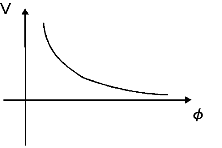
Figure 3: The flat direction is lifted but there remains a problematic behavior. This potential presents the so-called “Runaway potential”.

So far we have dealt with supersymmetric QCD with massless matters and we have discussed the generation of non-trivial superpotential for $N_{f}<N_{c}-1$. Here we analyze the same theory with (small) mass term for matter fields. The supersymmetric mass term is written as:

$$\int d^{2}\theta\sum^{N_{f}}_{k=1}m_{k}\overline{Q}_{ik}Q^{ik}$$ (3.27)

For simplicity, we assume that all the masses are equal. This mass term raises all the flat directions. According to Witten[6], this theory has al least $N_{c}$ supersymmetric vacua and supersymmetry is not broken by any dynamical effects. To show how this vacua are realized in the dynamical phase, we would like to discuss the symmetries of the massive QCD.

If this theory does not contain any mass term, the symmetry is(see the previous section):

$$G=SU(N_{f})_{Left}\times SU(N_{f})_{Right}\times U(1)_{V}\times U(1)_{R}$$ (3.28)

This symmetry is broken by the mass term. The continuous part of the remaining symmetry is:

$$SU(N_{f})\times U(1)_{V}$$ (3.29)

where $SU(N_{f})$ is the vector subgroup of $SU(N_{f})_{Left}\times SU(N_{f})_{Right}$. Besides this continuous symmetry, this theory has discrete $Z_{2N_{c}}$ symmetry:

$$W(\theta) \rightarrow e^{-i\pi n/N_{c}}W(\theta e^{i\pi n/N_{c}})$$

$$Q(\theta) \rightarrow e^{-i\pi n/N_{c}}Q(\theta e^{i\pi n/N_{c}})$$

$$\overline{Q}(\theta) \rightarrow e^{-i\pi n/N_{c}}\overline{Q}(\theta e^{i\pi n/N_{c}})$$

$$n = 1,...,2N_{c}$$ (3.30)

Witten has suggested that the $N_{c}$ vacua counted by index argument might be associated with the spontaneous breaking of this symmetry to a $Z_{2}$ subgroup. As far as the quark mass is small and can be considered as a small perturbation, one can show that the dynamical superpotential is still generated. The full superpotential is given by:

$$W_{dyn}=const.\Lambda^{\frac{3N_{c}-N_{f}}{N_{c}-N_{f}}}(det\overline{Q}Q))^{\frac{-1}{N_{c}-N_{f}}}+m\overline{Q}Q$$ (3.31)

This superpotential has N supersymmetric vacua of the form:

$$<\overline{Q}Q> = \Lambda^{3-\frac{N_{f}}{N_{c}}}\left(\frac{const.}{m(N_{c}-N_{f})}\right)^{-1+\frac{N_{f}}{N_{c}}}e^{2\pi in/N_{c}}$$

$$n = 1,...,N_{c}$$ (3.32)

This means that supersymmetric equation has exactly $N_{c}$ different solution. The runaway potential is thus stabilized and supersymmetric vacuum is now well defined. (See Fig.(4)

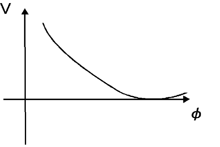
Figure 4: The scalar potential for SQCD with small mass term. The asymptotic behavior is changed. No runaway is observed and supersymmetry is kept unbroken.

3.2 Large N expansion of global supersymmetric models

In this section, we will discuss dynamical properties of global supersymmetric gauge theories in terms of large N expansion. This method can easily be extended to supergravity models [29, 30].

3.2.1 Gaugino condensation in supersymmetric QCD

Gaugino condensation in supersymmetric gauge theories has been extensively studied by many authors both in global[5] and local[31] theories. In this section we examine the vacuum structures of Supersymmetric QCD(SQCD) theories with $N_{f}<N_{c}-1$ by using the Nambu-Jona-Lasinio method with large $N$ expansion. We follow ref.[27] in deriving the intermediate effective Lagrangian.

The results presented below nicely agree with the previous studies which are given by the instanton calculation or effective Lagrangian analysis.

Our starting point is a Lagrangian with a gauge group $SU(N_{c})$ with $N_{f}$ flavors of quarks. These superfields can be written with component fields as (The following Lagrangian is the same as what was analyzed in the previous section.):

$$\left\{\begin{array}[]{l}Q^{ir}=\phi^{ir}+\theta^{\alpha}\psi_{\alpha}^{ir}+\theta^{2}F^{ir}\\ \overline{Q}_{ir}=\overline{\phi}_{ir}+\theta_{\alpha}\overline{\psi}^{\alpha}_{ir}+\theta^{2}\overline{F}_{ir}\end{array}\right.$$ (3.33)

The gauge fields $A^{a}_{\mu}(a=1,...,N_{c}^{2}-1)$ are included in vector multiplets $V^{a}$ accompanied by their super-partners, gauginos $\lambda^{a}$ and auxiliary fields $D^{a}$. The total theory is given by

$$L = \frac{1}{4g^{2}}\int d^{2}\theta W^{\alpha a}W_{\alpha}^{a}+h.c.+\int d^{4}\theta\left[Q^{+}e^{V}Q+\overline{Q}e^{-V}\overline{Q}^{+}\right].$$ (3.34)

The symmetries of this model are already discussed in the previous section.

Since this model has flat directions, it is reasonable to expect that $Q$ and $\overline{Q}$ may develop their vacuum expectation values along these directions. If $N_{f}<N-1$, the gauge group is not completely broken. Moreover, we can see that instantons cannot generate a superpotential in this case, so we think that considering another type of non-perturbative effects in this model seems very important.

For simplicity, here we consider the case: $SU(N_{c})$ gauge group is broken to $SU(N_{c}-N_{f})$. The low-energy theory, where gauge interaction is still unconfined, consists of two parts: Kinetic terms for the unbroken pure $SU(N_{c}-N_{f})$ gauge interaction and one for the massless chiral field. In addition to these terms, we should include higher dimensional operator. A dimension-five operator, in general, is generated at one-loop level[28]. As we have stated in the previous section, this can be obtained also from the renormalization of the effective coupling[5]:

$$L=\int d^{2}\theta\frac{1}{4g^{2}}\left[1+\frac{g^{2}}{32\pi^{2}}N_{f}ln\left(\frac{\phi}{\Lambda}\right)\right]W^{\alpha}W_{\alpha}+h.c.$$ (3.35)

where we can think that the renormalization of the effective gauge coupling constant is now field dependent:

$$g^{-2}(\phi)\equiv g^{-2}[1+\frac{g^{2}}{32\pi^{2}}N_{f}ln(\frac{\phi}{\Lambda})]$$ (3.36)

Of course, this term itself is not five dimensional. Redefining the field as $\phi=<v>+\phi^{\prime}$, this term produces a dimension five operator, namely $\sim\frac{\phi^{\prime}}{v}W^{2}$. Here $v$ can be regarded as a symmetry breaking scale and can be treated as the cut-off scale of the low energy effective theory($v\sim\Lambda$). In general, each $Q$ can develop different values, but here, for simplicity, we assume every $Q$ gains the same classical value. $\phi$ must be chosen to be invariant under all symmetries except for $U(1)_{R^{\prime}}$. Detailed arguments on such a field dependence of coupling constant are given in ref.[5] and the references therein. The non-anomalous R’-symmetry of the original theory must be realized in the effective low-energy Lagrangian by the shift induced by $\phi$. That determines the R’-charge of $\phi$ to be $(N_{c}-N_{f})/N_{f}$.

For simplicity, we consider a generalized form

$$L=\int d^{2}\theta\frac{1}{4}f(\phi)W^{\alpha}W_{\alpha}+h.c.+\int d^{4}\theta\phi^{*}\phi$$ (3.37)

where $f(\phi)$ is the field dependent coupling constant.

$$f(\phi) = \frac{1}{g_{0}^{2}}+\beta log\left(\frac{\phi}{\Lambda}\right)$$

Here $\beta$ is a constant chosen to realize the anomaly free (mixed) R’-symmetry of the original Lagrangian. In our case, we take $\beta=\frac{N_{f}}{32\pi^{2}}$.

Generally, the kinetic term for the axionic superfield, $\phi\phi^{*}$ in eq.(3.37), is not calculable and one may expect it should have some other complicated form. However, as far as $K(\phi,\phi^{*})$ is written by a function of the form $f(\phi\phi^{*})$, the essential features are not changed. In that case, the auxiliary part of the kinetic term is changed to: $F_{\phi}F_{\phi}^{*}\rightarrow f^{\prime\prime}F_{\phi}F_{\phi}^{*}$. Here, for convenience, we consider the simplest choice. The gauge group of the low energy theory is $SU(N_{c}-N_{f})$. What we are concerned with is the auxiliary part of this Lagrangian:

$$L_{AUX}=\frac{\beta g^{2}\lambda\lambda}{v}F_{\phi}+h.c.+F^{*}_{\phi}F_{\phi}$$ (3.39)

(This term can be derived by a direct integration of massive fields[28].) We can simply assume that the cut-off scale of this effective Lagrangian is $v$. The factor of $g^{2}$ appears because we have rescaled gaugino fields to have canonical kinetic terms. The equation of motion for $F_{\phi}$ is:

$$\frac{\partial L}{\partial F_{\phi}} = \frac{\beta g^{2}}{v}\lambda\lambda+F_{\phi}^{*}$$ (3.40)

$$= 0$$

This equation means that $<\lambda\lambda>$ is proportional to $F_{\phi}$. We can think that $<\lambda\lambda>$ is the order parameter for the supersymmetry breaking. Using the tadpole method[24] we can derive a gap equation directly from (3.40).

$$F^{*}_{\phi} \times \left(1-4G^{2}\int\frac{d^{4}p}{(2\pi)^{4}}\frac{1}{p^{2}+m_{\lambda}^{2}}\right)=0$$ (3.43)

$$\left\{\begin{array}[]{l}G^{2}=\frac{\beta^{2}g^{4}}{v^{2}}n_{g}\\ m_{\lambda}^{2}=\frac{|F_{\phi}|^{2}g^{4}\beta^{2}}{v^{2}}\end{array}\right.$$

where $\beta$ is proportional to $N_{f}$ and $n_{g}$ is the dimension of the low energy gauge group. (In this model $n_{g}$ is defined as $n_{g}=(N_{c}-N_{f})^{2}-1$)

Taking the limit $N_{f}\rightarrow\infty$, the above equation becomes a good approximation in a sense of large N expansion. (See fig.(5))

Of course one should be able to derive (3.43) by explicit calculation of 1-loop effective potential. But it will be very difficult because in calculating the explicit 1-loop effective potential we should include the superpartner of gaugino condensation(may be a glueball), which makes this analysis much more complicated.

Let us examine the solution of this gap-equation. After integration we can rewrite it in a simple form.

$$\frac{4\pi^{2}}{G^{2}\Lambda^{2}}=1-\left(\frac{m_{\lambda}^{2}}{\Lambda^{2}}\right)ln\left(1+\frac{\Lambda^{2}}{m_{\lambda}^{2}}\right)$$ (3.44)

(See also Fig.(6).)

In the strong coupling region, this equation can have non-trivial solution. The explicit form of the scalar potential is shown in Fig.(7) and Fig.(8). (Here we ignore the trivial solution $F_{\phi}=0$. We should note that such a solution does exist also in the effective Lagrangian analysis of pure Yang-Mills theory(see section 3.1), but it was neglected from several reasons.) Let us examine the behavior of this non-trivial solution. In pure supersymmetric Yang-Mills theories, gaugino condensation is observed even in the weak coupling region because of the instanton calculation and Witten index argument that suggests the invariance of Witten index under the deformation of coupling constants[6]. If we believe that the characteristics of the low energy Lagrangian of massless SQCD is also similar to pure SYM, the weak coupling region should be lifted by gaugino condensation effect. On the other hand, if we believe that non-compactness of the moduli space is crucial and believe that gaugino condensation should vanish in the weak coupling region, we can think that the potential represented in Fig.(8) is reliable and potential is flat in the weak coupling region. We cannot make definite answer to this question, but some suggestive arguments can be given by adding a small mass term for the field $\phi$.

$$L^{add}_{mass}=\frac{1}{2}\epsilon\phi^{2}$$ (3.45)

Existence of this term suggests that the moduli space is now compact. The resulting gap equation is drastically changed. We can naturally set $F$ components to vanish, and the equation turns out to be a non-trivial equation for “$\phi$”. Relevant terms are:

$$L_{AUX}=\left(\frac{\beta g^{2}}{v}\lambda\lambda+\epsilon\phi\right)F^{*}_{\phi}+h.c.+F^{*}_{\phi}F_{\phi}$$ (3.46)

The equation of motion for $F_{\phi}$ suggests that $<\lambda\lambda>$ is now proportional to $\phi$ and no longer an order parameter for the supersymmetry breaking. The gap equation is given by:

$$\epsilon\phi \times \left(1-4G^{2}\int\frac{d^{4}p}{(2\pi)^{4}}\frac{1}{p^{2}+m_{\lambda}^{2}}\right)=0$$ (3.49)

$$\left\{\begin{array}[]{l}G^{2}=\frac{\beta^{2}g^{4}}{v^{2}}n_{g}\\ m_{\lambda}^{2}=\frac{\epsilon^{2}g^{4}\beta^{2}|\phi|^{2}}{v^{2}}\end{array}\right.$$

In general, this equation has a solution $m_{\lambda}=const.$ (see Fig.(9)and (10)) which does not break supersymmetry, and does not change Witten index for any(non-zero) value of $\epsilon$ and $g_{0}$. In this case, the potential energy is always $0$ for any value of $g$. Because the moduli space is compact and Witten index is well defined in this case, it is conceivable that there is no phase transition for gaugino condensation. (See Fig.(11).)

Here, we also comment on a peculiar properties of this model. As we have seen in the exactly calculable models, the dynamical mass is stable against the soft gaugino mass in the strong coupling region(i.e. when the gap-equation develops non-trivial solution.). This is precisely true in the large N limit, but we are not sure whether this property remains true also in the phenomenological models.

Figure 5: The gap equation (3.40) is written in a diagrammatic form. One of the typical correction is shown in the second diagram.

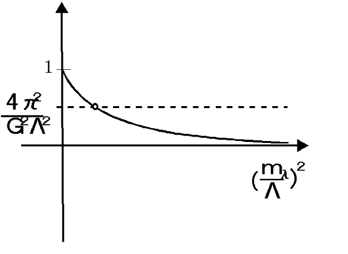
Figure 6: Left hand side of eq.(3.42)(dotted line) and right hand side(solid line) is plotted. If the four-fermi coupling is strong enough, non-trivial solution appears.

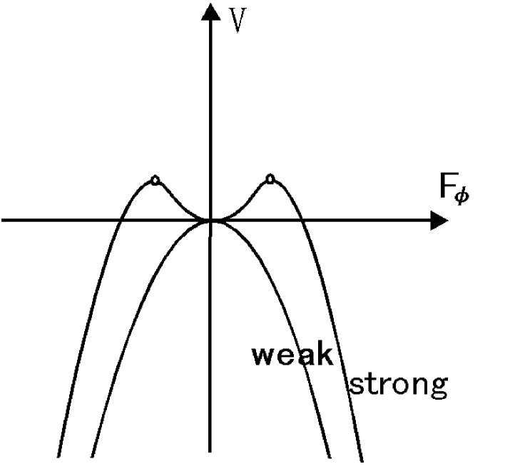
Figure 7: The relation between $F_{\phi}$ and the scalar potential is plotted for the weak and the strong coupling phases of massless SQCD with $N_{f}<N_{c}-1$. The explicit form of this potential is not calculated explicitly, but the stationary point of this potential is already calculated in (3.41). The solution for the gap-equation always lies at the stationary point of this potential. Because $F_{\phi}$ is an auxiliary field, the form of the potential is not important.

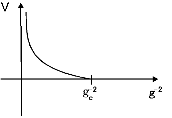
Figure 8: The explicit 1-loop potential for massless SQCD with $N_{f}<N_{c}-1$. Asymptotic behavior is different from the effective Lagrangian analysis. We are not sure whether this difference comes from an artificial reason or there is really a phase transition for gaugino condensation. In pure supersymmetric Yang-Mills theory, we have good reasons to believe that there is no phase transition and gaugino condensates for any value of $g$, but in this case it is very difficult to examine.

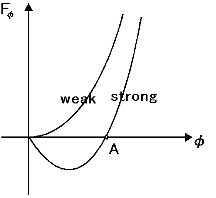
Figure 9: The relation between $F_{\phi}$ and $\phi$ for SQCD with small mass term is plotted. It is obvious that we can find a supersymmetric vacuum state with vanishing $F_{\phi}$.

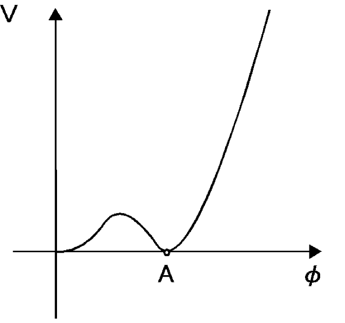
Figure 10: The explicit form of scalar potential is plotted for the weakly and the strongly coupled phases. We can find a “stable” supersymmetric vacuum state.

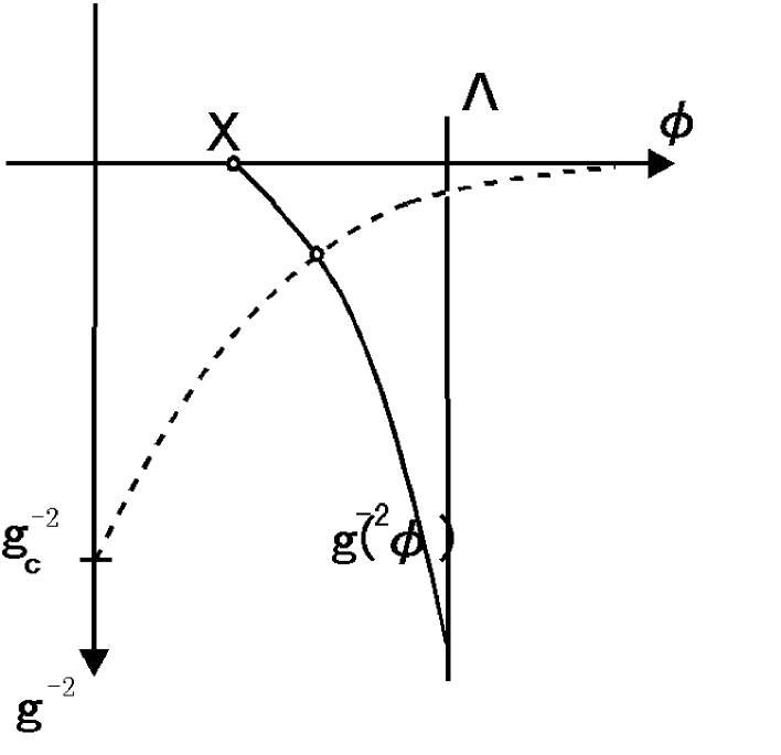
Figure 11: The dotted line presents the solution A in Fig.9 and Fig.10 for arbitrary $g$. This line is obtained by solving the equation (3.45) with the assumption that $g$ does not depend on $\phi$. (See also eq.(3.42) and fig.6) The solid line shows the relation between $g$ and $\phi$. To find a true vacuum, we should find a point at which both of these two lines meet. Seeing this graph, we can easily understand why no phase transition is observed in massive SQCD. In general, we tend to think that the vacuum lies at $X$, which corresponds to a solution for $f(\varphi)=0$.

3.3 Summary of section 3

In the first half of this section we have reviewed ref.[27] as an introduction to the dynamical analysis of supersymmetric QCD. In the latter half, we considered a new method for the analysis of gaugino condensation and the generation of the non-perturbative potential. Our analyses are almost consistent with the previous ones. Moreover, a non-trivial assumption, that was made in [27], is examined. In the large N limit we have shown that the phase transition of gaugino condensation does not occur in massive case but does occur in massless case.

4 Dynamical analysis in supergravity theories

In general, one may think there are four different ways of introducing gaugino condensates into supergravity.

First, in the component Lagrangian method[32], one takes the standard Lagrangian of supersymmetric Yang-Mills theory coupled to supergravity and replaces the gaugino bilinear with a constant of the order of the condensation scale $\mu^{3}$. Such a procedure has the drawback of discarding the back-reaction of other fields, hence one cannot determine in this way whether the condensate really forms. The formation of the condensate and its magnitude here are simply assumed implicitly relying on the observation made in the global version of the model. However, as we have assumed that gravitational corrections can play an important role, the internal consistency of this approach is not clear.(There is no reason to believe that dynamical properties of the global supersymmetric models are not changed in supergravity models.)

Second, a refinement of this approach is considered[11]. Taking into account a possible dependence of condensate on some fields leads to the superpotential method. Using these one can then construct the gaugino induced non-perturbative corrections to the original superpotential of the model. For example, the belief that the condensate dissolves in the weak coupling limit leads to a superpotential which decays exponentially with the increasing value of the dilaton field. One may then search for minima of the effective theory and determine the true value of the gaugino condensate that leads to the supersymmetry breaking in supergravity theories.

The third method is the effective Lagrangian approach[9]. Generalizing the global effective potential written by the composite superfields, one can obtain the supergravitational version of the effective potential which is of course consistent to the global theory in the $M_{p}\rightarrow\infty$ limit. In supergravity models the effective scalar potential is:

$$V=g_{ij^{*}}F^{i}F^{j^{*}}-3e^{G}$$ (4.1)

where $G=K+log(|W|^{2})$ and $g_{ij^{*}}=\partial^{2}K/\partial z^{i}\partial z^{j^{*}}$.

The fourth method is the Nambu-Jona-Lasinio like approach first developed by G.G.Ross et al[33]. One of the major advantages of this method is the clear relation between the constituent Lagrangian and the effective Lagrangian with gaugino condensation. The driving force, that makes gaugino condensate as the coupling becomes strong, is now clear. The stability of the moduli potential is also modified, which we think as another advantage of this method.

4.1 Review of the general analysis

There has recently been considerable attention focused on the study of supersymmetric models of elementary particle interactions. This is especially true in the context of grand unification theories, where remarkable studies have been done in the hope of solving the gauge hierarchy problem or unifying the gravitational interaction within the superstring formalism. Supersymmetric extension of the gravity(supergravity) seems necessary when one introduces soft breaking terms and makes the cosmological constant vanish at the same time. In supergravity models, spontaneous breaking of local supersymmetry or super-Higgs mechanism may generate soft supersymmetry breaking terms that allow to fulfill such phenomenological requirements. However, the super-Higgs mechanism implies the existence of a supergravity breaking scale, intermediate between the Planck scale($M_{p}$) and the weak scale($M_{W}$). The intermediate scale is expected to be of O($10^{13}$Gev). Here we expect that this intermediate scale is implemented by the mechanism of gaugino condensation in the hidden sector which couples to the visible sector by gravitational interactions. The effective action for gaugino condensation is well studied by many authors[5, 31].

Before discussing the large N expansion of supergravity, we will review the general approaches to the dynamical properties. In this section, we mainly follow ref.[31] and study gaugino condensation in the hidden sector in a modular invariant way. Gaugino condensation is, in general, believed to be a potential source of hierarchical supersymmetry breaking and the source of a non-trivial potential for the dilaton $S$, whose real part corresponds to the tree level gauge coupling constant. In the effective Lagrangian approach, however, we cannot find a stable potential for dilaton without introducing multiple gaugino condensations. However, if we include hidden matter fields with multiple hidden gauge groups, we can obtain a reasonable value for $S$ and soft breaking terms.

First we consider gaugino condensation without matter fields. the strategy is as follows.

• Derive the general form of the corresponding scalar potential and the minimization conditions.

• Consider in a separate way the case of one, two or more gaugino condensations.

(Multiple gaugino condensation can lead to a stable dilaton potential, but to produce realistic soft terms we need some extensions, for example, inclusion of hidden matter fields. In this sense, hidden matter fields are necessary for realistic model building.)

The process of gaugino condensation in the context of a pure Yang-Mills N=1 supergravity theory has been pretty well understood for a long time. It can be described conveniently by an effective superpotential $W^{np}(U)$ of the chiral composite superfield $U$ whose scalar component corresponds to the gaugino composite bilinear field. Assuming that the form of $W^{np}$ is the same as pure supersymmetric Yang-Mills theory, $W^{np}$ reads:

$$W^{np}=aU(f+\frac{2}{3}\beta logU)$$ (4.2)

Here $a$ is some constant. In this case $f$ would be modular dependent and may contain the threshold corrections from underlying string theory. As has been demonstrated in refs.[[36, 37, 38]], it is equivalent to work with the explicit form of $W^{np}$(4.2) or with the resulting superpotential after substituting the minimum condition $\partial W^{np}/\partial U=0$:

$$W^{np} = de^{\frac{3}{2\beta}f}$$ (4.3)

$$= d\frac{e^{\frac{-3kS}{2\beta}}}{\Pi^{3}_{i=1}[\eta(T_{i})]^{2-\frac{3k}{4\pi^{2}\beta}\delta^{GS}_{i}}}$$

where $d=-\beta/6e$. If the gauge group is not simple, i.e.$G=\Pi_{a}G_{a}$, then $W^{np}=\sum_{a}W^{np}_{a}$. Now the scalar potential is given by:

$$V = \frac{2}{Y\Pi^{3}_{i=1}T_{Ri}}\left[|YW_{S}-W|^{2}\frac{}{}\right.$$ (4.4)

$$+\sum^{3}_{i=1}\frac{Y}{Y+\frac{1}{4\pi^{2}}\delta^{GS}_{i}}\left|(W+\frac{1}{4\pi^{2}}\delta^{GS}{i}W_{S})-\frac{1}{2}T_{Ri}W_{T_{i}}\right|^{2}$$

$$\left.-3|W|^{2}\right]$$

Using this scalar potential and numerical methods, the property of the vacuum state was studied. Here we only show the results of the previous papers[31]

• With simple gauge group
  In this case, we cannot find the stable vacuum state. The asymptotic minimum appears at infinity, that is called “runaway vacuum”.

• With multiple gauge groups
  If $k_{a}$ is different from each other, we can find a stable minimum. However, such a vacuum does not have phenomenologically acceptable values of moduli fields.

• With hidden matters with multiple gauge groups
  Including multiple hidden matter fields, we can obtain a phenomenological vacuum state. But one should not think that the inclusion of hidden matter is essential, because such an extra parameter region generally makes it easy to adjust the vacuum parameters by hand.

4.2 Large N expansion

Now we use large N expansion to analyze the vacuum state of supergravity theories. The extension from the previous analysis (analysis for global models) is straightforward.

4.2.1 Introduction

In the previous section we have analyzed the large N expansion and gap-equations for global supersymmetric models. The key idea of the analysis was to consider an intermediate scale effective Lagrangian which couples to R-axion superfield.

In this section, we extend the analysis of global supersymmetric models with R-symmetry to its local version with Weyl symmetry. This Weyl symmetry is always present when one consider the superstring inspired models and this symmetry needs a compensator superfield. This compensator plays almost the same role as R-symmetry compensator in the global models.

4.2.2 Gaugino condensation in supergravity

In the standard superfield formalism of the locally supersymmetric action, we have the Lagrangian:

$$S = \frac{-3}{\kappa^{2}}\int d^{8}zEexp\left(-\frac{1}{3}\kappa^{2}K_{0}\right)$$ (4.5)

$$+\int d^{8}z{\cal E}\left[W_{0}+\frac{1}{4}f_{0}{\cal WW}\right]+h.c.$$

Here we set $\kappa^{2}=8\pi/M_{p}^{2}$. In the usual formalism of minimal supergravity, the Weyl rescaling is done in terms of component fields. However, in order to understand the anomalous quantum corrections to the classical action, we need a manifest supersymmetric formalism, in which the Weyl rescaling is also supersymmetric. It is easy to see that the classical action(4.5) itself is not super-Weyl invariant. However, the super-Weyl invariance can be recovered with the help of a chiral superfield $\varphi$(Weyl compensator).

For the classical action (4.5), the Kähler function $K_{0}$, the superpotential $W_{0}$ and the gauge coupling $f_{0}$ are modified in the following way[34]:

$$K_{0} \rightarrow K=K_{0}-6\kappa^{-2}{\sf Re}log\varphi$$

$$W_{0} \rightarrow W=\varphi^{3}W_{0}$$

$$f_{0} \rightarrow f=f_{0}+\xi log\varphi$$ (4.6)

$\xi$ is the constant which is chosen to cancel the super-Weyl anomaly. The super-Weyl transformation contains an R-symmetry in its imaginary part, so we can think that this is a natural extension of [33] in which a compensator for the R-symmetry played a crucial role in obtaining the gap equation.

Let us examine the simplest case. We include some scale factor $\Lambda$ and set the form of $W_{0}$ and $f_{0}$ as:

$$W_{0} = \lambda\Lambda^{3}$$

$$Ref_{0} = \frac{1}{g^{2}_{0}}$$ (4.7)

and rescale the field $\varphi$ as:

$$\tilde{\varphi}=\Lambda\varphi$$ (4.8)

Finally we have:

$$K = K_{0}-6\kappa^{-2}{\sf Re}log\left(\frac{\tilde{\varphi}}{\Lambda}\right)$$

$$W = \lambda{\tilde{\varphi}}^{3}$$

$$f = \frac{1}{g^{2}_{0}}+\xi log\left(\frac{\tilde{\varphi}}{\Lambda}\right)$$ (4.9)

The sign of $\lambda$ should respect the condition $\lambda\xi>0$ so that the gap-equation can develop non-trivial solution. We can obtain a constraint equation from the equation of motion for the auxiliary component $h_{\varphi}$ of the super-Weyl compensator. The relevant part of the Lagrangian is:

$$e^{-1}L_{AUX}=\left[\frac{\partial W}{\partial\varphi}-\frac{1}{4}\frac{\partial f}{\partial\varphi}\lambda\lambda\right]h_{\varphi}$$ (4.10)

From the equation of motion, constraint is now written as:

$$\frac{\partial W}{\partial\varphi}=\frac{1}{4}\frac{\partial f}{\partial\varphi}\lambda\lambda$$ (4.11)

for the rescaled field, this can be written as:

$$\lambda\tilde{\varphi}^{3}-\frac{\xi}{12}g^{2}\lambda^{\alpha}\lambda_{\alpha}=0$$ (4.12)

The tree level scalar potential for this minimal model is:

$$V_{0} = -3\kappa^{2}|W|^{2}$$ (4.13)

$$= -3\kappa^{2}\lambda^{2}|\tilde{\varphi}^{3}|^{2}$$

The equation of motion for the auxiliary field(4.12) suggests that eq.(4.13) can be interpreted as a four-fermion interaction of the gaugino:

$$-\frac{1}{48}\kappa^{2}g^{4}\xi^{2}|\lambda^{\alpha}\lambda_{\alpha}|^{2}$$ (4.14)

This four-fermion interaction becomes strong as $\frac{1}{g^{2}}={\sf Re}f$ reaches 0. The strong coupling point is:

$$\tilde{\varphi}_{s}=\Lambda e^{-\frac{1}{g^{2}_{0}\xi}}$$ (4.15)

In the effective Lagrangian analysis, one usually assumes that this point is the true vacuum. We show the vacuum state of three types of analysis(effective Lagrangian analysis, G.G.Ross type and large N expansion) in Fig.(13).

By using the tadpole method we can obtain a gap equation:

$$\lambda\tilde{\varphi}^{3} \times \left(1-4G^{2}\int\frac{d^{4}p}{(2\pi)^{4}}\frac{1}{p^{2}+m_{\lambda}^{2}}\right)=0$$ (4.18)

$$\left\{\begin{array}[]{l}G^{2}=\frac{\xi^{2}\kappa^{2}g^{4}n_{g}}{12}\\ m_{\lambda}^{2}=\frac{\kappa^{4}\xi^{2}g^{4}\lambda^{2}|\tilde{\varphi}^{3}|^{2}}{4}\end{array}\right.$$

where $\xi$ is determined by the anomaly constraint and $n_{g}$ is the dimension of the gauge group($n_{g}=N_{c}^{2}-1$). Here, it is proportional to $N_{c}$. This equation is a good approximation when we take $N_{c}\rightarrow\infty$ limit. (The leading contribution is enhanced by an extra $N_{c}$ factor. See fig.(12)

The solution for the gap equation(4.18) is plotted in Fig.(13). We can see that there is always a solution for non-zero gaugino condensation. Now let us consider the difference between our result and ref.[33]. In ref.[33], the solution for the gap equation is estimated after fixing the coupling constant at $g_{c}$ which is introduced by hand. It is true that the effective potential is singular at $\tilde{\varphi}_{s}$ (4.15), but without introducing the cut-off for the strength of the four fermion coupling $|\lambda\lambda|^{2}$, we can find a stable solution for (4.18) at finite value.(see Fig (13))

For a second example, we include the dilaton superfield $S$. Now $f_{0}$ is not a constant and depends on the field $S$:

$$f_{0}=S$$ (4.19)

And the Kähler potential for the dilaton superfield is:

$$K_{0}=-\kappa^{-2}log(S+\overline{S})$$ (4.20)

Here we should include the effect of the dilaton field in the scalar potential. The tree level scalar potential is:

$$V_{0}=h_{S}(G^{-1})^{S}_{S}h^{S}-3\kappa^{2}|W|^{2}$$ (4.21)

The auxiliary field for $S$ is:

$$h_{S} = \kappa^{2}\left[\frac{1}{2}\frac{W}{S+\overline{S}}+\frac{1}{4}f_{S}\lambda^{\alpha}\lambda^{\alpha}\right]$$ (4.22)

$$= \frac{\kappa^{2}}{4}W\frac{1+12S_{R}\xi^{-1}}{S_{R}}$$

Here we set $G=K+ln(\frac{1}{4}|W|^{2})$ and $S_{R}=(S+\overline{S})/2$. The tree level potential can be given in a simple form

$$V_{0}=\lambda^{2}A|\tilde{\varphi}^{3}|^{2}$$ (4.23)

where

$$A=\frac{1}{16}\kappa^{2}\left[\left(1+\frac{12S_{R}}{\xi}\right)^{2}-3\right].$$ (4.24)

The tree level potential for $\tilde{\varphi}$ has no stable supersymmetry breaking solution. This is consistent with an observation that gaugino condensation as usually parameterized does not occur in models with a single gauge group in the hidden sector. However, we have argued that it is essential to go beyond tree level to include non-perturbative effects in the effective potential which may allow non-trivial minimum even in the simplest case of a single hidden sector gauge group. This non-perturbative sum is readily obtained by computing the one-loop correction to $V$, or directly from the gap-equation. In this case, the gap equation is given by the same constraint equation (4.12), but gaugino mass term is modified.

$$\lambda\tilde{\varphi}^{3} \times \left(1-4G^{2}\int\frac{d^{4}p}{(2\pi)^{4}}\frac{1}{p^{2}+m_{\lambda}^{2}}\right)=0$$ (4.28)

$$\left\{\begin{array}[]{l}G^{2}=\frac{\lambda g^{4}\xi^{2}g^{4}n_{g}A}{24}\\ m_{\lambda}^{2}=\frac{A^{2}\xi^{2}g^{4}\lambda^{2}g^{2}|\tilde{\varphi}^{3}|^{2}}{36}\\ n_{g}=N_{c}^{2}-1\end{array}\right.$$

This equation is, however, too complicated to find a solution. We thus forced to employ some simplification of this analysis, for example, fix the four-fermi interaction coefficient[33] or to approximate the solution at which $g^{2}$ goes to infinity, i.e. $f(S)=0$[31]. Here we only refer to the paper[33] in which the stability of the potential is well discussed after fixing the four-fermi interaction coefficient. In [33], duality invariant Lagrangian is also considered and it is found that this type of approach takes into account some additional non-perturbative effects [35] and stabilizes the dilaton potential with only one gauge group.

To see the basic mechanism involved, let us reconsider eq.(4.23). This potential suggests that, once gaugino condensate and $\varphi$ gets non-zero value, $S$ cannot run away to infinity. On the other hand, it is obvious from fig.(13) that eq.(4.28) always have non-trivial (condensating) solution for any $S$. Moreover, in the effective Lagrangian analysis one consider that the point C in fig.(13) is the solution for non-trivial gaugino condensation. As $S$ becomes large, C moves toward the origin as the function of $e^{-S}$ so one tends to think that the potential (4.23) is destabilized. On the other hand, if one uses Nambu-Jona-Lasinio type approach[33], one is lead to the solution B in fig.(13) and finds that the potential is indeed stable. However, taking large N limit, we can find that these two solutions corresponds to different kinds of approximations for the true solution at A, which is different from both B and C. Because the solution A is very similar to the solution B and does not behave as $e^{-S}$, we may think that the potential is stabilized at the true vacuum A.

4.3 Summary of section 4

In this section we have considered the analysis of the non-perturbative properties of supergravity theory which is induced by low energy dynamics of gaugino condensation. After a brief review of the previous approaches, we examined these known results from another point of view. By using large N expansion, we showed that the effective Lagrangian analysis and Nambu-Jona-Lasinio type approach can be regarded as different kinds of approximations to the exact solution.

In the large N limit, we can easily understand why the dilaton potential is stabilized in Nambu-Jona-Lasinio type approach but not stabilized in the effective Lagrangian approach. We also found a stable and exact solution in the large N limit. It is important that we can find a stabilized dilaton potential if we take into account a certain non-perturbative effect from supergravity.

Figure 12: The gap equation (4.23) is written in a diagrammatic form. One of the typical higher correction is shown in the second diagram.

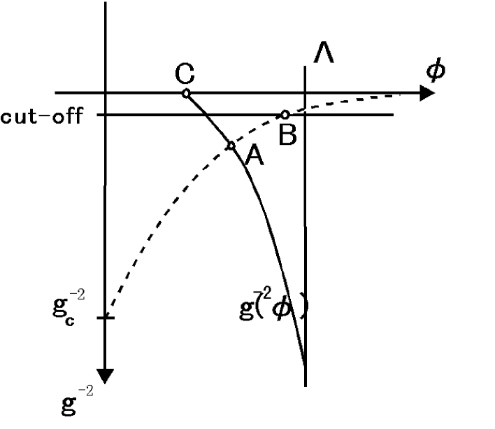
Figure 13: The stationary point of the scalar potential(dotted line) and the relation between $g$ and $\varphi$ (solid line) are plotted in the same graph. The only “exact” solution lies at A. If we include a cut-off for the four-fermi interaction coefficient by hand, we will find a vacuum at B(see Appendix). C is the strong coupling point, where $Ref$ vanishes and the gauge coupling $g$ goes to infinity. In many cases, we use C for the solution for the non-trivial gaugino condensation(The relation between effective potential analysis and the condition $f=g^{-2}=0$ is well discussed in ref.[34]).

5 Conclusions and discussions

In this paper, we have given a systematic study of the dynamical properties of supersymmetric theories by using the large N expansion.

First we have analyzed the O(N) non-linear sigma model as the simplest and explicitly solvable example. All the parameters are determined exactly and no ambiguities are left. We have also examined the effects of the supersymmetry breaking mass term on the dynamical properties.

For the second example, we have studied supersymmetric QCD with $N_{f}<N_{c}-1$. What we have been concerned with was the condensation of gaugino which can be viewed as the source of the non-perturbative superpotential. Large N expansion is realized in the limit of $N_{f}\rightarrow\infty$ while $N_{c}-N_{f}$ is fixed. The results almost coincide with the previous analyses[5, 27]. We have examined a non-trivial assumption on phase transition for gaugino condensation that was made in ref.[27] and given alternative proof for it. We have proved in the large N limit that no phase transition is allowed for gaugino condensation in massive SQCD. However, in massless SQCD, phase transition does occur in the weak coupling region. This can change the asymptotic form of the runaway potential. To be more precise, the flat directions are only partially lifted and does not run away.

For the third example, we have analyzed superstring motivated supergravity theories which is the main theme of our paper. In the large N limit, we found that the analyses derived from effective (confined) theory[31] and one from Nambu-Jona-Lasinio type approach[33] correspond to the different kinds of approximations for the exact solution. (This is explicitly visualized in fig.(13).) We have used the constituent fields. This type of approach is very important when we think of the phenomenological implications of supersymmetry breaking mechanism on the moduli stabilization[35] and the phase transitions in the early universe[39]. As is discussed in ref.[35], one should discard important part of the non-perturbative effects from supergravity if he considers only a composite type Lagrangian that should be obtained by merely turning off the supergravity effects.

Appendix A Review of the approach by G.G.Ross et al

In this appendix we review the series of papers written by G.G.Ross et al[33]. The main idea of their analysis comes from an effective low-energy (still not confined) theory describing the Goldstone mode associated with the R-symmetry breaking driven by gaugino condensation. This theory has four-fermi interaction at the tree level and they examined its implications to gaugino condensation a la Nambu-Jona-Lasinio type approach.

First, let us construct the Lagrangian. Demanding that the effective theory given in terms of the auxiliary field $\Phi$ generates four-fermion interaction then the form of the $W$ and $f$ are determined.

$$W = m^{2}\Phi$$ (A.1)

$$f = \xi ln(\Phi/\mu)+S$$ (A.2)

where $m$ and $\mu$ are mass parameters, $\xi$ is a dimensionless constant and $S$ is a dilaton superfield. Here we take $M_{p}=1$ for simplicity. The classical equation of motion for auxiliary component of $\Phi$ ($\phi,\chi,h$) is:

$$\frac{1}{2}\frac{\partial W}{\partial\phi} = \frac{e^{K/2}}{4}\frac{\partial f}{\partial\phi}\lambda\lambda$$ (A.3)

This gives the relation:

$$\phi=\frac{e^{K/2}\xi}{2m^{2}}\lambda\lambda$$ (A.4)

which means that the field $\phi$ can be an order parameter for gaugino condensation. The four-fermion term appears if we consider the tree level (supergravity) potential:

$$V_{0}=3e^{-G}+h_{S}f^{S}(G^{-1})^{S}_{S}$$ (A.5)

where $h_{S}$ denotes the F-component of the chiral superfield $S$ given by:

$$h_{S}=e^{-G/2}G_{S}+\frac{1}{4}\lambda\lambda-G^{jk}_{S}\overline{\chi}_{j}\chi_{k}-\frac{1}{2}\overline{\chi}_{S}G_{j}\chi^{j}$$ (A.6)

Including all the components, we can write the tree level potential explicitly:

$$V_{0} = \frac{1}{4}\left(1+\frac{S+\overline{S}}{\xi}\right)^{2}e^{-K}|W|^{2}$$ (A.7)

$$= \frac{1}{4}\left(1+\frac{S+\overline{S}}{\xi}\right)^{2}e^{-K}m^{4}\phi^{2}$$

In terms of gaugino field, we can obtain the four-fermion interaction term.

$$L_{4fermi}=\frac{1}{16(Ref)^{2}}\left(1+\frac{S+\overline{S}}{\xi}\right)^{2}|\lambda\lambda|^{2}$$ (A.8)

where the factor of $Ref$ in the denominator appears because we have rescaled the gaugino fields appearing in this equation to have canonical kinetic terms.

The form we have derived depends on the parameters $\xi$, $m$ and $\mu$. One can determine $\xi$ by demanding that the low-energy effective Lagrangian is anomaly free under the R-symmetry transformation. The mass scale $m$ should be identified with the Planck mass. Different choices of $\mu$ are possible and we take $\mu=\Lambda^{3}_{GUT}/m_{Planck}^{2}$. This choice of $\mu$ is justified in superstring motivated analysis. A supersymmetry breaking solution to the mass gap $\partial(V_{0}+V_{1})/\partial\phi=0$ is dynamically favored for a large coupling constant. The apparent singularity when $Ref$ approaches zero and the potential unbounded from below are not physically reasonable. On dimensional grounds we introduce a cut-off at the scale $Ref=\Lambda_{c}$ which corresponds to the effective four-gaugino interaction $|\lambda\lambda|^{2}/\Lambda_{c}^{2}$. (See Fig.(13).)

We can easily extend this model to include other moduli fields and string threshold corrections. Here we give the explicit form of typical Lagrangian:

$$K = -ln\left(S_{R}+2\sum_{i}k_{a}\delta^{i}_{GS}lnT_{Ri}\right)-\sum_{i}lnT_{Ri}$$

$$W = W_{0}+W_{m}$$

$$f_{0} = S+2\sum_{i}(b_{a}^{{}^{\prime}i}-k_{a}\delta^{i}_{GS})ln[\eta(T_{i})]^{2}$$ (A.9)

where $W_{0}$ is the scalar potential due to the gaugino condensate and $W_{m}$ is the matter superpotential.

If we demand that the effective theory given in terms of the auxiliary superfield $\Phi$ generates four-fermi interaction then the form of the $W$ and $f$ are uniquely determined.

$$W_{0} = m^{2}\Pi_{i}\eta^{-2}(T_{i})\Phi$$

$$f = f_{0}+\xi ln\frac{\Phi}{\mu}$$ (A.10)

From the classical equation of motion the scalar component of the auxiliary superfield $\Phi$ is given in terms of the gaugino bilinear by:

$$\phi=\frac{e^{-K/2}\xi}{2m^{2}\Pi_{i}\eta^{-2}_{i}}\lambda\lambda$$ (A.11)

For a pure gauge theory in the hidden sector the tree level scalar potential is now written by:

$$V_{0} = m^{2}_{\frac{3}{2}}B_{0}$$

$$B_{0} = \left(1+\frac{Y}{\xi}\right)^{2}+\sum_{i}\frac{Y}{Y+a_{i}}\left(a_{i}-\frac{a_{i}}{\xi}\right)^{2}\frac{T_{Ri}}{4\pi^{2}}|G_{2}(T_{i})|^{2}-3$$ (A.12)

where $G_{2}$ is the Einstein modular form with weight $1/2$ and $a_{i}$ is defined as $a_{i}=2(k_{a}\delta^{GS}_{i}-b^{{}^{\prime}}_{ai})$. The gravitino mass is given by:

$$m_{\frac{3}{2}}=\frac{1}{4}e^{K}\Pi_{i}|\eta(T_{i})|^{-4}|\phi|^{2}$$ (A.13)

It is clear that a non-zero gravitino mass is only possible for non-vanishing VEV of $\phi$. The one-loop radiative corrections may be calculated using Coleman-Weinberg one-loop effective potential.

$$V_{1}=\frac{1}{32\pi^{2}}Str\int d^{2}pp^{2}ln(p^{2}+M^{2})$$ (A.14)

After introducing the cut off parameter for $Ref$ and fixing the form of four-fermion interaction term as $|\lambda\lambda|^{2}/\Lambda_{c}^{2}$, the extremum conditions are solved.

Here we do not describe further detailed analysis on this phenomenological applications because our aim in this appendix is to introduce a main idea of the method developed by G.G.Ross et al.

References

- [1] H.P.Nills, Phys.Rep.110(1984)1
- [2] S.Deser and B.Zumino, Phys.Rev.Lett.38(1977)1433
- [3] M.Dine, A.E.nelson, Y.Shirman, Phys.Rev.D51(1995)1362
-
[4]
J.Wess and J.Bagger, Supersymmetry and Supergravity (1992)
Princeton University press -
[5]
D.Amati, K.Konishi, Y.Meurice, G.C.Rossi, G.Veneziano,
Phys.Rep.162(1988)169 - [6] E.Witten, Nucl.Phys.B188(1981)513;Nucl.Phys.B202(1982)253
- [7] H.P.Nills, Phys.Rev.Lett.115(1982)193
- [8] N.V.Krasnikov, Phys.Lett.B193(1987)37
-
[9]
J.A.Casas, Z.Lalak, C.Munoz and G.G.Ross,
Nucl.Phys.B347(1990)243;
J.A.Casas, Z.Lalak and C.Munoz, Nucl.Phys.B399(1993)623 -
[10]
M.B.Green and J.H.Schwarz and E.Witten, Superstring Theory (1987)
Cambridge Univ. Press -
[11]
M.Dine, R.Rohm, N.Seiberg and E.Witten,
Phys.Lett.B156(1985)55 -
[12]
G.D.Coughlan, G.Germain, G.G.Ross and G.Segreé
Phys.Lett.B198(1987)465;
P.Binétury and M.K.Gaillard, Phys.Lett.B253(1991)119;
Z.Larak, A.Niemeyer, G.Girald and R.Grimm,
Nucl.Phys.B453(1995)100 -
[13]
S.Kachru, hep-th/9603059
E.Witten, hep-th/9604030
K.R.Dienes and A.E.Faraggi, Phys.Rev.Lett.75(1995)2646 - [14] T.Matsuda, J.Phys.A28(1995)3809
- [15] K.Fujikawa and W.Lang, Nucl.Phys.B88(1975)61
- [16] T.Matsuda, J.Phys.G22(1996)1127
- [17] T.Matsuda, J.Phys.G22(1996)119
- [18] D.J.Gross, A.Neveu, Phys.Rev.D10(1974)3235
- [19] A.M.Polyakov, Phys.Lett.59B(1975)79
- [20] E.Witten, Phys.Rev.D16(1977)2991
-
[21]
A.C.Davis, P.Salomonson, J.W.Holten,
Nucl.Phys.B208(1982)484 - [22] O.Alvarez, Phys.Rev.D17(1978)1123
-
[23]
A.M.Polyakov Gauge Fields and Strings,
Harwood Academic Publishing(1987) -
[24]
S.Weinberg, Phys.Rev.D7(1973)2887
R.Miller, Phys.Lett.124B(1983)59; Nucl.Phys.B241(1984)535
- [25] V.G.Koures, K.T.Mahathappa, Phys.Rev.D43(1991)3428
-
[26]
O.Aharony, J.Sonnenschein, M.E.Peskin and S.Yankielowicz,
Phys.Rev.D52(1995)6157
L. Alvarez-Gaume, M. Marino,hep-th/9606168
-
[27]
I.Affleck, M.Dine, N.Seiberg,
Nucl.Phys.B241(1984)493;Nucl.Phys.B256(1985)557
- [28] J.Polchinski, Phys.Rev.D26(1982)3674
- [29] T.Matsuda, J.Phys.G22(1996)L29
- [30] T.Matsuda, Phys.Rev.D54(1996)7650
-
[31]
J.P.Derendinger, L.E.Ibàñez and H.P.Nills,
Phys.Lett.B155(1985)65
M.Dine, R.Rohm, N.Seiberg and E.Witten, Phys.Lett.B156(1985)55
C.Kounnas and M.Porrati, Phys.Lett.B191(1987)91
S.Ferrara, N.Magnoli, T.R.Taylor and G.Veneziano,
Phys.Lett.B245(1990)243
A.Font, L.E.Ibàñez, D.Lust and F.Quevedo, Phys.Lett.B245(1990)401
H.P.Nills and M.Olechwski, Phys.Lett.B248(1990)268
P.Binètury and M.K.Gaillard, Phy.Lett.B253(1991)119;
Nucl.Phys.B358(1991)194
B.de Carlos, J.A.Casas and C.Muñoz, Nucl.Phys.B399(1993)623 - [32] S.Ferrara, L.Girardello and H.P.Nills, Phys.Lett.125B(1983)457
-
[33]
A.de la Maccora and G.G.Ross,
Nucl.Phys.B404(1993)321; Phys.Lett.B325(1994)85;
Nucl.Phys.B443(1995)127 - [34] V.Kaplunovsky and J.Louis, Nucl.Phys.B422(1994)57
- [35] B. De Carlos and M. Moretti, Phys.Lett.B341(1995)302
- [36] J.A.Casas, Z.Lalak, C.Munoz and G.G.Ross, Nucl.Phys.B347(1990)243
- [37] D.Lust and T.R.Taylor, Phys.Lett.B253(1991)335
- [38] B.de Carlos, J.A.Casas and C.Munoz, Phys.Lett.B263(1991)248
- [39] T.Matsuda,Phys.Lett.B383(1996)28