Masses, Decays and Mixings of Gluonia in QCD

S. Narison
Laboratoire de Physique Mathématique et Théorique
Université de Montpellier II
Place Eugène Bataillon
34095 - Montpellier Cedex 05, France
Abstract

We compute the masses and decay widths of the gluonia using QCD spectral sum rules and low-energy theorems. In the scalar sector, one finds a gluonium having a mass $M_{G}=(1.5\pm 0.2)$ GeV, which decays mainly into the $U(1)_{A}$ channels $\eta\eta^{\prime}$ and $4\pi^{0}$. However, for a consistency of the whole approach, one needs broad-low mass gluonia (the $\sigma_{B}$ and its radial excitation), which couple strongly to the quark degrees of freedom similarly to the $\eta^{\prime}$ of the $U(1)_{A}$ sector. Combining these results with the ones for the $\bar{q}q$ quarkonia, we present maximal gluonium-quarkonium mixing schemes, which can provide quite a good description of the complex spectra and various decay widths of the observed scalar mesons $\sigma(1.),~{}f_{0}(0.98),~{}f_{0}(1.37),~{}f_{0}(1.5)$ and $f_{J}(1.71)$. In the tensor sector, the gluonium mass is found to be $M_{T}\simeq(2.0\pm 0.1)$ GeV, which makes the $\zeta(2.2)$ a good $2^{++}$ gluonium candidate, even though we expect a rich population of $2^{++}$ gluonia in this region. In the pseudoscalar channel, the gluonium mass is found to be $M_{P}\simeq(2.05\pm 0.19)$ GeV, while we also show that the $E/\iota$(1.44) couples more weakly to the gluonic current than the $\eta^{\prime}(0.96)$, which can favour its interpretation as the first radial excitation of the $\eta^{\prime}$(0.96).

PM 96/37

hep-ph/9612448

December 1996

1 Introduction

There is now clear evidence from many processes that QCD is the theory of strong interactions. All hard processes satisfy the asymptotic freedom property of QCD, while the complicated hadron properties can be explained by different non-perturbative methods (effective Lagrangian, lattice calculations, QCD spectral sum rule (QSSR),…). However, in addition to the well-known mesons and baryons bound states, one of the main consequences of the QCD theory is the possible existence of the gluon bound states (gluonia or glueballs) or/and of a gluon continuum. The theoretical interest in the gluonia sector has started a long time ago, since the pionneering work of Fritzsch and Gell-Mann [1], as shown by the long list of publications on this topic. However, despite these different efforts, the theoretical and experimental status remains unclear. From the theoretical point of view, this is due to our poor control of the gluon dynamics. In particular, there is not yet any convincing dynamical approach that computes the mixing of the gluonia with quarkonium states (see however [2, 3]), which is necessary if one wishes to make contact with the experimental data. At this level, only phenomenological scheme is available, where the mixing angle is only fitted from the data. From the experimental point of view, the difficulty also arises in the same way, as the observed resonances can be a mixing between gluonia and quarkonia. However, some selected processes such as the $J/\psi$ radiative decays can favour more the production of gluonia than of quarkonia, while the measurement of the two-photon widths has been used for a long time as a good gluonia signature. However, as proposed some years ago in [4], a good signature for the presence of the gluonia can be obtained from the ratio of the previous two quantities referred to as “stickiness”. Another possibility for signing the nature of an almost pure gluonium is the measurements of its width into the U(1)-like channels: $\eta^{\prime}\eta^{\prime}$, $\eta\eta^{\prime}$, and $4\pi^{0}$, which are expected to be more dominant than, for instance, the one into pair of pions, leading [5, 6] to the conclusions that the G(1.6) observed by the GAMS group [7] is an almost pure glueball state. The different experimental progress done during these last few years [8], though not yet very conclusive , is encouraging for improving the theoretical predictions. Some recent efforts have been accomplished in this direction from lattice calculations [9]–[11]. However, the “apparent” disagreements of these lattice results can simply reflect the true systematic error of the estimates from this approach. Recently, some QCD inequalities among the gluonia masses have been derived [12]. Some qualitative phenomenological attempts [13] have also been proposed for explaining the nature of the scalar meson seen by the Crystal Barrel collaboration [14]. Motivated by these different steps forward, we plan to give in this paper an almost complete scheme and an update of the predictions from QSSR à la SVZ [15] , where, in my opinion, the results have often been misinterpreted in the literature, and in some cases ignored. A long list of sum rules results exists in the literature [17]–[26], which needs to be updated because of the progress accomplished in QCD during the last few years. This is the aim of this work. The paper is organized as follows:
In section 2, we give a general discussion on the gluonia and the classification of different currents. In section 3, we give a short introduction to the method of QSSR. In sections 4 and 5, we update mainly the work of [5] (hereafter referred to as NV) for the $0^{++}$ sector by improving the QSSR predictions on the masses and couplings of the gluonia, and by extending the uses of some low-energy theorems (LET) for their decay widths, into new predictions for their decay into $4\pi^{0}$. In section 6, we compute the properties (masses and widths) of the scalar quarkonium. In section 7, as in [27] (hereafter referred to as BN), we use some maximal quarkonium-gluonium mixing schemes for explaining the scalar mesons data below and above 1 GeV. In section 8, we discuss the QSSR estimate of the 2⁺⁺ gluonium mass and coupling, which is an update of the work of [18] (hereafter referred to as SN). We close this section by giving the widths of the $2^{++}$ gluonium using a meson-gluonium mixing scheme and LET as in [3].
In section 9, we discuss the QSSR estimate of the $0^{-+}$ gluonium mass and coupling (update of [18]). We use the quarkonium-gluonium mixing scheme for predicting the $\gamma\gamma$ and $\rho\gamma$ decay of the pseudoscalar gluonium. An attempt to explain the property of the $E/\iota$ (1.44) is given. A summary of our results is given in the two tables in section 10.

2 The gluonic currents

In this paper, we shall consider the lowest-dimension gluonic currents that can be built from the gluon fields and are gauge-invariant:

$$J_{s} = \beta(\alpha_{s})G_{\alpha\beta}G^{\alpha\beta},$$

$$\theta^{g}_{\mu\nu} = -G_{\mu}^{\alpha}G_{\nu\alpha}+\frac{1}{4}g_{\mu\nu}G_{\alpha\beta}G^{\alpha\beta},$$

$$Q(x) = \left(\frac{\alpha_{s}}{8\pi}\right)\mbox{tr}~{}G_{\alpha\beta}\tilde{G}^{\alpha\beta},$$ (1)

where the sum over colour is understood and in our notations [16] :

$$\beta(\alpha_{s}) = \beta_{1}\left(\frac{\bar{\alpha_{s}}}{\pi}\right)+\beta_{2}\left(\frac{\bar{\alpha_{s}}}{\pi}\right)^{2}+{\cal{O}}(\alpha_{s}^{3}):~{}~{}~{}~{}\beta_{1}=-\frac{11}{2}+\frac{n_{f}}{3},~{}~{}~{}~{}~{}~{}~{}\beta_{2}=-\frac{1}{4}\left(51-\frac{19}{3}n_{f}\right),$$

$$\tilde{G}_{\mu\nu} = \frac{1}{2}\epsilon_{\mu\nu\alpha\beta}{G}^{\alpha\beta}.$$ (2)

These currents have respectively the quantum numbers of the $J^{PC}=0^{++},~{}2^{++}$ and $0^{-+}$ gluonia , which are familiar in QCD. The former two enter into the QCD energy-momentum tensor $\theta_{\mu\nu}$, while the later is the U(1)_A axial-anomaly current. The renormalizations and corresponding anomalous dimension of the scalar and pseudoscalar currents have been studied in QCD [28], where renormalization group invariant quantities have been built. In the approximations, at which we are working, we can ignore renormalization effects relevant at higher orders of the $\alpha_{s}$ radiative corrections. Besides the sum rules analysis of the corresponding two-point correlators, we shall also study the gluonia properties using some LET, while more phenomenological mixing schemes will be presented to explain the data.

3 QCD spectral sum rules

The analysis of the gluonia masses and couplings will be done using the method of QSSR. In so doing, we shall work with the generic two-point correlator:

$$\psi_{G}(q^{2})\equiv i\int d^{4}x~{}e^{iqx}\ \langle 0|{\cal T}J_{G}(x)\left(J_{G}(0)\right)^{\dagger}|0\rangle,$$ (3)

built from the previous gluonic currents $J_{G}(x)$. Thanks to its analyticity property, the correlator obeys the well-known Källen–Lehmann dispersion relation:

$$\psi_{G}(q^{2})=\int_{0}^{\infty}\frac{dt}{t-q^{2}-i\epsilon}~{}\frac{1}{\pi}~{}\mbox{Im}\psi_{G}(t)~{}+...,$$ (4)

where … represent subtraction points, which are polynomials in the $q^{2}$-variable. This $sum~{}rule$ expresses in a clear way the duality between the integral involving the spectral function Im$\psi_{G}(t)$ (which can be measured experimentally), and the full correlator $\psi_{G}(q^{2})$, which can be calculated directly in QCD using perturbation theory and the Wilson expansion, provided that $-q^{2}$ is much greater than $\Lambda^{2}$.

3.1 The Operator Product Expansion

By adding to the usual perturbative expression of the correlator, the non-perturbative contributions, as parametrized by the vacuum condensates of higher and higher dimensions in the OPE [15], the two-point correlator reads in QCD:

$$\psi_{G}(q^{2})\simeq\sum_{D=0,2,4,...}\frac{1}{\left(-q^{2}\right)^{D/2}}.\sum_{dimO=D}C^{(J)}(q^{2},\nu)\langle O(\nu)\rangle,$$ (5)

where $\nu$ is an arbitrary scale that separates the long- and short-distance dynamics; $C^{(J)}$ are the Wilson coefficients calculable in perturbative QCD by means of Feynman diagrams techniques. In the present analysis, we shall limit ourselves to the computation of the gluonia masses in the massless quark limit , which we shall compare with the results obtained from other methods such as lattice calculations and QCD inequalities. The OPE is shown diagramatically in Fig. 1:

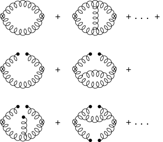
Figure 1: Diagrammatic representation of the OPE of the gluonic two-point correlator

$\bullet$ The $D=0$ operator corresponds to the usual case of the naïve perturbative contribution. In the massless light quark limit , some additionnal $D=2$ terms not included in the OPE may eventually manifest after the resummation of the QCD perturbative series [29]–[32]. However, due to the unclear present status of this contribution, and to the inaccurate quantitative control of the contribution of this term from ultraviolet renormalons calculus, we shall not explicitly consider this effect in our analysis. Alternatively, we estimate, like in the case of $\tau$ decay [33]–[35], the next unkown higher-order correction using a geometrical growth of the QCD series, which value is in agreement with the one from experimental measurements [36] and from an estimate [37] based on a $RS$-invariant approach within the principle of minimal sensitivity [38]. Then, we argue, like in the case of $\tau$ decay, that the errors induced by the truncation of the QCD series are given by this last term (theorem of divergent series [39]), which we have multiplied by a factor 2 as in [35] for a conservative estimate. The errors estimated in this way are comparable in strength with some of the previous UV renormalon estimates, and should already include in it this renormalon contribution (manifestation of the resummed QCD series). However, as mentioned previously, the UV renormalon estimate should be considered to be very qualitative at the present status of the art (dominance of the second chain of renormalons [32],…).
$\bullet$ The $D=4$ dimension operators, which will give the dominant contributions in the chiral limit $m_{i}=0$ is the gluonic condensate $\langle\alpha_{s}G^{2}\rangle$, introduced by SVZ [15], and which has been estimated recently from the $e^{+}e^{-}\rightarrow~{}I=1$ hadron data [40] and from the heavy quarks mass splittings [41]:

$$\langle\alpha_{s}G^{2}\rangle\simeq(0.07\pm 0.01)~{}\mbox{GeV}^{4},$$ (6)

in agreement with different post-SVZ estimates quoted in these papers.
$\bullet$ The $D=6$ contribution is dominated by the triple gluon condensate $gf_{abc}\langle G^{a}G^{b}G^{c}\rangle$, whose direct extraction from the data is still lacking. However, one can estimate its approximate value from the dilute gas instanton model [15]:

$$g^{3}f_{abc}\langle G^{a}G^{b}G^{c}\rangle\approx(1.5\pm 0.5)\mbox{GeV}^{2})\langle\alpha_{s}G^{2}\rangle~{},$$ (7)

where we have given the error in such a way that the estimate is valid within a factor 2.

$\bullet$ The validity of the SVZ expansion has been intensively studied in the theoretical literature [16], while the good agreement for the values of the QCD coupling $\alpha_{s}$ from $\tau$ decay [33]–[35] and LEP data , the observation of the running of $\alpha_{s}$ at low-scale [43], and the agreement of the measured QCD condensates from semi-inclusive tau decays and spectral moments [44] with the ones from phenomenological fits [40, 41], can be considered as its phenomenological confirmation.
$\bullet$ In the case of gluonia studied in this paper, it has also been argued [17], using the dilute gas approximation, that in some channels, instanton plus anti-instanton effects manifest themselves as higher dimension $(D=11)$ operators. On the other hand, its quantitative estimate is quite inaccurate because of the great sensitivity of the result on the QCD scale $\Lambda$, and on some other less controllable parameters and coefficients. However, at the scale (gluonia scale) where the following sum rules are optimized, which is much higher than the usual case of the $\rho$ meson, we consider that one can safely omit these terms like any other higher-dimensional operators beyond $D=8.$

3.2 The spectral function and its experimental measurement

The experimental measurement of the spectral function is best illustrated in the case of the flavour-diagonal light quark vector current, where the spectral function Im$\Pi$(t) can be related to the $e^{+}e^{-}$ into $I=1$ hadrons data via the optical theorem as:

$$\sigma(e^{+}e^{-}\rightarrow I=1~{}\mbox{hadrons})=\frac{4\pi^{2}\alpha}{t}e^{2}~{}\frac{1}{\pi}~{}\mbox{Im}\Pi(t).$$ (8)

One can also relate the spectral function to the leptonic width of the $\rho$ resonance:

$$\Gamma_{\rho\rightarrow e^{+}e^{-}}\simeq\frac{2}{3}\pi\alpha^{2}\frac{M_{\rho}}{2\gamma^{2}_{\rho}},$$ (9)

via the meson coupling to the electromagnetic current:

$$\langle 0|J^{\mu}|\rho\rangle=\frac{M^{2}_{\rho}}{2\gamma_{\rho}}\epsilon^{\mu},$$ (10)

within a vector meson dominance assumption. More generally, one can introduce the decay constant $f_{G}$ analogous to $f_{\pi}=93.3$ MeV:

$$\langle 0|J_{G}|G\rangle=\sqrt{2}f_{G}M_{G}^{2}~{}...,$$ (11)

where … represent the Lorentz structure of the matrix elements.

3.3 The form of the sum rules

On the phenomenological side, the improvement of the previous dispersion relation comes from the uses of an infinite number of derivatives and infinite values of $q^{2}$, but keeping their ratio fixed as $\tau\equiv n/q^{2}$. In this way, one obtains the Laplace or Borel or exponential sum rules [15, 45, 46]:

$${\cal L}_{G}(\tau)=\int_{t_{\leq}}^{\infty}{dt}~{}\mbox{exp}(-t\tau)~{}\frac{1}{\pi}~{}\mbox{Im}\psi_{G}(t),$$ (12)

where $t_{\leq}$ is the hadronic threshold. The advantage of this sum rule with respect to the previous dispersion relation is the presence of the exponential weight factor, which enhances the contribution of the lowest resonance and low-energy region accessible experimentally. For the QCD side, this procedure has eliminated the ambiguity carried by subtraction constants, arbitrary polynomial in $q^{2}$, and has improved the convergence of the OPE by the presence of the factorial dumping factor for each condensates of given dimensions.

The ratio of sum rules:

$${\cal R}_{G}\equiv-\frac{d}{d\tau}\log{{\cal L}_{G}},$$ (13)

or its slight modification, is a useful quantity to work with, in the determination of the resonance mass, as it is equal to the mass squared, in the simple duality ansatz parametrization:

$$``\mbox{one resonance}"\delta(t-M^{2}_{R})\ +\ ``\mbox{QCD continuum}"\Theta(t-t_{c}),$$ (14)

of the spectral function, where the resonance enters by its coupling to the quark current; $t_{c}$ is the continuum threshold which is, like the sum rule variable $\tau$, an a priori arbitrary parameter. As tested in the meson channels, this parametrization gives a good description of the spectral integral, in the sum rule analysis. In some cases, we shall also use finite energy sum Rule (FESR) [47, 19]:

$${\cal M}_{G}^{(n)}=\int_{t_{\leq}}^{t_{c}}{dt}~{}t^{n}~{}\frac{1}{\pi}~{}\mbox{Im}\psi_{G}(t),~{}~{}~{}~{}~{}~{}~{}~{}~{}~{}{\cal R}_{G}^{(n)}\equiv\frac{{\cal M}_{G}^{(n)}}{{\cal M}_{G}^{(n+1)}},$$ (15)

where $n$ is an integer, in order to double check the estimate obtained from the Laplace sum rules.

3.4 Conservative optimization criteria

Different optimization criteria are proposed in the literature, which, to my opinion, complete one another, if used carefully. The sum rule window of SVZ is a compromise region where, at the same time, the OPE makes sense while the spectral integral is still dominated by the lowest resonance. This is indeed satisfied when the Laplace sum rule presents a minimum in $\tau$, where there is an equilibrium between the non-perturbative and high-energy region effects. However, this criterion is not yet sufficient as the value of this minimum in $\tau$ can still be greatly affected by the value of the continuum threshold $t_{c}$. The needed extra condition is to find the region where the result has also a minimal sensitivity on the change of the $t_{c}$ values ($t_{c}$ stability). The $t_{c}$ values obtained in this way are about the same as the one from the so-called heat evolution test of the local duality FESR [47]. However, in some cases, this $t_{c}$ value is too high, compared with the mass of the observed radial excitation, and the procedure tends to overestimate the predictions. More precisely, the result obtained in this way can be considered as a phenomenological upper limit. Therefore, in order to have a conservative prediction from the sum rules method, one can consider the value of $t_{c}$ at which one starts to have a $\tau$-stability up to where one has a $t_{c}$ stability. In case there is no $t_{c}$ stability nor FESR constraint on $t_{c}$, one can consider that the prediction is still unreliable. In this paper, we shall limit ourselves to extracting the results satisfying the $\tau$ (Laplace) or $n$ (FESR) and $t_{c}$ stability criteria.

4 Mass and decay constant of the $0^{++}$ scalar gluonia

4.1 The gluonium two-point correlator in QCD

We shall be concerned with the correlator:

$$\psi_{s}(q^{2})\equiv 16i\int d^{4}x~{}e^{iqx}~{}\langle 0|{\cal T}\theta^{\mu}_{\mu}(x)\theta^{\mu}_{\mu}(0)^{\dagger}|0\rangle,$$ (16)

where $\theta_{\mu\nu}$ is the improved QCD energy-momentum tensor (neglecting heavy quarks) whose anomalous trace reads, in standard notations:

$$\theta^{\mu}_{\mu}(x) = \frac{1}{4}\beta(\alpha_{s})G^{2}+(1+\gamma_{m}(\alpha_{s}))\sum_{u,d,s}m_{i}\bar{\psi}_{i}\psi_{i}.$$ (17)

Its leading-order perturbative and non-perturbative expressions in $\alpha_{s}$ have been obtained by the authors of [17]. To two-loop accuracy in the $\overline{MS}$ scheme, its perturbative expression has been obtained by [48], while the radiative correction to the gluon condensate has been derived in [23]. Using a simplified version of the notation in Eq. (5):

$$\psi_{s}(q^{2})=\sum_{D=0,4,...}C_{D}\langle O_{D}\rangle,$$ (18)

one obtains for three flavours and by normalizing the result with $(\beta(\alpha_{s})/\alpha_{s})^{2}$:

$$C_{0} = -2\left(\frac{{\alpha_{s}}}{\pi}\right)^{2}(-q^{2})^{2}\log{-\frac{q^{2}}{\nu^{2}}}\left\{1+\frac{59}{4}\left(\frac{{\alpha_{s}}}{\pi}\right)+\frac{\beta_{1}}{2}\left(\frac{{\alpha_{s}}}{\pi}\right)\log{-\frac{q^{2}}{\nu^{2}}}\right\}$$

$$C_{4}\langle O_{4}\rangle = 4\alpha_{s}\left\{1+\frac{49}{12}\left(\frac{{\alpha_{s}}}{\pi}\right)+\frac{\beta_{1}}{2}\left(\frac{{\alpha_{s}}}{\pi}\right)\log{-\frac{q^{2}}{\nu^{2}}}\right\}\langle\alpha_{s}G^{2}\rangle$$

$$C_{6}\langle O_{6}\rangle = 2\left(\frac{\bar{\alpha_{s}}}{\pi}\right)\left\{1-\frac{29}{4}\alpha_{s}\log{-\frac{q^{2}}{\nu^{2}}}\right\}g^{3}f_{abc}\langle G^{a}G^{b}G^{c}\rangle$$

$$C_{8}\langle O_{8}\rangle = 14\langle\left(\alpha_{s}f_{abc}G^{a}_{\mu\rho}G^{b\rho}_{\nu}\right)^{2}\rangle-\langle\left(\alpha_{s}f_{abc}G^{a}_{\mu\nu}G^{b}_{\rho\lambda}\right)^{2}\rangle.$$ (19)

From its asymptotic behaviour ($q^{4}\log$), we can write a twice-subtracted dispersion relation for $\psi_{s}(q^{2})$:

$$\psi_{s}(q^{2})=\psi_{s}(0)+q^{2}\psi^{\prime}_{s}(0)+q^{4}\int_{0}^{\infty}\frac{dt}{t^{2}(t-q^{2}-i\epsilon)}\frac{1}{\pi}\mbox{Im}\psi_{s}(t),$$ (20)

where the subtraction constant $\psi_{s}(0)$ is known from the LET to be [17]:

$$\psi_{s}(0)=-16\frac{\beta_{1}}{\pi}\langle\alpha_{s}G^{2}\rangle.$$ (21)

4.2 The gluonium sum rules

Using standard QSSR technology, one can derive, from the previous expression of the two-point correlator, the unsubtracted Laplace sum rule (USR):

$${\cal L}_{s}^{(0)} \equiv \int_{t_{\leq}}^{\infty}{dt}~{}\mbox{exp}(-t\tau)~{}\frac{1}{\pi}~{}\mbox{Im}\psi_{s}(t)$$

$$= \frac{4}{\pi^{2}}\beta^{2}(\alpha_{s})\tau^{-3}\Bigg{[}\Bigg{[}1+\frac{1}{4}\left(\frac{\bar{\alpha_{s}}}{\pi}\right)\left(59+2\beta_{1}(1-2\gamma_{E})-4\frac{\beta_{2}}{\beta_{1}}\log{-\log({\tau\Lambda^{2})}}\right)\Bigg{]}$$

$$-\pi\frac{\beta_{1}}{2}\langle\alpha_{s}G^{2}\rangle\tau^{2}+\frac{\pi}{2\alpha_{s}}g^{3}f_{abc}\langle G^{a}G^{b}G^{c}\rangle\tau^{3}+\frac{2\pi^{3}}{\alpha_{s}}\langle\alpha_{s}G^{2}\rangle^{2}\tau^{4}\Bigg{]}$$

$${\cal L}_{s}^{(1)} \equiv -\frac{d}{d\tau}{\cal L}_{s}^{(0)},$$

$${\cal L}_{s}^{(2)} \equiv -\frac{d}{d\tau}{\cal L}_{s}^{(1)}$$ (22)

and the subtracted sum rule (SSR), which depends crucially on the subtraction constant $\psi_{s}(0)$:

$${\cal L}_{s}^{(-1)} \equiv \int_{t_{\leq}}^{\infty}\frac{dt}{t}~{}\mbox{exp}(-t\tau)~{}\frac{1}{\pi}~{}\mbox{Im}\psi_{s}(t)$$ (23)

$$= \frac{2}{\pi^{2}}\beta^{2}(\alpha_{s})\tau^{-2}\Bigg{[}1+\frac{1}{4}\left(\frac{\bar{\alpha_{s}}}{\pi}\right)\left(59+4\beta_{1}(1-\gamma_{E})-4\frac{\beta_{2}}{\beta_{1}}\log{-\log{(\tau\Lambda^{2})}}\right)\Bigg{]}$$

$$+\psi_{s}(0)-{4}\frac{\beta^{2}(\alpha_{s})}{\alpha_{s}}\Bigg{[}\langle\alpha_{s}G^{2}\rangle\Bigg{[}1+\left(\frac{\bar{\alpha_{s}}}{\pi}\right)\left(\frac{49}{12}-\frac{\gamma_{E}}{2}\beta_{1}\right)\Bigg{]}$$

$$+\frac{\tau}{2\pi}g^{3}f_{abc}\langle G^{a}G^{b}G^{c}\rangle+\pi\langle\alpha_{s}G^{2}\rangle^{2}\tau^{2}\Bigg{]},$$

where:

$$\left(\frac{\bar{\alpha_{s}}}{\pi}\right)\equiv\frac{1}{\beta_{1}\log{\sqrt{\tau}\Lambda}}.$$ (24)

Throught this paper, we shall use for three active flavours [42]:

$$\Lambda=(375\pm 125)~{}\mbox{MeV}.$$ (25)

$\bullet$ One can notice that the perturbative correction is large for the Laplace sum rules ${\cal L}_{s}^{(n)}$, but it tends to cancel in the ratio of moments. As discussed earlier, we estimate the higher-order unknown perturbative corrections using a geometrical growth of the QCD series. Then, we expect that the “effective” $\alpha_{s}^{2}$ correction including $\log\log$ terms normalized to the lowest-order perturbative graph is here about:

$$\delta_{\alpha}^{(4)}\approx\pm 2\times 18\left(\frac{\bar{\alpha_{s}}}{\pi}\right)^{2}~{},$$ (26)

which we consider as the error due to the truncation of the perturbative QCD series (last known term of the series), which should include in it some (eventual) effects of the 1/$Q^{2}$-term induced by the resuumation of this series. The factor 2 is a conservative estimate of the errors.
$\bullet$ We shall see later on, that the non-perturbative contributions including the corresponding $\alpha_{s}$ corrections are small at the scale where the sum rules are optimized, such that the dominant errors from the non-perturbative effects come from the values of the condensates.
$\bullet$ One should also notice that it can be inconsistent to work here in a pure Yang-Mills, as our QCD parameters ($\alpha_{s}$ and gluon condensates) have been extracted from the data in the presence of quarks. Therefore, one should be careful in comparing the results in the present paper with e.g. the lattice ones.
$\bullet$ The USR ${\cal L}_{s}^{(0)}$ and the SSR ${\cal L}_{s}^{(-1)}$ have been used in NV. The authors of Ref. [17] have also used the SSR in order to set the sum rule scale in the scalar gluonium channel, leading to the conclusion that the scalar gluonium energy scale should be much larger (or $\tau$ much smaller) than the one of ordinary hadrons. We shall see later on that the SSR ${\cal L}_{s}^{(-1)}$ satisfies this criteria, due mainly to the relative importance of the $\psi_{s}(0)$ contribution. However, this conclusion is not universal, as it does not necessarily apply to the USR, where $\tau$ can be slightly larger (or the sum rule energy scale slightly lower) than in the SSR. A simple inspection of these different sum rules indicates that ${\cal L}_{s}^{(0)}$ is the only sum rule that can be sensitive to a low-mass resonance below 1 GeV, as it is a low moment in $t$ and it can stabilize at large value of $\tau$. Higher moments in $t$, ${\cal L}_{s}^{(1,2)}$,are, on the contrary, sensitive to a higher mass resonance. As discussed before, ${\cal L}_{s}^{(-1)}$ is quite particular since, though it is the lowest moment, which a priori can be more sensitive to the lowest meson mass, its stability is pushed to higher energies because of the relatively large value of $\psi_{s}(0)$. As a biproduct, ${\cal L}_{s}^{(-1)}$ becomes less sensitive to a low-mass resonance than ${\cal L}_{s}^{(0)}$.

4.3 Mass of the gluonium $G$

In order to study the properties of the gluonium $G$ expected from other approaches to be in the range of 1.4 to 2 GeV, we have to work with sum rules that are more sensitive to the high-energy region than ${\cal L}_{s}^{(0)}$. Using the positivity of the spectral functions, an upper bound on the gluonium mass squared can be obtained from the minimum (or inflexion point) of the ratios :

$${\cal R}_{21}\equiv\frac{{\cal L}_{s}^{(2)}}{{\cal L}_{s}^{(1)}},$$ (27)

giving (see Fig. 2):

$$M_{G}\leq(2.16\pm 0.16\pm 0.14\pm 0.05)~{}\mbox{GeV},$$ (28)

where the errors come respectively from the value of $\Lambda$, from the estimated unknown higher-order terms and from the gluon condensate. At such a small value of $\tau$, where the sum rule is optimized, we expect that high-dimension terms including instanton effects are highly suppressed. Combining these errors in quadrature, we obtain:

$$M_{G}\leq(2.16\pm 0.22)~{}\mbox{GeV},$$ (29)

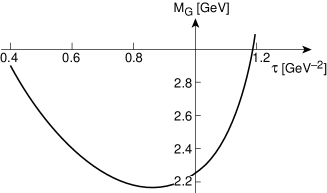
Figure 2: $\tau$ behaviour of the ratio of moments ${\cal R}^{1/2}_{21}$. Its minimum corresponds to an upper bound for the scalar gluonium mass.

An estimate of the mass squared can be obtained using the duality ansatz parametrization of the spectral functions, which leads to the FESR-like ratios

$${\cal R}_{21}^{c}\equiv\frac{\int_{t_{\leq}}^{t_{c}}{dt~{}}{t^{2}}~{}\mbox{exp}(-t\tau)~{}\frac{1}{\pi}~{}\mbox{Im}\psi_{G}(t)~{}}{\int_{t_{\leq}}^{t_{c}}{dt}~{}t~{}\mbox{exp}(-t\tau)~{}\frac{1}{\pi}~{}\mbox{Im}\psi_{G}(t)}\simeq M^{2}_{G},$$ (30)

where $t_{c}$ is the QCD continuum threshold. Neglecting in the analysis the eventual contribution of the light $\sigma_{B}$ of a mass below 1 GeV, which is justified by the higher power of mass suppression in the present sum rule, we show in Fig. 3a, b the stabilities in $\tau$ (here it is an inflexion point) and in $t_{c}$ (here it is a minimum) of the estimate.

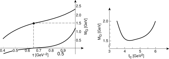
Figure 3: a): $\tau$ behaviour of the estimated value of the scalar gluonium mass for $t_{c}=4.5$ GeV². The optimal value is at the inflexion point corresponding to the zero of its second derivative in $\tau$. b): $t_{c}$ behaviour of $M_{G}$.

Then, we deduce the optimal result:

$$M_{G}\simeq(1.50\pm 0.10\pm 0.15\pm 0.05)~{}\mbox{GeV},$$ (31)

where the errors are due to $\Lambda$, the estimated unknown higher-order terms and the gluon condensate. Combining these errors in quadrature, we obtain:

$$M_{G}\simeq(1.50\pm 0.19)~{}\mbox{GeV},$$ (32)

in agreement with the most recent sum rule result in [23]. Within the sum rule approach, one can approximately identify the value of $t_{c}$ as the mass squared of the next radial excitation:

$$M_{G^{\prime}}\approx\sqrt{t_{c}}\simeq(2.0\sim 2.1)~{}\mbox{GeV},$$ (33)

where it can be noticed that, unlike the usual hadrons, the splitting between the lowest ground states and the radial excitations are relatively small ($\Delta M_{G}/M_{G}\approx 30\%$ compared with $\Delta M_{\rho}/M_{\rho}\geq 70\%$). One can compare our value of $M_{G}$ with the theoretical estimates (lattice calculations [9]–[11], QCD inequalities [12], …) and with the GAMS [7] and Crystal Barrel [14] data.

4.4 Decay constant of the G(1.5)

The decay constant of the G(1.5) can be introduced via:

$$\langle 0|4\theta^{\mu}_{\mu}|G\rangle=\sqrt{2}f_{G}M^{2}_{G},$$ (34)

where $f_{G}$ is the decay constant analogue of $f_{\pi}$. One can either estimate $f_{G}$, by using the previous ${\cal L}^{(1,2)}_{s}$ sum rules, or using the SSR ${\cal L}_{s}^{(-1)}$, as in NV, which we shall discuss later on. Using the previous sum rules, for instance ${\cal L}^{(1)}_{s}$, we obtain (see Fig. 4):

$$f_{G}\simeq(390\pm 98\pm 65\pm 39\pm 76)~{}\mbox{MeV},$$ (35)

where the errors come from $\Lambda$, the estimated unknown higher-order terms, the gluon condensate and the value of $t_{c}$. Combining these errors in quadrature, we obtain:

$$f_{G}\simeq(390\pm 145)~{}\mbox{MeV},$$ (36)

which we shall use later on. However, one should remark that the errors in the present determinations are relatively large compared with the typical 10-20$\%$ accuracy in the QSSR estimate of the corresponding quantity in the ordinary hadron sector.

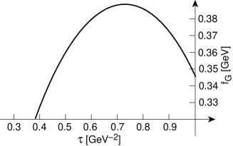
Figure 4: $\tau$-behaviour of the decay constant $f_{G}$ from ${\cal L}^{(1)}_{s}$.

4.5 Mass and decay constant of the three-gluon bound state

Recall that a QSSR analysis of the two-point correlator associated to the scalar three-gluon local current to leading order [24, 16]:

$$J_{3G}=g^{3}f_{abc}G^{a}G^{b}G^{c}$$ (37)

leads to the mass prediction:

$$M_{3G}\simeq 3.1~{}\mbox{GeV}~{}~{}~{}~{}~{}~{}~{}~{}\sqrt{t_{c}}\simeq 3.4~{}\mbox{GeV},$$ (38)

and to the value of the decay constant of:

$$f_{3G}\simeq 62~{}\mbox{MeV},$$ (39)

which is relatively high compared with the mass of the gluonium built from the two-gluon current, and which makes the mass-mixing between these two gluonia states tiny [24, 16]:

$$\theta_{3}\approx 4^{\circ}~{},$$ (40)

where the accuracy for the above predictions are about 10-20$\%$. This state might be produced in the radiative decay of heavy quarkonia, when phase space permits, while its experimental search can be done by measuring some typical gluonia decays into the pairs $\eta^{\prime}\eta^{\prime}$ or $\eta\eta^{\prime}$.

4.6 Decay constants of the $\sigma_{B}$ and $\sigma^{\prime}_{B}$ mesons

As discussed previously and in NV, one can expect that the low moments ${\cal L}_{s}^{(-1,0)}$ are sensitive to the low-mass resonances whose effects can have been missed in the previous analysis of ${\cal L}_{s}^{(1,2)}$, and presumably in the lattice calculations within a one-resonance parametrization. In the following, we shall therefore test the “gluonium” nature of the broad low-mass states $\sigma_{B}$ and $\sigma^{\prime}_{B}$, where the former, which has a mass in the range 0.5 to 1 GeV, is the one seen in $\gamma\gamma$ and $\pi\pi$ scattering experiments, and expected from the linear $\sigma$ model [8, 49], while we identify the second as its radial excitation with a mass close to that of the observed state at 1.37 GeV. We use a three-resonance ($\sigma_{B}$, $\sigma^{\prime}_{B}$ and $G(1.5)$) parametrization of the spectral function . We introduce the previous values of the $G(1.5)$ parameters and the corresponding value of $t_{c}\simeq 4.5$ GeV². Using as input $M_{\sigma^{\prime}_{B}}\approx 1.37$ GeV and $M_{\sigma_{B}}\approx(0.5\sim 1)$ GeV, we extract from the two sum rules the decay constants of the $\sigma_{B}$ and $\sigma^{\prime}_{B}$ within the $\tau$-stability criteria. We show in Fig. 5 the $\tau$ behaviour of:

$$\tilde{f}_{2}\equiv f_{\sigma_{B}}\left(1+\rho~{}\exp{(M^{2}_{\sigma^{\prime}_{B}}-M^{2}_{\sigma_{B}})\tau}\right)^{1/2},$$ (41)

and of:

$$\tilde{f}_{4}\equiv f_{\sigma_{B}}\left(1+\rho\frac{M^{2}_{\sigma^{\prime}_{B}}}{M^{2}_{\sigma_{B}}}~{}\exp{(M^{2}_{\sigma^{\prime}_{B}}-M^{2}_{\sigma_{B}})\tau}\right)^{1/2},$$ (42)

where:

$$\rho\equiv\frac{M^{2}_{\sigma^{\prime}_{B}}f_{\sigma^{\prime}_{B}}}{M^{2}_{\sigma_{B}}f_{\sigma_{B}}}.$$ (43)

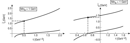
Figure 5: $\tau$ behaviour of the decay constants $\tilde{f}_{2}$ from ${\cal L}^{(-1)}_{s}$ and $\tilde{f}_{4}$ from ${\cal L}^{(0)}_{s}$

Then, we deduce:

$$f_{\sigma_{B}}[\mbox{GeV}]\approx 1.0~{}~{}~{}~{}~{}~{}~{}~{}~{}~{}f_{\sigma^{\prime}_{B}}[\mbox{GeV}]\approx 0.6~{}~{}~{}~{}~{}\mbox{for}~{}~{}~{}~{}M_{\sigma_{B}}[\mbox{GeV}]\approx 1.0$$ (44)

$$1.4~{}~{}~{}~{}~{}~{}~{}~{}~{}~{}~{}~{}~{}~{}~{}~{}~{}~{}~{}~{}~{}~{}~{}~{}~{}~{}~{}0.7~{}~{}~{}~{}~{}~{}~{}~{}~{}~{}~{}~{}~{}~{}~{}~{}~{}~{}~{}~{}~{}~{}~{}~{}~{}~{}~{}~{}~{}~{}~{}0.75$$

$$1.9~{}~{}~{}~{}~{}~{}~{}~{}~{}~{}~{}~{}~{}~{}~{}~{}~{}~{}~{}~{}~{}~{}~{}~{}~{}~{}~{}0.5~{}~{}~{}~{}~{}~{}~{}~{}~{}~{}~{}~{}~{}~{}~{}~{}~{}~{}~{}~{}~{}~{}~{}~{}~{}~{}~{}~{}~{}~{}~{}0.5~{},$$

which indicates the necessity to have “low-mass gluonia” (which, as we shall see later on, couples strongly to $\pi\pi$) for the consistency of the sum rules approach , although their effects are negligible in the high-moments analysis. The previous quantities will be useful later on for studying the $\sigma_{B}$ and $\sigma^{\prime}_{B}$ decays.

5 Decay widths of the $\sigma_{B}$, $\sigma^{\prime}_{B}$ and $G$

5.1 $\sigma_{B}$ and $\sigma^{\prime}_{B}$ couplings to $\pi\pi$

At this point, we use vertex sum rules to obtain further constraints. We consider the vertex (Fig. 6a):

$$V(q^{2})=\langle\pi_{1}|\theta^{\mu}_{\mu}|\pi_{2}\rangle,~{}~{}~{}~{}~{}q=p_{1}-p_{2}~{},$$ (45)

where:

$$V(0)=2m^{2}_{\pi}~{}.$$ (46)

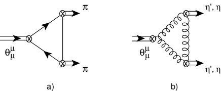
Figure 6: Vertex controlling the gluonium couplings to: a) $\pi\pi$; b) $\eta(\eta^{\prime})-\eta(\eta^{\prime})$.

In the chiral limit $(m^{2}_{\pi}\simeq 0)$, the vertex obeys the dispersion relation:

$$V(q^{2})=\int_{0}^{\infty}\frac{dt}{t-q^{2}-i\epsilon}~{}\frac{1}{\pi}\mbox{Im}V(t),$$ (47)

which gives, by saturating with the three resonances $\sigma_{B}$, $\sigma^{\prime}_{B}$ and $G$:

$$\frac{1}{4}\sum_{S=\sigma_{B},\sigma^{\prime}_{B},G}g_{S\pi\pi}\sqrt{2}f_{S}\simeq 0.$$ (48)

Using the fact that $V^{\prime}(0)=1$ [51] from a generalization of the Goldberger-Treiman relation using soft-pion techniques, one obtains a second sum rule:

$$\frac{1}{4}\sum_{i=\sigma_{B},\sigma^{\prime}_{B},G}g_{S\pi\pi}\sqrt{2}f_{S}/M^{2}_{S}=1.$$ (49)

Identifying the $G$ with the $G(1.5\sim 1.6)$ at GAMS and the Crystal Barrel, we can neglect then its coupling to $\pi\pi$. Therefore, we can deduce:

$$g_{\sigma_{B}\pi\pi} \approx \frac{4}{\sqrt{2}f_{\sigma_{B}}}~{}\frac{1}{\left(1-M^{2}_{\sigma_{B}}/M^{2}_{\sigma^{\prime}_{B}}\right)}$$

$$g_{\sigma^{\prime}_{B}\pi\pi} \approx g_{\sigma_{B}\pi\pi}\left(\frac{f_{\sigma_{B}}}{f_{\sigma^{\prime}_{B}}}\right),$$ (50)

Fixing for definiteness $M_{\sigma^{\prime}_{B}}\simeq 1.37$ GeV, one can deduce the width into $\pi\pi~{}(\pi^{+}\pi^{-},~{}2\pi^{0})$:

$$\Gamma(\sigma_{B}\rightarrow\pi\pi)[\mbox{GeV}] \approx 0.7~{}~{}~{}~{}~{}~{}~{}~{}~{}~{}\Gamma(\sigma^{\prime}_{B}\rightarrow\pi\pi)[\mbox{GeV}]\approx~{}~{}1.3~{}~{}~{}~{}~{}\mbox{for}~{}~{}~{}~{}M_{\sigma_{B}}[\mbox{GeV}]\approx 1.0$$ (51)

$$0.2~{}~{}~{}~{}~{}~{}~{}~{}~{}~{}~{}~{}~{}~{}~{}~{}~{}~{}~{}~{}~{}~{}~{}~{}~{}~{}~{}~{}~{}~{}~{}~{}~{}~{}~{}~{}~{}~{}~{}~{}0.5~{}~{}~{}~{}~{}~{}~{}~{}~{}~{}~{}~{}~{}~{}~{}~{}~{}~{}~{}~{}~{}~{}~{}~{}~{}~{}~{}~{}~{}~{}~{}0.75$$

$$0.1~{}~{}~{}~{}~{}~{}~{}~{}~{}~{}~{}~{}~{}~{}~{}~{}~{}~{}~{}~{}~{}~{}~{}~{}~{}~{}~{}~{}~{}~{}~{}~{}~{}~{}~{}~{}~{}~{}~{}~{}0.9~{}~{}~{}~{}~{}~{}~{}~{}~{}~{}~{}~{}~{}~{}~{}~{}~{}~{}~{}~{}~{}~{}~{}~{}~{}~{}~{}~{}~{}~{}~{}0.5~{},$$

where

$$\Gamma(\sigma_{B}\rightarrow\pi\pi)=\frac{|g_{\sigma_{B}\pi\pi}|^{2}}{16\pi M_{\sigma_{B}}}\left({1-\frac{4m^{2}_{\pi}}{M^{2}_{\sigma_{B}}}}\right)^{1/2}.$$ (52)

We have repeated the derivation of $f_{\sigma_{B}}$ by taking into account finite-width corrections. This leads to an increase of $f_{\sigma_{B}}$, which is compensated by the propagator effect in the estimate of $g_{\sigma_{B}\pi\pi}$, i.e. the result obtained from the vertex sum rule remains almost unchanged. It is interesting to see from the sum rule that a very light $\sigma_{B}$ around $500$ MeV cannot be broad, which seems not to be favoured by the present data. Improvements of the data analysis are required for refining the mass measurement of the $\sigma_{B}$. Our result indicates the presence of gluons inside the wave functions of the broad resonance below 1 GeV and the $\sigma^{\prime}(1.37)$, which can decay copiously into $\pi\pi$ .

5.2 G(1.5) coupling to $\eta$$\eta^{\prime}$

In order to compute these couplings, we consider the three-point function (Fig. 6b):

$$\tilde{V}_{\mu\nu}(q_{1},q_{2})\equiv\int d^{4}x_{1}~{}d^{4}x_{2}~{}e^{i(q_{1}x_{1}+q_{2}x_{2})}~{}\langle 0|{\cal T}Q(x_{1})Q(x_{2})\theta_{\mu\nu}(0)|0\rangle~{},$$ (53)

where $\theta_{\mu\nu}$ is the energy momentum tensor of QCD with three light quarks, while $Q(x)$ is the topological charge density defined previously. Using the low-energy theorem:

$$\langle\eta_{1}|\theta^{\mu}_{\mu}|\eta_{1}\rangle=2M^{2}_{\eta_{1}},$$ (54)

where $\eta_{1}$ is the unmixed $U(1)$ singlet state of mass $M_{\eta_{1}}\simeq$ 0.76 GeV [52], and writing the dispersion relation for the vertex, one obtains the NV sum rule:

$$\frac{1}{4}\sum_{S\equiv\sigma_{B},\sigma^{\prime}_{B},G}g_{S\eta_{1}\eta_{1}}\sqrt{2}f_{S}=2M^{2}_{\eta_{1}},$$ (55)

which implies, for $M_{\sigma_{B}}\simeq(0.75\sim 1)$ GeV, and by assuming a $G$-dominance of the vertex sum rule:

$$g_{G\eta_{1}\eta_{1}}\approx(1.2\sim 1.7)~{}\mbox{GeV}.$$ (56)

Introducing the “physical” $\eta^{\prime}$ and $\eta$ through:

$$\eta^{\prime}\sim\cos\theta_{P}\eta_{1}-\sin\theta_{P}\eta_{8}$$

$$\eta\sim\sin\theta_{P}\eta_{1}+\cos\theta_{P}\eta_{8},$$ (57)

where [53, 54]

$$\theta_{P}\simeq-(18\pm 2)^{\circ}$$ (58)

is the pseudoscalar mixing angle, one obtains:

$$\Gamma(G\rightarrow\eta\eta^{\prime})\simeq(5\sim 10)~{}\mbox{MeV}.$$ (59)

The previous scheme is also known to predict (see NV and [6]):

$$r\equiv\Gamma_{G\eta\eta}/\Gamma_{G\eta\eta^{\prime}}\simeq 0.22,~{}~{}~{}~{}~{}~{}~{}~{}~{}~{}~{}~{}g_{G\eta\eta}\simeq\sin\theta_{P}g_{G\eta\eta^{\prime}}~{}~{}~{}\Longrightarrow\Gamma_{G\eta\eta}\simeq(1.1\sim 2.2)~{}\mbox{MeV}.$$ (60)

compared with the GAMS data [7] $r\simeq 0.34\pm 0.13$. This result, can then suggest that the $G(1.6)$ seen by the GAMS group is a pure gluonium, which is not the case of the particle seen by Crystal Barrel [14].

5.3 $\sigma^{\prime}_{B}(1.37)$ and G(1.5) couplings to $4\pi$ through $\sigma_{B}\sigma_{B}$

Within our scheme, we expect that the $4\pi$ are mainly initiated from the decay of pairs of $\sigma_{B}$. A LET analogous to that in previous cases, can be written for the estimate of $g_{G\sigma_{B}\sigma_{B}}$. Using

$$\langle\sigma_{B}|\theta^{\mu}_{\mu}|\sigma_{B}\rangle=2M^{2}_{\sigma_{B}}$$ (61)

and writing the dispersion relation for the vertex, one obtains the sum rule:

$$\frac{1}{4}\sum_{i=\sigma_{B},\sigma^{\prime}_{B},G}g_{S\sigma_{B}\sigma_{B}}\sqrt{2}f_{S}=2M^{2}_{\sigma_{B}}.$$ (62)

We identify the $\sigma^{\prime}_{B}$ with the observed $f_{0}(1.37)$. Using the observed value of the width into $4\pi$ [53, 55] and extracting the $S$-wave part, which we assume to be initiated from $2\sigma_{B}$, we deduce :

$$\Gamma(\sigma^{\prime}_{B}\rightarrow(4\pi)_{S})\simeq(46\sim 316)~{}\mbox{MeV}~{}\Longrightarrow~{}g_{\sigma^{\prime}_{B}\sigma_{B}\sigma_{B}}\simeq(2.3\sim 5.9)~{}\mbox{GeV},$$ (63)

where we have taken finite width corrections from the Breit-Wigner parametrization of the $\sigma_{B}$ resonance. We have used $M_{\sigma_{B}}\simeq 1$ GeV and $\Gamma(\sigma_{B}\rightarrow\pi\pi)\simeq 0.7$ GeV. Neglecting, to a first approximation, the $\sigma_{B}$ contribution to the sum rule, we can deduce:

$$g_{G\sigma_{B}\sigma_{B}}\approx(2.7\sim 4.3)~{}\mbox{GeV},$$ (64)

which, despite the large error, is larger than the $G\eta_{1}\eta_{1}$ coupling. It can indicate that the decay of a pure gluonium state can be dominated (phase space permitting) by the $4\pi$ branching ratio initiated from the pair of $\sigma$-mesons, as already emphasized by NV. Using the previous values and the corresponding decay constant and width, one can deduce, using a Breit-Wigner form:

$$\Gamma(G\rightarrow\sigma_{B}\sigma_{B}\rightarrow 4\pi)\simeq(60\sim 138)~{}\mbox{MeV}.$$ (65)

This feature seems to be satisfied by the states seen by GAMS and the Crystal Barrel. Our approach shows the consistency in interpreting the $G(1.6)$ seen at GAMS as an “almost” pure gluonium state (ratio of the $\eta\eta^{\prime}$ versus the $\eta\eta$ widths), while the state seen by the Crystal Barrel, though having a gluon component in its wave function, cannot be a pure gluonium because of its prominent decays into $\eta\eta$ and $\pi^{+}\pi^{-}$. We shall see later on that the Crystal Barrel state can be better explained from a quarkonium-gluonium mixing.

5.4 $\sigma_{B}$, $\sigma^{\prime}_{B}$ and $G$ couplings to $\gamma\gamma$

The two-photon widths of the $\sigma,~{}\sigma^{\prime}$ and $G$ can be obtained by identifying the Euler-Heisenberg effective Lagrangian (Fig. 7a) [51]:

$${\cal L}_{\gamma g} = \frac{\alpha\alpha_{s}Q^{2}_{q}}{180m^{2}_{q}}[28F_{\mu\nu}F_{\nu\lambda}G_{\lambda\sigma}G_{\sigma\mu}+14F_{\mu\nu}G_{\nu\lambda}F_{\lambda\sigma}G_{\sigma\mu}$$ (66)

$$- F_{\mu\nu}G_{\mu\nu}F_{\alpha\beta}G_{\alpha\beta}-F_{\mu\nu}F_{\mu\nu}G_{\alpha\beta}G_{\alpha\beta}],$$

where $Q_{q}$ is the quark charge in units of $e$, $-\beta_{1}=9/2$ for three flavours, and $m_{q}$ is the “constituent” quark mass, which we shall take to be

$$m_{u}\simeq m_{d}\simeq M_{\rho}/2,~{}~{}~{}~{}~{}~{}~{}~{}m_{s}\simeq M_{\Phi}/2~{},$$ (67)

with the scalar-$\gamma\gamma$ Lagrangian

$${\cal L}_{S\gamma\gamma}=g_{S\gamma\gamma}\sigma_{B}(x)F^{(1)}_{\mu\nu}F^{(2)}_{\mu\nu}.$$ (68)

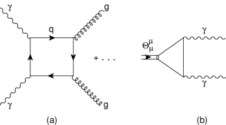
Figure 7: Vertex controlling the gluonium couplings to $J/\psi(\gamma)\gamma$: a) box diagram; b) anomaly diagram.

This leads to the sum rule:

$${g_{S\gamma\gamma}}\simeq\frac{\alpha}{60}\sqrt{2}{f_{\sigma_{B}}M^{2}_{\sigma_{B}}}\left(\frac{\pi}{-\beta_{1}}\right)\sum_{q\equiv u,d,s}{Q^{2}_{q}/m_{q}^{4}},$$ (69)

from which we deduce the couplings :

$$g_{\sigma_{B}\gamma\gamma}\approx(0.4\sim 0.7)\alpha~{}\mbox{GeV}^{-1}~{}~{}~{}~{}~{}~{}~{}~{}~{}~{}~{}~{}~{}~{}~{}~{}~{}~{}~{}g_{\sigma^{\prime}_{B}\gamma\gamma}\approx(0.5\sim 0.6)\alpha~{}\mbox{GeV}^{-1}~{}~{}~{}~{}~{}~{}~{}~{}~{}~{}~{}~{}~{}~{}~{}~{}~{}~{}~{}g_{G\gamma\gamma}\approx(0.6\pm 0.2)\alpha~{}\mbox{GeV}^{-1}.$$ (70)

Using the corresponding decay width:

$$\Gamma(S\rightarrow\gamma\gamma)=\frac{|g_{S\gamma\gamma}|^{2}}{16\pi}M^{3}_{S},$$ (71)

one obtains:

$$\Gamma(\sigma_{B}\rightarrow\gamma\gamma)\approx(0.2\sim 0.3)~{}\mbox{ keV}~{}~{}~{}~{}~{}~{}~{}\Gamma(\sigma^{\prime}_{B}\rightarrow\gamma\gamma)\approx(0.7\sim 1.0)~{}\mbox{ keV}~{}~{}~{}~{}~{}~{}~{}\Gamma(G\rightarrow\gamma\gamma)\approx(1.0\pm 0.8)~{}\mbox{ keV},$$ (72)

in agreement with the NV results, but smaller (as expected from general grounds) than the well-known quarkonia widths:

$$\Gamma(\eta^{\prime}\rightarrow\gamma\gamma)\simeq 4.2~{}\mbox{ keV}~{}~{}~{}~{}~{}~{}~{}\Gamma(f_{2}\rightarrow\gamma\gamma)\simeq 2.6~{}\mbox{ keV}.$$ (73)

Alternatively, one can use the trace anomaly (Fig. 7b):

$$\langle 0|\theta^{\mu}_{\mu}|\gamma_{1}\gamma_{2}\rangle=\langle 0|\frac{1}{4}\beta(\alpha_{s})G^{2}+\frac{\alpha R}{3\pi}F^{\mu\nu}_{1}F^{\mu\nu}_{2}|\gamma_{1}\gamma_{2}\rangle,$$ (74)

where $F^{\mu\nu}$ is the photon field strength and $R\equiv 3\sum Q^{2}_{i}$. Using the fact that the RHS is ${\cal O}(k^{2})$ implies the sum rule [56, 17]:

$$\langle 0|\frac{1}{4}\beta(\alpha_{s})G^{2}|\gamma_{1}\gamma_{2}\rangle=-\langle 0|\frac{\alpha R}{3\pi}F^{\mu\nu}_{1}F^{\mu\nu}_{2}|\gamma_{1}\gamma_{2}\rangle,$$ (75)

from which one can deduce the coupling:

$$\frac{\sqrt{2}}{4}\sum_{S\equiv\sigma_{B},\sigma^{\prime}_{B},G}f_{S}g_{S\gamma\gamma}\simeq\frac{\alpha R}{3\pi}.$$ (76)

It is easy to check that the previous values of the couplings also satisfy the trace anomaly sum rule. However, the result for the $\sigma\gamma\gamma$ coupling is much smaller than the ones in [57, 4] obtained from a single resonance saturation of the trace anomaly, because (as we have seen previously) the one resonance saturation is not a good approximation, while the value of $f_{\sigma_{B}}$ used in these papers is much smaller than the one obtained here.

5.5 $\sigma_{B}$, $\sigma^{\prime}_{B}$ and $G$ productions from radiative $J/\psi$ decays

As in [51], one can estimate this process, using dipersion relation techniques, by saturating the spectral function by the $J/\psi$ plus a continuum. The glue part of the amplitude can be converted into a physical non-perturbative matrix element $\langle 0|\alpha_{s}G^{2}|S\rangle$ known through the decay constant $f_{S}$ estimated from QSSR. By assuming that the continuum is small, one obtains:

$$\Gamma(J/\psi\rightarrow\gamma S)\simeq\frac{\alpha^{3}\pi}{\beta_{1}^{2}656100}\left(\frac{M_{J\psi}}{M_{c}}\right)^{4}\left(\frac{M_{S}}{M_{c}}\right)^{4}\frac{\left(1-M^{2}_{S}/M^{2}_{J/\psi}\right)^{3}}{\Gamma(J/\psi\rightarrow e^{+}e^{-})}f^{2}_{S},$$ (77)

where $M_{c}\simeq 1.5$ GeV is the charm constituent quark mass. We use $-\beta_{1}=7/2$ for six flavours. This leads to the rough estimates:

$$B(J/\psi\rightarrow\gamma\sigma_{B})\times B(\sigma_{B}\rightarrow~{}\mbox{all}) \approx (0.4\sim 0.6)\times 10^{-3}$$

$$B(J/\psi\rightarrow\gamma\sigma^{\prime}_{B})\times B(\sigma^{\prime}_{B}\rightarrow~{}\mbox{all}) \approx (0.8\sim 1.0)\times 10^{-3}$$

$$B(J/\psi\rightarrow\gamma G)\times B(G\rightarrow~{}\mbox{all}) \approx (0.5\sim 0.4)\times 10^{-3}.$$ (78)

These branching ratios can be compared with the observed $B(J/\psi\rightarrow\gamma\eta^{\prime})$ and $B(J/\psi\rightarrow\gamma f_{2})$ ones, which are respectively $4\times 10^{-3}$ and $1.6\times 10^{-3}$. The $\sigma_{B}$ could already have been produced, but might have been confused with the $\pi\pi$ background. The “pure gluonium” $G$ production rate is relatively small, contrary to the naïve expectation for a glueball production. In our approach, this is due to the relatively small value of its decay constant, which controls the non-perturbative dynamics. Its observation from this process should wait for the $\tau$CF machine. However, we do not exclude the possibility that a state resulting from a quarkonium-gluonium mixing may be produced at higher rates. From the previous results, one can also deduce the corresponding stickiness defined in [4].

6 Properties of the scalar quarkonia

6.1 Mass and decay constant of the $S_{2}(\bar{u}u+\bar{d}d)$ quarkonium

We consider this state as the $SU(2)$ partner of the $a_{0}(0.98)$ associated to the divergence of the charged vector current of current algebra:

$$\partial_{\mu}V^{\mu}(x)\equiv(m_{u}-m_{d})\bar{u}(i\gamma_{5})d.$$ (79)

The mass and coupling of the $a_{0}$ have been studied within the QSSR [16]:

$$M_{a_{0}}\simeq(1\sim 1.05)~{}\mbox{GeV}~{}~{}~{}~{}~{}f_{a_{0}}\simeq(0.5\sim 1.8)~{}\mbox{MeV},$$ (80)

where the small value of $f_{a_{0}}$ is due to the light current quark mass difference. In our approach, due to the good realization of the $SU(2)$ symmetry, the mass of the $S_{2}(\bar{u}u+\bar{d}d)$ bound state is expected to be degenerate with the one of the $a_{0}(\bar{u}d)$. The continuum threshold at which the previous parameters have been optimized can roughly indicate the mass of the next radial excitation, which is [16]:

$$M_{S^{\prime}_{2}}\approx\sqrt{t_{c}}\simeq(1.1\sim 1.4)~{}\mbox{GeV}\approx M_{\pi^{\prime}},$$ (81)

which is about the $f_{0}(1.37)$ mass. An estimate of this mass using a model with an infinite number of resonances leads also to the same result (see e.g. S.G. Gorishny et al. in [60]).

6.2 Couplings of the $S_{2}$ to $\pi^{+}\pi^{-}$, $K^{+}K^{-}$ and $\gamma\gamma$

Using vertex sum rules, BN [27] obtain the $S_{2}$ coupling to pair of pions in the chiral limit:

$$g_{S_{2}\pi^{+}\pi^{-}}\simeq\frac{16\pi^{3}}{3\sqrt{3}}\langle\bar{u}u\rangle\tau e^{M^{2}_{2}\frac{\tau}{2}}\simeq 2.46~{}\mbox{GeV},$$ (82)

for the typical value of $\tau=1$ GeV^-2, in good agreement with the one from the $SU(3)$ relation between the $S_{2}\rightarrow\pi\pi$ and $a_{0}\rightarrow\eta\pi$ widths and with $g_{a_{0}K^{+}K^{-}}\simeq 2$ GeV from [58], as intuitively expected. Therefore, we deduce with the same accuracy as the one of the measured $a_{0}\rightarrow\eta\pi$ width:

$$\Gamma(S_{2}\rightarrow\pi^{+}\pi^{-})\simeq 120~{}\mbox{MeV}.$$ (83)

Using $SU(3)$ symmetry, one can also expect:

$$g_{S_{2}K^{+}K^{-}}\simeq\frac{1}{2}g_{S_{2}\pi^{+}\pi^{-}}.$$ (84)

The $\gamma\gamma$ width can also be obtained from the prediction in BN:

$$\Gamma(S_{2}\rightarrow\gamma\gamma)\simeq\frac{25}{9}\Gamma(a_{0}(.98)\rightarrow\gamma\gamma)\simeq 0.67~{}\mbox{keV},$$ (85)

where 25/9 is the ratio of the $u$ and $d$ quark charges, the last number coming from the data. This result is supported by the vertex sum rule analysis [59].
The estimate of the $\gamma\gamma$ and hadronic widths of the $S^{\prime}_{2}$ is more uncertain. Using the phenomenological observation that the coupling of the radial excitation increases as the ratio of the decay constants $r\equiv f_{S_{2}}/f_{S^{\prime}_{2}}$, we expect:

$$\Gamma(S^{\prime}_{2}\rightarrow\gamma\gamma) \approx r^{2}\left(\frac{M_{S^{\prime}_{2}}}{M_{S_{2}}}\right)^{3}\Gamma(S_{2}\rightarrow\gamma\gamma),$$

$$\Gamma(S^{\prime}_{2}\rightarrow\pi\pi) \approx r^{2}\left(\frac{M_{S_{2}}}{M_{S^{\prime}_{2}}}\right)\Gamma(S_{2}\rightarrow\pi\pi),$$ (86)

which by taking $r\approx(M_{S^{\prime}_{2}}/M_{S_{2}})^{(n=2)}$, like in the pion case [16] gives :

$$\Gamma(S^{\prime}_{2}\rightarrow\gamma\gamma)\approx(4\pm 2)~{}\mbox{keV},~{}~{}~{}~{}~{}~{}~{}~{}~{}\Gamma(S^{\prime}_{2}\rightarrow\pi^{+}\pi^{-})\approx(300\pm 150)~{}\mbox{MeV}.$$ (87)

To a first approximation, we expect that the decay of the $S^{\prime}_{2}$ into $4\pi$ comes mainly from the pair of $\rho$ mesons, while the one from $2\sigma_{B}$ (gluonia) is relatively suppressed as $\alpha_{s}^{2}$ using perturbative QCD arguments.

6.3 Mass and decay constant of the $S_{3}(\bar{s}s)$ quarkonium

In order to complete our discussions in the scalar sector, we compute from the sum rules the mass and decay constant of the $S_{3}(\bar{s}s)$ state. In so doing, we work with the two-point correlator:

$$\psi_{\bar{s}s}(q^{2})\equiv i\int d^{4}x~{}e^{iqx}\ \langle 0|{\cal T}J_{\bar{s}s}(x)\left(J_{\bar{s}s}(0)\right)^{\dagger}|0\rangle,$$ (88)

where:

$$J_{\bar{s}s}(x)=m_{s}\bar{s}s,$$ (89)

and we introduce the $S_{3}$ as:

$$\langle 0|J_{\bar{s}s}|S_{3}\rangle=\sqrt{2}f_{\bar{s}s}M^{2}_{\bar{s}s}.$$ (90)

We work with the Laplace transform sum rules:

$${\cal F}_{\bar{s}s}(\tau) \equiv \int_{4m^{2}_{s}}^{\infty}dt\exp{(-t\tau)}~{}\frac{1}{\pi}\mbox{Im}\psi_{3}(t),$$

$${\cal R}_{\bar{s}s} \equiv \frac{\int_{4m^{2}_{s}}^{\infty}dt~{}t~{}\exp{(-t\tau)}~{}\frac{1}{\pi}\mbox{Im}\psi_{\bar{s}s}(t)}{\int_{4m^{2}_{s}}^{\infty}dt\exp{(-t\tau)}~{}\frac{1}{\pi}\mbox{Im}\psi_{\bar{s}s}(t)}\simeq M^{2}_{\bar{s}s},$$

$$\frac{{\cal R}_{\bar{s}s}}{{\cal R}_{\bar{u}s}} \simeq \frac{M^{2}_{\bar{s}s}}{M^{2}_{K^{*}_{0}(1.43)}}.$$ (91)

The QCD expressions of the sum rule have been obtained in [60] and are now known to three-loop accuracy (see the compilation in [61, 62]). A much better stability is obtained at $\tau\simeq 0.4\sim 0.6$ GeV² by working with the double ratio of sum rules instead of the ratio. Using $\overline{m}_{s}(1$GeV) = $(150\sim 190)$ MeV correlated to the values of $\Lambda$ [63], we deduce (see Fig. 8a,b):

$$M_{\bar{s}s}/M_{K^{*}_{0}(1.43)}\simeq 1.03\pm 0.02\Longrightarrow M_{\bar{s}s}\simeq(1474\pm 44)~{}\mbox{MeV}.$$ (92)

This result confirms the earlier QSSR estimate in [16] .

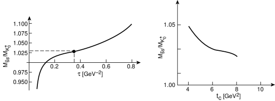
Figure 8: $\tau$ and $t_{c}$ behaviours of $M_{\bar{s}s}/M_{K^{*}_{0}(1.43)}$.

The result indicates the mass hierarchy:

$$M_{S_{2}\equiv\bar{u}u+\bar{d}d}<M_{K^{*}_{0}\equiv\bar{u}s}<M_{\bar{s}s}.$$ (93)

The $SU(3)$ breaking obtained here is slightly larger than the naïve expectation as, in addition to the strange-quark mass effect, the $\langle\bar{s}s\rangle$ condensate also plays an important role in the splitting. The sum rule ${\cal F}_{\bar{s}s}$ leads to the value of the decay constant (Fig. 9):

$$f_{\bar{s}s}=(43\pm 19)~{}\mbox{MeV}.$$ (94)

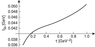
Figure 9: $\tau$ behaviour of the decay constant $f_{\bar{s}s}$.

These previous estimates have been optimized at $t_{c}\simeq 6$ GeV². Therefore, we expect that the radial excitation $S^{\prime}_{3}$ will be in the range:

$$M_{S^{\prime}_{3}}\approx(1.7\sim 2.4)~{}\mbox{GeV},$$ (95)

where the first number corresponds to the phenomenological extrapolation $M_{S^{\prime}_{2}}-M_{S_{2}}\simeq M_{S^{\prime}_{3}}-M_{S_{3}}$, while the second value is $\sqrt{t_{c}}$.

6.4 Couplings of the $S_{3}$ to $K^{+}K^{-}$ and $\gamma\gamma$

In so doing, we work with the vertex (Fig. 10):

$$V(p,q)=\int d^{4}x~{}d^{4}y~{}e^{-ipx}e^{i(p+q)y}\langle 0|{\cal T}J_{K^{+}}(x)J_{K^{-}}(y)J_{\bar{s}s}(0)|0\rangle~{},$$ (96)

and evaluate it at the symmetric point $p^{2}=q^{2}=(p+q)^{2}=-(Q^{2}\geq 0)$ as in [58].

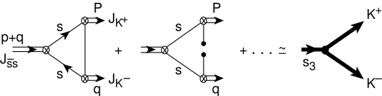
Figure 10: Vertex sum rule for the $S_{3}K^{+}K^{-}$ coupling.

Then, we obtain, in $4-\epsilon$ dimensions:

$$V(-Q^{2})=-m^{2}_{s}\left\{-\frac{3}{2\pi^{2}}m_{s}\Gamma(\epsilon/2)\left(\frac{Q^{2}}{\nu^{2}}\right)^{-\epsilon/2}+\frac{1}{2Q^{2}}\langle\bar{u}u-\bar{s}s\rangle\right\}.$$ (97)

Its phenomenological expression can be approximated by:

$$V(-Q^{2})=\frac{2f_{K}^{2}M^{4}_{K}}{\left(Q^{2}+M^{2}_{K}\right)^{2}}\frac{2f_{\bar{s}s}^{2}M^{4}_{\bar{s}s}}{\left(Q^{2}+M^{2}_{\bar{s}s}\right)}g_{S_{3}K^{+}K^{-}}.$$ (98)

The Laplace transform of the previous equation leads to:

$$g_{S_{3}K^{+}K^{-}}\sqrt{2}M^{2}_{\bar{s}s}f_{\bar{s}s}\int_{0}^{1}xdx~{}e^{-x(M^{2}_{\bar{s}s}-M^{2}_{K})\tau}\simeq 4m_{s}\left\{m_{s}-\frac{\pi^{2}}{3}\tau\langle\bar{u}u-2\bar{s}s\rangle\right\}.$$ (99)

Using [63] $\langle\bar{s}s\rangle/\langle\bar{u}u\rangle\simeq 0.7$, $\langle\bar{u}u\rangle$(1 GeV) $\simeq-(229\mbox{MeV})^{3}$ and $m_{s}$ (1 GeV)$~{}\simeq$ (150$\sim$190) MeV, we obtain:

$$g_{S_{3}K^{+}K^{-}}\simeq(2.7\pm 0.5)~{}\mbox{GeV}~{}~{}~{}\mbox{and}~{}~{}~{}g_{S_{3}\eta\eta}\simeq 0.9\sqrt{\frac{2}{3}}g_{S_{3}K^{+}K^{-}}.$$ (100)

We can also predict:

$$g_{S_{3}\eta\eta^{\prime}}\simeq\sin\theta_{P}g_{S_{3}\eta\eta}.$$ (101)

This result can be compared with the one obtained previously, and with $g_{a_{0}K^{+}K^{-}}\simeq 2$ GeV from [58], which expresses the good SU(3) symmetry of the couplings as intuitively expected. Therefore, we can deduce:

$$\Gamma(S_{3}\rightarrow K^{+}K^{-})\simeq(73\pm 27)~{}\mbox{MeV}~{}~{}~{}\mbox{and}~{}~{}~{}\Gamma(S_{3}\rightarrow\eta\eta)\simeq(15\pm 6)~{}\mbox{MeV}.$$ (102)

A comparison of this result with the $f_{0}(1.5)$ width into $K\bar{K}$ of 5 MeV, and the strong coupling of the $f_{0}(1.5)$ to $\pi\pi$ leads us to the conclusion that this state cannot be a pure $\bar{s}s$ state.
We estimate the $S_{3}\gamma\gamma$ width using its relation with the one of $S_{2}$ and the corresponding quark charge:

$$\Gamma(S_{3}\rightarrow\gamma\gamma)\approx\frac{2}{25}\left(\frac{M_{S_{3}}}{M_{S_{2}}}\right)^{3}\Gamma(S_{2}\rightarrow\gamma\gamma)\approx(0.40\pm 0.04)~{}\mbox{keV}.$$ (103)

Finally, analogous to the case of $S^{\prime}_{2}$, we can also have for $M_{S^{\prime}_{3}}\simeq 1.7$ GeV:

$$\Gamma(S^{\prime}_{3}\rightarrow\gamma\gamma)\approx(1.1\pm 0.5)~{}\mbox{keV},~{}~{}~{}~{}~{}~{}~{}~{}~{}\Gamma(S^{\prime}_{3}\rightarrow K^{+}K^{-})\approx(112\pm 50)~{}\mbox{MeV}.$$ (104)

7 “Mixing-ology” for the decay widths of scalar mesons

We have discussed in the previous sections the masses and widths of the unmixed gluonia and quarkonia states. The small value of the mass mixing angle computed in [2] from the off-diagonal two-point correlator (see Fig. 11), which is proportional to the light quark mass, allows us to neglect the off-diagonal term in the mass matrix, and to identify the physical meson masses with the ones of the unmixed states.

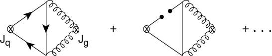
Figure 11: Off-diagonal two-point correlator controlling the quarkonium-gluonium mass mixing angle.

In the following, we shall be concerned with the mixing angle for the couplings, which, in the same approach, is controlled by the off-diagonal non-perturbative three-point function (see Fig. 12) which can (a priori) give a large mixing angle.

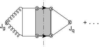
Figure 12: Off-diagonal non-perturbative three-point function controlling the coupling mixing angle in the quarkonium-gluonium decays into pion pairs.

7.1 Mixing below 1 GeV and the nature of the $\sigma$ and $f_{0}(0.98)$

This part will be an update of the scheme proposed by BN [27]. We consider that the physically observed $f_{0}$ and $\sigma$ states result from the two-component mixing of the $\sigma_{B}$ and $S_{2}\equiv\frac{1}{\sqrt{2}}(\bar{u}u+\bar{d}d)$ unmixed bare states:

$$|f_{0}\rangle \equiv -\sin\theta_{S}|\sigma_{B}\rangle+\cos\theta_{S}|S_{2}\rangle$$

$$|\sigma\rangle \equiv ~{}~{}\cos\theta_{S}|\sigma_{B}\rangle+\sin\theta_{S}|S_{2}\rangle.$$ (105)

We also use the previous prediction for $\Gamma({\sigma_{B}}\rightarrow\gamma\gamma)\simeq(0.2\sim 0.3)~{}\mbox{keV},$ and the experimental width $\Gamma(f_{0}\rightarrow\gamma\gamma)\approx 0.3$ keV. Therefore, we can fix the mixing angle to be:

$$\theta_{S}\approx(40\sim 45)^{\circ},$$ (106)

which indicates that the $f_{0}$ and $\sigma$ have a large amount of gluons in their wave function. This situation is quite similar to the case of the $\eta^{\prime}$ in the pseudoscalar channel (mass given by its gluon component, but strong coupling to quarkonia). Using the previous value of $\theta_{S}$, the predicted value of $g_{S_{2}K^{+}K^{-}}$, the approximate relation $g_{S_{2}K^{+}K^{-}}\simeq\frac{1}{2}g_{S_{2}\pi^{+}\pi^{-}}$, and the almost universal coupling of the $\sigma_{B}$ to pairs of Goldstone bosons, one can deduce:

$$g_{f_{0}\pi^{+}\pi^{-}} \simeq (0.1\sim 2.6)~{}\mbox{GeV},~{}~{}~{}~{}~{}~{}g_{f_{0}K^{+}K^{-}}\simeq-(1.3\sim 4.1)~{}\mbox{GeV},$$

$$g_{\sigma\pi^{+}\pi^{-}} \simeq ~{}g_{\sigma K^{+}K^{-}}\simeq(4\sim 5)~{}\mbox{GeV},$$ (107)

which provides a simple explanation of the exceptional property of the $f_{0}$ (strong coupling to $\bar{K}K$ as observed in $\pi\pi$ and $\bar{K}K$ data [65]), without appealing to the more exotic four-quark states and $\bar{K}K$ molecules [66] . Using the previous predictions for the couplings, and for $\theta_{S}$, we obtain for $M_{\sigma_{B}}=(0.75\sim 1.0)$ GeV:

$$\Gamma(f_{0}(0.98)\rightarrow\pi^{+}\pi^{-})\approx(0.2\sim 134)~{}\mbox{MeV}~{}~{}~{}~{}~{}~{}~{}~{}~{}~{}~{}~{}~{}~{}~{}~{}~{}~{}~{}~{}~{}\Gamma(\sigma\rightarrow\pi^{+}\pi^{-})\approx(300\sim 700)~{}\mbox{MeV},$$ (108)

By recapitulating, our scheme suggests that around 1 GeV, there are two mesons that have 1/2 gluon and 1/2 quark in their wave functions resulting from a maximal destructive mixing between a quarkonium ($S_{2}$) and gluonium $(\sigma_{B})$ states:
$\bullet$ The $(a_{0}(0.98))$ is narrow, with a width $\leq$ 134 MeV, and couples strongly to $\bar{K}K$, with the strength
$g_{f_{0}K^{+}K^{-}}/g_{f_{0}\pi^{+}\pi^{-}}\simeq 2$. This property has been seen in $\pi\pi$ and $\gamma\gamma$ scatterings [65] and in $\bar{p}p$ [67] experiments, and also suggests its production from the $\phi$ radiative decay.
$\bullet$ The $\sigma$, with a mass around $0.75\sim 1$ GeV, is large, with a width of about $(300\sim 700)$ MeV.

7.2 Mixing above 1 GeV and the nature of the $f_{0}(1.37)$, $f_{0}(1.5)$ and $f_{J}(1.7)$

7.2.1 The data

Let us recall the experimental facts . Coupled channels analysis demonstrate that in addition to the broad $\sigma(1.0)$ below 1.2 GeV, one needs the $f_{0}(1.37)$, with the following properties [53, 55]:

$$\Gamma(f_{0}(1.37)\rightarrow\mbox{all})\simeq(150\sim 500)~{}\mbox{MeV}~{}~{}~{}~{}~{}~{}~{}~{}\Gamma(f_{0}(1.37)\rightarrow\gamma\gamma)\simeq(5.4\pm 2.3)~{}\mbox{keV},$$ (109)

(where the number for the $\gamma\gamma$ width is less reliable); however, from the quoted branching ratios and extracting the $4\pi$ S-wave, we deduce [53]:

$$\Gamma(f_{0}(1.37)\rightarrow\pi\pi)\leq(15\sim 100)~{}\mbox{MeV},~{}~{}~{}~{}~{}~{}~{}~{}~{}~{}~{}~{}~{}~{}~{}~{}~{}~{}~{}~{}~{}~{}~{}~{}~{}\Gamma(f_{0}(1.37)\rightarrow(4\pi)_{S})\simeq(46\sim 316)~{}\mbox{MeV}.$$ (110)

For the $f_{0}(1.5)$, one has [14, 8]:

$$\Gamma(f_{0}(1.50)\rightarrow~{}\mbox{all})\simeq(100\sim 150)~{}\mbox{MeV},~{}~{}~{}~{}~{}~{}~{}~{}~{}~{}~{}~{}~{}~{}~{}~{}~{}~{}~{}~{}\frac{\Gamma(f_{0}(1.50)\rightarrow 4\pi)}{\Gamma(f_{0}(1.50)\rightarrow\pi\pi)}\simeq(3.4\pm 0.8),$$ (111)

while the partial widths of the $f_{0}(1.5)$ divided by the phase-space factor satisfy the ratios:

$$\pi\pi~{}:~{}\eta\eta~{}:~{}\eta\eta^{\prime}~{}:~{}\bar{K}K\simeq 1~{}:~{}(0.27\pm 0.11)~{}:~{}(0.19\pm 0.08)~{}:~{}(0.24\pm 0.09).$$ (112)

By assuming that the branching ratios other than the previous ones are negligible, we can deduce the experimental data:

$$\Gamma(f_{0}(1.50)\rightarrow\pi\pi) \simeq (20\sim 31)~{}\mbox{MeV}~{}~{}~{}~{}~{}~{}~{}~{}~{}\Gamma(f_{0}(1.50)\rightarrow\bar{K}K)\simeq(3.6\sim 5.6)~{}\mbox{MeV}$$

$$\Gamma(f_{0}(1.50)\rightarrow\eta\eta) \simeq (2.6\sim 3.3)~{}\mbox{MeV}~{}~{}~{}~{}~{}~{}~{}~{}~{}~{}~{}~{}\Gamma(f_{0}(1.50)\rightarrow 4\pi^{0})\simeq(68\sim 105)~{}\mbox{MeV},$$ (113)

and:

$$\Gamma(f_{0}(1.50)\rightarrow\eta\eta^{\prime})\simeq 1.3~{}\mbox{MeV}.$$ (114)

In the region between 1 and 1.5 GeV, we shall be concerned with the four unmixed states: the radial excitations $S^{\prime}_{2}(1.3)$ of the $S_{2}$ and $\sigma^{\prime}_{B}(1.37)$ of the $\sigma_{B}$, the $S_{3}(1.47)$ and the $G(1.5)$.

7.2.2 Nature of the $f_{0}(1.37)$

By inspecting the experimental data in the region around $1.37$ GeV, one can expect that the $f_{0}(1.37)$ which has a large $\gamma\gamma$ width, is a good candidate for being essentially composed by the quarkonium $S^{\prime}_{2}$. However, its large decay width into $4\pi$ indicates its large gluon component from the $\sigma^{\prime}_{B}$. Due to the almost degenerate values of the two previous unmixed states, we expect that they will mix in a maximal way, as in the case of their corresponding ground states $S_{2}-\sigma_{B}$ of mass around 1 GeV. Therefore, we expect that it is difficult to disentangle the effects of these two resonances where:
$\bullet$ The $S^{\prime}_{2}$ quarkonium state is (relatively) narrower with a total width around 400 MeV. It decays mainly into $\pi\pi$ (its decays into $\bar{K}K$ and $\eta\eta$ can be obtained by taking proper Clebsch-Gordan factor and assuming $SU(3)$ symmetry of the couplings.), and has a large $\gamma\gamma$ width of about 4 keV.
$\bullet$ The $\sigma^{\prime}$ is very broad, with a width as large as 1 GeV, has an universal coupling to $\pi\pi$, $\bar{K}K$ and $\eta\eta$, and can decay into $4\pi$ via $\sigma\sigma$, with a width of $(46\sim 316)$ MeV. However, its decay into $\gamma\gamma$ is relatively small.
$\bullet$ The experimental candidate $f_{0}(1.37)$ has amusingly the combined properties of the $S^{\prime}_{2}$ and $\sigma^{\prime}$.

7.2.3 A 3x3 mixing scheme and nature of the $f_{0}(1.5)$

In the following estimate of the hadronic widths of the remaining other mesons, we expect that, due to its large width, the $\sigma^{\prime}$ can have a stronger mixing with the $S_{3}(1.47)$ and the $G(1.5)$, than the $S^{\prime}_{2}$, such that, to a first approximation, we shall only consider the mixing of the three states $\sigma^{\prime}(1.37)$, $S_{3}(1.47)$ and the $G(1.5)$ through the unitary $3\times 3$ CKM-like mixing matrix of the couplings :

$$\left(\begin{array}[]{c}f_{0}(1.37)\\ f_{0}(1.50)\\ f_{0}(1.60)\\ \end{array}\right)=\left(\begin{array}[]{ccc}c_{12}c_{13}&s_{12}c_{13}&s_{13}\\ -s_{12}c_{23}-c_{12}s_{23}s_{13}&c_{12}c_{23}-s_{12}s_{23}s_{13}&s_{23}c_{13}\\ s_{12}s_{23}-c_{12}c_{23}s_{13}&-c_{12}s_{23}-s_{12}c_{23}s_{13}&c_{23}c_{13}\\ \end{array}\right)\left(\begin{array}[]{c}\sigma^{\prime}(1.37)\\ S_{3}(1.47)\\ G(1.5)\\ \end{array}\right)$$ (115)

where:

$$c_{ij}=\cos{\theta_{ij}}~{}~{}~{}~{}\mbox{and}~{}~{}~{}~{}s_{ij}=\sin{\theta_{ij}}.$$ (116)

We shall use in our numerical analysis:

$$\Gamma(\sigma^{\prime}\rightarrow\pi\pi) \approx (1\sim 2)~{}\mbox{GeV}~{}~{}~{}~{}~{}~{}~{}~{}~{}\Gamma(\sigma^{\prime}\rightarrow 4\pi)\approx(40~{}\sim 316)~{}\mbox{MeV (data)},$$

$$\Gamma(\sigma^{\prime}\rightarrow\bar{K}K) \approx (0.7\sim 1.5)~{}\mbox{GeV}~{}~{}~{}~{}~{}~{}~{}~{}~{}\Gamma(\sigma^{\prime}\rightarrow\eta\eta)\approx(0.2\sim 0.4)~{}\mbox{GeV},$$ (117)

and we shall discuss separately the cases of large (upper values) and small (lower values) of each partial widths.

$\bullet$ The case of small widths
We estimate each entry as follows:
For the first line of the matrix, we shall fix $c_{12}$ from the small width of $f_{0}(1.37)$ into $\bar{K}K$, which gives:

$$c_{12}\approx 0.31~{}~{}~{}~{}~{}~{}~{}~{}s_{12}\approx-0.95.$$ (118)

Then , we fix $\theta_{13}$, by requiring the best prediction:

$$\Gamma(f^{B}_{0}(1.37)\rightarrow 4\pi)\approx 150~{}\mbox{MeV}$$ (119)

compared with the previous data. This implies the two solutions (a) and (b):

$$c_{13}\approx~{}~{}~{}\mbox{(a)}~{}~{}~{}-0.29~{}~{}~{}~{}~{}~{}~{}\mbox{and}~{}~{}~{}\mbox{(b)}~{}~{}~{}~{}~{}~{}0.74.$$ (120)

For the second line of the matrix, we use the observed width $\Gamma(f_{0}(1.5)\rightarrow\pi\pi)$, in order to get:

$$c_{23}\approx~{}~{}~{}\mbox{(a)}~{}~{}~{}0.45~{}~{}~{}~{}~{}~{}~{}\mbox{and}~{}~{}~{}\mbox{(b)}~{}~{}~{}~{}~{}~{}0.37.$$ (121)

for the corresponding two values of $c_{13}$. Finally, the observed width $\Gamma(f_{0}(1.5)\rightarrow 4\pi)$ favours the alone case (b).
$\bullet$ The case of large widths
We repeat the previous analysis taking the upper values of the partial widths.
$\bullet$ Predictions
Our final mixing matrix is given by the largest range spanned by each mixing angles. Therefore, the mixing matrix reads:

$$\left(\begin{array}[]{c}f_{0}(1.37)\\ f_{0}(1.50)\\ f_{0}(1.60)\\ \end{array}\right)\approx\left(\begin{array}[]{ccc}0.01\sim 0.22&-(0.44\sim 0.7)&0.89\sim 0.67\\ 0.11\sim 0.16&0.89\sim 0.71&0.43\sim 0.69\\ -(0.99\sim 0.96)&-(0.47\sim 0.52)&0.14\sim 0.27\\ \end{array}\right)\left(\begin{array}[]{c}\sigma^{\prime}(1.37)\\ S_{3}(1.47)\\ G(1.5)\\ \end{array}\right),$$ (122)

where the first (resp. second) numbers correspond to the case of large (resp. small) widths. From the previous schemes, we deduce the predictions :

$$\Gamma(f_{0}(1.37)\rightarrow\pi\pi)\approx(22\sim 48)~{}\mbox{MeV}~{}~{}~{}~{}~{}~{}~{}~{}~{}\Gamma(f_{0}(1.37)\rightarrow\eta\eta)\leq 1.~{}\mbox{MeV}~{}~{}~{}~{}~{}~{}~{}~{}~{}\Gamma(f_{0}(1.37)\rightarrow\eta\eta^{\prime})\leq 2.5~{}\mbox{MeV}$$ (123)

and

$$\Gamma(f_{0}(1.5)\rightarrow\bar{K}K)\approx(3\sim 12)~{}\mbox{MeV}~{}~{}~{}~{}~{}~{}\Gamma(f_{0}(1.5)\rightarrow\eta\eta)\approx(1\sim 2)~{}\mbox{MeV}~{}~{}~{}~{}~{}~{}\Gamma(f_{0}(1.5)\rightarrow\eta\eta^{\prime})\leq 1.~{}\mbox{MeV}~{}.$$ (124)

Despite the crude approximation used and the inaccuracy of the predictions, these results are in good agreement with the data, especially from the Crystal Barrel collaboration. These results suggest that the observed $f_{0}(1.37)$ and $f_{0}(1.5)$ come from a maximal mixing between the gluonia ($\sigma^{\prime}$ and $G$) and the quarkonium $S_{3}$ states. The mixing of the $S_{3}$ and $G$ with the quarkonium $S^{\prime}_{2}$, which we have neglected compared with the $\sigma^{\prime}$, can restore the small discrepancy with the data. One should notice, as already mentioned, that the state seen by GAMS is more likely to be similar to the unmixed gluonium state $G$ (dominance of the $4\pi$ and $\eta\eta^{\prime}$ decays, as emphasized earlier in NV), which can be due to some specific features of the central production (double pomeron exchange mechanism which favours the gluonia production) for the GAMS experiment. This feature is not shared by the data from the Crystal Barrel and Obelix collaborations, which correspond to the annihilation of antiprotons at rest in a hydrogen target, and therefore can also favour the production of quarkonia states .

7.2.4 Nature of the $f_{J}(1.71)$

For the $f_{0}(1.6)$, we obtain:

$$\Gamma(f_{0}(1.6)\rightarrow\bar{K}K) \approx (0.5\sim 1.6)~{}\mbox{GeV}~{}~{}~{}~{}~{}~{}~{}~{}~{}\Gamma(f_{0}(1.6)\rightarrow\pi\pi)\approx(0.9\sim 2.)~{}\mbox{GeV}$$

$$\Gamma(f_{0}(1.6)\rightarrow\eta\eta) \approx (0.04\sim 0.6)~{}\mbox{GeV}~{}~{}~{}~{}~{}~{}~{}~{}\Gamma(f_{0}(1.6)\rightarrow\eta\eta^{\prime})\approx(0.03\sim 0.07)~{}\mbox{GeV},$$ (125)

and

$$\Gamma(f_{0}(1.6)\rightarrow(4\pi)_{S})\approx(0.02\sim 0.2)~{}\mbox{GeV},$$ (126)

which suggest that the $f_{0}(1.6)$ is very broad and can again be confused with the continuum. Therefore, the $f_{J}(1.7)$ observed to decay into $\bar{K}K$ with a width of the order $(100\sim 180)$ MeV, can be essentially composed by the radial excitation $S^{\prime}_{3}(1.7\sim 2.4)$ GeV of the $S_{3}(\bar{s}s)$, as they have about the same width into $\bar{K}K$ (see section 6.4). This can also explain the smallness of the $f_{J}(1.7)$ width into $\pi\pi$ and $4\pi$. Our predictions of the $f_{J}(1.71)$ width can agree with the result of the Obelix collaboration [67], while its small decay width into $4\pi$ is in agreement with the best fit of the Crystal Barrel collaboration (see Abele et al. in [14]), which is consistent with the fact that the $f_{0}(1.37)$ likes to decay into 4$\pi$. However, the $f_{0}(1.6)$ and the $f_{J}(1.71)$ can presumably interfere destructively for giving the dip around $1.5\sim 1.6$ GeV seen in the $\bar{K}K$ mass distribution from the Crystal Barrel and $\bar{p}p$ annihilations at rest [68, 67].

7.2.5 Comparison with other scenarios

One can also compare our results with some other mixing scenarios [69, 70]. Though the relative amount of glue for the $f_{0}(1.37)$ and $f_{0}(1.5)$ is about the same here and in [69] , one should notice that, in our case, the $\pi\pi$ partial width of these mesons come mainly from the $\sigma^{\prime}$, a glue state coupled strongly to the quark degrees of freedom, like the $\eta^{\prime}$ of the $U(1)_{A}$ anomaly, while in [69], the $S_{2}$ which has a mass higher than the one obtained here plays an essential role in the mixing. Moreover, the $f_{J}(1.71)$ differs significantly in the two approaches, as here, the $f_{J}(1.71)$ is mainly the $\bar{s}s$ state $S^{\prime}_{3}$, while in [69], it has a significant gluon component. In the present approach, the eventual presence of a large gluon component into the $f_{J}(1.71)$ wave function can only come from the mixing with the broad $f_{0}(1.6)$ and with the radial excitation of the gluonium $G$(1.5), which mass is expected to be around 2 GeV (value of $\sqrt{t_{c}}$ in the QSSR analysis). However, the apparent absence of the $f_{J}(1.71)$ decay into 4$\pi$ from Crystal Barrel data may not favour such a scenario.

7.2.6 Summary

Within the present approach and the present data, we expect above 1 GeV that:
$\bullet$ the $f_{0}(1.37)$ is a superposition of two states: the radial excitation $S^{\prime}_{2}$ of the quarkonium $S_{2}\equiv(\bar{u}u+\bar{d}d)$ and an $f_{0}(1.37)$ resulting from a maximal mixing between the gluonium $G$ and the $S_{3}(\bar{s}s)$ with the radial excitation $\sigma^{\prime}_{B}$ of the broad low mass $\sigma_{B}$. Its large $\gamma\gamma$ width comes from the $S^{\prime}_{2}$, while its affinity to decaying into $4\pi$ comes essentially from the $\sigma^{\prime}$.
$\bullet$ the $f_{0}(1.5)$ with the properties observed by the Crystal Barrel collaboration results from a maximal mixing between the gluonium $G$ and the $S_{3}(\bar{s}s)$ with the radial excitation $\sigma^{\prime}$ of the broad low-mass $\sigma$. This large gluon component explains its affinity to decaying into $2\pi$ (from $\sigma^{\prime}(1.37)$) and $4\pi$ (from $\sigma^{\prime}$ and $G$)
$\bullet$ the $f_{J}(1.71)$ can be identified with the radial excitation $S^{\prime}_{3}$ of the ground state $S_{3}(1.47)$, as they have about the same width into $\bar{K}K$. This can also explain the absence of its decay into $\pi\pi$ and 4$\pi$. The eventual observation of these decays can measure its expected tiny mixing with the wide (and presumably unobservable) $f_{0}(1.6)$ and with the radial excitation of the $G(1.5)$. The presence of the dip around $(1.5\sim 1.6)$ GeV seen in the $\bar{K}K$ invariant mass distribution may already be a signal of a such mixing. However, we need a clear spin-parity assignement of the $f_{J}(1.71)$ before a definite conclusion on its nature can be drawn.

8 The tensor gluonium

8.1 Mass and decay constant

In this section, we shall study the properties of the $2^{++}$ gluonium. We shall be concerned with the two-point correlator:

$$\psi^{T}_{\mu\nu\rho\sigma} \equiv i\int d^{4}x~{}e^{iqx}\langle 0|{\cal T}\theta^{g}_{\mu\nu}(x)\theta^{g}_{\rho\sigma}(0)^{\dagger}|0\rangle$$ (127)

$$= \frac{1}{2}\left(\eta_{\mu\rho}\eta_{\nu\sigma}+\eta_{\mu\sigma}\eta_{\nu\rho}-\frac{2}{3}\eta_{\mu\nu}\eta_{\rho\sigma}\right)\psi_{T}(q^{2}),$$

where:

$$\eta_{\mu\nu}\equiv g_{\mu\nu}-\frac{q_{\mu}q_{\nu}}{q^{2}}.$$ (128)

To leading order in $\alpha_{s}$ and including the non-perturbative condensates, the QCD expression of the correlator reads [17]:

$$\psi_{T}(q^{2}\equiv-Q^{2})=-\frac{1}{20\pi^{2}}(Q^{4})\log{\frac{Q^{2}}{\nu^{2}}}+\frac{5}{12}\frac{g^{2}}{Q^{4}}\langle 2O_{1}-O_{2}\rangle~{},$$ (129)

where:

$$O_{1}=\left(f_{abc}G_{\mu\alpha}G_{\nu\alpha}\right)^{2}~{}~{}~{}~{}~{}~{}~{}~{}\mbox{and}~{}~{}~{}~{}~{}~{}~{}~{}O_{2}=\left(f_{abc}G_{\mu\nu}G_{\alpha\beta}\right)^{2}.$$ (130)

Using the vacuum saturation hypothesis, one can write:

$$\langle 2O_{1}-O_{2}\rangle\simeq-\frac{3}{16}\langle G^{2}\rangle^{2}.$$ (131)

In order to get the gluonium mass, we work with the ratio of moments:

$${\cal R}_{10}\equiv\frac{{\cal L}_{T}^{(1)}}{{\cal L}_{T}^{(0)}},$$ (132)

as in SN [18]. Its QCD expression reads:

$${\cal R}_{10}\simeq{3\tau^{-1}}\left\{1+\frac{25}{24}\pi^{3}\frac{\tau^{4}}{\alpha_{s}}\langle\alpha_{s}G^{2}\rangle^{2}\right\}.$$ (133)

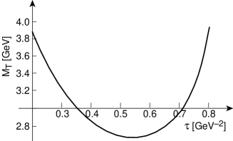
Figure 13: $\tau$ behaviour for the upper bound of the tensor gluonium mass $M_{T}$.

Using the positivity of the spectral function, the minimum of the ratio of the moments (Fig. 13) leads to the upper bound:

$$M_{T}\leq(2.7\pm 0.4)~{}\mbox{GeV},$$ (134)

while a resonance + QCD continuum parametrization of the spectral function gives the value (Fig. 14):

$$M_{T}\simeq(2.0\pm 0.05\pm 0.05\pm 0.05)~{}\mbox{GeV}\simeq(2.0\pm 0.1)~{}\mbox{GeV}.$$ (135)

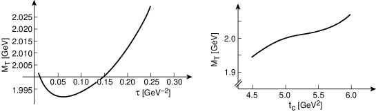
Figure 14: a) $\tau$ and b) $t_{c}$ behaviours of the $2^{++}$ tensor gluonium mass.

The mass obtained here is larger than the one in SN, which is mainly due to the increase of the gluon condensate value. The errors come respectively from the gluon condensate, the factorization assumption and the continuum threshold $t_{c}$. The decay constant can be extracted from ${\cal L}_{T}^{(0)}$, and reads (Fig. 15):

$$f_{T}\simeq(80\pm 8\pm 4\pm 4\pm 10)~{}\mbox{MeV}\simeq(80\pm 14)~{}\mbox{MeV},$$ (136)

where the first error comes from $M_{T}$ and the remaining ones are of the same origin as before.

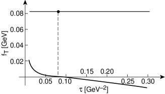
Figure 15: $\tau$ behaviour of the $2^{++}$ tensor gluonium decay constant $f_{T}$.

The value of $t_{c}$ at which these results are optimal is:

$$\sqrt{t_{c}}\approx M_{T^{\prime}}\simeq(2.2\sim 2.3)~{}\mbox{GeV},$$ (137)

which corresponds roughly to the mass of the radial excitation. Our result is slightly higher than the one in SN and in [21], because of the increase of the value of the gluon condensate. We do not expect that the perturbative radiative corrections will affect noticeably our prediction for the mass , as this effect tends to cancel out in the ratio of moments.

8.2 Tensor gluonium decay widths

Using the result in [3], one can constrain the ratio:

$$r\equiv\frac{g_{T\pi\pi}}{g_{f_{2}\pi\pi}}\simeq-(0.68\pm 0.23),$$ (138)

using the data, where:

$$\Gamma({T\rightarrow\pi^{+}\pi-})=\frac{g^{2}_{T\pi\pi}}{30\pi M^{2}_{T}}|k_{\pi}|^{5},$$ (139)

$k_{\pi}$ being the pion momentum. Assuming an universal coupling of the $T$ to the pairs of Goldstone bosons, this leads to the width:

$$\Gamma(T\rightarrow\pi\pi+KK+\eta\eta)\leq(119\pm 36)~{}\mbox{MeV},$$ (140)

which indicates that the $2^{++}$ cannot be wide, contrary to some claims in the literature. Another indication of the smallness of the $2^{++}$ width can be obtained from the low-energy theorem analogue of the one for the scalar gluonium used in section 5 [71]. Using a dipersion relation, one can write:

$$\frac{1}{4}\sum_{f_{2},T}\sqrt{2}f_{T}g_{T\pi\pi}\approx 1.$$ (141)

As in [72], we assume that the vertex is saturated by the $f_{2}(1.27)$ and by the gluonium $T$. Using $f_{f_{2}}\approx 0.19$ GeV [73], the previous value of $f_{T}$, and the experimental value $g_{f_{2}\pi\pi}\simeq 16$ GeV^-1, one can notice that the sum rule is already saturated by the $f_{2}$-meson, and leads to:

$$g_{T\pi\pi}\approx 2.6~{}\mbox{GeV}^{-1}\Longrightarrow\Gamma({T\rightarrow\pi\pi})\approx 10~{}\mbox{MeV},$$ (142)

while taking a typical 10$\%$ error in the estimate of $f_{f_{2}}$, one can deduce:

$$\Gamma({T\rightarrow\pi\pi})\leq 70~{}\mbox{MeV}.$$ (143)

The $\gamma\gamma$ width can be obtained by relating it to the one of the $0^{++}$ gluonium within a non-relativistic quark model approach [3]:

$$\Gamma(T\rightarrow\gamma\gamma)\simeq\frac{4}{15}\left(\frac{M_{T}}{M_{0^{+}}}\right)^{3}\Gamma(0^{++}\rightarrow\gamma\gamma)\simeq 0.06~{}\mbox{keV},$$ (144)

which shows again a small value typical of a gluonium state.

8.3 Meson-gluonium mass mixing and the nature of the $f_{J}(1.71)$ and $\zeta(2.2)$

In order to evaluate the gluonium-quarkonium mass mixing angle, we shall work, as in [2, 3], with the off-diagonal two-point correlator:

$$\psi^{gq}_{\mu\nu\rho\sigma} \equiv i\int d^{4}x~{}e^{iqx}\langle 0|{\cal T}\theta^{g}_{\mu\nu}(x)\theta^{q}_{\rho\sigma}(0)^{\dagger}|0\rangle$$ (145)

$$= \frac{1}{2}\left(\eta_{\mu\rho}\eta_{\nu\sigma}+\eta_{\mu\sigma}\eta_{\nu\rho}-\frac{2}{3}\eta_{\mu\nu}\eta_{\rho\sigma}\right)\psi_{gq}(q^{2}),$$

where

$$\theta^{q}_{\mu\nu}(x)=i\bar{q}(x)(\gamma_{\mu}\overline{D}_{\nu}+\gamma_{\nu}\overline{D}_{\mu})q(x).$$ (146)

Here, $\overline{D}_{\mu}\equiv\overrightarrow{D}_{\mu}-\overleftarrow{D}_{\mu}$ is the covariant derivative, and the other quantities have already been defined earlier. Taking into account the mixing of the currents, one obtains [3]:

$$\psi_{gq}(q^{2}\equiv-Q^{2})\simeq\frac{q^{4}}{15\pi^{2}}\left(\frac{{\alpha_{s}}}{\pi}\right)\left(\log^{2}{\frac{Q^{2}}{\nu^{2}}}-\frac{91}{15}\log{\frac{Q^{2}}{\nu^{2}}}\right)-\frac{7}{36\pi}\log{\frac{Q^{2}}{\nu^{2}}}\langle\alpha_{s}G^{2}\rangle.$$ (147)

The resonance contribution to the spectral function is introduced using a two-component mixing formalism:

$$\frac{1}{\pi}\mbox{Im}\psi_{gq}(t)\simeq\sin{2\theta_{T}}M^{2}_{T}f_{T}M^{2}_{F}f_{F}\delta(t-M^{2})~{}+~{}\mbox{``QCD continuum"},$$ (148)

where $\theta_{T}$ is the mixing angle; $F$ is a generic notation for the quarkonia $f_{2}(1.27)$ and $f^{\prime}_{2}(1.53)$; $M$ is the average of the $G$ and $F$ mass squared; $f_{T,F}$ is the decay constant, where $f_{f_{2}}\simeq(0.11\sim 0.14)M_{f_{2}}$ [72]. Noting that within our approximation, the Laplace transform sum rule does not present a $\tau$ stability, we work with the FESR:

$$\int_{0}^{t_{c}}dt~{}\frac{1}{\pi}\mbox{Im}\psi_{gq}(t)\simeq-\frac{101}{675\pi^{2}}\left(\frac{\bar{\alpha_{s}}}{\pi}\right)t^{3}_{c}\left(1+\frac{525\pi^{2}}{404t^{2}_{c}}\langle G^{2}\rangle\right),$$ (149)

where $t_{c}\simeq\frac{1}{2}(t^{q}_{c}+t^{g}_{c})\simeq 2.2$ GeV² is the average of the continuum threshold for the quark and gluonia channels. Then, one obtains the approximate estimate [3] :

$$\theta_{T}\simeq-10^{\circ},$$ (150)

which is a small mixing angle, and which indicates that:
$\bullet$ the interpretation of the $f_{J}(1.71)$ as the lowest 2⁺⁺ ground state gluonium, is not favoured by our present result.
$\bullet$ the $\zeta(2.2)$ observed by the BES collaboration [74] is a good gluonium candidate (mass and width), but it can be more probably the first radial excitation of the lowest-mass gluonium ($t_{c}\approx 2.2$ GeV). Our result, for the mass, suggests that one needs further data around 2 GeV for finding the lowest mass $2^{++}$ gluonium. Its (non-)finding will be a test for the accuracy of our approach. Our prediction for the mass and for $t_{c}$, which suggests a rich population of $2^{++}$ states in this region, should stimulate a further independent experimental test of the $g_{T}$ candidates seen earlier by the BNL group in the OZI suppressed reaction $\pi^{-}p\rightarrow\phi\phi n$ [75], and a further understanding of their non-observation in $J/\psi$ radiative decays [76].

9 Pseudoscalar gluonia

9.1 Mass and decay constant

The pseudoscalar gluonium sum rules have been discussed many times in the literature, in connection with the gluonium mass in SN [18], $\eta^{\prime}$ meson, the spin of the proton and the slope of the topological $U(1)$ charge in [77, 78]. Here, we update the analysis of the gluonium mass in SN, taking into account the new, large perturbative radiative corrections [48], and the radiative correction for the gluon condensate [25]. In so doing we work with the Laplace transform:

$${\cal L}_{P}^{(0)} \equiv \int_{t_{\leq}}^{\infty}{dt}~{}\mbox{exp}(-t\tau)~{}\frac{1}{\pi}~{}\mbox{Im}\psi_{P}(t)$$ (151)

$$= \left(\frac{1}{8}\right)^{2}\left(\frac{\bar{\alpha_{s}}}{\pi}\right)^{2}\frac{4}{\pi^{2}}\tau^{-3}\Bigg{[}\left(1+\delta_{pert}\left(\frac{\bar{\alpha_{s}}}{\pi}\right)\right)\left(1-\rho_{2}\right)$$

$$-\frac{11\pi}{4}\langle\alpha_{s}G^{2}\rangle\tau^{2}\left(1-\exp(-t_{c}\tau)\right)-2\pi^{2}\tau^{3}g\langle f_{abc}G^{3}_{abc}\rangle\Bigg{]},$$

where:

$$\delta_{pert} \equiv \frac{1}{4}\Bigg{[}83+2\beta_{1}(1-2\gamma_{E})-4\frac{\beta_{1}}{\beta_{2}}\log(-\log{\tau\Lambda^{2}})\Bigg{]}$$

$$\rho_{2} \equiv \left(1+t_{c}\tau+\frac{(t_{c}\tau)^{2}}{2}\right)\exp({-t_{c}\tau})$$ (152)

and the ratio of moments

$${\cal R}_{10}\equiv-\frac{d}{d\tau}\log{{\cal L}_{P}^{(0)}}\equiv\frac{{\cal L}_{P}^{(1)}}{{\cal L}_{P}^{(0)}}.$$ (153)

Subtracting the $\eta^{\prime}$ contribution, and using the positivity of the spectral function, the minimum of ${\cal R}_{10}$ gives the upper bound (Fig. 16):

$$M_{P}\leq(2.34\pm 0.42)~{}\mbox{GeV},$$ (154)

where the error comes mainly from the value of $\Lambda$, which one can understand as the minimum occurring at large values of $\tau$.

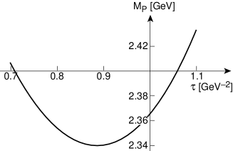
Figure 16: $\tau$ behaviour of the upper bound for the pseudoscalar gluonium mass $M_{P}$.

The estimate of the pseudoscalar gluonia mass is given in Fig. 17, where the stability in $\tau$ is obtained at smaller $\tau$ values, which gives smaller errors. We obtain:

$$M_{P}\simeq(2.05\pm 0.05\pm 0.13\pm 0.13)~{}\mbox{GeV}\simeq(2.05\pm 0.19)~{}\mbox{GeV},$$ (155)

where the first error comes from $t_{c}$, the second and the third ones come from $\Lambda$ and the truncation of the QCD series. As in the previous cases, we have estimated the unknown $\alpha_{s}^{2}$ coefficient to be of the order of $\pm$400 (normalized to the lowest order term) by assuming a geometric growth of the QCD series.

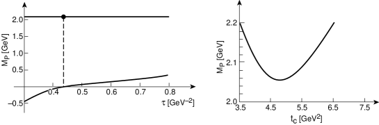
Figure 17: $\tau$ and $t_{c}$ behaviours of the pseudoscalar gluonium mass.

The corresponding value of $t_{c}$ is:

$$\sqrt{t_{c}}\approx M_{P^{\prime}}\simeq(2.1\sim 2.3)~{}\mbox{GeV}.$$ (156)

The decay constant has a good $\tau$ stability (Fig. 18) though the $t_{c}$ stability is only reached at $t_{c}\simeq 7$ GeV² (Fig. 21). Using the range of $t_{c}$ values from 5 to 7 GeV², we deduce:

$$f_{P}\simeq(8\sim 17)~{}\mbox{MeV}.$$ (157)

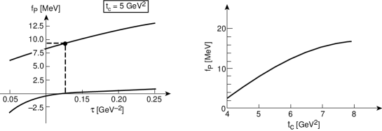
Figure 18: $\tau$ and $t_{c}$ behaviours of the decay constant $f_{P}$ for $t_{c}=5.5$ GeV².

These results are slightly higher than the one in SN obtained from a numerical least-squares fit, because mainly of the effect of the radiative corrections.

9.2 Testing the nature of the $E/\iota(1.44)$

Old [53] and new [79] experimental data indicate the presence of some extra states in the range of 1.40-1.45 GeV, which go beyond the usual nonet classification. In order, to test the nature of such states (denoted hereafter as the $E/\iota(1.44)$), let us now come back to the sum rule:

$${\cal L}_{P}^{(-1)}\equiv\int_{t_{\leq}}^{\infty}\frac{dt}{t}~{}\mbox{exp}(-t\tau)~{}\frac{1}{\pi}~{}\mbox{Im}\psi_{P}(t),$$ (158)

which has been used in [77] for fixing the decay constant $f_{\eta^{\prime}}$:

$$\langle 0|Q(x)|\eta^{\prime}\rangle=\sqrt{2}f_{\eta^{\prime}}M^{2}_{\eta^{\prime}}.$$ (159)

By defining in the same way the decay constant $f_{\iota}$, we introduce into the sum rule the parameters of the $\eta^{\prime}$ and $P$ gluonium and the corresponding value of $t_{c}\simeq 6\sim 7$ GeV² at which $f_{\eta^{\prime}}$ has been optimized. In this way, one finds that there is no room to include the $\iota$ contribution, as:

$$f_{\iota}\approx 0.$$ (160)

One can weaken the constraint by replacing the QCD continuum effect, i.e. all higher-state effects, by the one of the $\iota$, which should lead to an overestimate of $f_{\iota}$. In this way, one can deduce the upper bound (Fig. 19):

$$f_{\iota}\leq 16~{}\mbox{MeV}.$$ (161)

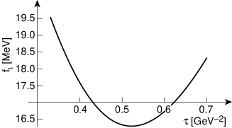
Figure 19: $\tau$ behaviour of the decay constant $f_{\iota}$ for $t_{c}=6.$ GeV²

One can compare the previous result with the one obtained from $J/\psi$ radiative decays, which gives [51]:

$$B_{\iota\eta^{\prime}}\equiv\frac{\Gamma(J/\psi\rightarrow\gamma\iota)}{\Gamma(J/\psi\rightarrow\gamma\eta^{\prime})}\simeq\Bigg{|}\frac{\langle 0|Q(x)|\iota\rangle}{\langle 0|Q(x)|\eta^{\prime}\rangle}\Bigg{|}^{2}\left(\frac{k_{\iota}}{k_{\eta^{\prime}}}\right)^{3},$$ (162)

where the matrix element is controlled by the decay constant of the corresponding particle. Using the experimental branching ratio, where we take the one for $\iota\rightarrow\bar{K}K\pi$, we deduce:

$$f_{\iota}\simeq 0.23f_{\eta^{\prime}}\simeq 7~{}\mbox{MeV},$$ (163)

in agreement with our findings. Our analysis indicates that the $E/\iota$ couples more weakly to the gluonic current than the $\eta^{\prime}$ ($f_{\eta^{\prime}}\approx 30~{}\mbox{MeV}$), and is thus likely to be the radial excitation of the $\eta^{\prime}$ .

9.3 Meson-gluonium mixing and $P\rightarrow\gamma\gamma,\rho\gamma$ decays

Following [2], we obtain from the evaluation of the off-diagonal two-point correlator, the quarkonium-gluonium mixing angle [2, 16]

$$\theta_{P}\simeq 12^{\circ},$$ (164)

from which one can deduce the decay widths of the pseudoscalar gluonium $G$:

$$\Gamma(P\rightarrow\gamma\gamma) \simeq \tan^{2}{\theta_{P}}\left(\frac{M_{P}}{M_{\eta^{\prime}}}\right)^{3}\Gamma(\eta^{\prime}\rightarrow\gamma\gamma)\approx(1.3\pm 0.1)~{}\mbox{keV}$$

$$\Gamma(P\rightarrow\rho\gamma) \simeq \tan^{2}{\theta_{P}}\left(\frac{k_{P}}{k_{\eta^{\prime}}}\right)^{3}\Gamma(\eta^{\prime}\rightarrow\rho\gamma)\approx(0.3\pm 0.1)~{}\mbox{MeV},$$ (165)

where $k_{i}$ is the momentum of the particle $i$. We have used $\Gamma(\eta^{\prime}\rightarrow\gamma\gamma)\simeq 4.3~{}\mbox{keV}$ and $\Gamma(\eta^{\prime}\rightarrow\rho\gamma)\simeq(72\sim 21)~{}\mbox{keV}$. Measurements of the $P$ widths can test the amount of glue inside the $P$-meson.

10 Conclusions

$\bullet$ We have updated the QCD spectral sum rule (QSSR) analysis for computing the masses and decay constants of the scalar (section 4), tensor (section 8) and pseudoscalar (section 9) gluonia, using the present values of the QCD parameters and the recent progresses in the QCD evaluation of the gluonic correlators. The results of the analysis are summarized in Table 1:

$J^{PC}$	Name	Mass [GeV]		$f_{G}$ [MeV]	$\sqrt{t_{c}}$ [GeV]
		Estimate	Upper Bound
$0^{++}$	$G$	$1.5\pm 0.2$	$2.16\pm 0.22$	$390\pm 145$	$2.0\sim 2.1$
	$\sigma_{B}$	1.00 (input)		1000
	$\sigma^{\prime}_{B}$	1.37 (input)		600
	$3G$	3.1		62
$2^{++}$	$T$	$2.0\pm 0.1$	$2.7\pm 0.4$	$80\pm 14$	$2.2$
$0^{-+}$	$P$	$2.05\pm 0.19$	$2.34\pm 0.42$	$8\sim 17$	$2.2$
	$E/\iota$	1.44 (input)		$7~{}:~{}J/\psi\rightarrow\gamma\iota$

Table 1: Unmixed gluonia masses and couplings from QSSR.

Our results satisfy the mass hierarchy $M_{S}<M_{P}\approx M_{T}$, which suggests that the scalar meson is the lightest gluonium state. However, the consistency of the different sum rules in the scalar sector requires the existence of a low mass and broad $\sigma$-meson coupled strongly both to gluons and to pairs of Goldstone bosons, whose effects can be missed in a one-resonance parametrization of the spectral function, and in the present lattice calculations. One should also notice that the values of $\sqrt{t_{c}}$, which are approximately the mass of the next radial excitations, indicate that the mass-splitting between the ground state and the radial excitations is relatively much smaller ($30\%$) than in the case of ordinary hadrons (about $70\%$ for the $\rho$ meson), such that one can expect rich gluonia spectra in the vicinity of 2–2.2 GeV, in addition to the ones of the lowest ground states.
$\bullet$ We have also computed the masses and decay constants of the scalar quarkonia (section 6).
$\bullet$ We have used some low-energy theorems (LET) and/or three-point function sum rules in order to predict some decay widths of the bare unmixed states (sections 5 and 6), where the results are summarized in Table 2 .

Name	Mass [GeV]	$\pi^{+}\pi^{-}$ [GeV]	$K^{+}K^{-}$ [MeV]	$\eta\eta$ [MeV]	$\eta\eta^{\prime}$ [MeV]	$(4\pi)_{S}$ [MeV]	$\gamma\gamma$ [keV]
$\sigma_{B}$	$0.75\sim 1.0$	$0.2\sim 0.5$	$SU(3)$	$SU(3)$			$0.2\sim 0.3$
	(input)
$\sigma^{\prime}_{B}$	1.37	$0.5\sim 1.3$	$SU(3)$	$SU(3)$		$43\sim 316$	$0.7\sim 1.0$
	(input)					(exp)
$G$	1.5	$\approx 0$	$\approx 0$	$1.1\sim 2.2$	$5\sim 10$	$60\sim 138$	$1.0\pm 0.8$
$S_{2}$	1.	0.12	$SU(3)$	$SU(3)$			0.67
$S^{\prime}_{2}$	$1.3\approx\pi^{\prime}$	$0.30\pm 0.15$	$SU(3)$	$SU(3)$			$4\pm 2$
$S_{3}$	$1.474\pm 0.044$		$73\pm 27$	$15\pm 6$			$0.4\pm 0.04$
$S^{\prime}_{3}$	$\approx 1.7$		$112\pm 50$	$SU(3)$			$1.1\pm 0.5$

Table 2: Unmixed scalar gluonia and quarkonia decays

$\bullet$ We have discussed some maximal quarkonium-gluonium mixing schemes, in an attempt to explain the complex structure and decays of the observed scalar mesons:
Below 1 GeV:
We find that, a maximal mixing between two near-by quarkonium $S_{2}(\bar{u}u+\bar{d}d)$ and gluonium $\sigma_{B}$ states around 1 GeV, can explain the large width of the $\sigma(0.75\sim 1.)$, the narrownness of the $f_{0}(0.98)$ and its strong coupling to $\bar{K}K$ (this latter property enables its production from the $\phi$ radiative decay). This scheme being a QCD-based alternative to the four-quark and $\bar{K}K$ molecule scenarios.
Above 1 GeV:
– The $f_{0}(1.37)$ is a superposition of two states, the $S^{\prime}_{2}$ radial excitation of the $S_{2}\equiv(\bar{u}u+\bar{d}d)$ quarkonium state and the $f_{0}(1.37)$ coming from a maximal mixing between the radial excitation $\sigma^{\prime}_{B}$ of broad low-mass $\sigma$ with the quarkonium $S_{3}$ and gluonium $G$.
– The $f_{0}(1.5)$ satisfying the properties observed by the Crystal Barrel collaboration [14] (namely large widths into $4\pi$, $2\pi$ and $\eta\eta^{\prime}$), comes also from a maximal mixing between the radial excitation $\sigma^{\prime}_{B}$ of a broad low-mass $\sigma$ with the quarkonium $S_{3}$ and gluonium $G$ (orthogonal partner of the $f_{0}(1.37)$). Our approach also suggests that the $G(1.6)$ seen earlier by the GAMS collaboration is likely an “almost” pure gluonium state as emphasized earlier in NV.
– The $f_{J}(1.7)$ (if its spin is confirmed to be zero) can be identified with the $S^{\prime}_{3}$ radial excitation of the $S_{3}(\bar{s}s)$ state. The dip found in the $\bar{K}K$ mass distribution by the Crystal Barrel and $\bar{p}p$ annihilation at rest [68, 67] around $(1.5\sim 1.6)$ GeV can result from a destructive mixing between the $f_{J}(1.71)$ and its orthogonal partner, which is very wide.
$\bullet$ In the tensor sector, using a QSSR evaluation of the off-diagonal quark-gluon two-point correlator, one finds, that the quarkonium-gluonium-mass mixing angle is small, of the order of $10^{\circ}$ [3], which can exclude the identification of the $f_{J}(1.71)$ as a $2^{++}$ gluonium , but favours the gluonium nature of the observed $\zeta(2.2)$, where the total width satisfies our upper bound (section 8). However, due to the small value of the QCD continuum threshold, which is about the mass squared of the radial excitation, we expect to have a rich population of $2^{++}$ gluonia in this 2 GeV region. Our result should stimulate a further search of these states and a test of the (non-)existence of the $g_{T}$ seen earlier by the BNL collaboration in the OZI suppressed $\pi^{-}p\rightarrow\phi\phi n$ reaction, but not observed in previous $J/\psi$ radiative decay data [53, 76].
$\bullet$ In the pseudoscalar sector, the quarkonium-gluonium mass-mixing angle is also small (about 12^∘ [2]), which combined with the decay widths of the $\eta^{\prime}(0.96)$ allows us to predict the gluonium into $\gamma\gamma$ width and radiative decays (section 9). Finally, we found that the $E/\iota(1.44)$ is weakly coupled to the gluonic current, which can favour its interpretation as the radial excitation of the $\eta^{\prime}(0.96)$.

References

- [1] M. Gell-Mann, Acta Phys. Aust. Suppl 9 (1972) 733; H. Fritzsch and M. Gell-Mann, XVI Int. Conf. High-Energy Phys., Chicago, Vol 2 (1972) 135; H. Fritzsch and P. Minkowski, Nuovo Cimento 30A (1975) 393.
- [2] S. Narison, N. Pak and N. Paver, Phys. Lett. B147 (1984) 162.
- [3] E. Bagan, A. Bramon and S. Narison, Phys. Lett. B196 (1987) 203.
- [4] M.S. Chanowitz, Proc. of the VI Int. Workshop on - collisions, ed. R. Lander (World Scientific, Singapore, 1984).
- [5] S. Narison and G. Veneziano, Int. J. Mod. Phys A4, 11 (1989) 2751.
- [6] S.S. Gershtein, A.A. Likhoded and Y.D. Prokoshkin, Z. Phys. C24 (1984) 305.
- [7] F. Binon et al., Nuovo Cimento A78 (1983) 13; D. Alde et al., Nucl. Phys. B269 (1988) 485; D. Alde et al., Phys. Lett. B201 (1988) 160.
- [8] R. Landua, Int. High-Energy Phys. Conf., Varsaw, 1996; S. Spanier, QCD96 Euroconference, Montpellier, Nucl. Phys. (Proc. Suppl.) B, A54 (1997); A. Palano, QCD94 Conference, Montpellier, Nucl. Phys. (Proc. Suppl.) B, C39 (1995).
- [9] A. Patel et al., Phys. Rev. Lett. 57 (1986) 1288; T.H. Burnett and S.R. Sharpe, Annu. Rev. Nucl. and Part. Science 40 (1990) 327 and references therein.
- [10] M. Teper, Oxford Univ. preprint OUTP-95-06P (1994); G. Bali et al. Phys. Lett. B309 (1994) 29.
- [11] F. Butler et al. Nucl. Phys. B430 (1994) 179; B421 (1994) 217; J. Sexton, A. Vaccarino and D. Weingarten, Nucl. Phys. Proc. Supp. B42 (1995) 279.
- [12] G. West, QCD96 Euroconference, Montpellier, Nucl. Phys. (Proc. Suppl.) B, A54 (1997) and private communication.
- [13] C. Amsler and F.E. Close, Phys. Lett. B353 (1995) 385; Phys. Rev. D53 (1996) 295.
- [14] C. Amsler et al., Phys. Lett. B342 (1995) 433; B355 (1995) 425; B353 (1995) 571; B358 (1995) 389; B322 (1994) 431; A. Abele et al., Phys. Lett. B380 (1996) 453.
- [15] M.A. Shifman, A.I. Vainshtein and V.I. Zakharov, Nucl. Phys. B147 (1979) 385, 448.
- [16] S. Narison, QCD spectral sum rules, Lecture Notes in Physics, Vol. 26 (1989) ed. World Scientific and book in preparation.
- [17] V.A. Novikov et al., Nucl. Phys. B191 (1981) 301.
- [18] S. Narison, Z. Phys. C26 (1984) 209; Phys. Lett. B125 (1983) 501.
- [19] N.V. Krasnikov, A.A. Pivovarov and N.N. Tavkhelidze, Z. Phys. C19 (1983) 301.
- [20] P. Pascual and R. Tarrach, Phys. Lett. B113 (1982) 495.
- [21] C.A. Dominguez and N. Paver, Z. Phys. C32 (1986) 391; C31 (1986) 591.
- [22] J. Bordes, V. Gimenez, J.A. Penarrocha, Phys. Lett. B223 (1989) 251.
- [23] E. Bagan and T.G. Steele, Phys. Lett. B243 (1990) 413.
- [24] J.I. Latorre, S. Paban and S. Narison, Phys. Lett. B191 (1987) 437.
- [25] D. Asner et al., Phys. Lett. B296 (1992) 171.
- [26] E.E. Boos and A.V. Daineko, Moscow-INR preprint 90-19/165 (1990).
- [27] A. Bramon and S. Narison, Mod. Phys. Lett. A4 (1989) 1113.
- [28] R. Tarrach, Nucl. Phys. B196 (1982) 45; D. Espriu and R. Tarrach, Z. Phys. C16 (1982) 77.
-
[29]
G. Altarelli, TAU94, Montreux,
Nucl. Phys. (Proc. Suppl.) B 40
(1995) 40 ed. L. Rolandi ;
G. Altarelli, G. Ridolfi and P. Nason, Z. Phys. C 68 (1995) 257; M. Neubert, Nucl. Phys. B463 (1996) 511. - [30] E. Braaten, TAU96, Colorado, 1996; C.J. Maxwell, Int. High-Energy Phys. Conf., Varsaw, 1996; C.J. Maxwell and D.G. Tonge, hep-ph/96066392 (1996).
- [31] R. Akhoury and V. Zakharov, QCD96 Euroconference, Montpellier, Nucl. Phys. (Proc. Suppl.) B, A54 (1997); P. Ball, M. Beneke and V.M. Braun, CERN-TH/95-26 (1995) and references therein;
- [32] A.I. Vainshtein and V.I. Zakharov, Phys. Rev. Lett. 73 (1994) 1207; S. Peris and E. de Rafael, hep-ph/9703455 (1997).
- [33] E. Braaten, S. Narison and A. Pich, Nucl. Phys. B373 (1992) 581.
- [34] F. Le Diberder and A. Pich, Phys. Lett. B286 (1992) 147 and B289 (1992) 165.
- [35] A. Pich, QCD94 Conference, Montpellier, Nucl. Phys. (Proc. Suppl.) B, C39 (1995); S. Narison, TAU94, Montreux, 1994; E. Braaten, TAU96, Colorado, 1996.
- [36] F. Le Diberder, QCD94 Conference, Montpellier, Nucl. Phys. (Proc. Suppl.) B, C39 (1995).
- [37] A.L. Kataev and V.V. Starshenko, QCD94 Conference, Montpellier, Nucl. Phys. (Proc. Suppl.) B, C39 (1995); Mod. Phys. Lett. A10, 3 (1995) 235 and private communication from A.L. Kataev.
- [38] P.M. Stevenson, Phys. Rev. D23 (1981) 2916; G. Grunberg, Phys. Lett. B221 (1980) 70; Phys. Rev. D29 (1984) 2315.
- [39] G.N. Hardy, Divergent Series, Oxford University press, (1949).
- [40] S. Narison, Phys. Lett. B361 (1995) 121.
- [41] S. Narison, Phys. Lett. B387 (1996) 162; hep-ph/9609258, Int. High-Energy Phys. Conf., Varsaw, 1996.
- [42] S. Bethke, QCD94 Conference, Montpellier, Nucl. Phys. (Proc. Suppl.) B, C39 (1995); QCD96 Euroconference, Montpellier, Nucl. Phys. (Proc. Suppl.) B, A54 (1997); I. Hinchliffe, Meeting of the American Physical Society, Albuquerque, 1994; M. Schmelling, Int. High-Energy Phys. Conf., Varsaw, 1996.
- [43] M. Girone and M. Neubert, Phys. Rev. Lett. 76 (1996) 3061.
- [44] D. Buskulic et al., Phys. Lett. B307 (1993) 209; R. Stroynowski, TAU94, Montreux (1994); L. Duflot,TAU94, Montreux (1994).
- [45] J.S. Bell and R.A. Bertlmann, Nucl. Phys. B177 (1981) 218; B227 (1983) 435; R.A. Bertlmann, Nucl. Phys. B204 (1982) 387; QCD90 Conference, Montpellier, Nucl. Phys. (Proc. Suppl) B23 (1991).
- [46] S. Narison and E. de Rafael, Phys. Lett. B103 (1981) 87.
- [47] R.A. Bertlmann, G. Launer and E. de Rafael, Nucl. Phys. B250 (1985) 61;
- [48] A.L. Kataev, N.V. Krasnikov and A.A. Pivovarov, Nucl. Phys. B198 (1982) 508; erratum hep-ph/9612326 (1996). It is a pleasure to thank K. Chetyrkin and A.A. Pivovarov for providing the corrected results prior publication.
- [49] N.A. Törnquist, hep-ph/9510256 Proc. HADRON95 Manchester, 1995 and references therein; V.V. Anisovich, QCD96 Euroconference, Montpellier, Nucl. Phys. (Proc. Suppl.) B, A54 (1997) and references therein; A. Bodyulkov and V. Novozhilov, Trieste preprint IC/89/141 (1989); P. Jain, R. Johnson and J. Schechter, Phys. Rev, D35 (1987) 2230; M.D. Scadron, Proc. Hadron95 Manchester (1995).
- [50] M.A. Shifman, Z. Phys. C9 (1981) 347.
- [51] V.A. Novikov et al. Nucl. Phys. B165 (1980) 67.
- [52] E. Witten, Nucl. Phys. B156 (1979) 269; G. Veneziano, Nucl. Phys. B159 (1979) 213.
- [53] R.M. Barnett et al., Phys. Rev. D54 (1996) 1.
- [54] F. Gilman and R. Kauffman, Phys. Rev. D36 (1987) 2761; L. Montanet, Non-Perturbative Methods Conference, Montpellier, 1985, ed. S. Narison, (World Scientific, Singapore, 1985); P. Ball, J.M. Frère and M. Tytgat, hep-ph/9508359 (1995).
- [55] M. Gaspero, Nucl. Phys A562 (1993) 407.
- [56] R.J. Crewther, Phys. Rev. Lett. 28 (1972) 1421; J. Ellis and M.S. Chanowitz, Phys. Lett. B40 (1972) 397; Phys. Rev. D7 (1973) 2490.
- [57] J. Ellis and J. Lanik, Phys. Lett. B150 (1985) 289; S.R. Sharpe, Symposium on High-Energy Interactions, Vanderbilt Univ., 1984.
- [58] S. Narison and N. Paver, Z. Phys. C22 (1984) 69; Phys. Lett. B135 (1984) 159.
- [59] S. Narison, Phys. Lett. B175 (1986) 88.
- [60] C. Becchi et al., Z. Phys. C8 (1981) 335; S. Narison et al. Nucl. Phys. B121 (1983) 365; S.G. Gorishny, A.L. Kataev and S.A. Larin, Phys. Lett. B135 (1984) 457.
- [61] M. Jamin and M. Munz, Phys. Rev. D51 (1995) 5090.
- [62] K.G. Chetyrkin et al., Phys. Rev. D51 (1995) 5090.
- [63] S. Narison, Phys. Lett. B358 (1995) 113.
- [64] W. Lee and D. Weingarten, hep-lat/9608071 (1996).
- [65] K.L. Au, Thesis RALTO32 (1986) unpublished; K.L. Au, D. Morgan and M.R. Pennington, Phys. Lett. B167 (1988) 229; G. Mennessier, Z. Phys. C16 (1983) 241.
- [66] R.L. Jaffe, Phys. Rev. D15 (1977) 267; J. Weinstein and N. Isgur, Phys. Rev. Lett. 48 (1982) 659; Phys. Rev. D27 (1983) 588; D. Wong and K.F. Liu, Phys. Rev. D21 (1980) 2039; N.N. Achasov, J.A. Devyanin and G.N. Shestakov, Z. Phys. C16 (1982) 55.
- [67] V. Ableev et al., Legnaro preprint LNL-INFN (Rep) 105/96 (1996); U. Gastaldi, Legnaro preprint LNL-INFN (Rep) 99/95 (1995).
- [68] A. Abele et al., Phys. Lett. B385 (1996) 425;
- [69] F.E. Close, Proc. LEAP96, Dinkelsbul (1996) (hep-ph/9610426) and references therein.
- [70] A. Lahiri and B. Bagchi, J. Phys. G11 (1985) L147.
- [71] T.M. Aliev and M.A. Shifman, Phys. Lett. B112 (1982) 401.
- [72] S. Narison, Int. High-Energy Phys. Conf., Munich, 1988.
- [73] E. Bagan and S. Narison, Phys. Lett. B241 (1988) 451.
- [74] Li Jin (BES collaboration), Int. High-Energy Phys. Conf., Varsaw, 1996.
- [75] A. Etkin et al., Phys. Lett. B201 (1988) 294; S.J. Lindenbaum, AIP Conf. Proc. 185, ed. S.U. Chung (1989).
- [76] D. Hitlin, BNL Workshop on Glueballs (1988); B. Jean-Marie, High-Energy Physics Int. Conf., Berkeley (1986).
- [77] S. Narison, G. Shore and G. Veneziano, Nucl. Phys. B433 (1995) 209.
- [78] S. Narison, Phys. Lett. B255 (1991) 101.
- [79] L. Montanet (private communication); N. Djaoshvili (Crystal Barrel collaboration), QCD97 Euroconference, Montpellier, 1997; ibid N.S. Cesari (Obelix collaboration).
- [80] G. Farrar, Phys. Rev. D51 (1995) 3904; Phys. Rev. Lett. 76 (1996) 4111 and 4115.
- [81] K. Chetyrkin, Acta Phys. Polon. B28 (1997) 725 and references therein; L.J. Clavelli and L.R. Surguladze, Phys. Rev. Lett. 78 (1997) 1632.
- [82] F. Csikor and Z. Fodor, Phys. Rev. Lett. 78 (1997) 4335.
- [83] G. Dissertori, QCD97 Euroconference, Montpellier, 1997.