Abstract

The phenomenon of CP violation in the $B$ system and strategies for extracting CKM phases are reviewed. We focus both on general aspects and on some recent developments including CP-violating asymmetries in $B_{d}$ decays, the $B_{s}$ system in light of a possible width difference $\Delta\Gamma_{s}$, charged $B$ decays, and $SU(3)$ relations among certain transition amplitudes. In order to describe the relevant non-leptonic $B$ decays, low energy effective Hamiltonians calculated beyond the leading logarithmic approximation are used. Special emphasis is given to the role of electroweak penguin operators in such transitions. These effects are analyzed both within a general framework and more specifically in view of the theoretical cleanliness of methods to determine CKM phases. Strategies for obtaining insights into the world of electroweak penguins are discussed.

To appear in International Journal of Modern Physics A

International Journal of Modern Physics A,
c  World Scientific Publishing Company

1

CP VIOLATION AND THE ROLE OF ELECTROWEAK

PENGUINS IN NON-LEPTONIC B DECAYS

ROBERT FLEISCHER

Institut für Theoretische Teilchenphysik, Universität Karlsruhe

D–76128 Karlsruhe, Germany

Received (received date)
Revised (revised date)

The phenomenon of CP violation in the $B$ system and strategies for extracting CKM phases are reviewed. We focus both on general aspects and on some recent developments including CP-violating asymmetries in $B_{d}$ decays, the $B_{s}$ system in light of a possible width difference $\Delta\Gamma_{s}$, charged $B$ decays, and $SU(3)$ relations among certain transition amplitudes. In order to describe the relevant non-leptonic $B$ decays, low energy effective Hamiltonians calculated beyond the leading logarithmic approximation are used. Special emphasis is given to the role of electroweak penguin operators in such transitions. These effects are analyzed both within a general framework and more specifically in view of the theoretical cleanliness of methods to determine CKM phases. Strategies for obtaining insights into the world of electroweak penguins are discussed.

1 Setting the Scene

Although the experimental discovery of CP violation by Christenson, Cronin, Fitch and Turlay^? goes back to the year 1964, the non-conservation of the CP symmetry still remains one of the unsolved mysteries in particle physics.

1.1 CP Violation in the $K$-System

So far CP violation has been observed only within the neutral $K$-meson system, where it is described by two complex quantities called $\varepsilon$ and $\varepsilon^{\prime}$ which are defined by the following ratios of decay amplitudes:

$$\frac{A(K_{\mbox{{\scriptsize L}}}\to\pi^{+}\pi^{-})}{A(K_{\mbox{{\scriptsize S}}}\to\pi^{+}\pi^{-})}=\varepsilon+\varepsilon^{\prime},\quad\frac{A(K_{\mbox{{\scriptsize L}}}\to\pi^{0}\pi^{0})}{A(K_{\mbox{{\scriptsize S}}}\to\pi^{0}\pi^{0})}=\varepsilon-2\varepsilon^{\prime}.$$ (1)

While $\varepsilon=(2.26\pm 0.02)\cdot e^{i\frac{\pi}{4}}\cdot 10^{-3}$ parametrizes “indirect” CP violation originating from the fact that the mass eigenstates of the neutral $K$-meson system are not eigenstates of the CP operator, the quantity Re$(\varepsilon^{\prime}/\varepsilon)$ provides a measure of “direct” CP violation in $K\to\pi\pi$ transitions. Unfortunately the experimental situation concerning Re$(\varepsilon^{\prime}/\varepsilon)$, which has been subject of very involved experiments performed both at CERN and Fermilab by the the NA31 and E731 collaborations, respectively, is unclear at present. Whereas NA31 finds^? Re$(\varepsilon^{\prime}/\varepsilon)=(23\pm 7)\cdot 10^{-4}$ indicating already direct CP violation, the result^? Re$(\varepsilon^{\prime}/\varepsilon)=(7.4\pm 5.9)\cdot 10^{-4}$ of the Fermilab experiment E731 provides no unambiguous evidence for a non-zero effect. In about two years this situation is hopefully clarified by the improved measurements at the $10^{-4}$ level of these two collaborations as well as by the KLOE experiment^? at DA$\Phi$NE.

Theoretical analyses^? of Re$(\varepsilon^{\prime}/\varepsilon)$ are very difficult and suffer from large hadronic uncertainties. They are, however, consistent with present experimental data. Because of this rather unfortunate theoretical situation, the measurement of a non-vanishing value of Re$(\varepsilon^{\prime}/\varepsilon)$ will not provide a powerful quantitative test of our theoretical description of CP violation. Consequently the major goal of a possible future observation of Re$(\varepsilon^{\prime}/\varepsilon)\not=0$ would be the exclusion of “superweak” theories^? of CP violation predicting a vanishing value of that quantity.

1.2 The Standard Model Description of CP Violation

At present the observed CP-violating effects arising in the neutral $K$-meson system can be described successfully by the Standard Model (SM) of electroweak interactions^?. Within that framework CP violation is closely related to the quark-mixing-matrix – the Cabibbo–Kobayashi–Maskawa matrix^?,? (CKM matrix) – connecting the electroweak eigenstates $(d^{\prime},s^{\prime},b^{\prime})$ of the $d$-, $s$- and $b$-quarks with their mass eigenstates $(d,s,b)$ through the following unitary transformation:

$$\left(\begin{array}[]{c}d^{\prime}\\ s^{\prime}\\ b^{\prime}\end{array}\right)=\left(\begin{array}[]{ccc}V_{ud}&V_{us}&V_{ub}\\ V_{cd}&V_{cs}&V_{cb}\\ V_{td}&V_{ts}&V_{tb}\end{array}\right)\cdot\left(\begin{array}[]{c}d\\ s\\ b\end{array}\right)\equiv\hat{V}_{\mbox{{\scriptsize CKM}}}\cdot\left(\begin{array}[]{c}d\\ s\\ b\end{array}\right).$$ (2)

The elements of the CKM matrix describe charged-current couplings as can be seen easily by expressing the non-leptonic charged-current interaction Lagrangian

$${\cal L}_{\mbox{{\scriptsize int}}}^{\mbox{{\scriptsize CC}}}=-\frac{g_{2}}{\sqrt{2}}\left(\begin{array}[]{ccc}\bar{u}_{\mbox{{\scriptsize L}}},&\bar{c}_{\mbox{{\scriptsize L}}},&\bar{t}_{\mbox{{\scriptsize L}}}\end{array}\right)\gamma^{\mu}\left(\begin{array}[]{c}d^{\prime}_{\mbox{{\scriptsize L}}}\\ s^{\prime}_{\mbox{{\scriptsize L}}}\\ b^{\prime}_{\mbox{{\scriptsize L}}}\end{array}\right)W_{\mu}^{\dagger}\quad+\quad h.c.$$ (3)

in terms of the electroweak eigenstates (2):

$${\cal L}_{\mbox{{\scriptsize int}}}^{\mbox{{\scriptsize CC}}}=-\frac{g_{2}}{\sqrt{2}}\left(\begin{array}[]{ccc}\bar{u}_{\mbox{{\scriptsize L}}},&\bar{c}_{\mbox{{\scriptsize L}}},&\bar{t}_{\mbox{{\scriptsize L}}}\end{array}\right)\gamma^{\mu}\,\hat{V}_{\mbox{{\scriptsize CKM}}}\left(\begin{array}[]{c}d_{\mbox{{\scriptsize L}}}\\ s_{\mbox{{\scriptsize L}}}\\ b_{\mbox{{\scriptsize L}}}\end{array}\right)W_{\mu}^{\dagger}\quad+\quad h.c.,$$ (4)

where the gauge coupling $g_{2}$ is related to the gauge group $SU(2)_{\mbox{{\scriptsize L}}}$ and the $W_{\mu}^{(\dagger)}$ field corresponds to the charged $W$-bosons. Since neutrinos are massless within the SM, the analogue of the CKM matrix in the leptonic sector is equal to the unit matrix. Furthermore, since the CKM matrix is unitary in flavor-space, flavor changing neutral current (FCNC) processes are absent at tree-level within the SM. Therefore the unitarity of the CKM matrix is the basic requirement of the “GIM-mechanism” describing that feature^?.

The elements of the CKM matrix are fundamental parameters of the SM and have to be extracted from experimental data. Whereas a single real parameter – the Cabibbo angle $\Theta_{\mbox{{\scriptsize C}}}$ – suffices to parametrize the CKM matrix in the case of two fermion generations^?, three generalized Cabibbo-type angles and a single complex phase are needed in the three generation case^?. This complex phase is the origin of CP violation within the SM. Concerning phenomenological applications, the following parametrization of the CKM matrix, which exhibits nicely the hierarchical structure of its elements, is particularly useful:

$$\hat{V}_{\mbox{{\scriptsize CKM}}}=\left(\begin{array}[]{ccc}1-\frac{1}{2}\lambda^{2}&\lambda&A\lambda^{3}(\rho-i\,\eta)\\ -\lambda&1-\frac{1}{2}\lambda^{2}&A\lambda^{2}\\ A\lambda^{3}(1-\rho-i\,\eta)&-A\lambda^{2}&1\end{array}\right)+\,{\cal O}(\lambda^{4}).$$ (5)

The basic idea of that parametrization, which is due to Wolfenstein^?, is a phenomenological expansion of the CKM matrix in powers of the small quantity $\lambda\equiv|V_{us}|=\sin\theta_{\mbox{{\scriptsize C}}}\approx 0.22$. A treatment of the neglected higher order terms can be found e.g. in Refs.^?,?.

Since at present only a single CP-violating observable, i.e. $\varepsilon$, has to be fitted, many different “non-standard” model descriptions of CP violation are imaginable. Since $\varepsilon^{\prime}/\varepsilon$ is also not in a good shape to give an additional stringent constraint, the $K$-meson system by itself cannot provide a powerful test of the CP-violating sector of the SM.

1.3 The Unitarity Triangle

As we will work out in detail in this review, the $B$-meson system represents a very fertile ground for testing the SM description of CP violation. Concerning such tests, the central target is the “unitarity triangle” which is a graphical illustration of the fact that the CKM matrix is unitary^?. The unitarity of the CKM matrix is expressed by

$$\hat{V}_{\mbox{{\scriptsize CKM}}}^{\,\,\dagger}\cdot\hat{V}_{\mbox{{\scriptsize CKM}}}=\hat{1}=\hat{V}_{\mbox{{\scriptsize CKM}}}\cdot\hat{V}_{\mbox{{\scriptsize CKM}}}^{\,\,\dagger}$$ (6)

and leads to a set of twelve equations, where six equations are related to the normalization of the columns and rows of the CKM matrix, and the remaining six equations describe the orthogonality of different columns and rows, respectively. The orthogonality relations are of particular interest since they can be represented as triangles in the complex plane^?. It can be shown that all of these triangles have the same area^?, however, only in two of them all three sides are of comparable magnitude ${\cal O}(\lambda^{3})$, while in the others one side is suppressed relative to the remaining ones by ${\cal O}(\lambda^{2})$ or ${\cal O}(\lambda^{4})$. The latter four triangles are therefore rather squashed ones and hence play a minor phenomenological role. A closer look at the two non-squashed triangles shows that they agree at leading order in the Wolfenstein expansion so that one actually has to deal with a single triangle – the unitarity triangle (UT) of the CKM matrix – that is described by

$$V_{ub}^{\ast}-\lambda V_{cb}^{\ast}+V_{td}=0.$$ (7)

Here terms of ${\cal O}(\lambda^{5})$ have been neglected. Expressing (7) in terms of the Wolfenstein parameters^? and rescaling all sides of the corresponding triangle by $A\lambda^{3}$ gives

$$(\rho+i\,\eta)-1+(1-\rho-i\,\eta)=0.$$ (8)

Consequently the UT can be represented in the complex $(\rho,\eta)$ plane as has been shown in Fig. 1. Defining the UT more strictly through

Figure 1: The unitarity triangle of the CKM matrix in the $(\rho,\eta)$ plane.

$$V_{ud}V_{ub}^{\ast}+V_{cd}V_{cb}^{\ast}+V_{td}V_{tb}^{\ast}=0,$$ (9)

which is the exact CKM phase convention independent definition, the upper corner $A$ of the triangle depicted in that figure receives corrections of ${\cal O}(\lambda^{2})$. In Ref.^? it was pointed out that these corrections can be included straightforwardly by replacing $\rho\to\bar{\rho}\equiv\rho(1-\lambda^{2}/2)$ and $\eta\to\bar{\eta}\equiv\eta(1-\lambda^{2}/2)$. To an accuracy of 3% we have $\bar{\rho}=\rho$, $\bar{\eta}=\eta$ and as far as the phenomenological applications discussed in this review are concerned these corrections are inessential.

The Wolfenstein parametrization (5) can be modified as follows to make the dependence on the angles $\beta$ and $\gamma$ of the UT explicit:

$$\hat{V}_{\mbox{{\scriptsize CKM}}}=\left(\begin{array}[]{ccc}1-\frac{1}{2}\lambda^{2}&\lambda&A\lambda^{3}R_{b}\,e^{-i\gamma}\\ -\lambda&1-\frac{1}{2}\lambda^{2}&A\lambda^{2}\\ A\lambda^{3}R_{t}\,e^{-i\beta}&-A\lambda^{2}&1\end{array}\right)+\,{\cal O}(\lambda^{4}),$$ (10)

where

$$A\equiv\frac{1}{\lambda^{2}}\left|V_{cb}\right|,\,\,R_{b}\equiv\frac{1}{\lambda}\left|\frac{V_{ub}}{V_{cb}}\right|=\sqrt{\rho^{2}+\eta^{2}},\,\,R_{t}\equiv\frac{1}{\lambda}\left|\frac{V_{td}}{V_{cb}}\right|=\sqrt{(1-\rho)^{2}+\eta^{2}}.$$ (11)

The presently allowed ranges^? for these parameters are $A=0.810\pm 0.058$, $R_{b}=0.363\pm 0.073$ and $R_{t}={\cal O}(1)$. The status of $R_{t}$ and strategies to fix this CKM factor have been summarized recently in Ref.^?. Note that the $3^{\mbox{{\scriptsize rd}}}$ angle $\alpha$ of the UT can be obtained straightforwardly through the relation

$$\alpha+\beta+\gamma=180^{\circ}.$$ (12)

At present the UT can only be constrained indirectly through experimental data from CP-violating effects in the neutral $K$-meson system, $B^{0}_{d}-\overline{B^{0}_{d}}$ mixing, and from certain tree decays measuring $|V_{cb}|$ and $|V_{ub}|/|V_{cb}|$. Such analyses have been performed by many authors and can be found e.g. in Refs.^?,?,?,?. It should, however, be possible to determine the three angles $\alpha$, $\beta$ and $\gamma$ of the UT independently in a direct way at future $B$ physics facilities^?-? by measuring CP-violating effects in $B$ decays. Obviously one of the most exciting questions related to these measurements is whether the results for $\alpha$, $\beta$, $\gamma$ will agree one day or not. The latter possibility would signal “New Physics” ^? beyond the SM.

1.4 Outline of the Review

In view of these experiments starting at the end of this millennium it is mandatory for theorists working on $B$ physics to search for decays that should allow interesting insights both into the mechanism of CP violation and into the structure of electroweak interactions in general. A review of such studies is the subject of the present article (for a very compact version see Ref.^?) which is organized as follows:

Since non-leptonic $B$-meson decays play the central role in respect to CP violation and extracting angles of the UT, let us have a closer look at these transitions in Section 2. A very useful tool to analyze such decays are low energy effective Hamiltonians evaluated in renormalization group improved perturbation theory. The general structure of these Hamiltonians consisting of perturbatively calculable Wilson coefficient functions and local four-quark operators is presented in that section, and the problems caused by renormalization scheme dependences arising beyond the leading logarithmic approximation as well as their cancellation in the physical transition amplitudes are discussed.

Section 3 is devoted to CP violation in non-leptonic $B$-meson decays and reviews strategies for extracting the angles of the UT. Both general aspects, a careful discussion of the “benchmark modes” to determine $\alpha$, $\beta$ and $\gamma$, some recent developments including CP-violating asymmetries in $B_{d}$ decays, the $B_{s}$ system in light of a possible width difference $\Delta\Gamma_{s}$, charged $B$ decays, and relations among certain non-leptonic $B$ decay amplitudes are discussed.

In Sections 4 and 5 we shall focus on electroweak penguin effects in non-leptonic $B$ decays and in strategies for extracting CKM phases, respectively. This issue led to considerable interest in the recent literature. Naïvely one would expect that electroweak penguins should only play a minor role since the ratio $\alpha/\alpha_{s}={\cal O}(10^{-2})$ of the QED and QCD couplings is very small. However, because of the large top-quark mass, electroweak penguins may nevertheless become important and may even compete with QCD penguins. These effects are discussed within a general framework in Section 4. There we will see that some non-leptonic $B$ decays are affected significantly by electroweak penguins and that a few of them should even be dominated by these contributions. The question to what extent the usual strategies for extracting angles of the UT are affected by the presence of electroweak penguins is addressed in Section 5. There also methods for obtaining experimental insights into the world of electroweak penguins are discussed.

Finally in Section 6 a brief summary and some concluding remarks are given.

2 Non-leptonic $B$ Decays and Low Energy Effective Hamiltonians

The subject of this section is an introduction to a very useful tool to deal with non-leptonic $B$ decays: low energy effective Hamiltonians. Since the evaluation of these operators beyond the leading logarithmic approximation has been reviewed in great detail by Buchalla, Buras and Lautenbacher in a recent paper^?, only the general structure of these Hamiltonians is discussed here. For the technicalities the reader is referred to Ref.^?. Before turning to these Hamiltonians, let us classify briefly non-leptonic $B$ decays in the following subsection.

2.1 Classification of Non-leptonic $B$ Decays

Non-leptonic $B$ decays are caused by $b$-quark transitions of the type $b\to q_{1}\,\overline{q}_{2}\,q_{3}$ with $q_{1}\in\{d,s\}$ and $q_{2},q_{3}\in\{u,d,c,s\}$ and can be divided into three classes:

• $q_{2}=q_{3}\in\{u,c\}$: both tree and penguin diagrams contribute.

• $q_{2}=q_{3}\in\{d,s\}$: only penguin diagrams contribute.

• $q_{2}\not=q_{3}\in\{u,c\}$: only tree diagrams contribute.

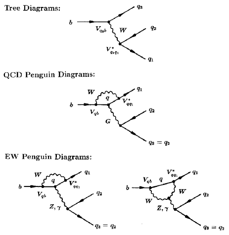
Figure 2: Lowest order contributions to non-leptonic $b$-quark decays $(q\in\{u,c,t\})$.

The corresponding lowest order Feynman diagrams are shown in Fig. 2. There are two types of penguin topologies: gluonic (QCD) and electroweak (EW) penguins originating from strong and electroweak interactions, respectively. Such penguin diagrams play also an important role in the $K$-meson system. The corresponding operators were introduced there by Vainshtein, Zakharov and Shifman^?.

Concerning CP violation, decay classes i) and ii) are very promising. These modes, which are usually referred to as $|\Delta B|=1$, $\Delta C=\Delta U=0$ transitions, will hence play the major role in Section 3. Since we shall analyze such transitions by using low energy effective Hamiltonians calculated in renormalization group improved perturbation theory, let us have a closer look at these operators in the following subsection. Decays belonging to class iii) allow in some cases clean extractions of the angle $\gamma$ of the UT without any hadronic uncertainties and are therefore also very important. The structure of their low energy effective Hamiltonians can be obtained straightforwardly from the $|\Delta B|=1$, $\Delta C=\Delta U=0$ case.

2.2 Low Energy Effective Hamiltonians

In order to evaluate low energy effective Hamiltonians, one makes use of the operator product expansion^? (OPE) yielding transition matrix elements of the structure

$$\langle f|{\cal H}_{\mbox{{\scriptsize eff}}}|i\rangle\propto\sum_{k}\langle f|Q_{k}(\mu)|i\rangle\,C_{k}(\mu),$$ (13)

where $\mu$ denotes an appropriate renormalization scale. The OPE allows one to separate the “long-distance” contributions to that decay amplitude from the “short-distance” parts. Whereas the former pieces are related to non-perturbative hadronic matrix elements $\langle f|Q_{k}(\mu)|i\rangle$, the latter ones are described by perturbatively calculable Wilson coefficient functions $C_{k}(\mu)$.

In the case of $|\Delta B|=1$, $\Delta C=\Delta U=0$ transitions we have

$${\cal H}_{\mbox{{\scriptsize eff}}}={\cal H}_{\mbox{{\scriptsize eff}}}(\Delta B=-1)+{\cal H}_{\mbox{{\scriptsize eff}}}(\Delta B=-1)^{\dagger}$$ (14)

with

$${\cal H}_{\mbox{{\scriptsize eff}}}(\Delta B=-1)=\frac{G_{\mbox{{\scriptsize F}}}}{\sqrt{2}}\left[\sum\limits_{j=u,c}V_{jq}^{\ast}V_{jb}\left\{\sum\limits_{k=1}^{2}Q_{k}^{jq}\,C_{k}(\mu)+\sum\limits_{k=3}^{10}Q_{k}^{q}\,C_{k}(\mu)\right\}\right].$$ (15)

Here $G_{\mbox{{\scriptsize F}}}$ denotes the Fermi constant, the renormalization scale $\mu$ is of ${\cal O}(m_{b})$, the flavor label $q\in\{d,s\}$ corresponds to $b\to d$ and $b\to s$ transitions, respectively, and $Q_{k}^{jq}$ are four-quark operators that can be divided into three categories:

• current-current operators:

  $$\begin{array}[]{rcl}Q_{1}^{jq}&=&(\bar{q}_{\alpha}j_{\beta})_{\mbox{{\scriptsize V--A}}}(\bar{j}_{\beta}b_{\alpha})_{\mbox{{\scriptsize V--A}}}\\ Q_{2}^{jq}&=&(\bar{q}_{\alpha}j_{\alpha})_{\mbox{{\scriptsize V--A}}}(\bar{j}_{\beta}b_{\beta})_{\mbox{{\scriptsize V--A}}}.\end{array}$$ (16)

• QCD penguin operators:

  $$\begin{array}[]{rcl}Q_{3}^{q}&=&(\bar{q}_{\alpha}b_{\alpha})_{\mbox{{\scriptsize V--A}}}\sum_{q^{\prime}}(\bar{q}^{\prime}_{\beta}q^{\prime}_{\beta})_{\mbox{{\scriptsize V--A}}}\\ Q_{4}^{q}&=&(\bar{q}_{\alpha}b_{\beta})_{\mbox{{\scriptsize V--A}}}\sum_{q^{\prime}}(\bar{q}^{\prime}_{\beta}q^{\prime}_{\alpha})_{\mbox{{\scriptsize V--A}}}\\ Q_{5}^{q}&=&(\bar{q}_{\alpha}b_{\alpha})_{\mbox{{\scriptsize V--A}}}\sum_{q^{\prime}}(\bar{q}^{\prime}_{\beta}q^{\prime}_{\beta})_{\mbox{{\scriptsize V+A}}}\\ Q_{6}^{q}&=&(\bar{q}_{\alpha}b_{\beta})_{\mbox{{\scriptsize V--A}}}\sum_{q^{\prime}}(\bar{q}^{\prime}_{\beta}q^{\prime}_{\alpha})_{\mbox{{\scriptsize V+A}}}.\end{array}$$ (17)

• EW penguin operators:

  $$\begin{array}[]{rcl}Q_{7}^{q}&=&\frac{3}{2}(\bar{q}_{\alpha}b_{\alpha})_{\mbox{{\scriptsize V--A}}}\sum_{q^{\prime}}e_{q^{\prime}}(\bar{q}^{\prime}_{\beta}q^{\prime}_{\beta})_{\mbox{{\scriptsize V+A}}}\\ Q_{8}^{q}&=&\frac{3}{2}(\bar{q}_{\alpha}b_{\beta})_{\mbox{{\scriptsize V--A}}}\sum_{q^{\prime}}e_{q^{\prime}}(\bar{q}_{\beta}^{\prime}q^{\prime}_{\alpha})_{\mbox{{\scriptsize V+A}}}\\ Q_{9}^{q}&=&\frac{3}{2}(\bar{q}_{\alpha}b_{\alpha})_{\mbox{{\scriptsize V--A}}}\sum_{q^{\prime}}e_{q^{\prime}}(\bar{q}^{\prime}_{\beta}q^{\prime}_{\beta})_{\mbox{{\scriptsize V--A}}}\\ Q_{10}^{q}&=&\frac{3}{2}(\bar{q}_{\alpha}b_{\beta})_{\mbox{{\scriptsize V--A}}}\sum_{q^{\prime}}e_{q^{\prime}}(\bar{q}^{\prime}_{\beta}q^{\prime}_{\alpha})_{\mbox{{\scriptsize V--A}}}.\end{array}$$ (18)

Here $\alpha$ and $\beta$ denote $SU(3)_{\mbox{{\scriptsize C}}}$ color indices, V$\pm$A refers to the Lorentz structures $\gamma_{\mu}(1\pm\gamma_{5})$, respectively, $q^{\prime}$ runs over the quark flavors being active at the scale $\mu={\cal O}(m_{b})$, i.e. $q^{\prime}\in\{u,d,c,s\}$, and $e_{q^{\prime}}$ are the corresponding electrical quark charges. The current-current, QCD and EW penguin operators are related to the tree, QCD and EW penguin processes depicted in Fig. 2.

In the case of transitions belonging to class iii), only current-current operators contribute. The structure of the corresponding low energy effective Hamiltonians is completely analogous to (15). We have simply to replace both the CKM factors $V_{jq}^{\ast}V_{jb}$ and the flavor contents of the current-current operators (16) straightforwardly, and have to omit the sum over penguin operators. We shall come back to the resulting Hamiltonians^?,?,? in our discussion of $B_{s}$ decays originating from $\bar{b}\to\bar{u}c\bar{s}$ ($b\to c\bar{u}s$) quark-level transitions that is presented in 3.4.5.

The Wilson coefficient functions $C_{k}(\mu)$ can be calculated in renormalization group improved perturbation theory. Within that framework the Wilson coefficients are evolved from a scale of the order of the $W$-boson mass $M_{W}$ down to $\mu={\cal O}(m_{b})$ by solving the renormalization group equations. The use of the renormalization group technique allows one to sum up large logarithms $\log(M_{W}/\mu)$. In the leading logarithmic approximation (LO) terms of the type $(\alpha_{s}\log(M_{W}/\mu))^{n}$ are summed, in the next-to-leading logarithmic approximation (NLO) also terms $(\alpha_{s})^{n}(\log(M_{W}/\mu))^{n-1}$ are summed, and so on. That procedure has been described extensively in an excellent recent review^?, where all technicalities can be found. Let us therefore not go into details except one important feature discussed in the following subsection.

2.3 Renormalization Scheme Dependences

Beyond LO problems arise from renormalization scheme dependences which are reflected by the fact that the Wilson coefficient functions $C_{k}(\mu)$ depend both on the form of the operator basis specified in (16)-(18) and on the scheme to renormalize the matrix elements of the corresponding operators^?. In order to study the cancellation of these scheme dependences explicitly, it is convenient to introduce the following renormalization scheme independent Wilson coefficient functions^?:

$$\overline{\vec{C}}(\mu)=\left[\hat{1}+\frac{\alpha_{s}(\mu)}{4\pi}\hat{r}^{T}_{s}+\frac{\alpha}{4\pi}\hat{r}^{T}_{e}\right]\cdot\vec{C}(\mu).$$ (19)

Here the scheme dependence of $\vec{C}(\mu)$ is cancelled through the one of the scheme dependent matrices $\hat{r}^{T}_{s}$ and $\hat{r}^{T}_{e}$. Using this parametrization we find

$$\vec{Q}^{T}\cdot\vec{C}(\mu)=\vec{Q}^{T}\cdot\left[\hat{1}-\frac{\alpha_{s}(\mu)}{4\pi}\hat{r}^{T}_{s}-\frac{\alpha}{4\pi}\hat{r}^{T}_{e}\right]\cdot\overline{\vec{C}}(\mu),$$ (20)

where the elements of the column vector $\vec{Q}$ are given by the operators $Q_{1},\ldots,Q_{10}$ (flavor labels are suppressed in the following discussion to make the expressions more transparent). Taking into account one-loop QCD and QED matrix elements of the operators $Q_{k}$, which define matrices $\hat{m}_{s}(\mu)$ and $\hat{m}_{e}(\mu)$ through

$$\left\langle\vec{Q}^{T}(\mu)\right\rangle=\left\langle\vec{Q}^{T}\right\rangle_{0}\cdot\left[\hat{1}+\frac{\alpha_{s}(\mu)}{4\pi}\hat{m}^{T}_{s}(\mu)+\frac{\alpha}{4\pi}\hat{m}^{T}_{e}(\mu)\right],$$ (21)

yields

$$\left\langle\vec{Q}^{T}(\mu)\cdot\vec{C}(\mu)\right\rangle$$

$$=\left\langle\vec{Q}^{T}\right\rangle_{0}\cdot\left[\hat{1}+\frac{\alpha_{s}(\mu)}{4\pi}\left(\hat{m}_{s}(\mu)-\hat{r}_{s}\right)^{T}+\frac{\alpha}{4\pi}\left(\hat{m}_{e}(\mu)-\hat{r}_{e}\right)^{T}\right]\cdot\overline{\vec{C}}(\mu),$$

where terms of ${\cal O}(\alpha_{s}(\mu)^{2})$, ${\cal O}(\alpha\,\alpha_{s}(\mu))$ and ${\cal O}(\alpha^{2})$ have been neglected and the components of the vector $\langle\vec{Q}\rangle_{0}$ denote the tree level matrix elements of the operators $Q_{1},\ldots,Q_{10}$. Since the matrices $\hat{r}_{s,e}$ are special cases of the matrices $\hat{m}_{s,e}$ (see Ref.^?), the renormalization scheme dependences of these matrices cancel in (2.3). Therefore the matrix element given in that expression is renormalization scheme independent. Since penguin contributions play a central role in this review, the penguin sector of the matrix element (2.3) will be of particular interest:

$$\left\langle\vec{Q}^{T}(\mu)\cdot\vec{C}(\mu)\right\rangle^{\mbox{{\scriptsize pen}}} = \sum\limits_{k=3}^{6}\langle Q_{k}\rangle_{0}\biggr{[}\overline{C}_{k}(\mu)+\frac{\alpha_{s}(\mu)}{4\pi}\left(\hat{m}_{s}(\mu)-\hat{r}_{s}\right)_{2k}\overline{C}_{2}(\mu)\biggr{]}$$

$$+\sum\limits_{k=7}^{10}\langle Q_{k}\rangle_{0}\biggl{[}\overline{C}_{k}(\mu)+\frac{\alpha}{4\pi}\sum\limits_{j=1}^{2}\left(\hat{m}_{e}(\mu)-\hat{r}_{e}\right)_{jk}\overline{C}_{j}(\mu)\biggr{]}.$$

Here one-loop matrix elements of penguin operators have been neglected as in Ref.^?. Moreover it has been taken into account that the current-current operator $Q_{1}$ does not mix with QCD penguin operators at the one-loop level because of its color-structure.

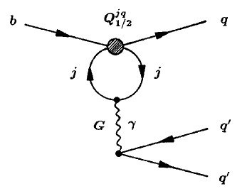
Figure 3: One-loop QCD and QED time-like penguin matrix elements of the current-current operators $Q_{1/2}^{jq}$.

Calculating both the one-loop QCD and QED time-like penguin matrix elements of the current-current operators $Q_{1/2}$ shown in Fig. 3, one finds^?,? the following non-vanishing elements $(\hat{m}_{s/e}(\mu))_{jk}$ ($j\in\{1,2\}$, $k\in\{3,\ldots,10\}$) of the matrices $\hat{m}_{s}(\mu)$ and $\hat{m}_{e}(\mu)$:

$$(\hat{m}_{s}(\mu))_{23} = (\hat{m}_{s}(\mu))_{25}=\,\,\,\,\,\frac{1}{6}\left[\frac{2}{3}\kappa+G(m,k,\mu)\right]$$

$$(\hat{m}_{s}(\mu))_{24} = (\hat{m}_{s}(\mu))_{26}=-\frac{1}{2}\left[\frac{2}{3}\kappa+G(m,k,\mu)\right]$$

$$(\hat{m}_{e}(\mu))_{17} = (\hat{m}_{e}(\mu))_{19}=-\frac{4}{3}\left[\frac{2}{3}\kappa+G(m,k,\mu)\right]$$ (24)

$$(\hat{m}_{e}(\mu))_{27} = (\hat{m}_{e}(\mu))_{29}=-\frac{4}{9}\left[\frac{2}{3}\kappa+G(m,k,\mu)\right]\,.$$

Here $\kappa$ parametrizes the renormalization scheme dependences and distinguishes between different mass-independent renormalization schemes. The function $G(m,k,\mu)$ is defined by

$$G(m,k,\mu)=-\,4\int\limits_{0}^{1}\mbox{d}x\,x\,(1-x)\ln\left[\frac{m^{2}-k^{2}\,x\,(1-x)}{\mu^{2}}\right],$$ (25)

where $m$ is the mass of the quark running in the loop of the penguin diagram shown in Fig. 3 and $k$ denotes the four-momentum of the virtual gluons and photons appearing in that figure.

The elements of the matrices $\hat{r}_{s}$ and $\hat{r}_{e}$ corresponding to (24) are given as follows^?-?:

$$(\hat{r}_{s})_{23} = (\hat{r}_{s})_{25}=\,\,\,\,\,\frac{1}{6}\left[\frac{2}{3}\kappa+\frac{10}{9}\right],\,\,\,(\hat{r}_{s})_{24}=(\hat{r}_{s})_{26}=-\frac{1}{2}\left[\frac{2}{3}\kappa+\frac{10}{9}\right]$$

$$(\hat{r}_{e})_{17} = (\hat{r}_{e})_{19}=-\frac{4}{3}\left[\frac{2}{3}\kappa+\frac{10}{9}\right],\,\,\,(\hat{r}_{e})_{27}=(\hat{r}_{e})_{29}=-\frac{4}{9}\left[\frac{2}{3}\kappa+\frac{10}{9}\right]\,.$$ (26)

Combining (2.3) with (24) and (26), we observe explicitly that the renormalization scheme dependent terms parametrized by $\kappa$ cancel each other and obtain the following renormalization scheme independent expression:

$$\left\langle\vec{Q}^{T}(\mu)\cdot\vec{C}(\mu)\right\rangle^{\mbox{{\scriptsize pen}}}=\sum\limits_{k=3}^{10}\langle Q_{k}\rangle_{0}\overline{C}_{k}(\mu)+\frac{\alpha_{s}(\mu)}{8\pi}\left[\frac{10}{9}-G(m,k,\mu)\right]$$ (27)

$$\times\Biggr{\{}\left(-\frac{1}{3}\langle Q_{3}\rangle_{0}+\langle Q_{4}\rangle_{0}-\frac{1}{3}\langle Q_{5}\rangle_{0}+\langle Q_{6}\rangle_{0}\right)\overline{C}_{2}(\mu)$$

$$+\frac{8}{9}\frac{\alpha}{\alpha_{s}(\mu)}\left(\langle Q_{7}\rangle_{0}+\langle Q_{9}\rangle_{0}\right)\left(3\overline{C}_{1}(\mu)+\overline{C}_{2}(\mu)\right)\Biggr{\}}\,.$$

The problems related to renormalization scheme dependences arising at NLO and their cancellation through certain matrix elements have also been investigated in Ref.^?. There additional subtleties, which are beyond the scope of this review, have been analyzed.

For later discussions it is useful to consider also the case where the proper renormalization group evolution from $\mu={\cal O}(M_{W})$ down to $\mu={\cal O}(m_{b})$ is neglected. The advantage of the corresponding Wilson coefficients is the point that they exhibit the top-quark mass dependence in a transparent way and allow moreover to investigate the importance of NLO renormalization group effects.

2.4 Neglect of the Proper Renormalization Group Evolution

If one does not perform the NLO renormalization group evolution from $\mu={\cal O}(M_{W})$ down to $\mu={\cal O}(m_{b})$ but calculates the relevant Feynman diagrams directly at a scale of ${\cal O}(M_{W})$ with full $W$ and $Z$ propagators and internal top-quark exchanges (see Fig. 2), one obtains the following set of coefficient functions^?:

$$\overline{C}^{(0)}_{1}(\mu) = {\cal O}(\alpha_{s}(\mu))+{\cal O}(\alpha),\quad\overline{C}^{(0)}_{2}(\mu)\,=\,1+{\cal O}(\alpha_{s}(\mu))+{\cal O}(\alpha)$$

$$\overline{C}^{(0)}_{3}(\mu) = -\frac{\alpha_{s}(\mu)}{24\pi}\left[E(x_{t})-\frac{\alpha}{\alpha_{s}(\mu)}\frac{1}{\sin^{2}\Theta_{\mbox{{\scriptsize W}}}}\left\{8B(x_{t})+4C(x_{t})\right\}+\frac{2}{3}\ln\frac{\mu^{2}}{M_{W}^{2}}-\frac{10}{9}\right]$$

$$\overline{C}^{(0)}_{4}(\mu) = -3\,\overline{C}^{(0)}_{5}(\mu)\,=\,\overline{C}^{(0)}_{6}(\mu)\,=\,\frac{\alpha_{s}(\mu)}{8\pi}\left[E(x_{t})+\frac{2}{3}\ln\frac{\mu^{2}}{M_{W}^{2}}-\frac{10}{9}\right]$$

$$\overline{C}^{(0)}_{7}(\mu) = \frac{\alpha}{6\pi}\left[4C(x_{t})+D(x_{t})+\frac{4}{9}\ln\frac{\mu^{2}}{M_{W}^{2}}-\frac{20}{27}\right]$$ (28)

$$\overline{C}^{(0)}_{8}(\mu) = \overline{C}^{(0)}_{10}(\mu)\,=\,0$$

$$\overline{C}^{(0)}_{9}(\mu) = \frac{\alpha}{6\pi}\left[4C(x_{t})+D(x_{t})+\frac{1}{\sin^{2}\Theta_{\mbox{{\scriptsize W}}}}\left\{10B(x_{t})-4C(x_{t})\right\}+\frac{4}{9}\ln\frac{\mu^{2}}{M_{W}^{2}}-\frac{20}{27}\right],$$

where $x_{t}\equiv m_{t}^{2}/M_{W}^{2}$ and

$$B(x)=\frac{1}{4}\left[\frac{x}{1-x}+\frac{x\ln x}{(x-1)^{2}}\right],\quad C(x)=\frac{x}{8}\left[\frac{x-6}{x-1}+\frac{3x+2}{(x-1)^{2}}\ln x\right],$$

$$D(x)=-\frac{4}{9}\ln x+\frac{-19x^{3}+25x^{2}}{36(x-1)^{3}}+\frac{x^{2}(5x^{2}-2x-6)}{18(x-1)^{4}}\ln x,$$ (29)

$$E(x)=-\frac{2}{3}\ln x+\frac{x(18-11x-x^{2})}{12(1-x)^{3}}+\frac{x^{2}(15-16x+4x^{2})}{6(1-x)^{4}}\ln x.$$

The Inami-Lim functions^? $B(x_{t})$, $C(x_{t})$, $D(x_{t})$ and $E(x_{t})$ describe contributions of box diagrams (which have not been shown in Fig. 2), $Z$ penguins, photon penguins and gluon penguins, respectively. Using the coefficients (28), QCD renormalization group effects are included only approximately through the rescaling $\alpha_{s}(M_{W})\to\alpha_{s}(\mu)$, where $\mu={\cal O}(m_{b})$. Note that the $\mu$-dependence of the coefficients $\overline{C}^{(0)}_{k}(\mu)$ originating from the logarithmic terms of the form $\ln(\mu^{2}/M_{W}^{2})$ is cancelled in the matrix element (27) by the one of the function $G(m,k,\mu)$. The ${\cal O}(\alpha_{s}(\mu))$ and ${\cal O}(\alpha)$ corrections to $\overline{C}^{(0)}_{1}(\mu)$ and $\overline{C}^{(0)}_{2}(\mu)$ contribute ${\cal O}(\alpha_{s}(\mu)^{2})$, ${\cal O}(\alpha\,\alpha_{s}(\mu))$ or ${\cal O}(\alpha^{2})$ effects to the penguin amplitude (27) and have to be neglected to the order we are working at in this review. For most practical applications, the differences between using the NLO Wilson coefficients or (28), i.e. the NLO renormalization group effects, are of order $(10-20)\%$ depending on the considered observables^?.

This remark concludes the brief introduction to low energy effective Hamiltonians calculated beyond LO. The subject of the subsequent section is a review of the current theoretical status of CP violation in non-leptonic $B$ decays and of strategies for extracting angles of the UT making use of these CP-violating effects.

3 CP Violation in Non-leptonic $B$-Meson Decays

Whereas CP-violating asymmetries in charged $B$ decays suffer in general from large hadronic uncertainties and are hence mainly interesting in respect of ruling out “superweak” models^? of CP violation, the neutral $B_{q}$-meson systems $(q\in\{d,s\})$ provide excellent laboratories to perform stringent tests of the SM description of CP violation^?. This feature is mainly due to “mixing-induced” CP violation which is absent in the charged $B$ system and arises from interference between decay- and $B^{0}_{q}-\overline{B^{0}_{q}}$ mixing-processes. In order to derive the formulae for the corresponding CP-violating asymmetries, we have to discuss $B^{0}_{q}-\overline{B^{0}_{q}}$ mixing first.

3.1 The Phenomenon of $B^{0}_{q}-\overline{B^{0}_{q}}$ Mixing

Within the SM, $B^{0}_{q}-\overline{B^{0}_{q}}$ mixing is induced at lowest order through the box diagrams shown in Fig. 4. Applying a matrix notation, the Wigner-Weisskopf formalism^? yields an effective Schrödinger equation of the form

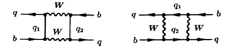
Figure 4: Box diagrams contributing to $B^{0}_{q}-\overline{B^{0}_{q}}$ mixing $(q_{1},q_{2}\in\{u,c,t\})$.

$$i\,\frac{\partial}{\partial t}\left(\begin{array}[]{c}a(t)\\ b(t)\end{array}\right)=\left[\left(\begin{array}[]{cc}M_{0}^{(q)}&M_{12}^{(q)}\\ M_{12}^{(q)\ast}&M_{0}^{(q)}\end{array}\right)-\frac{i}{2}\left(\begin{array}[]{cc}\Gamma_{0}^{(q)}&\Gamma_{12}^{(q)}\\ \Gamma_{12}^{(q)\ast}&\Gamma_{0}^{(q)}\end{array}\right)\right]\cdot\left(\begin{array}[]{c}a(t)\\ b(t)\end{array}\right)$$ (30)

describing the time evolution of the state vector

$$\left|\psi_{q}(t)\right\rangle=a(t)\left|B^{0}_{q}\right\rangle+b(t)\left|\overline{B^{0}_{q}}\right\rangle.$$ (31)

The special form of the mass and decay matrices in (30) follows from invariance under CPT transformations. It is an easy exercise to evaluate the eigenstates $\left|B_{\pm}^{(q)}\right\rangle$ with eigenvalues $\lambda_{\pm}^{(q)}$ of that Hamilton operator. They are given by

$$\left|B_{\pm}^{(q)}\right\rangle=\frac{1}{\sqrt{1+|\alpha_{q}|^{2}}}\left(\left|B^{0}_{q}\right\rangle\pm\alpha_{q}\left|\overline{B^{0}_{q}}\right\rangle\right)$$ (32)

$$\lambda_{\pm}^{(q)}=\left(M_{0}^{(q)}-\frac{i}{2}\Gamma_{0}^{(q)}\right)\pm\left(M_{12}^{(q)}-\frac{i}{2}\Gamma_{12}^{(q)}\right)\alpha_{q},$$ (33)

where

$$\alpha_{q}=\sqrt{\frac{4|M_{12}^{(q)}|^{2}e^{-i2\delta\Theta_{M/\Gamma}^{(q)}}+|\Gamma_{12}^{(q)}|^{2}}{4|M_{12}^{(q)}|^{2}+|\Gamma_{12}^{(q)}|^{2}-4|M_{12}^{(q)}||\Gamma_{12}^{(q)}|\sin\delta\Theta_{M/\Gamma}^{(q)}}}e^{-i\left(\Theta_{\Gamma_{12}}^{(q)}+n^{\prime}\pi\right)}.$$ (34)

Here the notations $M_{12}^{(q)}\equiv e^{i\Theta_{M_{12}}^{(q)}}|M_{12}^{(q)}|$, $\Gamma_{12}^{(q)}\equiv e^{i\Theta_{\Gamma_{12}}^{(q)}}|\Gamma_{12}^{(q)}|$ and $\delta\Theta_{M/\Gamma}^{(q)}\equiv\Theta_{M_{12}}^{(q)}-\Theta_{\Gamma_{12}}^{(q)}$ have been introduced and $n^{\prime}\in{\rm Z}$ parametrizes the sign of the square root appearing in that expression. Calculating the dispersive and absorptive parts of the box diagrams depicted in Fig. 4 one obtains^?

$$M_{12}^{(q)} = \frac{G_{\mbox{{\scriptsize F}}}^{2}M_{W}^{2}M_{B_{q}}B_{B_{q}}f_{B_{q}}^{2}}{12\pi^{2}}$$

$$\times\left[v_{c}^{(q)2}S(x_{c})+v_{t}^{(q)2}S(x_{t})+2v_{c}^{(q)}v_{t}^{(q)}S(x_{c},x_{t})\right]e^{i(\pi-\phi_{\mbox{{\scriptsize CP}}}(B_{q}))}$$

and

$$\Gamma_{12}^{(q)}=\frac{G_{\mbox{{\scriptsize F}}}^{2}m_{b}^{2}M_{B_{q}}B_{B_{q}}f_{B_{q}}^{2}}{8\pi}\left[v_{t}^{(q)2}+\frac{8}{3}v_{c}^{(q)}v_{t}^{(q)}\left(z_{c}+\frac{1}{4}z_{c}^{2}-\frac{1}{2}z_{c}^{3}\right)\right.$$

$$+\left.v_{c}^{(q)2}\left\{\sqrt{1-4z_{c}}\left(1-\frac{2}{3}z_{c}\right)+\frac{8}{3}z_{c}+\frac{2}{3}z_{c}^{2}-\frac{4}{3}z_{c}^{3}-1\right\}\right]e^{-i\phi_{\mbox{{\scriptsize CP}}}(B_{q})},$$

respectively, where $x_{c}\equiv m_{c}^{2}/M_{W}^{2}$, $x_{t}\equiv m_{t}^{2}/M_{W}^{2}$, $z_{c}\equiv m_{c}^{2}/m_{b}^{2}$ and $v_{i}^{(q)}\equiv V_{iq}^{\ast}V_{ib}$. The non-perturbative “$B$-parameter” $B_{B_{q}}={\cal O}(1)$ is related to the hadronic matrix element $\bigl{\langle}\overline{B^{0}_{q}}\bigl{|}[\bar{b}\gamma_{\mu}(1-\gamma_{5})q]^{2}\bigr{|}B_{q}^{0}\bigr{\rangle}$, $f_{B_{q}}$ is the $B_{q}$-meson decay constant and $M_{B_{q}}$ denotes the mass of the $B_{q}$-meson. The functions $S(x)$ and $S(x,y)$ are given by

$$S(x)=\left[\frac{1}{4}-\frac{9}{4(x-1)}-\frac{3}{2(x-1)^{2}}\right]x+\frac{3}{2}\left(\frac{x}{x-1}\right)^{3}\ln{x}$$ (37)

$$S(x,y)=\frac{xy}{x-y}\left[\frac{1}{4}-\frac{3}{2(x-1)}-\frac{3}{4(x-1)^{2}}\right]\ln x+(x\leftrightarrow y)-\frac{3xy}{4(x-1)(y-1)}$$ (38)

and the phase $\phi_{\mbox{{\scriptsize CP}}}(B_{q})$ parametrizing the applied CP phase convention is defined through

$$({\cal CP})\left|B^{0}_{q}\right\rangle=e^{i\phi_{\mbox{{\scriptsize CP}}}(B_{q})}\left|\overline{B^{0}_{q}}\right\rangle.$$ (39)

In the presence of a heavy top-quark of mass $m_{t}={\cal O}(170\,\mbox{GeV})$ we have $S(x_{t})={\cal O}(1)$, $S(x_{c})={\cal O}(10^{-4})$ and $S(x_{c},x_{t})={\cal O}(10^{-3})$. Consequently, since $v_{c}^{(q)}$ and $v_{t}^{(q)}$ are of the same order in $\lambda$ (${\cal O}(\lambda^{3})$ and ${\cal O}(\lambda^{2})$ for $q=d$ and $s$, respectively), $M_{12}^{(q)}$ is governed by internal top-quark exchanges and can be approximated as

$$M_{12}^{(q)}=\frac{G_{\mbox{{\scriptsize F}}}^{2}M_{W}^{2}M_{B_{q}}B_{B_{q}}f_{B_{q}}^{2}}{12\pi^{2}}\,v_{t}^{(q)2}S(x_{t})\,e^{i\left(\pi-\phi_{\mbox{{\scriptsize CP}}}(B_{q})\right)}.$$ (40)

On the other hand, since the expression (3.1) for the off-diagonal element $\Gamma_{12}^{(q)}$ of the decay matrix is dominated by the term proportional to $v_{t}^{(q)2}$, we have

$$\frac{\Gamma_{12}^{(q)}}{M_{12}^{(q)}}\approx-\frac{3\pi}{2S(x_{t})}\frac{m_{b}^{2}}{M_{W}^{2}}.$$ (41)

Therefore, $|\Gamma_{12}^{(q)}|/|M_{12}^{(q)}|={\cal O}(m_{b}^{2}/m_{t}^{2})\ll 1$. Expanding (34) in powers of this small quantity gives

$$\alpha_{q}=\left[1+\frac{|\Gamma_{12}^{(q)}|}{2|M_{12}^{(q)}|}\sin\delta\Theta_{M/\Gamma}^{(q)}\right]e^{-i\left(\Theta_{M_{12}}^{(q)}+n^{\prime}\pi\right)}+{\cal O}\left(\left(\frac{|\Gamma_{12}^{(q)}|}{|M_{12}^{(q)}|}\right)^{2}\right).$$ (42)

The deviation of $|\alpha_{q}|$ from 1 describes CP-violating effects in $B^{0}_{q}-\overline{B^{0}_{q}}$ oscillations. This type of CP violation is probed by rate asymmetries in semileptonic decays of neutral $B_{q}$-mesons into “wrong charge” leptons, i.e. by comparing the rate of an initially pure $B_{q}^{0}$-meson decaying into $l^{-}\overline{\nu}_{l}X$ with that of an initially pure $\overline{B^{0}_{q}}$ decaying into $l^{+}\nu_{l}X$:

$${\cal A}^{(q)}_{\mbox{{\scriptsize SL}}}\equiv\frac{\Gamma(B^{0}_{q}(t)\to l^{-}\overline{\nu}_{l}X)-\Gamma(\overline{B^{0}_{q}}(t)\to l^{+}\nu_{l}X)}{\Gamma(B^{0}_{q}(t)\to l^{-}\overline{\nu}_{l}X)+\Gamma(\overline{B^{0}_{q}}(t)\to l^{+}\nu_{l}X)}=\frac{|\alpha_{q}|^{4}-1}{|\alpha_{q}|^{4}+1}\approx\frac{|\Gamma_{12}^{(q)}|}{|M_{12}^{(q)}|}\sin\delta\Theta^{(q)}_{M/\Gamma}.$$ (43)

Note that the time dependences cancel in (43). Because of $|\Gamma_{12}^{(q)}|/|M_{12}^{(q)}|\propto m_{b}^{2}/m_{t}^{2}$ and $\sin\delta\Theta^{(q)}_{M/\Gamma}\propto m_{c}^{2}/m_{b}^{2}$, the asymmetry (43) is suppressed by a factor $m_{c}^{2}/m_{t}^{2}={\cal O}(10^{-4})$ and is hence expected to be very small within the SM. At present there exists an experimental upper bound $|\mbox{Re}(\varepsilon_{B_{d}})|\equiv|{\cal A}^{(d)}_{\mbox{{\scriptsize SL}}}/4|<45\cdot 10^{-3}$ (90% C.L.) from the CLEO collaboration^? which is about two orders of magnitudes above the SM prediction.

The time-evolution of initially, i.e. at $t=0$, pure $\left|B^{0}_{q}\right\rangle$ and $\left|\overline{B^{0}_{q}}\right\rangle$ meson states is given by

$$\left|B^{0}_{q}(t)\right\rangle = f_{+}^{(q)}(t)\left|B^{0}_{q}\right\rangle+\alpha_{q}f_{-}^{(q)}(t)\left|\overline{B^{0}_{q}}\right\rangle$$ (44)

$$\left|\overline{B^{0}_{q}}(t)\right\rangle = \frac{1}{\alpha_{q}}f_{-}^{(q)}(t)\left|B^{0}_{q}\right\rangle+f_{+}^{(q)}(t)\left|\overline{B^{0}_{q}}\right\rangle,$$ (45)

where

$$f_{\pm}^{(q)}(t)=\frac{1}{2}\left(e^{-i\lambda_{+}^{(q)}t}\pm e^{-i\lambda_{-}^{(q)}t}\right).$$ (46)

Using these time-dependent state vectors and neglecting the very small CP-violating effects in $B^{0}_{q}-\overline{B^{0}_{q}}$ mixing that are described by $|\alpha_{q}|\not=1$ (see (42)), a straightforward calculation yields^?

$$\Gamma(B^{0}_{q}(t)\to f) = \left[\left|g_{+}^{(q)}(t)\right|^{2}+\left|\xi_{f}^{(q)}\right|^{2}\left|g_{-}^{(q)}(t)\right|^{2}-2\mbox{\,Re}\left\{\xi_{f}^{(q)}g_{-}^{(q)}(t)g_{+}^{(q)}(t)^{\ast}\right\}\right]\tilde{\Gamma}$$ (47)

$$\Gamma(\overline{B^{0}_{q}}(t)\to f) = \left[\left|g_{-}^{(q)}(t)\right|^{2}+\left|\xi_{f}^{(q)}\right|^{2}\left|g_{+}^{(q)}(t)\right|^{2}-2\mbox{\,Re}\left\{\xi_{f}^{(q)}g_{+}^{(q)}(t)g_{-}^{(q)}(t)^{\ast}\right\}\right]\tilde{\Gamma}\quad$$ (48)

$$\Gamma(B^{0}_{q}(t)\to\overline{f}) = \left[\left|g_{+}^{(q)}(t)\right|^{2}+\left|\xi_{\overline{f}}^{(q)}\right|^{2}\left|g_{-}^{(q)}(t)\right|^{2}-2\mbox{\,Re}\left\{\xi_{\overline{f}}^{(q)}g_{-}^{(q)}(t)g_{+}^{(q)}(t)^{\ast}\right\}\right]\tilde{\overline{\Gamma}}$$ (49)

$$\Gamma(\overline{B^{0}_{q}}(t)\to\overline{f}) = \left[\left|g_{-}^{(q)}(t)\right|^{2}+\left|\xi_{\overline{f}}^{(q)}\right|^{2}\left|g_{+}^{(q)}(t)\right|^{2}-2\mbox{\,Re}\left\{\xi_{\overline{f}}^{(q)}g_{+}^{(q)}(t)g_{-}^{(q)}(t)^{\ast}\right\}\right]\tilde{\overline{\Gamma}},$$ (50)

where

$$\left|g^{(q)}_{\pm}(t)\right|^{2}=\frac{1}{4}\left[e^{-\Gamma_{L}^{(q)}t}+e^{-\Gamma_{H}^{(q)}t}\pm 2\,e^{-\Gamma_{q}t}\cos(\Delta M_{q}t)\right]$$ (51)

$$g_{-}^{(q)}(t)\,g_{+}^{(q)}(t)^{\ast}=\frac{1}{4}\left[e^{-\Gamma_{L}^{(q)}t}-e^{-\Gamma_{H}^{(q)}t}+2\,i\,e^{-\Gamma_{q}t}\sin(\Delta M_{q}t)\right]$$ (52)

and

$$\xi_{f}^{(q)}=e^{-i\Theta_{M_{12}}^{(q)}}\frac{A(\overline{B_{q}^{0}}\to f)}{A(B_{q}^{0}\to f)},\quad\xi_{\overline{f}}^{(q)}=e^{-i\Theta_{M_{12}}^{(q)}}\frac{A(\overline{B_{q}^{0}}\to\overline{f})}{A(B_{q}^{0}\to\overline{f})}.$$ (53)

In the time-dependent rates (47)-(50), the time-independent transition rates $\tilde{\Gamma}$ and $\tilde{\overline{\Gamma}}$ correspond to the “unevolved” decay amplitudes $A(B^{0}_{q}\to f)$ and $A(B^{0}_{q}\to\overline{f})$, respectively, and can be calculated by performing the usual phase space integrations. The functions $g_{\pm}^{(q)}(t)$ are related to $f_{\pm}^{(q)}(t)$. However, whereas the latter functions depend through $\alpha_{q}$ on the quantity $n^{\prime}$ parametrizing the sign of the square root appearing in (34), $g_{\pm}^{(q)}(t)$ and the rates (47)-(50) do not depend on that parameter. The $n^{\prime}$-dependence is cancelled by introducing the positive mass difference

$$\Delta M_{q}\equiv M_{H}^{(q)}-M_{L}^{(q)}=2\left|M_{12}^{(q)}\right|>0$$ (54)

of the $B_{q}$ mass eigenstates, where $H$ and $L$ refer to “heavy” and “light”, respectively. The quantities $\Gamma_{H}^{(q)}$ and $\Gamma_{L}^{(q)}$ denote the corresponding decay widths. Their difference can be expressed as

$$\Delta\Gamma_{q}\equiv\Gamma_{H}^{(q)}-\Gamma_{L}^{(q)}=\frac{4\mbox{\,Re}\left[M_{12}^{(q)}\Gamma_{12}^{(q)\ast}\right]}{\Delta M_{q}},$$ (55)

while the average decay width of the $B_{q}$ mass eigenstates is given by

$$\Gamma_{q}\equiv\frac{\Gamma^{(q)}_{H}+\Gamma^{(q)}_{L}}{2}=\Gamma^{(q)}_{0}.$$ (56)

Whereas both the mixing phase $\Theta_{M_{12}}^{(q)}$ and the amplitude ratios appearing in (53) depend on the chosen CP phase convention parametrized through $\phi_{\mbox{{\scriptsize CP}}}(B_{q})$, the quantities $\xi_{f}^{(q)}$ and $\xi_{\overline{f}}^{(q)}$ are convention independent observables. We shall see the cancellation of $\phi_{\mbox{{\scriptsize CP}}}(B_{q})$ explicitly in a moment.

The $B^{0}_{q}-\overline{B^{0}_{q}}$ mixing phase $\Theta_{M_{12}}^{(q)}$ appearing in the equations given above is essential for the later discussion of “mixing-induced” CP violation. As can be read off from the expression (40) for the off-diagonal element $M_{12}^{(q)}$ of the mass matrix, $\Theta_{M_{12}}^{(q)}$ is related to complex phases of CKM matrix elements through

$$\Theta_{M_{12}}^{(q)}=\pi+2\,\mbox{arg}\left(V_{tq}^{\ast}V_{tb}\right)-\phi_{\mbox{{\scriptsize CP}}}(B_{q}).$$ (57)

In (40), perturbative QCD corrections to $B^{0}_{q}-\overline{B^{0}_{q}}$ mixing have been neglected. Since these corrections, which are presently known up to NLO^?, show up as a factor $\eta_{\mbox{{\scriptsize QCD}}}\approx 0.55$ multiplying the r.h.s. of (40), they do not affect the mixing phase $\Theta_{M_{12}}^{(q)}$ and have therefore no significance for mixing-induced CP violation.

A measure of the strength of the $B^{0}_{q}-\overline{B^{0}_{q}}$ oscillations is provided by the “mixing parameter”

$$x_{q}\equiv\frac{\Delta M_{q}}{\Gamma_{q}}.$$ (58)

The present ranges for $x_{d}$ and $x_{s}$ can be summarized as

$$x_{q}=\left\{\begin{array}[]{ll}0.72\pm 0.03&\mbox{\quad for $q=d$}\\ \quad{\cal O}(20)&\mbox{\quad for $q=s$,}\end{array}\right.$$ (59)

where $1/\Gamma_{d}=1.55\,\mbox{ps}$ has been used to evaluate $x_{d}$ from the present experimental values for $\Delta M_{d}$ summarized recently in Ref.^?. So far the mixing parameter $x_{s}$ has not been measured directly and only an experimental lower bound $x_{s}\cdot\Gamma_{s}=\Delta M_{s}>9.2/\mbox{ps}$, which is based in particular on recent ALEPH and DELPHI results^?, is available. Within the SM one expects^? $x_{s}$ to be of ${\cal O}(20)$. That information can be obtained with the help of the relation

$$x_{s}=x_{d}\,\frac{1}{|V_{us}|^{2}R_{t}^{2}}\,\frac{1}{R_{ds}}\quad\mbox{with}\quad R_{ds}=\frac{\Gamma_{s}}{\Gamma_{d}}\cdot\frac{M_{B_{d}}}{M_{B_{s}}}\left[\frac{f_{B_{d}}\sqrt{B_{B_{d}}}}{f_{B_{s}}\sqrt{B_{B_{s}}}}\right]^{2},$$ (60)

where $R_{ds}$ describes $SU(3)$ flavor-breaking effects. Note that $R_{ds}=1$ in the strict $SU(3)$ limit.

The mixing parameters listed in (59) have interesting phenomenological consequences for the width differences $\Delta\Gamma_{d,s}$ defined by (55). Using this expression we obtain

$$\frac{\Delta\Gamma_{q}}{\Gamma_{q}}\approx-\frac{3\pi}{2S(x_{t})}\frac{m_{b}^{2}}{M_{W}^{2}}\,x_{q}.$$ (61)

Consequently $\Delta\Gamma_{q}$ is negative so that the decay width $\Gamma_{H}^{(q)}$ of the “heavy” mixing eigenstate is smaller than that of the “light” eigenstate. Since the numerical factor in (61) multiplying the mixing parameter $x_{q}$ is ${\cal O}(10^{-2})$, the width difference $\Delta\Gamma_{d}$ is very small within the SM. On the other hand, the expected large value of $x_{s}$ implies a sizable $\Delta\Gamma_{s}$ which may be as large as ${\cal O}(20\%)$. The dynamical origin of this width difference is related to CKM favored $\bar{b}\to\bar{c}c\bar{s}$ quark-level transitions into final states that are common both to $B^{0}_{s}$ and $\overline{B^{0}_{s}}$ mesons. Theoretical analyses of $\Delta\Gamma_{s}/\Gamma_{s}$ indicate that it may indeed be as large as ${\cal O}(20\%)$. These studies are based on box diagram calculations^?, on a complementary approach^? where one sums over many exclusive $\bar{b}\to\bar{c}c\bar{s}$ modes, and on the Heavy Quark Expansion yielding the most recent result^? $\Delta\Gamma_{s}/\Gamma_{s}=0.16^{+0.11}_{-0.09}$. This width difference can be determined experimentally e.g. from angular correlations in $B_{s}\to J/\psi\,\phi$ decays^?. One expects $10^{3}-10^{4}$ reconstructed $B_{s}\to J/\psi\,\phi$ events both at Tevatron Run II and at HERA-B which may allow a precise measurement of $\Delta\Gamma_{s}$. As was pointed out by Dunietz^?, $\Delta\Gamma_{s}$ may lead to interesting CP-violating effects in untagged data samples of time-evolved $B_{s}$ decays where one does not distinguish between initially present $B^{0}_{s}$ and $\overline{B^{0}_{s}}$ mesons. Before we shall turn to detailed discussions of CP-violating asymmetries in the $B_{d}$ system and of the $B_{s}$ system in light of $\Delta\Gamma_{s}$, let us focus on $B_{q}$ decays ($q\in\{d,s\}$) into final CP eigenstates first. For an analysis of transitions into non CP eigenstates the reader is referred to Ref.^?.

3.2 $B_{q}$ Decays into CP Eigenstates

A very promising special case in respect of extracting CKM phases from CP-violating effects in neutral $B_{q}$ decays are transitions into final states $|f\rangle$ that are eigenstates of the CP operator and hence satisfy

$$({\cal CP})|f\rangle=\pm|f\rangle.$$ (62)

Consequently we have $\xi_{f}^{(q)}=\xi_{\overline{f}}^{(q)}$ in that case (see (53)) and have to deal only with a single observable $\xi_{f}^{(q)}$ containing essentially all the information that is needed to evaluate the time-dependent decay rates (47)-(50). Decays into final states that are not eigenstates of the CP operator play an important role in the case of the $B_{s}$ system to extract the UT angle $\gamma$ and are discussed in 3.4.5.

3.2.1 Calculation of $\xi_{f}^{(q)}$

Whereas the $B^{0}_{q}-\overline{B^{0}_{q}}$ mixing phase $\Theta_{M_{12}}^{(q)}$ entering the expression (53) for $\xi_{f}^{(q)}$ is simply given as a function of complex phases of certain CKM matrix elements (see (57)), the amplitude ratio $A(\overline{B^{0}_{q}}\to f)/A(B^{0}_{q}\to f)$ requires the calculation of hadronic matrix elements which are poorly known at present. In order to investigate this amplitude ratio, we shall employ the low energy effective Hamiltonian for $|\Delta B|=1$, $\Delta C=\Delta U=0$ transitions discussed in Section 2. Using (15) we get

$$A\left(\overline{B^{0}_{q}}\to f\right)=\Bigl{\langle}f\Bigl{|}{\cal H}_{\mbox{{\scriptsize eff}}}(\Delta B=-1)\Bigr{|}\overline{B^{0}_{q}}\Bigr{\rangle}$$

$$=\Biggl{\langle}f\left|\frac{G_{\mbox{{\scriptsize F}}}}{\sqrt{2}}\left[\sum\limits_{j=u,c}V_{jr}^{\ast}V_{jb}\left\{\sum\limits_{k=1}^{2}Q_{k}^{jr}(\mu)C_{k}(\mu)+\sum\limits_{k=3}^{10}Q_{k}^{r}(\mu)C_{k}(\mu)\right\}\right]\right|\overline{B^{0}_{q}}\Biggr{\rangle},$$

where the flavor label $r\in\{d,s\}$ distinguishes – as in the whole subsection – between $b\to d$ and $b\to s$ transitions. On the other hand, the transition amplitude $A\left(B^{0}_{q}\to f\right)$ is given by

$$A\left(B^{0}_{q}\to f\right)=\left\langle f\left|{\cal H}_{\mbox{{\scriptsize eff}}}(\Delta B=-1)^{\dagger}\right|B^{0}_{q}\right\rangle$$

$$=\Biggl{\langle}f\left|\frac{G_{\mbox{{\scriptsize F}}}}{\sqrt{2}}\left[\sum\limits_{j=u,c}V_{jr}V_{jb}^{\ast}\left\{\sum\limits_{k=1}^{2}Q_{k}^{jr\dagger}(\mu)C_{k}(\mu)+\sum\limits_{k=3}^{10}Q_{k}^{r\dagger}(\mu)C_{k}(\mu)\right\}\right]\right|B^{0}_{q}\Biggr{\rangle}.$$

Performing appropriate CP transformations in this equation, i.e. inserting the operator $({\cal CP})^{\dagger}({\cal CP})=\hat{1}$ both after the bra $\langle f|$ and in front of the ket $|B^{0}_{q}\rangle$, yields

$$A\left(B^{0}_{q}\to f\right)=\pm e^{i\phi_{\mbox{{\scriptsize CP}}}(B_{q})}$$

$$\times\Biggl{\langle}f\left|\frac{G_{\mbox{{\scriptsize F}}}}{\sqrt{2}}\left[\sum\limits_{j=u,c}V_{jr}V_{jb}^{\ast}\left\{\sum\limits_{k=1}^{2}Q_{k}^{jr}(\mu)C_{k}(\mu)+\sum\limits_{k=3}^{10}Q_{k}^{r}(\mu)C_{k}(\mu)\right\}\right]\right|\overline{B^{0}_{q}}\Biggr{\rangle},$$

where we have applied the relation

$$({\cal CP})Q_{k}^{jr\dagger}({\cal CP})^{\dagger}=Q_{k}^{jr}$$ (66)

and have furthermore taken into account (39) and (62). Consequently we obtain

$$\frac{A(\overline{B^{0}_{q}}\to f)}{A(B^{0}_{q}\to f)}=\pm\,e^{-i\phi_{\mbox{{\scriptsize CP}}}(B_{q})}\,\frac{\sum\limits_{j=u,c}v_{j}^{(r)}\Bigl{\langle}f\Bigl{|}{\cal Q}^{jr}\Bigr{|}\overline{B^{0}_{q}}\Bigr{\rangle}}{\sum\limits_{j=u,c}v_{j}^{(r)\ast}\Bigl{\langle}f\Bigl{|}{\cal Q}^{jr}\Bigr{|}\overline{B^{0}_{q}}\Bigr{\rangle}},$$ (67)

where $v_{j}^{(r)}\equiv V_{jr}^{\ast}V_{jb}$ and the operators ${\cal Q}^{jr}$ are defined by

$${\cal Q}^{jr}\equiv\sum\limits_{k=1}^{2}Q_{k}^{jr}C_{k}(\mu)+\sum\limits_{k=3}^{10}Q_{k}^{r}C_{k}(\mu).$$ (68)

Inserting (57) and (67) into the expression (53) for $\xi_{f}^{(q)}$, we observe explicitly that the convention dependent phases $\phi_{\mbox{{\scriptsize CP}}}(B_{q})$ appearing in the former two equations cancel each other and arrive at the convention independent result

$$\xi_{f}^{(q)}=\mp\,e^{-i\phi_{\mbox{{\scriptsize M}}}^{(q)}}\frac{\sum\limits_{j=u,c}v_{j}^{(r)}\Bigl{\langle}f\Bigl{|}{\cal Q}^{jr}\Bigr{|}\overline{B^{0}_{q}}\Bigr{\rangle}}{\sum\limits_{j=u,c}v_{j}^{(r)\ast}\Bigl{\langle}f\Bigl{|}{\cal Q}^{jr}\Bigr{|}\overline{B^{0}_{q}}\Bigr{\rangle}}.$$ (69)

Here the phase $\phi_{\mbox{{\scriptsize M}}}^{(q)}\equiv 2\,\mbox{arg}(V_{tq}^{\ast}V_{tb})$ arises from the $B^{0}_{q}-\overline{B^{0}_{q}}$ mixing phase $\Theta_{M_{12}}^{(q)}$. Applying the modified Wolfenstein parametrization (10), $\phi_{\mbox{{\scriptsize M}}}^{(q)}$ can be related to angles of the UT as follows:

$$\phi_{\mbox{{\scriptsize M}}}^{(q)}=\left\{\begin{array}[]{cl}2\beta&\mbox{for $q=d$}\\ 0&\mbox{for $q=s$.}\end{array}\right.$$ (70)

Consequently a non-trivial mixing phase arises only in the $B_{d}$ system.

In general the observable $\xi_{f}^{(q)}$ suffers from large hadronic uncertainties that are introduced through the hadronic matrix elements appearing in (69). However, there is a very important special case where these uncertainties cancel and theoretical clean predictions of $\xi_{f}^{(q)}$ are possible.

3.2.2 Dominance of a Single CKM Amplitude

If the transition matrix elements appearing in (69) are dominated by a single CKM amplitude, the observable $\xi_{f}^{(q)}$ takes the very simple form

$$\xi_{f}^{(q)}=\mp\exp\left[-i\left\{\phi_{\mbox{{\scriptsize M}}}^{(q)}-\phi_{\mbox{{\scriptsize D}}}^{(f)}\right\}\right],$$ (71)

where the characteristic “decay” phase $\phi_{\mbox{{\scriptsize D}}}^{(f)}$ can be expressed in terms of angles of the UT as follows:

$$\phi_{\mbox{{\scriptsize D}}}^{(f)}=\left\{\begin{array}[]{cl}-2\gamma&\mbox{for dominant $\bar{b}\to\bar{u}u\bar{r}$ CKM amplitudes in $B_{q}^{0}\to f$}\\ 0&\mbox{for dominant $\bar{b}\to\bar{c}c\bar{r}$\,\, CKM amplitudes in $B_{q}^{0}\to f$.}\end{array}\right.$$ (72)

The validity of dominance of a single CKM amplitude and important phenomenological applications of (71) will be discussed in the following subsections.

3.3 The $B_{d}$ System

In contrast to the $B_{s}$ system, the width difference is negligibly small in the $B_{d}$ system. Consequently the expressions for the decay rates (47)-(50) simplify considerably in that case.

3.3.1 CP Asymmetries in $B_{d}$ Decays

Restricting ourselves, as in the previous subsection, to decays into final CP eigenstates $|f\rangle$ satisfying (62), we obtain the following expressions for the time-dependent and time-integrated CP asymmetries:

$$a_{\mbox{{\scriptsize CP}}}(B_{d}\to f;t)\equiv\frac{\Gamma(B_{d}^{0}(t)\to f)-\Gamma(\overline{B_{d}^{0}}(t)\to f)}{\Gamma(B_{d}^{0}(t)\to f)+\Gamma(\overline{B_{d}^{0}}(t)\to f)}$$ (73)

$$={\cal A}_{\mbox{{\scriptsize CP}}}^{\mbox{{\scriptsize dir}}}(B_{d}\to f)\cos(\Delta M_{d}t)+{\cal A}_{\mbox{{\scriptsize CP}}}^{\mbox{{\scriptsize mix-ind}}}(B_{d}\to f)\sin(\Delta M_{d}t)$$

$$a_{\mbox{{\scriptsize CP}}}(B_{d}\to f)\equiv\frac{\int\limits_{0}^{\infty}\mbox{d}t\left[\Gamma(B_{d}^{0}(t)\to f)-\Gamma(\overline{B_{d}^{0}}(t)\to f)\right]}{\int\limits_{0}^{\infty}\mbox{d}t\left[\Gamma(B_{d}^{0}(t)\to f)+\Gamma(\overline{B_{d}^{0}}(t)\to f)\right]}$$ (74)

$$=\frac{1}{1+x_{d}^{2}}\left[{\cal A}_{\mbox{{\scriptsize CP}}}^{\mbox{{\scriptsize dir}}}(B_{d}\to f)+x_{d}\,{\cal A}_{\mbox{{\scriptsize CP}}}^{\mbox{{\scriptsize mix-ind}}}(B_{d}\to f)\right],$$

where the direct CP-violating contributions

$${\cal A}_{\mbox{{\scriptsize CP}}}^{\mbox{{\scriptsize dir}}}(B_{d}\to f)\equiv\frac{1-\left|\xi_{f}^{(d)}\right|^{2}}{1+\left|\xi_{f}^{(d)}\right|^{2}}$$ (75)

have been separated from the mixing-induced CP-violating contributions

$${\cal A}_{\mbox{{\scriptsize CP}}}^{\mbox{{\scriptsize mix-ind}}}(B_{d}\to f)\equiv\frac{2\,\mbox{Im}\,\xi_{f}^{(d)}}{1+\left|\xi_{f}^{(d)}\right|^{2}}.$$ (76)

Whereas the former observables describe CP violation arising directly in the corresponding decay amplitudes, the latter ones are due to interference between $B^{0}_{d}-\overline{B^{0}_{d}}$ mixing- and decay-processes. Needless to say, the expressions (73) and (74) have to be modified appropriately for the $B_{s}$ system because of $\Delta\Gamma_{s}/\Gamma_{s}={\cal O}(20\%)$. In the case of the time-dependent CP asymmetry (73) these effects start to become important for $t\,\mbox{{\scriptsize$\stackrel{{\scriptstyle>}}{{\sim}}$}}\,2/\Delta\Gamma_{s}$.

3.3.2 CP Violation in $B_{d}\to J/\psi\,K_{\mbox{{\scriptsize S}}}$: the “Gold-plated” Way to Extract $\beta$

The channel $B_{d}\to J/\psi\,K_{\mbox{{\scriptsize S}}}$ is a transition into a CP eigenstate with eigenvalue $-1$ and originates from a $\bar{b}\to\bar{c}c\bar{s}$ quark-level decay^?. Consequently the corresponding observable $\xi^{(d)}_{\psi K_{\mbox{{\scriptsize S}}}}$ can be expressed as

$$\xi^{(d)}_{\psi K_{\mbox{{\scriptsize S}}}}=+e^{-2i\beta}\left[\frac{v_{u}^{(s)}A^{ut^{\prime}}_{\mbox{{\scriptsize pen}}}+v_{c}^{(s)}\left(A_{\mbox{{\scriptsize cc}}}^{c^{\prime}}+A^{ct^{\prime}}_{\mbox{{\scriptsize pen}}}\right)}{v_{u}^{(s)\ast}A^{ut^{\prime}}_{\mbox{{\scriptsize pen}}}+v_{c}^{(s)\ast}\left(A_{\mbox{{\scriptsize cc}}}^{c^{\prime}}+A^{ct^{\prime}}_{\mbox{{\scriptsize pen}}}\right)}\right],$$ (77)

where $A_{\mbox{{\scriptsize cc}}}^{c^{\prime}}$ denotes the $Q_{1/2}^{cs}$ current-current operator amplitude and $A^{ut^{\prime}}_{\mbox{{\scriptsize pen}}}$ $(A^{ct^{\prime}}_{\mbox{{\scriptsize pen}}})$ corresponds to contributions of the penguin-type with up- and top-quarks (charm- and top-quarks) running as virtual particles in the loops. Note that within this notation penguin-like matrix elements of the $Q_{1/2}^{cs}$ operators like those depicted in Fig. 3 are included by definition in the $A^{ct^{\prime}}_{\mbox{{\scriptsize pen}}}$ amplitude, whereas those of $Q_{1/2}^{us}$ show up in $A^{ut^{\prime}}_{\mbox{{\scriptsize pen}}}$. The primes in (77) have been introduced to remind us that we are dealing with a $\bar{b}\to\bar{s}$ mode. Using the modified Wolfenstein parametrization (10), the relevant CKM factors take the form

$$v_{u}^{(s)}=A\lambda^{4}R_{b}\,e^{-i\gamma},\quad v_{c}^{(s)}=A\lambda^{2}\left(1-\lambda^{2}/2\right)$$ (78)

and imply that the $A^{ut^{\prime}}_{\mbox{{\scriptsize pen}}}$ contribution is highly CKM suppressed with respect to the part containing the current-current amplitude. The suppression factor is given by

$$\left|v_{u}^{(s)}/v_{c}^{(s)}\right|=\lambda^{2}R_{b}\approx 0.02.$$ (79)

An additional suppression arises from the fact that $A^{ut^{\prime}}_{\mbox{{\scriptsize pen}}}$ is related to loop processes that are governed by Wilson coefficients^? of ${\cal O}(10^{-2})$. Moreover the color-structure of $B_{d}\to J/\psi\,K_{\mbox{{\scriptsize S}}}$ leads to further suppression! The point is that the $\bar{c}$- and $c$-quarks emerging from the gluons of the usual QCD penguin diagrams form a color-octet state and consequently cannot build up the $J/\psi$ which is a $\bar{c}c$ color-singlet state. Therefore additional gluons are needed – the corresponding contributions are very hard to estimate – and EW penguins, where the former color-argument does not hold, may be the most important penguin contributions to $B_{d}\to J/\psi\,K_{\mbox{{\scriptsize S}}}$. The suppression of $v_{u}^{(s)}A_{\mbox{{\scriptsize pen}}}^{ut^{\prime}}$ relative to $v_{c}^{(s)}(A_{\mbox{{\scriptsize cc}}}^{c^{\prime}}+A_{\mbox{{\scriptsize pen}}}^{ct^{\prime}})$ is compensated slightly since the dominant $Q_{1/2}^{cs}$ current-current amplitude $A_{\mbox{{\scriptsize cc}}}^{c^{\prime}}$ is color-suppressed by a phenomenological color-suppression factor^?-? $a_{2}\approx 0.2$. However, since $v_{u}^{(s)}A_{\mbox{{\scriptsize pen}}}^{ut^{\prime}}$ is suppressed by three sources (CKM-structure, loop effects, color-structure), we conclude that $\xi^{(d)}_{\psi K_{\mbox{{\scriptsize S}}}}$ is nevertheless given to an excellent approximation by

$$\xi^{(d)}_{\psi K_{\mbox{{\scriptsize S}}}}=e^{-2i\beta}\left[\frac{v_{c}^{(s)}\left(A_{\mbox{{\scriptsize cc}}}^{c^{\prime}}+A^{ct^{\prime}}_{\mbox{{\scriptsize pen}}}\right)}{v_{c}^{(s)\ast}\left(A_{\mbox{{\scriptsize cc}}}^{c^{\prime}}+A^{ct^{\prime}}_{\mbox{{\scriptsize pen}}}\right)}\right]=e^{-2i\beta}$$ (80)

yielding

$${\cal A}_{\mbox{{\scriptsize CP}}}^{\mbox{{\scriptsize dir}}}(B_{d}\to J/\psi\,K_{\mbox{{\scriptsize S}}})=0,\quad{\cal A}_{\mbox{{\scriptsize CP}}}^{\mbox{{\scriptsize mix-ind}}}(B_{d}\to J/\psi\,K_{\mbox{{\scriptsize S}}})=-\sin(2\beta)\,.$$ (81)

Consequently mixing-induced CP violation in $B_{d}\to J/\psi\,K_{\mbox{{\scriptsize S}}}$ measures $\sin(2\beta)$ to excellent accuracy. Therefore that decay is usually referred to as the “gold-plated” mode to determine the UT angle $\beta$. For other methods see e.g. Refs.^?,?.

3.3.3 CP Violation in $B_{d}\to\pi^{+}\pi^{-}$ and Extractions of $\alpha$

In the case of $B_{d}\to\pi^{+}\pi^{-}$ we have to deal with the decay of a $B_{d}$-meson into a final CP eigenstate with eigenvalue $+1$ that is caused by the quark-level process $\bar{b}\to\bar{u}u\bar{d}$. Therefore we may write

$$\xi^{(d)}_{\pi^{+}\pi^{-}}=-e^{-2i\beta}\left[\frac{v_{u}^{(d)}\left(A_{\mbox{{\scriptsize cc}}}^{u}+A^{ut}_{\mbox{{\scriptsize pen}}}\right)+v_{c}^{(d)}A^{ct}_{\mbox{{\scriptsize pen}}}}{v_{u}^{(d)\ast}\left(A_{\mbox{{\scriptsize cc}}}^{u}+A^{ut}_{\mbox{{\scriptsize pen}}}\right)+v_{c}^{(d)\ast}A^{ct}_{\mbox{{\scriptsize pen}}}}\right],$$ (82)

where the notation of decay amplitudes is as in the previous discussion of $B_{d}\to J/\psi\,K_{\mbox{{\scriptsize S}}}$. Using again (10), the CKM factors are given by

$$v_{u}^{(d)}=A\lambda^{3}R_{b}\,e^{-i\gamma},\quad v_{c}^{(d)}=-A\lambda^{3}.$$ (83)

The CKM structure of (82) is very different form $\xi^{(d)}_{\psi K_{\mbox{{\scriptsize S}}}}$. In particular the pieces containing the dominant $Q_{1/2}^{ud}$ current-current contributions $A_{\mbox{{\scriptsize cc}}}^{u}$ are CKM suppressed with respect to the penguin contributions $A^{ct}_{\mbox{{\scriptsize pen}}}$ by

$$\left|v_{u}^{(d)}/v_{c}^{(d)}\right|=R_{b}\approx 0.36\,.$$ (84)

In contrast to $B_{d}\to J/\psi\,K_{\mbox{{\scriptsize S}}}$, in the $B_{d}\to\pi^{+}\pi^{-}$ case the penguin amplitudes are only suppressed by the corresponding Wilson coefficients ${\cal O}(10^{-2})$ and not additionally by the color-structure of that decay. Taking into account that the current-current amplitude $A_{\mbox{{\scriptsize cc}}}^{u}$ is color-allowed and using both (84) and characteristic values of the Wilson coefficient functions, one obtains

$$\left|\frac{v_{c}^{(d)}A^{ct}_{\mbox{{\scriptsize pen}}}}{v_{u}^{(d)}\left(A_{\mbox{{\scriptsize cc}}}^{u}+A^{ut}_{\mbox{{\scriptsize pen}}}\right)}\right|={\cal O}(0.15)$$ (85)

and concludes that

$$\xi^{(d)}_{\pi^{+}\pi^{-}}\approx-e^{-2i\beta}\left[\frac{v_{u}^{(d)}\left(A_{\mbox{{\scriptsize cc}}}^{u}+A^{ut}_{\mbox{{\scriptsize pen}}}\right)}{v_{u}^{(d)\ast}\left(A_{\mbox{{\scriptsize cc}}}^{u}+A^{ut}_{\mbox{{\scriptsize pen}}}\right)}\right]=-e^{2i\alpha}$$ (86)

may be a reasonable approximation to obtain an estimate for the UT angle $\alpha$ from the mixing-induced CP-violating observable

$${\cal A}_{\mbox{{\scriptsize CP}}}^{\mbox{{\scriptsize mix-ind}}}(B_{d}\to\pi^{+}\pi^{-})\approx-\sin(2\alpha).$$ (87)

Note that a measurement of ${\cal A}_{\mbox{{\scriptsize CP}}}^{\mbox{{\scriptsize dir}}}(B_{d}\to\pi^{+}\pi^{-})\not=0$ would signal the presence of penguins. We shall come back to this feature later.

The hadronic uncertainties affecting the extraction of $\alpha$ from CP violation in $B_{d}\to\pi^{+}\pi^{-}$ were analyzed by many authors in the previous literature. A selection of papers is given in Refs.^?,?. As was pointed out by Gronau and London^?, the uncertainties related to QCD penguins^? can be eliminated with the help of isospin relations involving in addition to $B_{d}\to\pi^{+}\pi^{-}$ also the modes $B_{d}\to\pi^{0}\pi^{0}$ and $B^{\pm}\to\pi^{\pm}\pi^{0}$. The isospin relations among the corresponding decay amplitudes are given by

$$A(B^{0}_{d}\to\pi^{+}\pi^{-})+\sqrt{2}A(B^{0}_{d}\to\pi^{0}\pi^{0}) = \sqrt{2}A(B^{+}\to\pi^{+}\pi^{0})$$ (88)

$$A(\overline{B^{0}_{d}}\to\pi^{+}\pi^{-})+\sqrt{2}A(\overline{B^{0}_{d}}\to\pi^{0}\pi^{0}) = \sqrt{2}A(B^{-}\to\pi^{-}\pi^{0})$$ (89)

and can be represented as two triangles in the complex plane that allow the extraction of a value of $\alpha$ that does not suffer from QCD penguin uncertainties. It is, however, not possible to control also the EW penguin uncertainties using that isospin approach. The point is up- and down-quarks are coupled differently in EW penguin diagrams because of their different electrical charges (see (18)). Hence one has also to think about the role of these contributions. We shall come back to that issue in Section 5, where a more detailed discussion of the GL method^? in light of EW penguin effects will be given.

An experimental problem of the GL method is related to the fact that it requires a measurement of BR$(B_{d}\to\pi^{0}\pi^{0})$ which may be smaller than ${\cal O}(10^{-6})$ because of color-suppression effects^?. Therefore, despite of its attractiveness, that approach may be quite difficult from an experimental point of view and it is important to have alternatives available to determine $\alpha$. Needless to say, that is also required in order to over-constrain the UT angle $\alpha$ as much as possible at future $B$-physics experiments. Fortunately such methods are already on the market. For example, Snyder and Quinn^? suggested to use $B\to\rho\,\pi$ modes to extract $\alpha$. Another method was proposed by Buras and myself ^?. It requires a simultaneous measurement of ${\cal A}_{\mbox{{\scriptsize CP}}}^{\mbox{{\scriptsize mix-ind}}}(B_{d}\to\pi^{+}\pi^{-})$ and ${\cal A}_{\mbox{{\scriptsize CP}}}^{\mbox{{\scriptsize mix-ind}}}(B_{d}\to K^{0}\overline{K^{0}})$ and determines $\alpha$ with the help of a geometrical triangle construction using the $SU(3)$ flavor symmetry of strong interactions. The accuracy of that approach is limited by $SU(3)$-breaking corrections which cannot be estimated reliably at present. Interestingly the penguin-induced decay $B_{d}\to K^{0}\overline{K^{0}}$ may exhibit CP asymmetries as large as ${\cal O}(30\%)$ within the SM^?. This feature is due to interference between QCD penguins with internal up- and charm-quark exchanges^?. In the absence of these contributions, the CP-violating asymmetries of $B_{d}\to K^{0}\overline{K^{0}}$ would vanish and “New Physics” would be required (see e.g. Ref.^?) to induce CP violation in that decay.

Before discussing other methods to deal with the penguin uncertainties affecting the extraction of $\alpha$ from the CP-violating observables of $B_{d}\to\pi^{+}\pi^{-}$, let us next have a closer look at the above mentioned QCD penguins with up- and charm-quarks running as virtual particles in the loops.

3.3.4 Penguin Zoology

The general structure of a generic $\bar{b}\to\bar{q}$ ($q\in\{d,s\}$) penguin amplitude is given by

$$P^{(q)}=V_{uq}V_{ub}^{\ast}\,P_{u}^{(q)}+V_{cq}V_{cb}^{\ast}\,P_{c}^{(q)}+V_{tq}V_{tb}^{\ast}\,P_{t}^{(q)},$$ (90)

where $P_{u}^{(q)}$, $P_{c}^{(q)}$ and $P_{t}^{(q)}$ are the amplitudes of penguin processes with internal up-, charm- and top-quark exchanges, respectively, omitting CKM factors. The penguin amplitudes introduced in (77) and (82) are related to these quantities through

$$\begin{array}[]{rclcrcl}A^{ut}_{\mbox{{\scriptsize pen}}}&=&P_{u}^{(d)}-P_{t}^{(d)},&&A^{ct}_{\mbox{{\scriptsize pen}}}&=&P_{c}^{(d)}-P_{t}^{(d)}\\ A^{ut^{\prime}}_{\mbox{{\scriptsize pen}}}&=&P_{u}^{(s)}-P_{t}^{(s)},&&A^{ct^{\prime}}_{\mbox{{\scriptsize pen}}}&=&P_{c}^{(s)}-P_{t}^{(s)}.\end{array}$$ (91)

Using unitarity of the CKM matrix yields

$$P^{(q)}=V_{cq}V_{cb}^{\ast}\left[P_{c}^{(q)}-P_{u}^{(q)}\right]+V_{tq}V_{tb}^{\ast}\left[P_{t}^{(q)}-P_{u}^{(q)}\right],$$ (92)

where the relevant CKM factors can be expressed with the help of the Wolfenstein parametrization as follows:

$$V_{cd}V_{cb}^{\ast}=-\lambda|V_{cb}|\left(1+{\cal O}\left(\lambda^{4}\right)\right),\quad V_{td}V_{tb}^{\ast}=|V_{td}|e^{-i\beta},$$ (93)

$$V_{cs}V_{cb}^{\ast}=|V_{cb}|\left(1+{\cal O}\left(\lambda^{2}\right)\right),\quad V_{ts}V_{tb}^{\ast}=-|V_{cb}|\left(1+{\cal O}\left(\lambda^{2}\right)\right).\quad$$ (94)

The estimate of the non-leading terms in $\lambda$ follows Ref.^?. Omitting these terms and combining (92) with (93) and (94), the $\bar{b}\to\bar{d}$ and $\bar{b}\to\bar{s}$ penguin amplitudes take the form

$$P^{(d)}=\left[e^{-i\beta}-\frac{1}{R_{t}}\Delta P^{(d)}\right]\left|V_{td}\right|\left|P_{tu}^{(d)}\right|e^{i\delta_{tu}^{(d)}}$$ (95)

$$P^{(s)}=\left[1-\Delta P^{(s)}\right]e^{-i\pi}\left|V_{cb}\right|\left|P_{tu}^{(s)}\right|e^{i\delta_{tu}^{(s)}},$$ (96)

where the notation

$$P_{q_{1}q_{2}}^{(q)}\equiv P_{q_{1}}^{(q)}-P_{q_{2}}^{(q)}$$ (97)

has been introduced and

$$\Delta P^{(q)}\equiv\frac{P^{(q)}_{cu}}{P^{(q)}_{tu}}$$ (98)

describes the contributions of “subdominant” penguins with up- and charm-quarks running as virtual particles in the loops. In the limit of degenerate up- and charm-quark masses, $\Delta P^{(q)}$ would vanish because of the GIM mechanism^?. However, since $m_{u}\approx 4.5$ MeV, whereas $m_{c}\approx 1.4$ GeV, this GIM cancellation is incomplete and in principle sizable effects arising from $\Delta P^{(q)}$ could be expected.

Figure 5: The dependence of $\left|\Delta P^{(q)}\right|$ on $k^{2}/m_{b}^{2}$.

Usually it is assumed that the penguin amplitudes (95) and (96) are dominated by internal top-quark exchanges, i.e. $\Delta P^{(q)}\approx 0$. That is an excellent approximation for EW penguin contributions which play an important role in certain $B$ decays only because of the large top-quark mass (see Section 4). However, QCD penguins with internal up- and charm-quarks may become important as is indicated by model calculations at the perturbative quark-level^?. Neglecting the – in that case – tiny EW penguin contributions and using (27) with the Wilson coefficient functions (28) to simplify the following discussion, a straightforward calculation yields^?

$$\Delta P^{(q)}\approx\frac{G(m_{c},k,\mu)-G(m_{u},k,\mu)}{E(x_{t})+\frac{2}{3}\ln\left(\frac{\mu^{2}}{M_{W}^{2}}\right)-G(m_{u},k,\mu)}\,.$$ (99)

Note that the $1^{\mbox{{\scriptsize st}}}$ sum in the penguin amplitude (27) corresponds to penguins with internal top-quarks, whereas the piece containing $[10/9-G(m_{j},k,\mu)]$ describes the penguin contributions with internal $j$-quarks ($j\in\{u,c\}$).

Within the approximation (99), which does not depend on the flavor label $q$, the strong phase of $\Delta P^{(q)}$ is generated exclusively through absorptive parts of time-like penguin diagrams with internal up- and charm-quarks following the pioneering approach of Bander, Silverman and Soni^?. Whereas the $\mu$-dependence cancels exactly in (99), this estimate of $\Delta P^{(q)}$ depends strongly on the value of $k^{2}$ denoting the four-momentum of the gluon appearing in the QCD penguin diagram depicted in Fig. 3. This feature can be seen in Fig. 5, where that dependence is shown. Simple kinematical considerations at the quark-level imply that $k^{2}$ should lie within the “physical” range^?,?,?

$$\frac{1}{4}\,\mbox{{\scriptsize$\stackrel{{\scriptstyle<}}{{\sim}}$}}\,\frac{k^{2}}{m_{b}^{2}}\,\mbox{{\scriptsize$\stackrel{{\scriptstyle<}}{{\sim}}$}}\,\frac{1}{2}.$$ (100)

A detailed discussion of the $k^{2}$-dependence can be found in Ref.^?.

Looking at Fig. 5, we observe that $\Delta P^{(q)}$ may lead to sizable effects for such values of $k^{2}$. Moreover QCD penguin topologies with internal up- and charm-quarks contain – as can be seen easily by drawing the corresponding Feynman diagrams – also long-distance contributions, such as the rescattering process $B^{0}_{d}\to\{D^{+}D^{-}\}\to\pi^{+}\pi^{-}$ (see e.g. Ref.^?), which are very hard to estimate. Such long-distance contributions were discussed in the context of extracting $V_{td}$ from radiative $B$ decays in Ref.^? and are potentially very serious. Consequently it may not be justified to neglect the $\Delta P^{(q)}$ terms in (95) and (96). An important difference arises, however, between these two amplitudes. While the UT angle $\beta$ shows up in the $\bar{b}\to\bar{d}$ case, there is only a trivial CP-violating weak phase present in the $\bar{b}\to\bar{s}$ case. Consequently $\Delta P^{(s)}$ cannot change the general phase structure of the $\bar{b}\to\bar{s}$ penguin amplitude $P^{(s)}$. However, if one takes into account also QCD penguins with internal up- and charm-quarks, the $\bar{b}\to\bar{d}$ penguin amplitude $P^{(d)}$ is no longer related in a simple and “clean” way through

$$P^{(d)}=e^{-i\beta}e^{i\delta_{P}^{(d)}}\left|P^{(d)}\right|$$ (101)

to $\beta$, where $\delta_{P}^{(d)}$ is a CP-conserving strong phase. This feature may affect^? some of the strategies to extract CKM phases with the help of $SU(3)$ amplitude relations that will be discussed later in this review.

An interesting consequence of (96) is the relation $P^{(s)}=\overline{P^{(s)}}$ between the $\bar{b}\to\bar{s}$ QCD penguin amplitude and its charge-conjugate implying that penguin-induced modes of this type, e.g. the decay $B_{d}\to\phi\,K_{\mbox{{\scriptsize S}}}$, should exhibit no direct CP violation. Applying the formalism developed in Subsection 3.2, one finds that

$${\cal A}_{\mbox{{\scriptsize CP}}}^{\mbox{{\scriptsize mix-ind}}}(B_{d}\to\phi\,K_{\mbox{{\scriptsize S}}})=-\sin(2\beta)$$ (102)

measures the UT angle $\beta$. Within the SM, small direct CP violation – model calculations (see e.g. Refs.^?,?,?) indicate asymmetries at the ${\cal O}(1\%)$ level – may arise from the neglected ${\cal O}(\lambda^{2})$ terms in (94) which also limit the theoretical accuracy of (102). An experimental comparison between the mixing-induced CP asymmetries of $B_{d}\to J/\psi\,K_{\mbox{{\scriptsize S}}}$ and $B_{d}\to\phi\,K_{\mbox{{\scriptsize S}}}$, which should be equal to very good accuracy within the SM, would be extremely interesting since the latter decay is a “rare” FCNC process and may hence be very sensitive to physics beyond the SM.

3.3.5 Another Look at $B_{d}\to\pi^{+}\pi^{-}$ and the Extraction of $\alpha$

The “penguin zoology” discussed above led Mannel and myself to reanalyze the decay $B_{d}\to\pi^{+}\pi^{-}$ without assuming dominance of QCD penguins with internal top-quark exchanges^?. To this end it is useful to introduce

$$T\equiv V_{ud}V_{ub}^{\ast}\,A_{\mbox{{\scriptsize cc}}}^{u}$$ (103)

and to expand the CP-violating observables (75) and (76) corresponding to $B_{d}\to\pi^{+}\pi^{-}$ in powers of $\overline{P^{(d)}}/T$ and $P^{(d)}/T$, which should satisfy the estimate^?

$$\left|\frac{\overline{P^{(d)}}}{T}\right|\approx\left|\frac{P^{(d)}}{T}\right|\approx 0.07-0.23,$$ (104)

and to keep only the leading terms in that expansion:

$${\cal A}_{\mbox{{\scriptsize CP}}}^{\mbox{{\scriptsize dir}}}(B_{d}\to\pi^{+}\pi^{-})=2\lambda R_{t}\frac{|\tilde{P}|}{|T|}\sin\delta\sin\alpha+{\cal O}\left((P^{(d)}/T)^{2}\right)$$ (105)

$${\cal A}_{\mbox{{\scriptsize CP}}}^{\mbox{{\scriptsize mix-ind}}}(B_{d}\to\pi^{+}\pi^{-})$$

$$\qquad=-\sin 2\alpha-2\lambda R_{t}\frac{|\tilde{P}|}{|T|}\cos\delta\,\cos 2\alpha\,\sin\alpha+{\cal O}\left((P^{(d)}/T)^{2}\right).$$ (106)

Similar expressions were also derived by Gronau in Ref.^?. However, it has not been assumed in (105) and (106) that QCD penguins are dominated by internal top-quark exchanges and the physical interpretation of the amplitude $\tilde{P}$ is quite different from Ref.^?. This quantity is given by

$$\tilde{P}\equiv\left[1-\Delta P^{(d)}\right]|V_{cb}|\left|P_{tu}^{(d)}\right|e^{i\delta_{tu}^{(d)}}\,,$$ (107)

and $\delta$ appearing in (105) and (106) is simply the CP-conserving strong phase of $\tilde{P}/T$. If we compare (107) with (95) and (96), we observe that it is not equal to the amplitude $P^{(d)}$ – as one would expect naïvely – but that its phase structure corresponds exactly to the $\bar{b}\to\bar{s}$ QCD penguin amplitude $e^{i\pi}P^{(s)}$.

The two CP-violating observables (105) and (106) depend on the three “unknowns” $\alpha$, $\delta$ and $|\tilde{P}|/|T|$ (strategies to extract the CKM factor $R_{t}$ are discussed in Ref.^? and $\lambda$ is the usual Wolfenstein parameter). Consequently an additional input is needed to determine $\alpha$ from (105) and (106). Taking into account the discussion given in the previous paragraph, it is very natural to use the $SU(3)$ flavor symmetry of strong interactions to accomplish this task. In the strict $SU(3)$ limit one does not distinguish between down- and strange-quarks and $|\tilde{P}|$ corresponds simply to the magnitude of the decay amplitude of a penguin-induced $\bar{b}\to\bar{s}$ transition such as $B^{+}\to\pi^{+}K^{0}$ with an expected branching ratio^? of ${\cal O}(10^{-5})$. On the other hand, $|T|$ can be estimated from the rate of $B^{+}\to\pi^{+}\pi^{0}$ by neglecting color-suppressed current-current operator contributions. Following these lines one obtains

$$\frac{|\tilde{P}|}{|T|}\approx\frac{f_{\pi}}{f_{K}}\sqrt{\frac{1}{2}\frac{\mbox{BR}(B^{+}\to\pi^{+}K^{0})}{\mbox{BR}(B^{+}\to\pi^{+}\pi^{0})}},$$ (108)

where $f_{\pi}$ and $f_{K}$ are the $\pi$- and $K$-meson decay constants, respectively, taking into account factorizable $SU(3)$-breaking. That relation allows the extraction both of $\alpha$ and $\delta$ from the measured CP-violating observables (105) and (106). Problems of this approach arise if $\alpha$ is close to $45^{\circ}$ or $135^{\circ}$, where the expansion (106) for ${\cal A}_{\mbox{{\scriptsize CP}}}^{\mbox{{\scriptsize mix-ind}}}(B_{d}\to\pi^{+}\pi^{-})$ breaks down. Assuming a total theoretical uncertainty of 30% in the quantity $r\equiv 2\lambda R_{t}|\tilde{P}|/|T|$ governing (105) and (106), an uncertainty of $\pm\,3^{\circ}$ in the extracted value of $\alpha$ is expected if $\alpha$ is not too close to these singular points^?. For values of $\alpha$ far away from $45^{\circ}$ and $135^{\circ}$, one may even have an uncertainty of $\pm\,1^{\circ}$ as is indicated by the following example: Let us assume that the CP asymmetries are measured to be ${\cal A}_{\mbox{{\scriptsize CP}}}^{\mbox{{\scriptsize dir}}}(B_{d}\to\pi^{+}\pi^{-})=+\,0.1$ and ${\cal A}_{\mbox{{\scriptsize CP}}}^{\mbox{{\scriptsize mix-ind}}}(B_{d}\to\pi^{+}\pi^{-})=-\,0.25$ and that (108) gives $r=0.26$. Assuming a theoretical uncertainty of 30% in $r$, i.e. $\Delta r=0.04$, and inserting these numbers into (105) and (106) gives $\alpha=(76\pm 1)^{\circ}$ and $\delta=(24\pm 4)^{\circ}$. On the other hand, a naïve analysis using (87) where the penguin contributions are neglected would yield $\alpha=83^{\circ}$. Consequently the theoretical uncertainty of the extracted value of $\alpha$ is expected to be significantly smaller than the shift through the penguin contributions. Since this method of extracting $\alpha$ requires neither difficult measurements of very small branching ratios nor complicated geometrical constructions it may turn out to be very useful for the early days of the $B$-factory era beginning at the end of this millennium.

3.3.6 A Simultaneous Extraction of $\alpha$ and $\gamma$

Recently it has been pointed out by Dighe, Gronau and Rosner^? that a time-dependent measurement of $B_{d}\to\pi^{+}\pi^{-}$ in combination with the branching ratios for $B^{0}_{d}\to\pi^{-}K^{+}$, $B^{+}\to\pi^{+}K^{0}$ and their charge-conjugates may allow a simultaneous determination of the UT angles $\alpha$ and $\gamma$. These decays provide the following six observables $A_{1},\ldots,A_{6}$:

$$\Gamma(B^{0}_{d}(t)\to\pi^{+}\pi^{-})+\Gamma(\overline{B^{0}_{d}}(t)\to\pi^{+}\pi^{-}) = e^{-\Gamma_{d}t}\,A_{1}$$ (109)

$$\Gamma(B^{0}_{d}(t)\to\pi^{+}\pi^{-})-\Gamma(\overline{B^{0}_{d}}(t)\to\pi^{+}\pi^{-}) = e^{-\Gamma_{d}t}\left[A_{2}\cos(\Delta M_{d}t)\right.$$ (110)

$$\quad+\left.A_{3}\sin(\Delta M_{d}t)\right]$$

$$\Gamma(B^{0}_{d}\to\pi^{-}K^{+})+\Gamma(\overline{B^{0}_{d}}\to\pi^{+}K^{-}) = A_{4}$$ (111)

$$\Gamma(B^{0}_{d}\to\pi^{-}K^{+})-\Gamma(\overline{B^{0}_{d}}\to\pi^{+}K^{-}) = A_{5}$$ (112)

$$\Gamma(B^{+}\to\pi^{+}K^{0})+\Gamma(B^{-}\to\pi^{-}\overline{K^{0}}) = A_{6}.$$ (113)

Using $SU(3)$ flavor symmetry of strong interactions, neglecting annihilation amplitudes, which should be suppressed by ${\cal O}(f_{B_{d}}/M_{B_{d}})$ with $f_{B_{d}}\approx 180\,\mbox{MeV}$, and assuming moreover that the $\bar{b}\to\bar{d}$ QCD penguin amplitude is related in a simple way to $\beta$ through (101), i.e. assuming top-quark dominance, the observables $A_{1},\ldots,A_{6}$ can be expressed in terms of six “unknowns” including $\alpha$ and $\gamma$. However, as we have outlined above, it is questionable whether the last assumption is justified since (101) may be affected by QCD penguins with internal up- and charm-quark exchanges^?. Consequently the method proposed in Ref.^? suffers from theoretical limitations. Nevertheless it is an interesting approach, probably mainly in view of constraining $\gamma$ which is the most difficult to measure angle of the UT. In order to extract that angle, $B_{s}$ decays play an important role as we will see in the following subsection.

3.4 The $B_{s}$ System

The major phenomenological differences between the $B_{d}$ and $B_{s}$ systems arise from their mixing parameters (59) and from the fact that at leading order in the Wolfenstein expansion only a trivial weak mixing phase (70) is present in the $B_{s}$ case.

3.4.1 CP Violation in $B_{s}\to\rho^{0}K_{\mbox{{\scriptsize S}}}$: the “Wrong” Way to Extract $\gamma$

Let us begin our discussion of the $B_{s}$ system by having a closer look at the transition $B_{s}\to\rho^{0}K_{\mbox{{\scriptsize S}}}$ which appears frequently in the literature as a tool to extract $\gamma$. It is a $B_{s}$ decay into a final CP eigenstate with eigenvalue $-1$ that is (similarly as the $B_{d}\to\pi^{+}\pi^{-}$ mode) caused by the quark-level process $\bar{b}\to\bar{u}u\bar{d}$. Hence the corresponding observable $\xi^{(s)}_{\rho^{0}K_{\mbox{{\scriptsize S}}}}$ can be expressed as

$$\xi^{(s)}_{\rho^{0}K_{\mbox{{\scriptsize S}}}}=+e^{-i0}\left[\frac{v_{u}^{(d)}\left({\cal A}_{\mbox{{\scriptsize cc}}}^{u}+{\cal A}^{ut}_{\mbox{{\scriptsize pen}}}\right)+v_{c}^{(d)}{\cal A}^{ct}_{\mbox{{\scriptsize pen}}}}{v_{u}^{(d)\ast}\left({\cal A}_{\mbox{{\scriptsize cc}}}^{u}+{\cal A}^{ut}_{\mbox{{\scriptsize pen}}}\right)+v_{c}^{(d)\ast}{\cal A}^{ct}_{\mbox{{\scriptsize pen}}}}\right],$$ (114)

where the notation is as in 3.3.3. The structure of (114) is very similar to that of the observable $\xi^{(d)}_{\pi^{+}\pi^{-}}$ given in (82). However, an important difference arises between $B_{d}\to\pi^{+}\pi^{-}$ and $B_{s}\to\rho^{0}K_{\mbox{{\scriptsize S}}}$: although the penguin contributions are expected to be of equal order of magnitude in (82) and (114), their importance is enhanced in the latter case since the current-current amplitude ${\cal A}_{\mbox{{\scriptsize cc}}}^{u}$ is color-suppressed by a phenomenological color-suppression factor^?-? $a_{2}\approx 0.2$. Consequently, using in addition to that value of $a_{2}$ characteristic Wilson coefficient functions for the penguin operators and (84) for the ratio of CKM factors, one obtains

$$\left|\frac{v_{c}^{(d)}{\cal A}^{ct}_{\mbox{{\scriptsize pen}}}}{v_{u}^{(d)}\left({\cal A}_{\mbox{{\scriptsize cc}}}^{u}+{\cal A}^{ut}_{\mbox{{\scriptsize pen}}}\right)}\right|={\cal O}(0.5).$$ (115)

This estimate implies that

$$\xi^{(s)}_{\rho^{0}K_{\mbox{{\scriptsize S}}}}\approx+e^{-i0}\left[\frac{v_{u}^{(d)}\left({\cal A}_{\mbox{{\scriptsize cc}}}^{u}+{\cal A}^{ut}_{\mbox{{\scriptsize pen}}}\right)}{v_{u}^{(d)\ast}\left({\cal A}_{\mbox{{\scriptsize cc}}}^{u}+{\cal A}^{ut}_{\mbox{{\scriptsize pen}}}\right)}\right]=e^{-2i\gamma}$$ (116)

is a very bad approximation which should not allow a meaningful determination of $\gamma$ from the mixing-induced CP-violating asymmetry arising in $B_{s}\to\rho^{0}K_{\mbox{{\scriptsize S}}}$. Needless to note, the branching ratio of that decay is expected to be of ${\cal O}(10^{-7})$ which makes its experimental investigation very difficult. Interestingly there are other $B_{s}$ decays – some of them receive also penguin contributions – which do allow extractions of $\gamma$. Some of these strategies are even theoretically clean and suffer from no hadronic uncertainties. Before focussing on these modes, let us discuss an experimental problem of $B_{s}$ decays that is related to time-dependent measurements.

3.4.2 The $B_{s}$ System in Light of $\Delta\Gamma_{s}$

The large mixing parameter $x_{s}={\cal O}(20)$ that is expected^? within the SM implies very rapid $B^{0}_{s}-\overline{B^{0}_{s}}$ oscillations requiring an excellent vertex resolution system to keep track of the $\Delta M_{s}t$ terms. That is obviously a formidable experimental task. It may, however, not be necessary to trace the rapid $\Delta M_{s}t$ oscillations in order to shed light on the mechanism of CP violation^?. This remarkable feature is due to the expected sizable width difference $\Delta\Gamma_{s}$ which has been discussed at the end of Subsection 3.1. Because of that width difference already untagged $B_{s}$ rates, which are defined by

$$\Gamma[f(t)]\equiv\Gamma(B_{s}^{0}(t)\to f)+\Gamma(\overline{B^{0}_{s}}(t)\to f),$$ (117)

may provide valuable information about the phase structure of the observable $\xi_{f}^{(s)}$. This can be seen nicely by rewriting (117) with the help of (47) and (48) in a more explicit way as follows:

$$\Gamma[f(t)]\propto\left[\left(1+\left|\xi_{f}^{(s)}\right|^{2}\right)\left(e^{-\Gamma_{L}^{(s)}t}+e^{-\Gamma_{H}^{(s)}t}\right)-2\mbox{\,Re\,}\xi_{f}^{(s)}\left(e^{-\Gamma_{L}^{(s)}t}-e^{-\Gamma_{H}^{(s)}t}\right)\right].$$ (118)

In this expression the rapid oscillatory $\Delta M_{s}t$ terms, which show up in the tagged rates (47) and (48), cancel^?. Therefore it depends only on the two exponents $e^{-\Gamma_{L}^{(s)}t}$ and $e^{-\Gamma_{H}^{(s)}t}$. From an experimental point of view, such untagged analyses are clearly much more promising than tagged ones in respect of efficiency, acceptance and purity.

In order to illustrate these untagged rates in more detail, let us consider an estimate of $\gamma$ using untagged $B_{s}\to K^{+}K^{-}$ and $B_{s}\to K^{0}\overline{K^{0}}$ decays that has been proposed recently by Dunietz and myself ^?. Using the $SU(2)$ isospin symmetry of strong interactions to relate the QCD penguin contributions to these decays (EW penguins are color-suppressed in these modes and should therefore play a minor role as we will see in Sections 4 and 5), we obtain

$$\Gamma[K^{+}K^{-}(t)]\propto|P^{\prime}|^{2}\Bigl{[}\bigl{(}1-2\,|r|\cos\varrho\,\cos\gamma+|r|^{2}\cos^{2}\gamma\bigr{)}e^{-\Gamma_{L}^{(s)}t}+|r|^{2}\sin^{2}\gamma\,e^{-\Gamma_{H}^{(s)}t}\Bigr{]}$$ (119)

and

$$\Gamma[K^{0}\overline{K^{0}}(t)]\propto|P^{\prime}|^{2}\,e^{-\Gamma_{L}^{(s)}t},$$ (120)

where

$$r\equiv|r|e^{i\varrho}=\frac{|T^{\prime}|}{|P^{\prime}|}e^{i(\delta_{T^{\prime}}-\delta_{P^{\prime}})}.$$ (121)

Here we have used the same notation as Gronau et al. in Ref.^? which will turn out to be very useful for later discussions: $P^{\prime}$ denotes the $\bar{b}\to\bar{s}$ QCD penguin amplitude corresponding to (96), $T^{\prime}$ is the color-allowed $\bar{b}\to\bar{u}u\bar{s}$ current-current amplitude, and $\delta_{P^{\prime}}$ and $\delta_{T^{\prime}}$ denote the corresponding CP-conserving strong phases. The primes remind us that we are dealing with $\bar{b}\to\bar{s}$ amplitudes. In order to determine $\gamma$ from the untagged rates (119) and (120), we need an additional input that is provided by the $SU(3)$ flavor symmetry of strong interactions. Using that symmetry and neglecting as in (108) the color-suppressed current-current contributions to $B^{+}\to\pi^{+}\pi^{0}$, one finds^?

$$|T^{\prime}|\approx\lambda\,\frac{f_{K}}{f_{\pi}}\,\sqrt{2}\,|A(B^{+}\to\pi^{+}\pi^{0})|,$$ (122)

where $\lambda$ is the usual Wolfenstein parameter, $f_{K}/f_{\pi}$ takes into account factorizable $SU(3)$-breaking, and $A(B^{+}\to\pi^{+}\pi^{0})$ denotes the appropriately normalized decay amplitude of $B^{+}\to\pi^{+}\pi^{0}$. Since $|P^{\prime}|$ is known from the untagged $B_{s}\to K^{0}\,\overline{K^{0}}$ rate (120), the quantity $|r|=|T^{\prime}|/|P^{\prime}|$ can be estimated with the help of (122) and allows the extraction of $\gamma$ from the part of (119) evolving with exponent $e^{-\Gamma_{H}^{(s)}t}$. As we will see in a moment, one can even do better, i.e. without using an $SU(3)$-based estimate like (122), by considering the decays corresponding to $B_{s}\to K\overline{K}$ where two vector mesons or appropriate higher resonances are present in the final states^?.

3.4.3 An Extraction of $\gamma$ using $B_{s}\to K^{\ast+}K^{\ast-}$ and $B_{s}\to K^{\ast 0}\overline{K^{\ast 0}}$

The untagged angular distributions of these decays, which take the general form

$$[f(\theta,\phi,\psi;t)]=\sum_{k}\left[\overline{b^{(k)}}(t)+b^{(k)}(t)\right]g^{(k)}(\theta,\phi,\psi),$$ (123)

provide many more observables than the untagged modes $B_{s}\to K^{+}K^{-}$ and $B_{s}\to K^{0}\overline{K^{0}}$ discussed in 3.4.2. Here $\theta$, $\phi$ and $\psi$ are generic decay angles describing the kinematics of the decay products arising in the decay chain $B_{s}\to K^{\ast}(\to\pi K)\,\overline{K^{\ast}}(\to\pi\overline{K})$. The observables $\left[\overline{b^{(k)}}(t)+b^{(k)}(t)\right]$ governing the time-evolution of the untagged angular distribution (123) are given by real or imaginary parts of bilinear combinations of decay amplitudes that are of the following structure:

$$\left[A_{\tilde{f}}^{\ast}(t)\,A_{f}(t)\right]\equiv\left\langle\left(K^{\ast}\overline{K^{\ast}}\right)_{\tilde{f}}\left|{\cal H}_{\mbox{{\scriptsize eff}}}\right|\overline{B_{s}^{0}}(t)\right\rangle^{\ast}\left\langle\left(K^{\ast}\overline{K^{\ast}}\right)_{f}\left|{\cal H}_{\mbox{{\scriptsize eff}}}\right|\overline{B_{s}^{0}}(t)\right\rangle$$ (124)

$$+\left\langle\left(K^{\ast}\overline{K^{\ast}}\right)_{\tilde{f}}\left|{\cal H}_{\mbox{{\scriptsize eff}}}\right|B_{s}^{0}(t)\right\rangle^{\ast}\left\langle\left(K^{\ast}\overline{K^{\ast}}\right)_{f}\left|{\cal H}_{\mbox{{\scriptsize eff}}}\right|B_{s}^{0}(t)\right\rangle.$$

In this expression, $f$ and $\tilde{f}$ are labels that define the relative polarizations of $K^{\ast}$ and $\overline{K^{\ast}}$ in final state configurations $\left(K^{\ast}\overline{K^{\ast}}\right)_{f}$ (e.g. linear polarization states^? $\{0,\parallel,\perp\}$) with CP eigenvalues $\eta_{\mbox{{\scriptsize CP}}}^{f}$:

$$({\cal CP})\left|\left(K^{\ast}\overline{K^{\ast}}\right)_{f}\right\rangle=\eta_{\mbox{{\scriptsize CP}}}^{f}\left|\left(K^{\ast}\overline{K^{\ast}}\right)_{f}\right\rangle.$$ (125)

An analogous relation holds for $\tilde{f}$. The observables of the angular distributions for $B_{s}\to K^{\ast+}K^{\ast-}$ and $B_{s}\to K^{\ast 0}\overline{K^{\ast 0}}$ are given explicitly in Ref.^?. In the case of the latter decay the formulae simplify considerably since it is a penguin-induced $\bar{b}\to\bar{s}d\bar{d}$ mode and receives therefore no tree contributions. Using, as in (119) and (120), the $SU(2)$ isospin symmetry of strong interactions, the QCD penguin contributions to these decays can be related to each other. If one takes into account these relations and goes very carefully through the observables of the corresponding untagged angular distributions, one finds that they allow the extraction of $\gamma$ without any additional theoretical input^?. In particular no $SU(3)$ symmetry arguments are needed and the $SU(2)$ isospin symmetry suffices to accomplish this task. The angular distributions provide moreover information about the hadronization dynamics of the corresponding decays, and the formalism^? developed for $B_{s}\to K^{\ast+}K^{\ast-}$ applies also to $B_{s}\to\rho^{0}\phi$ if one performs a suitable replacement of variables. Since that channel is expected to be dominated by EW penguins as discussed in Subsection 4.3, it may allow interesting insights into the physics of these operators.

3.4.4 $B_{s}\to D_{s}^{\ast+}D_{s}^{\ast-}$ and $B_{s}\to J/\psi\,\phi$: the “Gold-plated” Transitions to Extract $\eta$

The following discussion is devoted to an analysis^? of the decays $B_{s}\to D_{s}^{\ast+}(\to D_{s}^{+}\gamma)\,D_{s}^{\ast-}(\to D_{s}^{-}\gamma)$ and $B_{s}\to J/\psi(\to l^{+}l^{-})\,\phi(\to K^{+}K^{-})$, which is the counterpart of the “gold-plated” mode $B_{d}\to J/\psi\,K_{\mbox{{\scriptsize S}}}$ to measure $\beta$. Since these decays are dominated by a single CKM amplitude, the hadronic uncertainties cancel in $\xi_{f}^{(s)}$ (see 3.2.2) taking in that particular case the following form:

$$\xi_{f}^{(s)}=-\eta_{\mbox{{\scriptsize CP}}}^{f}\,e^{i\,\phi_{\mbox{{\scriptsize CKM}}}}\,.$$ (126)

Consequently the observables of the untagged angular distributions, which have the same general structure as (123), simplify considerably^?. In (126), $f$ is – as in (124) and (125) – a label defining the relative polarizations of $X_{1}$ and $X_{2}$ in final state configurations $\left(X_{1}\,X_{2}\right)_{f}$ with CP eigenvalue $\eta_{\mbox{{\scriptsize CP}}}^{f}$, where $(X_{1},X_{2})\in\left\{(D_{s}^{\ast+},D_{s}^{\ast-}),(J/\psi,\phi)\right\}$. Applying (71) in combination with (70) and (72), the CP-violating weak phase $\phi_{\mbox{{\scriptsize CKM}}}$ would vanish. In order to obtain a non-vanishing result for that phase, its exact definition is

$$\phi_{\mbox{{\scriptsize CKM}}}\equiv-2\left[\mbox{arg}(V_{ts}^{\ast}V_{tb})-\mbox{arg}(V_{cs}^{\ast}V_{cb})\right],$$ (127)

we have to take into account higher order terms in the Wolfenstein expansion of the CKM matrix yielding $\phi_{\mbox{{\scriptsize CKM}}}=2\lambda^{2}\eta={\cal O}(0.03)$. Consequently the small weak phase $\phi_{\mbox{{\scriptsize CKM}}}$ measures simply $\eta$ which fixes the height of the UT. Another interesting interpretation of (127) is the fact that it is related to an angle in a rather squashed and therefore “unpopular” unitarity triangle^?. Other useful expressions for (127) can be found in Ref.^?.

A characteristic feature of the angular distributions for $B_{s}\to D_{s}^{\ast+}D_{s}^{\ast-}$ and $B_{s}\to J/\psi\,\phi$ is interference between CP-even and CP-odd final state configurations leading to untagged observables that are proportional to

$$\left(e^{-\Gamma_{L}^{(s)}t}-e^{-\Gamma_{H}^{(s)}t}\right)\sin\phi_{\mbox{{\scriptsize CKM}}}.$$ (128)

As was shown in Ref.^?, the angular distributions for both the color-allowed channel $B_{s}\to D_{s}^{\ast+}D_{s}^{\ast-}$ and the color-suppressed transition $B_{s}\to J/\psi\,\phi$ each provide separately sufficient information to determine $\phi_{\mbox{{\scriptsize CKM}}}$ from their untagged data samples. The extraction of $\phi_{\mbox{{\scriptsize CKM}}}$ is, however, not as clean as that of $\beta$ from $B_{d}\to J/\psi\,K_{\mbox{{\scriptsize S}}}$. This feature is due to the smallness of $\phi_{\mbox{{\scriptsize CKM}}}$ with respect to $\beta$, enhancing the importance of the unmixed amplitudes proportional to the CKM factor $V_{us}^{\ast}V_{ub}$ which are similarly suppressed in both cases.

Within the SM one expects a very small value of $\phi_{\mbox{{\scriptsize CKM}}}$ and $\Gamma_{H}^{(s)}<\Gamma_{L}^{(s)}$. However, that need not to be the case in many scenarios for “New Physics” (see e.g. Ref.^?). An experimental study of the decays $B_{s}\to D_{s}^{\ast+}D_{s}^{\ast-}$ and $B_{s}\to J/\psi\,\phi$ may shed light on this issue^?, and an extracted value of $\phi_{\mbox{{\scriptsize CKM}}}$ that is much larger than ${\cal O}(0.03)$ would most probably signal physics beyond the SM.

3.4.5 $B_{s}$ Decays caused by $\bar{b}\to\bar{u}c\bar{s}$ ($b\to c\bar{u}s$) and Clean Extractions of $\gamma$

Exclusive $B_{s}$ decays caused by $\bar{b}\to\bar{u}c\bar{s}$ ($b\to c\bar{u}s$) quark-level transitions belong to decay class iii) introduced in Subsection 2.1, i.e. are pure tree decays receiving no penguin contributions, and probe^? the UT angle $\gamma$. Their transition amplitudes can be expressed as hadronic matrix elements of low energy effective Hamiltonians having the following structures^?:

$${\cal H}_{\mbox{{\scriptsize eff}}}(\overline{B^{0}_{s}}\to f) = \frac{G_{\mbox{{\scriptsize F}}}}{\sqrt{2}}\,\overline{v}\left[\overline{O}_{1}\,{\cal C}_{1}(\mu)+\overline{O}_{2}\,{\cal C}_{2}(\mu)\right]$$ (129)

$${\cal H}_{\mbox{{\scriptsize eff}}}(B^{0}_{s}\to f) = \frac{G_{\mbox{{\scriptsize F}}}}{\sqrt{2}}\,v^{\ast}\left[O_{1}^{\dagger}\,{\cal C}_{1}(\mu)+O_{2}^{\dagger}\,{\cal C}_{2}(\mu)\right].$$ (130)

Here $f$ denotes a final state with valence-quark content $s\bar{u}\,c\bar{s}$, the relevant CKM factors take the form

$$\overline{v}\equiv V_{us}^{\ast}V_{cb}=A\lambda^{3},\quad v\equiv V_{cs}^{\ast}V_{ub}=A\lambda^{3}R_{b}\,e^{-i\gamma},$$ (131)

where the modified Wolfenstein parametrization (10) has been used, and $\overline{O}_{k}$ and $O_{k}$ denote current-current operators (see (16)) that are given by

$$\begin{array}[]{rclrcl}\overline{O}_{1}&=&\left(\bar{s}_{\alpha}u_{\beta}\right)_{\mbox{{\scriptsize V--A}}}\left(\bar{c}_{\beta}b_{\alpha}\right)_{\mbox{{\scriptsize V--A}}},&\overline{O}_{2}&=&\left(\bar{s}_{\alpha}u_{\alpha}\right)_{\mbox{{\scriptsize V--A}}}\left(\bar{c}_{\beta}b_{\beta}\right)_{\mbox{{\scriptsize V--A}}},\\ O_{1}&=&\left(\bar{s}_{\alpha}c_{\beta}\right)_{\mbox{{\scriptsize V--A}}}\left(\bar{u}_{\beta}b_{\alpha}\right)_{\mbox{{\scriptsize V--A}}},&O_{2}&=&\left(\bar{s}_{\alpha}c_{\alpha}\right)_{\mbox{{\scriptsize V--A}}}\left(\bar{u}_{\beta}b_{\beta}\right)_{\mbox{{\scriptsize V--A}}}.\end{array}$$ (132)

Nowadays the Wilson coefficient functions ${\cal C}_{1}(\mu)$ and ${\cal C}_{2}(\mu)$ are available at NLO and the corresponding results can be found in Refs.^?,?,?.

Performing appropriate CP transformations in the matrix element

$$\left\langle f\left|O_{1}^{\dagger}(\mu){\cal C}_{1}(\mu)+O_{2}^{\dagger}(\mu){\cal C}_{2}(\mu)\right|B_{s}^{0}\right\rangle$$

$$=\left\langle f\left|({\cal CP})^{\dagger}({\cal CP})\left[O_{1}^{\dagger}(\mu){\cal C}_{1}(\mu)+O_{2}^{\dagger}(\mu){\cal C}_{2}(\mu)\right]({\cal CP})^{\dagger}({\cal CP})\right|B_{s}^{0}\right\rangle$$

$$=e^{i\phi_{\mbox{{\scriptsize CP}}}(B_{s})}\,\Bigl{\langle}\overline{f}\Bigl{|}O_{1}(\mu){\cal C}_{1}(\mu)+O_{2}(\mu){\cal C}_{2}(\mu)\Bigr{|}\overline{B^{0}_{s}}\Bigr{\rangle},$$

where (39) and the analogue of (66) have been taken into account, gives

$$A(\overline{B^{0}_{s}}\to f) = \left\langle f\left|{\cal H}_{\mbox{{\scriptsize eff}}}(\overline{B^{0}_{s}}\to f)\right|\overline{B^{0}_{s}}\right\rangle=\frac{G_{\mbox{{\scriptsize F}}}}{\sqrt{2}}\,\overline{v}\,\,\overline{M}_{f}$$ (134)

$$A(B^{0}_{s}\to f) = \left\langle f\left|{\cal H}_{\mbox{{\scriptsize eff}}}(B^{0}_{s}\to f)\right|B^{0}_{s}\right\rangle\,=\,e^{i\phi_{\mbox{{\scriptsize CP}}}(B_{s})}\frac{G_{\mbox{{\scriptsize F}}}}{\sqrt{2}}\,v^{\ast}M_{\overline{f}}$$ (135)

with the strong hadronic matrix elements

$$\overline{M}_{f} \equiv \Bigl{\langle}f\Bigl{|}\overline{O}_{1}(\mu){\cal C}_{1}(\mu)+\overline{O}_{2}(\mu){\cal C}_{2}(\mu)\Bigr{|}\overline{B^{0}_{s}}\Bigr{\rangle}$$ (136)

$$M_{\overline{f}} \equiv \Bigl{\langle}\overline{f}\Bigl{|}O_{1}(\mu){\cal C}_{1}(\mu)+O_{2}(\mu){\cal C}_{2}(\mu)\Bigr{|}\overline{B^{0}_{s}}\Bigr{\rangle}.$$ (137)

Consequently, using in addition (57) and (70), the observable $\xi_{f}^{(s)}$ defined in (53) is given by

$$\xi_{f}^{(s)}=-e^{-i\phi_{\mbox{{\scriptsize M}}}^{(s)}}\frac{\overline{v}}{v^{\ast}}\frac{\overline{M}_{f}}{M_{\overline{f}}}=-e^{-i\gamma}\frac{1}{R_{b}}\frac{\overline{M}_{f}}{M_{\overline{f}}}\,.$$ (138)

Note that $\phi_{\mbox{{\scriptsize CP}}}(B_{s})$ cancels in (138) which is a nice check. An analogous calculation yields

$$\xi_{\overline{f}}^{(s)}=-e^{-i\phi_{\mbox{{\scriptsize M}}}^{(s)}}\frac{v}{\overline{v}^{\ast}}\frac{M_{\overline{f}}}{\overline{M}_{f}}=-e^{-i\gamma}R_{b}\,\frac{M_{\overline{f}}}{\overline{M}_{f}}.$$ (139)

If one measures the tagged time-dependent decay rates (47)-(50), both $\xi_{f}^{(s)}$ and $\xi_{\overline{f}}^{(s)}$ can be determined and allow a theoretically clean determination of $\gamma$ since

$$\xi_{f}^{(s)}\cdot\xi_{\overline{f}}^{(s)}=e^{-2i\gamma}.$$ (140)

There are by now well-known strategies on the market using time-evolutions of $B_{s}$ modes originating from $\bar{b}\to\bar{u}c\bar{s}$ ($b\to c\bar{u}s$) quark-level transitions, e.g. $\stackrel{{\scriptstyle{\mbox{\tiny(---)}}}}{{B_{s}}}\to\stackrel{{\scriptstyle{\mbox{\tiny(---)}}}}{{D^{0}}}\phi$ ^?,? and $\stackrel{{\scriptstyle{\mbox{\tiny(---)}}}}{{B_{s}}}\to D_{s}^{\pm}K^{\mp}$ ^?, to extract $\gamma$. However, as we have noted already, in these methods tagging is essential and the rapid $\Delta M_{s}t$ oscillations have to be resolved which is an experimental challenge. The question what can be learned from untagged data samples of these decays, where the $\Delta M_{s}t$ terms cancel, has been investigated by Dunietz^?. In the untagged case the determination of $\gamma$ requires additional inputs:

• Color-suppressed modes $\stackrel{{\scriptstyle{\mbox{\tiny(---)}}}}{{B_{s}}}\to\stackrel{{\scriptstyle{\mbox{\tiny(---)}}}}{{D^{0}}}\phi$: a measurement of the untagged $B_{s}\to D^{0}_{\pm}\phi$ rate is needed, where $D^{0}_{\pm}$ is a CP eigenstate of the neutral $D$ system.

• Color-allowed modes $\stackrel{{\scriptstyle{\mbox{\tiny(---)}}}}{{B_{s}}}\to D_{s}^{\pm}K^{\mp}$: a theoretical input corresponding to the ratio of the unmixed rates $\Gamma(B^{0}_{s}\to D_{s}^{-}K^{+})/\Gamma(B^{0}_{s}\to D_{s}^{-}\pi^{+})$ is needed. This ratio can be estimated with the help of the “factorization” hypothesis^?,? which may work reasonably well for these color-allowed channels^?.

Interestingly the untagged data samples may exhibit CP-violating effects that are described by observables of the form

$$\Gamma[f(t)]-\Gamma[\overline{f}(t)]\propto\left(e^{-\Gamma_{L}^{(s)}t}-e^{-\Gamma_{H}^{(s)}t}\right)\sin\varrho_{f}\,\sin\gamma.$$ (141)

Here $\varrho_{f}$ is a CP-conserving strong phase. Because of the $\sin\varrho_{f}$ factor, a non-trivial strong phase is essential in that case. Consequently the CP-violating observables (141) vanish within the factorization approximation predicting $\varrho_{f}\in\{0,\pi\}$. Since factorization may be a reasonable working assumption for the color-allowed modes $\stackrel{{\scriptstyle{\mbox{\tiny(---)}}}}{{B_{s}}}\to D_{s}^{\pm}K^{\mp}$, the CP-violating effects in their untagged data samples are expected to be tiny. On the other hand, the factorization hypothesis is very questionable for the color-suppressed decays $\stackrel{{\scriptstyle{\mbox{\tiny(---)}}}}{{B_{s}}}\to\stackrel{{\scriptstyle{\mbox{\tiny(---)}}}}{{D^{0}}}\phi$ and sizable CP violation may show up in the corresponding untagged rates^?.

Concerning such CP-violating effects and the extraction of $\gamma$ from untagged rates, the decays $\stackrel{{\scriptstyle{\mbox{\tiny(---)}}}}{{B_{s}}}\to D_{s}^{\ast\pm}K^{\ast\mp}$ and $\stackrel{{\scriptstyle{\mbox{\tiny(---)}}}}{{B_{s}}}\to\stackrel{{\scriptstyle{\mbox{\tiny(---)}}}}{{D^{\ast 0}}}\phi$ are expected to be more promising than the transitions discussed above. As was shown in Ref.^?, the time-dependences of their untagged angular distributions allow a clean extraction of $\gamma$ without any additional input. The final state configurations of these decays are not admixtures of CP eigenstates as in the case of the decays discussed in 3.4.3 and 3.4.4. They can, however, be classified by their parity eigenvalues. A characteristic feature of the corresponding angular distributions is interference between parity-even and parity-odd configurations that may lead to potentially large CP-violating effects in the untagged data samples even when all strong phase shifts vanish. An example of such an untagged CP-violating observable is the following quantity^?:

$$\mbox{Im}\left\{\left[A_{f}^{\ast}(t)\,A_{\perp}(t)\right]\right\}+\mbox{Im}\left\{\left[A_{f}^{\mbox{{\scriptsize C}}\ast}(t)\,A_{\perp}^{\mbox{{\scriptsize C}}}(t)\right]\right\}$$ (142)

$$\propto\left(e^{-\Gamma_{L}^{(s)}t}-e^{-\Gamma_{H}^{(s)}t}\right)\bigl{\{}|R_{f}|\cos(\delta_{f}-\vartheta_{\perp})+|R_{\perp}|\cos(\delta_{\perp}-\vartheta_{f})\bigr{\}}\,\sin\gamma.$$

In that expression bilinear combinations of certain decay amplitudes (see (124)) show up, $f\in\{0,\parallel\}$ denotes a linear polarization state^? and $\delta_{f}$, $\vartheta_{f}$ are CP-conserving phases that are induced through strong final state interaction effects. For the details concerning the observable (142) – in particular the definition of the relevant charge-conjugate amplitudes $A_{f}^{\mbox{{\scriptsize C}}}$ and the quantities $|R_{f}|$ – the reader is referred to Ref.^?. Here I would like to emphasize only that the strong phases enter in the form of cosine terms. Therefore non-trivial strong phases are – in contrast to (141) – not essential for CP violation in the corresponding untagged data samples and one expects, even within the factorization approximation, which may apply to the color-allowed modes $\stackrel{{\scriptstyle{\mbox{\tiny(---)}}}}{{B_{s}}}\to D_{s}^{\ast\pm}K^{\ast\mp}$, potentially large effects.

Since the soft photons in the decays $D_{s}^{\ast}\to D_{s}\gamma$, $D^{\ast 0}\to D^{0}\gamma$ are difficult to detect, certain higher resonances exhibiting significant all-charged final states, e.g. $D_{s1}(2536)^{+}\to D^{\ast+}K^{0}$, $D_{1}(2420)^{0}\to D^{\ast+}\pi^{-}$ with $D^{\ast+}\to D^{0}\pi^{+}$, may be more promising for certain detector configurations. A similar comment applies also to the mode $B_{s}\to D_{s}^{\ast+}D_{s}^{\ast-}$ discussed in 3.4.4.

To finish the presentation of the $B_{s}$ system, let me stress once again that the untagged measurements discussed in this Subsection are much more promising in view of efficiency, acceptance and purity than tagged analyses. Moreover the oscillatory $\Delta M_{s}t$ terms, which may be too rapid to be resolved with present vertex technology, cancel in untagged $B_{s}$ data samples. However, a lot of statistics is required and the natural place for these experiments seems to be a hadron collider (note that the formulae given above have to be modified appropriately for $e^{+}-e^{-}$ machines to take into account coherence of the $B^{0}_{s}-\overline{B^{0}_{s}}$ pair at $\Upsilon(5\mbox{S})$). Obviously the feasibility of untagged strategies to extract CKM phases depends crucially on a sizable width difference $\Delta\Gamma_{s}$. Even if it should turn out to be too small for such untagged analyses, once $\Delta\Gamma_{s}\not=0$ has been established experimentally, the formulae developed in Refs.^?,? have also to be used to determine CKM phases correctly from tagged measurements. Clearly time will tell and experimentalists will certainly find out which method is most promising from an experimental point of view.

Let me conclude the review of CP violation in the neutral $B_{q}$ systems with the following remark. We have considered only exclusive neutral $B_{q}$-meson decays. However, also inclusive decay processes with specific quark-flavors, e.g. $\bar{b}\to\bar{u}u\bar{d}$ or $\bar{b}\to\bar{c}c\bar{s}$, may exhibit mixing-induced CP-violating asymmetries^?. Recently the determination of $\sin(2\alpha)$ from the CP asymmetry arising in inclusive $B_{d}$ decays into charmless final states has been analyzed by assuming local quark-hadron duality^?. Compared to exclusive transitions, inclusive decay processes have of course rates that are larger by orders of magnitudes. However, due to the summation over processes with asymmetries of alternating signs, the inclusive CP asymmetries are unfortunately diluted with respect to the exclusive case. The calculation of the dilution factor suffers in general from large hadronic uncertainties. Progress has been made in Ref.^?, where local quark-hadron duality has been used to evaluate this quantity. From an experimental point of view, inclusive measurements, e.g. of inclusive $B_{d}^{0}$ decays caused by $\bar{b}\to\bar{u}u\bar{d}$, are very difficult (see also M. Gronau’s talk in Ref.^?) and their practical usefulness is unclear at present.

3.5 The Charged $B$ System

Since mixing-effects are absent in the charged $B$-meson system, non-vanishing CP-violating asymmetries of charged $B$ decays would give unambiguous evidence for direct CP violation. Due to the unitarity of the CKM matrix, the transition amplitude of a charged $B$ decay can be written in the following general form:

$$A(B^{-}\to f)=v_{1}\,A_{1}\,e^{i\alpha_{1}}+v_{2}\,A_{2}\,e^{i\alpha_{2}},$$ (143)

where $v_{1}$, $v_{2}$ are CKM factors, $A_{1}$, $A_{2}$ are “reduced”, i.e. real, hadronic matrix elements of weak transition operators and $\alpha_{1}$, $\alpha_{2}$ denote CP-conserving phases generated through strong final state interaction effects. On the other hand, the transition amplitude of the CP-conjugate decay $B^{+}\to\overline{f}$ is given by

$$A(B^{+}\to\overline{f})=v_{1}^{\ast}A_{1}\,e^{i\alpha_{1}}+v_{2}^{\ast}\,A_{2}\,e^{i\alpha_{2}}.$$ (144)

If the CP-violating asymmetry of the decay $B\to f$ is defined through

$${\cal A}_{\mbox{{\scriptsize CP}}}\equiv\frac{\Gamma(B^{+}\to\overline{f})-\Gamma(B^{-}\to f)}{\Gamma(B^{+}\to\overline{f})+\Gamma(B^{-}\to f)},$$ (145)

the transition amplitudes (143) and (144) yield

$${\cal A}_{\mbox{{\scriptsize CP}}}=\frac{2\,\mbox{Im}(v_{1}v_{2}^{\ast})\sin(\alpha_{1}-\alpha_{2})A_{1}A_{2}}{|v_{1}|^{2}A_{1}^{2}+|v_{2}|^{2}A_{2}^{2}+2\,\mbox{Re}(v_{1}v_{2}^{\ast})\cos(\alpha_{1}-\alpha_{2})A_{1}A_{2}}.$$ (146)

Consequently there are two conditions that have to be met simultaneously in order to get a non-zero CP asymmetry ${\cal A}_{\mbox{{\scriptsize CP}}}$:

• There has to be a relative CP-violating weak phase, i.e. $\mbox{Im}(v_{1}v_{2}^{\ast})\not=0$, between the two amplitudes contributing to $B\to f$. This phase difference can be expressed in terms of complex phases of CKM matrix elements and is thus calculable.

• There has to be a relative CP-conserving strong phase, i.e. $\sin(\alpha_{1}-\alpha_{2})\not=0$, generated by strong final state interaction effects. In contrast to the CP-violating weak phase difference, the calculation of $\alpha_{1}-\alpha_{2}$ is very involved and suffers in general from large theoretical uncertainties.

These general requirements for the appearance of direct CP violation apply of course also to neutral $B_{q}$ decays, where direct CP violation shows up as ${\cal A}_{\mbox{{\scriptsize CP}}}^{\mbox{{\scriptsize dir}}}\not=0$ (see (75)).

Semileptonic decays of charged $B$-mesons obviously do not fulfil point i) and exhibit therefore no CP violation within the SM. However, there are non-leptonic modes of charged $B$-mesons corresponding to decay classes i) and ii) introduced in Subsection 2.1 that are very promising in respect of direct CP violation. In decays belonging to class i), e.g. in $B^{+}\to\pi^{0}K^{+}$, non-zero CP asymmetries (145) may arise from interference between current-current and penguin operator contributions, while non-vanishing CP-violating effects may be generated in the pure penguin-induced decays of class ii), e.g. in $B^{+}\to K^{+}\overline{K^{0}}$, through interference between penguins with internal up- and charm-quark exchanges (see 3.3.4).

In the case of $\bar{b}\to\bar{c}c\bar{s}$ modes, e.g. $B^{+}\to J/\psi\,K^{+}$, vanishing CP violation can be predicted to excellent accuracy within the SM because of the arguments given in 3.3.2, where the “gold-plated” mode $B_{d}\to J/\psi\,K_{\mbox{{\scriptsize S}}}$ has been discussed exhibiting the same decay structure. In general, however, the CP-violating asymmetries (146) suffer from large theoretical uncertainties arising in particular from the strong final state interaction phases $\alpha_{1}$ and $\alpha_{2}$. Therefore CP violation in charged $B$ decays does in general not allow a clean determination of CKM phases. The theoretical situation is a bit similar to Re$(\varepsilon^{\prime}/\varepsilon)$ discussed in Subsection 1.1, and the major goal of a possible future measurement of non-zero CP asymmetries in charged $B$ decays is related to the fact that these effects would immediately rule out “superweak” models of CP violation^?. A detailed discussion of the corresponding calculations, which are rather technical, is beyond the scope of this review and the interested reader is referred to Refs.^?-?,?,?-? where further references can be found.

Concerning theoretical cleanliness, there is, however, an important exception. In respect of extracting $\gamma$, charged $B$ decays belonging to decay class iii), i.e. pure tree decays, play an outstanding role. Using certain triangle relations among their decay amplitudes, a theoretical clean determination of this angle is possible.

3.6 Relations among Non-leptonic $B$ Decay Amplitudes

During recent years, relations among amplitudes of non-leptonic $B$ decays have been very popular to develop strategies for extracting UT angles, in particular for the “hard” angle $\gamma$. There are both exact relations and approximate relations which are based on the $SU(3)$ flavor symmetry of strong interactions and certain plausible dynamical assumptions. Let us turn to the “prototype” of this approach first.

3.6.1 $B\to DK$ Triangles

Applying an appropriate CP phase convention to simplify the following discussion, the CP eigenstates $|D^{0}_{\pm}\rangle$ of the neutral $D$-meson system with CP eigenvalues $\pm 1$ are given by

$$\left|D^{0}_{\pm}\right\rangle=\frac{1}{\sqrt{2}}\left(\left|D^{0}\right\rangle\pm\left|\overline{D^{0}}\right\rangle\right),$$ (147)

so that the $B^{\pm}\to D^{0}_{+}K^{\pm}$ transition amplitudes can be expressed as^?

$$\sqrt{2}A(B^{+}\to D^{0}_{+}K^{+}) = A(B^{+}\to D^{0}K^{+})+A(B^{+}\to\overline{D^{0}}K^{+})$$ (148)

$$\sqrt{2}A(B^{-}\to D^{0}_{+}K^{-}) = A(B^{-}\to\overline{D^{0}}K^{-})+A(B^{-}\to D^{0}K^{-}).$$ (149)

These relations, which are valid exactly, can be represented as two triangles in the complex plane. Taking into account that the $B^{+}\to DK^{+}$ decays originate from $\bar{b}\to\bar{u}c\bar{s},\,\bar{c}u\bar{s}$ quark-level transitions yields

$$A(B^{+}\to D^{0}K^{+}) = e^{i\gamma}\lambda\,|V_{cb}|R_{b}\,|a|\,e^{i\Delta_{a}}\,=\,e^{2i\gamma}\,A(B^{-}\to\overline{D^{0}}K^{-})$$ (150)

$$A(B^{+}\to\overline{D^{0}}K^{+}) = \lambda\,|V_{cb}||A|\,e^{i\Delta_{A}}\,=\,A(B^{-}\to D^{0}K^{-}),$$ (151)

where $|a|$, $|A|$ are magnitudes of hadronic matrix elements of the current-current operators (132) and $\Delta_{a}$, $\Delta_{A}$ denote the corresponding CP-conserving strong phases. Consequently the modes $B^{+}\to D^{0}K^{+}$ and $B^{+}\to\overline{D^{0}}K^{+}$ exhibit no CP-violating effects. However, since the requirements for direct CP violation discussed in the previous subsection are fulfilled in the $B^{\pm}\to D^{0}_{+}K^{\pm}$ case because of (148), (149) and (150), (151), we expect

$$|A(B^{+}\to D^{0}_{+}K^{+})|\not=|A(B^{-}\to D^{0}_{+}K^{-})|,$$ (152)

i.e. non-vanishing CP violation in that charged $B$ decay.

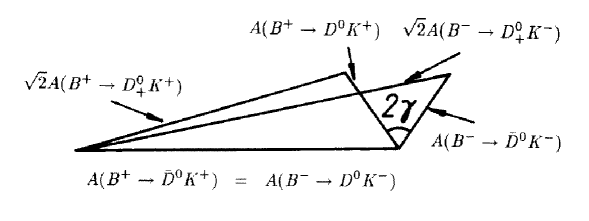
Figure 6: Triangle relations among $B^{\pm}\to DK^{\pm}$ decay amplitudes.

Combining all these considerations, we conclude that the triangle relations (148) and (149), which are depicted in Fig. 6, can be used to extract $\gamma$ by measuring only the rates of the corresponding six processes. This approach was proposed by Gronau and Wyler in Ref.^?. It is theoretically clean and suffers from no hadronic uncertainties. Unfortunately the triangles are expected to be very squashed ones since $B^{+}\to D^{0}K^{+}$ is both color- and CKM-suppressed with respect to $B^{+}\to\overline{D^{0}}K^{+}$:

$$\frac{|A(B^{+}\to D^{0}K^{+})|}{|A(B^{+}\to\overline{D^{0}}K^{+})|}=R_{b}\,\frac{|a|}{|A|}\approx 0.36\,\frac{a_{2}}{a_{1}}\approx 0.08.$$ (153)

Here $a_{1}$, $a_{2}$ are the usual phenomenological color-factors^?,? satisfying^? $a_{2}/a_{1}=0.26\pm 0.05\pm 0.09$. Using the $SU(3)$ flavor symmetry, the corresponding branching ratios can be estimated from the measured value^? $(5.3\pm 0.5)\cdot 10^{-3}$ of BR$(B^{+}\to\overline{D^{0}}\pi^{+})$ to be BR$(B^{+}\to\overline{D^{0}}K^{+})\approx 4\cdot 10^{-4}$ and BR$(B^{+}\to D^{0}K^{+})\approx 2\cdot 10^{-6}$. Another problem is related to the CP eigenstate of the neutral $D$ system. It is detected through $D^{0}_{+}\to\pi^{+}\pi^{-},K^{+}K^{-},\ldots$ and is experimentally challenging since the corresponding BR$\times$(detection efficiency) is expected to be at most of ${\cal O}(1\%)$. Therefore the Gronau-Wyler method^? will unfortunately be very difficult from an experimental point of view. A feasibility study can be found e.g. in Ref.^?.

A variant of the clean determination of $\gamma$ discussed above was proposed by Dunietz^? and uses the decays $B^{0}_{d}\to D^{0}_{+}K^{\ast 0}$, $B^{0}_{d}\to\overline{D^{0}}K^{\ast 0}$, $B^{0}_{d}\to D^{0}K^{\ast 0}$ and their charge-conjugates. Since these modes are “self-tagging” through $K^{\ast 0}\to K^{+}\pi^{-}$, no time-dependent measurements are needed in this method although neutral $B_{d}$ decays are involved. Compared to the Gronau-Wyler approach^?, both $B^{0}_{d}\to\overline{D^{0}}K^{\ast 0}$ and $B^{0}_{d}\to D^{0}K^{\ast 0}$ are color-suppressed, i.e.

$$\frac{|A(B^{0}_{d}\to D^{0}K^{\ast 0})|}{|A(B^{0}_{d}\to\overline{D^{0}}K^{\ast 0})|}\approx R_{b}\,\frac{a_{2}}{a_{2}}\approx 0.36.$$ (154)

Consequently the amplitude triangles are probably not as as squashed as in the $B^{\pm}\to DK^{\pm}$ case. The corresponding branching ratios are expected to be of ${\cal O}(10^{-5})$. Unfortunately one has also to deal with the difficulties of detecting the neutral $D$-meson CP eigenstate $D^{0}_{+}$.

3.6.2 $SU(3)$ Amplitude Relations

In a series of interesting papers^?,?, Gronau, Hernández, London and Rosner (GHLR) pointed out that the $SU(3)$ flavor symmetry of strong interactions^? – which appeared already several times in this review – can be combined with certain plausible dynamical assumptions, e.g. neglect of annihilation topologies, to derive amplitude relations among $B$ decays into $\pi\pi$, $\pi K$ and $K\overline{K}$ final states. These relations may allow determinations both of weak phases of the CKM matrix and of strong final state interaction phases by measuring only the corresponding branching ratios.

In order to illustrate this approach, let me describe briefly the “state of the art” one had about 3 years ago. At that time it was assumed that EW penguins should play a very minor role in non-leptonic $B$ decays and consequently their contributions were not taken into account. Within that approximation, which will be analyzed very carefully in Sections 4 and 5, the decay amplitudes for $B\to\{\pi\pi,\pi K,K\overline{K}\}$ transitions can be represented in the limit of an exact $SU(3)$ flavor symmetry in terms of five reduced matrix elements. This decomposition can also be performed in terms of diagrams. At the quark-level one finds six different topologies of Feynman diagrams contributing to $B\to\{\pi\pi,\pi K,K\overline{K}\}$ that show up in the corresponding decay amplitudes only as five independent linear combinations^?,?. In contrast to the classification of non-leptonic $B$ decays performed in Subsection 2.1, these six topologies of Feynman diagrams include also three non-spectator diagrams, i.e. annihilation processes, where the decaying $b$-quark interacts with its partner anti-quark in the $B$-meson. However, due to dynamical reasons, these three contributions are expected to be suppressed relative to the others and hence should play a very minor role. Consequently, neglecting these diagrams, $6-3=3$ topologies of Feynman diagrams suffice to represent the transition amplitudes of $B$ decays into $\pi\pi$, $\pi K$ and $K\overline{K}$ final states. To be specific, these diagrams describe “color-allowed” and “color-suppressed” current-current processes $T$ $(T^{\prime})$ and $C$ $(C^{\prime})$, respectively, and QCD penguins $P$ $(P^{\prime})$. As in Refs.^?,? and in 3.4.2, an unprimed amplitude denotes strangeness-preserving decays, whereas a primed amplitude stands for strangeness-changing transitions. Note that the color-suppressed topologies $C$ and $C^{\prime}$ involve the color-suppression factor^?-? $a_{2}\approx 0.2$.

Let us consider the decays $B^{+}\to\{\pi^{+}\pi^{0},\pi^{+}K^{0},\pi^{0}K^{+}\}$, i.e. the “original” GRL method^?, as an example. Neglecting both EW penguins, which will be discussed later, and the dynamically suppressed non-spectator contributions mentioned above, the decay amplitudes of these modes can be expressed as

$$\begin{array}[]{rcl}\sqrt{2}\,A(B^{+}\to\pi^{+}\pi^{0})&=&-\left(T+C\right)\\ A(B^{+}\to\pi^{+}K^{0})&=&P^{\prime}\\ \sqrt{2}\,A(B^{+}\to\pi^{0}K^{+})&=&-\left(T^{\prime}+C^{\prime}+P^{\prime}\right)\end{array}$$ (155)

with

$$T=|T|\,e^{i\gamma}\,e^{i\delta_{T}},\quad C=|C|\,e^{i\gamma}\,e^{i\delta_{C}}.$$ (156)

Here $\delta_{T}$ and $\delta_{C}$ denote CP-conserving strong phases. Using the $SU(3)$ flavor symmetry, the strangeness-changing amplitudes $T^{\prime}$ and $C^{\prime}$ can be obtained easily from the strangeness-preserving ones through

$$\frac{T^{\prime}}{T}\approx\frac{C^{\prime}}{C}\approx\lambda\frac{f_{K}}{f_{\pi}}\equiv r_{u},$$ (157)

where $f_{K}$ and $f_{\pi}$ take into account factorizable $SU(3)$-breaking corrections as in (122). The structures of the $\bar{b}\to\bar{d}$ and $\bar{b}\to\bar{s}$ QCD penguin amplitudes $P$ and $P^{\prime}$ corresponding to $P^{(d)}$ and $P^{(s)}$ (see (95) and (96)), respectively, have been discussed in 3.3.4. It is an easy exercise to combine the decay amplitudes given in (155) appropriately to derive the relations

$$\sqrt{2}\,A(B^{+}\to\pi^{0}K^{+})+A(B^{+}\to\pi^{+}K^{0}) = r_{u}\sqrt{2}\,A(B^{+}\to\pi^{+}\pi^{0})$$ (158)

$$\sqrt{2}\,A(B^{-}\to\pi^{0}K^{-})+A(B^{-}\to\pi^{-}\overline{K^{0}}) = r_{u}\sqrt{2}\,A(B^{-}\to\pi^{-}\pi^{0}),$$ (159)

which can be represented as two triangles in the complex plane. If one measures the rates of the corresponding six decays, these triangles can easily be constructed. Their relative orientation is fixed through $A(B^{+}\to\pi^{+}K^{0})=A(B^{-}\to\pi^{-}\overline{K^{0}})$, which is due to the fact that there is no non-trivial CP-violating weak phase present in the $\bar{b}\to\bar{s}$ QCD penguin amplitude governing $B^{+}\to\pi^{+}K^{0}$ as we have seen in 3.3.4. Taking into account moreover (156), we conclude that these triangles should allow a determination of $\gamma$ as can be seen in Fig. 7. From the geometrical point of view, that GRL approach^? is very similar to the $B^{\pm}\to DK^{\pm}$ construction^? shown in Fig. 6. Furthermore it involves also only charged $B$ decays and therefore neither time-dependent measurements nor tagging are required. In comparison with the Gronau-Wyler method^?, at first sight the major advantage of the GRL strategy seems to be that all branching ratios are expected to be of the same order of magnitude ${\cal O}(10^{-5})$, i.e. the corresponding triangles are not squashed ones, and that the difficult to measure CP eigenstate $D^{0}_{+}$ is not required.

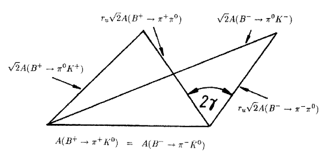
Figure 7: Naïve $SU(3)$ triangle relations among $B^{+}\to\{\pi^{+}\pi^{0},\pi^{+}K^{0},\pi^{0}K^{+}\}$ and charge-conjugate decay amplitudes neglecting EW penguin contributions.

However, things are unfortunately not that simple and – despite of its attractiveness – the general GHLR approach^?,? to extract CKM phases from $SU(3)$ amplitude relations suffers from theoretical limitations. The most obvious limitation is of course related to the fact that the relations are not, as e.g. (148) or (149), valid exactly but suffer from $SU(3)$-breaking corrections^?. While factorizable $SU(3)$-breaking can be included straightforwardly through certain meson decay constants or form factors, non-factorizable $SU(3)$-breaking corrections cannot be described in a reliable quantitative way at present. Another limitation is related to $\bar{b}\to\bar{d}$ QCD penguin topologies with internal up- and charm-quark exchanges which may affect the simple relation (101) between $\beta$ and the $\bar{b}\to\bar{d}$ QCD penguin amplitude $P$ significantly as we have seen in 3.3.4. Consequently these contributions may preclude reliable extractions of $\beta$ using $SU(3)$ amplitude relations and the assumption that $\bar{b}\to\bar{d}$ QCD penguin amplitudes are dominated by internal top-quark exchanges^? (see also 3.3.6). Remarkably also EW penguins^?,?,?, which we have neglected in our discussion of $SU(3)$ amplitude relations so far, have a very important impact on some $SU(3)$ constructions, in particular on the GRL method^? of determining $\gamma$. As we will see in Section 5, this approach is even spoiled by these contributions^?,?. However, there are other – generally more involved – $SU(3)$ methods^?-? that are not affected by EW penguins. Interestingly it is in principle also possible to shed light on the physics of these operators by using $SU(3)$ amplitude relations^?,?. This issue has been one of the “hot topics” in $B$ physics over the last few years and will be the subject of the remainder of this review. Before we shall investigate the role of EW penguins in methods for extracting angles of the UT in Section 5, let us in the following section have a closer look at a few non-leptonic $B$ decays that are affected significantly by EW penguin operators.

Figure 8: The dependence of the Wilson coefficients (28) on the top-quark mass $m_{t}$ for $\mu=m_{b}$ and $\Lambda_{\overline{\mbox{{\scriptsize MS}}}}=0.3\,\mbox{GeV}$ corresponding to four active quark flavors.

4 Electroweak Penguin Effects in Non-leptonic $B$-Meson Decays

Since the ratio $\alpha/\alpha_{s}={\cal O}(10^{-2})$ of the QED and QCD couplings is very small, one would expect that EW penguins should only play a minor role in comparison with QCD penguins. That would indeed be the case if the top-quark was not “heavy”. However, the Wilson coefficient of one EW penguin operator – the operator $Q_{9}$ specified in (18) – increases strongly with the top-quark mass as can be seen nicely in Fig. 8. There the $m_{t}$-dependence of the coefficients (28), which correspond to the case where the proper renormalization group evolution from $\mu={\cal O}(M_{W})$ down to $\mu={\cal O}(m_{b})$ has been neglected, is shown. A very similar behavior is also exhibited by the NLO Wilson coefficients^?. Consequently interesting EW penguin effects may arise from this feature in certain non-leptonic $B$ decays because of the large top-quark mass that has been measured^?,? recently with impressive accuracy^? by the CDF and D0 collaborations to be $m_{t}^{\mbox{{\scriptsize Pole}}}=(175\pm 6)\,\mbox{GeV}$. The parameter $m_{t}$ used in analyses of non-leptonic weak decays is, however, not equal to that measured “pole” mass^?. In NLO calculations, $m_{t}$ refers to the running top-quark current-mass normalized at the scale $\mu=m_{t}$, i.e. $\overline{m}_{t}(m_{t})$, which is typically by $8\,\mbox{GeV}$ smaller than $m_{t}^{\mbox{{\scriptsize Pole}}}$ for $m_{t}={\cal O}(170\,\mbox{GeV})$. The EW penguin effects discussed in the following subsections were pointed out first in Refs.^?,?,?. Meanwhile they were confirmed by several other authors^?,?,?-?.

Figure 9: The dependence of the ratio $R\propto\mbox{BR}(B^{+}\to K^{+}\phi)/\mbox{BR}(B^{+}\to\pi^{+}K^{\ast 0})$ on $m_{t}$ using the Wilson coefficients (28).

4.1 EW Penguin Effects in $B^{+}\to K^{+}\phi$ and $B^{+}\to\pi^{+}K^{\ast 0}$

The channels $B^{+}\to K^{+}\phi$ and $B^{+}\to\pi^{+}K^{\ast 0}$ originating from the penguin-induced $\bar{b}$-quark decays $\bar{b}\to\bar{s}s\bar{s}$ and $\bar{b}\to\bar{s}d\bar{d}$, respectively, are very similar from a QCD point of view, i.e. as far as their QCD penguin contributions are concerned. This feature is obvious if one draws the corresponding Feynman diagrams which is an easy exercise. However, an important difference arises in respect of EW penguin contributions. We have to deal both with small color-suppressed and sizable color-allowed EW penguin diagrams. Whereas the former contributions are again very similar for $B^{+}\to K^{+}\phi$ and $B^{+}\to\pi^{+}K^{\ast 0}$, the color-allowed EW penguin contributions are absent in the $B^{+}\to\pi^{+}K^{\ast 0}$ case and contribute only to $B^{+}\to K^{+}\phi$. Consequently significant EW penguin effects^? are expected in the mode $B^{+}\to K^{+}\phi$, while these effects should be negligible in the decay $B^{+}\to\pi^{+}K^{\ast 0}$.

This rather qualitative kind of reasoning is in agreement with the results of certain model calculations^?,?, where the formalism scetched in Section 2 was applied in combination with the “factorization” hypothesis^?,?. By factorization one means that the hadronic matrix elements of the four-quark operators appearing in the low energy effective Hamiltonian (15) are factorized into the product of hadronic matrix elements of two quark-currents that are described by a set of form factors. Usually the model proposed by Bauer, Stech and Wirbel^? (BSW) is used for these form factors and was also applied in Refs.^?,?. In contrast to color-allowed current-current processes, where “factorization” may work reasonably well^?, this assumption is questionable for penguin processes which are classical examples of non-factorizable diagrams. Nevertheless this approach may give us a feeling for the expected orders of magnitudes. Unfortunately a more reliable analytical way of dealing with non-leptonic $B$ decays is not available at present.

The corresponding calculations are quite complicated and a discussion of their technicalities would not be useful in the context of this review. Let me therefore just briefly discuss the main results. The model calculations indicate that EW penguins lead to a reduction of BR$(B^{+}\to K^{+}\phi)$ by ${\cal O}(30\%)$ for $m_{t}={\cal O}(170\,\mbox{GeV})$, while these effects are below $2\%$ in the case of BR$(B^{+}\to\pi^{+}K^{\ast 0})$. As in Fig. 5, the branching ratios, which are both of ${\cal O}(10^{-5})$, depend strongly on $k^{2}$, the four-momentum of the gluons and photons appearing in the penguin diagram depicted in Fig. 3. This “unphysical” $k^{2}$-dependence^? is due to the use of the above mentioned model. In order to reduce this dependence as well as other hadronic uncertainties, the ratio^?

$$R\equiv\left[\frac{f_{K^{\ast}}F_{B\pi}(M_{K^{\ast}}^{2};1^{-})}{f_{\phi}F_{BK}(M_{\phi}^{2};1^{-})}\right]^{2}\left[\frac{\Phi(M_{\pi}/M_{B},M_{K^{\ast}}/M_{B})}{\Phi(M_{K}/M_{B},M_{\phi}/M_{B})}\right]^{3}$$ (160)

$$\times\left[\frac{\mbox{BR}(B^{+}\to K^{+}\phi)}{\mbox{BR}(B^{+}\to\pi^{+}K^{\ast 0})}\right]\approx 0.5\times\left[\frac{\mbox{BR}(B^{+}\to K^{+}\phi)}{\mbox{BR}(B^{+}\to\pi^{+}K^{\ast 0})}\right],$$

where $f_{V}$ are meson decay constants, $F_{PP^{\prime}}$ are quark-current form factors and $\Phi(x,y)$ is the usual two-body phase space function, turns out to be very useful. Although $R$ is affected in almost the same way by EW penguins as the branching ratio BR$(B^{+}\to K^{+}\phi)$, it suffers much less from hadronic uncertainties, is very stable against variations both of the momentum transfer $k^{2}/m_{b}^{2}$ and of the QCD scale parameter $\Lambda_{\overline{\mbox{{\scriptsize MS}}}}$, and does not depend on CKM factors if the ${\cal O}(\lambda^{2})$ terms in (94) are neglected. These terms play a minor role and may lead to tiny direct CP-violating asymmetries of ${\cal O}(1\%)$. One should keep in mind, however, that BR$(B^{+}\to K^{+}\phi)$ and BR$(B^{+}\to\pi^{+}K^{\ast 0})$ could receive quite different contributions in principle if “factorization” does not hold. Therefore $R$ could be affected by such unknown corrections.

The effect of the NLO renormalization group evolution from $\mu={\cal O}(M_{W})$ down to $\mu={\cal O}(m_{b})$, i.e. the difference between using exact NLO Wilson coefficients^? or (28), is rather small and gives an enhancement of the branching ratios by about ${\cal O}(10\%)$ and an even smaller enhancement in the case of $R$. Hence the use of the approximate Wilson coefficients (28) is justified. The effects of the EW penguins can be seen nicely in Fig. 9, where the top-quark mass dependence of $R$ calculated with the help of these coefficients is shown. Whereas the dashed line corresponds to the case where only QCD penguins are included, the solid line describes the calculation taking into account both QCD and EW penguin operators.

There are not only some non-leptonic $B$ decays that are affected significantly by EW penguins. There are even a few channels where the corresponding operators may play the dominant role as we will see in the following two subsections.

4.2 EW Penguin Effects in $B^{+}\to\pi^{+}\phi$

In respect of EW penguin effects, the mode $B^{+}\to\pi^{+}\phi$ is also quite interesting^?. Within the spectator model, it originates from the penguin-induced $\bar{b}$-quark decay $\bar{b}\to\bar{d}s\bar{s}$, where the $s\bar{s}$ pair hadronizes into the $\phi$-meson which is present in a color-singlet state. The $s$- and $\bar{s}$-quarks emerging from the gluons of the usual QCD penguin diagrams form, however, a color-octet state and consequently cannot build up that $\phi$-meson (see also 3.3.2). Thus, using both an appropriate NLO low energy effective Hamiltonian and the BSW model in combination with the factorization assumption to estimate the relevant hadronic matrix elements of the QCD penguin operators, one finds a very small branching ratio BR$\left.(B^{+}\to\pi^{+}\phi)\right|_{\mbox{{\scriptsize QCD}}}={\cal O}(10^{-10})$. The non-vanishing result is due to the renormalization group evolution from $\mu={\cal O}(M_{W})$ down to $\mu={\cal O}(m_{b})$. Neglecting this evolution, i.e. applying the approximate Wilson coefficients (28), would give a vanishing branching ratio because of the color-arguments given above. Since these arguments do not apply to EW penguins, their contributions are expected to become important^?. In fact, taking into account also these operators gives a branching ratio BR$\left.(B^{+}\to\pi^{+}\phi)\right|_{\mbox{{\scriptsize QCD+EW}}}={\cal O}(10^{-8})$ for $m_{t}={\cal O}(170\,\mbox{GeV})$ that increases strongly with the top-quark mass. Unfortunately the enhancement by a factor of ${\cal O}(10^{2})$ through EW penguins is not strong enough to make the decay $B^{+}\to\pi^{+}\phi$ measurable in the foreseeable future.

The color-arguments for the QCD penguins may be affected by additional soft gluon exchanges which are not under quantitative control at present. These contributions would show up as non-factorizable contributions to the hadronic matrix elements of the penguin operators which were neglected in Ref.^?. Nevertheless there is no doubt that EW penguins play a very important – probably even dominant – role in the decay $B^{+}\to\pi^{+}\phi$ and related modes like $B^{+}\to\rho^{+}\phi$.

4.3 EW Penguin Effects in $B_{s}\to\pi^{0}\phi$

The theoretical situation arising in the decay $B_{s}^{0}\to\pi^{0}\phi$ caused by $\bar{b}\to\bar{s}\,(u\bar{u},d\bar{d})$ quark-level transitions is much more favorable than in the previous two subsections because of the $SU(2)$ isospin symmetry of strong interactions. Let me therefore be more detailed in the presentation of that transition which is expected to be dominated by EW penguins^?. In contrast to the decays discussed in 4.1 and 4.2, it receives not only penguin but also current-current operator contributions at the tree level. The final state is an eigenstate of the CP operator with eigenvalue +1 and has strong isospin quantum numbers $(I,I_{3})=(1,0)$, whereas the initial state is an isospin singlet. Thus we have to deal with a $\Delta I=1$ transition.

Looking at the operator basis given in (16)-(18), we observe that the current-current operators $Q^{us}_{1/2}$ and the EW penguin operators can lead to final states both with isospin $I=0$ and $I=1$, whereas the QCD penguin operators give only final states with $I=0$. Therefore the $\Delta I=1$ transition $B_{s}\to\pi^{0}\phi$ receives no QCD penguin contributions and arises purely from the current-current operators $Q^{us}_{1/2}$ and the EW penguin operators. For the same reason, QCD penguin matrix elements of the current-current operators $Q_{2}^{us}$ and $Q_{2}^{cs}$ (see (24)) with up- and charm-quarks running as virtual particles in the loops, respectively, do not contribute to that decay. Consequently, using in addition the unitarity of the CKM matrix and applying the modified Wolfenstein parametrization (10) yielding

$$V_{us}^{\ast}V_{ub}=\lambda|V_{ub}|\,e^{-i\gamma},\quad V_{ts}^{\ast}V_{tb}=-|V_{ts}|=-|V_{cb}|(1+{\cal O}(\lambda^{2})),$$ (161)

the hadronic matrix element of the Hamiltonian (15) can be expressed as

$$\Bigl{\langle}\pi^{0}\phi\Bigl{|}{\cal H}_{\mbox{{\scriptsize eff}}}(\Delta B=-1)\Bigr{|}\overline{B^{0}_{s}}\Bigr{\rangle}=\frac{G_{\mbox{{\scriptsize F}}}}{\sqrt{2}}\,|V_{ts}|$$

$$\times\left[\lambda^{2}R_{b}\,e^{-i\gamma}\sum\limits_{k=1}^{2}\Bigl{\langle}\pi^{0}\phi\Bigl{|}Q_{k}^{us}(\mu)\Bigr{|}\overline{B^{0}_{s}}\Bigr{\rangle}C_{k}(\mu)+\sum\limits_{k=7}^{10}\Bigl{\langle}\pi^{0}\phi\Bigl{|}Q_{k}^{s}(\mu)\Bigr{|}\overline{B^{0}_{s}}\Bigr{\rangle}C_{k}(\mu)\right],$$

where the correction of ${\cal O}(\lambda^{2})$ in (161) has been omitted.

Neglecting EW penguin operators for a moment and applying the formalism developed in 3.2.2, we would find ${\cal A}_{\mbox{{\scriptsize CP}}}^{\mbox{{\scriptsize mix-ind}}}(B_{s}\to\pi^{0}\phi)=\sin(2\gamma)$. The approximation of neglecting EW penguin operator contributions to $B_{s}\to\pi^{0}\phi$ is, however, very bad since the current-current amplitude $A_{\mbox{{\scriptsize CC}}}$ is suppressed relative to the EW penguin part $A_{\mbox{{\scriptsize EW}}}$ by the CKM factor $\lambda^{2}R_{b}\approx 0.02$. Moreover the current-current operator contribution is color-suppressed by $a_{2}\approx 0.2$. On the other hand, in the presence of a heavy top-quark, the Wilson coefficient of the dominant EW penguin operator $Q_{9}^{s}$ contributing to $B_{s}\to\pi^{0}\phi$ in color-allowed form is of ${\cal O}(10^{-2})$ (see Fig. 8). Therefore we expect $|A_{\mbox{{\scriptsize EW}}}|/|A_{\mbox{{\scriptsize CC}}}|={\cal O}(10^{-2}/(0.02\cdot 0.2))={\cal O}(2.5)$ and conclude that EW penguins have not only to be taken into account in an analysis of $B_{s}\to\pi^{0}\phi$ but should even give the dominant contribution to that channel.

In order to simplify the following discussion, let us neglect the influence of QCD corrections to EW penguins for a moment. Then the Wilson coefficients of the corresponding operators are given by $\overline{C}^{(0)}_{k}(\mu)$ $(k\in\{7,\ldots,10\})$ specified in (28). Since $\overline{C}^{(0)}_{8}(\mu)$ and $\overline{C}^{(0)}_{10}(\mu)$ vanish, we have to consider only hadronic matrix elements of the operators $Q_{1/2}^{us}$, $Q_{7}^{s}$ and of the dominant EW penguin operator $Q_{9}^{s}$. For the evaluation of the hadronic matrix elements, it is convenient to perform a Fierz transformation of the current-current operators and to consider

$$Q_{1}^{us} = (\bar{u}u)_{\mbox{{\scriptsize V--A}}}(\bar{s}b)_{\mbox{{\scriptsize V--A}}}\,=\,{\cal Q}^{I=0}_{\mbox{{\scriptsize V--A}}}+{\cal Q}^{I=1}_{\mbox{{\scriptsize V--A}}}$$

$$Q_{2}^{us} = (\bar{u}_{\alpha}u_{\beta})_{\mbox{{\scriptsize V--A}}}(\bar{s}_{\beta}b_{\alpha})_{\mbox{{\scriptsize V--A}}}\,=\,\tilde{\cal Q}^{I=0}_{\mbox{{\scriptsize V--A}}}+\tilde{\cal Q}^{I=1}_{\mbox{{\scriptsize V--A}}}$$

$$Q_{7}^{s}\,\, = \left[(\bar{u}u)_{\mbox{{\scriptsize V+A}}}-\frac{1}{2}(\bar{d}d)_{\mbox{{\scriptsize V+A}}}\right](\bar{s}b)_{\mbox{{\scriptsize V--A}}}\,=\,\frac{1}{2}{\cal Q}^{I=0}_{\mbox{{\scriptsize V+A}}}+\frac{3}{2}{\cal Q}^{I=1}_{\mbox{{\scriptsize V+A}}}$$ (163)

$$Q_{9}^{s}\,\, = \left[\,(\bar{u}u)_{\mbox{{\scriptsize V--A}}}\,-\,\frac{1}{2}(\bar{d}d)_{\mbox{{\scriptsize V--A}}}\right](\bar{s}b)_{\mbox{{\scriptsize V--A}}}\,=\,\frac{1}{2}{\cal Q}^{I=0}_{\mbox{{\scriptsize V--A}}}+\frac{3}{2}{\cal Q}^{I=1}_{\mbox{{\scriptsize V--A}}}.$$

Here the parts of $Q_{7}^{s}$ and $Q_{9}^{s}$ with quark flavors $(\bar{s}s)(\bar{s}b)$ and $(\bar{c}c)(\bar{s}b)$, which do not contribute to $\overline{B_{s}^{0}}\to\pi^{0}\phi$, have been neglected and the following isospin operators have been introduced:

$${\cal Q}^{I=0}_{\mbox{{\scriptsize V$\pm$A}}} = \frac{1}{2}\left[(\bar{u}u)_{\mbox{{\scriptsize V$\pm$A}}}+(\bar{d}d)_{\mbox{{\scriptsize V$\pm$A}}}\right](\bar{s}b)_{\mbox{{\scriptsize V--A}}}$$

$${\cal Q}^{I=1}_{\mbox{{\scriptsize V$\pm$A}}} = \frac{1}{2}\left[(\bar{u}u)_{\mbox{{\scriptsize V$\pm$A}}}-(\bar{d}d)_{\mbox{{\scriptsize V$\pm$A}}}\right](\bar{s}b)_{\mbox{{\scriptsize V--A}}}$$

$$\tilde{\cal Q}^{I=0}_{\mbox{{\scriptsize V$\pm$A}}} = \frac{1}{2}\left[(\bar{u}_{\alpha}u_{\beta})_{\mbox{{\scriptsize V$\pm$A}}}+(\bar{d}_{\alpha}d_{\beta})_{\mbox{{\scriptsize V$\pm$A}}}\right](\bar{s}_{\beta}b_{\alpha})_{\mbox{{\scriptsize V--A}}}$$ (164)

$$\tilde{\cal Q}^{I=1}_{\mbox{{\scriptsize V$\pm$A}}} = \frac{1}{2}\left[(\bar{u}_{\alpha}u_{\beta})_{\mbox{{\scriptsize V$\pm$A}}}-(\bar{d}_{\alpha}d_{\beta})_{\mbox{{\scriptsize V$\pm$A}}}\right](\bar{s}_{\beta}b_{\alpha})_{\mbox{{\scriptsize V--A}}}.$$

Taking into account that $B_{s}\to\pi^{0}\phi$ is a $\Delta I=1$ transition and employing non-perturbative “$B$-parameters” to parametrize the hadronic matrix elements yields

$$\Bigl{\langle}\pi^{0}\phi\Bigl{|}Q_{1}^{us}(\mu)\Bigr{|}\overline{B_{s}^{0}}\Bigr{\rangle} = \Bigr{\langle}\pi^{0}\phi\Bigl{|}{\cal Q}^{I=1}_{\mbox{{\scriptsize V--A}}}(\mu)\Bigr{|}\overline{B_{s}^{0}}\Bigr{\rangle}\,=\,B_{\mbox{{\scriptsize V--A}}}(\mu)\,h\,=\,\frac{2}{3}\Bigl{\langle}\pi^{0}\phi\Bigl{|}Q_{9}^{s}(\mu)\Bigr{|}\overline{B_{s}^{0}}\Bigr{\rangle}$$

$$\Bigl{\langle}\pi^{0}\phi\Bigl{|}Q_{2}^{us}(\mu)\Bigr{|}\overline{B_{s}^{0}}\Bigr{\rangle} = \Bigl{\langle}\pi^{0}\phi\Bigl{|}\tilde{\cal Q}^{I=1}_{\mbox{{\scriptsize V--A}}}(\mu)\Bigr{|}\overline{B_{s}^{0}}\Bigr{\rangle}\,=\,\frac{1}{3}\tilde{B}_{\mbox{{\scriptsize V--A}}}(\mu)\,h$$ (165)

$$\Bigl{\langle}\pi^{0}\phi\Bigl{|}Q_{7}^{s}(\mu)\Bigr{|}\overline{B_{s}^{0}}\Bigr{\rangle} = \frac{3}{2}\Bigl{\langle}\pi^{0}\phi\Bigl{|}{\cal Q}^{I=1}_{\mbox{{\scriptsize V+A}}}(\mu)\Bigr{|}\overline{B_{s}^{0}}\Bigr{\rangle}=\frac{3}{2}B_{\mbox{{\scriptsize V+A}}}(\mu)\,h,$$

where $h$ corresponds to the “factorized” matrix element $\bigl{\langle}\pi^{0}\phi\bigl{|}Q_{1}^{us}\bigr{|}\overline{B_{s}^{0}}\bigr{\rangle}$:

$$h=i\,\frac{f_{\pi}}{\sqrt{2}}\,i\,2\,M_{\phi}\,F_{B_{s}\phi}(M_{\pi}^{2};0^{-})\,(\varepsilon_{\phi}\cdot p_{B_{s}}).$$ (166)

Since the $\pi^{0}$-meson is a pseudoscalar particle and emerges from the axial vector parts of the quark-currents $\left[(\bar{u}u)_{\mbox{{\scriptsize V$\pm$A}}}-(\bar{d}d)_{\mbox{{\scriptsize V$\pm$A}}}\right]$, it is quite natural to assume

$$B_{\mbox{{\scriptsize V+A}}}(\mu)\approx-B_{\mbox{{\scriptsize V--A}}}(\mu).$$ (167)

For a similar reason, the one-loop QED penguin matrix elements of the current-current operators $Q_{1/2}^{us}$ and $Q_{1/2}^{cs}$, which have to be taken into account in order to have a consistent calculation (see Subsection 2.3), vanish, since the virtual photons appearing in the QED penguin diagrams generate $(\bar{u}u)_{\mbox{{\scriptsize V}}}$ and $(\bar{d}d)_{\mbox{{\scriptsize V}}}$ vector currents that cannot create the pseudoscalar $\pi^{0}$-meson. Consequently we obtain

$$\Bigl{\langle}\pi^{0}\phi\Bigl{|}{\cal H}_{\mbox{{\scriptsize eff}}}(\Delta B=-1)\Bigr{|}\overline{B^{0}_{s}}\Bigr{\rangle}=\frac{G_{\mbox{{\scriptsize F}}}}{\sqrt{2}}\,|V_{ts}|\,B_{\mbox{{\scriptsize V--A}}}(\mu)\,h$$

$$\times\left[\lambda^{2}R_{b}\,e^{-i\gamma}\left\{C_{1}(\mu)+\frac{1}{3}\frac{\tilde{B}_{\mbox{{\scriptsize V--A}}}(\mu)}{B_{\mbox{{\scriptsize V--A}}}(\mu)}C_{2}(\mu)\right\}+\frac{3}{2}\left\{\overline{C_{9}}^{(0)}(\mu)-\overline{C_{7}}^{(0)}(\mu)\right\}\right],$$

so that the CP-violating observables can be expressed as

$${\cal A}_{\mbox{{\scriptsize CP}}}^{\mbox{{\scriptsize dir}}}(B_{s}\to\pi^{0}\phi)=0,\quad{\cal A}_{\mbox{{\scriptsize CP}}}^{\mbox{{\scriptsize mix-ind}}}(B_{s}\to\pi^{0}\phi)=\frac{2\,(x+\cos\gamma)\sin\gamma}{x^{2}+2\,x\cos\gamma+1},$$ (169)

while the branching ratio BR$(B_{s}\to\pi^{0}\phi)$ takes the form

Figure 10: The dependence of ${\cal A}_{\mbox{{\scriptsize CP}}}^{\mbox{{\scriptsize mix-ind}}}(B_{s}\to\pi^{0}\phi)$ on $\gamma$ for various values of $x$.

$${\cal R}\equiv\frac{\mbox{BR}(B_{s}\to\pi^{0}\phi)}{\mbox{BR}_{\mbox{{\scriptsize CC}}}(B_{s}\to\pi^{0}\phi)}=x^{2}+2\,x\cos\gamma+1,$$ (170)

where $\mbox{BR}_{\mbox{{\scriptsize CC}}}(B_{s}\to\pi^{0}\phi)={\cal O}(10^{-8})$ denotes the current-current branching ratio. In these equations, $x$ describes the ratio of the contribution of the EW penguin operators to that of the current-current operators:

$$x\equiv\frac{A_{\mbox{{\scriptsize EW}}}}{A_{\mbox{{\scriptsize CC}}}}=\frac{3\left[\overline{C}_{9}^{(0)}(\mu)-\overline{C}_{7}^{(0)}(\mu)\right]}{2\lambda^{2}R_{b}\left[C_{1}(\mu)+\frac{1}{3}\frac{\tilde{B}_{\mbox{{\scriptsize V--A}}}(\mu)}{B_{\mbox{{\scriptsize V--A}}}(\mu)}C_{2}(\mu)\right]}\,.$$ (171)

Note that deviations from the relation (167) would only lead to very small corrections to (171) since $\overline{C}_{7}^{(0)}(\mu)$ is suppressed relative to $\overline{C}_{9}^{(0)}(\mu)$ by a factor of ${\cal O}(10^{-2})$. To eliminate the hadronic uncertainties in (171), we identify the combination of the Wilson coefficient functions $C_{1/2}(\mu)$ and the corresponding $B$-parameters with the phenomenological color-suppression factor^?-?

$$a_{2}\approx C_{1}(\mu)+\frac{1}{3}\frac{\tilde{B}_{\mbox{{\scriptsize V--A}}}(\mu)}{B_{\mbox{{\scriptsize V--A}}}(\mu)}C_{2}(\mu).$$ (172)

Applying the analytical expressions for the Wilson coefficients $\overline{C}_{7}^{(0)}(\mu)$ and $\overline{C}_{9}^{(0)}(\mu)$ given in (28), their $\mu$-dependences cancel explicitly so that we arrive at the $\mu$-independent expression

$$x\approx\frac{\alpha}{2\pi\lambda^{2}R_{b}\,a_{2}\sin^{2}\Theta_{\mbox{{\scriptsize W}}}}\bigl{[}5B(x_{t})-2C(x_{t})\bigr{]},$$ (173)

where the Inami-Lim functions^? $B(x_{t})$ and $C(x_{t})$ are given in (29) and describe box diagrams and $Z$ penguins, respectively. The photon penguin contributions to $\overline{C}^{(0)}_{7}(\mu)$ and $\overline{C}^{(0)}_{9}(\mu)$ described by the Inami-Lim function $D(x_{t})$ cancel in (173) because of the remark after (167).

Figure 11: The dependence of $\mbox{BR}(B_{s}\to\pi^{0}\phi)/\mbox{BR}_{\mbox{{\scriptsize CC}}}(B_{s}\to\pi^{0}\phi)$ on $\gamma$ for various values of $x$.

Note that (173) is rather clean concerning hadronic uncertainties. This nice feature is due to the fact that we are in a position to absorb all non-perturbative $B$-parameters related to deviations from naïve factorization of the hadronic matrix elements by introducing the phenomenological color-suppression factor $a_{2}$. Concerning short-distance QCD corrections, which have been neglected so far, we have to consider only those affecting the box diagrams and $Z$ penguins contributing to $x$, since the QCD corrections to the current-current operators are incorporated effectively in $a_{2}$. The corresponding short-distance QCD corrections are small if we use $\overline{m}_{t}(m_{t})$ as has to be done in NLO analyses of weak decays^?,?. Applying on the other hand the formalism described briefly in Section 2, one finds that the QCD corrections to EW penguin operators arising from the renormalization group evolution from $\mu={\cal O}(M_{W})$ down to $\mu={\cal O}(m_{b})$ modify $x$ by only a few percent and are hence also negligibly small.

Using as an example $a_{2}=0.25$, $R_{b}=0.36$ and $m_{t}=170\,\mbox{GeV}$ yields $x\approx-3$ and confirms nicely our qualitative expectation that EW penguins should play the dominant role in $B_{s}\to\pi^{0}\phi$. Varying $a_{2}$ within $0.2\,\,\mbox{{\scriptsize$\stackrel{{\scriptstyle<}}{{\sim}}$}}\,\,a_{2}\,\,\mbox{{\scriptsize$\stackrel{{\scriptstyle<}}{{\sim}}$}}\,\,0.3$ and $R_{b}$ and $m_{t}$ within their presently allowed experimental ranges gives $-5\,\,\mbox{{\scriptsize$\stackrel{{\scriptstyle<}}{{\sim}}$}}\,\,x\,\,\mbox{{\scriptsize$\stackrel{{\scriptstyle<}}{{\sim}}$}}-2$. The EW penguin contributions lead to dramatic effects in the mixing-induced CP asymmetry as well as in the branching ratio as can be seen nicely in Figs. 10 and 11, where the dependences of ${\cal A}_{\mbox{{\scriptsize CP}}}^{\mbox{{\scriptsize mix-ind}}}(B_{s}\to\pi^{0}\phi)$ and of the ratio ${\cal R}$ on $\gamma$ are shown for various values of $x$. The solid lines in these figures correspond to the case where EW penguins are neglected completely. In the case of ${\cal A}_{\mbox{{\scriptsize CP}}}^{\mbox{{\scriptsize mix-ind}}}(B_{s}\to\pi^{0}\phi)$ even the sign is changed through the EW penguin contributions for $\gamma<90^{\circ}$, whereas the branching ratio is enhanced by a factor of ${\cal O}(10)$ with respect to the pure current-current case. The resulting BR$(B_{s}\to\pi^{0}\phi)$ is of ${\cal O}(10^{-7})$, so that an experimental investigation of that decay – which would be interesting to explore EW penguins – will unfortunately be very difficult. Needless to say, the modes $B_{s}\to\rho^{0}\phi,\pi^{0}\eta,\rho^{0}\eta$ exhibiting a very similar dynamics should also be dominated by their EW penguin contributions^?,?.

5 The Role of EW Penguins in Strategies for Extracting CKM Phases

In the strategies for extracting CKM phases reviewed in Section 3, EW penguins do not lead to problems wherever it has not been emphasized explicitly. That is in fact the case for most of these methods. However, the GL approach^? to eliminate the penguin uncertainties affecting the determination of $\alpha$ from ${\cal A}_{\mbox{{\scriptsize CP}}}^{\mbox{{\scriptsize mix-ind}}}(B_{d}\to\pi^{+}\pi^{-})$ with the help of isospin relations among $B\to\pi\pi$ decays (see 3.3.3), as well as the GRL method^? to determine $\gamma$ from $SU(3)$ amplitude relations involving $B^{+}\to\{\pi^{+}\pi^{0},\pi^{+}K^{0},\pi^{0}K^{+}\}$ and their charge-conjugates (see 3.6.2) require a careful investigation^?,?,?.

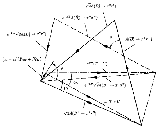
Figure 12: The determination of $\alpha$ from $B\to\pi\pi$ isospin triangles in the presence of EW penguins.

5.1 The GL Method of Extracting $\alpha$

If one redraws the GL construction^? to determine $\alpha$ from $B\to\pi\pi$ isospin triangles by taking into account EW penguin contributions, one obtains the situation shown in Fig. 12. This construction^? is a bit different from the original one presented in Ref.^?, since the $A(\overline{B}\to\pi\pi)$ amplitudes have been rotated by $e^{-2i\beta}$. The angle $\phi$ fixing the relative orientation of the two isospin triangles, which are constructed by measuring only the corresponding six branching ratios, is determined from the mixing-induced CP asymmetry of $B_{d}\to\pi^{+}\pi^{-}$ with the help of the relation

$${\cal A}_{\mbox{{\scriptsize CP}}}^{\mbox{{\scriptsize mix-ind}}}(B_{d}\to\pi^{+}\pi^{-})=-\,\frac{2\,\bigl{|}A(\overline{B^{0}_{d}}\to\pi^{+}\pi^{-})\bigr{|}\bigl{|}A(B^{0}_{d}\to\pi^{+}\pi^{-})\bigr{|}}{\bigl{|}A(\overline{B^{0}_{d}}\to\pi^{+}\pi^{-})\bigr{|}^{2}+\bigl{|}A(B^{0}_{d}\to\pi^{+}\pi^{-})\bigr{|}^{2}}\,\sin\phi\,.$$ (174)

In Fig. 12, the notation of GHLR^? has been used, where $P_{\mbox{{\scriptsize EW}}}$ and $P_{\mbox{{\scriptsize EW}}}^{\mbox{{\scriptsize C}}}$ denote color-allowed and color-suppressed $\bar{b}\to\bar{d}$ EW penguin amplitudes and $c_{u}=+2/3$ and $c_{d}=-1/3$ are the electrical up- and down-type quark charges, respectively. Because of the presence of EW penguins, the construction shown in that figure does not allow the determination of the exact angle $\alpha$ of the UT. It allows only the extraction of an angle $\tilde{\alpha}$ that is related to $\alpha$ through

$$\alpha=\tilde{\alpha}+\Delta\alpha,$$ (175)

where $\Delta\alpha$ is given by

$$\Delta\alpha=r\,\sin\alpha\,\cos\,(\rho-\alpha)+{\cal O}(r^{2})$$ (176)

with

$$r\equiv\frac{\left|(c_{u}-c_{d})(P_{\mbox{{\scriptsize EW}}}+P_{\mbox{{\scriptsize EW}}}^{\mbox{{\scriptsize C}}})\right|}{|T+C|}\approx\left|\frac{P_{\mbox{{\scriptsize EW}}}}{T}\right|.$$ (177)

Since $r$ is expected to be of ${\cal O}(0.2^{2})$ as can be shown by using a plausible hierarchy of $\bar{b}\to\bar{d}$ decay amplitudes ^?, EW penguins should not lead to serious problems in the GL method. This statement can also be put on more quantitative ground. Unfortunately $\rho$ contains strong final state interaction phases and hence cannot be calculated at present. However, using $|\cos(\rho-\alpha)|\leq 1$, one may estimate the following upper bound^? for the uncertainty $\Delta\alpha$:

$$|\Delta\alpha|\,\,\mbox{{\scriptsize$\stackrel{{\scriptstyle<}}{{\sim}}$}}\,\,\frac{\alpha}{2\pi a_{1}\sin^{2}\Theta_{\mbox{{\scriptsize W}}}}\bigl{|}5B(x_{t})-2C(x_{t})\bigr{|}\cdot\left|\frac{V_{td}}{V_{ub}}\right|\left|\sin\alpha\right|\,.$$ (178)

Taking into account the present status of the CKM matrix yielding the upper limit^? $|V_{td}|/|V_{ub}|\leq 4.6$ gives $|\Delta\alpha|/|\sin\alpha|\,\,\mbox{{\scriptsize$\stackrel{{\scriptstyle<}}{{\sim}}$}}\,4^{\circ}$ for a top-quark mass $m_{t}=170\,\mbox{GeV}$ and a phenomenological color-factor $a_{1}=1$.

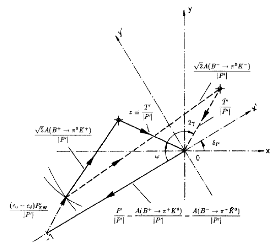
Figure 13: $SU(3)$ relations among $B^{+}\to\{\pi^{+}\pi^{0},\pi^{+}K^{0},\pi^{0}K^{+}\}$ and charge-conjugate decay amplitudes including EW penguin contributions.

5.2 The GRL Method of Extracting $\gamma$

In the case of the GRL strategy^? for extracting the UT angle $\gamma$ from the construction shown in Fig. 7, we have to deal with $\bar{b}\to\bar{s}$ modes which exhibit an interesting hierarchy of decay amplitudes^?,? that is very different from the $\bar{b}\to\bar{d}$ case discussed in the previous subsection. Since the color-allowed current-current amplitude $T^{\prime}$ is highly CKM suppressed by $\lambda^{2}R_{b}\approx 0.02$, one expects that the QCD penguin amplitude $P^{\prime}$ plays the dominant role in this decay class and that $T^{\prime}$ and the color-allowed EW penguin amplitude $P^{\prime}_{\mbox{{\scriptsize EW}}}$ are equally important^?:

$$\left|\frac{T^{\prime}}{P^{\prime}}\right|={\cal O}(0.2),\quad\left|\frac{P^{\prime}_{\mbox{{\scriptsize EW}}}}{T^{\prime}}\right|={\cal O}(1)\,.$$ (179)

The last ratio can be estimated more quantitatively^? as

$$\left|\frac{P^{\prime}_{\mbox{{\scriptsize EW}}}}{T^{\prime}}\right|\approx\frac{\alpha}{2\pi\lambda^{2}R_{b}\,a_{1}\sin^{2}\Theta_{\mbox{{\scriptsize W}}}}\bigl{|}5B(x_{t})-2C(x_{t})\bigr{|}\,r_{SU(3)}.$$ (180)

Here $r_{SU(3)}$ takes into account $SU(3)$-breaking corrections. Factorizable corrections are described by

$$\left.r_{SU(3)}\right|_{\mbox{{\scriptsize fact}}}=\frac{f_{\pi}}{f_{K}}\frac{F_{BK}(0;0^{+})}{F_{B\pi}(0;0^{+})},$$ (181)

where the BSW form factors^? parametrizing the corresponding quark-current matrix elements yield $\left.r_{SU(3)}\right|_{\mbox{{\scriptsize fact}}}\approx 1$. The ratio (180) increases significantly with the top-quark mass. Using $m_{t}=170\,\mbox{GeV}$, $R_{b}=0.36$, $a_{1}=1$ and $r_{SU(3)}=1$ gives $|P^{\prime}_{\mbox{{\scriptsize EW}}}|/|T^{\prime}|\approx 0.8$ and confirms nicely the expectation (179).

Consequently EW penguins are very important in that case and even spoil the GRL approach^? to determine $\gamma$ as was pointed out by Deshpande and He^?. This feature can be seen nicely in Fig. 13, where color-suppressed EW penguin and current-current amplitudes are neglected to simplify the presentation^?. If the EW penguin amplitude $(c_{u}-c_{d})\,P^{\prime}_{\mbox{{\scriptsize EW}}}$ were not there, this figure would correspond to Fig. 7 and we would simply have to deal with two triangles in the complex plane that could be fixed by measuring only the six branching ratios corresponding to $B^{+}\to\{\pi^{+}\pi^{0},\pi^{+}K^{0},\pi^{0}K^{+}\}$ and their charge-conjugates. However, EW penguins do contribute and since the magnitude of their “unknown” amplitude $(c_{u}-c_{d})\,P^{\prime}_{\mbox{{\scriptsize EW}}}$ is of the same size as $|T^{\prime}|$, it is unfortunately not possible to determine $\gamma$ with the help of this construction. This feature led to the development of other methods using $SU(3)$ amplitude relations to extract $\gamma$ that require also only measurements of branching ratios, and to strategies to control EW penguins in a quantitative way to shed light on the physics of these FCNC processes.

5.3 $SU(3)$ Strategies for Extracting $\gamma$ without EW Penguin Problems

In the recent literature^?-? some solutions have been proposed to solve the problem arising from EW penguins in the GRL approach. Let us have a closer look at them in this subsection.

Figure 14: Amplitude quadrangle for $B\to\pi K$ decays. The labels are explained in the text.

5.3.1 Amplitude Quadrangle for $B\to\pi K$ Decays

A quadrangle construction involving $B\to\pi K$ decay amplitudes was proposed in Ref.^? that can be used in principle to determine $\gamma$ irrespectively of the presence of EW penguins. This construction is shown in Fig. 14, where (a) corresponds to $A(B^{+}\to\pi^{+}K^{0})$, (b) to $\sqrt{2}\,A(B^{+}\to\pi^{0}K^{+})$, (c) to $\sqrt{2}\,A(B^{0}_{d}\to\pi^{0}K^{0})$, (d) to $A(B^{0}_{d}\to\pi^{-}K^{+})$ and the dashed line (e) to the decay amplitude $\sqrt{3}\,A(B_{s}^{0}\to\pi^{0}\eta)$. The dotted line (f) denotes an $I=3/2$ isospin amplitude $A_{3/2}$ that is composed of two parts and can be written as^?

$$A_{3/2}=\bigl{|}A_{\pi K}^{\mbox{{\scriptsize T}}}\bigr{|}\,e^{i\tilde{\delta}_{T}}\,e^{i\gamma}-\bigl{|}A_{\pi K}^{\mbox{{\scriptsize EWP}}}\bigr{|}\,e^{i\tilde{\delta}_{\mbox{{\scriptsize EWP}}}}\,.$$ (182)

The corresponding charge-conjugate amplitude takes on the other hand the form

$$\overline{A}_{3/2}=\bigl{|}A_{\pi K}^{\mbox{{\scriptsize T}}}\bigr{|}\,e^{i\tilde{\delta}_{T}}\,e^{-i\gamma}-\bigl{|}A_{\pi K}^{\mbox{{\scriptsize EWP}}}\bigr{|}\,e^{i\tilde{\delta}_{\mbox{{\scriptsize EWP}}}}\,,$$ (183)

so that the EW penguin contributions cancel in the difference of (182) and (183):

$$A_{3/2}-\overline{A}_{3/2}=2\,i\,e^{i\tilde{\delta}_{T}}\,\bigl{|}A_{\pi K}^{\mbox{{\scriptsize T}}}\bigr{|}\,\sin\gamma\,.$$ (184)

In order to determine this amplitude difference geometrically, both the quadrangle depicted in Fig. 14 and the one corresponding to the charge-conjugate processes have to be constructed by measuring the branching rations corresponding to (a)–(e). Moreover the relative orientation of these two quadrangles in the complex plane has to be fixed. This can be done easily through the side (a) as no non-trivial CP-violating weak phase is present in the $\bar{b}\to\bar{s}$ penguin-induced decay $B^{+}\to\pi^{+}K^{0}$, i.e.  $A(B^{-}\to\pi^{-}\overline{K^{0}})=A(B^{+}\to\pi^{+}K^{0})$ (see 3.3.4). Since the quantity $\bigl{|}A_{\pi K}^{\mbox{{\scriptsize T}}}\bigr{|}$ corresponds to $|T^{\prime}+C^{\prime}|$, it can be determined with the help of the $SU(3)$ flavor symmetry (note (155) and (157)) by measuring the branching ratio for $B^{+}\to\pi^{+}\pi^{-}$, i.e. through $\bigl{|}A_{\pi K}^{\mbox{{\scriptsize T}}}\bigr{|}=r_{u}\,\sqrt{2}\,|A(B^{+}\to\pi^{+}\pi^{0})|$, so that both $\sin\gamma$ and the strong phase $\tilde{\delta}_{T}$ can be extracted from the amplitude difference (184). Unfortunately the dashed line (e) corresponds to the decay $B^{0}_{s}\to\pi^{0}\eta$ that is dominated by EW penguins^?,? (see Subsection 4.3) and is therefore expected to exhibit a branching ratio at the ${\cal O}(10^{-7})$ level. Consequently the amplitude quadrangles are rather squashed ones and this approach to determine $\gamma$ is very difficult from an experimental point of view.

Figure 15: $SU(3)$ amplitude relations involving $B^{+}\to\{\pi^{+}K^{0},\pi^{0}K^{+},\eta_{8}\,K^{+}\}$ and charge-conjugates (dashed lines). The labels are explained in the text.

5.3.2 $SU(3)$ Relations among $B^{+}\to\{\pi^{+}K^{0},\pi^{0}K^{+},\eta_{8}\,K^{+}\}$ Decay Amplitudes

Another approach to extract $\gamma$ involving the decays $B^{+}\to\{\pi^{+}K^{0},\pi^{0}K^{+},\eta_{8}\,K^{+}\}$ and their charge-conjugates was proposed by Deshpande and He in Ref.^?. Using $SU(3)$ flavor symmetry, it is possible to derive relations among the corresponding decay amplitudes that can be represented in the complex plane as shown in Fig. 15. Here the solid lines labelled (a), (b) and (c) correspond to the decay amplitudes $A(B^{+}\to\pi^{+}K^{0})$, $\sqrt{2}\,A(B^{+}\to\pi^{0}K^{+})$ and $\sqrt{6}\,A(B^{+}\to\eta_{8}\,K^{+})$, respectively, and the dashed lines represent the corresponding charge-conjugate amplitudes. Note that $A(B^{-}\to\pi^{-}\overline{K^{0}})=A(B^{+}\to\pi^{+}K^{0})$ has also been used in this construction. Similarly as in 5.3.1, the determination of $\gamma$ can be accomplished by considering the difference of a particularly useful chosen combination $A$ of decay amplitudes and its charge-conjugate $\overline{A}$, where the penguin contributions cancel:

$$A-\overline{A}=2\,\sqrt{2}\,i\,e^{i\tilde{\delta}_{T}}r_{u}\,|A(B^{+}\to\pi^{+}\pi^{0})|\,\sin\gamma\,.$$ (185)

Here the magnitude of the $B^{+}\to\pi^{+}\pi^{0}$ amplitude is used – as in the $B\to\pi K$ quadrangle approach^? – to fix $|T^{\prime}+C^{\prime}|$. In Fig. 15, the dotted lines (x) and (y) represent two possible solutions for this amplitude difference. The fact that this construction does not give a unique solution for $A-\overline{A}$ is a well-known characteristic feature of all geometrical constructions of this kind, i.e. one has in general to deal with several discrete ambiguities.

Compared to the method using $B\to\pi K$ quadrangles discussed in 5.3.1, the advantage of this strategy is that all branching ratios are expected to be of the same order of magnitude ${\cal O}(10^{-5})$. In particular one has not to deal with an EW penguin dominated channel exhibiting a branching ratio at the ${\cal O}(10^{-7})$ level. However, the accuracy of the strategy is limited by $\eta-\eta^{\prime}$ mixing, i.e. the $A(B^{\pm}\to\eta_{8}\,K^{\pm})$ amplitudes have to be determined through

$$A(B^{\pm}\to\eta_{8}\,K^{\pm})=A(B^{\pm}\to\eta\,K^{\pm})\cos\Theta+A(B^{\pm}\to\eta^{\prime}K^{\pm})\sin\Theta$$ (186)

with a mixing angle $\Theta\approx 20^{\circ}$, and by other $SU(3)$-breaking effects which cannot be calculated at present. A similar approach to determine $\gamma$ was proposed by Gronau and Rosner in Ref.^?, where the amplitude construction is expressed in terms of the physical $\eta$ and $\eta^{\prime}$ states. A detailed discussion of $SU(3)$ amplitude relations for $B$ decays involving $\eta$ and $\eta^{\prime}$ in light of extractions of CKM phases can be found in Ref.^?.

5.3.3 A Simple Strategy for Fixing $\gamma$ and Obtaining Insights into the World of EW Penguins

Since the geometrical constructions discussed in 5.3.1 and 5.3.2 are quite complicated and appear to be very challenging from an experimental point of view, let us consider a much simpler approach^? to determine $\gamma$. It uses the decays $B^{+}\to\pi^{+}K^{0}$, $B^{0}_{d}\to\pi^{-}K^{+}$ and their charge-conjugates. In the case of these transitions, EW penguins contribute only in color-suppressed form and hence play a minor role. Neglecting these contributions and using the $SU(2)$ isospin symmetry of strong interactions – not $SU(3)$ – to relate their QCD penguin contributions (note the similarity to the example given in 3.4.2), the corresponding decay amplitudes can be written in the GHLR notation^? as

$$A(B^{+}\to\pi^{+}K^{0}) = P^{\prime}\,=\,A(B^{-}\to\pi^{-}\overline{K^{0}})$$

$$A(B^{0}_{d}\to\pi^{-}K^{+}) = -\,(P^{\prime}+T^{\prime})$$ (187)

$$A(\overline{B^{0}_{d}}\to\pi^{+}K^{-}) = -\,(P^{\prime}+e^{-2i\gamma}\,T^{\prime})\,.$$

Let me note that these relations are on rather solid ground from a theoretical point of view. They can be represented in the complex plane as shown in Fig. 16. Here (a) corresponds to $A(B^{+}\to\pi^{+}K^{0})=P^{\prime}=A(B^{-}\to\pi^{-}\overline{K^{0}})$, (b) to $A(B^{0}_{d}\to\pi^{-}K^{+})$, (c) to $A(\overline{B^{0}_{d}}\to\pi^{+}K^{-})$ and the dashed lines (d) and (e) to the color-allowed current-current amplitudes $T^{\prime}$ and $e^{-2i\gamma}\,T^{\prime}$, respectively. The dotted lines (f)–(h) will be discussed in a moment. Note that these $B\to\pi K$ decays appeared already in 3.3.6. Combining their branching ratios with the observables of a time-dependent measurement of $B_{d}\to\pi^{+}\pi^{-}$, a simultaneous extraction of $\alpha$ and $\gamma$ may be possible^?. The information provided by the $B\to\pi K$ modes can, however, also be used for a quite different approach that may finally allow the determination of EW penguin amplitudes.

Figure 16: $SU(2)$ isospin relations among $B^{+}\to\pi^{+}K^{0}$, $B^{0}_{d}\to\pi^{-}K^{+}$ and charge-conjugates. The labels are explained in the text.

In order to determine $\gamma$ from Fig 16, we have to know the length $|T^{\prime}|$ of the dashed lines (d) and (e). In fact, the situation is analogous to the extraction of $\gamma$ from (119) and (120) in 3.4.2. There we saw that $B^{+}\to\pi^{+}\pi^{0}$ provides an estimate of that quantity through (122) which is based on two assumptions: $SU(3)$ flavor symmetry and neglect of color-suppressed current-current contributions to $B^{+}\to\pi^{+}\pi^{0}$. Consequently, following these lines, it is possible to obtain an estimate of $\gamma$ by measuring only BR$(B^{+}\to\pi^{+}K^{0})=\mbox{BR}(B^{-}\to\pi^{-}\overline{K^{0}})$, BR$(B^{0}_{d}\to\pi^{-}K^{+})$, BR$(\overline{B^{0}_{d}}\to\pi^{+}K^{-})$ and BR$(B^{+}\to\pi^{+}\pi^{0})=\mbox{BR}(B^{-}\to\pi^{-}\pi^{0})$. Note that the neutral $B_{d}$ decays are “self-tagging” modes so that no time-dependent measurements are needed and that this estimate of $\gamma$ is very similar to the “original” GRL approach^? shown in Fig. 7 that is unfortunately spoiled by EW penguins. Needless to say, this strategy is very simple from a geometrical point of view – just triangle constructions – and very promising from an experimental point of view since all branching ratios are of the same order of magnitude ${\cal O}(10^{-5})$. Moreover no difficult to measure CP eigenstate of the neutral $D$ system is required as in 3.6.1.

Let me emphasize that the “weak” point of this approach – and of the one using untagged $B_{s}$ decays discussed in 3.4.2 – is the relation (122) to estimate $|T^{\prime}|$. Therefore the “estimate” of $\gamma$ may well turn into a solid “determination” if it should become possible to fix the magnitude of the color-allowed current-current amplitude contributing to $B^{0}_{d}\to\pi^{-}K^{+}$ in a more reliable way. Another possibility of fixing $|T^{\prime}|$ is of course the factorization hypothesis which may work reasonably well for that color-allowed amplitude^? and could be used as some kind of cross-check for (122). Maybe the “final” result for $|T^{\prime}|$ will come from lattice gauge theory one day.

Interestingly the construction shown in Fig. 16 provides even more information if one takes into account the amplitude relations

$$\sqrt{2}\,A(B^{+}\to\pi^{0}K^{+}) \approx -\,\left[P^{\prime}+T^{\prime}+(c_{u}-c_{d})P_{\mbox{{\scriptsize EW}}}^{\prime}\right]$$ (188)

$$\sqrt{2}\,A(B^{-}\to\pi^{0}K^{-}) \approx -\,\left[P^{\prime}+e^{-2i\gamma}\,T^{\prime}+(c_{u}-c_{d})P_{\mbox{{\scriptsize EW}}}^{\prime}\right],$$ (189)

where color-suppressed current-current and EW penguin amplitudes have been neglected. Consequently, the dotted lines (f) and (g) corresponding to $\sqrt{2}\,A(B^{+}\to\pi^{0}K^{+})$ and $\sqrt{2}\,A(B^{-}\to\pi^{0}K^{-})$, respectively, allow a determination of the dotted line (h) denoting the color-allowed $\bar{b}\to\bar{s}$ EW penguin amplitude $(c_{u}-c_{d})P_{\mbox{{\scriptsize EW}}}^{\prime}$. Since EW penguins are – in contrast to QCD penguins – dominated to excellent accuracy by internal top-quark exchanges, the $\bar{b}\to\bar{d}$ EW penguin amplitude $(c_{u}-c_{d})P_{\mbox{{\scriptsize EW}}}$ is related in the limit of an exact $SU(3)$ flavor symmetry to the corresponding $\bar{b}\to\bar{s}$ amplitude through the simple relation

$$(c_{u}-c_{d})P_{\mbox{{\scriptsize EW}}}=-\lambda\,R_{t}\,e^{-i\beta}\,(c_{u}-c_{d})P_{\mbox{{\scriptsize EW}}}^{\prime}$$ (190)

and may consequently be determined from the constructed $(c_{u}-c_{d})P_{\mbox{{\scriptsize EW}}}^{\prime}$ amplitude.

5.4 Towards Control over EW Penguins

It would be very useful to determine the EW penguin contributions experimentally. That would allow several predictions, consistency checks and tests of certain SM calculations^?. For example, one may determine the quantity $x$ introduced in (171) parametrizing the EW penguin effects in $B_{s}\to\pi^{0}\phi$ experimentally, and may compare this result with the SM expression (173). That way one may obtain predictions for ${\cal A}_{\mbox{{\scriptsize CP}}}^{\mbox{{\scriptsize mix-ind}}}(B_{s}\to\pi^{0}\phi)$ and BR$(B_{s}\to\pi^{0}\phi)$ long before it might be possible (if it is possible at all!) to measure them directly. Another interesting point is that the $\bar{b}\to\bar{d}$ EW penguin amplitude $P_{\mbox{{\scriptsize EW}}}$ allows in principle to fix the uncertainty $\Delta\alpha$ (see (175)) arising from EW penguins in the GL method^? of extracting $\alpha$ and to check whether it is e.g. in agreement with (178). Since EW penguins are “rare” FCNC processes that are absent at tree level within the SM, it may well be that “New Physics” contributes to them significantly through additionally present virtual particles in the loops. Consequently EW penguins may give hints to physics beyond the SM.

We have just seen an example of a simple strategy to determine EW penguin amplitudes experimentally. In Ref.^?, where more involved methods to accomplish this task are discussed, it was pointed out that the central input to control EW penguins in a quantitative way is the CKM angle $\gamma$. Consequently determinations of this UT angle are not only important in respect of testing the SM description of CP violation but also to shed light on the physics of EW penguins.

6 Summary and Concluding Remarks

The $B$-meson system provides a very fertile ground for studying CP violation and extracting CKM phases. In this respect neutral $B_{q}$ decays ($q\in\{d,s\}$) are particularly promising. The point is that “mixing-induced” CP-violating asymmetries are closely related to angles of the UT in some cases. For example, the “gold-plated” decay $B_{d}\to J/\psi\,K_{\mbox{{\scriptsize S}}}$ allows an extraction of $\sin(2\beta)$ to excellent accuracy because of its particular decay structure, and $B_{d}\to\pi^{+}\pi^{-}$ probes $\sin(2\alpha)$. However, hadronic uncertainties arising from QCD penguins preclude a theoretical clean determination of $\sin(2\alpha)$ by measuring only ${\cal A}_{\mbox{{\scriptsize CP}}}^{\mbox{{\scriptsize mix-ind}}}(B_{d}\to\pi^{+}\pi^{-})$. Consequently more involved strategies are required to extract $\alpha$. Such methods are fortunately already available and certainly time will tell which of them is most promising from an experimental point of view.

In the case of $B_{s}\to\rho^{0}K_{\mbox{{\scriptsize S}}}$, which appeared frequently in the literature as a tool to determine $\gamma$, penguin contributions are expected to lead to serious problems so that a meaningful extraction of $\gamma$ from this mode should not be possible. There are, however, other $B_{s}$ decays that may allow determinations of this UT angle, in some cases even in a clean way. Unfortunately $B^{0}_{s}-\overline{B^{0}_{s}}$ mixing may be too fast to be resolved with present vertex technology so that these strategies are experimentally very challenging.

An alternative route to extract CKM phases from $B_{s}$ decays and explore CP violation in these modes may be provided by the width difference of the $B_{s}$ system that is expected to be sizable. Interestingly the rapid oscillatory $\Delta M_{s}t$ terms cancel in untagged $B_{s}$ data samples that depend therefore only on two different exponents $e^{-\Gamma_{L}^{(s)}t}$ and $e^{-\Gamma_{H}^{(s)}t}$. Several strategies to extract $\gamma$ and the Wolfenstein parameter $\eta$ from untagged $B_{s}$ decays have been proposed recently. Here time-dependent angular distributions for $B_{s}$ decays into admixtures of CP eigenstates and exclusive channels that are caused by $\bar{b}\to\bar{u}c\bar{s}$ ($b\to c\bar{u}s$) quark-level transitions play a key role. Such untagged methods are obviously much more promising in respect of efficiency, acceptance and purity. However, their feasibility depends crucially on $\Delta\Gamma_{s}$ and it is not clear at present whether it will turn out to be large enough.

Theoretical analyses of CP violation in charged $B$ decays are usually very technical and suffer in general from large hadronic uncertainties. Consequently CP-violating asymmetries in charged $B$ decays are mainly interesting in view of excluding “superweak” models of CP violation in an unambiguous way. Nevertheless, if one combines branching ratios of charged $B$ decays in a clever way, they may allow determinations of angles of the UT, in some cases even without hadronic uncertainties.

To this end certain relations among decay amplitudes are used. The prototype of this approach are $B\to DK$ amplitude triangles that allow a clean determination of $\gamma$. Unfortunately one has to deal with experimental problems in that strategy of fixing this UT angle. Whereas the $B\to DK$ triangle relations are valid exactly, one may also use the $SU(3)$ flavor symmetry of strong interactions with certain plausible dynamical assumptions to derive approximate relations among non-leptonic $B\to\{\pi\pi,\pi K,K\overline{K}\}$ decay amplitudes which may allow extractions of CKM phases and strong final state interaction phases by measuring only the corresponding branching ratios. This approach has been very popular over the recent years. It suffers, however, from limitations due to non-factorizable $SU(3)$-breaking, QCD penguins with internal up- and charm-quark exchanges and also EW penguins.

Contrary to naïve expectations, EW penguins may play an important – in some cases, e.g. $B_{s}\to\pi^{0}\phi$, even dominant – role in certain non-leptonic $B$ decays because of the large top-quark mass. The EW penguin contributions spoil the determination of $\gamma$ using $B^{+}\to\{\pi^{+}\pi^{0},\pi^{+}K^{0},\pi^{0}K^{+}\}$ (and charge-conjugate) $SU(3)$ triangle relations and require in general more involved geometrical constructions, e.g. $B\to\pi K$ quadrangles, to extract this UT angle which are difficult from an experimental point of view. There is, however, also a simple “estimate” of $\gamma$ using only triangles which involve the $B^{+}\to\pi^{+}K^{0}$, $B^{0}_{d}\to\pi^{-}K^{+}$ and charge-conjugate decay amplitudes. This approximate approach is more promising for experimentalists and may turn into a “determination” if the magnitude of the color-allowed $\bar{b}\to\bar{s}$ current-current amplitude, which is its major input, can be determined reliably. Measuring in addition the branching ratios for $B^{\pm}\to\pi^{0}K^{\pm}$ also the EW penguin amplitudes can be determined experimentally which should allow valuable insights into the physics of these FCNC processes. There are more refined strategies to control EW penguins in a quantitative way that require $\gamma$ as an input. Consequently a determination of this UT angle is not only important to test the SM description of CP violation but also to shed light on these “rare” FCNC processes which might give hints to “New Physics”.

I hope that I could convince the reader in this article that the physics potential of the $B$ system in respect of CP violation and exploring penguins is enormous and that certainly a very exciting future of $B$ physics is ahead of us.

Acknowledgements: I would like to thank Andrzej Buras, Isard Dunietz and Thomas Mannel for collaboration on some of the topics presented in this review.

References

- [1] J.H. Christenson, J.W. Cronin, V.L. Fitch and R. Turlay, Phys. Rev. Lett. 13 (1964) 138.
- [2] G.D. Barr et al., Phys. Lett. B317 (1993) 233.
- [3] L.K. Gibbons et al., Phys. Rev. Lett. 70 (1993) 1203.
- [4] A. Aloisio et al., The KLOE Collaboration, LNF-93-002-IR (1993).
- [5] For an overview see A.J. Buras, hep-ph/9610461 (plenary talk given at ICHEP’96, Warsaw, July 1996, to appear in the proceedings) and references therein.
- [6] L. Wolfenstein, Phys. Rev. Lett. 13 (1964) 562.
- [7] S.L. Glashow, Nucl. Phys. 22 (1961) 579; S. Weinberg, Phys. Rev. Lett. 19 (1967) 1264; A. Salam, in Elementary Particle Theory, ed. N. Svartholm (Almqvist and Wiksell, Stockholm, 1968).
- [8] N. Cabibbo, Phys. Rev. Lett. 10 (1963) 531.
- [9] M. Kobayashi and T. Maskawa, Progr. Theor. Phys. 49 (1973) 652.
- [10] S.L. Glashow, J. Iliopoulos and L. Maiani, Phys. Rev. D2 (1970) 1285.
- [11] L. Wolfenstein, Phys. Rev. Lett. 51 (1983) 1945.
- [12] A.J. Buras, M.E. Lautenbacher and G. Ostermaier, Phys. Rev. D50 (1994) 3433.
- [13] L.L. Chau and W.-Y. Keung, Phys. Rev. Lett. 53 (1984) 1802; C. Jarlskog and R. Stora, Phys. Lett. B208 (1988) 268.
- [14] R. Aleksan, B. Kayser and D. London, Phys. Rev. Lett. 73 (1994) 18.
- [15] A. Ali and D. London, DESY 96-140, hep-ph/9607392.
- [16] G. Buchalla, A.J. Buras and M.E. Lautenbacher, to appear in Rev. Mod. Phys., hep-ph/9512380.
- [17] D. Aston et al., The BaBar Collaboration, Letter of Intent for the Study of CP Violation and Heavy Flavor Physics at PEP-II, SLAC report No. SLAC-443 (1994).
- [18] S. Suzuki et al., The BELLE Collaboration, Letter of Intent for a Study of CP Violation of Meson Decays, KEK report No. 94-2 (1994).
- [19] T. Lohse et al., DESY-PRC 94/02 (1994); P. Križan et al., Nucl. Instr. and Meth. in Phys. Res. A351 (1994) 111.
- [20] L. Camilleri et al., The LHC-B Collaboration, CERN preprint CERN/LHCC/94-34 (1994).
- [21] For a review see, for example, Y. Nir and H.R. Quinn, Ann. Rev. Nucl. Part. Sci. 42 (1992) 211 or the article by these authors in Ref.?. Recent analyses of this subject have been performed by M. Gronau and D. London, TECHNION-PH-96-37, hep-ph/9608430; Y. Grossman and M.P. Worah, SLAC-PUB-7351, hep-ph/9612269.
- [22] R. Fleischer, TTP96-25, hep-ph/9606469, published in the proceedings of the III German–Russian Workshop on Heavy Quark Physics, ed. M.A. Ivanov and V.E. Lyubovitskij (Dubna, 1996), p. 38.
- [23] A.J. Vainshtein, V.I. Zakharov and M.A. Shifman, JETP 45 (1977) 670.
- [24] K.G. Wilson, Phys. Rev. 179 (1969) 1499; W. Zimmermann, in Lect. in Elem. Part. in Quantum Field Theory (MIT, Cambridge Mass., 1971); Ann. of Phys. 77 (1973) 536, 570.
- [25] G. Altarelli, G. Curci, G. Martinelli and S. Petrarca, Nucl. Phys. B187 (1981) 461.
- [26] A.J. Buras and P.H. Weisz, Nucl. Phys. B333 (1990) 66.
- [27] A.J. Buras, M. Jamin, M.E. Lautenbacher and P.H. Weisz, Nucl. Phys. B370 (1992) 69; A.J. Buras, M. Jamin and M.E. Lautenbacher, Nucl. Phys. B408 (1993) 209.
- [28] R. Fleischer, Z. Phys. C58 (1993) 483.
- [29] R. Fleischer, Z. Phys. C62 (1994) 81.
- [30] G. Kramer, W.F. Palmer and H. Simma, Nucl. Phys. B428 (1994) 77; Z. Phys. C66 (1995) 429.
- [31] T. Inami and C.S. Lim, Prog. Theor. Phys. 65 (1981) 297; Prog. Theor. Phys. 65 (1981) 1772.
- [32] For reviews see, for example, Y. Nir and H.R. Quinn, in Decays, ed. S. Stone (World Scientific, Singapore, 1994), p. 362; I. Dunietz, ibid., p. 393; J.L. Rosner, hep-ph/9506364; A.J. Buras, Nucl. Instr. and Meth. in Phys. Res. A368 (1995) 1; M. Gronau, ibid., p. 21; H.R. Quinn, Nucl. Phys. B (Proc. Suppl.) 50 (1996) 17; M. Gronau, TECHNION-PH-96-41, hep-ph/9611255 (talk given at the 3rd Workshop on Heavy Quarks at Fixed Target, St. Goar, Germany, October 1996, to appear in the proceedings).
- [33] V.F. Weisskopf and E.P Wigner, Z. Phys. 63 (1930) 54; Z. Phys. 65 (1930) 18.
- [34] A.J. Buras, W. Słominski and H. Steger, Nucl. Phys. B245 (1984) 369.
- [35] J. Bartelt et al., The CLEO Collaboration, Phys. Rev. Lett. 71 (1993) 1680.
- [36] I. Dunietz and J. Rosner, Phys. Rev. D34 (1986) 1404; I. Dunietz, Ann. Phys. 184 (1988) 350; M. Gronau, Phys. Rev. Lett. 63 (1989) 1451; Phys. Lett. B233 (1989) 479.
- [37] A.J. Buras, M. Jamin and P.H. Weisz, Nucl. Phys. B347 (1990) 491.
- [38] L.K. Gibbons, plenary talk given at ICHEP’96, Warsaw, July 1996, to appear in the proceedings.
- [39] M.B. Voloshin, N.G. Uraltsev, V.A. Khoze and M.A. Shifman, Yad. Fiz. 46 (1987) 181 [Sov. J. Nucl. Phys. 46 (1987) 112]; A. Datta, E.A. Paschos and U. Türke, Phys. Lett. B196 (1987) 382; A. Datta, E.A. Paschos and Y.L. Wu, Nucl. Phys. B311 (1988) 35; see also Refs.?,?.
- [40] R. Aleksan, A. Le Yaouanc, L. Oliver, O. Pène and Y.-C. Raynal, Phys. Lett. B316 (1993) 567.
- [41] M. Benecke, G. Buchalla and I. Dunietz, Phys. Rev. D54 (1996) 4419.
- [42] A.S. Dighe, I. Dunietz, H.J. Lipkin and J.L. Rosner, Phys. Lett. B369 (1996) 144.
- [43] I. Dunietz, Phys. Rev. D52 (1995) 3048.
- [44] R. Aleksan, I. Dunietz, B. Kayser and F. Le Diberder, Nucl. Phys. B361 (1991) 141.
- [45] A.B. Carter and A.I. Sanda, Phys. Rev. Lett. 45 (1980) 952; Phys. Rev. D23 (1981) 1567; I.I. Bigi and A.I. Sanda, Nucl. Phys. B193 (1981) 85.
- [46] M. Bauer, B. Stech and M. Wirbel, Z. Phys. C29 (1985) 637; Z. Phys. C34 (1987) 103.
- [47] M. Neubert, V. Rieckert, B. Stech and Q.P. Xu, in Heavy Flavours, ed. A.J. Buras and M. Lindner (World Scientific, Singapore, 1992).
- [48] T.E. Browder, hep-ph/9611373 (talk given at ICHEP’96, Warsaw, July 1996, to appear in the proceedings).
- [49] I. Dunietz, A.E. Snyder, H.R. Quinn, W. Toki and H.J. Lipkin, Phys. Rev. D43 (1991) 2193; R. Aleksan, A. Le Yaouanc, L. Oliver, O. Pène, J.-C. Raynal, Phys. Lett. B317 (1993) 173.
- [50] M. Gronau, Phys. Lett. B300 (1993) 163.
- [51] J.P. Silva and L. Wolfenstein, Phys. Rev. D49 (1994) R1151; R. Aleksan et al., Phys. Lett. B356 (1995) 95; G. Kramer, W.F. Palmer and Y.L. Wu, DESY 95-246, hep-ph/9512341; F. DeJongh and P. Sphicas, Phys. Rev. D53 (1996) 4930.
- [52] M. Gronau and D. London, Phys. Rev. Lett. 65 (1990) 3381.
- [53] D. London and R.D. Peccei, Phys. Lett. B223 (1989) 257; B. Grinstein, Phys. Lett. B229 (1989) 280.
- [54] G. Kramer and W.F. Palmer, Phys. Rev. D52 (1995) 6411.
- [55] A. Snyder and H.R. Quinn, Phys. Rev. D48 (1993) 2139.
- [56] A.J. Buras and R. Fleischer, Phys. Lett. B360 (1995) 138.
- [57] R. Fleischer, Phys. Lett. B341 (1994) 205.
- [58] A.J. Buras and R. Fleischer, Phys. Lett. B341 (1995) 379.
- [59] M.P. Worah, Phys. Rev. D54 (1996) 2198.
- [60] M. Bander, D. Silverman and A. Soni, Phys. Rev. Lett. 43 (1979) 242.
- [61] N.G. Deshpande and J. Trampetic, Phys. Rev. D41 (1990) 2926.
- [62] J.-M. Gérard and W.-S. Hou, Phys. Rev. D43 (1991) 2902; Phys. Lett. B253 (1991) 478.
- [63] A.N. Kamal, Int. J. Mod. Phys. A7 (1992) 3515.
- [64] D. Atwood, B. Blok and A. Soni, Int. J. Mod. Phys. A11 (1996) 3743.
- [65] R. Fleischer and T. Mannel, TTP96-49, hep-ph/9610357.
- [66] M. Gronau and J.L. Rosner, Phys. Rev. Lett. 76 (1996) 1200; A.S. Dighe, M. Gronau and J.L. Rosner, Phys. Rev. D54 (1996) 3309; A.S. Dighe and J.L. Rosner, Phys. Rev. D54 (1996) 4677.
- [67] R. Fleischer and I. Dunietz, TTP96-07, hep-ph/9605220, to appear in Phys. Rev. D55 (1997).
- [68] M. Gronau, J.L. Rosner and D. London, Phys. Rev. Lett. 73 (1994) 21.
- [69] J.L. Rosner, Phys. Rev. D42 (1990) 3732.
- [70] I. Dunietz, FERMILAB-CONF-93/90-T (1993), published in the proceedings of the Snowmass Physics Workshop 1993, p. 83.
- [71] Y. Grossman, WIS-96/13/Mar-PH, hep-ph/9603244.
- [72] R. Aleksan, B. Kayser and D. London, National Science Foundation preprint NSF-PT-93-4 (1993), hep-ph/9312338.
- [73] R. Fleischer and I. Dunietz, Phys. Lett. B387 (1996) 361.
- [74] M. Gronau and D. London, Phys. Lett. B253 (1991) 483.
- [75] R. Aleksan, I. Dunietz and B. Kayser, Z. Phys. C54 (1992) 653.
- [76] J. Schwinger, Phys. Rev. Lett. 12 (1964) 630; R.P. Feynman, in Symmetries in Particle Physics, ed. A. Zichichi (Acad. Press 1965) ; O. Haan and B. Stech, Nucl. Phys. B22 (1970) 448; M. Bauer, B. Stech and M. Wirbel, Z. Phys. C34 (1987) 103.
- [77] D. Fakirov and B. Stech, Nucl. Phys. B133 (1978) 315; L.L. Chau, Phys. Rep. B95 (1983) 1.
- [78] J.D. Bjorken, Nucl. Phys. B (Proc. Suppl.) 11 (1989) 325; SLAC-PUB-5389 (1990), published in the proceedings of the SLAC Summer Institute 1990, p. 167.
- [79] I. Dunietz and R.G. Sachs, Phys. Rev. D37 (1988) 3186 [E: ibid. D39 (1989) 3515]; R. Aleksan et al., Z. Phys. C67 (1995) 251.
- [80] M. Beneke, G. Buchalla and I. Dunietz, FERMILAB-PUB-96/308-T, hep-ph/9609357.
- [81] H. Simma and D. Wyler, Phys. Lett. B272 (1991) 395.
- [82] D. Atwood and A. Soni, Phys. Rev. Lett. 74 (1995) 220; D. Atwood, G. Eilam, M. Gronau and A. Soni, Phys. Lett. B341 (1995) 372.
- [83] R. Enomoto and M. Tanabashi, Phys. Lett. B386 (1996) 413.
- [84] M. Gronau and D. Wyler, Phys. Lett. B265 (1991) 172.
- [85] Particle Data Group, M. Barnett et al., Phys. Rev. 54 (1996).
- [86] S. Stone, Nucl. Instr. and Meth. in Phys. Res. A333 (1993) 15.
- [87] I. Dunietz, Phys. Lett. B270 (1991) 75.
- [88] O.F. Hernández, D. London, M. Gronau and J. L. Rosner, Phys. Lett. B333 (1994) 500; M. Gronau, O.F. Hernández, D. London and J.L. Rosner, Phys. Rev. D50 (1994) 4529.
- [89] D. Zeppenfeld, Z. Phys. C8 (1981) 77; M. Savage and M.B. Wise, Phys. Rev. D39 (1989) 3346 [E: Phys. Rev. D40 (1989) 3127]; L.L. Chau et al., Phys. Rev. D43 (1991) 2176; B. Grinstein and R.F. Lebed, Phys. Rev. D53 (1996) 6344.
- [90] M. Gronau, O.F. Hernández, D. London and J.L. Rosner, Phys. Rev. D52 (1995) 6356.
- [91] R. Fleischer, Phys. Lett. B321 (1994) 259.
- [92] R. Fleischer, Phys. Lett. B332 (1994) 419.
- [93] N.G. Deshpande and X.-G. He, Phys. Rev. Lett. 74 (1995) 26 [E: ibid., p. 4099].
- [94] M. Gronau, O.F. Hernández, D. London and J.L. Rosner, Phys. Rev. D52 (1995) 6374.
- [95] N.G. Deshpande and X.-G. He, Phys. Rev. Lett. 75 (1995) 3064.
- [96] M. Gronau and J.L. Rosner, Phys. Rev. D53 (1996) 2516.
- [97] R. Fleischer, Phys. Lett. B365 (1996) 399.
- [98] A.J. Buras and R. Fleischer, Phys. Lett. B365 (1996) 390.
- [99] F. Abe et al., The CDF Collaboration, Phys. Rev. Lett. 74 (1995) 2626.
- [100] S. Abachi et al., The D0 Collaboration, Phys. Rev. Lett. 74 (1995) 2632.
- [101] P. Tipton, plenary talk given at ICHEP’96, Warsaw, July 1996, to appear in the proceedings.
- [102] N.G. Deshpande and X.-G. He, Phys. Lett. B336 (1994) 471.
- [103] N.G. Deshpande, X.-G. He and J. Trampetic, Phys. Lett. B345 (1995) 547.
- [104] D. Du and M. Yang, Phys. Lett. B358 (1995) 123.
- [105] G. Buchalla and A.J. Buras, Nucl. Phys. B398 (1993) 285; Nucl. Phys. B400 (1993) 225.
- [106] A.S. Dighe, Phys. Rev. D54 (1996) 2067; A.S. Dighe, M. Gronau and J.L. Rosner, Phys. Lett. B367 (1996) 357 [E: ibid. B377 (1996) 325].