DTP/96/96

hep-ph/9612413

One-Loop Tensor Integrals in Dimensional Regularisation
J. M. Campbell, E. W. N.  Glover and D. J. Miller
Physics Department, University of Durham,
Durham DH1 3LE, England

December 1996

We show how to evaluate tensor one-loop integrals in momentum space avoiding the usual plague of Gram determinants. We do this by constructing combinations of $n$- and $(n-1)$-point scalar integrals that are finite in the limit of vanishing Gram determinant. These non-trivial combinations of dilogarithms, logarithms and constants are systematically obtained by either differentiating with respect to the external parameters - essentially yielding scalar integrals with Feynman parameters in the numerator - or by developing the scalar integral in $D=6-2\epsilon$ or higher dimensions. An additional advantage is that other spurious kinematic singularities are also controlled. As an explicit example, we develop the tensor integrals and associated scalar integral combinations for processes where the internal particles are massless and where up to five (four massless and one massive) external particles are involved. For more general processes, we present the equations needed for deriving the relevant combinations of scalar integrals.

1 Introduction

One of the most important ingredients in the search for “signals” of new phenomena in high energy particle physics experiments is a precise knowledge of the expectations from standard physics; the “background”. Usually this involves perturbative calculations of differential cross sections within the standard model. Many such radiative corrections have been carried out and require the evaluation of one-loop integrals which arise directly from a Feynman diagrammatic approach. Often these integrals need to be performed in an arbitrary dimension in order to isolate any infrared and ultraviolet divergences that may be present [1]. The basic one-loop tensor integral in $D$ dimensions for $n$ external particles scattering with outgoing momenta $p_{i}$, $n$ internal propagators with masses $M_{i}$ and $m$ loop momenta in the numerator can be written,

$${\rm I}^{D}_{n}[\ell^{\mu_{1}}\ldots\ell^{\mu_{m}}]=\int\frac{d^{D}\ell}{i\pi^{D/2}}\frac{\ell^{\mu_{1}}\ldots\ell^{\mu_{m}}}{(\ell^{2}-M_{1}^{2})((\ell+q_{1})^{2}-M_{2}^{2})\cdots((\ell+q_{n-1})^{2}-M_{n}^{2})},$$

where $m=1,\ldots,n$ and,

$$q_{i}^{\mu}=\sum_{j=1}^{i}p_{j}^{\mu},\qquad\qquad q_{0}^{\mu}=q_{n}^{\mu}=0.$$

The scalar integral is denoted ${\rm I}^{D}_{n}[1]$. In the standard approach to such integrals [2] one utilises the fact that the tensor structure must be carried by the external momenta or the metric tensor $g^{\mu\nu}$. For example, the simplest non-trivial tensor integral in $D$ dimensions has a single loop momentum $\ell^{\mu}$. It reads,

$${\rm I}^{D}_{n}[\ell^{\mu}]\equiv\sum_{j=1}^{n-1}c_{j}p_{j}^{\mu},$$ (1.1)

using momentum conservation to eliminate one of the momenta. The formfactors $c_{j}$ are determined by multiplying both sides by all possible momenta $p_{i\mu}$ and rewriting $\ell.p_{i}$ as a difference of propagator factors,

$$\ell.p_{i}=\frac{1}{2}\left[((\ell+q_{i})^{2}-M_{i+1}^{2})-((\ell+q_{i-1})^{2}-M_{i}^{2})+(M_{i+1}^{2}-M_{i}^{2}+q_{i-1}^{2}-q_{i}^{2})\right],$$

thereby reducing the tensor integral to a sum of scalar integrals,

$$\sum_{j=1}^{n-1}c_{j}p_{j}.p_{i}=\frac{1}{2}\left[{\rm I}^{D,(i+1)}_{n-1}[1]-{\rm I}^{D,(i)}_{n-1}[1]+(M_{i+1}^{2}-M_{i}^{2}+q_{i-1}^{2}-q_{i}^{2}){\rm I}^{D}_{n}[1]\right].$$

Here, ${\rm I}^{D,(i)}_{n-1}[1]$ represents the “pinched” loop integral with the $(n-1)$ propagators remaining after the $i$th propagator factor has cancelled.

The formfactors are then obtained by algebraically solving the system of $(n-1)$ equations. This introduces the $(n-1)\times(n-1)$ Gram determinant,

$$\Delta_{n}={\rm{det}}(2p_{i}\cdot p_{j}),$$

(where $i$ and $j$ run over the $(n-1)$ independent momenta), into the denominator. Each formfactor is a sum over the scalar integrals present in the problem multiplied by a kinematic coefficient that may be singular at the boundary of phase space where the Gram determinant vanishes. Typically,

$$c_{j}\sim\alpha\frac{{\rm I}_{n}^{D}[1]}{\Delta_{n}}+\sum_{m=1}^{n}\beta_{m}\frac{{\rm I}_{n-1}^{D,(m)}[1]}{\Delta_{n}},$$ (1.2)

where the sum is running over the $m$ possible pinchings and where $\alpha$ and  $\beta_{m}$ are coefficients composed of the kinematic variables. Since, in many cases, the formfactors $c_{j}$ are actually finite in this limit, there are large cancellations and there may be problems of numerical stability.

The basic approach has been modified in a variety of ways, including the introduction of a system of $(n-1)$ reciprocal vectors $v_{i}^{\mu}$ (and the associated second rank tensor $w^{\mu\nu}$ playing the role of $g^{\mu\nu}$) to carry the tensor structure [3, 4, 5] where,

$$v_{i}^{\mu}=\epsilon^{p_{1}\ldots p_{i-1}\mu p_{i+1}\ldots p_{n}}\epsilon_{p_{1}\ldots\ldots p_{n}}/\Delta_{n},$$

so that,

$$v_{i}.p_{j}=\delta_{ij}.$$

This simplifies the identification of the formfactor coefficients, but does not eliminate the Gram determinants. In fact, in both approaches, the number of Gram determinants generated is equal to the number of loop momenta in the numerator of the original integral.

A different approach has been suggested by Davydychev [6], who has identified the formfactors directly as loop integrals in differing numbers of dimensions and with the loop propagator factors raised to different powers. Tarasov [7] has obtained recursion relations for one-loop integrals of this type, so that a complete reduction is possible. However, in relating the formfactor loop integrals to ordinary scalar loop integrals in 4 (or close to 4) dimensions, the Gram determinant once again appears in the denominator as in equation (1.2).

Finally, Bern, Kosower and Dixon have used the Feynman parameter space formulation for loop integrals to derive explicit results for the scalar integrals including the scalar pentagon [8, 9]. The formfactors of the momentum space decomposition are directly related to Feynman parameter integrals with one or more Feynman parameters in the numerator. One can see this by introducing the auxiliary momentum ${\cal P}^{\mu}$,

$${\cal P}^{\mu}=-\sum_{i=1}^{n-1}x_{i+1}q_{i}^{\mu},$$ (1.3)

so that after integrating out the loop momentum, the tensor integral for a single loop momentum in the numerator can be expressed in terms of the external momenta $q_{i}^{\mu}$,

$${\rm I}^{D}_{n}[\ell^{\mu}]\to{\rm I}^{D}_{n}[{\cal P}^{\mu}]\equiv-\sum_{i=1}^{n-1}{\rm I}^{D}_{n}[x_{i+1}]q_{i}^{\mu}.$$

Here, ${\rm I}^{D}_{n}[x_{i}]$ represents the scalar integral with a single factor of $x_{i}$ in the numerator. By comparing with equation (1.1), we see that,

$$c_{j}=-\sum_{i=j+1}^{n}{\rm I}^{D}_{n}[x_{i}].$$

Differentiating with respect to the external kinematic variables, yields relations between integrals with polynomials of Feynman parameters in the numerator and the usual scalar integrals. Once again, the Gram determinant appears in the denominator, and the final result for the formfactor $c_{j}$ combines $n$-point integrals with the pinched $(n-1)$-point integrals as in equation (1.2).

The presence of the Gram determinant is, in some ways, no great surprise. In the limit $\Delta_{n}\to 0$, the $(n-1)$ momenta no longer span an $(n-1)$-dimensional space, the $(n-1)$ equations of the Passarino-Veltman approach are no longer independent and the decomposition is invalid. Stuart [10] has made modifications to the basic approach to account for this, the main observation being that for $\Delta_{n}=0$, the scalar $n$-point integral can be written as a sum of scalar $(n-1)$-point integrals. As a consequence, there are large cancellations between scalar integrals with differing numbers of external legs in the kinematic limit of vanishing Gram determinants. For loop corrections to processes such as quarkonium decay, where the two heavy quarks are considered to travel collinearly and share the quarkonium momentum, one can eliminate the Gram determinant singularities completely using the method of Stuart [10].

However, for more general scattering processes where the collinear limit may be approached, but is not exact, the numerical problems as $\Delta_{n}\to 0$ remain. In this paper, we wish to address the problem by combining the scalar integrals into functions that are well behaved in the $\Delta_{n}\to 0$ limit [11], so that the formfactors are given by,

$$c_{j}\sim\alpha\frac{1}{\Delta_{n}}\left({\rm I}_{n}^{D}[1]+\sum_{m=1}^{n}\beta^{\prime}_{m}{\rm I}_{n-1}^{D,(m)}[1]\right)+{\rm finite},$$

where “finite” represents terms that are manifestly well behaved as $\Delta_{n}\to 0$, and the grouping $(\cdots)$ vanishes with $\Delta_{n}$. Such groupings combine a variety of dilogarithms, logarithms and constants together in a non-trivial way. In fact, for higher rank tensor integrals, with higher powers of Gram determinants in the denominator, it becomes even more desirable to organise the scalar integrals in this way. It is possible to construct these well behaved groupings by brute force, making a Taylor expansion of the scalar integrals in the appropriate limit. However, as we will show, they systematically and naturally arise by considering the scalar integral in $D+2$ or higher dimensions and/or by differentiating the scalar integrals with respect to the external kinematic variables. Our approach is therefore to re-express the formfactor coefficients in terms of functions that are finite as $\Delta_{n}\to 0$, explicitly cancelling off factors of the determinant where possible. The one-loop matrix elements for physical processes will then depend on these finite combinations, which can themselves be expanded as a Taylor series to obtain the required numerical precision. An additional improvement is that the physical size of the resulting expression is significantly reduced because the scalar integrals have been combined to form new, more natural functions.

Of course, one loop amplitudes may also contain spurious singularities other than those directly arising from Gram determinants. Such singularities may occur as one or more of the external legs becomes lightlike or as two external momenta become collinear. Our approach has the advantage of avoiding such ‘fake’ singularities. Since the new finite functions are obtained by differentiating the scalar integrals, they cannot contain additional kinematic singularities beyond those already present in the scalar integral. This helps to ensure that only genuine poles - those allowed at tree level - are explicitly present in the one-loop matrix elements. Once again, this helps to reduce the size of the expressions for the amplitudes.

In this paper, we address how such finite functions might be generated for arbitrary processes. We will closely follow the notation and approach of Bern, Kosower and Dixon to derive relationships between integrals with polynomials of Feynman parameters in the numerators as well as between integrals with fewer parameters but in higher dimensions. The basic definitions and notations are introduced in section 2 and the recursive relations for integrals with up to four Feynman parameters in the numerator are presented along with the dimension shifting relation of [8, 9]. These expressions are valid for arbitrary internal and external masses and for general kinematics. However, making sense of these relations with respect to the singular limit depends on the actual integral itself; i.e. on $n$ and the specific values of the kinematic variables. The remainder of our paper describes a series of explicit realisations of the three, four and five point integrals relevant for the one-loop corrections for the decay of a virtual gauge boson into four massless partons [11, 12, 13]. In section 3, we consider tensor three point integrals for all internal masses equal to zero, but for general external kinematics. Section  4 describes tensor box integrals with one and two external massive legs while the tensor pentagon integral is explicitly worked through in section 5. Our main results are summarised in section 6, while some explicit results for three and four point tensor integrals are collected in the appendices.

2 General notation and basic results

The basic integral we wish to work with is the rescaled one-loop integral in $D$ dimensions,

$${\rm I}^{D}_{n}[1]=(-1)^{n}\Gamma(n-D/2)\int_{0}^{1}d^{n}x_{i}\delta(1-\sum_{i}x_{i})\left[\sum_{i,j=1}^{n}S_{ij}x_{i}x_{j}\right]^{D/2-n}.$$

Here, the Feynman parameters $x_{i}$ have been introduced and the loop momentum has been integrated out. The symmetric matrix $S_{ij}$ contains all the process specific kinematics and reads,

$$S_{ij}=\frac{(M_{i}^{2}+M_{j}^{2}-(q_{i-1}-q_{j-1})^{2})}{2}.$$

Following closely the steps of [8, 9] we perform the projective transformation [14],

$$x_{i}=\alpha_{i}a_{i}=\frac{\alpha_{i}u_{i}}{\sum_{j=1}^{n}\alpha_{j}u_{j}},\qquad\qquad\sum_{i=1}^{n}u_{i}=1,$$

and introduce the constant matrix $\rho_{ij}$ such that,

$$S_{ij}=\frac{\rho_{ij}}{\alpha_{i}\alpha_{j}}.$$

The parameters $\alpha_{i}$ can be related to the kinematic variables present in the problem, while $\rho_{ij}$ is considered independent of the $\alpha_{i}$. Provided that all $\alpha_{i}$ are real and positive we find,

$${\rm I}^{D}_{n}[1]=(-1)^{n}\Gamma(n-D/2)\int_{0}^{1}d^{n}u_{i}\delta(1-\sum_{i}u_{i})\left(\prod_{j=1}^{n}\alpha_{j}\right)\left(\sum_{j=1}^{n}\alpha_{j}u_{j}\right)^{n-D}\left[\sum_{i,j=1}^{n}\rho_{ij}u_{i}u_{j}\right]^{D/2-n}.$$ (2.1)

It is useful to rescale the integral,

$${\rm I}^{D}_{n}=\left(\prod_{j=1}^{n}\alpha_{j}\right)\hat{\rm I}_{n}^{D},$$

so that in $\hat{\rm I}$, the only dependence on the parameters $\alpha_{i}$ lies in the factor $\sum_{j=1}^{n}\alpha_{j}u_{j}$. Differentiating with respect to $\alpha_{i}$ brings down a factor of the rescaled Feynman parameter $a_{i}$ under the integral,

$$\hat{\rm I}^{D}_{n}[a_{i}]=\frac{1}{(n-D)}\frac{\partial\hat{\rm I}^{D}_{n}[1]}{\partial\alpha_{i}},$$ (2.2)

where the notation is obvious. With repeated differentiation, it is possible to generate all integrals with Feynman parameters in the numerator.

The second step of Bern, Kosower and Dixon’s work [8, 9] is to relate the $n$-point integral with one Feynman parameter in the numerator to a collection of scalar $n$ and $(n-1)$-point integrals,

$$\hat{\rm I}_{n}^{D}[a_{i}]=\frac{1}{2N_{n}}\sum_{m=1}^{n}\left(\frac{\hat{\gamma}_{i}\hat{\gamma}_{m}}{\hat{\Delta}_{n}}-\eta_{im}\right)\hat{\rm I}_{n-1}^{D\,(m)}[1]+\frac{\hat{\gamma}_{i}}{\hat{\Delta}_{n}}\hat{\rm I}_{n}^{D}[1],$$ (2.3)

where,

$$\hat{\Delta}_{n}=\left(\prod_{i=1}^{n}\alpha_{i}\right)^{2}\Delta_{n}=\sum_{i,j=1}^{n}\eta_{ij}\alpha_{i}\alpha_{j}\equiv\sum_{j=1}^{n}\alpha_{j}\hat{\gamma}_{j}\equiv\sum_{j=1}^{n}\gamma_{j},$$

and,

$$N_{n}=\frac{1}{2}(\rm{det}~{}\eta)^{\frac{1}{n-1}}.$$

In sections 3, 4 and 5, explicit examples using this notation will be worked through. Equation (2.3) is the analogue of the formfactor reduction in momentum space of [2] and is easily obtained by integration by parts. The summation over $m$ represents all possible pinchings of the $n$-point graph to form $(n-1)$-point integrals. As expected, we immediately see the appearance of the Gram determinants in the denominator. However, equations (2.2) and (2.3) are equivalent and since, with a few notable exceptions, the scalar integrals have a Taylor expansion around $\hat{\Delta}_{n}=0$, the act of differentiation will not usually introduce a singular behaviour. Therefore, we might expect that the $n$-point and $(n-1)$-point integrals combine in such a way that the $\hat{\Delta}_{n}\to 0$ limit is well behaved. We can see how this happens by considering the $n$-point integral in $D+2$ dimensions [8, 9, 7],

$$\hat{\rm I}_{n}^{D+2}[1] = \frac{1}{(n-1-D/2)(n-D)(n-D-1)}\rho_{ij}\frac{\partial^{2}\hat{\rm I}^{D}_{n}[1]}{\partial\alpha_{j}\partial\alpha_{i}}$$ (2.4)

$$= \ {1\over(n-D-1)}{2N_{n}\over\hat{\Delta}_{n}}\left(\hat{\rm I}_{n}^{D}[1]\ +\ {1\over 2N_{n}}\sum_{m=1}^{n}\hat{\gamma}_{m}\hat{\rm I}_{n-1}^{D\,(m)}[1]\right),$$

so that,

$$\hat{\rm I}_{n}^{D}[a_{i}]\ =\ {1\over 2N_{n}}\left((n-D-1)\hat{\gamma}_{i}{\hat{\rm I}_{n}^{D+2}}[1]\ -\sum_{m=1}^{n}\eta_{im}\hat{\rm I}_{n-1}^{D\,(m)}[1]\right).$$ (2.5)

It is important to note that there are no Gram determinants visible in this equation. They have all been collected into the higher dimensional $n$-point integral. It is clear that if $\hat{\rm I}^{D}_{n}[1]$ is finite as $\hat{\Delta}_{n}\to 0$, then so is $\hat{\rm I}^{D+2}_{n}[1]$ and therefore so is $\hat{\rm I}_{n}^{D}[a_{i}]$. This confirms that the apparent divergence as $\hat{\Delta}_{n}\to 0$ is fake. Furthermore, $\hat{\rm I}^{D+2}_{n}[1]$ is an excellent candidate for a finite function - it is well behaved as the Gram determinant vanishes and is easily related to the Feynman parameter integrals via equation (2.4). Of course, it may still be divergent as $\epsilon\to 0$ and the dimensionally regulated poles remain to be isolated.

By applying the derivative approach, we can easily extend this to two or more Feynman parameters in the numerator,

$$\hat{\rm I}_{n}^{D}[a_{i}a_{j}] = \frac{1}{(n-D-1)}\frac{\partial\hat{\rm I}^{D}_{n}[a_{i}]}{\partial\alpha_{j}}$$

$$= {1\over 2N_{n}}\left(\hat{\gamma}_{i}\frac{\partial{\hat{\rm I}_{n}^{D+2}}[1]}{\partial\alpha_{j}}+\frac{\partial\hat{\gamma}_{i}}{\partial\alpha_{j}}{\hat{\rm I}_{n}^{D+2}}[1]\ -\frac{1}{(n-D-1)}\sum_{m=1}^{n}\eta_{im}\frac{\partial\hat{\rm I}_{n-1}^{D\,(m)}[1]}{\partial\alpha_{j}}\right).$$

Using equation (2.2) and the identity,

$$\frac{\partial\hat{\gamma}_{i}}{\partial\alpha_{j}}\equiv\eta_{ij},$$

we see that,

$$\hat{\rm I}^{D}_{n}[a_{i}a_{j}]=\frac{1}{2N_{n}}\left((n-D-2)\hat{\gamma}_{i}\hat{\rm I}_{n}^{D+2}[a_{j}]+\eta_{ij}\hat{\rm I}_{n}^{D+2}[1]-\sum_{m=1}^{n}\eta_{im}\hat{\rm I}^{D\,(m)}_{n-1}[a_{j}]\right).$$ (2.6)

Note that $\hat{\rm I}^{D\,(m)}_{n-1}[1]$ does not depend on $\alpha_{m}$, and therefore,

$$\hat{\rm I}^{D\,(j)}_{n-1}[a_{j}]\sim\frac{\partial\hat{\rm I}^{D\,(j)}_{n-1}[1]}{\partial\alpha_{j}}\equiv 0.$$

Consequently, the $m=j$ term in the summation vanishes.

Differentiation has not produced any new Gram determinants and we can treat these integrals as new well behaved building blocks, or substitute for them using equation (2.5) with $D$ replaced by $D+2$,

$$\hat{\rm I}^{D}_{n}[a_{i}a_{j}] = \frac{1}{4N_{n}^{2}}\Biggl{(}(n-D-2)(n-D-3)\hat{\gamma}_{i}\hat{\gamma}_{j}\hat{\rm I}_{n}^{D+4}[1]+2N_{n}\eta_{ij}\hat{\rm I}_{n}^{D+2}[1]$$

$$-(n-D-2)\sum_{m=1}^{n}\hat{\gamma}_{i}\eta_{jm}\hat{\rm I}^{D+2\,(m)}_{n-1}[1]-2N_{n}\sum_{m=1}^{n}\eta_{im}\hat{\rm I}^{D\,(m)}_{n-1}[a_{j}]\Biggr{)}.$$

The scalar integrals for $D+4$ dimensions can be obtained recursively from equation (2.4).

Replacing the factors of $\alpha_{i}$ in equations (2.5) and (2.6) and the analogous equations for three and four Feynman parameters in the numerator, we find,

$${\rm I}_{n}^{D}[x_{i}] = {1\over 2N_{n}}\left((n-D-1)\gamma_{i}{{\rm I}_{n}^{D+2}}[1]\ -\sum_{m=1}^{n}\eta_{im}\alpha_{i}\alpha_{m}{\rm I}_{n-1}^{D\,(m)}[1]\right),$$ (2.7)

$${\rm I}^{D}_{n}[x_{i}x_{j}] = \frac{1}{2N_{n}}\Biggl{(}(n-D-2)\gamma_{i}{\rm I}_{n}^{D+2}[x_{j}]+\eta_{ij}\alpha_{i}\alpha_{j}{\rm I}_{n}^{D+2}[1]$$ (2.8)

$$\qquad\qquad-\sum_{m=1}^{n}\eta_{im}\alpha_{i}\alpha_{m}{\rm I}^{D\,(m)}_{n-1}[x_{j}]\Biggr{)},$$

$${\rm I}^{D}_{n}[x_{i}x_{j}x_{k}] = \frac{1}{2N_{n}}\Biggl{(}(n-D-3)\gamma_{i}{\rm I}_{n}^{D+2}[x_{j}x_{k}]+\eta_{ij}\alpha_{i}\alpha_{j}{\rm I}_{n}^{D+2}[x_{k}]+\eta_{ik}\alpha_{i}\alpha_{k}{\rm I}_{n}^{D+2}[x_{j}]$$ (2.9)

$$\qquad\qquad-\sum_{m=1}^{n}\eta_{im}\alpha_{i}\alpha_{m}{\rm I}^{D\,(m)}_{n-1}[x_{j}x_{k}]\Biggr{)},$$

$${\rm I}^{D}_{n}[x_{i}x_{j}x_{k}x_{l}] = \frac{1}{2N_{n}}\Biggl{(}(n-D-4)\gamma_{i}{\rm I}_{n}^{D+2}[x_{j}x_{k}x_{l}]+\eta_{ij}\alpha_{i}\alpha_{j}{\rm I}_{n}^{D+2}[x_{k}x_{l}]+\eta_{ik}\alpha_{i}\alpha_{k}{\rm I}_{n}^{D+2}[x_{j}x_{l}]$$ (2.10)

$$\qquad\qquad+\eta_{il}\alpha_{i}\alpha_{l}{\rm I}_{n}^{D+2}[x_{j}x_{k}]-\sum_{m=1}^{n}\eta_{im}\alpha_{i}\alpha_{m}{\rm I}^{D\,(m)}_{n-1}[x_{j}x_{k}x_{l}]\Biggr{)}.$$

Once again, no Gram determinants are apparent and these equations may be solved by recursive iteration. These are our main results and their use will be made clear with the explicit examples in the following sections.

Before proceeding to the explicit examples, we note that the full tensor structure in momentum space is simply obtained from the Feynman parameter integrals by introducing the auxiliary momentum ${\cal P}^{\mu}$ defined in equation (1.3). With an obvious notation (and after integration of the loop momentum) the tensor integrals can be written,

$${\rm I}_{n}^{D}[\ell^{\mu}] \to {\rm I}_{n}^{D}[{\cal P}^{\mu}],$$

$${\rm I}_{n}^{D}[\ell^{\mu}\ell^{\nu}] \to {\rm I}_{n}^{D}[{\cal P}^{\mu}{\cal P}^{\nu}]-\frac{1}{2}{\rm I}_{n}^{D+2}[g^{\mu\nu}],$$

$${\rm I}_{n}^{D}[\ell^{\mu}\ell^{\nu}\ell^{\rho}] \to {\rm I}_{n}^{D}[{\cal P}^{\mu}{\cal P}^{\nu}{\cal P}^{\rho}]-\frac{1}{2}{\rm I}_{n}^{D+2}[\{g{\cal P}\}^{\mu\nu\rho}],$$

$${\rm I}_{n}^{D}[\ell^{\mu}\ell^{\nu}\ell^{\rho}\ell^{\sigma}] \to {\rm I}_{n}^{D}[{\cal P}^{\mu}{\cal P}^{\nu}{\cal P}^{\rho}{\cal P}^{\sigma}]-\frac{1}{2}{\rm I}_{n}^{D+2}[\{g{\cal P}{\cal P}\}^{\mu\nu\rho\sigma}]+\frac{1}{4}{\rm I}_{n}^{D+4}[\{gg\}^{\mu\nu\rho\sigma}],$$

where $\{a\ldots b\}^{\mu_{1}\ldots\mu_{n}}$ is the usual Passarino-Veltman notation [2], and indicates a sum over all possible permutations of Lorentz indices carried by $a\ldots b$. For example,

$$\{g{\cal P}\}^{\mu\nu\rho}=g^{\mu\nu}{\cal P}^{\rho}+g^{\nu\rho}{\cal P}^{\mu}+g^{\rho\mu}{\cal P}^{\nu}.$$

Throughout the next sections, we make the simplifying choice that $M_{i}=0$. Such integrals are relevant for a wide range of QCD processes involving loops of gluons or massless quarks. The approach can be straightforwardly extended to include non-zero masses [9].

The strategy is to isolate the ultraviolet and infrared poles from the tensor integrals, leaving the finite remainder in the form of groups of terms that are well behaved in all of the kinematic limits. In real calculations where groups of tensor integrals are combined, this grouping will often cancel as a whole. Alternatively, if the kinematic coefficient allows, the determinant can be cancelled off for all of the terms in the function. This approach is well suited to treatment by an algebraic manipulation program, once the raw integrals have been massaged to isolate the poles in $\epsilon$ and to group the terms. As we will show in the explicit examples, this is usually straightforward.

3 Three point integrals

In processes where the internal lines are massless, there are only three types of triangle graph described by the number of massive external legs. For the one loop corrections to five parton scattering [15, 16, 17], only the graphs with one and two massless legs occur. For processes involving a gauge boson such as $Z\to 4$ partons [11, 12, 13], graphs with all external legs massive or off-shell contribute.

3.1 The three-mass triangle

We first consider triangle integrals with exiting momenta $p_{1}$, $p_{2}$ and $p_{3}$ as shown in fig. 1 and all internal masses equal to zero, $M_{i}=0$. Throughout, we systematically eliminate $p_{3}$ (and the Feynman parameter $x_{2}$) using momentum conservation so that $p_{3}=-(p_{1}+p_{2})$, $p_{3}^{2}=(p_{1}+p_{2})^{2}=s_{12}$ and,

$${\cal P}^{\mu}=-(1-x_{1})p_{1}^{\mu}-x_{3}p_{2}^{\mu}.$$

The full tensor structure with up to three loop momenta in the numerator can therefore be derived from loop integrals with up to three powers of $x_{1}$ or $x_{3}$ in the numerator.

Figure 1: The triangle graph and each of the three pinchings obtained by omitting the internal line associated with $\alpha_{m}$ for $m=1,2$ and 3. In each case, the internal line is shrunk to a point and the momenta at either end are combined. The relation between the external momenta and the $\alpha_{i}$ can be seen by cutting the loop; $\alpha_{i}\alpha_{j}=-1/p^{2}$ where $p$ is the momentum on one side of the cut and $\alpha_{i}$, $\alpha_{j}$ are associated with the cut lines.

As a first step, we consider the general case, $p_{1}^{2},~{}p_{2}^{2},~{}s_{12}\neq 0$, where the scalar integral in four dimensions is known to be finite. Here the $\alpha_{i}$ parameters can be determined by,

$$\alpha_{1}\alpha_{2}p_{1}^{2}=-1,\qquad\alpha_{2}\alpha_{3}p_{2}^{2}=-1,\qquad\alpha_{1}\alpha_{3}s_{12}=-1,$$

while,

$$\Delta_{3} = -p_{1}^{4}-p_{2}^{4}-s_{12}^{2}+2p_{1}^{2}p_{2}^{2}+2p_{1}^{2}s_{12}+2p_{2}^{2}s_{12},$$

$$\hat{\Delta}_{3} = -\alpha_{1}^{2}-\alpha_{2}^{2}-\alpha_{3}^{2}+2\alpha_{1}\alpha_{2}+2\alpha_{1}\alpha_{3}+2\alpha_{2}\alpha_{3}.$$

From the definition of the matrix $\eta$, we see that,

$$\eta_{ij}=\left(\begin{array}[]{rrrr}-1&1&1\\ 1&-1&1\\ 1&1&-1\end{array}\right),\qquad N_{3}=1.$$

The variables $\gamma$ always appear in the following combinations,

$$\frac{\gamma_{i}}{\prod_{j=1}^{3}\alpha_{j}^{2}}=\left\{\begin{array}[]{ll}p_{2}^{2}(p_{1}^{2}+s_{12}-p_{2}^{2})&i=1\\ s_{12}(p_{2}^{2}+p_{1}^{2}-s_{12})&i=2\\ p_{1}^{2}(p_{2}^{2}+s_{12}-p_{1}^{2})&i=3\\ \end{array}\right..$$

The scalar triangle integral for all external masses non-zero is finite in four dimensions [18, 8, 4] ,

$${\rm I}_{3}[1]=\frac{1}{\sqrt{-\Delta_{3}}}\left(\log(a^{+}a^{-})\log\left(\frac{1-a^{+}}{1-a^{-}}\right)+2{\rm Li_{2}}(a^{+})-2{\rm Li_{2}}(a^{-})\right),$$ (3.1)

where ${\rm Li_{2}}$ is the usual dilogarithm function and $a^{\pm}$ are two roots of a quadratic equation,

$$a^{\pm}=\frac{s_{12}+p_{2}^{2}-p_{1}^{2}\pm\sqrt{-\Delta_{3}}}{2s_{12}}.$$

Although ${\rm I}_{3}[1]$ appears to diverge as $\Delta_{3}\to 0$, this is not the case. As noted by Stuart [10], in this limit, the triangle graph reduces to a sum of bubble graphs,

$$\lim_{\Delta_{3}\rightarrow 0}{\rm I}_{3}[1]=\frac{2}{s_{12}+p_{1}^{2}-p_{2}^{2}}\log\left(\frac{s_{12}}{p_{2}^{2}}\right)+\frac{2}{s_{12}+p_{2}^{2}-p_{1}^{2}}\log\left(\frac{s_{12}}{p_{1}^{2}}\right),$$

and there is a well behaved Taylor series in $\Delta_{3}$.

3.1.1 Tensor integrals in $D=4$

The tensor integral can be easily written in terms of higher dimensional scalar integrals and bubble scalar integrals using eqs. (2.7–2.9). For one Feynman parameter in the numerator, this gives,

$${\rm I}_{3}^{D=4-2\epsilon}[x_{i}]=-(1-\epsilon)\gamma_{i}{\rm I}_{3}^{D=6-2\epsilon}[1]-\frac{1}{2}\sum_{m=1}^{3}\eta_{im}\alpha_{i}\alpha_{m}{\rm I}_{2}^{D=4-2\epsilon(m)}[1].$$

Immediately a problem is apparent – the coefficient of the scalar integral in $(6-2\epsilon)$ dimensions, $\gamma_{i}$, is singular as one or more of the external momenta become lightlike. Although the divergence as the Gram determinant vanishes has been removed, it appears to have been replaced by a divergence as the invariants vanish. However, these divergences cancel between the triangle and bubble contributions and the tensor integral itself is well behaved and finite in all kinematic limits and is therefore a better choice for a finite function.

In fact, since the triangle scalar integral is finite in $4$ dimensions, it is convenient to generate the tensor structure directly from derivatives of the scalar integral. However, in order to use equation (2.3), we also need the two point integral for external momentum $p$ (and internal masses $M_{i}=0$),

$${\rm I}^{D}_{2}[1]=\frac{\Gamma(2-D/2)\Gamma^{2}(D/2-1)}{\Gamma(D-2)}(-p^{2})^{D/2-2},$$ (3.2)

for each of the three pinchings, $m=1,2$ and 3 shown in fig. 1. For pinching $m$ and $D=4-2\epsilon$,

$$\hat{\rm I}_{2}^{(m)}[1]=\left(\frac{\alpha_{m}}{\prod_{i=1}^{3}\alpha_{i}}\right){\rm I}_{2}^{(m)}[1]=\frac{c_{\Gamma}}{\epsilon(1-2\epsilon)}\left(\frac{\alpha_{m}}{\prod_{i=1}^{3}\alpha_{i}}\right)^{1-\epsilon},$$

where the usual product of Gamma functions obtained in one-loop integrals $c_{\Gamma}$ is given by,

$$c_{\Gamma}=\frac{\Gamma^{2}(1-\epsilon)\Gamma(1+\epsilon)}{\Gamma(1-2\epsilon)}.$$

Rewriting equation (2.3) for the case $D=4$, $n=3$ and $i=3$ and adding,

$$\frac{1}{2}\sum_{m=1}^{3}\left(\eta_{3m}-\frac{\hat{\gamma}_{3}\hat{\gamma}_{m}}{\hat{\Delta}_{3}}\right)\frac{\alpha_{m}}{\alpha_{2}}\hat{\rm I}_{2}^{(2)}[1]=0,$$

we see,

$$\hat{\rm I}_{3}[a_{3}] = \frac{1}{\hat{\Delta}_{3}}\left(\hat{\gamma}_{3}\hat{\rm I}_{3}[1]+\frac{1}{2}\sum_{m=1}^{3}\left(\hat{\gamma}_{3}\hat{\gamma}_{m}-\eta_{3m}\hat{\Delta}_{3}\right)\frac{\alpha_{m}}{\prod\alpha}\left({\rm I}_{2}^{(m)}[1]-{\rm I}_{2}^{(2)}[1]\right)\right)$$ (3.3)

$$= \frac{1}{\hat{\Delta}_{3}}\left(\hat{\gamma}_{3}\hat{\rm I}_{3}[1]-\frac{\hat{\gamma}_{2}}{\alpha_{3}}\log\left(\frac{\alpha_{2}}{\alpha_{1}}\right)+2\log\left(\frac{\alpha_{2}}{\alpha_{3}}\right)\right)+{\cal O}(\epsilon).$$

Alternatively, this could be obtained by differentiation of equation (3.1). By trivial replacement of factors of $\alpha$, we find,

$${\rm I}_{3}[x_{3}] = \frac{1}{\Delta_{3}}\Biggl{(}p_{1}^{2}(s_{12}+p_{2}^{2}-p_{1}^{2}){\rm I}_{3}[1]+(p_{1}^{2}+p_{2}^{2}-s_{12})\log\left(\frac{s_{12}}{p_{2}^{2}}\right)-2p_{1}^{2}\log\left(\frac{s_{12}}{p_{1}^{2}}\right)\Biggr{)}.$$ (3.4)

Integrals with higher powers of Feynman parameters can now be generated by direct differentiation of $\hat{\rm I}_{3}[a_{3}]$,

$${\rm I}_{3}[x_{i}x_{3}^{n}]=-\frac{1}{(n+1)}\left(\prod\alpha\right)\alpha_{i}\alpha_{3}^{n}\frac{\partial}{\partial\alpha_{i}}\hat{\rm I}_{3}[a_{3}^{n}].$$

All of these functions will be finite in the $\epsilon\to 0$ limit, and can be considered as building blocks in constructing the tensor structures for box and pentagon integrals. In fact, because they are obtained by differentiating a function well behaved as $\Delta_{3}\to 0$, they are also finite in this limit. Therefore, they tie together the dilogarithms from the triangle integrals and the logarithms from bubble integrals in an economical and numerically very stable way.

We also see that they are directly generated in tensor structures for box graphs (equations (2.7–2.10) with $n=4$) and will naturally cancel in Feynman diagram calculations involving both triangle and box graphs. For general calculations with $p_{1}^{2}\neq 0$ and $p_{2}^{2}\neq 0$, we introduce the notation,

$${\rm Lc}_{0}(p_{1},p_{2})={\rm I}_{3}[1],\qquad{\rm Lc}_{2n-1}(p_{1},p_{2})={\rm I}_{3}[x_{3}^{n}],\qquad{\rm Lc}_{2n}(p_{1},p_{2})={\rm I}_{3}[x_{1}x_{3}^{n}],$$ (3.5)

for ${\rm Lc}_{0\ldots 5}$. The symmetry properties of the triangle function imply that the analogous functions for $x_{1}\leftrightarrow x_{3}$ (or $\alpha_{1}\leftrightarrow\alpha_{3}$) are just obtained by exchanging $p_{1}$ and $p_{2}$. In dealing with box graphs, integrals with $x_{2}$ in the numerator will naturally arise. In these cases, we systematically eliminate them using $\sum_{i}x_{i}=1$. Explicitly, we find,

$${\rm I}_{3}[x_{1}x_{3}] = \frac{1}{2\Delta_{3}}\Biggl{(}2p_{2}^{2}(s_{12}+p_{1}^{2}-p_{2}^{2}){\rm I}_{3}[x_{3}]+p_{1}^{2}(s_{12}+p_{2}^{2}-p_{1}^{2}){\rm I}_{3}[x_{1}]$$ (3.6)

$$\qquad\qquad-p_{1}^{2}p_{2}^{2}{\rm I}_{3}[1]-p_{2}^{2}\log\left(\frac{s_{12}}{p_{2}^{2}}\right)+p_{1}^{2}+p_{2}^{2}-s_{12}\Biggr{)},$$

$${\rm I}_{3}[x_{3}^{2}] = \frac{1}{2\Delta_{3}}\Biggl{(}3p_{1}^{2}(s_{12}+p_{2}^{2}-p_{1}^{2}){\rm I}_{3}[x_{3}]+p_{1}^{4}{\rm I}_{3}[1]-(s_{12}-p_{2}^{2})\log\left(\frac{s_{12}}{p_{2}^{2}}\right)-2p_{1}^{2}\Biggr{)},$$ (3.7)

$${\rm I}_{3}[x_{1}x_{3}^{2}] = \frac{1}{6\Delta_{3}}\Biggl{(}4p_{2}^{2}(s_{12}+p_{1}^{2}-p_{2}^{2}){\rm I}_{3}[x_{3}^{2}]+6p_{1}^{2}(s_{12}+p_{2}^{2}-p_{1}^{2}){\rm I}_{3}[x_{1}x_{3}]$$ (3.8)

$$\qquad\qquad-3p_{1}^{2}p_{2}^{2}{\rm I}_{3}[x_{3}]+p_{1}^{4}{\rm I}_{3}[x_{1}]-p_{2}^{2}\log\left(\frac{s_{12}}{p_{2}^{2}}\right)+p_{2}^{2}-s_{12}\Biggr{)},$$

$${\rm I}_{3}[x_{3}^{3}] = \frac{1}{3\Delta_{3}}\Biggl{(}5p_{1}^{2}(s_{12}+p_{2}^{2}-p_{1}^{2}){\rm I}_{3}[x_{3}^{2}]+2p_{1}^{4}{\rm I}_{3}[x_{3}]-(s_{12}-p_{2}^{2})\log\left(\frac{s_{12}}{p_{2}^{2}}\right)-p_{1}^{2}\Biggr{)}.$$ (3.9)

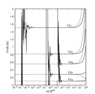
Figure 2: The finite functions for the triply massive triangle graph with $s_{12}=1,~{}~{}p_{1}^{2}=0.2$ as a function of $\Delta_{3}/\Delta_{3}^{{\rm max}}$ where $\Delta_{3}^{{\rm max}}=-(s_{12}-p_{1}^{2})^{2}$. The functions have been evaluated using double precision Fortran. The dashed lines show the approximate form for the function in the limit $\Delta_{3}\to 0$, retaining only the first term of the Taylor expansion.

By expanding as a series in $\Delta_{3}$, these functions can be evaluated near the singularity with arbitrary precision. For example,

$$\lim_{\Delta_{3}\rightarrow 0}{\rm I}_{3}[x_{3}^{2}] = \frac{(s_{12}+p_{1}^{2}-p_{2}^{2})}{3s_{12}(s_{12}-p_{1}^{2}-p_{2}^{2})}-\frac{2p_{1}^{4}}{3s_{12}(s_{12}-p_{1}^{2}-p_{2}^{2})^{2}}\log\left(\frac{s_{12}}{p_{1}^{2}}\right)$$

$$\qquad+\frac{(3s_{12}-3p_{1}^{2}+p_{2}^{2})}{6s_{12}(s_{12}-p_{1}^{2}-p_{2}^{2})}\log\left(\frac{s_{12}}{p_{2}^{2}}\right).$$

To illustrate this, fig. 2 shows the various functions at a specific phase space point, $s_{12}=1,~{}~{}p_{1}^{2}=0.2$ and letting $p_{2}^{2}$ vary in such a way that $\Delta_{3}\to 0$. This corresponds to $p_{2}^{2}\to 0.135$. We see that as this limit is approached, the numerical evaluation of the function using double precision (an intrinsic numerical precision, $acc$, of roughly $10^{-14}$) becomes uncertain. For this particular phase space point, functions with a single Gram determinant in the denominator (${\rm Lc}_{1}$) remain stable until $\Delta_{3}/\Delta_{3}^{{\rm max}}\sim 10^{-9}$ while those with more powers of the Gram determinant break down correspondingly sooner - at $\Delta_{3}/\Delta_{3}^{{\rm max}}\sim 10^{-6}$ for ${\rm Lc}_{2}$ and ${\rm Lc}_{3}$ and $\Delta_{3}/\Delta_{3}^{{\rm max}}\sim 10^{-4}$ for ${\rm Lc}_{4}$ and ${\rm Lc}_{5}$. In general, numerical problems typically occur when $\Delta_{3}/\Delta_{3}^{{\rm max}}\sim(acc)^{1/N}$ where $N$ is the number of Gram determinants in the denominator of the function. Other phase space points yield a similar behaviour.

The unstable points represent a rather small proportion of the allowed phase space. However, problems may arise using adaptive Monte Carlo methods such as VEGAS [19] where the phase space is preferentially sampled where the matrix elements are large. Finding an anomalously high value for the matrix elements in a region of instability would cause the Monte Carlo integration to focus on that region giving unpredictable results.

Of course, these instabilities could be handled by a brute force increase in numerical precision. While possible, this has the disadvantage of producing significantly slower code, and, since in all cases, the approximate form obtained by making a Taylor expansion about $\Delta_{3}=0$ and keeping only the constant term works well where the numerical instabilities begin, this is not an attractive solution. In fact, the approximation is reliable for $\Delta_{3}<10^{-3}\Delta_{3}^{{\rm max}}$. Explicit forms for the approximations are collected in Appendix C.

3.1.2 Scalar integrals in higher dimensions

We now turn to the scalar triangle integrals in higher dimensions. They appear in the $g_{\mu\nu}$ part of the general Lorentz structure and recursively in the determination of ${\rm I}_{4}^{D=4-2\epsilon}[x_{i}...x_{l}]$. Unlike the triangle in four dimensions, these integrals are ultraviolet divergent due to the presence of the various pinchings - bubble integrals. A function that can usefully be used as a building block of matrix element calculations, must be finite as both $\Delta_{3}\to 0$ and $\epsilon\to 0$ and we must first isolate the poles in $\epsilon$. Although equation (2.4) suggests that the ultraviolet pole structure involves $\Delta_{3}$, this is easily shown not to be the case. Adding terms proportional to,

$$\frac{1}{2}\left(\hat{\Delta}_{3}-\sum_{m=1}^{3}\hat{\gamma}_{m}\alpha_{m}\right)\frac{1}{\alpha_{2}}\hat{\rm I}^{(2)}_{2}[1]=0,$$

to equation (2.4) for $n=3$, $D=4-2\epsilon$ we see,

$$\hat{\rm I}^{D=6-2\epsilon}_{3}[1]=-\frac{1}{(1-\epsilon)}\frac{1}{\hat{\Delta}_{3}}\left(\hat{\rm I}_{3}[1]+\frac{1}{2}\sum_{m=1}^{3}\frac{\gamma_{m}}{\prod\alpha}\left({\rm I}_{2}^{(m)}[1]-{\rm I}_{2}^{(2)}[1]\right)+\frac{\hat{\Delta}_{3}}{2\prod\alpha}{\rm I}_{2}^{(2)}[1]\right),$$

where the divergence as $\epsilon\to 0$ lies exclusively in the last term. Reinserting the factors of $\alpha$ and the definition of ${\rm I}_{2}[1]$ in $D=4-2\epsilon$ dimensions we find,

$${\rm I}^{D=6-2\epsilon}_{3}[1]={\rm Lc}_{1S}(p_{1},p_{2})-\frac{1}{2}\left(\frac{(-s_{12})^{-\epsilon}}{\epsilon}+3\right)c_{\Gamma},$$ (3.10)

where,

$${\rm Lc}_{1S}(p_{1},p_{2}) = \frac{1}{2\Delta_{3}}\Biggl{(}2p_{1}^{2}p_{2}^{2}s_{12}{\rm I}_{3}[1]-p_{1}^{2}(s_{12}+p_{2}^{2}-p_{1}^{2})\log\left(\frac{s_{12}}{p_{1}^{2}}\right)$$ (3.11)

$$\qquad-p_{2}^{2}(s_{12}+p_{1}^{2}-p_{2}^{2})\log\left(\frac{s_{12}}{p_{2}^{2}}\right)\Biggr{)}$$

$$= \frac{1}{2}\left(p_{1}^{2}{\rm I}_{3}[x_{1}]+p_{2}^{2}{\rm I}_{3}[x_{3}]\right).$$

In a similar fashion, the $\epsilon$ pole structure can be removed from the triangle scalar integral in $D=8-2\epsilon$ and $D=10-2\epsilon$ dimensions yielding two more functions that are finite as both $\Delta_{3}\to 0$ and $\epsilon\to 0$. Explicitly we find,

$${\rm I}^{D=8-2\epsilon}_{3}[1] = {\rm Lc}_{2S}(p_{1},p_{2})-\frac{(p_{1}^{2}+p_{2}^{2}+s_{12})}{24}\left(\frac{(-s_{12})^{-\epsilon}}{\epsilon}+\frac{19}{6}\right)c_{\Gamma},$$ (3.12)

$${\rm I}^{D=10-2\epsilon}_{3}[1] = {\rm Lc}_{3S}(p_{1},p_{2})-\frac{(p_{1}^{4}+p_{2}^{4}+s_{12}^{2}+p_{1}^{2}p_{2}^{2}+p_{1}^{2}s_{12}+p_{2}^{2}s_{12})}{360}\left(\frac{(-s_{12})^{-\epsilon}}{\epsilon}+\frac{17}{5}\right)c_{\Gamma},$$

where the finite functions are defined by,

$${\rm Lc}_{2S}(p_{1},p_{2}) = \frac{1}{4\Delta_{3}}\left(2p_{1}^{2}p_{2}^{2}s_{12}{\rm Lc}_{1S}(p_{1},p_{2})-\frac{1}{6}\left(p_{1}^{4}(s_{12}+p_{2}^{2}-p_{1}^{2})\log\left(\frac{s_{12}}{p_{1}^{2}}\right)\right.\right.$$ (3.14)

$$\qquad\left.\left.+p_{2}^{4}(s_{12}+p_{1}^{2}-p_{2}^{2})\log\left(\frac{s_{12}}{p_{2}^{2}}\right)+2p_{1}^{2}p_{2}^{2}s_{12}\right)\right),$$

$${\rm Lc}_{3S}(p_{1},p_{2}) = \frac{1}{6\Delta_{3}}\Biggl{(}2p_{1}^{2}p_{2}^{2}s_{12}{\rm Lc}_{2S}(p_{1},p_{2})-\frac{1}{60}\Biggl{(}p_{1}^{6}(s_{12}+p_{2}^{2}-p_{1}^{2})\log\left(\frac{s_{12}}{p_{1}^{2}}\right)$$ (3.15)

$$\qquad+p_{2}^{6}(s_{12}+p_{1}^{2}-p_{2}^{2})\log\left(\frac{s_{12}}{p_{2}^{2}}\right)+\frac{p_{1}^{2}p_{2}^{2}s_{12}}{2}(p_{1}^{2}+p_{2}^{2}+s_{12})\Biggr{)}\Biggr{)}.$$

Although these functions have been obtained via equation (2.4), they are still related to derivatives of the basic scalar integral in $D=4-2\epsilon$, and are therefore finite in the $\Delta_{3}\to 0$ limit. We can see this by examining the same phase space point as before, $s_{12}=1,~{}~{}p_{1}^{2}=0.2$ and varying $\Delta_{3}$. As expected, the ${\rm Lc}_{nS}$ show a similar behaviour to the ${\rm Lc}_{n}$ functions - numerically breaking down at larger and larger values of $\Delta_{3}$ as the number of Gram determinants increases, and being well described by the first term in the Taylor expansion as this happens. For completeness, we collect the limiting approximations in Appendix C.

3.1.3 Tensor integrals in higher dimensions

For triangle loop integrals with three loop momenta in the numerator, it is also necessary to know the $D=6-2\epsilon$ integral with a single Feynman parameter in the numerator. Rather than differentiating the ultraviolet divergent ${\rm I}_{3}^{D=6-2\epsilon}[1]$, we can evaluate it in terms of the $D=4-2\epsilon$ tensor integrals of section 3.1.1. Using (2.6) for $D=4-2\epsilon$, we see that,

$$\hat{\rm I}_{3}[a_{1}a_{j}]+\hat{\rm I}_{3}[a_{3}a_{j}] = \frac{1}{2}\Biggl{(}-(3-2\epsilon)(\hat{\gamma}_{1}+\hat{\gamma}_{3})\hat{\rm I}_{3}^{D=6-2\epsilon}[a_{j}]+(\eta_{1j}+\eta_{3j})\hat{\rm I}_{3}^{D=6-2\epsilon}[1]$$

$$\qquad-\sum_{m=1}^{3}(\eta_{1m}+\eta_{3m})\hat{\rm I}_{2}^{(m)}[a_{j}]\Biggr{)},$$

which, for $j=1,3,$ simplifies using,

$$\eta_{1j}+\eta_{3j}=0.$$

The same equation simplifies the sum over bubble pinchings so that only $m=2$ contributes, while $\hat{\gamma}_{1}+\hat{\gamma}_{3}=2\alpha_{2}$. Restoring the factors of $\alpha$ and using,

$${\rm I}_{2}^{(2)}[x_{1}]={\rm I}_{2}^{(2)}[x_{3}]=\frac{1}{2}\left(\frac{(-s_{12})^{-\epsilon}}{\epsilon}+2\right)c_{\Gamma},$$

yields,

$${\rm I}_{3}^{6-2\epsilon}[x_{j}]=\frac{1}{3}\Biggl{(}p_{1}^{2}{\rm I}_{3}[x_{1}x_{j}]+p_{2}^{2}{\rm I}_{3}[x_{3}x_{j}]\Biggr{)}-\frac{1}{6}\left(\frac{(-s_{12})^{-\epsilon}}{\epsilon}+\frac{8}{3}\right)c_{\Gamma}.$$ (3.16)

Later, we will see that constructing the tensor integrals for box graphs can also generate ${\rm I}_{3}^{6-2\epsilon}[x_{j}]$ and higher dimensional triangle integrals with more parameters in the numerator. In each case, we use similar tricks with equations (2.7–2.10) to rewrite them in terms of the four dimensional integrals with the ultraviolet pole made explicit.

3.2 The two-mass triangle

We will also be interested in triangle graphs where one or more of the external momenta is lightlike. Here, we first focus on the case, $p_{2}^{2}\to 0$. In $D=4-2\epsilon$ dimensions, we have the well known result,

$$\hat{\rm I}_{3}^{2m}[1]=\frac{c_{\Gamma}}{\epsilon^{2}}\left(\frac{(\alpha_{1}\alpha_{3})^{\epsilon}-(\alpha_{1}\alpha_{2})^{\epsilon}}{\alpha_{3}-\alpha_{2}}\right),$$ (3.17)

where the superscript indicates that only two of the three legs are massive. For this choice of kinematics,

$$\alpha_{1}\alpha_{2}p_{1}^{2}=-1,\qquad\alpha_{1}\alpha_{3}s_{12}=-1,$$

and

$$\hat{\Delta}_{3}=-(\alpha_{3}-\alpha_{2})^{2},$$

so that the singular limit is $\alpha_{3}\to\alpha_{2}$. Because $\hat{\Delta}_{3}$ makes no reference to $\alpha_{1}$, $\eta_{ij}$ contains a row of zeroes,

$$\eta_{ij}=\left(\begin{array}[]{rrrr}0&0&0\\ 0&-1&1\\ 0&1&-1\end{array}\right),$$

and therefore $N_{3}=0$. Consequently, care is needed in applying the equations of section 2. In addition, since the scalar integral for three massive legs is finite (and the results in the preceding subsections have been explicitly derived in $D=4$), one cannot just set $p_{2}^{2}\to 0$.

In fact, it is easiest just to bypass the problem and generate the whole tensor structure by direct differentiation of the scalar integral with respect to $\alpha_{3}$ and $\alpha_{1}$. It is easy to see that,

$$\hat{\rm I}_{3}^{2m}[a_{3}^{n}]\sim A\hat{\rm I}_{3}^{2m}[1]+B\frac{(\alpha_{1}\alpha_{3})^{\epsilon}}{\epsilon}+C\log\left(\frac{\alpha_{3}}{\alpha_{2}}\right)+D,$$

where $A,B,C$ and $D$ are polynomials in $1/\alpha_{3}$ and $1/(\alpha_{3}-\alpha_{2})$. Unlike the all massive case discussed before, the scalar integral is singular as $\epsilon\to 0$. As a general rule it is not necessary to be particularly careful with double poles in $\epsilon$, since they must either cancel or form the infrared poles of real matrix elements. However, it is possible for the integrals to be multiplied by factors of $\epsilon$ - from expanding factors of dimension - and the resulting logarithms should occur in combinations that are finite as $\alpha_{3}\to\alpha_{2}$. It is easy to see that,

$$\epsilon\times\hat{\rm I}_{3}^{2m}[1]=\frac{\log\left(\frac{\alpha_{3}}{\alpha_{2}}\right)}{\alpha_{3}-\alpha_{2}}+{\cal O}(\epsilon),$$

is finite. So, to tie the logarithms and constants together in combinations that are well behaved in the $\alpha_{3}\to\alpha_{2}$ limit, we use the fact that derivatives of this function are also well behaved, and introduce the functions,

$${\rm Lc}_{n}^{2m}(p_{1},p_{2})=-\lim_{\epsilon\rightarrow 0}\left(\epsilon\times{\rm I}^{2m}_{3}[x_{3}^{n-1}]\right),$$ (3.18)

for $n=1,\ldots,4$. In terms of invariants,

$${\rm Lc}_{n}^{2m}(p_{1},p_{2})=-\left(\frac{p_{1}^{2}{\rm Lc}_{n-1}^{2m}(p_{1},p_{2})-\frac{1}{n-1}}{s_{12}-p_{1}^{2}}\right),\qquad n\geq 2$$ (3.19)

with,

$${\rm Lc}_{1}^{2m}(p_{1},p_{2})=\frac{\log\left(\frac{s_{12}}{p_{1}^{2}}\right)}{s_{12}-p_{1}^{2}},\qquad{\rm Lc}_{0}^{2m}(p_{1},p_{2})=\log\left(\frac{s_{12}}{p_{1}^{2}}\right).$$ (3.20)

These functions, or functions closely related to them, have appeared in next-to-leading order matrix element calculations [15, 16, 17, 5]. The explicit forms for ${\rm I}_{3}^{2m}[x_{i}x_{j}]$ appearing in the momentum expansion are well known and are collected in Appendix A.

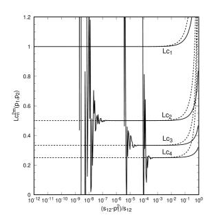
Figure 3: The finite functions for the triangle graph with two external masses with $s_{12}=1$ evaluated in double precision Fortran as a function of $(s_{12}-p_{1}^{2})/s_{12}$. The dashed lines show the approximate form for the function in the limit $p_{1}^{2}\to s_{12}$, retaining only the first term of the Taylor expansion.

Although these functions are rather simple, they still contain numerical instabilities as $p_{1}^{2}\to s_{12}$. This can be seen in Fig. 3 where we show ${\rm Lc}_{n}^{2m}$ for the specific phase space point $s_{12}=1$ and let $p_{1}^{2}$ approach $s_{12}$. While a single inverse powers of $(s_{12}-p_{1}^{2})$ is handled correctly, higher powers cause problems. As can be seen from the figure, a suitable approximation is obtained by the first term in the Taylor expansion,

$$\lim_{p_{1}^{2}\to s_{12}}{\rm Lc}_{n}^{2m}(p_{1},p_{2})=\frac{1}{np_{1}^{2}},$$

for $n\geq 1$.

The other configuration of triangle graph that appears is where two of the momenta are lightlike, $p_{1}^{2}=p_{2}^{2}=0$. Once again, the tensor structure can be generated by differentiation or canonical Passarino-Veltman reduction. Here, there is only one scale in the problem so there can be no logarithms and it is neither possible nor necessary to introduce well behaved functions. The explicit forms for the Feynman parameter integrals appearing in the momentum expansion are well known and for the sake of completeness are given in Appendix A.

This concludes our discussion of triangle graphs. For the case of three massive external legs (and internal masses set equal to zero) the four dimensional tensor integrals are finite as $\epsilon\to 0$ and are given by the functions ${\rm Lc}_{0\ldots 5}(p_{1},p_{2})$ defined in (3.1,3.4,3.6–3.9), while the ultraviolet divergent part $g_{\mu\nu}$ part, ${\rm I}_{3}^{D=6-2\epsilon}[1]$ is expressed in terms of a similar function (${\rm Lc}_{1S}$) with the pole isolated (3.11). For the tensor structure in the simpler case with one lightlike leg, it is useful to group the logarithms and constants using the functions ${\rm Lc}_{1\ldots 4}^{2m}(p_{1},p_{2})$ (3.20, 3.19).

For the more general case where the internal masses are non-zero, the same procedure can be utilised. The matrix $\eta$ has slightly more entries and there are more scales in the problem. However, the grouping together of triangle graphs and bubble integrals into functions well behaved in the $\Delta_{3}\to 0$ limit and the isolation of the ultraviolet singularities can be made explicit in the same way.

4 Four point integrals

For one-loop corrections to five parton scattering, box graphs with at most one external leg occur. However, for processes involving a massive vector boson and four massless partons, we can obtain box graphs with a second massive external leg by pinching together two of the partons. There are two distinct configurations according to the positions of the massive legs; the adjacent box graph and the opposite box graph. The box graph is shown in fig. 4 for outgoing momenta $p_{1}$, $p_{2}$ and $p_{3}$. Throughout this section, we will assume that $(p_{1}+p_{2}+p_{3})^{2}=s_{123}\neq 0$. In the adjacent two mass case, $p_{2}^{2}=p_{3}^{2}=0$ and $p_{1}^{2}\neq 0$, while for the opposite box, $p_{1}^{2}=p_{3}^{2}=0$ and $p_{2}^{2}\neq 0$. Unfortunately, the raw scalar integrals for these two cases behave rather differently. The adjacent box is finite in the limit that $\Delta_{4}\to 0$, while the opposite box diverges as $\Delta_{4}\to 0$. In this section, we work through these two configurations and rewrite the tensor integrals in terms of well behaved functions and explicit poles in $\epsilon$.

Figure 4: The box graph and each of the four pinchings obtained by omitting the internal line associated with $\alpha_{m}$ for $m=1,2,3$ and 4.

4.1 The adjacent two-mass box

We first consider the adjacent box with $p_{2}^{2}=p_{3}^{2}=0$ and all internal masses equal to zero. As in the triangle case, we systematically eliminate one of the momenta, $p_{4}=-(p_{1}+p_{2}+p_{3})$, and one of the Feynman parameters, $x_{3}=1-x_{1}-x_{2}-x_{4}$, so that,

$${\cal P}^{\mu}=-(1-x_{1})p_{12}^{\mu}+x_{2}p_{2}^{\mu}-x_{4}p_{3}^{\mu}.$$

The related integrals with $p_{3}^{2}\neq 0$ and $p_{1}^{2}=0$ are obtained by $p_{1}\leftrightarrow p_{3}$ (and the indices $i$ and $j$ in $\alpha_{i}$ and $\eta_{ij}$ transform as $1\leftrightarrow 4$ and $2\leftrightarrow 3$).

For this kinematic configuration, the $\alpha$ parameters are defined by,

$$\begin{array}[]{rr}\alpha_{1}\alpha_{4}\,s_{123}=-1,&\alpha_{1}\alpha_{2}\,p_{1}^{2}=-1\\ \alpha_{1}\alpha_{3}\,s_{12}=-1,&\alpha_{2}\alpha_{4}\,s_{23}=-1,\end{array}$$

while,

$$\begin{array}[]{lr}\eta_{ij}=\left(\begin{array}[]{rrrr}0&0&1&0\\ 0&0&-1&1\\ 1&-1&2&-1\\ 0&1&-1&0\end{array}\right),&N_{4}=\frac{1}{2},\end{array}$$

and,

$$\Delta_{4}=2s_{23}\left((s_{123}-s_{12})(s_{12}-p_{1}^{2})-s_{12}s_{23}\right).$$

The coefficients $\gamma_{i}$ always appear in the following combinations which are directly related to the conventional variables,

$$\frac{\gamma_{i}}{\prod_{j=1}^{4}\alpha_{j}}=\left\{\begin{array}[]{ll}-s_{23}&i=1\\ s_{123}-s_{12}&i=2\\ s_{123}+p_{1}^{2}-s_{23}-{2p_{1}^{2}s_{123}\over s_{12}}&i=3\\ p_{1}^{2}-s_{12}&i=4\\ \end{array}\right..$$

The scalar integral in $D=4-2\epsilon$ can be written [4, 8],

$$\hat{\rm I}_{4}[1]=\frac{c_{\Gamma}}{\epsilon^{2}}\left((\alpha_{2}\alpha_{4})^{\epsilon}+2(\alpha_{1}\alpha_{3})^{\epsilon}-(\alpha_{1}\alpha_{2})^{\epsilon}-(\alpha_{1}\alpha_{4})^{\epsilon}\right)+2{\rm Ld}_{0}(p_{1},p_{2},p_{3})+{\cal O}(\epsilon),$$ (4.1)

where,

$${\rm Ld}_{0}(p_{1},p_{2},p_{3})={\rm Li_{2}}\left(1-\frac{\alpha_{4}}{\alpha_{3}}\right)-{\rm Li_{2}}\left(1-\frac{\alpha_{3}}{\alpha_{2}}\right)+\frac{1}{2}\log\left(\frac{\alpha_{2}\alpha_{4}}{\alpha_{3}^{2}}\right)\log\left(\frac{\alpha_{1}}{\alpha_{2}}\right).$$ (4.2)

In constructing the tensor integrals in $D=4-2\epsilon$, we see from equations (2.7–2.10) that the box integral in higher dimensions is needed. In fact, in $D=6-2\epsilon$, the box integral is infrared and ultraviolet finite. This can be seen by inspection of equation (2.4) and noting that the pinchings with $m=1,2$ and 4 in the expression,

$$\hat{\rm I}_{4}[1]+\sum_{m=1}^{4}\hat{\gamma}_{m}\hat{\rm I}_{3}^{(m)}[1],$$

are proportional to $1/\epsilon^{2}$ and, when combined with the appropriate $\hat{\gamma}$ factor, precisely cancel with the pole structure of the box integral. The final pinching ($m=3$) corresponds to the triangle graph with three massive external legs which is itself finite. Altogether, we find that the adjacent box integral in $D=6$ is,

$${\rm I}_{4}^{D=6}[1] = -\frac{2s_{12}s_{23}}{\Delta_{4}}\left({\rm Ld}_{0}(p_{1},p_{2},p_{3})+\frac{1}{2}\left(s_{123}+p_{1}^{2}-s_{23}-\frac{2p_{1}^{2}s_{123}}{s_{12}}\right){\rm Lc}_{0}(p_{1},p_{23})\right)$$ (4.3)

$$\equiv {\rm Ld}_{1S}(p_{1},p_{2},p_{3}),$$

where ${\rm Lc}_{0}(p_{1},p_{23})={\rm I}_{3}[1]$ is defined in equation (3.1). Because of the finiteness properties of the three mass triangle, we will find repeatedly that the $m=3$ pinching should be treated differently from the other three.

4.1.1 Scalar integrals in higher dimensions

For higher dimensions, we just reuse equation (2.4), noting that the triangle pinchings in $D=6-2\epsilon$ reintroduce ultraviolet poles. These can easily be isolated by adding and subtracting combinations of scalar integrals as in section 3.1.2. Explicitly,

$${\rm I}_{4}^{D=8-2\epsilon}[1] = {\rm Ld}_{2S}(p_{1},p_{2},p_{3})+\frac{c_{\Gamma}}{6}\left(\frac{(-s_{123})^{-\epsilon}}{\epsilon}+\frac{11}{3}\right),$$ (4.4)

$${\rm I}_{4}^{D=10-2\epsilon}[1] = {\rm Ld}_{3S}(p_{1},p_{2},p_{3})+\frac{c_{\Gamma}(s_{123}+s_{12}+s_{23}+p_{1}^{2})}{120}\left(\frac{(-s_{123})^{-\epsilon}}{\epsilon}+\frac{107}{30}\right),$$ (4.5)

$${\rm I}_{4}^{D=12-2\epsilon}[1] = {\rm Ld}_{4S}(p_{1},p_{2},p_{3})+\frac{c_{\Gamma}P}{2520}\left(\frac{(-s_{123})^{-\epsilon}}{\epsilon}+\frac{129}{35}\right),$$ (4.6)

where,

$$P=s_{123}^{2}+s_{12}^{2}+s_{23}^{2}+p_{1}^{4}+s_{123}s_{12}+s_{123}s_{23}+s_{123}p_{1}^{2}+s_{12}p_{1}^{2}+s_{23}p_{1}^{2}+\frac{s_{12}s_{23}}{2}.$$

The finite parts of the higher dimension boxes are given by,

$${\rm Ld}_{2S}(p_{1},p_{2},p_{3}) = -\frac{s_{12}s_{23}}{3\Delta_{4}}\Biggl{(}s_{12}s_{23}{\rm Ld}_{1S}(p_{1},p_{2},p_{3})$$ (4.7)

$$+\left(s_{123}+p_{1}^{2}-s_{23}-\frac{2p_{1}^{2}s_{123}}{s_{12}}\right){\rm Lc}_{1S}(p_{1},p_{23})$$

$$+\frac{s_{23}}{2}\log\left(\frac{s_{123}}{s_{23}}\right)+s_{12}\log\left(\frac{s_{123}}{s_{12}}\right)-\frac{p_{1}^{2}}{2}\log\left(\frac{s_{123}}{p_{1}^{2}}\right)\Biggr{)},$$

$${\rm Ld}_{3S}(p_{1},p_{2},p_{3}) = -\frac{s_{12}s_{23}}{5\Delta_{4}}\Biggl{(}s_{12}s_{23}{\rm Ld}_{2S}(p_{1},p_{2},p_{3})$$ (4.8)

$$+\left(s_{123}+p_{1}^{2}-s_{23}-\frac{2p_{1}^{2}s_{123}}{s_{12}}\right){\rm Lc}_{2S}(p_{1},p_{23})$$

$$+\frac{s_{23}^{2}}{24}\log\left(\frac{s_{123}}{s_{23}}\right)+\frac{s_{12}^{2}}{12}\log\left(\frac{s_{123}}{s_{12}}\right)-\frac{p_{1}^{4}}{24}\log\left(\frac{s_{123}}{p_{1}^{2}}\right)+\frac{s_{12}s_{23}}{12}\Biggr{)},$$

$${\rm Ld}_{4S}(p_{1},p_{2},p_{3}) = -\frac{s_{12}s_{23}}{7\Delta_{4}}\Biggl{(}s_{12}s_{23}{\rm Ld}_{3S}(p_{1},p_{2},p_{3})$$ (4.9)

$$+\left(s_{123}+p_{1}^{2}-s_{23}-\frac{2p_{1}^{2}s_{123}}{s_{12}}\right){\rm Lc}_{3S}(p_{1},p_{23})$$

$$+\frac{s_{23}^{3}}{360}\log\left(\frac{s_{123}}{s_{23}}\right)+\frac{s_{12}^{3}}{180}\log\left(\frac{s_{123}}{s_{12}}\right)-\frac{p_{1}^{6}}{360}\log\left(\frac{s_{123}}{p_{1}^{2}}\right)$$

$$+\frac{s_{12}s_{23}(s_{123}+s_{12}+s_{23}+p_{1}^{2})}{720}\Biggr{)}.$$

The $D=6-2\epsilon$ and $D=8-2\epsilon$ box integrals explicitly appear in the momentum space tensor structure with one and two factors of $g_{\mu\nu}$ respectively. All of these integrals appear either directly or indirectly in the tensor box integrals of equations (2.7–2.10).

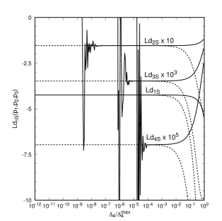
Figure 5: The finite functions for the one mass box graph as a function of $\Delta_{4}/\Delta_{4}^{{\rm max}}$ where $\Delta_{4}^{{\rm max}}=2s_{12}s_{23}(s_{123}-s_{12}-s_{23})$. The phase space point is $s_{123}=1$, $s_{12}=0.4$, $s_{23}=0.08$ and $p_{1}^{2}$ altered so the limit is approached and the functions have been evaluated in double precision Fortran. The dashed lines show the approximate form for the function in the limit $\Delta_{4}\to 0$, retaining only the first term of the Taylor expansion as given in Appendix C.

Once again, all of these functions are well behaved as $\Delta_{4}\to 0$ and group a variety of dilogarithms, logarithms and constants together in a non-trivial way. This is shown in Fig. 5 for a particular point in phase space; $s_{123}=1$, $s_{12}=0.4$, $s_{23}=0.08$ with $p_{1}^{2}$ varying so the $\Delta_{4}\to 0$ limit is approached. We see that although ${\rm Ld}_{1S}$, with a single inverse power of the Gram determinant, is numerically stable, the functions with more powers of Gram determinant in the denominator break down at much larger values of $\Delta_{4}$. In all cases, the function is well approximated by the first term of the Taylor expansion provided $\Delta_{4}<10^{-4}\Delta_{4}^{{\rm max}}$. These approximations are collected in Appendix C.

4.1.2 Tensor integrals

Armed with the integrals in $D>4$, we return to the tensor integrals and use equations (2.7–2.10) as the starting point. Rewriting equation (2.7) for $n=4$, $D=4-2\epsilon$ and noting that we have eliminated $x_{3}$ so that $i=1,2$ and 4 only, we have,

$${\rm I}_{4}[x_{i}]=-\gamma_{i}{\rm I}_{4}^{D=6}[1]-\sum_{m=1}^{4}\eta_{im}\alpha_{i}\alpha_{m}{\rm I}_{3}^{(m)}[1].$$

The factor $\alpha_{i}\alpha_{m}$ multiplying the triangle pinchings will always produce a factor of $1/s$. For triangle graphs with at least one massless leg (pinchings $m=1,2$ and 4), the contribution is $\sim 1/\epsilon^{2}$ and will combine with similar poles from other Feynman diagrams. On the other hand, the $m=3$ pinching (corresponding to the triangle graph with momenta $p_{1}$ and $p_{23}$ flowing outwards) is finite and, provided the value of $s$ is related kinematically to that triangle pinching, there may be a possibility of cancellation with other triangle Feynman graphs. However, for the case $i=1$ and $m=3$, the associated invariant mass is $s_{12}$. This term cannot combine with any other naturally generated triangle graph with the same kinematics. Therefore, we group this term with the box integral, by adding and subtracting,

$$\sum_{m=1}^{4}\eta_{im}\alpha_{i}\alpha_{m}{\rm I}_{3}^{(3)}[1]=\gamma_{i}{\rm I}_{3}^{(3)}[1],$$

so that,

$${\rm I}_{4}[x_{i}]=\gamma_{i}{\rm Ld}_{1}(p_{1},p_{2},p_{3})-\sum_{m=1}^{4}\eta_{im}\alpha_{i}\alpha_{m}\left({\rm I}_{3}^{(m)}[1]-{\rm I}_{3}^{(3)}[1]\right),$$ (4.10)

with,

$${\rm Ld}_{1}(p_{1},p_{2},p_{3})=-\left({\rm I}_{4}^{D=6}[1]+{\rm I}_{3}^{(3)}[1]\right).$$ (4.11)

The only non-zero entries in $\eta_{im}$ for $i\neq 3$ and $m\neq 3$ are $i=2,~{}m=4$ or $i=4,~{}m=2$ corresponding to $\alpha_{i}\alpha_{m}=-1/s_{23}$ which is appropriate for ${\rm I}_{3}^{(3)}[1]$.

For integrals with more Feynman parameters it is convenient to introduce the following functions,

$${\rm Ld}_{ni_{1}\ldots i_{n-1}}(p_{1},p_{2},p_{3})=-\biggl{\{}n{\rm I}_{4}^{D=6}[x_{i_{1}}\ldots x_{i_{n-1}}]+{\rm I}_{3}^{(3)}[x_{i_{1}}\ldots x_{i_{n-1}}]\biggr{\}},$$ (4.12)

for $n=2,3$ and 4. Suppressing the arguments of ${\rm Ld}_{n}$, and using equations (2.8-2.10), we find,

$${\rm I}_{4}[x_{i}x_{j}] = \gamma_{i}{\rm Ld}_{2j}-\eta_{ij}\alpha_{i}\alpha_{j}\biggl{\{}{\rm Ld}_{1}+{\rm I}_{3}^{(3)}[1]\biggr{\}}-\sum_{m=1}^{4}\eta_{im}\alpha_{i}\alpha_{m}\biggl{\{}{\rm I}_{3}^{(m)}[x_{j}]-{\rm I}_{3}^{(3)}[x_{j}]\biggr{\}},$$ (4.13)

$${\rm I}_{4}[x_{i}x_{j}x_{k}] = \gamma_{i}{\rm Ld}_{3jk}-\frac{1}{2}\eta_{ij}\alpha_{i}\alpha_{j}\biggl{\{}{\rm Ld}_{2k}+{\rm I}_{3}^{(3)}[x_{k}]\biggr{\}}-\frac{1}{2}\eta_{ik}\alpha_{i}\alpha_{k}\biggl{\{}{\rm Ld}_{2j}+{\rm I}_{3}^{(3)}[x_{j}]\biggr{\}}$$ (4.14)

$$\quad-\sum_{m=1}^{4}\eta_{im}\alpha_{i}\alpha_{m}\biggl{\{}{\rm I}_{3}^{(m)}[x_{j}x_{k}]-{\rm I}_{3}^{(3)}[x_{j}x_{k}]\biggr{\}},$$

$${\rm I}_{4}[x_{i}x_{j}x_{k}x_{l}] = \gamma_{i}{\rm Ld}_{4jkl}-\frac{1}{3}\eta_{ij}\alpha_{i}\alpha_{j}\biggl{\{}{\rm Ld}_{3kl}+{\rm I}_{3}^{(3)}[x_{k}x_{l}]\biggr{\}}-\frac{1}{3}\eta_{ik}\alpha_{i}\alpha_{k}\biggl{\{}{\rm Ld}_{3jl}+{\rm I}_{3}^{(3)}[x_{j}x_{l}]\biggr{\}}$$

$$-\frac{1}{3}\eta_{il}\alpha_{i}\alpha_{l}\biggl{\{}{\rm Ld}_{3jk}+{\rm I}_{3}^{(3)}[x_{j}x_{k}]\biggr{\}}-\sum_{m=1}^{4}\eta_{im}\alpha_{i}\alpha_{m}\biggl{\{}{\rm I}_{3}^{(m)}[x_{j}x_{k}x_{l}]-{\rm I}_{3}^{(3)}[x_{j}x_{k}x_{l}]\biggr{\}}.$$

Since we have systematically eliminated $x_{3}$ using the delta function, $i,~{}j,~{}k$ and $l$ run over $1,~{}2$ and 4. This guarantees that the coefficients of the form $\eta_{ij}\alpha_{i}\alpha_{j}$ are only non-zero for $i=2$ and $j=4$ (or vice-versa). In these cases, $\eta_{24}\alpha_{2}\alpha_{4}=-1/s_{23}$, which is again appropriate for the $m=3$ pinching to form a completely massive triangle, ${\rm I}_{3}^{(3)}[1]$. Altogether, equations (4.10,4.13–4.1.2) are sufficient to completely describe the tensor structure of the adjacent box.

However, in order to determine the ${\rm Ld}_{ni_{1}\ldots i_{n-1}}$ combinations, we need tensor integrals for $D=6-2\epsilon$ dimensional box graphs with two or more Feynman parameters. These can be obtained from equation (2.8) once the $D=6-2\epsilon$ box integral with a single Feynman parameter, ${\rm I}_{4}^{D=6-2\epsilon}[x_{i}]$ is known. This can be derived by differentiating (2.2) which indicates that ${\rm I}_{4}^{D=6-2\epsilon}[x_{i}]$ is also finite as $\epsilon\to 0$. To see this, we reuse equation (2.7) and our usual trick of adding and subtracting combinations of the $m=3$ pinching in $D=6-2\epsilon$,

$${\rm I}_{4}^{D=6-2\epsilon}[x_{i}] = \gamma_{i}\left(-(3-2\epsilon){\rm I}_{4}^{D=8-2\epsilon}[1]-{\rm I}_{3}^{D=6-2\epsilon(3)}[1]\right)$$

$$\qquad-\sum_{m=1}^{4}\eta_{im}\alpha_{i}\alpha_{m}\left({\rm I}_{3}^{D=6-2\epsilon(m)}[1]-{\rm I}_{3}^{D=6-2\epsilon(3)}[1]\right).$$

Both brackets are separately finite. First, the divergent part of ${\rm I}_{4}^{D=8-2\epsilon}[1]$ precisely cancels against that of ${\rm I}_{3}^{D=6-2\epsilon(3)}[1]$. Second, all triangles in $D=6-2\epsilon$ dimensions have $1/\epsilon$ poles and the difference of any two, is either zero or a log. Further differentiation does not change the finiteness properties of the ${\rm I}_{4}^{D=6-2\epsilon}$ tensor integrals.

The ${\rm Ld}_{ni_{1}\ldots i_{n-1}}$ combinations are also well behaved in certain kinematic limits. For example, ${\rm I}_{4}^{D=6}[1]$ and ${\rm I}_{3}^{(3)}[1]$ are finite as $s_{12}\to 0$ or $s_{23}\to 0$. Just as differentiating functions which are finite as $\epsilon\to 0$ does not introduce poles in $\epsilon$, neither can it introduce poles in the kinematic invariants $s_{12}$ or $s_{23}$. As an example, consider the function ${\rm Ld}_{24}$ given by,

$${\rm Ld}_{24}(p_{1},p_{2},p_{3}) = \frac{2(p_{1}^{2}-s_{12})}{s_{12}s_{23}}\left(3{\rm Ld}_{2S}(p_{1},p_{2},p_{3})+{\rm Lc}_{1S}(p_{1},p_{23})\right)-\frac{s_{12}}{s_{23}}{\rm Lc}_{1}(p_{3},p_{12})$$

$$\qquad+\frac{p_{1}^{2}}{s_{23}}{\rm Lc}_{1}(p_{23},p_{1}),$$

which appears to contain a pole in $s_{12}$. In the $s_{12}\to 0$ limit, $\Delta_{4}\to-2s_{23}s_{123}p_{1}^{2}$ and

$${\rm Ld}_{2S}\to\frac{2s_{23}s_{123}p_{1}^{2}}{3\Delta_{4}}{\rm Lc}_{1S}(p_{1},p_{23})\to-\frac{1}{3}{\rm Lc}_{1S}(p_{1},p_{23}),$$

so that,

$$\lim_{s_{12}\to 0}\left(3{\rm Ld}_{2S}(p_{1},p_{2},p_{3})+{\rm Lc}_{1S}(p_{1},p_{23})\right)\to 0,$$

and therefore,

$$\lim_{s_{12}\to 0}s_{12}\times{\rm Ld}_{24}(p_{1},p_{2},p_{3})\to 0.$$

Similarly, ${\rm Ld}_{24}$ contains no power-like divergences in the $s_{23}\to 0$ limit and, with a little more work, it can be shown that,

$$\lim_{s_{23}\to 0}s_{23}\times{\rm Ld}_{24}(p_{1},p_{2},p_{3})\to 0.$$

Once again, these functions combine dilogarithms, logarithms and constants in a highly non-trivial way to form well behaved building blocks. Explicit forms for the ${\rm Ld}_{ni_{1}\ldots i_{n-1}}$ functions for $n=1,2$ and 3 are given in Appendix B.

4.2 The one-mass box

The higher dimension and Feynman parameter integrals for the one-mass box integral obtained by taking $p_{1}^{2}\to 0$ can also be constructed in a similar way. For this kinematic configuration, the $\alpha$ parameters are defined by,

$$\alpha_{1}\alpha_{4}\,s_{123}=-1,\quad\alpha_{1}\alpha_{3}\,s_{12}=-1,\quad\alpha_{2}\alpha_{4}\,s_{23}=-1,$$

while,

$$\begin{array}[]{lr}\eta_{ij}=\left(\begin{array}[]{rrrr}0&0&1&0\\ 0&0&-1&1\\ 1&-1&0&0\\ 0&1&0&0\end{array}\right),&N_{4}=\frac{1}{2},\end{array}$$

and,

$$\Delta_{4}^{1m}=2s_{12}s_{23}\left(s_{123}-s_{12}-s_{23}\right).$$

In terms of invariants,

$$\frac{\gamma_{i}}{\prod_{j=1}^{4}\alpha_{j}}=\left\{\begin{array}[]{ll}-s_{23}&i=1\\ s_{123}-s_{12}&i=2\\ s_{123}-s_{23}&i=3\\ -s_{12}&i=4\\ \end{array}\right..$$

The scalar integral can be written,

$$\hat{\rm I}_{4}^{1m}[1]=\frac{c_{\Gamma}}{\epsilon^{2}}\left(2(\alpha_{1}\alpha_{3})^{\epsilon}+2(\alpha_{2}\alpha_{4})^{\epsilon}-2(\alpha_{1}\alpha_{4})^{\epsilon}\right)+2{\rm Ld}_{0}^{1m}(p_{1},p_{2},p_{3})+{\cal O}(\epsilon),$$ (4.16)

where,

$${\rm Ld}_{0}^{1m}(p_{1},p_{2},p_{3})={\rm Li_{2}}\left(1-\frac{\alpha_{4}}{\alpha_{3}}\right)+{\rm Li_{2}}\left(1-\frac{\alpha_{1}}{\alpha_{2}}\right)+\log\left(\frac{\alpha_{4}}{\alpha_{3}}\right)\log\left(\frac{\alpha_{1}}{\alpha_{2}}\right)-\frac{\pi^{2}}{6}.$$ (4.17)

As expected, in $D=6-2\epsilon$ dimensions, the scalar integral is finite,

$${\rm I}_{4}^{1m,D=6}[1]=-\frac{2s_{12}s_{23}}{\Delta_{4}^{1m}}{\rm Ld}_{0}^{1m}(p_{1},p_{2},p_{3})\equiv{\rm Ld}_{1S}^{1m}(p_{1},p_{2},p_{3}).$$ (4.18)

In higher dimensions, the scalar integrals satisfy analagous equations to (4.4–4.6) with $p_{1}^{2}\to 0$, and finite parts given by,

$${\rm Ld}_{2S}^{1m}(p_{1},p_{2},p_{3}) = -\frac{s_{12}s_{23}}{3\Delta_{4}^{1m}}\Biggl{(}s_{12}s_{23}{\rm Ld}_{1S}^{1m}(p_{1},p_{2},p_{3})+s_{23}\log\left(\frac{s_{123}}{s_{23}}\right)+s_{12}\log\left(\frac{s_{123}}{s_{12}}\right)\Biggr{)},$$

$${\rm Ld}_{3S}^{1m}(p_{1},p_{2},p_{3}) = -\frac{s_{12}s_{23}}{5\Delta_{4}^{1m}}\Biggl{(}s_{12}s_{23}{\rm Ld}_{2S}^{1m}(p_{1},p_{2},p_{3})+\frac{s_{23}^{2}}{12}\log\left(\frac{s_{123}}{s_{23}}\right)+\frac{s_{12}^{2}}{12}\log\left(\frac{s_{123}}{s_{12}}\right)$$ (4.20)

$$\qquad+\frac{s_{12}s_{23}}{12}\Biggr{)},$$

$${\rm Ld}_{4S}^{1m}(p_{1},p_{2},p_{3}) = -\frac{s_{12}s_{23}}{7\Delta_{4}^{1m}}\Biggl{(}s_{12}s_{23}{\rm Ld}_{3S}^{1m}(p_{1},p_{2},p_{3})+\frac{s_{23}^{3}}{180}\log\left(\frac{s_{123}}{s_{23}}\right)+\frac{s_{12}^{3}}{180}\log\left(\frac{s_{123}}{s_{12}}\right)$$ (4.21)

$$\qquad+\frac{s_{12}s_{23}(s_{123}+s_{12}+s_{23})}{720}\Biggr{)}.$$

The stability of these functions as $\Delta_{4}^{1m}\to 0$ is illustrated in fig. 6 for a particular point in phase space; $s_{123}=1$, $s_{12}=0.3$, with $s_{23}$ varying so the limit is approached. The maximum possible value of $\Delta_{4}^{1m}$ occurs when $s_{23}=(s_{123}-s_{12})/2$; i.e. $\Delta_{4}^{1m~{}{\rm max}}=s_{12}(s_{123}-s_{12})^{2}/2$. As before, ${\rm Ld}_{1S}^{1m}$, with a single inverse power of the Gram determinant, is numerically stable. However there are numerical instabilities for the other functions with more powers of Gram determinant in the denominator. In all cases, the function is well approximated by the first term of the Taylor expansion provided $\Delta_{4}^{1m}<10^{-3}\Delta_{4}^{1m~{}{\rm max}}$.

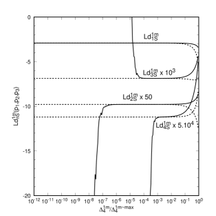
Figure 6: The finite functions for the box graph with two adjacent massive legs as a function of $\Delta_{4}^{1m}/\Delta_{4}^{1m~{}{\rm max}}$. The functions have been evaluated in double precision Fortran. The dashed lines show the approximate form for the function in the limit $\Delta_{4}^{1m}\to 0$, retaining only the first term of the Taylor expansion as given in Appendix C.

Unlike the $p_{1}^{2}\neq 0$ case, the scalar triangle pinchings all contain infrared poles and there is no benefit in absorbing the $m=3$ piece in the tensor integrals. Therefore we introduce,

$${\rm Ld}_{ni_{1}\ldots i_{n-1}}^{1m}(p_{1},p_{2},p_{3})=-n{\rm I}_{4}^{1m,D=6}[x_{i_{1}}\ldots x_{i_{n-1}}],$$ (4.22)

for $n=1,~{}2,~{}3$ and 4. Using equations (2.7–2.10) with $n=4$ and $D=4-2\epsilon$ we find,

$${\rm I}_{4}^{1m}[x_{i}] = \gamma_{i}{\rm Ld}_{1}^{1m}-\sum_{m=1}^{4}\eta_{im}\alpha_{i}\alpha_{m}{\rm I}_{3}^{(m)}[1],$$ (4.23)

$${\rm I}_{4}^{1m}[x_{i}x_{j}] = \gamma_{i}{\rm Ld}_{2j}^{1m}-\eta_{ij}\alpha_{i}\alpha_{j}{\rm Ld}_{1}^{1m}-\sum_{m=1}^{4}\eta_{im}\alpha_{i}\alpha_{m}{\rm I}_{3}^{(m)}[x_{j}],$$ (4.24)

$${\rm I}_{4}^{1m}[x_{i}x_{j}x_{k}] = \gamma_{i}{\rm Ld}_{3jk}^{1m}-\frac{1}{2}\eta_{ij}\alpha_{i}\alpha_{j}{\rm Ld}_{2k}^{1m}-\frac{1}{2}\eta_{ik}\alpha_{i}\alpha_{k}{\rm Ld}_{2j}^{1m}$$ (4.25)

$$\qquad-\sum_{m=1}^{4}\eta_{im}\alpha_{i}\alpha_{m}{\rm I}_{3}^{(m)}[x_{j}x_{k}],$$

$${\rm I}_{4}^{1m}[x_{i}x_{j}x_{k}x_{l}] = \gamma_{i}{\rm Ld}_{4jkl}^{1m}-\frac{1}{3}\eta_{ij}\alpha_{i}\alpha_{j}{\rm Ld}_{3kl}^{1m}-\frac{1}{3}\eta_{ik}\alpha_{i}\alpha_{k}{\rm Ld}_{3jl}^{1m}-\frac{1}{3}\eta_{il}\alpha_{i}\alpha_{l}{\rm Ld}_{3jk}^{1m}$$ (4.26)

$$\qquad-\sum_{m=1}^{4}\eta_{im}\alpha_{i}\alpha_{m}{\rm I}_{3}^{(m)}[x_{j}x_{k}x_{l}].$$

As in the previous section, the ${\rm Ld}_{ni_{1}\ldots i_{n-1}}^{1m}$ functions are finite as $\epsilon\to 0$ and contain no power-like divergences in the $s_{12}\to 0$, $s_{23}\to 0$ and $\Delta_{4}^{1m}\to 0$ limits. For convenience, explicit forms are given in Appendix B.

4.3 The opposite two-mass box

The two mass box graph where the massive legs sit on opposite sides is a special case because the scalar integral itself is not finite as $\Delta_{4}^{opp}\to 0$. We must therefore proceed with care. To make best use of the symmetry under $p_{1}\leftrightarrow p_{3}$, it is convenient to write,

$${\cal P}^{\mu}=-(1-x_{1})p_{1}^{\mu}-(x_{3}+x_{4})p_{2}^{\mu}-x_{4}p_{3}^{\mu}.$$

Under this flip symmetry, $x_{1}\leftrightarrow x_{4}$, $x_{2}\leftrightarrow x_{3}$ and

$${\cal P}^{\mu}\to-{\cal P}^{\mu}-p_{1}^{\mu}-p_{2}^{\mu}-p_{3}^{\mu}.$$

In this kinematic configuration, the $\alpha$ parameters can be defined by,

$$\begin{array}[]{rr}\alpha_{1}\alpha_{4}\,s_{123}=-\lambda,&\alpha_{2}\alpha_{3}\,p_{2}^{2}=-1\\ \alpha_{1}\alpha_{3}\,s_{12}=-1,&\alpha_{2}\alpha_{4}\,s_{23}=-1,\end{array}$$

where $\lambda$ is an extra kinematic variable that ensures that the $\alpha_{i}$ are independent,

$$\lambda=\frac{s_{123}p_{2}^{2}}{s_{12}s_{23}}.$$

With this choice of $\alpha_{i}$,

$$\eta_{ij}=(1-\lambda)\left(\begin{array}[]{rrrr}0&0&1&-1\\ 0&0&-\lambda&1\\ 1&-\lambda&0&0\\ -1&1&0&0\end{array}\right),\qquad N_{4}=\frac{1}{2}(1-\lambda)^{2}.$$

Each row of $\eta$ naturally couples together two of the pinchings (triangles) of this box, so we might expect such structure to dominate the integrals. The associated Gram determinant is given by,

$$\Delta_{4}^{opp}=2(s_{12}s_{23}-p_{2}^{2}s_{123})s_{13}=\frac{2(1-\lambda)s_{13}}{\prod_{i=1}^{4}\alpha_{i}},$$

where,

$$s_{13}=s_{123}-s_{12}-s_{23}+p_{2}^{2},$$

and,

$$\frac{\gamma_{i}}{\prod_{j=1}^{4}\alpha_{j}}=(1-\lambda)\left\{\begin{array}[]{ll}p_{2}^{2}-s_{23}&i=1\\ s_{123}-s_{12}&i=2\\ s_{123}-s_{23}&i=3\\ p_{2}^{2}-s_{12}&i=4\\ \end{array}\right..$$

We note that the presence of the Gram determinant is synonymous with a factor of $(1-\lambda)$.

The scalar integral for the opposite box in $D=4-2\epsilon$ is given by,

$$\hat{\rm I}_{4}^{opp}[1]=\frac{2}{(1-\lambda)}\left(\frac{c_{\Gamma}}{\epsilon^{2}}\left((\alpha_{1}\alpha_{3})^{\epsilon}+(\alpha_{2}\alpha_{4})^{\epsilon}-(\alpha_{2}\alpha_{3})^{\epsilon}-(\alpha_{1}\alpha_{4})^{\epsilon}\lambda^{-\epsilon}\right)+{\rm Ld}_{0}^{opp}(p_{1},p_{2},p_{3})\right)+{\cal O}(\epsilon),$$ (4.27)

where the finite part ${\rm Ld}_{0}$ can be written,

$${\rm Ld}_{0}^{opp}(p_{1},p_{2},p_{3}) = {\rm Li_{2}}\left(1-\lambda\right)+{\rm Li_{2}}\left(1-\frac{\alpha_{4}}{\lambda\alpha_{3}}\right)+{\rm Li_{2}}\left(1-\frac{\alpha_{1}}{\lambda\alpha_{2}}\right)$$ (4.28)

$$\quad-{\rm Li_{2}}\left(1-\frac{\alpha_{4}}{\alpha_{3}}\right)-{\rm Li_{2}}\left(1-\frac{\alpha_{1}}{\alpha_{2}}\right)+\log\left(\frac{\alpha_{4}}{\lambda\alpha_{3}}\right)\log\left(\frac{\alpha_{1}}{\lambda\alpha_{2}}\right).$$

As $\lambda\to 1$, there is a manifest singularity in $\hat{\rm I}_{4}^{opp}[1]$ since,

$${\rm Ld}_{0}^{opp}(p_{1},p_{2},p_{3})\to-\log\left(\frac{\alpha_{1}}{\alpha_{2}}\right)\log\left(\frac{\alpha_{3}}{\alpha_{4}}\right).$$

This double logarithm can never combine with lower point scalar integrals to form a combination well behaved as $\Delta_{4}^{opp}\to 0$. In fact, it is easy to see from fig. 4 that the only scalar integrals which are available by pinching are the triangle integrals with one and two massive legs. These are pure poles in $\epsilon$ and cannot be combined with the finite parts of the opposite box integral. There is no appropriate function which can generate the double logarithm as $\lambda\to 1$ and consequently no finite function can be formed. Since the matrix elements are in general finite in the limit of vanishing Gram determinants, all occurences of ${\rm Ld}_{0}^{opp}$ divided by the determinant must vanish.

On the other hand, in $D=6-2\epsilon$, the opposite box is not only finite as $\epsilon\to 0$ as expected, but also as $\lambda\to 1$. This is because $N_{4}$ is effectively $(\Delta^{opp}_{4})^{2}$ and its presence in the numerator of equation (2.4) removes the Gram determinant from the denominator. Consequently, we see that,

$${\rm I}_{4}^{opp~{}D=6-2\epsilon}[1]=-\frac{1}{s_{13}}{\rm Ld}_{0}^{opp}(p_{1},p_{2},p_{3}),$$ (4.29)

which, since,

$$\lim_{s_{13}\to 0}{\rm Ld}_{0}(p_{1},p_{2},p_{3}) = \frac{s_{13}}{s_{12}s_{23}-p_{2}^{2}s_{123}}\left(s_{12}\log\left(\frac{s_{123}}{s_{12}}\right)+s_{23}\log\left(\frac{s_{123}}{s_{23}}\right)-p_{2}^{2}\log\left(\frac{s_{123}}{p_{2}^{2}}\right)\right)$$ (4.30)

$$+{\cal O}(s_{13}^{2}),$$

is also finite as $s_{13}\to 0$.

In dealing with the all-massive triangle and adjacent box in the previous sections, we have constructed groups of scalar integrals that are finite both as $\epsilon\to 0$ and $\Delta\to 0$. For the opposite box, this is not easy to do since the raw scalar integral is not finite in either of these limits. Therefore, we follow the approach used for the two-mass triangle graph and obtain the tensor integrals by direct differentiation. However, we note that the factor $1/(n-D)$ associated with the differentiation formula (2.2) is itself divergent, implying that the ${\cal O}(\epsilon)$ term in $\hat{\rm I}_{4}^{opp}[1]$ is needed - the so called $\epsilon$-barrier. We circumvent this, by using equation (2.7), to construct the tensor integral with a single Feynman parameter. Explicitly, we find,

$$\hat{\rm I}_{4}^{opp}[a_{3}] = \frac{1}{(1-\lambda)}\Biggl{\{}\frac{(\alpha_{1}-\lambda\alpha_{2}){\rm Ld}_{0}^{opp}(p_{1},p_{2},p_{3})}{\alpha_{1}\alpha_{3}+\alpha_{2}\alpha_{4}-\alpha_{1}\alpha_{4}-\lambda\alpha_{2}\alpha_{3}}$$ (4.31)

$$\qquad-\frac{c_{\Gamma}}{\epsilon^{2}}\left(\frac{(\alpha_{2}\alpha_{4})^{\epsilon}-(\alpha_{2}\alpha_{3})^{\epsilon}}{\alpha_{4}-\alpha_{3}}\right)+\frac{\lambda c_{\Gamma}}{\epsilon^{2}}\left(\frac{(\alpha_{1}\alpha_{4})^{\epsilon}\lambda^{-\epsilon}-(\alpha_{1}\alpha_{3})^{\epsilon}}{\alpha_{4}-\lambda\alpha_{3}}\right)\Biggr{\}},$$

$$\hat{\rm I}_{4}^{opp}[a_{4}] = \frac{1}{(1-\lambda)}\Biggl{\{}\frac{(\alpha_{2}-\alpha_{1}){\rm Ld}_{0}^{opp}(p_{1},p_{2},p_{3})}{\alpha_{1}\alpha_{3}+\alpha_{2}\alpha_{4}-\alpha_{1}\alpha_{4}-\lambda\alpha_{2}\alpha_{3}}$$ (4.32)

$$\qquad+\frac{c_{\Gamma}}{\epsilon^{2}}\left(\frac{(\alpha_{2}\alpha_{4})^{\epsilon}-(\alpha_{2}\alpha_{3})^{\epsilon}}{\alpha_{4}-\alpha_{3}}\right)-\frac{c_{\Gamma}}{\epsilon^{2}}\left(\frac{(\alpha_{1}\alpha_{4})^{\epsilon}\lambda^{-\epsilon}-(\alpha_{1}\alpha_{3})^{\epsilon}}{\alpha_{4}-\lambda\alpha_{3}}\right)\Biggr{\}}.$$

This is enough to construct all the necessary integrals, since those for $a_{2}$ and $a_{1}$ can be obtained by the simultaneous exchanges, $a_{1}\leftrightarrow a_{4}$, $a_{2}\leftrightarrow a_{3}$ (and $p_{1}\leftrightarrow p_{3}$), while integrals with higher powers can be obtained by direct differentiation. The only subtlety is in differentiating ${\rm Ld}_{0}$, where it is useful to re-express some of the logarithms as single poles in $\epsilon$. For example,

$$\frac{\partial{\rm Ld}_{0}(p_{1},p_{2},p_{3})}{\partial\alpha_{4}}=\frac{\log\left(\frac{\alpha_{4}}{\alpha_{3}}\right)}{\alpha_{4}-\alpha_{3}}-\frac{\log\left(\frac{\alpha_{4}}{\lambda\alpha_{3}}\right)}{\alpha_{4}-\lambda\alpha_{3}}+\frac{c_{\Gamma}}{\epsilon}\left(\frac{(\alpha_{1}\alpha_{4})^{\epsilon}\lambda^{-\epsilon}-(\alpha_{2}\alpha_{4})^{\epsilon}}{\alpha_{4}}\right)+{\cal O}(\epsilon).$$

This helps to ensure that although the double poles in $\epsilon$ are still divided by $(1-\lambda)$, the single poles are finite as $\lambda\to 1$. In fact, when the tensor integral is multipled by a factor of $\epsilon$ we also expect that the resulting single logarithms occur in groups that are finite as $\lambda\to 1$. We therefore introduce the auxiliary functions,

$${\rm Lcd}_{n}(p_{1},p_{2},p_{3}) = -\lim_{\epsilon\to 0}\left(\epsilon\times{\rm I}_{4}^{opp}[x_{4}^{n}]\right)$$ (4.33)

$$= -\frac{1}{(1-\lambda)}\lim_{\epsilon\to 0}\left(\alpha_{4}\alpha_{1}{\rm I}_{3}^{(1)}[x_{4}^{n-1}]-\alpha_{4}\alpha_{2}{\rm I}_{3}^{(2)}[x_{4}^{n-1}]\right)$$

$$= \frac{2s_{13}}{\Delta_{4}^{opp}}\left(s_{12}{\rm Lc}_{n}^{2m}(p_{12},p_{3})-p_{2}^{2}{\rm Lc}_{n}^{2m}(p_{2},p_{3})\right),$$

for $n=1,\ldots,4$ and,

$${\rm Lcd}_{0}(p_{1},p_{2},p_{3})=\frac{2s_{13}}{\Delta_{4}^{opp}}\log\left(\frac{s_{12}s_{23}}{p_{2}^{2}s_{123}}\right).$$ (4.34)

Because these functions contain only a single power of the Gram determinant, they are not difficult to evaluate numerically.

The tensor integrals are straightforward to derive, but can be rather lengthy, for example,

$${\rm I}_{4}^{opp}[x_{4}^{2}] = -\frac{(\prod_{i}\alpha_{i})\alpha_{4}^{2}}{1-2\epsilon}\frac{\partial}{\partial\alpha_{4}}\hat{\rm I}^{opp}_{4}[a_{4}]$$ (4.35)

$$= \frac{c_{\Gamma}}{\epsilon^{2}}\frac{2s_{13}}{\Delta_{4}^{opp}}\Biggl{(}\frac{s_{12}^{2}\left((-s_{12})^{-\epsilon}-(-s_{123})^{-\epsilon}\right)}{(s_{123}-s_{12})^{2}}-\frac{p_{2}^{4}\left((-p_{2}^{2})^{-\epsilon}-(-s_{23})^{-\epsilon}\right)}{(s_{23}-p_{2}^{2})^{2}}\Biggr{)}$$

$$\qquad+\frac{c_{\Gamma}}{\epsilon}\frac{1}{s_{13}}\Biggl{(}\frac{(-s_{123})^{-\epsilon}}{(s_{123}-s_{12})}-\frac{(-s_{23})^{-\epsilon}}{(s_{23}-p_{2}^{2})}\Biggr{)}+\frac{2(s_{12}-p_{2}^{2})^{2}}{s_{13}\Delta_{4}^{opp}}{\rm Ld}_{0}(p_{1},p_{2},p_{3})$$

$$\qquad-\frac{(s_{12}-p_{2}^{2})}{s_{13}}{\rm Lcd}_{1}(p_{1},p_{2},p_{3})-2{\rm Lcd}_{2}(p_{1},p_{2},p_{3}).$$

Most of these terms are poles in $\epsilon$. For physical processes, the $1/\epsilon^{2}$ poles from different tensor integrals must combine in such a way that the $\Delta^{opp}_{4}$ cancels, while the $1/\epsilon$ poles do not depend on the determinant and are ready to cancel with contributions from other loop configurations. In all cases, the scalar box function ${\rm Ld}_{0}$ is associated with a single inverse power of $\Delta_{4}^{opp}$. As noted earlier, for physical processes that are finite as $\Delta_{4}^{opp}\to 0$, there must be cancellations amongst the various tensor integrals so that no terms containing ${\rm Ld}_{0}/\Delta_{4}^{opp}$ remain. We therefore choose to leave the ${\rm Ld}_{0}$ functions exposed to facilitate the cancellation of these terms.

For third and fourth rank tensor integrals, we also need to know the $D=6-2\epsilon$ box with one or two Feynman parameters in the numerator and the $D=8-2\epsilon$ box. The former are finite as $\epsilon\to 0$ and are easily obtained by direct differentiation of ${\rm I}_{4}^{opp~{}D=6-2\epsilon}[1]$ so that, for example,

$${\rm I}_{4}^{opp~{}D=6-2\epsilon}[x_{4}] = \frac{1}{2s_{13}}\Biggl{\{}\frac{(s_{12}-p_{2}^{2})}{s_{13}}{\rm Ld}_{0}(p_{1},p_{2},p_{3})-s_{12}{\rm Lc}_{1}^{2m}(p_{12},p_{3})$$ (4.36)

$$\qquad+p_{2}^{2}{\rm Lc}_{1}^{2m}(p_{2},p_{3})-\log\left(\frac{s_{123}}{s_{23}}\right)\Biggr{\}},$$

while the $D=8-2\epsilon$ box is established using the dimension changing equation (2.4),

$${\rm I}_{4}^{opp~{}D=8-2\epsilon}[1] = \frac{1}{6s_{13}}\Biggl{\{}\frac{s_{12}s_{23}-p_{2}^{2}s_{123}}{s_{13}}{\rm Ld}_{0}(p_{1},p_{2},p_{3})-s_{12}\log\left(\frac{s_{123}}{s_{12}}\right)-s_{23}\log\left(\frac{s_{123}}{s_{23}}\right)$$ (4.37)

$$\qquad+p_{2}^{2}\log\left(\frac{s_{123}}{p_{2}^{2}}\right)\Biggr{\}}+\frac{1}{6}\left(\frac{(-s_{123})^{-\epsilon}}{\epsilon}+\frac{11}{3}\right)c_{\Gamma}.$$

As might be expected, both of these are finite as $s_{13}\to 0$ and this can be seen directly from equation (4.30).

In summary, the situation for box integrals is very similar to that for triangle graphs. When the scalar integral is finite as $\Delta_{4}\to 0$, differentiating - or equivalently adding factors of Feynman parameters - does not introduce kinematic singularities. Hence natural groupings of box and triangle integrals arise that are finite as $\Delta_{4}\to 0$. Furthermore, the infrared and ultraviolet singularities can be isolated easily. Although we have explicitly worked through a subset of kinematic configurations relevant to certain QCD processes, this method is systematic and can be applied to processes with more general kinematics (and particularly non-zero internal masses).

5 Five point integrals

In this section we consider five point integrals with only one external mass. The outflowing lightlike momenta are denoted $p_{i}$, $i=1,\ldots,4$ while the fifth $p_{5}=-p_{1234}$ is massive, $p_{5}^{2}\neq 0$ as shown in fig. 7. The auxiliary momentum is then,

$${\cal P}^{\mu}=-(1-x_{1})p_{1}^{\mu}-(1-x_{1}-x_{2})p_{2}^{\mu}-(x_{4}+x_{5})p_{3}^{\mu}-x_{5}p_{4}^{\mu}.$$

We can make the choice,

$$\begin{array}[]{rr}\alpha_{1}\alpha_{5}\,s_{1234}=-\lambda,&\alpha_{2}\alpha_{4}\,s_{23}=-1\\ \alpha_{1}\alpha_{3}\,s_{12}=-1,&\alpha_{2}\alpha_{5}\,s_{234}=-1\\ \alpha_{1}\alpha_{4}\,s_{123}=-1,&\alpha_{3}\alpha_{5}\,s_{34}=-1,\end{array}$$

with,

$$(1-\lambda)=\frac{1}{\alpha_{3}}\prod_{i=1}^{5}\alpha_{i}(s_{123}s_{234}-s_{23}s_{1234}).$$

As in the opposite box integral, $\lambda$ is an extra kinematic variable that ensures the $\alpha_{i}$ are independent. It is the same variable that occurs in the third pinching which forms an opposite box configuration. The matrix $\eta_{ij}$ is given by,

$$\eta_{ij}=\left(\begin{array}[]{ccccc}1&-1&1-\lambda&1&-1\\ -1&1&\lambda-1&1-2\lambda&1\\ 1-\lambda&\lambda-1&(1-\lambda)^{2}&\lambda-1&1-\lambda\\ 1&1-2\lambda&\lambda-1&1&-1\\ -1&1&1-\lambda&-1&1\end{array}\right),$$

and the normalisation factor is,

$$N_{5}=1-\lambda.$$

The $\gamma_{i}$ are rather lengthy, but can be read off from $\eta_{ij}$.

Figure 7: The pentagon graph and each of the five pinchings obtained by omitting the internal line associated with $\alpha_{m}$ for $m=1,2,3,4$ and 5. For box pinchings, the entering momentum is fixed by momentum conservation.

The scalar pentagon integral is by now well-known in $D=4$ [20, 14, 3] and in $D=4-2\epsilon$ [4, 8, 9] and can be written in terms of these variables as,

$$\hat{\rm I}_{5}[1]=-\frac{1}{2N_{5}}\sum_{m=1}^{5}\hat{\gamma}_{m}\hat{\rm I}_{4}^{(m)}[1]+\cal{O}(\epsilon).$$ (5.1)

The five pinchings and the momenta associated with each is illustrated in fig. 7. The limit $N_{5}\rightarrow 0$ corresponds to the vanishing of the Gram determinant associated with the $m=3$ pinching. The scalar integral for this pinching is not well behaved in this limit and so should not be expected to combine with the other pinchings. Therefore, we separate $\hat{\rm I}_{5}[1]$ according to the pole structure in $\epsilon$ and $N_{5}$. We identify the function ${\rm Le}_{1}$ which is finite as both $N_{5}\rightarrow 0$ and $\epsilon\to 0$ and does not depend on the opposite-box pinching, $m=3$, plus a combination of scalar box integrals containing all the infrared poles and the remaining $N_{5}\to 0$ singularities,

$${\rm I}_{5}[1] = \left(\sum_{i=1}^{5}\alpha_{3}\alpha_{i}\kappa_{i}\right){\rm Le}_{1}-\frac{1}{2N_{5}}\gamma_{3}{\rm I}_{4}^{(3)}[1]-\alpha_{2}\alpha_{4}\left({\rm I}_{4}^{(2)}[1]+{\rm I}_{4}^{(4)}[1]\right)$$ (5.2)

$$-\frac{1}{2}\alpha_{3}\left(\alpha_{1}{\rm I}_{4}^{(1)}[1]-\alpha_{2}{\rm I}_{4}^{(2)}[1]-\alpha_{4}{\rm I}_{4}^{(4)}[1]+\alpha_{5}{\rm I}_{4}^{(5)}[1]\right),$$

where $\kappa_{i}=(1,-1,0,1,-1)$ and,

$${\rm Le}_{1}=-\frac{\alpha_{1}\alpha_{2}\alpha_{4}\alpha_{5}}{2N_{5}}\sum_{m=1}^{5}\kappa_{m}\hat{\rm I}_{4}^{(m)}[1].$$ (5.3)

Applying equation (2.7) and noting that ${\rm I}_{5}^{D=6}$ is both infrared and ultraviolet finite, the integrals with one insertion are also determined in terms of box integrals in $D=4-2\epsilon$ dimensions,

$$\hat{\rm I}_{5}[a_{i}]=-\frac{1}{2N_{5}}\sum_{m=1}^{5}\eta_{im}\hat{\rm I}_{4}^{(m)}[1]+\cal{O}(\epsilon).$$ (5.4)

Making the same separation as before,

$${\rm I}_{5}[x_{i}]=\left(\alpha_{3}\alpha_{i}\kappa_{i}\right){\rm Le}_{1}-\frac{1}{2N_{5}}\sum_{m=1}^{5}\alpha_{i}\alpha_{m}\left(\eta_{im}-\kappa_{i}\kappa_{m}\right){\rm I}_{4}^{(m)}[1]+\cal{O}(\epsilon),$$ (5.5)

where the bracket multiplying the scalar box integral is always proportional to $N_{5}$.

Similarly, using the usual formula for two Feynman parameters (2.8) and concentrating all of the $\Delta_{5}$ dependence into $\hat{c}_{i,j}$, where,

$$c_{i,j}=\alpha_{i}\alpha_{j}\hat{c}_{i,j}=\frac{\alpha_{i}\alpha_{j}}{2N_{5}}\left(\eta_{ij}-\frac{\hat{\gamma}_{i}\hat{\gamma}_{j}}{\hat{\Delta}_{5}}\right),$$ (5.6)

we find,

$$\hat{\rm I}_{5}[a_{i}a_{j}] = \hat{c}_{i,j}\left(\hat{\rm I}_{5}^{D=6}[1]+\frac{1}{2N_{5}}\sum_{m=1}^{5}\hat{\gamma}_{m}\hat{\rm I}_{4}^{D=6,(m)}[1]\right)$$ (5.7)

$$+\frac{1}{4N_{5}^{2}}\sum_{m=1}^{5}(\eta_{im}\hat{\gamma}_{j}-\eta_{ij}\hat{\gamma}_{m})\hat{\rm I}_{4}^{D=6,(m)}[1]-\frac{1}{2N_{5}}\sum_{m=1}^{5}\eta_{jm}\hat{\rm I}_{4}^{(m)}[a_{i}]$$

$$= -\hat{c}_{i,j}\frac{\hat{\Delta}_{5}\hat{\rm I}_{5}^{D=8}[1]}{N_{5}}$$

$$+\frac{1}{2N_{5}}\sum_{m=1}^{5}\left(\left(\frac{\hat{\gamma}^{(m)}_{j}\eta_{im}-\hat{\gamma}_{m}\eta_{ij}^{(m)}}{\eta_{mm}}\right)\hat{\rm I}_{4}^{D=6,(m)}[1]-\eta_{jm}\hat{\rm I}_{4}^{(m)}[a_{i}]\right).$$

To simplify the non-$\hat{c}_{i,j}$ terms (and eliminate one power of $N_{5}$), we have rewritten some of the variables appropriate to the pentagon integral in terms of those appropriate to the box pinchings, $\eta_{ij}^{(m)}$ and $\hat{\gamma}_{i}^{(m)}$, using the relations [9],

$$\gamma_{i}^{(m)}=\frac{\eta_{mm}\gamma_{i}-\eta_{im}\gamma_{m}}{2N_{5}},\qquad\eta_{ij}^{(m)}=\frac{\eta_{mm}\eta_{ij}-\eta_{im}\eta_{jm}}{2N_{5}}.$$

Bern, Dixon and Kosower have shown [8, 9] that ${\rm I}_{5}^{6}$ drops out of the calculation of any gauge theory amplitudes by using the identity [4],

$$\sum_{i,j=1}^{4}q_{i}^{\mu_{i}}q_{j}^{\mu_{j}}c_{i+1,j+1}=\frac{1}{2}g^{\mu_{i}\mu_{j}}_{[4]},$$ (5.8)

where $g^{\mu_{i}\mu_{j}}_{[4]}$ represents the metric tensor in $D=4$. Since,

$${\rm I}_{5}[\ell^{\mu_{i}}\ell^{\mu_{j}}] = {\rm I}_{5}[{\cal P}^{\mu_{i}}{\cal P}^{\mu_{j}}]-\frac{1}{2}{\rm I}_{5}^{D=6}[1]g^{\mu_{i}\mu_{j}}$$ (5.9)

$$= \sum_{i,j=1}^{5}{\rm I}_{5}[x_{i+1}x_{j+1}]q_{i}^{\mu_{i}}q_{j}^{\mu_{j}}-\frac{1}{2}{\rm I}_{5}^{D=6}[g^{\mu_{i}\mu_{j}}],$$

all terms proportional to $\hat{c}_{i,j}$ in $\hat{\rm I}_{5}[a_{i}a_{j}]$ can be moved into the existing $g^{\mu_{i}\mu_{j}}$ piece. Inspection of equation (5.7) indicates that the correct term to reshuffle is $-\Delta_{5}\hat{\rm I}_{5}^{8}[1]/N_{5}$ rather than merely $\hat{\rm I}_{5}^{D=6}[1]$. Retaining only the $c_{i,j}$ terms,

$$g^{\mu_{i}\mu_{j}}\mbox{ terms} = -\frac{1}{2}{\rm I}_{5}^{D=6}[1]g^{\mu_{i}\mu_{j}}-\frac{\hat{\Delta}_{5}{\rm I}_{5}^{D=8}[1]}{N_{5}}\sum_{i,j=1}^{4}q_{i}^{\mu_{i}}q_{j}^{\mu_{j}}c_{i+1,j+1}$$ (5.10)

$$= -\frac{1}{2}{\rm I}_{5}^{D=6}[1]g^{\mu_{i}\mu_{j}}+\frac{1}{2}\left({\rm I}_{5}^{D=6}[1]+\frac{1}{2N_{5}}\sum_{m=1}^{5}\gamma_{m}{\rm I}_{4}^{D=6,(m)}[1]\right)g^{\mu_{i}\mu_{j}}_{[4]}$$

$$= \frac{1}{4N_{5}}\sum_{m=1}^{5}\gamma_{m}{\rm I}_{4}^{D=6,(m)}[1]g^{\mu_{i}\mu_{j}}+{\cal O}(\epsilon).$$

As expected the ${\rm I}_{5}^{D=6}[1]$ terms precisely cancel. Here the finiteness of ${\rm I}_{5}^{D=6}[1]$ and ${\rm I}_{5}^{D=8}[1]$ has been used to ensure that this term generates only ${\cal O}(\epsilon)$ corrections when replacing $g^{\mu_{i}\mu_{j}}_{[4]}$ with the dimensionally regularised $g^{\mu_{i}\mu_{j}}$. The remaining piece should not contain any kinematic singularities associated with lower-point Gram determinants, in particular $N_{5}$, as it originates from the well-behaved ${\rm I}_{5}^{D=8}$. This is indeed the case and we write,

$${\rm Le}_{2}=\frac{1}{2N_{5}}\sum_{m=1}^{5}\gamma_{m}{\rm I}_{4}^{D=6,(m)}[1].$$ (5.11)

The pentagon integrals with three insertions can be obtained by direct differentiation of equation (5.7). We find,

$$\hat{\rm I}_{5}[a_{i}a_{j}a_{k}] = \hat{c}_{i,j}\left(\hat{\rm I}_{5}^{D=6}[a_{k}]+\frac{1}{6N_{5}}\sum_{m=1}^{5}\left(\eta_{km}\hat{\rm I}_{4}^{D=6,(m)}[1]+2\hat{\gamma}_{m}\hat{\rm I}_{4}^{D=6,(m)}[a_{k}]\right)\right)$$ (5.12)

$$+\frac{1}{6N_{5}}\sum_{m=1}^{5}\Biggl{(}2\left(\frac{\hat{\gamma}^{(m)}_{j}\eta_{im}-\hat{\gamma}_{m}\eta_{ij}^{(m)}}{\eta_{mm}}\right)\hat{\rm I}_{4}^{D=6,(m)}[a_{k}]$$

$$-\left(\frac{\eta_{im}\eta_{jk}^{(m)}-\eta_{ij}^{(m)}\eta_{km}}{\eta_{mm}}\right)\hat{\rm I}_{4}^{D=6,(m)}[1]-\eta_{jm}\hat{\rm I}_{4}^{(m)}[a_{i}a_{k}]\Biggr{)}+\mbox{cyclic i,j,k}.$$

Since the $\hat{c}_{i,j}$ term is obtained by differentiating $c_{i,j}{\rm I}_{5}^{D=8}[1]$, it must be finite as both $N_{5}\to 0$ and $\epsilon\to 0$ and we introduce the finite function,

$${\rm Le}_{3k}=\frac{1}{6N_{5}}\sum_{m=1}^{5}\left(\alpha_{k}\alpha_{m}\eta_{km}{\rm I}_{4}^{D=6,(m)}[1]+2\gamma_{m}{\rm I}_{4}^{D=6,(m)}[x_{k}]\right).$$ (5.13)

Recalling that,

$${\rm I}_{5}[\ell^{\mu_{i}}\ell^{\mu_{j}}\ell^{\mu_{k}}] = {\rm I}_{5}[{\cal P}^{\mu_{i}}{\cal P}^{\mu_{j}}{\cal P}^{\mu_{k}}]-\frac{1}{2}{\rm I}_{5}^{D=6}[\{g{\cal P}\}^{\mu_{i}\mu_{j}\mu_{k}}]$$ (5.14)

$$= -\sum_{i,j,k=1}^{5}{\rm I}_{5}[x_{i+1}x_{j+1}x_{k+1}]q_{i}^{\mu_{i}}q_{j}^{\mu_{j}}q_{k}^{\mu_{k}}$$

$$+\frac{1}{2}\left\{\sum_{k=1}^{5}{\rm I}_{5}^{D=6}[x_{k+1}]g^{\mu_{i}\mu_{j}}q_{k}^{\mu_{k}}+\mbox{cyclic i,j,k}\right\},$$

and keeping only the $c_{i,j}$ terms in equation (5.12) we find,

$$g^{\mu_{i}\mu_{j}}q_{k}^{\mu_{k}}\mbox{ terms} = \frac{1}{2}{\rm I}_{5}^{D=6}[x_{k+1}]g^{\mu_{i}\mu_{j}}q_{k}^{\mu_{k}}-\left({\rm I}_{5}^{D=6}[x_{k+1}]+{\rm Le}_{3k}\right)\sum_{i,j=1}^{4}c_{i+1,j+1}q_{i}^{\mu_{i}}q_{j}^{\mu_{j}}q_{k}^{\mu_{k}}$$ (5.15)

$$= \frac{1}{2}{\rm I}_{5}^{D=6}[x_{k+1}]g^{\mu_{i}\mu_{j}}q_{k}^{\mu_{k}}-\frac{1}{2}\left({\rm I}_{5}^{D=6}[x_{k+1}]+{\rm Le}_{3k}\right)g^{\mu_{i}\mu_{j}}_{[4]}q_{k}^{\mu_{k}}$$

$$= -\frac{1}{2}{\rm Le}_{3k}g^{\mu_{i}\mu_{j}}q_{k}^{\mu_{k}}+{\cal O}(\epsilon).$$

As in the previous case, the finiteness of the coefficient of $g^{\mu_{i}\mu_{j}}_{[4]}$ has been used to promote it to the full $D=4-2\epsilon$ metric tensor.

The tensor integrals with four and five insertions may be obtained by further differentiation, and the same trick used to rewrite the $c_{i,j}$ terms as a contribution to the metric tensor structure. In this way, all vestiges of the pentagon in $D=6-2\epsilon$ and higher dimensions can be removed, along with the inverse powers of $\Delta_{5}$.

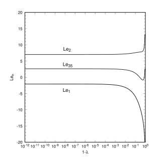
Figure 8: The finite functions for the pentagon graph with one external mass and evaluated in double precision Fortran as a function of $1-\lambda$. Because the functions only contain single inverse powers of $(1-\lambda)$, no numerical problems are evident.

The functions introduced in this section, ${\rm Le}_{1}$, ${\rm Le}_{2}$ and ${\rm Le}_{3i}$, only contain a single power of the Gram determinant. Consequently, they can be evaluated without numerical problems. To illustrate this, we choose a representative phase space point, $s_{1234}=1,~{}s_{123}=0.4,~{}s_{234}=0.3,~{}s_{13}=0.1$ and use the variable $s_{23}$ to control $\lambda$. The sixth variable $s_{24}$ is chosen to lie within the physical region defined by the pentagon Gram determinant, $\Delta_{5}<0$. Fig. 8 shows the functions ${\rm Le}_{1}$ and ${\rm Le}_{2}$ together with ${\rm Le}_{35}$. In each case, we see that the $\lambda\to 1$ limit is smoothly approached indicating that the function is intrinsically well behaved in that limit.

6 Conclusions

In this paper we have developed a new strategy for evaluating one-loop tensor integrals. It avoids the usual problems associated with the presence of Gram determinants. Such Gram determinants arise when the tensor integrals are expressed in terms of the physical momenta and generate false singularities at the edges of phase space. In addition to creating numerical instabilities, they tend to increase the size of the one-loop matrix elements. Our approach is to construct groups of scalar integrals which are well behaved in the limit of vanishing Gram determinant ($\Delta_{n}\to 0$), and which can be evaluated with arbitrary precision by making a Taylor series expansion in $\Delta_{n}$. In fact such combinations arise naturally by either differentiating with respect to the external parameters - essentially yielding scalar integrals with Feynman parameters in the numerator - or by developing the scalar integral in $D=6-2\epsilon$ or higher dimensions. Evaluating these new integrals is straightforward - they are just linear combinations of the known scalar integrals in $D=4$ or $D=4-2\epsilon$. As such, they combine the dilogarithms, logarithms and constants from different scalar integrals in an extremely non-trivial way. As a bonus other spurious kinematic singularities are also controlled - they appear in the denominator of the finite functions, which are well behaved in the singular limit. Although the number of basic functions has increased, the number of dilogarithm evaluations has not, since the functions are generated recursively. Furthermore, because the Gram determinant singularities are not genuine, by grouping integrals in this way, the expressions for one loop integrals are compactified.

To illustrate the approach for specific integrals, we have applied the method to 3-, 4- and 5-point integrals where the internal masses have been set equal to zero. These tensor integrals are relevant for a range of QCD processes where the quark and gluon masses are negligible. For more general processes with arbitrary internal masses and external kinematics, the relevant combinations of scalar integrals can be obtained using equations (2.4,2.7–2.10). As a by-product we have shown how all the Gram determinants associated with pentagon graphs can be eliminated.

Appendix A Triangle integrals

In this appendix, we collect together explicit forms for the triangle graphs which appear as building blocks in the box graphs. We fix the kinematics according to fig. 1, so that momenta $p_{1}$ and $p_{2}$ are exiting, with $p_{3}$ determined by momentum conservation. There are two distinct cases, according to whether one or two of the external masses are zero.

A.1 The one-mass triangle

Here we provide explicit results for the case $p_{1}^{2}=p_{2}^{2}=0$. There is an additional symmetry under the exchange $p_{1}\leftrightarrow p_{2}$ and $x_{1}\leftrightarrow x_{3}$. Insertions involving $x_{2}$ can be eliminated using $x_{1}+x_{2}+x_{3}=1$.

The $D=4-2\epsilon$ scalar and tensor integrals are given by,

$${\rm I}^{1m}_{3}[1] = \frac{c_{\Gamma}}{\epsilon^{2}}\frac{(-s_{12})^{-\epsilon}}{s_{12}},$$ (A.1)

$${\rm I}^{1m}_{3}[x_{1}]={\rm I}^{1m}_{3}[x_{3}]=2{\rm I}^{1m}_{3}[x_{1}^{2}]=2{\rm I}^{1m}_{3}[x_{3}^{2}] = -\frac{1}{s_{12}}\left(\frac{(-s_{12})^{-\epsilon}}{\epsilon}+2\right)c_{\Gamma},$$ (A.2)

$${\rm I}^{1m}_{3}[x_{1}x_{3}]=3{\rm I}^{1m}_{3}[x_{1}^{2}x_{3}]=3{\rm I}^{1m}_{3}[x_{1}x_{3}^{2}] = \frac{1}{2s_{12}},$$ (A.3)

$${\rm I}^{1m}_{3}[x_{1}^{3}]={\rm I}^{1m}_{3}[x_{3}^{3}] = -\frac{1}{3s_{12}}\left(\frac{(-s_{12})^{-\epsilon}}{\epsilon}+\frac{13}{6}\right)c_{\Gamma},$$ (A.4)

while, the necessary integrals in $D=6-2\epsilon$ dimensions read,

$${\rm I}^{1m,D=6-2\epsilon}_{3}[1] = -\frac{1}{2}\left(\frac{(-s_{12})^{-\epsilon}}{\epsilon}+3\right)c_{\Gamma},$$ (A.5)

$${\rm I}^{1m,D=6-2\epsilon}_{3}[x_{1}]={\rm I}^{1m,D=6-2\epsilon}_{3}[x_{3}] = -\frac{1}{6}\left(\frac{(-s_{12})^{-\epsilon}}{\epsilon}+\frac{8}{3}\right)c_{\Gamma}.$$ (A.6)

A.2 The two-mass triangle

When two of the external legs are massive, $p_{2}^{2}=0$ but $s_{12},~{}p_{1}^{2}\neq 0$, the divergent integrals read,

$${\rm I}^{2m}_{3}[1] = \frac{c_{\Gamma}}{\epsilon^{2}}\left(\frac{(-s_{12})^{-\epsilon}-(-p_{1}^{2})^{-\epsilon}}{s_{12}-p_{1}^{2}}\right),$$ (A.7)

$${\rm I}^{2m}_{3}[x_{3}] = -2{\rm Lc}_{2}^{2m}(p_{1},p_{2})-\frac{c_{\Gamma}}{\epsilon}\frac{(-s_{12})^{-\epsilon}}{(s_{12}-p_{1}^{2})}-\frac{p_{1}^{2}}{(s_{12}-p_{1}^{2})}{\rm I}^{2m}_{3}[1],$$ (A.8)

$${\rm I}^{2m}_{3}[x_{3}^{2}] = -3{\rm Lc}_{3}^{2m}(p_{1},p_{2})+\frac{1}{2(s_{12}-p_{1}^{2})}-c_{\Gamma}\frac{(-s_{12})^{-\epsilon}}{\epsilon}\frac{(s_{12}-3p_{1}^{2})}{2(s_{12}-p_{1}^{2})^{2}}$$ (A.9)

$$\qquad+\frac{p_{1}^{4}}{(s_{12}-p_{1}^{2})^{2}}{\rm I}^{2m}_{3}[1],$$

$${\rm I}^{2m}_{3}[x_{3}^{3}] = -\frac{11}{3}{\rm Lc}_{4}^{2m}(p_{1},p_{2})+\frac{(s_{12}-2p_{1}^{2})}{2(s_{12}-p_{1}^{2})^{2}}-\frac{p_{1}^{6}}{(s_{12}-p_{1}^{2})^{3}}{\rm I}^{2m}_{3}[1]$$ (A.10)

$$\qquad-\frac{(-s_{12})^{-\epsilon}}{\epsilon}\left(\frac{1}{3(s_{12}-p_{1}^{2})}-\frac{p_{1}^{2}}{2(s_{12}-p_{1}^{2})^{2}}+\frac{p_{1}^{4}}{(s_{12}-p_{1}^{2})^{3}}\right)c_{\Gamma},$$

while,

$${\rm I}^{2m}_{3}[x_{1}]=2{\rm I}^{2m}_{3}[x_{1}^{2}]=3{\rm I}^{2m}_{3}[x_{1}^{3}] = {\rm Lc}_{1}^{2m}(p_{1},p_{2}),$$ (A.11)

$${\rm I}^{2m}_{3}[x_{1}x_{3}]=3{\rm I}^{2m}_{3}[x_{1}^{2}x_{3}] = \frac{1}{2}{\rm Lc}_{2}^{2m}(p_{1},p_{2}),$$ (A.12)

$${\rm I}^{2m}_{3}[x_{1}x_{3}^{2}] = \frac{1}{3}{\rm Lc}_{3}^{2m}(p_{1},p_{2}).$$ (A.13)

The functions ${\rm Lc}_{n}^{2m}(p_{1},p_{2})$ are defined by equations (3.19,3.20).

The $D=6-2\epsilon$ dimension integrals read,

$${\rm I}^{2m,D=6-2\epsilon}_{3}[1] = \frac{1}{2}\left(p_{1}^{2}{\rm Lc}_{1}^{2m}(p_{1},p_{2})-\left(\frac{(-s_{12})^{-\epsilon}}{\epsilon}+3\right)c_{\Gamma}\right),$$ (A.14)

$${\rm I}^{2m,D=6-2\epsilon}_{3}[x_{1}] = \frac{1}{6}\left(p_{1}^{2}{\rm Lc}_{1}^{2m}(p_{1},p_{2})-\left(\frac{(-s_{12})^{-\epsilon}}{\epsilon}+\frac{8}{3}\right)c_{\Gamma}\right),$$ (A.15)

$${\rm I}^{2m,D=6-2\epsilon}_{3}[x_{3}] = \frac{1}{6}\left(p_{1}^{2}{\rm Lc}_{2}^{2m}(p_{1},p_{2})-\left(\frac{(-s_{12})^{-\epsilon}}{\epsilon}+\frac{8}{3}\right)c_{\Gamma}\right).$$ (A.16)

The corresponding integrals for the case $p_{1}^{2}=0$, $p_{2}^{2}\neq 0$ can be obtained by using the above formulae with the substitutions,

$$p_{1}\leftrightarrow p_{2},\qquad x_{1}\leftrightarrow x_{3}.$$ (A.17)

The limit $p_{1}^{2}\to 0$ may also be safely taken. For example, using the fact that in this limit ${\rm Lc}_{n}^{2m}(p_{1},p_{2})\to 1/(n-1)/s_{12}$ and observing that all of the triangle loop integral contributions proportional to $1/\epsilon^{2}$ trivially drop out in eqs. (A.8)-(A.10), we see that,

$${\rm I}_{3}^{2m}[x_{3}^{n}]\to{\rm I}_{3}^{1m}[x_{3}^{n}].$$

Appendix B Box integrals

Here we collect together explicit forms for the some of the finite functions appearing in the box integrals. We fix the kinematics according to fig. 2, so that momenta $p_{1}$, $p_{2}$ and $p_{3}$ are exiting, with $p_{4}$ determined by momentum conservation.

B.1 The adjacent two-mass box

We first focus on the case where two of the adjacent external legs are massive, $p_{4}^{2}\neq 0$ and $p_{1}^{2}\neq 0$.

For integrals with a single Feynman parameter in the numerator, we have,

$${\rm Ld}_{1}(p_{1},p_{2},p_{3})=-\left({\rm Ld}_{1S}(p_{1},p_{2},p_{3})+{\rm Lc}_{0}(p_{1},p_{23})\right),$$ (B.1)

where the box function in $D=6$, ${\rm Ld}_{1S}$ is given by equation (4.3). When there are two Feynman parameters in the numerator, we eliminate $x_{3}$ using $x_{1}+x_{2}+x_{3}+x_{4}=1$ so there are only three relevant functions. Explicitly, we find,

$${\rm Ld}_{21}(p_{1},p_{2},p_{3}) = -\frac{2}{s_{12}}\left(3{\rm Ld}_{2S}(p_{1},p_{2},p_{3})+{\rm Lc}_{1S}(p_{1},p_{23})\right)-{\rm Lc}_{1}(p_{23},p_{1}),$$ (B.2)

$${\rm Ld}_{22}(p_{1},p_{2},p_{3}) = \frac{2(s_{123}-s_{12})}{s_{12}s_{23}}\left(3{\rm Ld}_{2S}(p_{1},p_{2},p_{3})+{\rm Lc}_{1S}(p_{1},p_{23})\right)$$ (B.3)

$$\qquad-\frac{s_{12}}{s_{23}}{\rm Lc}_{1}^{2m}(p_{1},p_{2})+\frac{s_{123}}{s_{23}}{\rm Lc}_{1}(p_{23},p_{1}),$$

$${\rm Ld}_{24}(p_{1},p_{2},p_{3}) = \frac{2(p_{1}^{2}-s_{12})}{s_{12}s_{23}}\left(3{\rm Ld}_{2S}(p_{1},p_{2},p_{3})+{\rm Lc}_{1S}(p_{1},p_{23})\right)$$ (B.4)

$$\qquad-\frac{s_{12}}{s_{23}}{\rm Lc}_{1}^{2m}(p_{12},p_{3})+\frac{p_{1}^{2}}{s_{23}}{\rm Lc}_{1}(p_{23},p_{1}).$$

The all massive triangle integral function in $D=6-2\epsilon$, ${\rm Lc}_{1S}$ is given by equation (3.11), the box integral function in $D=8-2\epsilon$ is given in equation (4.7) while the remaining triangle functions are given in Appendix A and equations (3.4–3.9). The functions for adjacent box integrals with three insertions of Feynman parameters contain the box in $D=10-2\epsilon$ (4.8) and triangle in $D=8-2\epsilon$ (3.14). All integrals can be obtained in terms of the following four functions,

$${\rm Ld}_{311}(p_{1},p_{2},p_{3}) = -\Biggl{(}\frac{12}{s_{12}^{2}}\left(5{\rm Ld}_{3S}(p_{1},p_{2},p_{3})+{\rm Lc}_{2S}(p_{1},p_{23})\right)$$ (B.5)

$$+\frac{(s_{12}+p_{1}^{2})}{s_{12}}{\rm Lc}_{3}(p_{23},p_{1})+\frac{s_{23}}{s_{12}}{\rm Lc}_{2}(p_{1},p_{23})\Biggr{)},$$

$${\rm Ld}_{314}(p_{1},p_{2},p_{3}) = \frac{12(p_{1}^{2}-s_{12})}{s_{12}^{2}s_{23}}\left(5{\rm Ld}_{3S}(p_{1},p_{2},p_{3})+{\rm Lc}_{2S}(p_{1},p_{23})\right)$$ (B.6)

$$+\frac{p_{1}^{4}}{s_{12}s_{23}}{\rm Lc}_{3}(p_{23},p_{1})-\frac{(s_{12}-p_{1}^{2})}{s_{12}}{\rm Lc}_{2}(p_{1},p_{23})$$

$$-\frac{s_{12}}{2s_{23}}{\rm Lc}_{1}^{2m}(p_{12},p_{3}),$$

$${\rm Ld}_{322}(p_{1},p_{2},p_{3}) = -\Biggl{(}\frac{12(s_{123}-s_{12})^{2}}{s_{12}^{2}s_{23}^{2}}\left(5{\rm Ld}_{3S}(p_{1},p_{2},p_{3})+{\rm Lc}_{2S}(p_{1},p_{23})\right)$$ (B.7)

$$+\frac{s_{123}(s_{12}s_{123}+p_{1}^{2}s_{123}-2p_{1}^{2}s_{12})}{s_{12}s_{23}^{2}}{\rm Lc}_{3}(p_{23},p_{1})-\frac{s_{12}}{2s_{23}}{\rm Lc}_{2}^{2m}(p_{1},p_{2})$$

$$+\frac{s_{12}(s_{12}-s_{123})}{2s_{23}^{2}}{\rm Lc}_{1}^{2m}(p_{12},p_{3})+\frac{s_{123}(s_{123}-2s_{12})}{s_{12}s_{23}}{\rm Lc}_{2}(p_{1},p_{23})$$

$$+\frac{(p_{1}^{2}s_{12}+s_{12}s_{23}-s_{12}s_{123})}{2s_{23}^{2}}{\rm Lc}_{1}^{2m}(p_{1},p_{2})\Biggr{)},$$

$${\rm Ld}_{344}(p_{1},p_{2},p_{3}) = -\Biggl{(}\frac{12(s_{12}-p_{1}^{2})^{2}}{s_{12}^{2}s_{23}^{2}}\left(5{\rm Ld}_{3S}(p_{1},p_{2},p_{3})+{\rm Lc}_{2S}(p_{1},p_{23})\right)$$ (B.8)

$$+\frac{p_{1}^{2}(p_{1}^{2}-2s_{12})}{s_{12}s_{23}}{\rm Lc}_{2}(p_{1},p_{23})+\frac{p_{1}^{4}(p_{1}^{2}-s_{12})}{s_{12}s_{23}^{2}}{\rm Lc}_{3}(p_{23},p_{1})$$

$$+\frac{s_{12}(s_{12}-p_{1}^{2})}{2s_{23}^{2}}{\rm Lc}_{1}^{2m}(p_{12},p_{3})+\frac{s_{12}}{2s_{23}}{\rm Lc}_{2}^{2m}(p_{12},p_{3})\Biggr{)}.$$

B.2 The one-mass box

For this kinematic configuration, only $p_{4}^{2}\neq 0$ and there is a ‘flip’ symmetry, so that functions related to the parameter $x_{4}$ are obtained from those related to $x_{1}$, by $p_{1}\longleftrightarrow p_{3}$. The box integrals in higher dimension are given by equations (4.18–4.21), and,

$${\rm Ld}_{1}^{1m}(p_{1},p_{2},p_{3})=-{\rm Ld}_{1S}^{1m}(p_{1},p_{2},p_{3}).$$ (B.9)

For two and three insertions, we find,

$${\rm Ld}_{21}^{1m}(p_{1},p_{2},p_{3}) = -\frac{1}{s_{12}}\left(6{\rm Ld}_{2S}^{1m}(p_{1},p_{2},p_{3})+s_{23}{\rm Lc}_{1}^{2m}(p_{23},p_{1})\right),$$ (B.10)

$${\rm Ld}_{22}^{1m}(p_{1},p_{2},p_{3}) = {\rm Ld}_{1}^{1m}(p_{1},p_{2},p_{3})-{\rm Ld}_{21}^{1m}(p_{1},p_{2},p_{3}),$$ (B.11)

and,

$${\rm Ld}_{311}^{1m}(p_{1},p_{2},p_{3}) = -\frac{1}{s_{12}^{2}}\Biggl{(}60{\rm Ld}_{3S}^{1m}(p_{1},p_{2},p_{3})+\frac{1}{2}s_{23}^{2}{\rm Lc}_{1}^{2m}(p_{23},p_{1})$$ (B.12)

$$+\frac{1}{2}s_{12}s_{23}{\rm Lc}_{2}^{2m}(p_{23},p_{1})\Biggr{)},$$

$${\rm Ld}_{314}^{1m}(p_{1},p_{2},p_{3}) = -\frac{1}{s_{12}s_{23}}\Biggl{(}60{\rm Ld}_{3S}^{1m}(p_{1},p_{2},p_{3})+\frac{1}{2}s_{23}^{2}{\rm Lc}_{1}^{2m}(p_{23},p_{1})$$ (B.13)

$$+\frac{1}{2}s_{12}^{2}{\rm Lc}_{1}^{2m}(p_{12},p_{3})\Biggr{)},$$

$${\rm Ld}_{322}^{1m}(p_{1},p_{2},p_{3}) = {\rm Ld}_{311}^{1m}(p_{1},p_{2},p_{3})+{\rm Ld}_{1}^{1m}(p_{1},p_{2},p_{3})-2{\rm Ld}_{21}^{1m}(p_{1},p_{2},p_{3}).$$ (B.14)

Appendix C Limits

In this section, we collect together suitable expansions of the various functions presented in this paper in the limit $\Delta_{n}\to 0$. These expressions represent the leading term in the expansion of the functions as a Taylor series in $\Delta_{n}$ and should be evaluated for $\Delta_{n}<\delta$, where $\delta$ can be determined numerically. Typically, $\delta\sim 10^{-4}\Delta_{n}^{{\rm max}}$ where $\Delta_{n}^{{\rm max}}$ is the largest value the Gram determinant can achieve. In general, for a given numerical precision, $acc$ the numerical problems occur when $\Delta\sim(acc)^{1/N}$ where $N$ is the number of Gram determinants in the denominator of the function.

C.1 The three-mass triangle

In the limit that $\Delta_{3}\to 0$, we have,

$${\rm Lc}_{0}(p_{1},p_{2}) \to \frac{1}{2p_{1}^{2}p_{2}^{2}s_{12}}\left(p_{1}^{2}(s_{12}+p_{2}^{2}-p_{1}^{2})\log\left(\frac{s_{12}}{p_{1}^{2}}\right)+p_{2}^{2}(s_{12}+p_{1}^{2}-p_{2}^{2})\log\left(\frac{s_{12}}{p_{2}^{2}}\right)\right),$$

$${\rm Lc}_{1S}(p_{1},p_{2}) \to \frac{1}{12p_{1}^{2}p_{2}^{2}s_{12}}\Biggl{(}p_{1}^{4}(s_{12}+p_{2}^{2}-p_{1}^{2})\log\left(\frac{s_{12}}{p_{1}^{2}}\right)+p_{2}^{4}(s_{12}+p_{1}^{2}-p_{2}^{2})\log\left(\frac{s_{12}}{p_{2}^{2}}\right)$$ (C.2)

$$\qquad+2p_{1}^{2}p_{2}^{2}s_{12}\Biggr{)},$$

$${\rm Lc}_{2S}(p_{1},p_{2}) \to \frac{1}{120p_{1}^{2}p_{2}^{2}s_{12}}\Biggl{(}p_{1}^{6}(s_{12}+p_{2}^{2}-p_{1}^{2})\log\left(\frac{s_{12}}{p_{1}^{2}}\right)+p_{2}^{6}(s_{12}+p_{1}^{2}-p_{2}^{2})\log\left(\frac{s_{12}}{p_{2}^{2}}\right)$$ (C.3)

$$\qquad+\frac{p_{1}^{2}p_{2}^{2}s_{12}}{2}(s_{12}+p_{1}^{2}+p_{2}^{2})\Biggr{)},$$

$${\rm Lc}_{3S}(p_{1},p_{2}) \to \frac{1}{1680p_{1}^{2}p_{2}^{2}s_{12}}\Biggl{(}p_{1}^{8}(s_{12}+p_{2}^{2}-p_{1}^{2})\log\left(\frac{s_{12}}{p_{1}^{2}}\right)+p_{2}^{8}(s_{12}+p_{1}^{2}-p_{2}^{2})\log\left(\frac{s_{12}}{p_{2}^{2}}\right)$$ (C.4)

$$\qquad+\frac{2p_{1}^{2}p_{2}^{2}s_{12}}{9}(s_{12}^{2}+p_{1}^{4}+p_{2}^{4}+s_{12}p_{1}^{2}+s_{12}p_{2}^{2}+p_{1}^{2}p_{2}^{2})\Biggr{)},$$

$${\rm Lc}_{1}(p_{1},p_{2}) \to \frac{1}{3p_{1}^{2}(s_{12}+p_{2}^{2}-p_{1}^{2})}\left((s_{12}-p_{2}^{2})\log\left(\frac{s_{12}}{p_{2}^{2}}\right)+2p_{1}^{2}-p_{1}^{4}{\rm Lc}_{0}(p_{1},p_{2})\right),$$ (C.5)

$${\rm Lc}_{2}(p_{1},p_{2}) \to \frac{1}{6p_{2}^{2}(s_{12}+p_{1}^{2}-p_{2}^{2})}\Biggl{(}-4p_{2}^{2}(s_{12}+p_{1}^{2}-p_{2}^{2}){\rm Lc}_{3}(p_{1},p_{2})$$ (C.6)

$$\qquad+s_{12}-p_{2}^{2}+3p_{1}^{2}p_{2}^{2}{\rm Lc}_{1}(p_{1},p_{2})-p_{1}^{4}{\rm Lc}_{1}(p_{2},p_{1})+p_{2}^{2}\log\left(\frac{s_{12}}{p_{2}^{2}}\right)\Biggr{)},$$

$${\rm Lc}_{3}(p_{1},p_{2}) \to \frac{1}{5p_{1}^{2}(s_{12}+p_{2}^{2}-p_{1}^{2})}\left((s_{12}-p_{2}^{2})\log\left(\frac{s_{12}}{p_{2}^{2}}\right)+p_{1}^{2}-2p_{1}^{4}{\rm Lc}_{1}(p_{1},p_{2})\right),$$ (C.7)

$${\rm Lc}_{4}(p_{1},p_{2}) \to \frac{1}{15p_{2}^{2}(s_{12}+p_{1}^{2}-p_{2}^{2})}\Biggl{(}-6p_{2}^{2}(s_{12}+p_{1}^{2}-p_{2}^{2}){\rm Lc}_{5}(p_{1},p_{2})$$ (C.8)

$$\qquad+s_{12}-p_{2}^{2}+5p_{1}^{2}p_{2}^{2}{\rm Lc}_{3}(p_{1},p_{2})-4p_{1}^{4}{\rm Lc}_{2}(p_{1},p_{2})+p_{2}^{2}\log\left(\frac{s_{12}}{p_{2}^{2}}\right)\Biggr{)},$$

$${\rm Lc}_{5}(p_{1},p_{2}) \to \frac{1}{7p_{1}^{2}(s_{12}+p_{2}^{2}-p_{1}^{2})}\left((s_{12}-p_{2}^{2})\log\left(\frac{s_{12}}{p_{2}^{2}}\right)+\frac{2p_{1}^{2}}{3}-3p_{1}^{4}{\rm Lc}_{3}(p_{1},p_{2})\right).$$ (C.9)

C.2 The adjacent two-mass box

In the limit $\Delta_{4}\to 0$, we have,

$${\rm Ld}_{0}(p_{1},p_{2},p_{3}) \rightarrow -\frac{1}{2}\left(s_{123}+p_{1}^{2}-s_{23}-\frac{2p_{1}^{2}s_{123}}{s_{12}}\right){\rm Lc}_{0}(p_{1},p_{23}),$$ (C.10)

$${\rm Ld}_{1S}(p_{1},p_{2},p_{3}) \rightarrow \frac{-1}{s_{12}s_{23}}\left(\left(s_{123}+p_{1}^{2}-s_{23}-\frac{2p_{1}^{2}s_{123}}{s_{12}}\right){\rm Lc}_{1S}(p_{1},p_{23})\right.$$ (C.11)

$$\qquad\left.+\frac{s_{23}}{2}\log\left(\frac{s_{123}}{s_{23}}\right)+s_{12}\log\left(\frac{s_{123}}{s_{12}}\right)-\frac{p_{1}^{2}}{2}\log\left(\frac{s_{123}}{p_{1}^{2}}\right)\right),$$

$${\rm Ld}_{2S}(p_{1},p_{2},p_{3}) \rightarrow \frac{-1}{12s_{12}s_{23}}\left(\left(s_{123}+p_{1}^{2}-s_{23}-\frac{2p_{1}^{2}s_{123}}{s_{12}}\right){\rm Lc}_{2S}(p_{1},p_{23})\right.$$

$$\qquad\left.+\frac{s_{23}^{2}}{2}\log\left(\frac{s_{123}}{s_{23}}\right)+s_{12}^{2}\log\left(\frac{s_{123}}{s_{12}}\right)-\frac{p_{1}^{4}}{2}\log\left(\frac{s_{123}}{p_{1}^{2}}\right)+s_{12}s_{23}\right),$$

$${\rm Ld}_{3S}(p_{1},p_{2},p_{3}) \rightarrow \frac{-1}{180s_{12}s_{23}}\left(\left(s_{123}+p_{1}^{2}-s_{23}-\frac{2p_{1}^{2}s_{123}}{s_{12}}\right){\rm Lc}_{3S}(p_{1},p_{23})\right.$$ (C.13)

$$\qquad\left.+\frac{s_{23}^{3}}{2}\log\left(\frac{s_{123}}{s_{23}}\right)+s_{12}^{3}\log\left(\frac{s_{123}}{s_{12}}\right)-\frac{p_{1}^{6}}{2}\log\left(\frac{s_{123}}{p_{1}^{2}}\right)\right.$$

$$\left.\qquad+\frac{1}{4}s_{12}s_{23}(s_{123}+s_{12}+s_{23}+p_{1}^{2})\right),$$

$${\rm Ld}_{4S}(p_{1},p_{2},p_{3}) \rightarrow \frac{-1}{840s_{12}s_{23}}\left(\left(s_{123}+p_{1}^{2}-s_{23}-\frac{2p_{1}^{2}s_{123}}{s_{12}}\right){\rm Lc}_{4S}(p_{1},p_{23})\right.$$ (C.14)

$$\qquad\left.+\frac{s_{23}^{4}}{2}\log\left(\frac{s_{123}}{s_{23}}\right)+s_{12}^{4}\log\left(\frac{s_{123}}{s_{12}}\right)-\frac{p_{1}^{8}}{2}\log\left(\frac{s_{123}}{p_{1}^{2}}\right)\right.$$

$$\left.\qquad+\frac{1}{9}s_{12}s_{23}(s_{123}^{2}+s_{12}^{2}+s_{23}^{2}+p_{1}^{4}+s_{123}s_{12}+s_{123}s_{23}\right.$$

$$\qquad\left.+s_{123}p_{1}^{2}+s_{12}p_{1}^{2}+s_{23}p_{1}^{2}+\frac{s_{12}s_{23}}{2})\right).$$

In this last equation, we have used the finite part of the three mass triangle graph in $D=12-2\epsilon$. For $p_{1}^{2},~{}p_{2}^{2}\neq 0$,

$${\rm Lc}_{4S}(p_{1},p_{2}) = \frac{1}{8\Delta_{3}}\Biggl{(}2p_{1}^{2}p_{2}^{2}s_{12}{\rm Lc}_{3S}(p_{1},p_{2})-\frac{1}{840}\Biggl{(}p_{1}^{8}(s_{12}+p_{2}^{2}-p_{1}^{2})\log\left(\frac{s_{12}}{p_{1}^{2}}\right)$$ (C.15)

$$\qquad+p_{2}^{8}(s_{12}+p_{1}^{2}-p_{2}^{2})\log\left(\frac{s_{12}}{p_{2}^{2}}\right)$$

$$\qquad+\frac{2p_{1}^{2}p_{2}^{2}s_{12}}{9}(p_{1}^{4}+p_{2}^{4}+s_{12}^{2}+p_{1}^{2}s_{12}+p_{2}^{2}s_{12}+p_{1}^{2}p_{2}^{2})\Biggr{)}\Biggr{)}.$$

C.3 The one-mass box

Finally, in the limit $\Delta_{4}^{1m}\to 0$, we have,

$${\rm Ld}_{0}^{1m}(p_{1},p_{2},p_{3}) \rightarrow 0,$$ (C.16)

$${\rm Ld}_{1S}^{1m}(p_{1},p_{2},p_{3}) \rightarrow \frac{-1}{s_{12}s_{23}}\left(s_{23}\log\left(\frac{s_{123}}{s_{23}}\right)+s_{12}\log\left(\frac{s_{123}}{s_{12}}\right)\right),$$ (C.17)

$${\rm Ld}_{2S}^{1m}(p_{1},p_{2},p_{3}) \rightarrow \frac{-1}{12s_{12}s_{23}}\left(s_{23}^{2}\log\left(\frac{s_{123}}{s_{23}}\right)+s_{12}^{2}\log\left(\frac{s_{123}}{s_{12}}\right)+s_{12}s_{23}\right),$$ (C.18)

$${\rm Ld}_{3S}^{1m}(p_{1},p_{2},p_{3}) \rightarrow \frac{-1}{180s_{12}s_{23}}\left(s_{23}^{3}\log\left(\frac{s_{123}}{s_{23}}\right)+s_{12}^{3}\log\left(\frac{s_{123}}{s_{12}}\right)\right.$$ (C.19)

$$\qquad\left.+\frac{1}{4}s_{12}s_{23}(s_{123}+s_{12}+s_{23})\right),$$

$${\rm Ld}_{4S}^{1m}(p_{1},p_{2},p_{3}) \rightarrow \frac{-1}{840s_{12}s_{23}}\left(s_{23}^{4}\log\left(\frac{s_{123}}{s_{23}}\right)+s_{12}^{4}\log\left(\frac{s_{123}}{s_{12}}\right)\right.$$

$$\qquad\left.+\frac{1}{9}s_{12}s_{23}\left(s_{123}^{2}+s_{12}^{2}+s_{23}^{2}+s_{123}s_{12}+s_{123}s_{23}+\frac{s_{12}s_{23}}{2}\right)\right).$$

References

-
[1]
G. ’t Hooft and M. Veltman, Nucl. Phys. B44 (1972) 189;
C.G. Bollini and J.J. Giambiagi, Phys. Lett. 40B (1972) 566;
J.F. Ashmore, Nuovo Cim. Lett. 4 (1972) 289;
G.M. Cicuta and E. Montaldi, Nuovo Cim. Lett. 4 (1972) 329. -
[2]
L. M. Brown and R. P. Feynman,
Phys. Rev. 85 (1952) 231;
G. Passarino and M. Veltman, Nucl. Phys. B160 (1979) 151. - [3] G.J. van Oldenborgh and J.A.M. Vermaseren, Z. Phys. C46 (1990) 425.
- [4] R. K. Ellis, W. T. Giele and E. Yehudai, private communication.
- [5] A. Signer, Ph.D. thesis, ‘Helicity method for next-to-leading order corrections in QCD’, ETH Zurich (1995).
- [6] A. I. Davydychev, Phys. Lett. B263 (1991) 107.
- [7] O. V. Tarasov, Phys. Rev. D54 (1996) 6479.
- [8] Z. Bern, L. Dixon and D. A. Kosower, Nucl. Phys. B412 (1994) 751.
- [9] Z. Bern, L. Dixon and D. A. Kosower, Phys. Lett. B302 (1993) 299, ibid B318 (1993) 649.
- [10] R. G. Stuart, Comp. Phys. Comm. 56 (1988) 367.
- [11] E. W. N. Glover and D. J. Miller, ‘The One-Loop Corrections for ’, University of Durham preprint DTP/96/66, hep-ph/9609474.
- [12] L. Dixon and A. Signer, ‘Electron-Positron Annihilation into Four Jets at Next-to-Leading Order in ’, hep-ph/9609460.
-
[13]
Z. Bern, L. Dixon and D. A. Kosower,
‘Unitarity-based Techniques for One-Loop Calculations in QCD’,
hep-ph/9606378;
Z. Bern, L. Dixon, D. A. Kosower and S. Wienzierl, ‘One-Loop Amplitudes for ’, hep-ph/9610370. - [14] G. ’t Hooft and M. Veltman, Nucl. Phys. B153 (1979) 365.
- [15] Z. Bern, L. Dixon and D. A. Kosower, Phys. Rev. Lett. 70 (1993) 2677.
- [16] Z. Bern, L. Dixon and D. A. Kosower, Nucl. Phys. B437 (1995) 259.
- [17] Z. Kunszt, A. Signer and Z. Trocsanyi, Nucl. Phys. B411 (1994) 397.
-
[18]
D. Kreimer, Int. J. Mod. Phys. A8 (1993) 1797;
A. Davydychev, J. Phys. A25 (1992) 5587. - [19] G. P. Lepage, J. Comp. Phys. 27 (1978) 192.
-
[20]
D.B. Melrose, Il Nuovo Cimento, 40A (1965) 181;
W. van Neerven and J.A.M. Vermaseren, Phys. Lett. B137 (1984) 241.