CORRELATIONS AND FLUCTUATIONS IN HIGH-ENERGY COLLISIONS

Abstract

In addition to its importance in describing high-energy processes themselves, the dynamics of multiparticle production is part of the general field of non-linear phenomena and complex systems. Multiparticle dynamics is one of the rare fields of physics where higher-order correlations are directly accessible in their full multi-dimensional characteristics under well-controlled experimental conditions. Multiparticle dynamics, therefore, is an ideal testing ground for the development of advanced statistical methods. Higher-order correlations have, indeed, been observed as particle-density fluctuations. Approximate scaling with finer resolution provides evidence for a self-similar correlation effect. Quantum-Chromodynamics branching is a good candidate for a dynamical explanation of these correlations in e⁺e^- collisions at CERN/LEP and, as expected, also of those in pp collisions at future CERN/LHC energies. However, other sources such as identical-particle Bose-Einstein interference effects also contribute. A particular question at the moment is the smooth transition from the QCD branching domain (gluon interference before hadronization) to the Bose-Einstein domain (identical-pion interference after hadronization). Both mechanisms have clearly been observed in e⁺e^- collisions at CERN/LEP energies. The large amount of high-resolution data being collected at LEP will allow the study of the genuine (i.e. non-trivial) higher-order correlations in both domains.

1 Introduction

Recent years have witnessed a remarkable amount of experimental and theoretical activity in search of scale-invariance and fractality in multihadron production processes. In addition to being an important part of high energy physics itself, the dynamics of multi-particle production in collisions of elementary particles at high energies (multiparticle dynamics) is part of the general field of non-linear phenomena and complex systems. Studies of classical and quantum chaos, non-equilibrium dissipative processes, random media, growth phenomena and many more processes have all contributed in revealing the pervasive importance of self-similarity, power-laws, and fractals in nature. Research in these fields is still in full swing and continues to uncover intriguingly simple and often surprisingly universal behavior in complex, non-linear systems.

While considerable experience already exists in many fields for the study of two-component correlation, it is often in higher-order (i.e. multi-component) correlations that the most interesting properties manifest themselves, in the simultaneous interplay of a large number of components. The special significance of multiparticle dynamics for the development of advanced statistical methods lies in the fact that it is one of the rare fields of physics where higher-order correlations are directly accessible in their full multi-dimensional characteristics under well controlled experimental conditions.

Higher-order correlations have recently been observed as particle-density fluctuations in cosmic ray, nucleus-nucleus, hadron-hadron, e⁺e^- and lepton-hadron experiments. To study these fluctuations in detail, normalized correlation integrals are being analyzed in phase-space domains of ever decreasing size. Approximate scaling with decreasing domain size is now observed in all types of collision, giving evidence for a correlation effect self-similar over a large range of the resolution (called intermittency, in analogy to a statistically similar problem in spatio-temporal turbulence).

Parton branching of Quantum-Chromodynamics predicts the type of correlations observed in e⁺e^- collisions at CERN/LEP and, as expected, also in pp collisions at CERN/LHC energies. However, other sources such as Bose-Einstein interference of identical particles also contribute. Fast development of the applied technology has taken place over the last few years, in particular in the extension of originally one-dimensional to full three-dimensional phase space analysis.

2 Methodology

2.1 Particle Densities

A collision between particles a and b is assumed to yield exactly $n$ particles in a sub-volume $\Omega$ of total phase space $\Omega_{{\mathrm{all}}}$. The single symbol $y$ represents the kinematical variables needed to specify the position of each particle in this space (for example, $y$ can be the full four-momentum of a particle and $\Omega$ a cell in invariant phase space or simply the c.m. rapidity  of a particle and $\Omega$ an interval of length $\delta y$). The distribution of points in $\Omega$ can then be characterized by continuous probability densities $P_{n}(y_{1},\ldots,y_{n})$; $n=1,2,\ldots$. For simplicity, we assume all final-state particles to be of the same type. In this case, the exclusive distributions $P_{n}(y_{1},\ldots,y_{n})$ can be taken as fully symmetric in $y_{1},\ldots,y_{n}$; they describe the distribution in $\Omega$ when the multiplicity is exactly $n$.

The corresponding inclusive distributions are given for $n=1,2,\ldots$ by:

$$\rho_{n}(y_{1},\ldots,y_{n}) = P_{n}(y_{1},\ldots,y_{n})$$ (1)

$$\hskip-56.9055pt+\sum_{m=1}^{\infty}\frac{1}{m!}\int_{\Omega}P_{n+m}(y_{1},\ldots,y_{n},y^{\prime}_{1},\ldots,y^{\prime}_{m})\,\prod^{m}_{i=1}{\mathrm{d}}y^{\prime}_{i}\ .$$

The inverse formula is

$$P_{n}(y_{1},\ldots,y_{n}) = \rho_{n}(y_{1},\ldots,y_{n})$$ (2)

$$\hskip-56.9055pt\mbox{}+\sum_{m=1}^{\infty}(-1)^{m}\frac{1}{m!}\int_{\Omega}\rho_{n+m}(y_{1},\ldots,y_{n},y^{\prime}_{1},\ldots,y^{\prime}_{m})\,\prod^{m}_{i=1}{\mathrm{d}}y^{\prime}_{i}\ .$$

Here, $\rho_{n}(y_{1},\ldots,y_{n})$ is the probability density for $n$ points to be at $y_{1},\ldots,{y}_{n}$, irrespective of the presence and location of any further points. Integration over an interval $\Omega$ in $y$ yields

$$\int_{\Omega}\rho_{1}(y)dy=\langle n\rangle\ ,$$ (3)

$$\int_{\Omega}\int_{\Omega}\rho_{2}(y_{1},y_{2})dy_{1}dy_{2}=\langle n(n-1)\rangle\ ,$$

$$\int_{\Omega}dy_{1}\dots\int_{\Omega}dy_{q}\rho_{q}(y_{1},\dots,y_{q})=\langle n(n-1)\dots(n-q+1)\rangle\ ,$$

where the angular brackets imply the average over the event ensemble.

2.2 Cumulant Correlation Functions

Besides the interparticle correlations we are looking for, the inclusive $q$-particle densities $\rho_{q}(y_{1},\ldots,{y}_{q})$ in general contain “trivial” contributions from lower-order densities. It is, therefore, advantageous to consider a new sequence of functions $C_{q}(y_{1},\ldots,{y}_{q})$ as those statistical quantities which vanish whenever one of their arguments becomes statistically independent of the others. Deviations of these functions from zero shall be addressed as genuine correlations.

The quantities with the desired properties are the correlation functions - also called (factorial) cumulant functions - or, in integrated form, Thiele’s semi-invariants.[1] A formal proof of this property was given by Kubo.[2] The cumulant correlation functions are defined as in the cluster expansion familiar from statistical mechanics via the sequence: [3, 4, 5]

$$\rho_{1}(1) = C_{1}(1),$$ (4)

$$\rho_{2}(1,2) = C_{1}(1)C_{1}(2)+C_{2}(1,2),$$ (5)

$$\rho_{3}(1,2,3) = C_{1}(1)C_{1}(2)C_{1}(3)+C_{1}(1)C_{2}(2,3)+C_{1}(2)C_{2}(1,3)+$$ (6)

$$\mbox{}+C_{1}(3)C_{2}(1,2)+C_{3}(1,2,3);$$

and, in general, by

$$\rho_{m}(1,\ldots,m) = \sum_{{\{l_{i}\}}_{m}}\sum_{\mbox{perm.}}\underbrace{\left[C_{1}()\cdots C_{1}()\right]}_{l_{1}\,\mbox{factors}}\underbrace{\left[C_{2}(,)\cdots C_{2}(,)\right]}_{l_{2}\,\mbox{factors}}\cdots$$ (7)

$$\cdots\underbrace{\left[C_{m}(,\ldots,)\cdots C_{m}(,\ldots,)\right]}_{l_{m}\,\mbox{factors}}.$$

Here, $l_{i}$ is either zero or a positive integer and the sets of integers $\{l_{i}\}_{m}$ satisfy the condition

$$\sum_{i=1}^{m}i\,l_{i}=m.$$ (8)

The arguments in the $C_{i}$ functions are to be filled by the $m$ possible momenta in any order. The sum over permutations is a sum over all distinct ways of filling these arguments. For any given factor product there are precisely [4]

$$\frac{m!}{\left[(1!)^{l_{1}}(2!)^{l_{2}}\cdots(m!)^{l_{m}}\right]{l_{1}!}{l_{2}!}\cdots{l_{m}!}}$$ (9)

terms.

The relations (7) may be inverted with the result:

$$C_{2}(1,2) = \rho_{2}(1,2)-\rho_{1}(1)\rho_{1}(2)\ ,$$

$$C_{3}(1,2,3) = \rho_{3}(1,2,3)-\sum_{(3)}\rho_{1}(1)\rho_{2}(2,3)+2\rho_{1}(1)\rho_{1}(2)\rho_{1}(3)\ ,$$

$$C_{4}(1,2,3,4) = \rho_{4}(1,2,3,4)-\sum_{(4)}\rho_{1}(1)\rho_{3}(1,2,3)-\sum_{(3)}\rho_{2}(1,2)\rho_{2}(3,4)$$ (10)

$$\mbox{}+2\sum_{(6)}\rho_{1}(1)\rho_{1}(2)\rho_{2}(3,4)-6\rho_{1}(1)\rho_{1}(2)\rho_{1}(3)\rho_{1}(4).$$

In the above relations we have abbreviated $C_{q}(y_{1},\ldots,{y}_{q})$ to $C_{q}(1,2,\ldots,q)$; the summations indicate that all possible permutations must be taken (the number under the summation sign indicates the number of terms). Expressions for higher orders can be derived from the related formulae given in [6].

It is often convenient to divide the functions $\rho_{q}$ and $C_{q}$ by the product of one-particle densities, which leads to the definition of the normalized inclusive densities and correlations:

$$r_{q}(y_{1},\ldots,{y}_{q}) = \rho_{q}(y_{1},\ldots,{y}_{q})/\rho_{1}(y_{1})\ldots\rho_{1}(y_{q}),$$ (11)

$$K_{q}(y_{1},\ldots,y_{q}) = C_{q}(y_{1},\ldots,y_{q})/\rho_{1}(y_{1})\ldots\rho_{1}(y_{q}).$$ (12)

In terms of these functions, correlations have been studied extensively for $q=2$. Results also exist for $q=3$, but usually the statistics (i.e. number of events available for analysis) are too small to isolate genuine correlations. To be able to do that for $q\geq 3$, one must apply moments defined via the integrals in Eq. 3, but in limited phase-space cells.

2.3 Cell-Averaged Factorial Moments and Cumulants

In practical work, with limited statistics, it is almost always necessary to perform averages over more than a single phase-space cell. Let $\Omega_{m}$ be such a cell (e.g. a single rapidity interval of size $\delta y$) and divide the phase-space volume into $M$ non-overlapping cells $\Omega_{m}$ of size $\delta\Omega$ independent of $m$. Let $n_{m}$ be the number of particles in cell $\Omega_{m}$. Different cell-averaged moments may be considered, depending on the type of averaging.

Normalized cell-averaged factorial moments [7] are defined as

$$F_{q}(\delta y) \equiv \frac{1}{M}\;\sum_{m=1}^{M}\frac{\langle{n}_{m}({n}_{m}-1)\ldots({n}_{m}-q+1)\rangle}{\langle n_{m}\rangle^{q}}$$ (13)

$$\equiv \frac{1}{M}\sum^{M}_{m=1}\frac{\int_{\delta y}\rho_{q}(y_{1},\ldots,y_{q})\prod^{q}_{i=1}dy_{i}}{\left(\int_{\delta y}\rho(y)dy\right)^{q}}\ \$$ (14)

$$= \frac{1}{M(\delta y)^{q}}\sum^{M}_{m=1}\int_{\delta y}\frac{\rho_{q}(y_{1},\dots,y_{q})\prod^{q}_{i=1}dy_{i}}{\left(\bar{\rho}_{m}\right)^{q}}.$$ (15)

The full rapidity interval $\Delta Y$ is divided into $M$ equal bins: $\Delta Y=M\delta y$; each $y_{i}$ is within the $\delta y$-range and $\langle n_{m}\rangle\equiv\overline{\rho}_{m}\delta y\equiv\int_{\delta y}\rho_{1}(y)dy$. An example for $q=2$ is given in Fig. 1a.

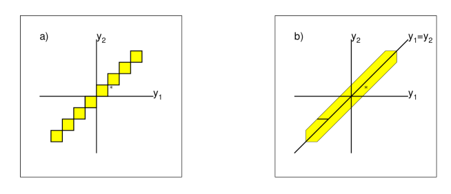
Figure 1: Integration domains for a) the second-order factorial moment and b) the second-order correlation integral. The asterisk in a) indicates the position of a particle pair with $|y_{1}-y_{2}|<\delta y$ that is excluded from the $F_{2}$ calculation due to the binning. In b) the asterisk is included.

Likewise, cell-averaged normalized factorial cumulant moments may be defined as

$$K_{q}(\delta y)=\frac{1}{M(\delta y)^{q}}\sum^{M}_{m=1}\int\limits_{\delta y}\frac{C_{q}(y_{1},\ldots,y_{q})\prod^{q}_{i=1}dy_{i}}{(\bar{\rho}_{m})^{q}}\ \ .$$ (16)

They are related to the factorial moments by 

$$F_{2} = 1+K_{2}\ \ \ ,$$

$$F_{3} = 1+3K_{2}+K_{3}\ \ \ ,$$

$$F_{4} = 1+6K_{2}+3\overline{K^{2}_{2}}+4K_{3}+K_{4}\,.$$ (17)

In $F_{4}$ and higher-order moments, “bar averages” appear defined as $\overline{AB}\equiv\sum\limits_{m}A_{m}B_{m}/M$.

To detect dynamical fluctuations in the density of particles produced in a high-energy collision, a way must be devised to eliminate, or to reduce as much as possible, the statistical fluctuations (noise) due to the finiteness of the number of particles in the counting cell(s). This requirement can to a large extent be satisfied by studying factorial moments and forms the basis of the factorial moment technique, known in optics, but rediscovered for multi-hadron physics in [7]. This crucial property does not apply to, e.g., ordinary moments $\langle n^{q}\rangle/\langle n\rangle^{q}$.

The property of Poisson-noise suppression has made measurement of factorial moments a standard technique, e.g. in quantum optics, to study the statistical properties of arbitrary electromagnetic fields from photon-counting distributions. Their utility was first explicitly recognized, for the single time-interval case, in [9] and later generalized to the multivariate case in [10].

2.4 Density and Correlation Integrals

A fruitful recent development in the study of density fluctuations is the correlation strip-integral method.[11] By means of integrals of the inclusive density over a strip domain of Fig. 1b, rather than a sum of the box domains of Fig. 1a, one not only avoids unwanted side-effects such as splitting of density spikes, but also drastically increases the integration volume (and therefore the statistical significance) at a given resolution.

Let us consider first the factorial moments $F_{q}$ defined according to Eq. 14. As shown in Fig. 1a for $q=2$, the integration domain $\Omega_{B}=\sum^{M}_{m=1}\Omega_{m}$ consists of $M$ $q$-dimensional boxes $\Omega_{m}$ of edge length $\delta y$. A point in the $m$-th box corresponds to a pair $(y_{1},y_{2})$ of distance $|y_{1}-y_{2}|<\delta y$ and both particles in the same bin $m$. Points with $|y_{1}-y_{2}|<\delta y$ which happen not to lie in the same, but in adjacent, bins (e.g., the asterisk in Fig. 1a) are left out. The statistics can be approximately doubled by a change of the integration volume $\Omega_{B}$ to the strip-domain of Fig. 1b. For $q>2$, the increase of integration volume (and reduction of squared statistical error) is in fact roughly proportional to the order of the correlation. The gain is even larger when working in two- or three-dimensional phase-space variables.

In terms of the strips (or hyper-tubes for $q>2$), the density integrals become

$$F^{\mathrm{S}}_{q}(\delta y)\equiv\frac{\int_{\Omega_{s}}\rho_{q}(y_{1}\dots y_{q}){\prod}_{i}{\mathrm{d}}y_{i}}{\int_{\Omega_{s}}\rho_{1}(y_{1})\dots\rho_{1}(y_{q}){\prod}_{i}{\mathrm{d}}y_{i}}\ \ .$$ (18)

These integrals can be evaluated directly from the data after selection of a proper distance measure $(|y_{i}-y_{j}|,[(y_{i}-y_{j})^{2}+(\phi_{i}-\phi_{j})^{2}]^{1/2}$, or better yet, the four-momentum difference $Q^{2}_{ij}=-(p_{i}-p_{j})^{2}$) and after definition of a proper multiparticle topology (GHP integral,[11] snake integral,[12] star integral [13]). Similarly, correlation integrals can be defined by replacing the density $\rho_{q}$ in Eq. 18 by the correlation function $C_{q}$.

The numerator of the factorial moments $F_{q}$ can be determined by counting, for each event, the number of $q$-tuples that have a pairwise $Q^{2}_{ij}$ smaller than a given value $Q^{2}$ and then averaging over all events. Using the Heaviside unit-step function ${\Theta}$, this can be mathematically expressed as

$$F^{\mathrm{S}}_{q}(Q^{2})=\frac{1}{\mbox{norm}}\left\langle q!\sum_{i_{1}<\dots<i_{q}}\prod_{all\ pairs\atop k_{1},k_{2}}{\Theta}(Q^{2}-Q^{2}_{i_{k_{1}},i_{k_{2}}})\right\rangle\ \ ,$$ (19)

where the factor $q$! takes into account the number of permutations within a $q$-tuple.

The normalization is obtained from ”mixed” events constructed by random selection of tracks from different events in a track pool. The multiplicity of a mixed event is taken to be a Poissonian random variable, thereby ensuring that no extra correlations are introduced. A correction factor is applied for the difference in average multiplicity of the Poissonian and the experimental distribution. The mixed events are treated in the same way as real events.

2.5 Power-Law Scaling

The technique proposed in [7] consists of measuring the dependence of the normalized factorial moments (or correlation integrals) $F_{q}(\delta y)$ as a function of the resolution $\delta y$. For definiteness, $\delta y$ is supposed to be an interval in rapidity, but the method generalizes to arbitrary phase-space dimension, as occurs with the use of $Q^{2}$.

As pointed out above, the scaled factorial moments enjoy the property of “noise-suppression”. High-order moments further act as a filter and resolve the large $n_{m}$ tail of the multiplicity distribution. They are thus particularly sensitive to large density fluctuations at the various scales $\delta y$ used in the analysis.

As proven in [7], a “smooth” (rapidity) distribution, which does not show any fluctuations except for the statistical ones, has the property of $F_{q}(\delta y)$ being independent of the resolution $\delta y$ in the limit $\delta y\to 0$. On the other hand, if dynamical fluctuations exist and $P_{\rho}$ is “intermittent”, the $F_{q}$ obey the power law

$$F_{q}(\delta y)\propto(\delta y)^{-\phi_{q}}\ ,\ \ (\delta y\to 0).$$ (20)

The powers $\phi_{q}$ (slopes in a double-log plot) are related [14] to the anomalous dimensions

$$d_{q}=\phi_{q}/(q-1)\ \ ,$$ (21)

a measure for the deviation from an integer dimension. Equation 20 is a scaling law since the ratio of the factorial moments at resolutions $L$ and $\ell$

$$R=F_{q}(\ell)/F_{q}(L)=(L/\ell)^{\phi_{q}}$$ (22)

only depends on the ratio $L/\ell$, but not on $L$ and $\ell$, themselves.

Figure 2: Correlation-integral method applied to NA22 hadron-hadron data [17, 19] in terms of a) ln $F^{\mathrm{S}}_{q}$ and b) $\ln K^{*}_{q}$ as a function of $-\ln Q^{2}$.

As pointed out above, the experimental study of correlations is already difficult for three particles. The close connection between correlations and factorial moments offers the possibility of measuring higher-order correlations with the factorial moment technique at smaller distances than was previously feasible. Via Eq. 21, the method further relates possible scaling behavior of such correlations to the physics of fractal objects.

One further has to stress the advantages of factorial cumulants compared to factorial moments, since the former measure genuine correlation patterns, whereas the latter contain additional large combinatorial terms which mask the underlying dynamical correlations.

The definition of “intermittency” given in (20), has its origin in other disciplines. It rests on a loose parallel between the high non-uniformity of the distribution of energy dissipation, for example, in turbulent intermittency and the occurrence of large “spikes” in hadronic multiparticle final states. In the following we use the term “intermittency” in a weaker sense, meaning the rise of factorial moments with increasing resolution, not necessarily according to a strict power law.

3 The State of the Art

The suggestion that normalized factorial moments of particle distributions might show power-law behavior has spurred a vigorous experimental search for (more or less) linear dependence of $\ln F_{q}$ on $-\ln\delta y$. A full review of the present situation is given in [16].

$\Delta F_{2}$

Figure 3: Comparison of density integrals for $q=2$ in their differential form $\Delta F_{2}$ (in intervals $Q^{2},Q^{2}+{\mathrm{d}}Q^{2}$) as a function of ${}_{2}\log(1/Q^{2})$ for e⁺e^- (DELPHI, preliminary) and hadron-hadron collisions (UA1).[20]

As an example, we give Fig. 2a where hadron-hadron data [17] on $F^{\mathrm{S}}_{q}$ are plotted as a function of $-\ln Q^{2}$, with all two-particle combinations in an $n$-tuple having $Q^{2}_{ij}<Q^{2}$. The following observations can be made: i)    the moments show a steep rise with decreasing $Q^{2}$; ii)   negatives are much steeper than all-charged, iii)  $F^{\mathrm{S}}_{2}$ is flatter for $(+-)$ than for all-charged or like-charged combinations.

The last two observations directly demonstrate the large influence of identical particle correlations on the factorial moments and their scaling behavior. These results agree very well with results from the UA1 collaboration.[18] In Fig. 2b it is, furthermore, shown [19] in terms of the $K^{*}_{q}(Q^{2})$ (using the star topology) that genuine correlations exist and increase with improving resolution at least up to order $q=5$ in hadron-hadron collisions. Again, like-charged particle combinations increase faster than all-charged ones.

Of particular interest is a comparison of hadron-hadron to e⁺e^- results in terms of same and opposite charges of the particles involved. This comparison has been done for UA1 and DELPHI data in [20] and is shown in Fig. 3 for $q=2$ (in fact, in this figure a differential form $\Delta F_{2}$ of Eq. 19 is presented). An important difference between UA1 and DELPHI can be observed in a comparison of the two sub-figures:

For relatively large $Q^{2}(>0.03$ GeV²), where Bose-Einstein effects do not play a major role, the e⁺e^- data increase much faster with increasing $-_{2}\log Q^{2}$ than the hadron-hadron results. For e⁺e^-, the increase in this $Q^{2}$ region is very similar for same and for opposite-sign charges.

At small $Q^{2}$, however, the e⁺e^- results approach the hadron-hadron results.

The authors conclude that for e⁺e^- annihilation at LEP at least two processes are responsible for the power-law behavior: Bose-Einstein correlation following the evolution of jets. In hadron-hadron collisions at present collider energies, the Bose-Einstein effects seem mostly relevant.

The exact functional form of $\Delta F_{2}$ or $\Delta K_{2}$ is derived from the data of UA1 [18, 21] and NA22,[17] again in its differential form, in Fig. 4. Clearly, the low-$Q$ data favor a power law in $Q$ over a (non-scaling) exponential, double-exponential or Gaussian law.

In Fig. 5, the NA22 results for two-, three- and four-particle Bose-Einstein correlations (equivalent to $\Delta F_{2}(Q^{2})$ are compared to a multi-Gaussian parametrization.[24] In the conventional linear presentation of Fig. 5a the fits look reasonable. If the same data and same fits are presented in a log-log scale, however, the power-law deviation from the multi-Gaussians starts to become visible (Fig. 5b).

Figure 4: Density integral $\Delta F_{2}$ as a function of log $Q^{2}$ for NA22 [17], correlation integral $\Delta K_{2}$ as a function of log $Q$ for like-charged pairs in UA1 (preliminary) [21] compared to power-law, exponential, double-exponential and Gaussian fits, as indicated.

Figure 5: The normalized two-, three- and four-particle inclusive densities (equivalent to $\Delta F_{q}$) as a function of $Q^{2}$ (left) and $-\ln Q^{2}$ (right).[22] Curves show the multi-Gaussian fits according to [23].

If the observed effect is real, it supports a view recently developed in [24]. In that paper, intermittency is explained from Bose-Einstein correlations between (like-sign) pions. As such, Bose-Einstein correlations from a static source are not power-behaved. A power law is obtained if i) the size of the interaction region is allowed to fluctuate, and/or ii) the interaction region itself is assumed to be a self-similar object extending over a large volume. Condition ii) would be realized if parton avalanches were to arrange themselves into self-organized critical states.[25] Though quite speculative at this moment, it is an interesting new idea with possibly far-reaching implications. We should mention also that in such a scheme intermittency is viewed as a final-state interaction effect and is therefore not troubled by hadronization effects.

In perturbative QCD, on the other hand, the fractal structure of jets follows, in principle, from parton branching and the intermittency indices $\phi_{q}$ are directly related to the anomalous multiplicity dimension $\gamma_{0}=(6\alpha_{s}/\pi)^{1/2}$ [26, 27, 28, 29] and, therefore, to the running coupling constant $\alpha_{s}$ via the simple relation,

$$\phi_{q}=(q-1)D-\frac{q^{2}-1}{q}\gamma_{0}\ ,$$

where $D$ is the usual topological dimension of the analysis. In the same theoretical context, it has been argued [27, 28, 29] that the opening angle between particles is a suitable and sensitive variable to analyze and well suited for these first analytical QCD calculations of higher-order correlations. It is, of course, closely related to $Q^{2}$.

A first analytical QCD calculation [27] is based on the double-log approximation (DLA) with angular ordering [30] (for a recent experimental study of angular ordering see [31]) and on local parton-hadron duality.[32] A preliminary comparison with DELPHI data [33] gives encouraging results, but shows that the situation is far from trivial, since finite-energy effects, four-momentum cut-offs, resonance decays etc. still dominate at LEP energies.

4 Summary

Multiparticle production in high-energy collisions is an ideal field to study genuine higher-order correlations. Methods also used in other fields are being tested and extended here for general application. Indications for genuine, approximately self-similar higher-order correlations are indeed found in hadron-hadron collisions, but still need to be establised in their genuine and self-similar character in e⁺e^- collisions at high energies. At large four-momentum distance $Q^{2}$, they are not only expected to be an inherent property of perturbative QCD, but are directly related to the anomalous multiplicity dimension and, therefore, to the running coupling constant $\alpha_{s}$. At small $Q^{2}$, the QCD effects are complemented by Bose-Einstein interference of identical mesons carrying information on the unknown space-time development of particle production during the collision. The interplay between these two mechanisms, particularly important for an understanding of the process of hadronization, is completely unknown at the moment.

References

References

- [1] T.N. Thiele in The Theory of Observation, Ann. Math. Stat. 2 165 (1931).
- [2] R. Kubo, J. Phys. Soc. Japan 17, 1100 (1962).
- [3] B. Kahn, G.E. Uhlenbeck, Physica 5, 399 (1938).
- [4] K. Huang in Statistical Mechanics, John Wiley and Sons, 1963.
- [5] A.H. Mueller, Physics Review D 4, 150 (1971).
- [6] M.G. Kendall and A. Stuart in The Advanced Theory of Statistics, Vol. 1, C. Griffin and Co., London 1969.
- [7] A. Białas and R. Peschanski, Nucl. Phys. B 273, 703 (1986); ibid. B 308, 857 (1988).
- [8] P. Carruthers, H.C. Eggers and I. Sarcevic, Phys. Lett. B 254, 258 (1991).
- [9] G. Bédard, Proc. Phys. Soc. 90, 131 (1967).
- [10] D. Cantrell, Phys. Rev. A 1, 672 (1970).
- [11] H.G.E. Hentschel and I. Procaccia, Physica D 8, 435 (1983); P. Grassberger, Phys. Lett. A 97, 227 (1983); I.M. Dremin, Mod. Phys. Lett. A 13, 1333 (1988); P. Lipa, P. Carruthers, H.C. Eggers and B. Buschbeck, Phys. Lett. B 285, 300 (1992).
- [12] P. Carruthers and I. Sarcevic, Phys. Rev. Lett. 63, 1562 (1989).
- [13] H.C. Eggers et al., Phys. Rev. D 48, 2040 (1993).
- [14] P. Lipa and B. Buschbeck, Phys. Lett. B 223, 465 (1989); R. Hwa, Phys. Rev. D 41, 1456 (1990).
- [15] Ya.B. Zeldovich, A.A. Ruzmaikin, D.D. Sokoloff in The Almighty Chance, World Scientific Lecture Notes in Physics, Vol. 20 (World Scientific Singapore, 1990).
- [16] E.A. De Wolf, I.M. Dremin, W. Kittel, Phys. Reports 270 (1996) 1.
- [17] N. Agababyan et al., NA22 Coll., Z. Phys. C 59, 405 (1993).
- [18] N. Neumeister et al., UA1 Coll., Z. Phys. C 60, 633 (1993).
- [19] N.M. Agababyan et al., NA22 Coll., Z. Phys. B 332, 458 (1994).
- [20] F. Mandl and B. Buschbeck in Proc. Cracow Workshop on Multiparticle Production, Krakow, eds. A. Białas et al. (World Scientific, Singapore, 1994) p.1.
- [21] H. Eggers in Proc. 7th Int. Workshop on Multiparticle Production Correlations and Fluctuations, Nijmegen, eds. R. Hwa et al. (World Scientific, Singapore, to be publ.).
- [22] N.M. Agababyan et al., NA22 Coll., Z. Phys. C 68, 229 (1995) andW. Kittel in Proc. XXVIth Int. Symp. on Multiparticle Dynamics, Faro, eds. J. Dias de Deus et al., (World Scientific, Singapore, to be publ.).
- [23] M. Biyajima et al., Progr. Theor. Phys. 84, 931 (1990).
- [24] A. Białas, Acta Phys. Pol. B 23, 561 (1992).
- [25] P. Bak, C. Tang and K. Wiesenfeld, Phys. Rev. Lett. 59, 381 (1987); P. Bak and K. Chen, Sci. Am. 264, 46 (1991).
- [26] G. Gustafson and A. Nilsson, Z. Phys. C 52, 533 (1991).
- [27] W. Ochs and J. Wosiek, Phys. Lett. B 289, 159 (1992); ibid. 305, 144 (1993); Z. Phys. C 68, 269 (1995).
- [28] Y.L. Dokshitzer and I.M. Dremin, Nucl. Phys. B 402, 139 (1993).
- [29] Ph. Brax, J.-L. Meunier and R. Peschanski, Z. Phys. C62, 649 (1994).
- [30] B. I. Ermolaev and V. S. Fadin, JETP Lett. 33, 269 (1981); A. H. Mueller, Phys. Lett. B 104, 161 (1981); A. Bassetto, M. Ciafaloni, G. Marchesini and A. H. Mueller, Nucl. Phys. B 207, 189 (1982); G. Marchesini and B. R. Webber, Nucl. Phys. B 238, 1 (1984).
- [31] M. Acciari et al., L3 Coll., Phys. Lett. B 353, 145 (1995).
- [32] Ya. I. Azimov, Yu. L. Dokshitzer, V. A. Khoze and S. I. Troyan, Z. Phys. C 27, 65 (1985).
- [33] B. Buschbeck, P. Lipa, F. Mandl in Proc. 7th Int. Workshop on Multiparticle Production, “Correlations and Fluctuations”, Nijmegen, eds. R.C. Hwa et al. (World Scientific, Singapore, to be published).