WUB 96-43
HEAVY QUARK PHYSICS ON THE LATTICE

Abstract

We illustrate the current status of heavy quark physics on the lattice. Special emphasis is paid to the question of systematic uncertainties and to the connection of lattice computations to continuum physics. Latest results are presented and discussed with respect to the progress in methods, statistical accuracy and reliability.

1 Introduction

The role of lattice QCD in the field of heavy quark physics is twofold.

First of all it provides experimental and phenomenological physicists with reliable predictions of those non-perturbative QCD parts, which are in nature almost inevitably connected to most of the important electroweak processes. For example, the Cabbibo-Kobayashi-Maskawa matrix elements for the weak decay of the $b$ quark cannot be extracted from experimentally measured B meson decays without distinct knowledge about QCD bound state properties of heavy light systems, i.e. the form factors.

Secondly, in the heavy quark regime lattice QCD can successfully describe ”pure QCD” quantities like quarkonia splittings and the heavy quark potential, which, in turn, can be used to determine the strong running coupling constant $\alpha_{s}$.

In order to judge on the quality of results from lattice QCD it is necessary to understand roughly how the lattice method works in practice, what are its advantages and shortcomings, where systematic uncertainties originate from and how these uncertainties can be controlled.

In principle, the lattice procedure consists in solving the QCD path integral on a (Euclidean) space time lattice. The connection with continuum physics is made in the limit, where (a) the lattice constant $a$ goes to zero, and (b) the lattice volume $V$ goes to infinity. If it were possible to achieve this limit unambiguously, QCD would be solved.

In practice, however, the path integral can be evaluated only for finite values of $a$ and $V$. This is done numerically with the help of Monte Carlo methods, which introduce a statistical uncertainty on the results. In order to achieve the continuum limit, extrapolations in $a$ and $V$ are necessary. On top of this, most of the lattice calculations in the past have been performed in the so called quenched approximation, where (roughly speaking) internal fermion loops are neglected.

Progress in lattice QCD therefore has to be measured in terms of

• Statistical significance

• Reliability of the extrapolation $a\rightarrow 0$, $V\rightarrow\infty$

• Ability to include internal fermion loops.

Especially in the case of heavy-light systems, item (b) confronts lattice QCD with a serious problem. The inverse of the lattice constant $a^{-1}$ can be viewed as a (gauge invariant) cutoff to all lattice observables. With todays computer facilities, cutoffs up to $a^{-1}\simeq 3.5\mbox{GeV}$ can be achieved for suitably large lattice volumes. If one would try to calculate B-meson properties , with $M_{B}\simeq 5GeV$, directly on such a lattice, severe finite cutoff effects would prevent a reliable extrapolation $a\rightarrow 0$.

An obvious way to alleviate this problem is of course to extrapolate lattice data in mass from far below the cutoff into the region of heavy masses, e.g. to $M_{B}$. However, as the functional dependence of the lattice data on the heavy quark mass is in general not exactly known, this procedure introduces additional systematic errors, which need to be controlled.

In order to overcome this unsatisfactory situation, several methods have been developed and improved over the recent years. These methods can be classified into three different groups: a priori methods, phenomenological methods, and effective methods.

A priori methods trie to improve on the discretization of the QCD action in such a way, that cutoff effects are reduced. Those ”improved actions” converge faster to the correct continuum form, leaving the QCD physics unchanged. The most prominent example in this group is the Sheikholeslami-Wohlert action[3], which is often called clover action. In contrast to the standard Wilson action[4], finite cutoff effects proportional to $a$ are absent, at least on the classical level. It turns out, however, that quantum fluctuations can re-introduce $O(a)$ cutoff effects. This problem is currently tackled by a proper adjustment of the coefficient of the (additional) clover term. Lattice actions which include this adjustment are traded under the names ”tadpole improved clover action”[5] or ”non-perturbatively improved clover action”[6].
In principle it should be possible to formulate a ”perfect” lattice action, which is free of any cutoff effect. The construction of such an action is currently under consideration[7].

The basic idea of phenomenological methods is, to reduce finite cutoff effects by proper adjustment of lattice observables. This is achieved by a change in the normalization of the lattice quark propagator (LMK I)[8] and by a redefinition of the particle masses (LMK II)[9]. As the modifications are not implemented on a fundamental level, it is not clear whether this method leads to a general improvement of all lattice observables.

Effective methods have been designed for heavy quarks on the lattice. The idea is to remove the largest scale, i.e. the heavy quark mass, from the lattice action. If all remaining scales are small compared to the lattice cutoff, finite $a$ effects should be reduced substantially. Lattice implementations of effective methods have been developed for (a) the static approximation[10], i.e. the zeroth order of heavy quark effective theory, and (b) the non-relativistic QCD[11] (NRQCD). The latter approach starts from a non-relativistic approximation of QCD and includes, similar to the well known Fouldy-Wouthusen transformation, successively relativistic corrections in form of a $1/M_{Q}$ expansion. Clearly, the range of validity of such methods is limited to the region of (very) heavy quarks.

In view of the variety of all these methods, whose merits in some cases have not been fully proven yet, one could argue that lattice QCD has lost its status of being an ab initio method. In the following we will try to convince you of the opposite.

The backbone of large scale lattice calculations is always a powerful computer. The strong increase in sustained computer speed over the recent years allowed for a substantial improvement on statistical significance of lattice data as well as for a variation of the lattice constant and the lattice volume over a much larger range. With such a tool in hands, one can indeed check on the benefit of the different methods and calculate a reliable estimate of the size of systematic uncertainties. For example, one can measure the size of finite cutoff effects by performing a series of lattice simulations with different lattice constants $a$. In that view, the computer can be compared with the accelerator and the detector of a large experiment: the quality of the device has an decisive influence on the quality of the results.

In the following the actual status of the ”lattice experiments” within the field of heavy quark physics is reviewed in form of selected examples. We will discuss the decay constant of the $B$ meson, $f_{B}$, the semileptonic decays of $B$ mesons, and the determination of $\alpha_{s}$ from quarkonium splittings and the heavy quark potential.

2 Status of $f_{B}$

2.1 Strategy

The decay constant of the $B$ meson, $f_{B}$, is defined in the space time continuum by

$$\langle 0|A_{0}|B\rangle^{cont}\equiv m_{B}f_{B}\quad,$$ (1)

where $A_{0}$ denotes the zeroth component of the axial current and $m_{B}$ is the $B$ meson mass. Thus, $f_{B}$ can be determined once the matrix element on the left hand side of eq.(1) is known.

On the lattice, one calculates $\langle 0|A_{0}|B\rangle^{latt}$, which is related to its pendant in the continuum by

$$\langle 0|A_{0}|B\rangle^{cont}=Z_{A}\langle 0|A_{0}|B\rangle^{latt}\;.$$ (2)

The renormalization constant $Z_{A}$ accounts for the non-conservation of the axial current. Both, $\langle 0|A_{0}|B\rangle^{latt}$ and $Z_{A}$ depend on the lattice spacing $a$, and much work has been devoted to the problem of choosing $Z_{A}$ such that it just cancels the finite cutoff effects of the above product[12, 13]. As a satisfactory solution to this problem has not been found yet, an extrapolation $a\rightarrow 0$ is still necessary.

Figure 1: MILC collaboration[19]: $f_{Qq}\sqrt{M_{Qq}}$ vs. $1/M_{Qq}$ at a finite value of the cutoff ($a^{-}1\simeq 3.2\mbox{GeV}$). The solid line is a quadratic fit to the octagons ( ”heavier heavies” + static); the dashed line is a quadratic fit to the crosses (”lighter heavies” +static). The difference of the two curves in the heavy quark region illustrates the quality of the interpolation.

Due to limitations in computer time – and computer memory size – the $B$ meson mass is beyond currently attainable lattice cutoffs. Therefore, one calculates $f_{PS}$ with meson masses below the cutoff and in the static limit. An $1/m_{PS}$ expansion then interpolates between these results, yielding $f_{B}$ at a given value of the lattice cutoff. The quality of such an interpolation is demonstrated in fig.1.

This procedure has to be repeated for several cutoff values, and finally the continuum extrapolation $a\rightarrow 0$ has to be performed.

As an alternative to this standard procedure, one can in principle use the NRQCD effective method. Unfortunately, NRQCD is a non-renormalizable theory and one cannot send $a\rightarrow 0$. Therefore, one needs good control over discretization errors of the NRQCD action. In the end it is necessary to verify, that the results from the standard method and from NRQCD are consistent.

2.2 Results

Three years ago, the first calculation, which includes the $a\rightarrow 0$ extrapolation, has been performed by the PSI-WUPP collaboration[17]. In this simulation, the cutoff and the lattice volume were varied in the ranges $1.5\mbox{GeV}\leq a^{-1}\leq 3.0\mbox{GeV}$ and $1.0\mbox{fm}\leq V\leq 1.5\mbox{fm}$ respectively. The continuum extrapolation yielded $f_{B}=180(50)$MeV.

This year, the lattice determination of $f_{B}$ has been improved by large scale simulations of the JLQCD group[18] and the MILC collaboration[19]. Preliminary results of a NRQCD calculation of $f_{B}$ have been published by the SGO collaboration[20].

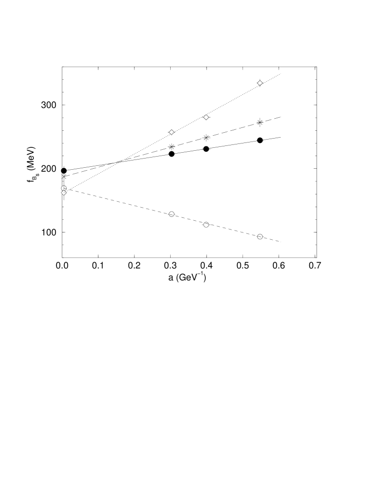
Figure 2: JLQCD collaboration[18]: $f_{B_{s}}$ as a function of the lattice spacing $a$. Different symbols refer to different choices of $Z_{A}$: naive (open circles), KLM (open diamonds), KLM improved (crosses), mixed KLM (filled circles).

JLQCD has pushed forward in the size of cutoff and volume, namely $1.8\mbox{GeV}\leq a^{-1}\leq 3.4\mbox{GeV}$ and $1.7\mbox{fm}\leq V\leq 2.0\mbox{fm}$. An important ingredient of their analysis is a careful study of the influence of different choices of $Z_{A}$ on the cutoff dependence of $f_{B}$. The result is displayed in fig.2. It turns out that, although none of the choices of $Z_{A}$ removes the cutoff dependence completely, the continuum values agree within errors. The remaining systematic uncertainty due to $Z_{A}$ can be read off the spread of results at $a=0$. The final JLQCD results read

$$f_{B}=179(11)^{+2}_{-31}\mbox{MeV}\qquad f_{B_{s}}=197(7)^{+0}_{-35}\mbox{MeV}\;.$$

The first error accounts for statistical, the second for systematic uncertainties. It is very encouraging to see the PSI-WUPP result being consolidated by the – more accurate – JLQCD calculation.

Figure 3: MILC collaboration[19]: $f_{B_{s}}$ as a function of the lattice spacing $a$. Octagons refer to quenched data; crosses to full QCD, $n_{f}=2$. The solid line is a fit to all quenched points (conf. level = 0.66); the dashed line is a constant fit to the three quenched points with $a<0.5\mbox{GeV}$ (conf. level = 0.76). The extrapolated values at $a=0$ are indicated as bursts.

The MILC collaboration has extended the cutoff even further. Their largest value is $a^{-1}\simeq 4.5\mbox{GeV}$. Fig.3 shows the final data as well as the extrapolation to $a=0$. For the first time in lattice QCD, MILC has been able to include full QCD simulations – with $n_{f}=2$ dynamical flavors – into the determination of $f_{B}$. The corresponding data is represented by crosses in fig.3. For small $a$ the full QCD data seem to enhance the value of $f_{B}$. However, the statistical uncertainty is too large to draw a firm conclusion. Instead, MILC quotes the quenched result and includes the effect of dynamical fermions as a systematic uncertainty

$$f_{B}=166(11)(28)(14)\mbox{MeV}\qquad f_{B_{s}}=181(10)(36)(18){MeV}\;.$$

The first error includes statistical errors and systematic effects of changing fitting ranges, the second other systematic errors within the quenched approximation, and the third accounts for quenching effects. Within errors, the MILC result is well compatible with PSI-WUPP and JLQCD.

The SGO collaboration has analyzed $n_{f}=2$ full QCD configurations, using NRQCD for the heavy quark. They quote a (preliminary) value of $f_{B}\simeq 180\mbox{MeV}$.

In summary, the ”old” value $f_{B}=180(50)\mbox{MeV}$ has been consolidated by more advanced lattice simulations. However, much work remains to be done in order to reduce statistical and systematic uncertainties. A major goal of the next years will be the inclusion of dynamical fermion loops.

3 Semileptonic Decays of $B$ Mesons

Semileptonic decay amplitudes can be described as a product of a (perturbatively accessible) weak interaction term and perturbatively not accessible QCD part. The latter is commonly parameterized by a set of form factors[21]

$$\langle\mbox{PS'}|J_{\mu}|\mbox{PS}\rangle = \mbox{Expr}\left\{f^{+}(q^{2}),f^{0}(q^{2})\right\}$$ (3)

$$\langle\mbox{V}|J_{\mu}|\mbox{PS}\rangle = \mbox{Expr}\left\{V(q^{2}),A_{1}(q^{2}),A_{2}(q^{2}),A(q^{2})\right\}\;.$$

PS, PS’ and V are momentum dependent pseudo-scalar and vector meson states, and $J_{\mu}$ is the (axial-) vector current. Clearly, the contribution from lattice QCD is a determination of the form factors by a calculation of the left hand side of eq.(3). Compared to the calculation of $f_{B}$ this is not an easy task, as both, the mass dependence and the $q^{2}$ behavior has to be determined. Due to limited statistical accuracy, it is not yet possible to extract the functional behaviors unambiguously from the data. Thus, systematic uncertainties due to the choice of inter- and extrapolation methods have to be estimated and finally included into the results.

3.1 $B\rightarrow\pi,\rho$

Considerable progress with respect to the reliability of inter- and extrapolations has been achieved within the last two years. ”Old” methods[22, 23], simply relied on the validity of the pole dominance hypothesis and on HQET. As the latter is justified only in the region $q^{2}\simeq q^{2}_{\mbox{max}}$ one had to operate at very large values of $q^{2}$.

As current lattice investigations substantially improved on the statistical quality of data, it has become possible to work at more moderate $q^{2}$ values and to check on the influence of the various assumptions.

The Wuppertal group[24] has performed its analysis at small values of $q^{2}$ and for meson masses up to $M_{D}$. In this region the form factors can be determined quite reliably. The extrapolation in mass

Figure 4: Wuppertal group[24]: Mass dependence of form factors $F(q^{2}=0)$ for the decays $B\rightarrow\pi$ and $B\rightarrow\rho$. Crosses denote the data. The solid line refers to a fit to $F=a_{1}+\frac{b_{1}}{M_{PS}}$ (a), the dashed line to $F=\frac{1}{\sqrt{M_{PS}}}\left(a_{2}+\frac{b_{2}}{M_{PS}}\right)$ (b), and the dotted line to $F=\sqrt{M_{PS}}\left(a_{3}+\frac{b_{3}}{M_{PS}}\right)$ (c). The extrapolated results are depicted at $1/m_{B}[\mbox{GeV}^{-1}]$ as filled circles (method a), upper triangles (method b), and stars (method c).

was done considering various parameterizations for the mass dependence, as shown in fig.4. Unfortunately the data is still not precise enough to discriminate between the Ansätze. However, the systematic uncertainty due to the extrapolation in mass can be estimated from the variation of results with respect to the various Ansätze.

An analysis which is more guided by the Heavy Quark Effective Theory (HQET) has been performed by the UKQCD[25] collaboration. In order to extract the maximal information from the data, they work at both, small and large values of $q^{2}$, combining the results after extrapolation to $M_{B}$. Although this method assumes the validity of HQET at moderate meson masses, e.g. at the $D$ meson mass, it leads to quite definite conclusions on the $q^{2}$ dependence of form factors at the $B$ meson mass.

Table 1: Form factors at $q^{2}=0$ for the semileptonic decays $B\rightarrow\pi(l\nu)$, $B\rightarrow\rho(l\nu)$

	$f_{+}(0)$	$f_{0}(0)$	$V(0)$	$A_{1}(0)$	$A_{2}(0)$
UKQCD[25]	$0.24^{+4}_{-3}$	$0.24^{+4}_{-3}$		$0.27^{+7}_{-4}\pm 3$	$0.28^{+9\;+4}_{-6\;-5}$
Wupp[24]	$0.50(14)^{+7}_{-5}$	$0.20(3)^{+2}_{-3}$	$0.61(23)^{+9}_{-6}$	$0.16(4)^{+22}_{-16}$	$0.72(35)^{+10}_{-7}$
APEa[23]	$0.29(6)$		$0.45(22)$	$0.29(16)$	$0.24(56)$
APEb[23]	$0.35(8)$		$0.53(31)$	$0.24(12)$	$0.27(80)$
ELCa[22]	$0.28(14)$		$0.37(14)$	$0.24(6)$	$0.39(24)$
ELCb[22]	$0.33(17)$		$0.40(16)$	$0.21(5)$	$0.47(28)$

Table 1 shows the results of the different groups. It turns out that the uncertainties are still too large to try a reliable extrapolation $a\rightarrow 0$.

3.2 $B\rightarrow D,D^{*}$

In order to estimate the systematic effects due to the various inter- and extrapolation methods, the Wuppertal group has applied the same type of analysis as for the decays $B\rightarrow\pi,\rho$.

In contrast, the UKQCD collaboration[26] has performed its analysis completely within the framework of HQET. One major conclusion of their work is, that non-perturbative ”power corrections” to the form factors are small in the mass region of $D$ and $B$ mesons.

Table 2: Branching ratios ($\%$) for exclusive semileptonic $B$ decays with a $D$ or $D^{*}$ final state

	$\bar{B}^{0}\rightarrow D^{+}l^{-}\nu$	$\bar{B}\rightarrow D^{*+}l^{-}\nu$
UKQCD	$1.5^{+4}_{-4}\pm 0.3$	$4.8^{+8}_{-9}\pm 0.5$
WUPP	$2.1(1.4)$
CLEO I	$1.8\pm 0.6\pm 0.3$	$4.1\pm 0.5\pm 0.7$
CLEO II		$4.49\pm 0.32\pm 0.39$
ARGUS	$2.1\pm 0.7\pm 0.6$	$4.7\pm 0.6\pm 0.6$
ALEPH		$5.36\pm 0.50\pm 0.76$

In table 2 the results for the branching ratios are compared to the measurements[27] of ARGUS, CLEO and ALEPH.

4 Quarkonia splittings and $\alpha_{s}$

Pure heavy quark systems like quarkonia provide an ideal laboratory to study (gluonic) inter quark forces. Lattice QCD is well prepared to work in this lab with tools like NRQCD and improved actions.

In order to demonstrate their quality, we compare in fig.5 the experimentally measured $\Upsilon$ spectrum with the lattice results[28]. Both, the NRQCD data and the results of the calculation with tadpole improved clover action are in good agreement with experiment, once dynamical fermions are included. This sets the stage to extract the strong coupling $\alpha_{s}$ from the inter quark forces in the heavy quark regime.

Figure 5: $\Upsilon$ spectrum (left) and spin splittings. The data has been compiled by J. Shigemitsu[28].

In principle, any lattice quantity which can be reliably expanded in powers of $\alpha$ can be used to define the strong coupling on the lattice. In quarkonia studies one commonly works with $\alpha_{P}$[30], which is defined by

$$-lnW_{1,1}=\frac{4\pi}{3}\alpha_{P}\left(\frac{3.4}{a}\right)[1-(1.19+0.07n_{f})\alpha_{P}]\;.$$ (4)

$W_{1,1}$ is the $1\times 1$ Wilson loop, which has to be measured on the lattice. In order to determine the momentum scale $Q=\frac{3.4}{a}$ of $\alpha_{P}$, the lattice cutoff $a^{-1}$ needs to be known. This is the point, where quarkonium physics enters: $a^{-1}$ can be extracted by comparing the measured $1S-2S$ or $S-P$ splittings with the lattice data. Finally, extrapolations in the number $n_{f}$ of dynamical flavours and in the mass of dynamical quarks $m_{q}$ have to be carried out, $n_{f}=0,2\rightarrow n_{f}=3$, $m_{q}\rightarrow m_{eff}=(m_{u}+m_{d}+m_{s})/3$. As a result of this procedure, the NRQCD collaboration quotes[31]

$$\alpha_{P}^{(n_{f}=3)}[8.2\mbox{GeV}]=\left\{\begin{array}[]{ll}0.1948(29)(11)(37)&\mbox{S - P splitting}\\ \\ 0.1962(41)(08)(40)&\mbox{1S - 2S splitting}\end{array}\right.\;,$$

where the first error accounts for statistical uncertainties, the second for discretization effects and the third for uncertainties due to the extrapolations. To compare with other determinations of the strong coupling it is advantageous to convert $\alpha_{P}$ to $\alpha_{\overline{MS}}$. Unfortunately, the corresponding two loop conversion formula has been calculated[32] hitherto only for $n_{f}=0$. This leads to an additional systematic uncertainty, which has to be taken into account. At the $M_{Z0}$ mass, the NRQCD collaboration finds[28]

$$\alpha_{\overline{MS}}[M_{Z0}]=\left\{\begin{array}[]{ll}0.1175(11)(13)(19)&\mbox{S - P splitting}\\ \\ 0.1180(14)(14)(19)&\mbox{1S - 2S splitting}\end{array}\right.\;.$$

Note that the last error, which accounts for the uncertainty in the conversion, dominates.

5 Summary and Conclusions

We have discussed the importance of recent developments and results in heavy quark physics on the lattice. Considerable progress has been achieved with respect to the reliability of the continuum extrapolation and to the inclusion of internal fermion loops. This is mainly due to the dramatic improvement in computer performance.

In order to reduce discretization effects, a variety of promising new ideas and methods has been developed. With the advent of fast parallel computers, the benefit of these methods can be tested reliably in numerical simulations. Once this has been done, they will be used for precise calculations at or even beyond the $b$ quark mass.

6 Acknowledgements

I thank Apoorva Patel for useful discussions.

References

- [1] M. Lüscher, P. Weisz, Phys. Lett. B158, (1985)250.
- [2] M. Alford et al., Nucl. Phys. B (Proc. Suppl.) 42, (1995)787.
- [3] B. Sheikholeslami, R. Wohlert, Nucl. Phys. B259 (1985)572.
- [4] K.G. Wilson, in New Phenomena in Subnuclear Physics, edited by A. Zichichi, Plenum, New York, 1977.
- [5] S. Collins et al., Nucl. Phys. B (Proc. Suppl.)47 (1996)366.
- [6] M. Lüscher et al.,Nonperturbative improvement of lattice QCD, CERN-TH-96-218, hep-lat 9609035; M. Lüscher et al., hep-lat 9608049, to be published in Nucl. Phys. B (Proc. Suppl.) 1997.
- [7] W. Bietenholz, U.J. Wiese, Nucl. Phys B464 (1996)319; W. Bietenholz et al., hep-lat 9608068, to be published in Nucl. Phys. B (Proc. Suppl.) 1997.
- [8] G.P. Lepage, P.B. Mackenzie, Phys. Rev. D48 (1993)2250; A.S. Kronfeld, Nucl. Phys. B (Proc. Suppl.) 30 (1993)445; P.B. Mackenzie, Nucl. Phys. B (Proc. Suppl.) 30 (1993)35.
- [9] A.S. Kronfeld, B.P. Mertens, Nucl. Phys B (Proc. Suppl.) 34 (1994)495; A.S. Kronfeld, Nucl. Phys. B (Proc. Suppl.) 42 (1995)415.
- [10] E. Eichten, Nucl. Phys. B (Proc. Suppl.) 4 (1988)170.; E. Eichten, Nucl. Phys. B (Proc. Suppl.) 20 (1991)475.
- [11] B.A. Thacker, G.P. Lepage, Phys. Rev D43 (1991)196; J.H. Sloan, Nucl. Phys. B (Proc. Suppl.) 42 (1995)171.
- [12] C.W. Bernard, Nucl. Phys. B (Proc. Suppl.) 34 (1994)47.
- [13] G. Martinelli et al., Nucl. Phys. B445 (1995)81.
- [14] C.W. Bernard, J.N. Labrenz, A. Soni, Phys. Rev. D49 (1994)2536.
- [15] R.M. Baxter et al., UKQCD collaboration, Phys. Rev. D49 (1994)1594.
- [16] O. Pene et al., Nucl. Phys. B (Proc. Suppl.) 26 (1992)344; A. Abada et al., Nucl.Phys. B376 (1992)172.
- [17] C. Alexandrou et al., Z. Phys. C62 (1994)659.
- [18] S. Aoki et al., JLQCD collaboration, hep-lat 9608142, to be published in Nucl. Phys. B (Proc. Suppl.) 1997.
- [19] C. Bernard et al., MILC collaboration, hep-lat 9608092, to be published in Nucl. Phys. B (Proc. Suppl.) 1997.
- [20] S. Collins, SGO collaboration, hep-lat 9608064, to be published in Nucl. Phys. B (Proc. Suppl.) 1997.
- [21] V. Lubicz, G. Martinelli, C.T. Sachrajda, Nucl. Phys. B356 (1991)301.
- [22] A. Abada et al., Nucl. Phys. B416 (1994)675.
- [23] C.R. Allton et al., APE collaboration, Phys. Lett B345 (1995)513.
- [24] S. Güsken, K. Schilling, G. Siegert, Nucl. Phys. B (Proc. Suppl.) 42 (1995)412.
- [25] D.R. Burford et al., UKQCD collaboration, Nucl. Phys. B447 (1995)425; J.M. Flynn et al., UKQCD collaboration, Nucl. Phys. B461 (1996)327; J.M. Flynn, J. Nieves, UKQCD collaboration, preprint SHEP 96-01, hep-ph 9602201.
- [26] K.C. Bowler et al., UKQCD collaboration, Phys. Rev. D52 (1995)5067; L. Lellouch, UKQCD collaboration, preprint CPT-95/P.3196, hep-ph 9505423.
- [27] T.E. Browder, K. Honscheid, Prog. Part. Nucl. Phys. 35 (1995)81, hep-ph 9503414.
- [28] J. Shigemitsu, HEP-LAT 9608058, to appear in Nucl. Phys. B (Proc. Suppl.)1997.
- [29] M. Lüscher et al., Nucl. Phys. B (Proc. Suppl.) 30 (1993)139.
- [30] G.P. Lepage, P.B. Mackenzie, Phys. Rev. D48 2250(1993).
- [31] C.T.H. Davies et al., Phys. Lett. B345,(1995)42; P. McCallum, J. Shigemitsu, Nucl. Phys. B (Proc. Suppl.) 47 (1996)409.
- [32] M. Lüscher, P. Weisz, Phys. Lett. B349 (1995)165.