UND-HEP-96-BIG 08

hep-ph/9612349

The Heavy Quark Expansion

Nikolai Uraltsev

TH Division, CERN, CH 1211 Geneva 23, Switzerland,

Dept. of Physics, Univ. of Notre Dame du Lac, Notre Dame, IN 46556, U.S.A.
and

Petersburg Nuclear Physics Institute, Gatchina, St.Petersburg 188350, Russia

Abstract

I review the status of the modern theoretical approach to weak decays of heavy flavor hadrons based on the $1/m_{Q}$ expansion in QCD. The qualitative features are explained and the subtleties in simultaneously incorporating perturbative and power-suppressed effects are addressed. A few topical phenomenological applications are discussed in quantitative detail.

1 Introduction

The Standard Model (SM) of fundamental interactions has so far yielded a consistent description of various experimental data; still, from the general perspective it is often viewed incomplete. A key role in exploring the SM is played by studying electroweak decays of heavy flavor particles. Unique information about the masses and mixing of quarks is obtained here thus setting the stage for addressing some of the most mysterious questions about the origin of the quark mixing and CP violation.

The fact that the dynamics of heavy flavor hadrons represents a peculiar field where the strong interaction effects allow a systematic treatment based on first principles of QCD, was realized already in the 70s. Yet, the full variety of theoretical tools available for gauge theories was applied here only over the last few years.

Two main directions were instrumental in developing QCD towards its current status of the theory underlying strong interactions: one was based on studying symmetry properties like isotopic or $SU(3)$ symmetry and chiral invariance; the second exploited the asymptotic freedom which allowed using dynamical calculations in the perturbative way for high-energy processes. These two approaches, the ‘symmetry-based’ and ‘dynamical’, are clearly seen in the evolution of the heavy quark theory.

During the early period to the end of the 80’s, most applications carried the ‘dynamical’ spirit and were done often at a somewhat simplified intuitive level. The nonperturbative effects typically were thought to be small even in the decays of charm particles. At the same time, the basic facts about the heavy quark spin and flavor symmetry were realized and incorporated to the necessary extent.

The symmetry considerations flourished for a few years with the formulation of the so-called Heavy Quark Effective Theory (HQET) which made these symmetries explicit at the level of the Lagrangian. It provided a convenient framework for discussing exclusive semileptonic or electroweak radiative decays and calculating basic perturbative corrections to them. On the other hand, the range of applications of HQET was limited, and not all virtues of the general Heavy Quark QCD Expansion (HQE) were employed.

Finally, over the last few years a consistent well-defined dynamical approach has been developed, which automatically respects the heavy quark symmetries in a manifest way. It has been realized that the nonperturbative corrections are often sizable even in the decays of beauty. Incorporating the actual dynamical calculations allowed one to make the most precise determinations of $|V_{cb}|$ and $|V_{ub}|$.

The main effects in a weak decay of a heavy quark $Q$ originate from distances $\sim 1/m_{Q}\ll 1/\Lambda_{\rm QCD}$. Belonging to the weak coupling domain, $\alpha_{s}(m_{Q})\ll 1$, they are tractable through perturbation theory. The QCD-interaction becomes strong only when the momentum transfer is much smaller than the heavy quark mass, $k\ll m_{Q}$. This simple observation elucidates the two basic ingredients of the heavy quark expansion that is genuinely based on QCD:

• The nonrelativistic expansion, which yields the effects of ‘soft’ physics in the form of a power series in $1/m_{Q}$.

• The treatment of the strong interaction domain based on the Operator Product Expansion (OPE).

Unless an analytic solution of QCD is at hand, these two elements appear to be indispensable for the heavy quark theory.

The necessity of separating the two domains characterized by momenta much larger than $\Lambda_{\rm QCD}$ and those which do not scale with $m_{Q}$, is thus manifest. The perturbative corrections, on the other hand, bridge the short-distance domain with the least understood domain of confining strong forces.

The general idea of separating two domains and applying different theoretical tools to them was formulated long ago by K. Wilson [1] in the context of problems in statistical mechanics; in the modern language, applied to QCD it is similar to lattice gauge theories. The treatment of essentially Minkowski quantities has, however, some peculiarities which attracted attention of theorists very recently.

The perturbative corrections – in spite of being often complicated technically – look straightforward from the conceptual viewpoint. On the contrary, getting even a minimal model-independent information about the nonperturbative physics often looks like a miracle. In view of the nature of this Symposium I will still try to put more accent onto the perturbative aspect, in particular, since the perturbative corrections got a renewed attention during the last two years. The overlap between the ‘perturbative’ and ‘nonperturbative’ effects is non-trivial indeed.

There are different technical ways to perform $1/m_{Q}$ expansion in QCD; the most popular schemes are known as the Nonrelativistic QCD (NRQCD) [2, 3] and the Heavy Quark Effective Theory (HQET) [4]. In what concerns the treatment of the perturbative corrections, in the standard HQET they are simply added to what is considered as the nonperturbative physics. On the other hand, the application of Wilson’s idea requires separating of any observable quantity into short-distance and long-distance pieces which, formally, is a different procedure. Schematically, the HQET decomposition

$$\mbox{An observable}\;=\;\mbox{perturbative piece}\;+\;\mbox{nonperturbative piece}$$

is replaced in Wilson’s OPE by a separation-scale–dependent representation

$$\mbox{An observable}\;=\;\mbox{short-distance piece}\;+\;\mbox{long-distance piece}\;\;.$$

The novel feature we face in the theoretical analysis of beauty decays nowadays is that they often allow – and even demand by virtue of the existence of precise experimental measurements – rather accurate predictions, requiring a simultaneous treatment of perturbative and nonperturbative QCD effects with the enough precision in both. This problem is not new; the theoretical framework has been elaborated more than 10 years ago [5], but its phenomenological implementation was not mandatory until recently. It is the exceptional beauty of the fifth quark that allows – in spite of interference of the nonperturbative effects – to make certain reliable theoretical predictions with errors at a percent level, which necessitates taking care of such ‘puristic’ theoretical subtleties. Nevertheless, failure to incorporate them properly, leads to certain theoretical paradoxes and, unfortunately, some superfluous controversy in the numerical estimates surfacing every now and then in the literature.

In spite of the significant progress made over the last years, the theory of the heavy flavors is not yet a completed field and is undergoing to further extensive development. There are quite a few topics which separately deserve a proper review:

• Sum rules for the weak transitions with the nonperturbative effects included. In a certain way they replace the quantum mechanical (QM) description in the field theory. The perturbative corrections to the sum rules were actively discussed, often with quite different conclusions.

• The so-called BLM-resummation and renormalons.

• The QCD-based OPE vs. ‘Fermi motion’ in heavy quark decays.

• The QCD sum rules calculations of the most interesting electroweak formfactors in the $b\rightarrow u$ ($b\rightarrow s$) transitions.

• Attempts to obtain constraints on the transition formfactors relying on the most general unitarity and analyticity properties. Without an actual dynamical input they are too weak, however. There is an interesting idea to incorporate additional constraints from lattice QCD.

• The heavy quark expansion for the production of heavy flavor hadrons and quarkonia.

The practical applications were in focus, too:

• Determination of $|V_{cb}|$ and $|V_{ub}|$.

• A model-independent extraction of $m_{b}$.

• Radiative corrections to ${\rm BR_{sl}}(B)$.

There is also a renewed interest in the inclusive nonleptonic widths.

Finally, the violations of duality is more and more discussed in the context of the heavy quark physics.

Even this, by necessity truncated, list gives a feeling of the extensive development taking place. Inevitably, I cannot cover here all, and even a large part of recent theoretical advances, or simply list all relevant references. A true measure of our understanding of the strong interaction dynamics is, eventually, determined by the theoretical accuracy with which we can extract the fundamental underlying parameters like the KM mixing angles from experimental data. Therefore, I will focus in this talk on a few selected topics that illustrate the theoretical framework used in the most accurate determination of the flavor mixing parameters, and review the overall status of the heavy quark expansion for beauty particles, with the main emphasis on the qualitative features.

2 Semileptonic decays

The QCD-based heavy quark expansion can in principle equally be applied to all types of heavy flavor transitions. Semileptonic decays, however, are the simplest case and I shall devote most of the attention to them. For practical reasons I focus on the $b\rightarrow c$ transitions; a brief discussion of the $b\rightarrow u$ decays will be given later.

A typical semileptonic decay is schematically shown in Figs. 1. Generally, two types of the decay rates can be singled out: the inclusive widths, where any combination of hadrons is allowed in the final state, and the exclusive decays, when a transition into a particular charmed hadron is considered, usually $D$ or $D^{*}$.

Figure 1: Exclusive $B\rightarrow D^{(*)}$ (a)   and generic (b)   semileptonic decays.

2.1 Inclusive semileptonic widths

The four-fermion semileptonic decay width of a heavy quark has the form

$$\Gamma_{\rm sl}=\frac{G_{F}^{2}m_{b}^{5}}{192\pi^{3}}|V_{cb}|^{2}\cdot z_{0}\left(\frac{m_{c}^{2}}{m_{b}^{2}}\right)\cdot\mbox{\ae}\;\;,$$ (1)

where $z_{0}$ is the known phase space suppression factor and æ generically includes all QCD corrections. In the heavy quark limit the difference resulting from using the quark mass $m_{b}$ and the meson mass $M_{B}$ in eq. (1) disappears:

$$\frac{M_{B}-m_{b}}{m_{b}}\;\sim\;\frac{1}{m_{b}}\;\;.$$ (2)

For the actual $b$ quark $m_{b}^{5}$ and $M_{B}^{5}$ differ by a factor of $1.5$–$2$, which formally constitutes a power-suppressed nonperturbative effect. This demonstrates the necessity of a systematic control of the nonperturbative corrections even in the decays of beauty particles.

The central result for the inclusive decay widths in QCD which is guaranteed by the application of the OPE to the heavy quarks in full QCD, is the absence of the $1/m_{Q}$ corrections [6, 7]. This seems non-trivial a priori since there are such corrections to the masses, in particular, differentiating masses of different types of hadrons ($\Lambda_{b}$, $B$, $B^{**}$). The physical reason behind this fact is the conservation of the color flow in QCD, that ensures the cancellation of the effects of the color charge (Coulomb) interaction in the initial and final states. In terms of nonrelativistic quantum mechanics it is the cancellation between the phase-space suppression caused by the Coulomb binding energy in the initial state, and the Coulomb distortion of the final state quark wavefunctions. The inclusive nature of the total widths leads to the fact that the width is sensitive only to the strong interaction on the time scale $\sim 1/\Delta E\sim 1/m_{b}$ ($\Delta E$ denotes the energy release). The final state interaction effect is thus not determined by the actual behavior of the strong forces at typical hadronic distances, but only by the potential in the close vicinity of the heavy quark; the cancellation occurs universally, whether or not a nonrelativistic QM description is applicable.

The leading power corrections start with terms $1/m_{b}^{2}$; they have been calculated in Ref. [6, 7] and are expressed in terms of the expectation values of two operators of dimension $5$, which in the language of QM are interpreted as the strength of the chromomagnetic field at the position of the heavy quark and the square of the spacelike momentum of the heavy quark jiggling in the rest-frame of the hadron, respectively:

$$\mu_{G}^{2}\simeq\frac{1}{2M_{B}}\langle B|\bar{b}\frac{i}{2}\sigma_{\mu\nu}G^{\mu\nu}b|B\rangle\leftrightarrow\langle B|\vec{\sigma}_{b}\cdot g_{s}\vec{{\cal H}_{g}}(0)|B\rangle\simeq\frac{3}{4}(M_{B^{*}}^{2}\!-\!M_{B}^{2})\simeq 0.35\,\mbox{GeV}^{2}$$ (3)

$$\mu_{\pi}^{2}\simeq\frac{1}{2M_{B}}\langle B|\bar{b}(i\vec{D}\,)^{2}b|B\rangle\leftrightarrow\langle B|\vec{p}^{\,2}|B\rangle$$ (4)

(the operators depend on the normalization point, but for simplicity I do not indicate this fact). The size of $\mu_{G}^{2}$ for $B$ mesons is derived from the observed hyperfine mass splitting between $B$ and $B^{*}$.

The value of $\mu_{\pi}^{2}$ is not yet known directly; a model-independent lower bound was established in [8, 9]

$$\mu_{\pi}^{2}\;>\;\mu_{G}^{2}\;\;,$$ (5)

which puts an essential constraint on its possible values. This bound is in agreement with QCD sum rule calculations [10], yielding a value about $0.5\,\mbox{GeV}^{2}$ and with an estimate [11] relying on the measured slope of the Isgur-Wise function. In the absence of the perturbative gluon corrections, as it happens, for example, in simple QM models, the expectation value of the kinetic operator $\mu_{\pi}^{2}$ would coincide with the HQET parameter $-\lambda_{1}$; they are different, however, in the actual field theory, where both $\mu_{\pi}^{2}$ and $\mu_{G}^{2}$ depend on the normalization point.

Including the nonperturbative corrections, the semileptonic width has the following form [6, 7, 12, 13]:

$$\Gamma_{\rm sl}=\frac{G_{F}^{2}m_{b}^{5}}{192\pi^{3}}|V_{cb}|^{2}\left\{z_{0}\left(1-\frac{\mu_{\pi}^{2}-\mu_{G}^{2}}{2m_{b}^{2}}\right)-2\left(1-\frac{m_{c}^{2}}{m_{b}^{2}}\right)^{4}\frac{\mu_{G}^{2}}{m_{b}^{2}}-\frac{2}{3}\frac{\alpha_{s}}{\pi}z_{0}^{(1)}+...\right\}$$ (6)

where ellipses stands for higher order perturbative and/or power corrections; $z$’s are known phase space factors depending on $m_{c}^{2}/m_{b}^{2}$. Irrespectively of the exact value of $\mu_{\pi}^{2}$, $\,1/m_{b}^{2}$ corrections to $\Gamma_{\rm sl}$ are rather small, about $-5\%$, thus leading to the increase in the extracted value of $|V_{cb}|$ by $2.5\%$; the impact of the higher order power corrections is negligible.

Good control of the QCD effects in the inclusive semileptonic widths provides the most accurate direct way to determine $|V_{cb}|$ in a truly model-independent way. This method sometimes faces a traditional scepticism: which numerical value must be used for $m_{b}$ and $m_{c}$? It appears that this practical problem has deep roots; failure to understand them is the major source of controversy about the heavy quark masses and inclusive widths often found in the literature. It will be briefly discussed below.

In reality the precise value of $m_{b}$ is not too important, since the $b\rightarrow c$ width depends to a large extent on the difference $m_{b}-m_{c}$ rather than on $m_{b}$ itself; the former is constrained in the heavy quark expansion

$$m_{b}-m_{c}=\frac{M_{B}+3M_{B^{*}}}{4}-\frac{M_{D}+3M_{D^{*}}}{4}+\mu_{\pi}^{2}\left(\frac{1}{2m_{c}}-\frac{1}{2m_{b}}\right)+...\approx 3.50\,\mbox{GeV}\;.$$ (7)

It also independently enters lepton spectra in semileptonic decays [13] and can be directly extracted from the data [14]. Numerically [8, 15], a change in $m_{b}$ by $50\,\mbox{MeV}$ leads only to a $1\%$ shift in $|V_{cb}|$.

Heavy quark masses

An accurate knowledge of the heavy quark mass becomes important if a few percent precision in $|V_{cb}|$ is targeted. However, rather different estimates of $m_{b}$ can be found in the literature. The reason is that the most popular scheme where certain features of the HQE were implemented, the HQET was based on the so-called pole mass of the heavy quarks. Not only was it a starting parameter of the HQET-based expansions, it is this pole mass that one always attempted to extract from the experimental data. It turns out, however, that the pole mass of the heavy quark is not a physical notion and cannot be even defined with the necessary accuracy in a motivated way: it suffers from an irreducible intrinsic theoretical uncertainty of order $\Lambda_{\rm QCD}$ [16]. This applies therefore to the parameter $\overline{\Lambda}=M_{B}-m_{b}^{\rm pole}$ as well.

At first sight this looks paradoxical and counter-intuitive: for the pole mass is a usual mass of a particle; for example, the value of $m_{\rm e}$ quoted in the tables of physical constants is just the pole mass of the electron. In QCD there is no ‘free heavy quark’ particle in the physical spectrum, and its pole mass is not well defined. The problems facing the possibilities to extract the pole mass from typical measurements were illustrated in Refs. [17] and [18].

The physical origin of the uncertainty $\delta m_{Q}^{\rm pole}\sim\Lambda_{\rm QCD}$ is the gluon Coulomb self-energy of the static colored particle. The energy stored in the chromoelectric field inside a sphere of radius $R\gg 1/m_{Q}$ is given by

$$\delta E_{\rm Coulomb}(R)\;\propto\;\int_{1/m_{b}\sim|x|<R}\;\vec{E}_{c}^{\,2}\;d^{3}x\;\;\propto\;\;{\rm const}-\frac{\alpha_{s}(R)}{\pi}\frac{1}{R}\;.$$ (8)

The pole mass assumes that all energy associated with the color source is counted, i.e. $R\rightarrow\infty$. Since in QCD the interaction becomes strong at $R_{0}\sim 1/\Lambda_{\rm QCD}$, the domain outside $R_{0}$ would yield an uncontrollable (and physically senseless) contribution to the mass $\sim\Lambda_{\rm QCD}$ [16].

Being a classical effect originating at a momentum scale well below $m_{Q}$, the appearance of this uncertainty can be traced in the usual perturbation theory, where it manifests itself in higher orders as a so-called $1/m_{Q}$ infrared (IR) renormalon singularity in the perturbative series for the pole mass [19, 20].

Figure 2: Perturbative diagrams leading to the IR renormalon uncertainty in $m_{Q}^{\rm pole}$ of the order of $\Lambda_{\rm QCD}$. The contribution of the gluon momenta below $m_{Q}$ expresses the classical Coulomb self-energy of the colored particle. The number of bubble insertions into the gluon propagator can be arbitrary.

To model the effect of the running coupling and emergence of the nonperturbative low-momentum domain one can use the running coupling $\alpha_{s}(k^{2})$ in the one-loop diagram for the correction to the on-shell mass of the heavy quark, see Fig. 2. In the nonrelativistic limit $k\ll m_{Q}$ the expression simplifies and reads

$$\delta m_{Q}\;\sim\;-\frac{4}{3}\,\int\;\frac{d^{4}k}{(2\pi)^{4}i}\>\frac{4\pi\alpha_{s}(k^{2})}{k^{2}}\,\frac{1}{k_{0}}\;=\;\frac{4}{3}\,\int\;\frac{d^{3}\vec{k}}{4\pi^{2}}\>\frac{\alpha_{s}(\vec{k}^{\,2})}{\vec{k}^{\,2}}\;.$$ (9)

Expanding running $\alpha_{s}(k^{2})$ in terms of a short-distance $\alpha_{s}(\mu^{2})$ one obtains for $\delta m_{Q}$ the whole series in $\alpha_{s}(\mu^{2})$. The coefficients grow factorially:

$$\frac{\delta m_{Q}}{m_{Q}}\;\sim\;\frac{4}{3}\,\frac{\alpha_{s}}{\pi}\,\left(\frac{b\alpha_{s}}{2\pi}\right)^{n}\,n!\;\;,\qquad\qquad\qquad b=\frac{11}{3}N_{c}-\frac{2}{3}n_{f}=9\;,$$ (10)

and the nonperturbative regime manifests itself as the uncertainty in defining a sum of such a series. Numerically, the calculation of the contribution of the domain below $\mu\simeq 1\,\mbox{GeV}$ would then look as follows:

$$m_{b}^{\rm pole}\;=\;m_{b}(1\,\mbox{GeV})+\delta m^{\rm pert}\;\simeq\;$$

$$4.55\,\mbox{GeV}+0.25\,\mbox{GeV}+0.22\,\mbox{GeV}+0.38\,\mbox{GeV}+1\,\mbox{GeV}+3.3\,\mbox{GeV}+14\,\mbox{GeV}+\>...$$ (11)

Clearly, such a possibility does not look encouraging if one really needs to know the heavy quark mass accurately enough!

The first two terms in eq. (11) constituting approximately $4.8\,\mbox{GeV}$ can be called – with some reservations [17] – the ‘one-loop’ pole mass that enters typical calculations when order-$\alpha_{s}$ corrections are computed. Recently, the third term was incorporated [21] in the analysis of the lepton spectra in the semileptonic $b$-decays and the value

$$\overline{\Lambda}\;=\;M_{B}-m_{b}^{\rm pole}\;\simeq\;(390\pm 110)\,\mbox{MeV}$$ (12)

was deduced. The quoted error, according to [21], includes “only experimental uncertainty” – however, such a numerical conclusion can hardly be taken sensibly.

In spite of this irreducible uncertainty in $m_{Q}^{\rm pole}$ and $\overline{\Lambda}$, the inclusive widths, though dependent on the mass, can be theoretically calculated since they are governed not by the pole masses, but well-defined short-distance running masses $m_{Q}(\mu)$ with the Coulomb energy originating from distances $\mathrel{\hbox to0.0pt{\lower 4.0pt\hbox{\hskip 1.0pt$\sim$}\hss}\raise 1.0pt\hbox{$>$}}1/\mu$ peeled off. Moreover, it is precisely this short-distance running mass rather than the pole mass that can be extracted from experiment with, in principle, unlimited accuracy: the pole mass does not enter any genuine short-distance observable at the level of nonperturbative corrections, which can be calculated by means of the OPE [19]. It is worth noting that the irrelevance of the pole mass roots deeper than merely the problem of the IR renormalon; even if there were no problem in defining the pole mass in QCD, its infrared part distinguishing it from the short-distance mass is still foreign to the OPE.

Applied to the inclusive widths, this observation suggests certain information about the importance of higher order perturbative corrections: if masses entering eq. (6) are the pole masses, the perturbative series

$$\Gamma_{\rm sl}^{\rm pert}=\Gamma_{0}\mbox{\ae}^{\rm pert}=\Gamma_{0}\left(1+a_{1}\frac{\alpha_{s}}{\pi}+a_{2}\left(\frac{\alpha_{s}}{\pi}\right)^{2}+...\right)$$ (13)

is poorly behaved, with coefficients $a_{k}$ factorially growing, which makes it non-convergent and the radiative correction factor per se uncalculable in principle either with an accuracy $\sim\Lambda_{\rm QCD}/m_{b}$. In contrast, if one uses the short-distance masses, the higher-order corrections become smaller and the overall factor is theoretically calculable with the necessary precision [19, 22].

This, at first glance rather academic, observation in reality proved to underlie the pattern of the corrections from the very first terms. Remarkably, the actual model-independent calculations of $\Gamma_{\rm sl}$ through observables measured in experiment are very stable against perturbative corrections. Including ${\cal O}(\alpha_{s}^{2})$ terms in the extraction of the $b$ pole mass from, say, the $\rm e^{+}e^{-}\rightarrow\bar{b}b$ threshold region [23] noticeably increases its value. However, if one performs the parallel perturbative improvement in calculating the width, one finds an essential suppression of the perturbative factor $\mbox{\ae}^{\rm pert}$. The two effects offset each other almost completely.

This conspiracy is not unexpected: the appearance of large corrections at both stages is merely an artefact of using the ill-defined pole mass in the intermediate calculations. The situation is peculiar since the actual nonperturbative effects appear only at the level $1/m_{Q}^{2}$, whereas the pole mass is infrared ill-defined already at an accuracy of $1/m_{Q}$. The failure to realize this fact led to a superficial suggestion [24] that even in beauty particles the perturbative corrections may go out of theoretical control; a more careful analysis [15, 25] showed that this is not the case.

Since the apparent troubles with the perturbative corrections are associated with the pole masses, it is better to get rid of them altogether using instead running masses $m_{b,c}(\mu)$ normalized at $\mu\sim 1\,\mbox{GeV}$; this is advantageous both theoretically and in practice. This has been done in [15] and showed that neither masses nor the perturbative corrections to the width $\mbox{\ae}^{\rm pert}$ have significant contributions from higher orders. It is important to note that it is not a kind of empirically selected procedure but is required in the literal implementation of Wilson’s OPE in the case of the heavy quark widths [19].

To summarize, the idea that the perturbative corrections in the extraction of $|V_{cb}|$ from $\Gamma_{\rm sl}(B)$ are large emerges from an attempt to use ill-defined pole masses in an inconsistent way where two problems are encountered:

• It is ‘difficult to extract’ accurately $m_{b}^{\rm pole}$ from experiment; in any particular calculation the effects are easily identified that were left out, which can change its value by $\sim 200\,\mbox{MeV}$. This uncertainty leads to a ‘theoretical error’ $\delta_{\rm I}$ in $\Gamma_{\rm sl}(B)$ of about $10\%$.

• When routinely calculating $\Gamma_{\rm sl}(B)$ in terms of the pole masses, there are significant higher order corrections $\delta_{\rm II}\simeq 10\%$.

The naive conclusion drawn from such experience [26] is that one cannot reliably calculate the width without $\sim 20\%$ uncertainty:

$$\frac{\delta\Gamma_{\rm sl}}{\Gamma_{\rm sl}}=\delta_{\rm I}+\delta_{\rm II}\simeq 20\%\;\;\leftrightarrow\;\;\frac{\delta|V_{cb}|}{|V_{cb}|}\simeq 10\%\;\;.$$

On the contrary, theory predicts a cancellation between $\delta_{I}$ and $\delta_{II}$ in a consistent perturbative calculation, and that was explicitly checked in [15, 25]. For example, the net impact of the calculated (presumably dominant) second-order ${\cal O}(\alpha_{s}^{2})$ corrections on the value of $|V_{cb}|$ appeared to be less than $1\%\,$! Moreover, just neglecting all perturbative corrections altogether, both in the semileptonic width and in extracting $m_{b}$ from experiment, yields a $|V_{cb}|$ smaller by less than $5\%$ [27].

Recently, all-order corrections associated with the effect of running of $\alpha_{s}$ in one-loop diagrams (I shall refer to it in what follows as an extended BLM, or, shorter, merely a BLM approximation) were calculated in [25], thus improving the exact one-loop result which has been known from the QED calculations [28]. Using the most accurate model-independent low-energy determination of $m_{b}$ [23] one gets [15]

$$|V_{cb}|=0.0413\left(\frac{{\rm BR}(B\rightarrow X_{c}\ell\nu)}{0.105}\right)^{\frac{1}{2}}\left(\frac{1.6\,\rm ps}{\tau_{B}}\right)^{\frac{1}{2}}\times$$

$$\left(1-0.012\frac{(\tilde{\mu}_{\pi}^{2}-0.4\,\rm GeV^{2})}{0.1\,\rm GeV^{2}}\right)\cdot\left(1-0.006\frac{\delta m_{b}^{*}}{30\,\rm MeV}\right)\;.$$ (14)

The relevant sources of theoretical uncertainty are shown explicitly. The main one is lack of knowledge of the exact value of $\mu_{\pi}^{2}$ (marked with a tilde in eq. (14) , indicating that a particular field-theoretic definition of the kinetic operator has been assumed), which enters through the value of $m_{b}-m_{c}$, eq. (7). A dedicated analysis of the lepton spectra will reduce this uncertainty. At the moment a reasonable estimate of the actual uncertainty in $\mu_{\pi}^{2}$ is about $0.2\,\mbox{GeV}^{2}$, leading to a $2.5\%$ uncertainty in $|V_{cb}|$.

The dependence on the absolute value of $m_{b}$ is minor; since we rely here on the well-defined short-distance mass $m_{b}^{*}$, there is no intrinsic uncertainty in its value. The analysis [23] estimated $\delta m_{b}^{*}\simeq 30\,\mbox{MeV}$ which seems reasonable; to be confident, I double it, and even then the related uncertainty in $|V_{cb}|$ is less than $1.5\%$.

Finally, we should consider the perturbative corrections. As previously explained, the actual impact of the known perturbative corrections when relating the semileptonic width to other low-energy observables is very moderate, and there is no reason to expect the higher-order effects to be significant. With the a priori dominant all-order BLM corrections calculated [25], one may be concerned only with the true two-loop effects ${\cal O}(\alpha_{s}^{2})$ which are not associated with the running of $\alpha_{s}$. These have not been calculated completely yet; however, the recent calculation [29] of the complete ${\cal O}(\alpha_{s}^{2})$ corrections in the small velocity kinematics demonstrated the feasibility of a complete calculation and suggested that the corrections must be small. There are some enhanced higher-order corrections not related to running of $\alpha_{s}$, that are specific to the inclusive widths [30]. They have been accounted for in the analyses [8, 15], but went beyond those in [31, 25]. With the results of [29] it seems unlikely that as yet uncalculated second-order corrections can change the width by more than $2$–$3\%$; therefore, assigning an additional uncertainty of $2\%$ in $|V_{cb}|$ is a quite conservative estimate.

Adding up these uncertainties we conclude that at present we can confidently calculate $|V_{cb}|$ from $\Gamma_{\rm sl}$ with the theoretical uncertainty

$$\frac{\delta|V_{cb}|}{|V_{cb}|}|_{\rm th}\;<\;5\%\;\;.$$ (15)

Keeping in mind some controversy about experimental value of ${\rm BR_{sl}}(B)$ and certain changes in time in $\tau_{B}$, it is fair to say that the theoretical accuracy in extracting $|V_{cb}|$ is even better than its current experimental counterpart.

It is important that this method has a potential for further improvement in a model-independent way. I think that the $2\%$ level of a defensible theoretical precision can be ultimately reached here. It is difficult to count on an essential improvement beyond that, because of impact of higher-order power corrections and possible violations of duality.

In a similar way it is straightforward to relate the value of $|V_{ub}|$ to the total semileptonic width $\Gamma(B\rightarrow X_{u}\,\ell\nu)$ [15]:

$$|V_{ub}|=0.00458\left(\frac{{\rm BR}(B\rightarrow X_{u}\ell\nu)}{0.002}\right)^{\frac{1}{2}}\left(\frac{1.6\,\rm ps}{\tau_{B}}\right)^{\frac{1}{2}}\;.$$ (16)

An accurate measurement of the inclusive $b\rightarrow u\,\ell\nu$ width is difficult and for a long time seemed unfeasible. However, recently ALEPH announced the first direct measurement [32]:

$${\rm BR}(B\rightarrow X_{u}\ell\nu)=0.0016\pm 0.0004\;\;.$$

I cannot judge the reliability of the quoted error bars in this complicated analysis; it certainly will be clarified in the future. Accepting the numbers literally, I arrive at the model-independent result

$$\frac{|V_{ub}|}{|V_{cb}|}\;=\;0.098\pm 0.013\;\;.$$ (17)

The theoretical uncertainty in translating $\Gamma(B\rightarrow X_{u}\,\ell\nu)$ into $|V_{ub}|$ is a few times smaller and is not seen in the final result.

To conclude this section on the inclusive semileptonic widths, let me briefly comment on the literature. It is sometimes stated that the existing uncertainty in $\Gamma_{\rm sl}$ is at least $20\%$ [26, 33]. The major origin of such claims is ignoring the subtleties related to using the pole mass in the calculations, and considering separately the perturbative corrections to the pole masses and to the widths expressed in terms of $m_{Q}^{\rm pole}$. This is inconsistent on theoretical grounds [19], whose relevance was confirmed by the concrete numerical evaluations of the BLM corrections in [15, 25]. The dependence on $m_{b}$ and $m_{b}-m_{c}$ used to determine the uncertainty in $|V_{cb}|$ was calculated erroneously in [26] (cf. [15]), apparently because of an arithmetic mistake that led to a significant overestimate. Finally, no convincing argument was given to justify a sevenfold boosting of the theoretical uncertainty in $m_{b}$ obtained in the dedicated analysis [23].

2.2 Exclusive zero-recoil $B\rightarrow D^{*}\,\ell\nu$ rate

Good theoretical control of all QCD effects in the inclusive widths was due to the fact that removing constraints on the final state to which decay partons can hadronize, makes such a probability a truly short-distance quantity amenable to a direct OPE expansion. Application of a similar idea to the exclusive zero-recoil decay rate $B\rightarrow D^{*}\,\ell\nu$ yielded quite an accurate determination of $|V_{cb}|$ as well [8, 17], though with a more significant irreducible model dependence and a larger intrinsic uncertainty. The limitation is twofold: first, constraining the decays to a specific final state makes the transition not a genuinely short-distance effect; second, it suffers from downgrading the expansion parameter, namely $1/m_{c}$ rather than $1/m_{b}$.

On the quark level the decay is shown in Fig. 1a; near zero recoil it is determined by the single hadronic formfactor $F_{D^{*}}$. In the absence of corrections violating the heavy quark symmetry, $F_{D^{*}}=1$ holds; for finite $m_{b,c}$ it acquires corrections:

$$F_{D^{*}}=1-(1-\eta_{A})+\delta_{1/m^{2}}+...\;\;.$$ (18)

The effect of the nonperturbative domain denoted by the last term and the ellipses starts with the terms $\sim 1/(m_{c},m_{b})^{2}$ [34, 35], but otherwise is rather arbitrary, since it depends on the details of the long-distance hadronization dynamics in the form of wavefunction overlap. This opened the field for speculations and certain controversy about the value of $F_{D^{*}}$ [36].

The situation as it existed by 1994 was summarized in the review lectures [37]:

$$\eta_{A}=0.986\pm 0.006\qquad\qquad\qquad\delta_{1/m^{2}}=(-2\pm 1)\%\qquad,$$ (19)

yielding $F_{D^{*}}\simeq 0.97$, and was assigned the status of “one of the most important and, certainly, most precise predictions of HQET”. Nowadays we believe that the actual corrections to the symmetry limit are larger, and the central theoretical value lies rather closer to $0.9$ [8, 17].

Regarding the perturbative calculations per se, it was later pointed out [38] that the improvement [39] of the original one-loop estimate was incorrect, and the proper value is rather $\eta_{A}\approx 0.965\pm 0.025$; subsequent calculations of the higher-order corrections in the BLM approximation [25, 40] confirmed it: $\eta_{A}\approx 0.965\pm 0.02$. The purely perturbative chapter was closed recently with the complete two-loop ${\cal O}(\alpha_{s}^{2})$ result [29]

$$\eta_{A}^{(\rm 2\,loop)}=0.960\pm 0.007\;\;.$$ (20)

It should be noted, however, that the inherent irreducible uncertainty of the complete perturbative series for $\eta_{A}$ exceeds the one stated in eq. (20) by a factor of three [25, 42, 43].

If the mass of the charm quark were a few times larger, from the practical viewpoint the two-loop calculation would have been the whole story for $F_{D^{*}}$. In reality, the power corrections originating from the domain of momenta below $\sim 0.6\,\mbox{GeV}$ appear to be more significant. Unfortunately, not much can be said about them in a model-independent way, although they have been shown to be negative and exceed about $0.04$ [8, 17] in magnitude (the analysis for $\Lambda_{b}$ was given in [44]).

The idea of this dynamical approach was to consider the sum over all possible hadronic states in the zero-recoil kinematics but not to limit it to only $B\rightarrow D^{*}$; such a rate sets an upper bound for the production of $D^{*}$. This inclusive quantity is of a short distance nature and can be calculated in QCD by means of the OPE. Schematically, the result through order $1/m^{2}$ is

$$|F_{D^{*}}|^{2}+\sum_{\epsilon_{i}<\mu}|F_{i}|^{2}=\xi_{A}(\mu)-\frac{\mu_{G}^{2}}{3m_{c}^{2}}-\frac{\mu_{\pi}^{2}-\mu_{G}^{2}}{4}\left(\frac{1}{m_{c}^{2}}+\frac{1}{m_{b}^{2}}+\frac{2}{3m_{c}m_{b}}\right)\;\;,$$ (21)

where $F_{i}$ are the-axial current transition formfactors to excited charm states $i$ with the mass $M_{i}=M_{D^{*}}+\epsilon_{i}$, and $\xi_{A}$ is a perturbative renormalization factor (the role of $\mu$ will be addressed later). Considering a similar relation for another type of ‘weak current’, say, $\bar{c}i\gamma_{5}b$, one obtains a different sum rule

$$\sum_{\tilde{\epsilon}_{k}<\mu}|\tilde{F}_{k}|^{2}=\left(\frac{1}{m_{c}}-\frac{1}{m_{b}}\right)^{2}\frac{\mu_{\pi}^{2}-\mu_{G}^{2}}{4}\;\;,$$ (22)

with the tilde referring to the quantities for the transitions induced by this hypothetical current. These sum rules (and similar ones at arbitrary momentum transfer), established in Refs. [8, 17], have been subjected to a critical scrutiny for two years, but are now accepted and constitute the basis for currently used estimates of $F_{D^{*}}$.

Since eq. (22) is the sum of certain transition probabilities, it is definite-positive and results in a rigorous lower bound

$$\mu_{\pi}^{2}\;>\;\mu_{G}^{2}\simeq 0.4\,\mbox{GeV}^{2}\;\;.$$ (23)

The sum rule (21) then leads to the model-independent lower bound for the $1/m^{2}$ terms in $F_{D^{*}}$:

$$-\delta_{1/m^{2}}\;>\;\frac{M_{B^{*}}^{2}-M_{B}^{2}}{8m_{c}^{2}}\simeq 0.035\;.$$ (24)

The actual estimate depends essentially on the value of $\mu_{\pi}^{2}$. It was suggested in [8] to estimate the contribution of the excited states in the l.h.s. of the sum rule (21) from $0$ to $100\%$ of the power corrections in the r.h.s.:

$$-\delta_{1/m^{2}}=(1+\chi)\left(\frac{M_{B^{*}}^{2}-M_{B}^{2}}{8m_{c}^{2}}+\frac{\mu_{\pi}^{2}-\mu_{G}^{2}}{8}\left(\frac{1}{m_{c}^{2}}+\frac{1}{m_{b}^{2}}+\frac{2}{3m_{c}m_{b}}\right)\right)\;,\;\;0\leq\chi\leq 1\;.$$ (25)

If so, one arrives at [8]

$$-\delta_{1/m^{2}}=(5.5\pm 1.8)\%\qquad\mbox{ at }\;\mu_{\pi}^{2}=0.4\,\mbox{GeV}^{2}$$

$$\,-\delta_{1/m^{2}}=(6.8\pm 2.3)\%\qquad\mbox{ at }\mu_{\pi}^{2}=0.5\,\mbox{GeV}^{2}\;\mbox{ }$$ (26)

$$-\delta_{1/m^{2}}=(8.1\pm 2.7)\%\qquad\mbox{ at }\;\mu_{\pi}^{2}=0.6\,\mbox{GeV}^{2}$$

Before proceeding to further phenomenological implications, let me dwell on the QM meaning of the sum rules [17]. The act of a weak semileptonic decay of the $b$ quark is its instantaneous replacement by $c$ quark. In ordinary QM the overall probability of the produced state to hadronize to some final state is exactly unity, which (neglecting radiative corrections) is the first, leading term in the r.h.s. of (21). Why then are there nonperturbative corrections in the sum rule? The answer is that the normalization of the weak current $\bar{c}\gamma_{\mu}\gamma_{5}b$ is not exactly unity and depends, in particular, on the external gluon field. Expressing the QCD current in terms of the nonrelativistic fields used in QM one has [17, 3], for example,

$$\bar{c}\gamma_{k}\gamma_{5}b\leftrightarrow\sigma_{k}-\left(\frac{1}{8m_{c}^{2}}(\vec{\sigma}i\vec{D})^{2}\sigma_{k}+\frac{1}{8m_{b}^{2}}\sigma_{k}(\vec{\sigma}i\vec{D})^{2}\;-\frac{1}{4m_{c}m_{b}}(\vec{\sigma}i\vec{D})\sigma_{k}(\vec{\sigma}i\vec{D})\right)+{\cal O}\left(\frac{1}{m^{3}}\right)$$ (27)

The last term just yields the correction seen in the rhs of the sum rule.

The inequality $\mu_{\pi}^{2}>\mu_{G}^{2}$ in QM expresses the positivity of the Pauli Hamiltonian

$$\frac{1}{2m}(\vec{\sigma}\,i\vec{D}\,)^{2}=\frac{1}{2m}\left((i\vec{D})^{\,2}-\frac{i}{2}\sigma G\right)$$

[9]. It is interpreted as the Landau precession of a charged (colored) particle in the (chromo)magnetic field where one has $\langle p^{2}\rangle\geq|\vec{B}|$. Literally, in $B^{*}$ the QM expectation value of the chromomagnetic field is suppressed, only $\mu_{G}^{2}/3$, and in $B$ it vanishes, since $\vec{B}$ is proportional to the spin of the light degrees of freedom. However, essentially non-classical nature of $\vec{B}$ (e.g., $\langle\vec{B}^{\,2}\rangle\geq 3\langle\vec{B}\rangle^{2}$) in turn enhances the bound which then takes the same form as in the external classical field.

Before returning to numbers, let me emphasize that the perturbative factor $\xi_{A}$ is not (and cannot be) equal to $\eta_{A}^{2}$ [17] (see also [19]). It is clear that purely perturbative calculations include (although in an improper way) the effect of the strong interaction domain completely described by the power terms. $\xi_{A}$ depends explicitly on the separation scale $\mu$ dividing the two domains. Similarly, the values of $\mu_{\pi}^{2}$ and $\mu_{G}^{2}$ depend, in fact, on $\mu$ (which, for simplicity, was neglected above).

Most important, unlike $\eta_{A}$ which in principle cannot be defined theoretically with better than a few percent accuracy, $\xi_{A}(\mu)$ is a well-defined quantity and can be calculated in the small-coupling expansion provided $\mu$ is large enough. It is fair to say that no significant uncertainty can be associated with this factor which is close to unity, $\xi_{A}\simeq(0.99)^{2}$.

What can be concluded for $F_{D^{*}}$ numerically? Even allowing a very moderate interval for the yet unknown value of $\mu_{\pi}^{2}$ between $0.4\,\mbox{GeV}^{2}$ and $0.6\,\mbox{GeV}^{2}$, we see $-\delta_{1/m^{2}}$ varying between $3.5\%$ and $11\%$; moreover, since there are hardly any model-independent arguments to prefer any part of the interval a priori, the whole range must be considered equally possible. Adding small perturbative corrections we end up with the reasonable estimate $F_{D^{*}}\approx 0.9\,$. It is curious to note that at a ‘central’ value $\chi=0.5$ the dependence of the zero-recoil decay rate on $\mu_{\pi}^{2}$ through $\delta_{1/m^{2}}$ practically coincides with that of $\Gamma_{\rm sl}(B)$, see eq. (14) , although they actually change in the opposite directions.

The typical size of the $1/m_{Q}^{2}$ corrections to the exclusive zero-recoil decay rate seems to be significant, around $15\%$, which is expected since they are driven by the scale $m_{c}\simeq 1.3\,\mbox{GeV}$. It is evident that $1/m_{c}^{3}$ correction in $F_{D^{*}}$ not addressed so far are at least about $\frac{1}{2}(0.15)^{3/2}\simeq 2\!-\!3\%$.

Thus, I believe that the current theoretical technologies do not allow to reliably predict the zero-recoil formfactor $F_{D^{*}}$ with a precision better than $5$–$7\%$ in a model-independent way; its value is expected to be approximately $0.9$, although a correction to the symmetry limit twice smaller, as well as larger deviations, are possible. It is encouraging that the ‘educated guess’ $F_{D^{*}}\simeq 0.9$ which emerged from the first – and so far the only – dynamical QCD-based consideration [8, 17], yielded a value of $|V_{cb}|$ rather close to a less uncertain result obtained from $\Gamma_{\rm sl}(B)$, although the experimental error bars for the zero-recoil rate are still significant and its status does not seem finally settled yet.

In future, more accurate data will enable us to measure $F_{D^{*}}$ with a theoretically informative precision using $|V_{cb}|$ from $\Gamma_{\rm sl}(B)$, and thus provide us with deeper insights into the dynamics of strong forces in the heavy quark system.

Smaller theoretical uncertainty, $2.5\%$ and $3\%$, is now quoted by Neubert for $\delta_{1/m^{2}}$ and $F_{D^{*}}$, respectively. The former was obtained in [41], in what he calls a “hybrid approach”, which reduces to assigning the fixed value $\mu_{\pi}^{2}=0.4\,\mbox{GeV}^{2}$ and using it in the sum rule (21) within the same model assumption $0\leq\chi\leq 1$ suggested in [8]. Correspondingly, the quoted number for $\delta_{1/m^{2}}$ practically coincided with the first line of eqs. (26). In reality, allowing $\mu_{\pi}^{2}$ to vary within any reasonable interval significantly stretches the uncertainty. Moreover, the analysis [41] was based on using $\eta_{A}$ as the perturbative factor assuming, literally, that in the proper treatment the final result would not be changed numerically – which is just the case according to consideration of Ref. [45]. On top of that, the uncertainty in the definition of $\eta_{A}$ due to $1/m^{2}$ and $1/m^{3}$ IR renormalons constitutes $2$–$3\%$ each and thus is an additional one in the usage of the sum rules adopted in [41]. As a result, the stated theoretical accuracy of those estimates cannot be accepted as realistic.

3 Perturbative corrections to the sum rules and the IR renormalons

The perturbative corrections have been mentioned already in the context of the semileptonic widths; the nonperturbative effects there were small. A different situation occurs when the latter are in the focus; the interplay between the perturbative and nonperturbative physics becomes important. This happens in the analysis of the sum rules, in particular, when the effects of the running of $\alpha_{s}$ is included.

A typical short-distance observable $A$ at the one-loop level can be schematically written in the form

$$A(Q^{2})\;\sim\;1\;+\;\int\;\frac{d^{4}k}{4\pi^{3}}\>\phi\left(\frac{k^{2}}{Q^{2}}\right)\,\alpha_{s}(k^{2})$$ (28)

where $\phi$ is some function and $Q^{2}$ sets the high momentum scale. Even at $Q^{2}\gg\Lambda_{\rm QCD}^{2}$, small momenta $k^{2}\sim\Lambda_{\rm QCD}^{2}\simeq Q^{2}\,{\rm e}\,^{-4\pi/(b\alpha_{s})}$ contribute at a certain level, but in this nonperturbative domain the coupling $\alpha_{s}(k^{2})$ cannot be expanded in terms of $\alpha_{s}(Q^{2})$. This leads to emergence of the factorial growth of the coefficients in the perturbative expansion of $A$:

$$A(Q^{2})\;\sim\;1\;+\;\sum_{n=1}^{\infty}\;a_{n}\,\left(\frac{\alpha_{s}}{\pi}\right)^{n}\;,\qquad\qquad a_{n}\;\sim\;\left(\frac{l}{2}b\right)^{n}\,n!\;\;.$$ (29)

This (same-sign) factorial behavior manifests the presence of the IR renormalon singularity [46] which makes the series ill-defined at the level of power corrections, $\sim(\Lambda_{\rm QCD}/Q)^{l},\;\;\;l=1,2,...\;$. On the other hand, this is a deficiency of the purely perturbative expansion itself and has nothing to do with the actual strong-interaction domain [47]; in particular, the factorial growth persists even if the effective coupling never becomes large but stays finite for all $k^{2}$, when the integral in eq. (28) is unambiguously defined [47, 48].

It is important to note that the IR renormalons are absent in the Wilson OPE, when the separation between the operators and the coefficient functions is done according to the short-distance or long-distance origin of the contribution [5]. They appear only at the attempts to define ‘purely perturbative’ and ‘purely nonperturbative’ pieces of an observable. In this respect processes with the heavy quarks do not have any peculiarity.

The IR renormalons in the HQET were addressed recently also in Refs. [42, 49]. I cannot agree with the message of [49] which claimed the IR renormalons to be a peculiar feature of the effective theories. On the contrary, the IR renormalons are generally identical in QCD and its effective low-energy limit, since their difference, by definition, lies only in the ultraviolet domain. The structure of the IR singularities in perturbative QCD does not depend on whether the QCD is a fundamental underlying theory, or is an effective low-energy representation of a more general quantum system like GUT or a superstring theory. Appearance of the IR renormalons in the perturbative calculations depends solely on the way how one performs the OPE in a theory.

A certain peculiarity of the HQET in its standard formulation, in this respect, is that it has an extra spurious $1/m_{Q}$ IR renormalon. It does not have any deep reason but is merely rooted in the definition of the field variable routinely used in the HQET for the heavy quarks (for simplicity I ignore the spinor indices):

$$h_{v}(x)\;=\;{\rm e}\,^{i\,(vx)\,m_{Q}^{\rm pole}}\cdot Q(x)$$ (30)

with the pole mass in the exponent. It is just this factor that brings in the leading $1/m_{Q}$ renormalon singularity into the HQET perturbative series for short-distance quantities. Since none of the relations between the observables can depend on the phase definition used in the calculations, this spurious effect always disappears in the relations among short-distance observables [19]. At the technical level, however, it sometimes may look not obvious.

In the Wilson OPE one defines an effective theory normalized at some scale $\mu$; in particular, the basic parameter for the heavy quark physics is $m_{Q}(\mu)$, which is the short-distance quantity, not sensitive to the physics below $\mu$. The most convenient (but, certainly, not the only possible) choice for the nonrelativistic field definition is then

$$\tilde{Q}_{(\mu)}(x)\;=\;{\rm e}\,^{i\,(vx)\,m_{Q}(\mu)}\cdot Q_{(\mu)}(x)$$ (31)

where the subscript $(\mu)$ denotes the normalization point. In this case one has an operator equation of motion

$$i(vD)_{(\mu)}\tilde{Q}_{(\mu)}\;=\;0\;+\;{\cal O}\left(\frac{\mu}{m_{Q}}\right)\;.$$ (32)

In the perturbation theory the product of the operators in the l.h.s. has the perturbative corrections $\sim\alpha_{s}^{n}\cdot\mu$ coming from both the operator $D_{\alpha}=\partial_{\alpha}+g_{s}A_{\alpha}$ and from the interaction of $\tilde{Q}$ with the gluon field. They combine to satisfy eq. (32) to any order [19]. In the standard HQET approach one insists [36, 42, 49] that no perturbative correction is present from any separate source, and this unnatural requirement leads to the IR renormalons in the matching with the QCD.

Based on the renormalon analysis, Neubert claimed [41, 42] that the sum rule (21) cannot be correct, since $1/m_{Q}^{2}$ renormalons allegedly mismatch in it. Although in Wilson’s OPE the IR renormalons are always absent from any particular term, the IR renormalon calculus can still be applied if the OPE relation is considered in the pure perturbation theory itself, and formally setting $\mu=0$ (which is technically possible to any finite order in $\alpha_{s}$). This is nothing but a cross-check how the OPE works in the one-loop perturbative calculations. Compared to Wilson’s procedure, the limit $\mu\rightarrow 0$, in particular, amounts to subtracting a ‘perturbative piece’ from the observable probabilities entering, for example, the phenomenological side of the sum rules. In this way the perturbative terms obviously appear in the left-hand side of eq. (21) as well, and these terms were ignored in [41, 42]. Including them immediately balances – not surprisingly – the IR renormalons in the both sides [43].

On the other hand, the analysis of Ref. [42] is instructive demonstrating once more that HQET in that interpretation is not a closed theory once nonperturbative effects are addressed. For example, the sum rules in their literal form indeed cannot be derived in it. Clearly, there is nothing wrong with the sum rules themselves, the reason is merely non-existence (at the nonperturbative level) of HQET as an effective quantum theory with $\mu$-independent matching coefficients, according to prescriptions in its popular formulation [36].

Leaving aside theoretical aspects of the IR renormalons, it is still important to calculate the perturbative corrections in the practical applications of the OPE. The first such calculation for the sum rules was done in [17] and then addresses again in a number of papers [50, 45]. The ${\cal O}(\alpha_{s})$ terms appeared to be rather moderate. Based on the first terms $\sim b\alpha_{s}^{2}$ in the BLM series, it was suggested in [45] that the higher-order radiative corrections to the sum rules are too large and allegedly make them next to useless. These conclusions stemmed from the alternative, non-Wilsonian use of the sum rules of [8, 17] when the perturbative pieces as they literally emerge in the BLM calculation, are completely subtracted from all the entries. The large corrections then came basically from integrating the running coupling in the domain below the Landau singularity. The numerical analysis in the OPE [43], on the contrary, suggested a quite moderate impact of the radiative corrections.

According to [45], the perturbative corrections to the sum rule of the type of eq. (22) weaken the bound for the expectation value of the kinetic operator to such extent that it becomes non-informative. To appreciate the status of this statement, one must realize that, in the quantum field theory, the renormalized operators can be defined in different non-equivalent ways; $-\lambda_{1}$ addressed in [45] is known to be different from $\mu_{\pi}^{2}$. In general, the complete definition of an operator at the nonperturbative level is a nontrivial task. As a matter of fact, the only complete definition of the kinetic operator $\bar{Q}(i\vec{D}\,)^{2}Q$ given so far was made in [17]. In any case, an effective operator, intrinsically normalization-scale independent as intended in HQET, cannot be defined in a QCD-like theory. The inequality $\mu_{\pi}^{2}>\mu_{G}^{2}$ always holds for the expectation value of the well-defined operator of [17], for arbitrary normalization point. Moreover, with this definition the perturbative normalization-point dependence has been calculated there (see also [43]).

As for $-\lambda_{1}$, a parameter in HQET, its definition beyond the classical level has never been given; the procedure adopted in [45] reduces to an attempt to completely subtract the ‘perturbative piece’ of $\mu_{\pi}^{2}(\mu)$:

$$-\lambda_{1}=\mu_{\pi}^{2}(\mu)-c_{1}\frac{\alpha_{s}(\mu)}{\pi}\mu^{2}-c_{2}\left(\frac{\alpha_{s}(\mu)}{\pi}\right)^{2}\mu^{2}-...$$ (33)

(the method to calculate $c_{i}$ was elaborated in [17]). Yet such a program cannot be performed even in principle [5]. The situation appears rather simple in the BLM approximation, where all $c_{i}$ are readily calculated: the series, whose second term was discussed in [45], is divergent and sign-varying [43], so using merely the second term is misleading for evaluation. Numerically, the perturbative subtraction looks as follows:

$$-\lambda_{1}=\mu_{\pi}^{2}(\mu)-0.12\,\mbox{GeV}^{2}-0.3\,\mbox{GeV}^{2}+...\;\geq\;0.4\,\mbox{GeV}^{2}-0.12\,\mbox{GeV}^{2}-0.3\,\mbox{GeV}^{2}+\;...\;,$$ (34)

with the ellipses denoting higher-order terms which already grow. Based on the third term, it was concluded in [45] that no bound for the expectation value of the kinetic operator can be derived. In what concerns the HQET parameter $-\lambda_{1}$, it is perfectly true: clearly there can be no definite bound established for a quantity that has not been – and cannot be – defined.

Concluding the discussion of the kinetic operator, I should emphasize that the above subtleties are peculiar to the field-theory analysis. The inequality $\mu_{\pi}^{2}>\mu_{G}^{2}$ must hold in any QM model relying on a potential description not invoking additional degrees of freedom beyond the heavy quark and a spectator, if the heavy quark Hamiltonian is consistent with QCD. Unfortunately, a failure to realize this general fact is seen in a number of recent analyses.

A similar second-order BLM improvement of the sum rule (21) for $F_{D^{*}}$ was also attempted in [45] and claimed to destroy the predictive power of this relation (the first-order calculation had been performed in [17] as well). The calculation of the impact of the second-order perturbative terms, however, was not done consistently, and the actual effect is smaller [43].

In reality, the perturbative corrections seem to be modest, at least for reasonable values of the running coupling. To illustrate this assertion without submerging into details, let me introduce the following notation:

$$\eta_{A}(\mu)\;\equiv\;\left[\xi_{A}(\mu)\right]^{1/2}\;\;.$$ (35)

$\eta_{A}(\mu)$ can indeed be calculated in the perturbative expansion; for example, to order $\alpha_{s}$ it is given by

$$\eta_{A}(\mu)\;=\;1+\;\frac{\alpha_{s}}{\pi}\left[\frac{m_{b}+m_{c}}{m_{b}-m_{c}}\log{\frac{m_{b}}{m_{c}}}-\frac{8}{3}+\frac{1}{3}\left(\frac{\mu^{2}}{m_{c}^{2}}+\frac{\mu^{2}}{m_{b}^{2}}+\frac{2\mu^{2}}{3m_{c}m_{b}}\right)\right]\;.$$ (36)

The quantity $\eta_{A}(\mu)$ must be added to $\delta_{1/m^{2}}$ in the framework of the OPE to calculate or bound $F_{D^{*}}$, instead of $\eta_{A}$ in the model calculations. Then, at a reasonable choice $\mu\simeq 0.5\,\mbox{GeV}$, $\Lambda_{\rm QCD}=300\,\mbox{MeV}$ (in the $V$-scheme) one has

$$\eta_{A}(\mu)\;= 1$$ tree level

$$\eta_{A}(\mu)\;= 0.975$$ one loop

$$\eta_{A}(\mu)\;= 0.99$$ all-order BLM

Clearly, the effect of the calculated perturbative corrections is not significant and $\eta_{A}(\mu)$ is very close to the value of $0.98$ adopted in the original analysis [8]. The dependence of the BLM-resummed value of $\eta_{A}(\mu)$ on $\mu$ and on the QCD coupling is illustrated in Fig. 3 ($\Lambda_{\rm QCD}$ is shown in the $\overline{\rm MS}$ scheme).

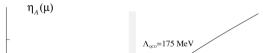
Figure 3: The value of $\eta_{A}(\mu)$ for $\Lambda_{\rm QCD}^{\overline{\rm MS}}=90\,\mbox{MeV}$, $130\,\mbox{MeV}$ and $175\,\mbox{MeV}$. The value of $\eta_{A}(\mu)$ must be used in the QCD-based calculations of the exclusive zero-recoil $B\rightarrow D^{*}$ form factor when nonperturbative effects are addressed. The shaded bars show the perturbative uncertainty irreducible without considering $1/m_{c}^{3}$ and $1/m_{c}^{4}$ effects; they give the lower bound for the corresponding actual nonperturbative corrections.

Conceptually, the deficiency of the alternative usage of the sum rules of Refs. [8, 17] chosen in [45] is to gauge $\xi_{A}$ on the value of $\eta_{A}^{2}$ as it has been defined in the HQET (the idea that $\xi_{A}$ is to be identified with $\eta_{A}^{2}$ ascends to [42, 41]): the value of $\eta_{A}$ is defined as an all-order ‘purely perturbative’ renormalization factor of the zero-recoil axial current. However, it is this factor $\eta_{A}$ that is ill-defined, and only for this reason must the difference between the stable Wilson coefficient $\xi_{A}$ and $\eta_{A}^{2}$ suffer from large corrections. It is worth reiterating once more in this respect that, in reality, $\eta_{A}$ cannot be equal to a matching coefficient of $\bar{c}\gamma_{\mu}\gamma_{5}b$ to a corresponding current in any effective field theory completely defined at the level of the nonperturbative physics.

The accurate analysis thus shows that the literal implementation of Wilson’s OPE not only eliminates purely theoretical problems with the IR renormalons, but also makes the actual impact of the higher-order perturbative corrections well-controlled.

4 Bounds on the transition formfactors from analyticity and unitarity

The kinematic point of zero recoil in the $b\rightarrow c$ semileptonic transitions is the least uncertain one for the theoretical analysis. On the other hand, experimentally the statistics is limited here. Therefore, information about the $q^{2}$-dependence of the formfactors is very important. However, is has a dynamical origin and is unknown a priori. Indeed, if the $B$ meson is relatively ‘soft’, i.e. the typical velocity of the effective light degrees of freedom is small – as would be the case in the nonrelativistic quark models – then the formfactor (the IW function) changes at the velocity transfer much less than unity, and this implies large derivatives ${\rm d}F(\vec{v}^{\,2})/{\rm d}\vec{v}^{\,2}$, ${\rm d}^{2}F(\vec{v}^{\,2})/({\rm d}\vec{v}^{\,2})^{2}$, etc. If, on the contrary, the bound state is relatively simple and the light degrees of freedom are ultrarelativistic, these derivatives are expected to be of order unity. Can something be stated about them without actual information about the bound state dynamics? I will argue below that the answer is negative.

An idea was put forward a few years ago to constraint the IW function using, mainly, general analyticity and unitarity properties of the formfactors in the heavy quark limit [51]. They turned out to be non-informative due to the presence of the $Q\bar{Q}$-bound states below the threshold of the open flavor production. This approach was resurrected recently in a number of publications [52, 53]. In particular, it was claimed in [53] to have established an intriguing relation between the slope and the curvature of the formfactor near the zero recoil kinematics. However, there are essential flaws in that analysis.

The general idea is to consider the transition formfactor for some $\bar{c}\,b$ current between $B$ and $D$ mesons as an analytic function of the momentum transfer $q^{2}$:

$$\langle D(p+q)|\>\bar{c}\,b\,(0)\>|B(p)\rangle\;=\;2\sqrt{M_{B}M_{D}}\;F_{S}(q^{2})$$ (37)

where, for simplicity, we can consider the scalar current not yielding irrelevant Lorentz indices.

The function $F_{S}$ in the physical $t$-channel domain $q^{2}\leq t_{\rm zr}=(M_{B}-M_{D})^{2}$ describes the decay amplitude and is real. On the other hand, analytically continued to large $q^{2}>(M_{B}+M_{D})^{2}$ it describes the exclusive production of $B\bar{D}$ in ${\rm e^{+}e^{-}}$-annihilation–type process and thus, in principle, is also an observable quantity. $F_{S}$ is complex there. Under the usual assumptions of analyticity one can write the dispersion integral for $F_{S}$:

$$F_{S}(q^{2})\;=\;\frac{1}{\pi}\,\int\;\frac{{\rm Im}\,F_{S}(t+i\epsilon)}{t-q^{2}-i\epsilon}\,dt\;=\;\frac{1}{\pi}\,\int_{t<(M_{B}+M_{D})^{2}}\;\frac{{\rm Im}\,F_{S}(t)}{t-q^{2}-i\epsilon}\,dt\;+$$

$$+\;\frac{1}{\pi}\,\int_{t>(M_{B}+M_{D})^{2}}\;\frac{{\rm Im}\,F_{S}(t)}{t-q^{2}-i\epsilon}\,dt\;\equiv\;F_{S}^{(r)}(t)\;+F_{S}^{(c)}(t)\;.$$ (38)

If the sub-threshold contribution from ${\rm Im}\,F_{S}(t)$ for $t<(M_{B}+M_{D})^{2}$ were small, the formfactor would be saturated by the second integral, $F_{S}\simeq F_{S}^{(c)}$. In that case the formfactor would be essentially constrained: since the exclusive production of $B\bar{D}$ must not yield the production cross section in this channel larger than the total hadronic one which is bound theoretically, $F$ cannot be too large in the wide domain. If one additionally has the normalization

$$F_{S}(t_{\rm zr})\;=\;1$$ (39)

(which holds at large $m_{b,c}$) then only little room would have been left and, for example, an almost functional relation between $F^{\prime}_{S}(t_{\rm zr})$ and $F^{\prime\prime}_{S}(t_{\rm zr})$ emerged [53].

This reasoning, however, crucially relies on the insignificance of the sub-threshold support of ${\rm Im}\,F(q^{2})$; on the other hand, it is generally known not to hold for heavy quarks. On the contrary, the common wisdom is that the first resonances dominate the formfactor. The idea of Ref. [53] was to consider the formfactor $F_{S}$ which does not have a contribution from the well-studied vector quarkonia. It was assumed that no clear-cut resonances below the $B\bar{D}$ threshold exist in the corresponding channel.

This basic assumption is erroneous, however. The sub-threshold scalar $0^{++}$ states are present both in the $\bar{c}c$ and $\bar{b}b$ systems ($\chi_{c,b}$ states) and, according to the general theorems, must be also in the $\bar{b}c$ channel. They are extremely narrow since lie below the open-flavor thresholds, and are expected to dominate the formfactor.

To account for the possible effect of the domain $q^{2}<(M_{B}+M_{D})^{2}$, Ref. [53] equated the whole sub-threshold contribution with the possible nonresonant one and considered a smooth model for ${\rm Im}\,F_{S}$ below the threshold:

$${\rm Im}\,F_{S}(t)\;\simeq\;\frac{M_{B}+M_{D}}{2\sqrt{M_{B}M_{D}}}\;\frac{C}{\sqrt{t_{0}}}\,\sqrt{t-(M_{B_{c}}+m_{\eta})^{2}}\;\;,\;\;\;\;(M_{B_{c}}+m_{\eta})^{2}<t<(M_{B}+M_{D})^{2}$$ (40)

with $C$ of order 1. As explained above, such a functional form is irrelevant below the threshold. Moreover, it is easy to calculate its contribution to the zero-recoil value $F_{S}((M_{B}\!-\!M_{D})^{2})\,$:

$$F_{S}^{(r)}(0)\;\simeq\;0.008\,C$$ (41)

(recall that in the usual pole-dominance models this value must be just close to unity). Thus, the effect of the states lying below the open flavor threshold was underestimated by two orders of magnitude.

The analysis of Ref. [53] applied to the scalar $\bar{c}\,b$ formfactor. Obtaining model-independent information about any formfactor would be very interesting by itself from the theoretical viewpoint. Phenomenologically, however, one needs to know the axial-vector formfactors, or those in the heavy quark limit $m_{Q}\rightarrow\infty$. In the heavy quark limit all these formfactors are related to the IW function; unfortunately, the $1/m_{c}$ corrections in the derivatives are too significant. Although they were claimed to be very mild, in reality it was based only on some perturbative estimates. On the other hand, the main, nonperturbative $1/m_{c}$ corrections are known to be large [54], $\sim 50\%$.

Can these problems be cured? One could have tried to consider similar dispersion relations at arbitrary masses $m_{c,b}$. Decreasing $m_{c}$ would soften the problem of the sub-threshold physics – however, the corrections in the short-distance expansions and to the necessary heavy quark symmetry relations are already marginal. Attempts to increase $m_{c}$ to tackle the $1/m_{c}$ corrections magnify the role of the sub-threshold behavior of the formfactor.

It is important that, contrary to the forward scattering amplitudes or current correlators, the phase of the formfactor has only an indirect physical meaning, and below the threshold is a very unphysical quantity not observable directly. For this reason its behavior in this domain can be rather odd and crucially depends on irrelevant details of the strong interactions which we know almost nothing about; by no means, for example, ${\rm Im}\,F$ must be positive for heavy quarks.

A very instructive analysis had been given a few years ago in the inspiring papers [55] which, unfortunately, are to a large extent forgotten in the recent literature. It was argued there that, just if the heavy flavor transition formfactor is governed by relatively soft clouds of light degrees of freedom, in the $s$-channel one should expect a complicated oscillating behavior of the production formfactor near the threshold; it can be simple if the transition formfactor is a slowly varying function (a ‘hard-core’ bound state) and then the lowest-pole dominance is expected to work.

One has to conclude, once again, that without actual dynamical input, the general analyticity and unitarity relations cannot per se yield useful information about the transition formfactors of interest. From the phenomenological perspective, the analysis [53] grossly underestimated both the sub-threshold contributions and the corrections [54] to the heavy quark symmetry constraints it relied on. The relation between the slope and the curvature claimed there rather should not be used in experimental analyses for deriving model-independent results.

The possibility to employ additional dynamical information, e.g. in the form of the lattice calculations of the formfactors at some intermediate points [56], must be explored in order to revive this approach.

5 The semileptonic branching ratio

In the QCD-based heavy quark expansion the total nonleptonic decay widths of heavy flavors can be treated in the same way as semileptonic or radiative ones; the difference appears only at a quantitative level. The statement about the absence of $1/m_{Q}$ corrections applies as well, and the leading corrections $\sim 1/m_{Q}^{2}$ have been calculated [6, 7, 12]. The overall semileptonic branching ratio ${\rm BR_{sl}}(B)$ seems to be of a particular practical interest: while the simple-minded parton estimates yield ${\rm BR_{sl}}(B)\simeq 15\%$ [57], experiment gives smaller values, ${\rm BR_{sl}}(B)\simeq 10.5$–$11.5\%$ (the current situation is reviewed by T. Browder).

The generic scale of the $1/m_{b}^{2}$ effects in the widths of individual nonleptonic channels is about $15\%$; however, the particular $V$–$A$ chiral and color structure of weak currents significantly suppresses it; moreover, an additional cancellation between different parton channels occurs, and one literally gets [58]

$$-\Delta_{1/m^{2}}\left({\rm BR_{sl}}\right)\;\mathrel{\hbox to0.0pt{\lower 3.0pt\hbox{\hskip 0.0pt$\sim$}\hss}\raise 1.0pt\hbox{$<$}}\;0.5\%\;\;.$$ (42)

Estimated $1/m_{b}^{3}$ corrections do not produce a significant effect either [59]. As a result, most of the attention was paid to a more accurate treatment of the perturbative corrections, in particular, accounting for the effect of the charm mass in the final state. It was found [60, 61] that the nonleptonic width is indeed boosted up.

Since the inclusive widths are expanded in inverse powers of energy release, one a priori expects larger corrections or even a breakdown of the expansion and violation of duality in the channel $b\rightarrow c\bar{c}s(d)$; however, this channel can be isolated [6] via charm counting, i.e. measuring the average number of charm quarks per beauty decay. The original experimental estimate $n_{c}\mathrel{\hbox to0.0pt{\lower 3.0pt\hbox{\hskip 0.0pt$\sim$}\hss}\raise 1.0pt\hbox{$<$}}1.15$ did not allow one to attribute the apparent discrepancy to this channel, and gave rise to the so-called ‘${\rm BR_{sl}}$ versus $n_{c}$’ problem.

The perturbative corrections in the $b\rightarrow c\bar{u}d$ itself cannot naturally drive $\rm BR_{sl}$ below $12.5\%$; the calculation for the $b\rightarrow c\bar{c}s(d)$ channel is less certain and, in principle, admits increasing the width by a factor of $1.5$ or even $2$, leading to $n_{c}\simeq 1.25$–$1.3$. In the latter case a value of $\rm BR_{sl}$ as low as $11.5\%$ can be accommodated.

The experimental situation with $n_{c}$ does not seem to be quite settled yet:

$$n_{c}=1.134\pm 0.043\qquad\mbox{(CLEO) }\;,\qquad\qquad n_{c}=1.23\pm 0.07\qquad\mbox{(ALEPH) }\;.$$

In a recent analysis [62] it was argued that consistency requires a major portion of the final states in the $b\rightarrow c\bar{c}s$ to appear as modes with the wrong-sign $D$’s and kaons but $D_{s}$, which previously escaped proper attention, and this allowed for a larger value $n_{c}\simeq 1.3$ needed to resolve the problem with $\rm BR_{sl}$. The dedicated theoretical consideration [63] shows that, indeed, the dominance of such modes is natural and this possibility does not require a significant violation of duality. Thus, if a larger value of $n_{c}\simeq 1.25$ is confirmed experimentally, the problem of $\rm BR_{sl}$ will not remain.

Even within this successful scenario a concern can be raised if a strong QCD-enhancement of a tree-level–unsuppressed decay mode, possibly achieved in the one-loop calculations, is trustworthy: one would need to boost the tree-level $b\rightarrow c\bar{c}s$ width by a factor of two. One should note, however, that theoretically the situation maybe not so pessimistic: the tree level estimate of ${\rm BR_{sl}}(b\rightarrow c\bar{c}s)\simeq 15\%$ [57] refers only to using the large values of the quark masses close to their pole values. Using the short-distance masses like $m_{b}\simeq 4.5\,\mbox{GeV}$ always yielded a larger starting value of the branching for this channel. Without addressing the strong interaction effects it must be viewed, conservatively, as an uncertainty of the simplest partonic predictions. However, it is more consistent, from the viewpoint of the OPE, to always use the values of the parameters entering at a particular level of computations; in the case of the $B$ widths it means that the smaller short-distance masses are preferable as the starting approximation. If one accepts this attitude, the actual corrections to the decay rate found at the one-loop level are rather mild and do not prompt immediate concerns about the theoretical control over the perturbative expansion. The observed large corrections to ${\rm BR_{sl}}(b\rightarrow c\bar{c}s)$ are then merely a response to an improper zeroth-order approximation.

6 Lifetimes of beauty particles

The QCD-based HQE provides a systematic framework for calculating the total widths of heavy flavors, which are not amenable to the traditional methods of HQET. The only assumption is that the mass of decaying quark (actually, the energy release) is sufficiently large; for a review, see [64].

A thoughtful application of this expansion to charm particles demonstrated that the actual expansion parameter appeared to be too low to ensure a trustworthy accurate description, so that a priori one expects only emergence of the qualitative features. Surprisingly, in many cases the expansion works well enough even numerically. In particular, it predicts $\tau_{D^{+}}\approx 2\tau_{D^{0}}$ as an effect of Pauli interference in $D^{+}$ and suggests $\tau_{D_{s}}\approx\tau_{D^{0}}$ – simultaneously correctly predicting the semileptonic fraction in $D$ mesons. A similar agreement seems to be observed in charm baryons (for a recent review, see [65]).

Applying the expansion to beauty particles one expects a decent numerical accuracy, although the overall scale of the preasymptotic effects is predicted to be small and makes a challenge to experiment:

$$\begin{array}[]{cclcl}\tau_{B^{-}}/\tau_{B^{0}}&\simeq&1+0.04\left(\frac{f_{B}}{180\,\rm MeV}\right)^{2}&\cite[cite]{[\@@bibref{}{mirage}{}{}]}&\qquad\mbox{ EXP: }\qquad 1.04\pm 0.04\\ \overline{\tau}_{B_{s}}/\tau_{B^{0}}&\simeq&1+{\cal O}(1\%)&\cite[cite]{[\@@bibref{}{mirage}{}{}]}&\qquad\mbox{ EXP: }\qquad 0.97\pm 0.05\\ (\tau_{B_{s}^{L}}-\tau_{B_{s}^{S}})/\tau_{B_{s}}&\simeq&0.18\left(\frac{f_{B_{s}}}{200\,\rm MeV}\right)^{2}&\cite[cite]{[\@@bibref{}{vsku}{}{}]}&\\ \tau_{\Lambda_{b}}/\tau_{B^{0}}&\approx&0.9&&\qquad\mbox{ EXP: }\qquad 0.78\pm 0.06\\ \end{array}$$ (43)

These differences appear mainly as $1/m_{b}^{3}$ corrections and, depending on certain four-fermion matrix elements, cannot be predicted at present very accurately. In particular, it refers to the preasymptotic effects in baryons. For mesons the estimates are based on the vacuum saturation approximation, which cannot be exact either. The impact of non-factorizable terms has been studied a few years ago in [67] and possibilities to directly measure the matrix elements in future experiments were suggested.

The apparent agreement with experiment is obscured by the reported lower values of $\tau_{\Lambda_{b}}$. Since the baryonic matrix elements are rather uncertain, quite a few model estimates have been done (see the recent one [68], and references therein). All seem to fall short; however, this might be attributed to deficiencies of the simple quark model. It was shown [69] using quite general arguments that, irrespective of the details, one cannot have an effect exceeding $10-12\%$ while residing in the domain of validity of the standard $1/m_{Q}$ expansion itself; the natural ‘maximal’ effects that can be accommodated are $\sim 7\%$ and $\sim 3\%$ for weak scattering and interference, respectively.

Thus, if the low experimental value of $\tau_{\Lambda_{b}}$ is confirmed, it will require a certain revision of the standard picture of the heavy hadrons and of convergence of the $1/m_{Q}$ expansion for nonleptonic widths.

7 $1/m_{Q}$ expansion and duality violation

The problem of duality violation attracts more and more attention of those who study the heavy quark theory; a recent extensive discussion was given in [70]. The expansion in $1/m_{Q}$ is asymptotic. There are basically two questions one can ask here: what is the onset of duality, i.e. when does the expansion start to work? The most straightforward approach was undertaken in Ref. [71], and no apparent indication toward an increased energy scale was found. Another question, how is the equality of the QCD parton-based predictions with the actual decay rates achieved, was barely addressed. Though a relevant example of such a problem is easy to give.

The OPE in full QCD ensures that no terms $\sim 1/m_{Q}$ can be in the widths and the corrections start with $1/m_{Q}^{2}$. However, the OPE per se cannot forbid a scenario where, for instance,

$$\frac{\delta\Gamma_{H_{Q}}}{\Gamma_{H_{Q}}}\;\sim\ \;C\;\frac{\sin{(m_{Q}\rho)}}{m_{Q}\rho}\;,\;\;\;\rho\sim\Lambda_{\rm QCD}^{-1}\;.$$ (44)

In the actual strong interaction, $m_{b}$ and $m_{c}$ are fixed and not free parameters, so, from the practical viewpoint these types of corrections are not too different – but the difference is profound in the theoretical description! It reflects specifics of the OPE in Minkowski space, and such effects can hardly be addressed, for example, in the lattice simulations. Their control requires a deeper understanding of the underlying QCD dynamics beyond the knowledge of first few nonperturbative condensates.

In fact, the literal corrections of the type of eq. (44) are hardly possible; the power of $1/m_{Q}$ in realistic scenarios is larger, and these duality corrections must be eventually exponentially suppressed though, probably, starting at a higher scale [70]. But a theory of such effects is still in its embryonic stage and needs an additional experimental input as well.

8 Conclusions

I would like to conclude this admittedly incomplete review of the theory and applications of the heavy quark expansion by the following general remark. It was sometimes said already a few years ago that the theory of heavy quark decays was basically completed and only a few technical refinements remained to be done. The subsequent development clearly showed that the potential for further studies was vast. Regarding the current status, I believe that, although the basic principles of the HQE in QCD are formulated and well studied, we still have many interesting things to understand and calculate even in the original, the most standard fields of applications – before one can actually consider the theory completed.

Acknowledgements:   I am grateful to the organizers of CRAD ‘96 for the opportunity to participate in this Symposium. The financial support and hospitality of the CERN Theory Division are gratefully acknowledged. The collaboration with I. Bigi, M. Shifman and A. Vainshtein was highly beneficial; I am also thankful to M. Voloshin for many clarifications. This work was supported in part by NSF under the grant number PHY 92-13313.

References

-
[1]
K. Wilson, Phys. Rev. 179 (1969) 1499;
K. Wilson and J. Kogut, Phys. Rep. 12 (1974) 75. -
[2]
W.E. Caswell and G.P. Lepage, Phys. Lett. B 167
(1986) 437;
G.P. Lepage, L. Magnea, C. Nakleh, U. Magnea, and K. Hornbostel, Phys. Rev. D46 (1192) 4052. - [3] S. Balk, J.G. Körner and D. Pirjol, Nucl. Phys. B428 (1994) 499.
- [4] H. Georgi, Phys. Lett. B 240 (1990) 447.
- [5] V. Novikov, M. Shifman, A. Vainshtein and V. Zakharov, Nucl. Phys. B249 (1985) 445.
- [6] I. Bigi, N.G. Uraltsev and A. Vainshtein, Phys. Lett. B 293 (1992) 430.
- [7] B. Blok and M. Shifman, Nucl. Phys. B399 (1993) 441 and 459.
- [8] M. Shifman, N.G. Uraltsev and A. Vainshtein, Phys. Rev. D51 (1995) 2217.
- [9] M. Voloshin, Surv. High En. Phys. 8 (1995) 27.
- [10] P. Ball and V. Braun, Phys. Rev. D49 (1994) 2472; for an update, see E. Bagan, P. Ball, V. Braun and P. Gosdzinsky, Phys. Lett. B342 (1995) 362.
- [11] I. Bigi, A. Grozin, M. Shifman, N.G. Uraltsev and A. Vainshtein, Phys. Lett. B339 (1994) 160.
- [12] I. Bigi, B. Blok, M. Shifman, N.G. Uraltsev and A. Vainshtein, The Fermilab Meeting, Proc. of the 1992 DPF meeting of APS, C.H. Albright et al. (World Scientific, Singapore 1993), vol. 1, p. 610.
- [13] I. Bigi, M. Shifman, N.G. Uraltsev and A. Vainshtein, Phys. Rev. Lett. 71 (1993) 496.
- [14] M. Voloshin, Phys. Rev. D51 (1995) 4934.
- [15] N.G. Uraltsev, Int. J. Mod. Phys. A11 (1996) 515.
- [16] I. Bigi and N.G. Uraltsev, Phys. Lett. B 321 (1994) 412.
- [17] I. Bigi, M. Shifman, N.G. Uraltsev and A. Vainshtein, Phys. Rev. D52 (1995) 196.
- [18] D. Dikeman, M. Shifman and N.G. Uraltsev, Int. J. Mod. Phys. A11 (1996) 571.
- [19] I. Bigi, M. Shifman, N.G. Uraltsev and A. Vainshtein, Phys. Rev. D50 (1994) 2234.
- [20] M. Beneke and V. Braun, Nucl. Phys. B426 (1994) 301.
- [21] M. Gremm, A. Kapustin, Z. Ligeti and M.B. Wise, Phys. Rev. Lett. 77 (1996) 20.
- [22] M. Beneke, V.M. Braun and V.I. Zakharov, Phys. Rev. Lett. 73 (1994) 3058.
- [23] M.B. Voloshin, Int. J. Mod. Phys. A10 (1995) 2865.
- [24] M. Luke, M. Savage and M. Wise, Phys. Lett. B343 (1995) 329; B345 (1995) 301.
- [25] P. Ball, M. Beneke and V. Braun, Phys. Rev. D52 (1995) 3929.
- [26] M. Neubert, Preprint CERN-TH/95-107 [hep-ph/9505238] (Proc. of the th Rencontres de Moriond, Les Arcs, France, March 1995).
- [27] I am grateful to M. Voloshin for the discussion of these numerical aspects.
- [28] R.E. Behrends et al., Phys. Rev. 101 (1956) 866.
- [29] A. Czarnecki, Phys. Rev. Lett. 76 (1996) 4124.
- [30] I. Bigi, M. Shifman, N.G. Uraltsev and A. Vainshtein, Preprint CERN-TH/96-191.
- [31] P. Ball and U. Nierste, Phys. Rev. D50 (1994) 5841.
- [32] ALEPH collaboration, PA05-059 “Inclusive Measurement of Charmless Semileptonic Branching Ratio of -Hadrons”, contribution to the XXVIII International Conference on High Energy Physics, Warsaw, Poland 25-31 July 1996.
- [33] M. Neubert, Preprint CERN-TH/95-307 [hep-ph/9511409] (unpublished), and later preprints.
-
[34]
M. Voloshin and M. Shifman, Yad. Fiz. 47 (1988) 801
[Sov. J. Nucl. Phys. 47 (1988) 511];
M.A. Shifman, in: Proceedings of the Int. Symposium on Production and Decay of Heavy Hadrons, Heidelberg (1986). - [35] M.E. Luke, Phys. Lett. B252 (1990) 447.
- [36] M. Neubert, Phys. Rep. 245 (1994) 259.
- [37] M. Neubert, Preprint CERN-TH. 7225/94, April 1994 [hep-ph/9404296].
- [38] N.G. Uraltsev, Mod. Phys. Lett. A10 (1995) 1803.
- [39] M. Neubert, Phys. Rev. D46 (1992) 2212.
- [40] M. Neubert, Phys. Rev. D51 (1992) 5924.
- [41] M. Neubert, Phys. Lett. B338 (1994) 84.
- [42] M. Neubert and C.T. Sachrajda, Nucl. Phys. B438 (1995) 235.
- [43] N.G. Uraltsev, Preprint CERN-TH/96-304 [hep-ph/9610425].
- [44] J.G. Körner and D. Pirjol, Phys. Lett. B334 (1994) 399.
- [45] A. Kapustin, Z. Ligeti, M.B. Wise and B. Grinstein, Phys. Lett. B375 (1996) 327.
-
[46]
G. ’t Hooft, in The Whys Of Subnuclear Physics, Erice
1977, ed. A. Zichichi (Plenum, New York, 1977);
B. Lautrup, Phys. Lett. 69B (1977) 109;
G. Parisi, Phys. Lett. 76B (1978) 65; Nucl. Phys.
B150 (1979) 163;
A. Mueller, Nucl. Phys. B250 (1985) 327.
For a recent review see
A. H. Mueller, in Proc. Int. Conf. “QCD – 20 Years Later”, Aachen 1992, eds. P. Zerwas and H. Kastrup, (World Scientific, Singapore, 1993), vol. 1, page 162. - [47] Yu.L. Dokshitzer and N.G. Uraltsev, Phys. Lett. B380 (1996) 141.
- [48] G. Grunberg, Phys. Lett. B372 (1996) 121.
- [49] M. Luke, A. Manohar and M. Savage, Phys. Rev. D51 (1995) 4924.
- [50] J. G. Körner, K. Melnikov and O. Yakovlev, Zeit. f. Phys. C69 (1996) 437.
- [51] E. de Rafael and J. Taron, Phys. Lett. B282 (1992) 215; Phys. Rev. D50 (1994) 373.
- [52] C.G. Boyd, B. Grinstein and R.F. Lebed, Phys. Lett. B353 (1995) 306; Nucl. Phys. B461 (1996) 461.
- [53] I. Caprini and M. Neubert, Phys. Lett. B380 (1996) 376.
- [54] A. Vainshtein, Preprint TPI-MINN-95/34-T [hep-ph/9512419], Proc. EPS Conference on High Energy Physics, Brussels, July 1995.
-
[55]
R.L. Jaffe, Phys. Lett. B 245 (1990) 221;
R.L. Jaffe and P.F. Mende, Nucl. Phys. B369 (1992) 189. - [56] L.P. Lellouch, Nucl. Phys. B479 (1996) 353.
- [57] For a review, see G. Altarelli and S. Petrarca, Phys. Lett. B261 (1991) 303.
- [58] I. Bigi, B. Blok, M. Shifman and A. Vainshtein, Phys. Lett. B323 (1994) 408.
- [59] I. Bigi and N.G. Uraltsev, Phys. Lett. B 280 (1992) 271.
-
[60]
E. Bagan, P. Ball, V. Braun and P. Gosdzinsky,
Phys. Lett. B342 (1995) 362; (E) B374 (1996) 363;
E. Bagan, P. Ball, B. Fiol and P. Gosdzinsky, Phys. Lett. B351 (1995) 546. - [61] M. B. Voloshin, Phys. Rev. D51 (1995) 3948.
- [62] I. Dunietz, Preprint FERMILAB-PUB-96/104-T [hep-ph/9606247].
- [63] B.Blok, M. Shifman and N.G. Uraltsev, Preprint CERN-TH/96-252 [hep-ph/9610515].
- [64] I.I. Bigi, B.Blok, M. Shifman, N.G. Uraltsev and A. Vainshtein, in: B Decays, S. Stone (ed.), second edition (World Scientific, Singapore 1994), p. 132.
- [65] G. Bellini, I. Bigi and P.J. Dornan, Preprint UND-HEP-96-BIG02, to appear in Phys. Rep.
- [66] V.A. Khoze, M.A. Shifman, N.G. Uraltsev and M.B. Voloshin, Sov. J. Nucl. Phys. 46 (1987) 112 [Yad. Phys., 46 (1987) 181].
-
[67]
I. Bigi and N.G. Uraltsev, Nucl. Phys. B423 (1994) 33;
Zeit. f. Phys. C62 (1994) 623. - [68] J. Rosner, Phys. Lett. B379 (1996) 267.
- [69] N.G. Uraltsev, Phys. Lett. B376 (1996) 303.
- [70] B. Chibisov, R. Dikeman, M. Shifman and N.G. Uraltsev, Preprint CERN-TH/96-113 [hep-ph/9605465], to appear in IJMPA.
- [71] B. Blok and T. Mannel, Mod. Phys. Lett. A11 (1996) 1263.