Abstract

We give a review of modern theoretical understanding of the physics of $QCD$ at finite temperature. Three temperature regions are studied in details. When the temperature is low, the system presents a rarefied pion gas. Its thermodynamic and kinetic properties are adequately described by chiral perturbation theory.

When the temperature is increased, other than pion degrees of freedom are excited, the interaction between the particles in the heat bath becomes strong, and the chiral theory is not applicable anymore. At some point $T=T_{c}$ a phase transition is believed to occur. The physics of the transitional region is discussed in details. The dynamics and the very existence of this phase transition strongly depends on the nature of the gauge group, the number of light quark flavors, and on the value of quark masses. If the quarks are very heavy, the order parameter associated with the phase transition is the correlator of Polyakov loops $<P^{*}({\bf x})P(0)>_{T}$ related to the static potential between heavy colored sources. When the quark masses are small, the proper order parameter is the quark condensate $<\bar{q}q>_{T}$ and the phase transition is associated with the restoration of the chiral symmetry. Its dynamics is best understood in the framework of the instanton liquid model. Theoretical estimates and some numerical lattice measurements indicate that the phase transition probably does not occur for the experimentally observed values of quark masses . We have instead a very sharp crossover, ”almost” a second order phase transition.

At high temperatures $T\gg\mu_{hadr}$ the system is adequately described in terms of quark and gluon degrees of freedom and presents the quark–gluon plasma ($QGP$). Static and kinetic properties of $QGP$ are discussed. A particular attention is payed to the problem of physical observability, i.e. the physical meaningfulness of various characteristics of $QGP$ discussed in the literature.

CONTENTS

1. INTRODUCTION. 3

2. FINITE $T$ DIAGRAM TECHNIQUE. 8

2.1 Euclidean (Matsubara) technique. 8

2.2 Real time (Keldysh) technique. 9

3. PURE YANG–MILLS THEORY: DECONFINEMENT PHASE TRANSITION 19

3.1 Preliminary remarks. 19

3.2 Bubble confusion. 21

3.3 More on phase transition. 26

4. LUKEWARM PION GAS. 31

4.1 Chiral symmetry and its breaking 31

4.2 Thermodynamics 38

4.3 Pion collective excitations 39

4.4 Nucleons 48

4.5 Vector mesons. Experiment 53

5. CHIRAL SYMMETRY RESTORATION 55

5.1 General considerations.
Order of phase transition and critical behavior 55

5.2 Insights from soft pion physics. Large $N_{c}$ 60

5.3 The real world 66

5.4 Instantons and percolation 70

5.5 Disoriented chiral condensate 75

6. QUARK–GLUON PLASMA 76

6.1 Static properties of $QGP$: a bird eye’s view 77

6.2 Static properties of $QGP$: perturbative corrections 83

6.3 Collective excitations 90

6.4 Damping mayhem and transport paradise 97

6.5 Chirality drift 105

7. AKNOWLEDGEMENTS 116

REFERENCES 116

1 Introduction.

The properties of $QCD$ medium at finite temperature have been the subject of intense study during the last 15–20 years. It was realized that the properties of the medium undergo a drastic change as the temperature increases. At low temperatures, the system presents a gas of colorless hadron states: the eigenstates of the $QCD$ hamiltonian at zero temperature. When the temperature is small, this gas is composed mainly of pions — other mesons and baryons have higher mass and their admixture in the medium is exponentially small $\sim\exp\{-M/T\}$. At small temperature, also the pion density is small — the gas is rarefied and pions practically do not interact with each other.

However, when the temperature increases, pion density grows, the interaction becomes strong, and also other strongly interacting hadrons appear in the medium. For temperatures of order $T\sim$ 150 Mev and higher, the interaction is so strong that the hadron states do not present a convenient basis to describes the properties of the medium anymore, and no analytic calculation is possible.

On the other hand, when the temperature is very high, much higher than the characteristic hadron scale $\mu_{hadr}\sim$ 0.5 Gev, theoretical analysis becomes possible again. Only in this range, the proper basis are not hadron states but quarks and gluons — the elementary fields entering the $QCD$ lagrangian. One can say that, at high temperatures, hadrons get ”ionized” to their basic compounds. In the $0^{\underline{th}}$ approximation, the system presents the heat bath of freely propagating colored particles. For sure, quarks and gluons interact with each other, but at high temperatures the effective coupling constant is small $\alpha_{s}(T)\ll 1$ and the effects due to interaction can be taken into account perturbatively . This interaction has the long–distance Coulomb nature, and the properties of the system are in many respects very similar to the properties of the usual non-relativistic plasma involving charged particles with weak Coulomb interaction. The only difference is that quarks and gluons carry not the electric, but color charge. Hence the name: Quark-Gluon Plasma ($QGP$).

Thus the properties of the system at low and at high temperatures have nothing in common. A natural question arises: What is the nature of the transition from low-temperature hadron gas to high- temperature quark-gluon plasma ? Is it a phase transition ? If yes, what is its order ? I want to emphasize that this question is highly non-trivial. A drastic change in the properties of the system in a certain temperature range does not guarantee the presence of the phase transition point where free energy of the system or its specific heat is discontinuous. Recall that there is no phase transition between ordinary gas and ordinary plasma.

Whether or not the phase transition occurs in the real $QCD$ with particular values of quark masses is the question under discussion now. Our personal feeling is that the answer is probably negative and what really happens is not the phase transition but a sharp crossover — ”almost” a second-order phase transition. Another discussed possibility is that a weak first order phase transition (with small latent heat) still occurs. A point of consensus now is that the real phase transition does occur in some relative theories — in pure Yang- Mills theory (when the quark masses are sent to infinity) and in $QCD$ with 2 or 3 exactly massless quark flavors.

There are at least 4 reasons why this question is interesting to study:

1. It is just an amusing theoretical question.

2. Theoretic conclusions can be checked in lattice numerical experiments. Scores of papers devoted to lattice study of thermal properties of QCD have been published.

3. Perhaps, a direct experimental study would be possible on RHIC — high-energy ion collider which is now under construction.

4. During the first second of its evolution, our Universe passed through the stage of high-$T$ quark-gluon plasma which later cooled down to hadron gas (and eventually to dust and stars, of course). It is essential to understand whether the phase transition did occur at that time. A strong first-order phase transition would lead to observable effects. In particular, it could have created inhomogeneities in baryon number density in early Universe which would later affected nucleosynthesis and therefore leave a signature in the primordial nuclear abundances [1]. We know (or almost know — the discussion of this question has not yet completely died away) that there were no such transition. But it is important to understand why.

Note that there is also a related but different question — what are the properties of relatively cold but very dense matter and whether there is a phase transition when the chemical potential corresponding to the baryon charge rather than the temperature is increased. This review will be devoted exclusively to the thermal properties of QCD, and we shall assume zero baryon charge density.

At present, we are able to describe the physics of thermal phase transition mainly in qualitative terms (we will address, however, the issue of critical exponents and the critical amplitudes where certain theoretical predictions can be made). As was already mentioned, there are, however, two regions where many quantitative theoretical results can be obtained. These are the small temperature region where the system presents a weakly interacting rarefied pion gas and the high temperature region where the system presents a weakly interacting (and also rarefied in some sense) quark–gluon plasma.

In both cases, we are facing a reasonably clean and rather interesting problem of theoretical physics lying on cross-roads between the relativistic field theory and condensed matter physics. Personally, I had a great fun studying it. Unfortunately, at present only a theoretical study of the problem is possible. That concerns especially the high temperature phase. Hot hadron medium with the temperature above phase transition can be produced for tiny fractions of a moment in heavy ion collisions but:

• It is not clear at all whether a real thermal equilibrium is achieved.

• A hot system created in the collision of heavy nuclei rapidly expands and cools down emitting pions and other particles. It is not possible to probe the properties of the system directly, but only indirectly via the characteristics of the final hadron state.

• Anyway, the temperature achieved at existing accelerators is not high enough for the perturbation theory to work and there are no quantitative theoretical predictions with which experimental data can be compared. RHIC would be somewhat better in this respect, but even there the maximal temperature one could expect to reach is of order 0.5 GeV [3]. This is above the expected phase transition temperature $\sim 200$ MeV (see a detailed discussion in Chapters 4 and 5), but is still probably not high enough for the effective coupling constant to be small so that perturbative calculations would be justified.

Thus at present, there are no experimental tests of non-trivial theoretical predictions for $QGP$ properties. The effects observed in experiment such as the famous $J/\psi$ – suppression (for a recent review see [2]) just indicate that a hot and dense medium is created but says little on whether it is $QGP$ or something else.

The absence of proper feedback between theory and experiment is a sad and unfortunate reality of our time: generally, what is interesting theoretically is not possible to measure and what is possible to measure is not interesting theoretically .

The situation is somewhat better with numerical lattice experiments. One of the advantages of the lattice approach is that the question of whether thermal equilibrium is achieved does not arise — path integrals on an Euclidean cylinder with imaginary time size $\beta=1/T$ describe the partition function and other characteristics of the equilibrated system just by definition. A lot of numerical results at the temperatures below or slightly above critical temperature exist and in some cases they provide very useful insights which help to understand better the physics of the phase transition. In principle, one can also measure on the lattice the characteristics of the high temperature phase. Due to a finite size of the lattice, it is more difficult, however, and such studies just started. A limitation here is that we can calculate numerically only Euclidean path integrals which means that we can study only static characteristics of the system. Kinetic properties (spectrum of collective excitations in $QCD$ heat bath, the transport phenomena such as viscosity and electric conductivity, etc) cannot be probed in this way. (May be, it is possible, however, to study a nontrivial kinetic characteristics, the rate of axial charge non-conservation in high temperature phase, studying numerically classical Yang–Mills theory on a hamiltonian lattice. We will address this question at the end of the review.)

Thus we will not attempt (or almost will not attempt) to establish relation of the results of theoretical calculations with realistic accelerator experiments. Comparison with the lattice data will be done when the latter are available, i.e. in the low and moderate temperature region. What we will do, however, is discussing the relation of theoretical results with gedanken experiments. Suppose, we have a thermos bottle with hot hadron matter or with $QGP$ on a laboratory table and are studying it from any possible experimental angle. We call a quantity physical if it can in principle be measured in such a study and non-physical otherwise. We shall see later that many quantities discussed by theorists may be called physical only with serious reservations, and some are not physical at all.

Many reviews on the subject have already been written (see e.g. [2], [4] – [11]). However, all of them were either written a considerable time ago and do not cover very important recent developments or have a limited scope. I will try here to fill up this gap and present a modern discussion which covers a reasonably broad set of questions. Of course, I could not cover everything. The issues which interested me more and which I am more familiar with are discussed at greater length and in greater details. In cases when the question is still controversial and no general consensus exists, I will present my own viewpoint. A bias of this kind is, however, inevitable.

I had some problems in arranging the material and found no way not to break the causality: cross–references both back in text and forward in text will be abundant. The physics of all finite temperature systems has something in common, and the parallels will be drawn all the time. Moreover, some basic facts about quark–gluon plasma (the subject of Chapter 6) will be used in Chapter 3 where the physics of pure glue systems is discussed, etc.

But, anyway, some plan should be chosen, and it is the following. The next chapter presents technical preliminaries. I will give a review of finite $T$ diagram technique. A particular emphasis is given to the real time formalism which is most convenient when studying kinetic properties of the system. It is much less known than Euclidean Matsubara technique (well suited to study static characteristics) and has entered the standard tool kit of field thenrists studying thermal field theories only recently.

Chapter 3 is devoted to physics of pure Yang–Mills theory at finite $T$. The system displays deconfinement phase transition in temperature associated with changing the behavior of the potential between static quark sources. In particular, we discuss the structure of the high temperature phase and show that there is only one such phase, not $N_{c}$ different phases with domain walls between them as people believed for a long time and some continue to believe up to now. There is no such physical phenomenon as spontaneous breaking of $Z_{N}$ symmetry at high temperature in the pure Yang–Mills system.

In Chapter 4 we go over to the theories involving light dynamical quarks and discuss first the properties of low temperature phase. We discuss at length the temperature dependence of chiral condensate (it decreases with temperature) and also explore the fate of pions and massive hadron states at small nonzero temperature. We show that the leading effect of the pion heat bath on massive hadrons is that the latter acquire finite width. Real part of the poles of corresponding Green functions is also somewhat shifted. For nucleons, this shift is rather tiny. For vector mesons, the shift is also tiny in the temperature region up to $\sim 100$ MeV. What happens at higher temperatures is not quite clear by now and is a subject of intense discussions.

Chapter 5 is devoted to the physics of thermal phase transition in $QCD$. It is associated with restoration of chiral symmetry which is broken spontaneously at zero temperature. We show how the physics of the phase transition depends on the number of light quark flavors (For two massless flavors it is the second order while for three flavors it is the first order. We argue in particular that, in the theory with 4 or may be 5 massless flavors, chiral symmetry would probably not broken at all and, correspondingly, there would be no phase transition ). We discuss in details the physical mechanism of the phase transition which, in our opinion, is best understood in the framework of the instanton-antiinstanton liquid model. In this model, characteristic vacuum fields contributing in the Euclidean functional integral for the partition function present a collections of quasi-classical objects: instantons and antiinstantons. Each (anti)instanton supports fermion zero modes (one fermion and one antifermion zero mode for each flavor). When interaction between quasi-particles is taken into account, the modes shift from zero, but, as the interaction turns out to be strong enough, the characteristic eigenfunctions become delocalized and characteristic distance between neighboring eigenvalues is very small $\sim 1/V^{Eucl}$. This brings about nonzero fermion condensate. When temperature is increased, the density of quasi- particles decreases and, which is even more important, their interaction decreases. As a result, instantons and antiinstantons tend to form ”molecules” with localized fermion eigenfunctions. Characteristic eigenvalues are far from zero in this case and the chiral condensate is zero. Remarkably, it is basically the same mechanism which brings about the so called ”percolation phase transition in doped semiconductors”. When the density of impurity is high, electrons can jump between adjacent impurity atoms, acquire mobility, and the material becomes a conductor. In the end of the chapter we discuss the phenomenon of disoriented chiral condensate.

Physics of $QGP$ is discussed in Chapter 6. We discuss the limits of applicability of perturbation theory due to so called ”magnetic screening” - the effect which is specific for nonabelian gauge theories. We discuss also the spectrum of plasmons and plasminos — the collective excitations with quantum numbers of quarks and gluons in $QGP$. We address the controversial issue of the plasmon damping. We show that damping depends on the gauge convention and has as such little physical meaning. On the contrary, transport phenomena (such as viscosity, electric conductivity, energy losses of a heavy energetic particle passing through $QGP$, etc.) are quite physical and can be measured in a gedanken experiment. Finally, we discuss a pure non-perturbative effect of chirality non-conservation in quark-gluon plasma (or, if you will baryon number non-conservation in hot electroweak plasma). The rate of non-conservation is proportional to $T^{4}$ times a power of coupling constant. What is this power and whether a numerical algorithm exists where this quantity can be determined is still a question under discussion now.

2 Finite $T$ diagram technique.

The main point of interest for us are the physical phenomena in hot QCD system. However, as the main theoretical tool to study them is the perturbation theory and we want in some cases not only to quote the results, but also to explain how they are obtained, we are in a position to spell out how the perturbative calculations at finite $T$ are performed.

There are two ways of doing this — in imaginary or in real time. These techniques are completely equivalent and which one to use is mainly a matter of taste. Generally, however, the Euclidean technique is more handy when one is interested in pure static properties of the system (thermodynamic properties and static correlators) where no real time dependence is involved. On the other hand, when one is interested in kinetic properties (spectrum of collective excitations, transport phenomena, etc.), it is much more convenient to calculate directly in real time.

2.1 Euclidean (Matsubara) technique.

Many good reviews of Matsubara technique are available in the literature (see e.g. [9]) and we will describe it here only briefly. Consider a theory of real scalar field described by the hamiltonian $H[\phi({\bf x}),\ \Pi({\bf x})]$. The partition function of this theory at temperature $T$ can be written as

$$Z={\rm Tr}\left\{e^{-\beta H}\right\}=\int\prod_{\bf x}d\phi({\bf x}){\cal K}[\phi({\bf x}),\phi({\bf x});\beta]$$ (2.1)

where ${\cal K}$ is the quantum evolution operator in the imaginary time $\beta=1/T$ :

$${\cal K}[\phi^{\prime}({\bf x}),\phi({\bf x});\beta]=\sum_{n}\Psi_{n}^{*}[\phi^{\prime}({\bf x})]\Psi_{n}[\phi({\bf x})]e^{-\beta E_{n}}$$ (2.2)

$\Psi_{n}$ are the eigenstates of the hamiltonian. One can express the integral in RHS of Eq.(2.1) as an Euclidean path integral:

$$Z=\int\prod_{{\bf x},\tau}d\phi({\bf x},\tau)\exp\left\{-\int_{0}^{\beta}d\tau\int d{\bf x}\ {\cal L}[\phi({\bf x},\tau]\right\}$$ (2.3)

where the periodic boundary conditions are imposed

$$\phi({\bf x},\tau+\beta)=\phi({\bf x},\tau)$$ (2.4)

A thermal average $<{\cal O}>_{T}$ of any operator ${\cal O}[\phi({\bf x},\tau)]$ has the form [12]

$$<{\cal O}>_{T}=Z^{-1}\int\prod_{{\bf x},\tau}d\phi({\bf x},\tau){\cal O}[\phi({\bf x},\tau)]\exp\left\{-\int_{0}^{\beta}d\tau\int d{\bf x}\ {\cal L}[\phi({\bf x},\tau]\right\}$$ (2.5)

One can develop now the diagram technique in a usual way. The only difference with the zero temperature case is that the Euclidean frequencies of the field $\phi({\bf x},\tau)$ are now quantized due to periodic boundary conditions (2.4):

$$p_{0}^{n}=2\pi inT$$ (2.6)

with integer $n$. To calculate something, one should draw the same graphs as at zero temperature and go over into Euclidean space where the integrals over Euclidean frequencies are substituted by sums:

$$\int\frac{d^{4}p}{(2\pi)^{4}}f(p)\longrightarrow T\sum_{n}\int\frac{d^{3}p}{(2\pi)^{3}}f(2\pi inT,{\bf p})$$ (2.7)

The same recipe holds in any theory involving bosonic fields. In theories with fermions, one should impose antiperiodic boundary conditions on the fermion fields $\psi({\bf x},\tau)$ (see e.g. [13] for detailed pedagogical explanations), and the frequencies are quantized to

$$p_{0}^{n}=i\pi(2n+1)T$$ (2.8)

An important heuristic remark is that, when the temperature is very high, in many cases only the bosons with zero Matsubara frequencies $p_{0}=0$ contribute in $<{\cal O}>_{T}$. The contribution of higher Matsubara frequencies and also the contribution of fermions in $<{\cal O}>_{T}$ become irrelevant and, effectively, we are dealing with a 3- dimensional theory. As was just mentioned, it is true in many, but not in all cases. For example, it makes no sense to neglect fermion fields when one is interested in the properties of collective excitations with fermion quantum numbers. For any particular problem of interest a special study is required.

2.2 Real time (Keldysh) technique.

Matsubara technique is well suited to find thermal averages of static operators ${\cal O}({\bf x})$. If we are interested in a time-dependent quantity, there are two options: i) To find first the thermal average $<{\cal O}({\bf x},\tau)>$ for Euclidean $\tau$ and perform then an analytic continuation onto the real time axis. It is possible, but quite often rather cumbersome. ii) To work in the real time right from the beginning. The corresponding technique was first developed in little known papers [14] and independently by Keldysh [15] who applied it to condensed matter problems with a particular emphasis on the systems out of equilibrium. For systems at thermal equilibrium, it was effectively reinvented in a slightly different approach in the seventies by the name “thermo field dynamics” [16]. It was fully apprehended by experts in relativistic field theory only in the beginning of the nineties.

There is no good review on real time diagram technique addressed to field theorists. The existing review [17] is very deep and extensive, but is written rather formally and is hard to read. What we will do here is in a sense complementary to the review [17]. We will not derive the real time technique in a quite accurate and regular way, but rather elucidate its physical foundations, show how multicomponent Green’s functions appear, formulate and discuss the real time Feynman rules, and discuss also a simplistic but rather useful version of the real time technique due to Dolan and Jackiw [18].

Consider a quantum mechanical system in thermal equilibrium. Suppose a thermal average (2.5) of a Heisenberg operator ${A}_{0}(t)$ is zero. Let us perturb the system adding to the hamiltonian the term

$$V(t)\ =\ V_{0}\hat{B}_{0}\delta(t)$$ (2.9)

where $B_{0}$ is some operator and we assume the constant $V_{0}$ to be small. The Heisenberg operator $A_{H}(t)$ of the full hamiltonian $H\ =\ H_{0}+V(t)$ is related to the Heisenberg operator ${A}_{0}(t)$ of unperturbed hamiltonian (or the operator in interaction representation) as

$$A_{H}(t)\ =\ \exp\left\{i\int_{-\infty}^{t}V(\tau)d\tau\right\}A_{0}(t)\exp\left\{-i\int_{-\infty}^{t}V(\tau)d\tau\right\}$$ (2.10)

(Generally, $T$–ordered exponentials enter, but for an instantaneous perturbation $T$–ordering is irrelevant). In the first order in $V_{0}$

$$A_{H}(t)\ =\ A_{0}(t)-iV_{0}\theta(t)\left[A_{0}(t),B_{0}\right]$$ (2.11)

The thermal average is

$$<A_{H}(t)>_{T}\ =\ -iV_{0}<\theta(t)[A_{0}(t),B_{0}]>_{T}$$ (2.12)

The expression in the RHS of Eq. (2.12) is called the response function — it determines the response of the system at some time $t>0$ at the instantaneous small perturbation applied at $t=0$. Let us make a Fourier transform and define the generalized susceptibility

$$D^{AB}(\omega)\ =\ -i\int_{-\infty}^{\infty}e^{i\omega t}\theta(t)<\left[A_{0}(t),B_{0}\right]>_{T}dt$$

$$=\ \sum_{nm}e^{-E_{n}/T}\left[\frac{A_{nm}B_{mn}}{\omega+E_{n}-E_{m}+i0}-\frac{B_{nm}A_{mn}}{\omega+E_{m}-E_{n}+i0}\right]$$ (2.13)

We see that $D^{AB}(\omega)$ is analytic in the upper half–plane. It is just the corollary of the fact that $D^{AB}(t<0)\ =\ 0$. The relation (2.2) is well known in statistical mechanics and is called the Kubo formula.

Consider now a thermal field theory. Let it be first a theory of real scalar field with possible nonlinear interactions. Suppose the perturbation is coupled to $\phi({\bf x},0)$ and we measure the response of the system at some later time $t$ in terms of $<\phi({\bf x},t)>_{T}$. The corresponding response function is called the retarded Green’s function

$$D_{R}(t,{\bf x})\ =\ -i\theta(t)<[\phi(t,{\bf x}),\phi(0)]>_{T}$$ (2.14)

Its Fourier image $D_{R}(\omega,{\bf p})$ is analytic in the upper $\omega$ half-plane. One can show that the retarded Green’s function describes a natural analytic continuation of the Matsubara Green’s function (defined at a discrete set of points on the imaginary $\omega$ axis) on the complex $\omega$ plane. We will be mainly interested with real $\omega$.

On the tree level

$$D^{0}_{R}(\omega,{\bf p})\ =\ \frac{1}{(\omega+i0)^{2}-{\bf p}^{2}-m^{2}}$$ (2.15)

Let us separate now the free hamiltonian from the interaction part and build up the perturbation theory for $D_{R}(t,{\bf x})$ and other physically observable quantities in interaction representation. It is very well known that at zero temperature the retarded propagators like (2.15) are not quite convenient for this purpose. The matter is that to calculate, say, the exact retarded Green’s function, we have to draw the loops involving virtual particles which do not necessarily go forward in time. In other words, exact retarded Green’s function cannot be expressed into integrals of only retarded propagators. Advanced components also play a role and, as a result, we are arriving at the ”old diagram technique” which is somewhat clumsy.

Feynman showed that the calculations can be greatly simplified using $T$ - ordered Green’s functions. In that case, everything is expressed into the integrals of $T$ - ordered propagators. We know that the Feynman technique for field theories at zero temperature is explicitly Lorentz – invariant. However, at finite temperature, Lorentz–invariance is lost — the reference frame where thermal medium is globally at rest is singled out. That gives an indication that Feynman trick probably would not work at finite temperature and we are bound to use a version of the old diagram technique which is not Lorentz–invariant.

Another indication of the trouble is that the notion of $S$- -matrix which is basic at $T=0$ and for which the Feynman diagram technique has been constructed has absolutely no meaning at finite temperature (see [20] for a formal proof). Particles interact with the heat bath all the time, scatter on the real particles there and just have no chance to arrive from infinity or to escape to infinity from interaction point (see [21] for a related physical discussion).

What can be directly measured in the heat bath are classical response functions (see a detailed discussion of this issue in Chapter 6). Suppose we disturb normal plasma (or pion gas or $QGP$) with a concentrated laser beam at $t=0$ and measure the distribution of charges and corresponding electromagnetic fields at later time. Such a gedanken experiment is quite feasible. Thus retarded Green’s functions (in contrast to the Feynman Green’s functions) have a direct physical meaning and we should be able to calculate them.

Let us show that the Feynman program fails indeed at $T\neq 0$ [22]. Consider the exact Feynman propagator $D_{F}(x)\ =\ -i<T\{\phi(x)\phi(0)\}>_{T}$. Heisenberg field operators are

$$\phi({\bf x},t)\ =\ S(-\infty,t)\phi_{0}({\bf x},t)S(t,-\infty)$$ (2.16)

where $\phi_{0}({\bf x},t)$ are the operators in the interaction representation,

$$S(t_{2},t_{1})\ =\ T\exp\left\{-i\int_{t_{1}}^{t_{2}}V(t^{\prime})dt^{\prime}\right\},$$ (2.17)

and $V(t)$ here is a nonlinear part of the hamiltonian and has nothing to do with the instantaneous perturbation (2.9). Simple transformations give (see e.g. [23])

$$D_{F}(x)\ =\ -i<S^{-1}T\{\phi_{0}(x)\phi_{0}(0)S\}>_{T}$$ (2.18)

where $S\ =\ S(\infty,-\infty)$ is the $S$- matrix operator. At zero temperature we were interested with the vacuum average, $S$-matrix gave just a phase factor when acting on the vacuum state (this factor was anyway cancelled out with the vacuum loops in perturbative expansion of $T\{\phi(x)\phi(0)S\}$) and, expanding $S$ in powers of $V$ , using Wick theorem etc., we obtained a standard Feynman loop expansion for the exact propagator.

Thermal average (2.5) involves, however, also averaging over excited states on which the operator $S$ acts in a non-trivial way. We are bound to take the operator

$$S^{-1}\ =\ \tilde{T}\exp\left\{i\int_{-\infty}^{\infty}V(t^{\prime})dt^{\prime}\right\}$$ (2.19)

into account when performing Wick contraction of the field operators ($\tilde{T}$ stands for anti-chronological ordering where the operators at later times stand on the right)

As a result, three types of Green’s functions appear:

• The usual $T$ - ordered ones coming from the contractions inside $T\{\phi_{0}(x)\phi_{0}(0)S\}$;

• Anti-$T$-ordered Green’s functions coming from the expansion of $S^{-1}$;

• Finally, there are also not ordered Green’s functions $<\phi_{0}(x)\phi_{0}(0)>_{T}$ coming from contracting the operators in $S^{-1}$ with the operators in $T\{\phi_{0}(x)\phi_{0}(0)S\}$.

Let us first deal with the latter and calculate

$$-i<\phi_{0}(x)\phi_{0}(0)>_{T}\ =\ -i\sum_{n}e^{-\beta E_{n}}<n|\phi_{0}(x)\phi_{0}(0)|n>$$ (2.20)

where $|n>$ present the eigenstates of unperturbed hamiltonian so that $E_{n}\ =\ \sum_{{\bf p}}N_{{\bf p}}\epsilon_{{\bf p}}$ with integer $\{N_{{\bf p}}\}$ , and $\epsilon_{{\bf p}}\ =\ \sqrt{{\bf p}^{2}+m^{2}}$. Introduce as usual a finite spatial volume $V$ and decompose

$$\phi_{0}(x)=\sum_{\bf p}\frac{1}{\sqrt{2\epsilon_{{\bf p}}V}}\left[a_{\bf p}e^{-i\epsilon_{{\bf p}}t+i{\bf p}{\bf x}}+a^{+}_{{\bf p}}e^{i\epsilon_{{\bf p}}t-i{\bf p}{\bf x}}\right]$$ (2.21)

where $a^{+}_{\bf p}$ and $a_{\bf p}$ are the creation and annihilation operators. Substitute it in (2.20). At zero temperature only the vacuum average contributes and we can use the fact $a_{\bf p}|0>=0$ to obtain a usual expression. At finite temperature, the excited states $|n>$ with $a_{\bf p}|n>\neq 0$ contribute in the sum (2.20), and an additional contribution arises: $<n|a^{+}_{{\bf p}}a_{{\bf p}}|n>\ =\ N_{{\bf p}},\ \ \ \ <n|a_{{\bf p}}a^{+}_{{\bf p}}|n>\ =\ 1+N_{{\bf p}}$. Trading as usual the sum for the integral and taking Fourier image , we obtain

$$D^{0}_{21}(\omega,{\bf p})=-i\int<\phi_{0}(x)\phi_{0}(0)>_{T}e^{ipx}d^{4}x\ =$$

$$-\frac{i\pi}{\epsilon_{{\bf p}}}\left[(1+n_{B}(\epsilon_{{\bf p}}))\delta(\omega-\epsilon_{{\bf p}})+n_{B}(\epsilon_{{\bf p}})\delta(\omega+\epsilon_{{\bf p}})\right]$$ (2.22)

where

$$n_{B}(\epsilon_{{\bf p}})\ =\ <N_{{\bf p}}>_{T}\ =\ \frac{1}{e^{\beta\epsilon_{{\bf p}}}-1}$$ (2.23)

is the Bose distribution function. The indices 21 appear as a reminder that the operator standing on the left in in (2.20) and corresponding to the “final point” appeared from the factor $S^{-1}$ in (2.18) while the operator standing on the right — from the factor $T\{\phi_{0}(x)\phi_{0}(0)S\}$. Similarly, a function

$$D^{0}_{12}(\omega,{\bf p})=\ -i\int<\phi_{0}(0)\phi_{0}(x)>_{T}e^{ipx}d^{4}x\ =\ D^{0}_{21}(-\omega,-{\bf p})\ =\ D^{0}_{21}(-\omega,{\bf p})$$ (2.24)

can be defined.

$T$ – ordered and anti-$T$ – ordered tree propagators will also differ from their zero temperature expressions. Proceeding in the same way, we obtain

$$D^{0}_{11}(\omega,{\bf p})\ =\ -i\int<T\{\phi_{0}(x)\phi_{0}(0)\}>_{T}e^{ipx}\ =$$

$$=\frac{1}{\omega^{2}-\epsilon_{{\bf p}}^{2}+i0}-2\pi in_{B}(\epsilon_{{\bf p}})\delta(\omega^{2}-\epsilon_{{\bf p}}^{2})$$

$$D^{0}_{22}(\omega,{\bf p})\ =\ -i\int<\tilde{T}\{\phi_{0}(x)\phi_{0}(0)\}>_{T}e^{ipx}\ =$$

$$=-\frac{1}{\omega^{2}-\epsilon_{{\bf p}}^{2}-i0}-2\pi in_{B}(\epsilon_{{\bf p}})\delta(\omega^{2}-\epsilon_{{\bf p}}^{2})$$ (2.25)

Various kinds of thermal propagators in (2.2, 2.24, 2.2) are conveniently “organized” in a $2\times 2$ matrix:

$$D^{0}(\omega,{\bf p})\ =\ \left(\begin{array}[]{cc}D_{11}^{0}(\omega,{\bf p}),D_{12}^{0}(\omega,{\bf p})\\ D_{21}^{0}(\omega,{\bf p}),D_{22}^{0}(\omega,{\bf p})\end{array}\right)$$ (2.28)

To derive diagram technique, suppose first that the interaction $V(t)$ corresponds to scattering on a static classical field $F({\bf x})$:

$$V(t)\ =\ \int\phi^{2}({\bf x},t)F({\bf x})d{\bf x}$$ (2.29)

Let us consider first the Feynman propagator (2.18). Expand both $S$ and $S^{-1}$ in $V(t)$ and compose various products of field operators contracting them according to Wick rules. $\phi(x)$ (corresponding to the outgoing external leg) can be paired with an operator from the expansion of $S$ or with the operator from the expansion of $S^{-1}$. That gives us either the 11 – component of the Green’s function (2.28) or the 12– component. Suppose the pairing occurred within $S^{-1}$. The remaining field operator in (2.29) can be further paired either with an operator in $S$ or with an operator in $S^{-1}$. In the first case, we get 21 – component and in the second — 22 - component. The last pairing occurs with $\phi(0)$ and we have either 21 or 11 – component depending on where the line came from.

Figure 1: Keldysh propagator in external field.

The resultive “wandering” of the virtual particle is depicted in Fig. 1 ( Note that two lines in Fig. 1 which, in our approach, correspond to the structures $T\{\phi(x)\phi(0)S\}$ (the lower line) and $S^{-1}$ (the upper line) have a direct correspondence in the path integral approach [24, 17] which we will not discuss here.). When writing a corresponding analytical expression, we have to have in mind that the interaction vertex on the upper line corresponding to $S^{-1}$ has an opposite sign compared to usual one — just because the sign of $V(t)$ in $S^{-1}$ is reversed.

Likewise, we can calculate in any order the 22 - component of the exact Green’s function in which case the virtual particle line starts and ends in the anti-chronological-ordered domain. For the mixed component component $D_{21}$, the wandering starts on the lower line in Fig. 1 and ends up on the upper line. For the mixed component component $D_{12}$ — the other way round. Two last statements follow from the simple fact

$$<\phi(x)\phi(0)>\ =\ <S(-\infty,t)\phi_{0}(x)S(t,-\infty)S(-\infty,0)\phi_{0}(0)S(0,-\infty)>\ =\$$

$$<S(-\infty,t)\phi_{0}(x)S(t,\infty)S(\infty,0)\phi_{0}(0)S(0,-\infty)>\ =\ <\tilde{T}\{\phi_{0}(x)S^{-1}\}{T}\{\phi_{0}(0)S\}>$$ (2.30)

and similarly

$$<\phi(0)\phi(x)>\ =\ <\tilde{T}\{\phi_{0}(0)S^{-1}\}{T}\{\phi_{0}(x)S\}>$$ (2.31)

We are ready now to formulate general Feynman rules in the Keldysh technique. Suppose we want to find the exact thermal Green’s function in the theory with interaction $\lambda\phi^{3}/6$ at finite $T$. Present in in the matrix form like in (2.28). Then 11 – component would stand for thermal average of $T$ – ordered product of exact Heisenberg operators etc. Draw the same graphs as at $T=0$. Each line corresponds now not to a scalar function, but to a matrix (2.28). The vertices are now tensors $\Gamma_{abc}$ where $a,b,c=1,2$. The tree vertices (to be substituted in the graphs) are, however, very simple:

$$\Gamma^{0}_{111}=\lambda,\ \ \Gamma^{0}_{222}=-\lambda$$ (2.32)

and all other components are zero. $\Gamma^{0}_{222}$ has the opposite sign compared to $\Gamma^{0}_{111}$ due to the reversed sign of $V(t)$ in (2.19).

Figure 2: One–loop Green’s function in $\phi^{3}$ theory.

Take the graph in Fig.2 as an example. The corresponding analytic expression reads

$$D_{ab}^{Fig.\ref{FigD}}(u-x)\ \sim$$

$$D^{0}_{ac}(u-z)\int d^{4}z\int d^{4}y\ \Gamma^{0}_{ced}D^{0}_{dd^{\prime}}(z-y)D^{0}_{ee^{\prime}}(z-y)\Gamma^{0}_{c^{\prime}e^{\prime}d^{\prime}}\ \ D^{0}_{c^{\prime}b}(y-x)$$ (2.33)

Summation over the indices which occur twice is assumed.

Similarly, exact Green’s functions with arbitrary number of legs can be found. Generally, exact vertices have non-vanishing mixed components like $\Gamma_{121}$ etc.

Look again now at (2.28). Note that not all components in the matrix Green’s function are independent. The relation

$$D_{11}^{0}\ +D_{22}^{0}\ =\ D_{12}^{0}\ +\ D_{21}^{0}\ \equiv D_{P}^{0}$$ (2.34)

holds. This relation is true in a general system, not necessarily in thermal equilibrium. One can show that the same relation holds also for the exact Green’s functions.

One can present (and it makes a lot of sense) the thermal propagator in the form which involves only 3 independent components. To this end, we make an orthogonal transformation

$$D_{\Omega}\ =\ \Omega^{-1}D\Omega$$ (2.35)

where

$$\Omega\ =\ \frac{1}{\sqrt{2}}\left(\begin{array}[]{cc}1,1\\ -1,1\end{array}\right)$$ (2.38)

We have

$$D_{\Omega}\ =\ \left(\begin{array}[]{cc}0,D_{A}\\ D_{R},D_{P}\end{array}\right)$$ (2.41)

where $D_{R}=D_{11}-D_{12}$ and $D_{A}=D_{11}-D_{21}$ are nothing else as retarded and advanced components of the Green’s function. Indeed, subtracting a straight product from the $T$ – product, one gets the commutator (2.14) for $D_{R}$ and the commutator

$$D_{A}(t,{\bf x})\ =\ i\theta(-t)<[\phi(t,{\bf x}),\phi(0)]>_{T}$$ (2.42)

for $D_{A}$. For the Fourier components the relation $D_{A}(\omega,{\bf p})\ =\ D_{R}^{*}(\omega,{\bf p})$ holds so that $D_{A}(\omega,{\bf p})$ is analytic in the lower $\omega$ half-plane.

$D_{P}$ is defined in (2.34). It is symmetric in $\omega$ due to (2.24). Like $D_{R}$ and $D_{A}$, it also has a direct physical meaning. For example, the rate of photon production in quark-gluon plasma is defined is given by the imaginary part of the $P$ – component of the correlator of electromagnetic currents. As far as the 2-point Green’s function is concerned, $P$–component generally provides the information about particle distribution on the energy levels.

For future references, let us write down explicitly the inverse relations

$$D_{11}\ =\ \frac{1}{2}(D_{R}+D_{A}+D_{P}),\ \ \ D_{12}\ =\ \frac{1}{2}(-D_{R}+D_{A}+D_{P}),$$

$$D_{21}\ =\ \frac{1}{2}(D_{R}-D_{A}+D_{P}),\ \ \ D_{22}\ =\ \frac{1}{2}(-D_{R}-D_{A}+D_{P}),$$ (2.43)

The matrix Green’s functions (2.28), (2.41) were invented in the first place to describe the processes out of equilibrium. For example, studying P – component of the 2-point Green’s function in the state which is slightly out of thermal equilibrium, one can easily derive Boltzmann kinetic equation [15, 22]. In the general case, $D_{R}=D_{A}^{*}$ and $D_{P}$ are completely independent functions.

We are interested here in the system at thermal equilibrium. Then $D_{P}$ is related to $D_{R}$ and $D_{A}$. It is not difficult to check that, at the tree level, the relation

$$D_{P}^{0}(\omega,{\bf p})\ =\ \coth\frac{\omega}{2T}(D_{R}^{0}-D_{A}^{0})$$ (2.44)

holds. It can be proven that the same relation holds also for the exact Green’s functions.

As the relation (2.34) holds also for the exact Green’s function, the rotated exact Green’s function $D_{\Omega}$ retains the form (2.41) with zero in the upper left corner and involving only physical components.

All the steps of our derivation are easily generalized on the fermion case. The fermion Green’s function has a matrix form. On the tree level,

$$G^{0}_{11}(\omega,{\bf p})\ =\ -i\int<T\{\psi_{0}(x)\bar{\psi}_{0}(0)\}>_{T}e^{ipx}\ d^{4}x$$

$$=(\omega\gamma^{0}-{\bf p}\mbox{\boldmath$\gamma$}+m)\left[\frac{1}{\omega^{2}-\epsilon_{{\bf p}}^{2}+i0}+2\pi in_{F}(\epsilon_{{\bf p}})\delta(\omega^{2}-\epsilon_{{\bf p}}^{2})\right]$$

$$G^{0}_{22}(\omega,{\bf p})\ =\ -i\int<\tilde{T}\{\psi_{0}(x)\bar{\psi}_{0}(0)\}>_{T}e^{ipx}\ d^{4}x$$

$$=(\omega\gamma^{0}-{\bf p}\mbox{\boldmath$\gamma$}+m)\left[-\frac{1}{\omega^{2}-\epsilon_{{\bf p}}^{2}-i0}+2\pi in_{F}(\epsilon_{{\bf p}})\delta(\omega^{2}-\epsilon_{{\bf p}}^{2})\right]$$

$$G^{0}_{12}(\omega,{\bf p})=i\int<\bar{\psi}_{0}(0)\psi_{0}(x)>_{T}e^{ipx}d^{4}x\ =$$

$$-(\omega\gamma^{0}-{\bf p}\mbox{\boldmath$\gamma$}+m)\frac{i\pi}{\epsilon_{{\bf p}}}\left[(1-n_{F}(\epsilon_{{\bf p}}))\delta(\omega+\epsilon_{{\bf p}})-n_{F}(\epsilon_{{\bf p}})\delta(\omega-\epsilon_{{\bf p}})\right]$$

$$G^{0}_{21}(\omega,{\bf p})=-i\int<\psi_{0}(x)\bar{\psi}_{0}(0)>_{T}e^{ipx}d^{4}x\ =$$

$$-(\omega\gamma^{0}-{\bf p}\mbox{\boldmath$\gamma$}+m)\frac{i\pi}{\epsilon_{{\bf p}}}\left[(1-n_{F}(\epsilon_{{\bf p}}))\delta(\omega-\epsilon_{{\bf p}})-n_{F}(\epsilon_{{\bf p}})\delta(\omega+\epsilon_{{\bf p}})\right]$$ (2.45)

where

$$n_{F}(\epsilon_{{\bf p}})\ =\ \frac{1}{e^{\beta\epsilon_{{\bf p}}}+1}$$ (2.46)

is the Fermi distribution function.

Again, four components of the matrix Green’s function satisfy the relation (2.34) (which holds also in non-equilibrium case) and the orthogonal transformation (2.35) brings the Green’s function in the triangle form

$$G_{\Omega}\ =\ \left(\begin{array}[]{cc}0,G_{A}\\ G_{R},G_{P}\end{array}\right)$$ (2.49)

where $G_{R}\ =G_{A}^{*}$ and $G_{P}$ are the physical components. In thermal equilibrium, the relation

$$G_{P}(\omega,{\bf p})\ =\ \tanh\frac{\omega}{2T}(G_{R}-G_{A})$$ (2.50)

holds.

The exact matrix Green’s functions satisfy Dyson equations

$$D\ =\ D^{0}+D^{0}\Pi D,\ \ \ \ \ G\ =\ G^{0}+G^{0}\Sigma G$$ (2.51)

where $\Pi$ and $\Sigma$ are boson and fermion polarization operators. Writing $\Pi\ =\ (D^{0})^{-1}-D^{-1},\ \ \Sigma\ =\ (G^{0})^{-1}-G^{-1}$ and using the relation (2.34), one can easily prove that

$$\sum_{ab}\Pi_{ab}\ =\ 0,\ \ \sum_{ab}\Sigma_{ab}\ =\ 0$$ (2.52)

Also for a general multileg one-particle irreducible vertex the relation

$$\sum_{\{a_{i}=1,2\}}\Gamma_{\{a_{i}\}}\ =\ 0$$ (2.53)

holds.

Rotating $\Pi$ and $\Sigma$ with the matrix (2.38), one can present polarization operators in the triangle form

$$\Pi_{\Omega}\ =\ \left(\begin{array}[]{cc}\Pi_{P},\Pi_{R}\\ \Pi_{A},0\end{array}\right),\ \ \ \Sigma_{\Omega}\ =\ \left(\begin{array}[]{cc}\Sigma_{P},\Sigma_{R}\\ \Sigma_{A},0\end{array}\right)$$ (2.58)

where $\Pi_{R}\ =\ \Pi_{11}+\Pi_{12},\ \Pi_{A}\ =\ \Pi_{11}+\Pi_{21},\ \Pi_{P}\ =\ \Pi_{11}+\Pi_{22}$ and similarly for $\Sigma$. The remarkable fact is that the Dyson equations (2.51) for the retarded and advanced Green’s function components have a simple form

$$D_{R}\ =\ D^{0}_{R}+D^{0}_{R}\Pi_{R}D_{R},\ \ \ \ D_{A}\ =\ D^{0}_{A}+D^{0}_{A}\Pi_{A}D_{A}$$ (2.59)

and similarly for fermions. This is best seen using the triangle form (2.41), (2.49), (2.58). That means, in particular, that to find the poles of the exact retarded Green’s functions which determine dispersion laws of collective excitations in thermal medium (see Chapter 6 for more details), one need to know only retarded components of the corresponding polarization operators.

There is, however, one subtle point which we are in a position to discuss. In our derivation, extensively used the notion of $S$– matrix in spite of the fact that, as was mentioned earlier, it does not exist generally speaking at finite $T$. This principal difficulty corresponds to a certain technical difficulty. Consider e.g. the scattering process in Fig. 1. The amplitude constructed according to Keldysh rules is well defined as long as scattering at individual vertices occurs at nonzero angle. If the external field momentum is zero, we cannot define individual terms in the elements of the matrix product of adjacent Green’s functions $D^{0}({\bf p})D^{0}({\bf p})$. Really, say $D^{0}_{12}({\bf p})D^{0}_{21}({\bf p})$ involves a product of two $\delta$- functions with the same argument and is not defined.

Still, a consistent real time technique can be defined, and the recipe is the following: i) Let us assume that the tree retarded and advanced Green’s functions involve a small but nonzero damping. That means that $i\epsilon$ with small but finite $\epsilon$ should be substituted for $i0$ in (2.15) etc. ii) Calculate the graphs (better in triangle basis) with such $D_{R}$ and $G_{R}$ assuming $D_{A}=D_{R}^{*},G_{A}=G_{R}^{*}$ and substituting for $D_{P}$, $G_{P}$ the expressions (2.44) and (2.50). iii) Send $\epsilon$ to zero in the very end. One can show that the amplitudes defined in such a way involve no pathologies and are well defined [17]. Anyway, this recipe is very physical: a nonzero damping $\epsilon$ means that no asymptotic states really exist.

$\epsilon$ as defined above is a technical parameter and is eventually sent to zero. However, there is also a physical damping due to scattering processes which displays itself as the imaginary part of the pole in the exact Green’s functions. A natural physical estimate for damping is the inverse free path time $\tau_{free\ path}$ (this is not always so — see a detailed discussion of the fascinating issue of so called anomalous damping in Chapter 6 — but let us neglect these subtleties here). When one calculates real time Green’s functions, the scale $\tau_{free\ path}$ shows up as a barrier beyond which the perturbative series explodes and higher order corrections are not under good control.

It suffices often to use a simplified version of the real time technique due to Dolan and Jackiw [18]. It amounts to neglecting all other components of the matrix Green’s function except $D_{11}$, $G_{11}$. Generally, it is wrong — in particular, the amplitudes involving zero angle scattering would be pathological. But, for many simple problems, other matrix components do not contribute, indeed, and using Dolan–Jackiw technique is quite justified. Then the extra term $\sim n_{B}(\epsilon)\delta(\omega^{2}-\epsilon^{2})$ in $D^{0}_{11}$ (and similarly for fermions) reflects the presenbe of real particles in the heat bath with Bose (Fermi) distribution. Sometimes it is called a “temperature insertion”.

Suppose e.g. we are interested in the real part of the retarded polarization operator in the $\phi^{3}$ theory calculated by the one–loop graph in Fig.2. We have $\Pi_{R}=\Pi_{11}+\Pi_{12}$. $\Pi_{12}$ involves a product of two $\delta$ – functions. That means that both virtual lines are put on mass shell and hence $\Pi_{12}$ is purely imaginary and does not contribute in the real part. As for $\Pi_{11}$ — it depends on the one–loop level only on $T$– ordered components of the Green’s function. We have an ordinary $T=0$ graph and a graph with one temperature insertion (a graph with temperature insertions in both lines contributes in the imaginary part).

Such a calculation is quite meaningful. Not in $\phi^{3}$ theory which does not exist, of course, but for hot Yang–Mills theory where we also have triple interaction vertices. Real parts of dispersion laws of plasmon and plasmino excitations are calculated just in this way.

3 Pure Yang-Mills theory: deconfinement phase transition.

3.1 Preliminary remarks.

We will start our discussion of the physics of hot nonabelian gauge theories with the theory not involving dynamical quarks — a pure Yang–Mills theory. Like $QCD$, this theory is believed to be confining (there is no, of course, direct experimental evidence as in $QCD$, but it follows from theoretical arguments and from lattice measurements). Its physics is, however, rather different. The spectrum does not involve here mesons and baryons we are used to, but only glueball states. The lowest glueball state has a mass of order $1.5\ GeV$. It is not seen in the real world due to large mixing to meson states, but in the pure glue theory it should be just a stable particle.

As the temperature is increased, glueball states appear in the heat bath. When the temperature is very high, the system is better described in terms of original gluon degrees of freedom. The interaction of gluons at very high temperatures is weak and the system presents pure gluon plasma.

We will show now that there are serious reasons to believe that, when we increase the temperature and go over from the low temperature glueball phase to the high temperature gluon plasma phase, a phase transition (the deconfinement phase transition) occurs on the way. That was argued long ago by Polyakov [25] and Susskind [26]. On the heuristic level, the reasoning is the following:

At zero temperature the theory enjoys confinement. That means that the potential between the test heavy quark and antiquark grows linearly at large distances:

$$T=0:\ \ \ V_{Q\bar{Q}}(r)\sim\sigma r,\ \ \ r\rightarrow\infty$$ (3.1)

On the other hand, at high temperature when the system presents a weakly interacting plasma of gluons, the behavior of the potential is quite different:

$$T\gg\mu_{hadr}:\ \ \ V_{Q\bar{Q}}(r)\sim\frac{g^{2}(T)}{r}e^{-m_{D}r}$$ (3.2)

Here $m_{D}\sim gT$ is the Debye mass (see Chapter 6 for detailed discussion), and the potential is the Debye screened potential much similar to the usual Debye potential between static quarks in non-relativistic plasma. There is no confinement at large $T$. There should be some point $T_{c}$ (the critical temperature) where the large $r$ asymptotics of the potential changes and the phase transition from the confinement phase to the Debye screening phase occurs.

These simple arguments can be formulated in a rigorous way. Consider the partition function of the system written as the Euclidean Matsubara path integral. Gluon fields satisfy periodic boundary conditions in imaginary time

$$A_{\mu}^{a}({\bf x},\beta)=A_{\mu}^{a}({\bf x},0)$$ (3.3)

where $\beta=1/T$. Let us choose a gauge where $A_{0}^{a}$ is time-independent. Introduce the quantity called the Polyakov loop

$$P({\bf x})=\frac{1}{N_{c}}{\rm Tr}\exp\{ig\beta A_{0}^{a}({\bf x})t^{a}\}$$ (3.4)

It is just a Wilson loop on the contour which winds around the cylinder. Consider the correlator

$$C_{T}({\bf x})=<P({\bf x})P^{*}(0)>_{T}$$ (3.5)

One can show [27] that the correlator (3.5) is related to the free energy of the test heavy quark-antiquark pair immersed in the plasma.

$$C_{T}({\bf x})=\frac{3}{4}\exp\{-\beta F_{Q\bar{Q}}^{(3)}(r)\}+\frac{1}{4}\exp\{-\beta F_{Q\bar{Q}}^{(0)}(r)\}$$ (3.6)

where $r=|{\bf x}|$. $F_{Q\bar{Q}}^{(3)}(r)$ and $F_{Q\bar{Q}}^{(0)}(r)$ are free energies of test quark-antiquark pairs (alias static potentials) in the triplet and, correspondingly, the singlet net color state. Let us take now the limit $r\rightarrow\infty$. The quantity

$$C_{T}(\infty)=\lim_{r\rightarrow\infty}C_{T}(r)$$ (3.7)

plays the role of the order parameter of the deconfinement phase transition. At small $T$, $F_{Q\bar{Q}}(r)$ grow linearly at $r\rightarrow\infty$ and $C_{T}(\infty)=0$. At large $T$, free energies do not grow and $C_{T}(\infty)$ is some nonzero constant (if one would naively substitute in Eq.(3.6) the Debye form of the potentials (3.2), one would get $C_{T\gg\mu_{hadr}}(\infty)=1$, but it is not quite true because $F_{Q\bar{Q}}(r)$ involve also a constant depending on the ultraviolet cutoff of the theory. See [28, 29] for detailed discussion). There is a phase transition in between.

What are the properties of this phase transition ? There are not quite rigorous but suggestive theoretical arguments based on the notion of “universality class” [30, 7] which predict different properties for different gauge groups. The main idea is that the pure YM theory based on $SU(2)$ color group has some common features with the Ising model (with global symmetry $Z_{2}$), the theory with $SU(3)$ gauge group — with a generalized Ising model (the Potts model) with the global symmetry $Z_{3}$ etc. The Ising model has the second order phase transition, and the same should be true for pure $SU(2)$ gauge theory. A system with $Z_{3}$ symmetry display, however, the first order phase transition, and the same should be true for pure $SU(3)$ theory. The lattice data [31] are in a nice agreement with this prediction. Also, the critical exponents of the second order phase transition were measured [32]. Their numerical values are close to the numerical values of critical indices in the Ising model.

The arguments presented are rather suggestive, and the deconfinement phase transition is probably there, indeed. However, there is no absolute clarity here yet. We will return to discussion of this question later on and now let us dwell on a very confusing issue of domain walls and bubbles in the high - $T$ phase.

3.2 Bubble confusion.

There was a long-standing confusion concerning the nature of deconfinement phase transition in pure YM theory. It has been clarified only recently.

In scores of papers published since 1978, it was explicitly or implicitly assumed that one can use the cluster decomposition for the correlator (3.5) at large $T$ and attribute the meaning to the temperature average $<P>_{T}$. Under this assumption, the phase of this average can acquire $N_{c}$ different values: $<P>_{T}=C\exp\{2\pi ik/N_{c}\},\ \ k=0,1,\ldots,N_{c}-1$ which would correspond to $N_{c}$ distinct physical phases and to the spontaneous breaking of the discrete $Z_{N}$-symmetry. Assuming that , the surface energy density of the domain walls separating these phases has been evaluated in [33]. Then the “bubbles” of one of the high temperature phases inside another would be abundant in early Universe. These bubbles would be surrounded by the walls carrying significant surface energy. That could influence the evolution of the Universe and could lead to some observable effects.

However, the standard interpretation is wrong. In particular:

1. Only the correlator (3.5) has the physical meaning. The phase of the expectation value $<P>_{T}$ is not a physically measurable quantity. There is only one physical phase in the hot YM system.

2. The “walls” found in [33] should not be interpreted as physical objects living in Minkowski space, but rather as Euclidean field configurations, kind of “planar instantons” appearing due to non-trivial $\pi_{1}({\cal G})=Z_{N}$ where ${\cal G}=SU(N)/Z_{N}$ is the true gauge symmetry group of the pure Yang-Mills system.

3. The whole bunch of arguments which is usually applied to nonabelian gauge theories can be transferred with a little change to hot $QED$. The latter also involves planar instantons appearing due to non-trivial $\pi_{1}[U(1)]=Z$. These instantons should not be interpreted as Minkowski space walls.

We refer the reader to our paper [29] where a detailed argumentation of these statements was given. Here we restrict ourselves by outlining the main physical points in the arguments.

A. Continuum theory.

A preliminary remark is that the situation when the symmetry is broken at high temperatures and restores at low temperatures is very strange and unusual. The opposite is much more common in physics. We are aware of only one model example where spontaneous symmetry breaking survives and can even be induced at high temperatures [34]. But the mechanism of this breaking is completely different from what could possibly occur in the pure Yang-Mills theory.

Speaking of the latter, we note first that there is no much sense to speak about the spontaneous breaking of $Z_{N}$ - symmetry because such a symmetry is just not there in the theory. As was already mentioned, the true gauge group of pure YM theory is $SU(N)/Z_{N}$ rather than $SU(N)$. This is so because the gluon fields belong to the adjoint color representation and are not transformed at all under the action of the elements of the center $Z_{N}$ of the gauge group $SU(N)$.

$<P>_{T}$ as such is not physical because it corresponds to introducing a single fundamental source in the system: $<P>_{T}\ =\exp\{-\beta F_{T}\}$ where $F_{T}$ is the shift in free energy of the heat bath where a single static fundamental source source is immersed [35]. But one cannot put a single fundamental source in a finite spatial box with periodic boundary conditions [36] (Such a box should be introduced to regularize the theory in infrared). This is due to the Gauss law constraint: the total color charge of the system ”source + gluons in the heat bath” should be zero, and adjoint gluons cannot screen the fundamental source. This observation resolves the troubling paradox: complex $<P>_{T}$ would mean the complex free energy $F_{T}$ which is meaningless.

The ”states” with different $<P>_{T}$ could be associated with different minima of the effective potential [37]

$$V_{T}^{eff}(A_{0}^{3})=\frac{\pi^{2}T^{4}}{12}\left\{1-\left[\left(\frac{gA_{0}^{3}}{\pi T}\right)_{mod.2}-1\right]^{2}\right\}^{2}$$ (3.8)

For simplicity, we restrict ourselves here and in the following with the $SU(2)$ case.

This potential is periodic in $A_{0}^{3}$ with the period $2\pi T/g$. The minima at $A_{0}^{3}=4\pi nT/g$ correspond to $P=1$ while the minima at $A_{0}^{3}=2\pi(2n+1)T/g$ correspond to $P=-1$. There are also planar (independent of y and z) configurations which interpolate between $A_{0}^{3}=0$ at $x=-\infty$ and $A_{0}^{3}=2\pi T/g$ at $x=\infty$. These configurations contribute to Euclidean path integral and are topologically nonequivalent to the trivial configuration $A_{0}^{3}=0$ (Note that the configuration interpolating between $A_{0}^{3}=0$ and $A_{0}^{3}=4\pi T/g$ is topologically equivalent to the trivial one. Such a configuration corresponds to the equator on $S^{3}\equiv SU(2)$ which can be easily slipped off. A topologically non-trivial configuration corresponds to a meridian going from the north pole of the sphere to its south pole and presents a noncontractible loop on $SU(2)/Z_{2}$ ). Actually, such configurations were known for a long time by the nickname of ’t Hooft fluxes [38].

Minimizing the surface action density in a non-trivial topological class, we arrive at the configuration which is rather narrow (its width is of order $(gT)^{-1}$) and has the action density

$$\sigma^{SU(2)}=\frac{4\pi^{2}T^{2}}{3\sqrt{6}g}+CgT^{2}$$ (3.9)

(as was shown in [29], the constant $C$ cannot be determined analytically in contrast to the claim of [33] due to infrared singularities characteristic for thermal gauge theories [39]). These topologically non-trivial Euclidean configurations are quite analogous to instantons. Only here they are delocalized in two transverse directions and thereby the relevant topology is determined by $\pi_{1}[{\rm{\cal G}}]$ rather than $\pi_{3}[{\rm{\cal G}}]$ as was the case for usual localized instantons. But, by the same token as the instantons cannot be interpreted as real objects in the Minkowski space even if they are static (and, at high $T$, the instantons with the size $\rho\gg T^{-1}$ become static), these planar configurations cannot be interpreted as real Minkowski space domain walls.

I want to elucidate here the analogy between nonabelian and abelian theories. The effective potential for standard QED at high temperature has essentially the same form as (3.8):

$$V_{T}^{eff}(A_{0})=-\frac{\pi^{2}T^{4}}{12}\left\{1-\left[\left(\frac{eA_{0}}{\pi T}+1\right)_{mod.2}-1\right]^{2}\right\}^{2}$$ (3.10)

It is periodic in $A_{0}$ and acquires minima at $A_{0}=2\pi nT/e$. Here different minima correspond to the same value of the standard Polyakov loop $P_{1}({\bf x})=\exp\{ie\beta A_{0}({\bf x})\}\ =\ 1$. One can introduce , however, the quantity $P_{1/N}({\bf x})=\exp\{ie\beta A_{0}({\bf x})/N\}$ which corresponds to probing the system with a fractionally charged heavy source : $e_{{\rm source}}=e/N$. Note that a fractional heavy source in a system involving only the fermions with charge $e$ plays exactly the same role as a fundamental heavy source in the pure YM system involving only the adjoint color fields. A single fractional source would distinguish between different minima of the effective potential. If $N\rightarrow\infty$ , all minima would be distinguished, and we would get infinitely many distinct ”phases”.

But this is wrong. One cannot introduce a single fractional source and measure $<P_{1/N}>_{T}$ as such due to the Gauss law constraint — the total electric charge should be zero and integer–charged electrons cannot screen a fractionally charged source. What can be done is to introduce a pair of fractional charges with opposite signs and measure the correlator $<P_{1/N}({\bf x})P_{1/N}^{*}(0)>_{T}$. The latter is a physical quantity but is not sensitive to the phase of $P$. The same concerns the correlator $<P_{1/N}({\bf x}_{1})\ldots P_{1/N}({\bf x}_{N})>_{T}$ which corresponds to putting $N$ fractional same-sign charges at different spatial points.

Finally, one can consider the configurations $A_{0}({\bf x})$ interpolating between different minima of (3.10). They are topologically inequivalent to trivial configurations and also have the meaning of planar instantons . But not the meaning of the walls separating distinct physical phases. The profile and the surface action density of these abelian planar instantons can be found in the same way as it has been done in Ref.[33] for the nonabelian case. For configurations interpolating between adjacent minima, one gets

$$\sigma^{u(1)}=\frac{2\pi^{2}(2\sqrt{2}-1)T^{2}}{3\sqrt{6}e}+CeT^{2}\ln(e)$$ (3.11)

where $C$ is a numerical constant which can in principle be analytically evaluated.

There is a very fruitful and instructive analogy with the Schwinger model. Schwinger model is the two-dimensional $QED$ with one massless fermion. Consider this theory at high temperature $T\gg g$ where $g$ is the coupling constant (in two dimensions it carries the dimension of mass). The effective potential in the constant $A_{0}$ background has the form which is very much analogous to (3.8,3.10):

$$V^{\rm eff}(A_{0})=\frac{\pi T^{2}}{2}\left[\left(1+\frac{gA_{0}}{\pi T}\right)_{mod.\ 2}-1\right]^{2}$$ (3.12)

It consists of the segments of parabola and is periodic in $A_{0}$ with the period $2\pi T/g$. Different minima of this potential are not distinguished by a heavy integerly charged probe but could be distinguished by a source with fractional charge. Like in four dimensions, there are topologically non-trivial field configurations which interpolate between different minima. These configurations are localized (for $d=2$ there are no transverse directions over which they could extend) and are nothing else as high-$T$ instantons. The minimum of the effective action in the one-instanton sector is achieved at the configuration [29, 40]

$$A_{0}(x)=\left[\begin{array}[]{c}\frac{\pi T}{g}\exp\left\{\frac{g}{\sqrt{\pi}}(x-x_{0})\right\},\ \ \ x\leq x_{0}\\ \frac{\pi T}{g}\left[2-\exp\left\{\frac{g}{\sqrt{\pi}}(x_{0}-x)\right\}\right],\ \ \ x\geq x_{0}\end{array}\right.$$ (3.13)

The instanton (3.13) is localized at distances $x-x_{0}\sim g^{-1}$ and has the action $S_{I}=\pi^{3/2}T/g$. But, in spite of that it is time-independent, it is the essentially Euclidean configuration and should not be interpreted as a ”soliton” with the mass $M_{sol.?}=TS_{I}$ living in the physical Minkowski space.

B. Lattice Theory.

The most known and the most often quoted arguments in favor of the standard conclusion of the spontaneous breaking of $Z_{N}$-symmetry in hot Yang-Mills theory come from lattice considerations. Let us discuss anew these arguments and show that, when the question is posed properly, the answer is different.

Following Susskind [26], consider the hamiltonian lattice formulation where the theory is defined on the 3-dimensional spatial lattice and the time is continuous. In the standard formulation, the dynamic variables present the unitary matrices $V({\bf r},{\bf n})$ dwelling on the links of the lattice (the link is described as the vector starting from the lattice node r with the direction n). The hamiltonian is

$$H=\sum_{\rm links}\frac{g^{2}(E^{a})^{2}}{2a}-\frac{2}{ag^{2}}\sum_{\rm plaq.}{\rm Tr}\{V_{1}V_{2}V_{3}V_{4}\}$$ (3.14)

where $a$ is the lattice spacing, $g$ is the coupling constant and $E^{a}$ have the meaning of canonical momenta $[E^{a}({\bf r},{\bf n}),V({\bf r},{\bf n})]=t^{a}V({\bf r},{\bf n})$. Not all eigenstates of the hamiltonian (3.14) are, however, admissible but only those which satisfy the Gauss law constraint. Its lattice version is

$$G^{a}({\bf r})=\sum_{\bf n}E^{a}({\bf r},{\bf n})=0$$ (3.15)

It is possible to rewrite the partition function of the theory (3.14, 3.15) in terms of the dual variables $\Omega_{\bf r}\in SU(2)$ which are defined not at links but at the nodes of the lattice. $\Omega_{\bf r}$ are canonically conjugate to the Gauss law constraints (3.15) and have the meaning of the gauge transformation matrices acting on the dynamic variables $V({\bf r},{\bf n})$. $\Omega_{{\bf r}}$ correspond to the Polyakov loop operators (3.4) in the continuum theory. In the strong coupling limit when the temperature is much greater than the ultraviolet cutoff $\Lambda_{ultr}\sim 1/a$, the problem can be solved analytically. The effective dual hamiltonian has 2 sharp minima at $\Omega_{\bf r}=1$ and $\Omega_{\bf r}=-1$ and this has been interpreted as the spontaneous breaking of $Z_{2}$-symmetry.

Note, however, that the same arguments could be repeated in a much simpler and the very well known two-dimensional Ising model. Being formulated in terms of the physical spin variables $\sigma$, the theory exhibits the spontaneous breaking of $Z_{2}$-symmetry at low temperatures, and at high $T$ the symmetry is restored. But the partition function of the Ising model can also be written in terms of the dual variables $\eta$ defined at the plaquette centers [41].

$$Z\ =\ \sum_{\{\sigma_{i}\}}\exp\{-\beta H(\{\sigma_{i}\})\}\ =\ A(\beta)\sum_{\{\eta_{i}\}}\exp\{-\beta^{*}H^{dual}(\{\eta_{i}\})\}$$ (3.16)

where $\sigma_{i}$ are the original spin variables sitting on the nodes of the two–dimensional lattice, $\eta_{i}$ are disorder variables residing on the plaquettes, $\beta^{*}=-1/2\ln(\tanh\ \beta)$ and the dual hamiltonian $H^{dual}(\{\eta_{i}\})\ =\ -\sum_{ij}(\eta_{ij}\eta_{i+1,j}+\eta_{ij}\eta_{i,j+1})$ has the same functional form as the original one. When $\beta$ is large, $\beta^{*}$ is small and vice versa so that dual variables are ordered at high rather than at low temperatures and, accepting the dual hamiltonian $H^{dual}(\{\eta_{ij}\})$ at face value, one could conclude that spontaneous breaking of $Z_{2}$ symmetry occurs at high temperatures. This obvious paradox is resolved by noting that the dual variables $\eta$ are not measurable and have no direct physical meaning. The ”domain wall” configurations interpolating between $\eta=1$ and $\eta=-1$ do contribute in the partition function formulated in dual terms. But one cannot feel these configurations in any physical experiment.

Another example of a lattice theory which is even more similar to the lattice pure YM theory in question is $Z_{2}$ three–dimensional Ising flux model which we will discuss in little more details later. Its dual is the standard 3D Ising spin model. The dual spin variables are ordered at high $T$ and, treating the dual spin hamiltonian seriously, we would have two ordered phases with domain walls which separate them. However, as dual spin variables are not physical and cannot be observed, such a physical interpretation is wrong [42].

And the same concerns the lattice pure YM theory [29, 43, 42]. There are configurations interpolating between different $\Omega{\bf r}\in Z_{2}$ and contributing to the partition function, but they do not correspond to any real-time object and cannot be detected as such in any physical experiment. That means, in particular, that metastable states in electroweak theory of the kind discussed in [44] also do not exist. The absence of metastable states in hot $QCD$ [in the theory with quarks, the effective potential $V^{eff}(A_{0})$ is no longer periodic under the shift $A_{0}^{3}\to A_{0}^{3}+2\pi T/g$ but involves global minima with $P=1$ at $A_{0}^{3}\ =\ 4\pi T/g$ and local metastable minima at $A_{0}^{3}\ =\ 2\pi(2n+1)T/g$ with $P=\ -1$] was shown earlier in [45].

To summarize, there is only one physical phase at high $T$. Its properties are relatively simple — it is the weakly interacting plasma of gluons. The description in terms of dual variables is useful for some purposes but one should be very careful not to read out in it something which is not in Nature.

3.3 More on phase transition.

Bubbles are not there, but is the deconfinement phase transition there ? If it is not really associated with spontaneous breaking of physical $Z_{N}$ symmetry, what is its physics and are the heuristic arguments presented in the beginning of this chapter really compelling ? We will discuss here this question from different viewpoints giving the arguments pro and contra.

An additional argument pro comes from the large $N_{c}$ analysis. In the plasma phase, the energy density $E(T)$ is proportional to $(N_{c}^{2}-1)T^{4}$ where $T^{4}$ appears by dimensional reasons and the factor $N_{c}^{2}-1$ is (half) the number of colored degrees of freedom.

We see that the energy density becomes infinite in the limit $N_{c}\to\infty$. That means that if we start to heat the system from $T=0$, we just cannot reach the $QGP$ state — to this end, an infinite energy should be supplied !

This physical conclusion can also be reached if looking at the problem from the low temperature end. The mass spectrum of the theory in the limit $N_{c}\to\infty$ involves infinitely many narrow states. The density of states grows exponentially with mass

$$\rho(M)\propto e^{cM}$$ (3.17)

The contribution of each massive state in free energy density is exponentially suppressed $\propto\exp\{-M/T\}$ for large $M/T$ [cf. Eq. (4.21) in the next chapter]. But the total free energy

$$F\sim\int\rho(M)e^{-M/T}dM$$ (3.18)

diverges at $T\geq c^{-1}$. There is a Hagedorn temperature $T_{H}=c^{-1}$ above which a system cannot be heated [49].

When $N_{c}$ is large but finite, no limiting temperature exists (It is seen also from the low temperature viewpoint: at finite $N_{c}$ the states have finite width and starting from some energy begin to overlap and cannot be treated as independent degrees of freedom), and one can bring the system to the plasma phase when supplying enough energy. But when $N_{c}$ is large, the required energy is also large. That suggests (though does not prove, of course) that at large finite $N_{c}$ a first order phase transition with a considerable latent heat takes place.

This conjecture is supported by the lattice measurements [31]. Indeed, a first order phase transition is observed at $N_{c}=3$ and a second order phase transition — at $N_{c}=2$. A first order phase transition need not be associated with an order parameter. But a second order phase transition usually is. The problem here that a good local order parameter is not available in the problem. We have seen that the Polyakov loop expectation value as such is not a physically observable quantity and the only order parameter available is the correlator of Polyakov loops (3.5) which is nonlocal. The situation reminds a little bit the Berezinsky – Kosterlitz – Thouless phase transition in 1–dimensional statistical systems [50] where also no local order parameter is present, but some nonlocal correlator changes its behavior at large distances.

Another, a much more close analogy is the percolation phase transition which is well known in condensed matter physics (see e.g. [51]) and displays itself in the three–dimensional lattice Ising flux model [52, 42]. Let us discuss it in some more details.

The partition function of the model is defined as

$$Z=\ \sum_{\{\theta_{l}\}}\exp\left\{-\frac{\sigma}{T}\sum_{l}\theta_{l}\right\}$$ (3.19)

where discrete variables $\theta_{l}=0,1$ are defined on the links of the 3D cubic lattice. When $\theta_{l}=1$, the link carries a flux with energy $\sigma$ and, when $\theta_{l}=0$, there is no flux. An additional constraint that the sum of the fluxes $\theta_{l}$ over the links adjacent to any node is even so that the flux lines cannot terminate.

When the temperature is small, configurations with nonzero $\theta_{l}$ are suppressed, only few links carry fluxes and they are grouped in a set of rarefied disconnected clusters. When the temperature is increased, the density of clusters is also increased. The phase transition occurs when a connected supercluster of flux lines extending on the whole lattice is formed.

The model (3.19) (as well as the three-dimensional $Z_{2}$ gauge lattice model which bears a considerable resemblance to the lattice $SU(2)$ gauge theory) is dual to the 3D Ising model. Its partition function just coincides up to a coefficient with the partition function of the latter:

$$Z\ =\ A(\beta)\sum_{\{s_{i}\}}\exp\left\{\beta\sum_{ij}(s_{ij}s_{i+1,j}+s_{ij}s_{i,j+1})\right\}$$ (3.20)

with $\tanh\beta\ =\ e^{-\sigma/T}$ and where dual spin variables $s_{i}$ dwell on the nodes. Dual spins are ordered at large temperature $T$. At the critical temperature and below it, ordering disappears. But, as dual spins are not physically observed variables, $<s_{i}>$ cannot serve as a physical order parameter. The order parameter for the original theory is the percolating flux density which is easy to visualize (it is the probability that a given link belongs to the percolating supercluster), but no nice analytic expression in terms of original variables $\theta_{l}$ can be written for this quantity. Deconfining phase transition for the model (3.14) resembles in many respects the phase transition in this example — though the order parameter which is the string tension is easy to visualize, it cannot be expressed via physical dynamic variables $V({\bf r},{\bf n})$.

However, an analogy is not yet the proof. What is quite definite, of course, is that the potential between heavy quarks grows linearly at large distances at $T=0$ and is screened in plasma phase. The most simple and natural assumption is, indeed, that a change of regime occurs at a finite critical temperature $T_{c}$. On the other hand, we want to emphasize that it is impossible now to conclude from pure theoretical premises that $T_{c}\ \neq\ 0$. A queer but admissible theoretical possibility would be that the interquark potential is screened at any finite temperature however small it is.

Let us discuss in more details the lattice results which display a phase transition at finite $T_{c}$. According to [31]

$$\frac{T_{c}}{\sqrt{\sigma}}\ =\ \left\{\begin{array}[]{cc}0.69\pm 0.02,\ \ \ \ \ \ SU(2)\\ 0.56\pm 0.03,\ \ \ \ \ \ \ SU(3)\end{array}\right.$$ (3.23)

where $\sigma$ is the string tension. The scaling (i.e. the fact that the ratio $T_{c}/\sqrt{\sigma}$ does not depend on the lattice spacing when the latter is small enough) has been checked which indicates that the phase transition temperature (3.23) is for real and is not just a lattice artifact. The result (3.23) has been confirmed later in [53] (more recent results exceed previous ones by 10 –15 % but it is not an issue here). What is rather surprising, however, is that the critical temperature turned out to be very small. $T_{c}$ should be compared with the mass $M$ of the lowest $0^{++}$ glueball state which has been measured to be $\approx 3.5\sqrt{\sigma}$ for $SU(3)$ (see e.g. [54]). At $T_{c}\approx 0.16M$, the system presents a very rarefied gas of glueballs (its density being proportional to $\exp\{-M/T\}$). They almost do not interact with each other and it is difficult to understand why the system undergoes a phase transition at this point.

The measurements in [31] were performed with a standard lattice hamiltonian (3.14). Note, however, that one can equally well consider the lattice theory with the hamiltonian having the same form as (3.14) but involving not the unitary but the orthogonal matrices $V^{adj}({\bf r},{\bf n})\in SO(3)$. Both lattice theories should reproduce one and the same continuous Yang- Mills theory in the limit when the inverse lattice spacing is much greater than all physical parameters (As far as I understand, there is no unique opinion on this issue in the lattice community. If, however, lattice hamiltonia involving unitary and orthogonal matrices would indeed lead to different field theories in the continuum limit, it would mean that the Yang-Mills field theory is just not defined until a particular procedure of ultraviolet regularization is specified. This assertion seems to me too radical, and I hesitate to adopt it.).

In the strong coupling limit $T\gg\Lambda_{ultr.}$ the two lattice theories are completely different. The theory with orthogonal matrices has the same symmetry properties as the continuum theory , and there is no $Z_{2}$-symmetry whatsoever. The effective dual hamiltonian depending on the gauge transformation matrices $\Omega_{\bf r}^{adj}\in SO(3)$ also has no such symmetry and there is nothing to be broken.

It was observed it [31] that the phase transition in the lattice system with fundamental $SU(2)$ matrices is associated with the spontaneous symmetry breaking in the dual hamiltonian $H^{eff}(\Omega_{\bf r}^{fund.})$ (We repeat that such a breaking is not a physical symmetry breaking because it does not lead to the appearance of domain walls detectable in experiment.). In our opinion, however, the additional $Z_{2}$-symmetry which the hamiltonian (3.14) enjoys is a nuisance rather than an advantage. It is a specifically lattice feature which is not there in the continuum theory. We strongly suggest to people who can do it to perform a numerical study of the deconfinement phase transition for the theory involving orthogonal rather than unitary matrices. In that case, no spontaneous $Z_{N}$ breaking can occur. Probably, for finite lattice spacing, one would observe a kind of crossover rather than the phase transition. The crossover is expected to become more and more sharp as the lattice spacing (measured in physical units) would become smaller and smaller.

It would be interesting also to try to observe the ”walls” (i.e. the planar Euclidean instantons) for the orthogonal lattice theory. They should ”interpolate” between $\Omega_{\bf r}^{adj}=1$ and $\Omega_{\bf r}^{adj}=1$ along a topologically non-trivial path. Like any other topological effect, these instantons should become visible only for a small enough lattice spacing (much smaller than the characteristic instanton size), and to detect them is definitely not an easy task. But using the orthogonal matrices is the only way to separate from lattice artifacts. The only available numerical study [56] was done for the theory with unitary matrices and too close to the strong coupling regime (the lattice had just two links in temporal direction ) where these artifacts are decisive. Thereby, it is not conclusive.

A comprehensive lattice study of the deconfinement phase transition with orthogonal matrices has been performed so far. Recently, a paper appeared [57] where the question was studied in the mixed $SU(2)$ theory involving both the standard Wilson action with unitary matrices and the term with orthogonal matrices:

$$S_{\rm mixed}\ =\ -\frac{\beta_{F}}{2}\sum_{\Box}{\rm Tr}_{F}U(\Box)\ -\frac{\beta_{A}}{3}\sum_{\Box}{\rm Tr}_{A}U(\Box)$$ (3.24)

where $U(\Box)$ is the product of four unitary matrices on a given plaquette and the adjoint trace ${\rm Tr}_{A}$ is $(2{\rm Tr}_{F})^{2}-1$. Surprisingly, it was observed that the phase transition which was of the second order at zero $\beta_{A}$ becomes the first order at some admixture of the adjoint term in the action. It was argued in [58] that the authors of [57] observed actually the so called bulk first order transition [59] which is a pure lattice artifact and that a more accurate study indicates (not yet quite definitely) the presence of both first order bulk phase transition and the deconfinement second order phase transition in temperature. In principle, these two phenomena can be sorted out on lattices of larger size.

In recent [60] the question was studied in the $SU(2)$ theory with pure adjoint action. Unfortunately, the numerical accuracy was not so high for the critical temperature in the continuum limit (as the string tension is zero in pure adjoint theory due to screening of adjoint sources, $T_{c}$ should be measured in the units of the lowest glueball mass) to be determined.

Thus the experimental situation is still not quite clear now. In our opinion, we would not be quite sure that the deconfinement phase transition occurs at a finite temperature, and that this temperature is indeed six times smaller than the glueball mass until it will be confirmed in lattice experiments with pure orthogonal action.

4 Lukewarm pion gas.

4.1 Chiral symmetry and its breaking.

If the theory involves besides gluons also quarks with finite mass, the static interquark potential $V_{Q\bar{Q}}(r)$ does not grow at large distances anymore even at $T=0$. Dynamic quarks screen the potential of static sources. One can visualize this screening thinking of the color gluon tube stretched between two static fundamental sources being torn apart in the middle with the formation of an extra quark-antiquark pair. Thus in QCD with quarks, the Wilson loop average has the perimeter rather than the area law . The correlator of two Polyakov loops (3.5) tends to a constant at large distances universally at low and at high temperature, and this correlator cannot play the role of the order parameter of phase transition.

Still, the phase transition can occur and does occur in some versions of the theory. It is associated, however, not with change in behavior of the correlator (3.5), but with restoration of chiral symmetry which is spontaneously broken at zero temperature. We shall discuss the dynamics of this phase transition in details in the next chapter. Here we will concentrate on the properties of the low temperature phase.

Let us first remind the well known facts on the dynamics of $QCD$ at zero temperature. Consider YM theory with $SU(3)$ color group and involving $N_{f}$ massless Dirac fermions in the fundamental representation of the group. The fermion part of the lagrangian is

$$L_{f}=i\sum_{f}\bar{q}_{f}\gamma_{\mu}{\cal D}_{\mu}q_{f}$$ (4.1)

where ${\cal D}_{\mu}=\partial_{\mu}-igA_{\mu}^{a}t^{a}$ is the covariant derivative. The lagrangian (4.1) is invariant under chiral transformations of fermion fields:

$$q_{{\small L,R}}\rightarrow A_{{\small L,R}}\ q_{{\small L,R}}$$ (4.2)

where $q_{{\small L,R}}=\frac{1}{2}(1\pm\gamma^{5})q$ are flavor vectors with $N_{f}$ components and $A_{{\small L,R}}$ are two different $U(N_{f})$ matrices. Thus the symmetry of the classical lagrangian is $U_{L}(N_{f})\otimes U_{R}(N_{f})$. Not all Nöther currents corresponding to this symmetry are conserved in the full quantum theory. It is well known that the divergence of the singlet axial current $j^{5}_{\mu}=\sum_{f}\bar{q}_{f}\gamma_{\mu}\gamma^{5}q_{f}$ is nonzero due to anomaly:

$$\partial_{\mu}j_{\mu}^{5}\ \sim\ g^{2}\epsilon^{\mu\nu\alpha\beta}G^{a}_{\mu\nu}G^{a}_{\alpha\beta}$$ (4.3)

Thus the symmetry of quantum theory is $SU_{L}(N_{f})\otimes SU_{R}(N_{f})\otimes U_{V}(1)$. It is the experimental fact that (for $N_{f}=2,3$, at least) this symmetry is broken spontaneously down to $U_{V}(N_{f})$. The order parameter of this breaking is the chiral quark condensate $SU(N_{f})$ matrix

$$\Sigma_{ff^{\prime}}\ =\ <\bar{q}_{Lf}q_{Rf^{\prime}}>_{0}$$ (4.4)

By a proper chiral transformation (4.2) it can be brought into diagonal form

$$\Sigma_{ff^{\prime}}=-\frac{\Sigma}{2}\ \delta_{ff^{\prime}}$$ (4.5)

In the following, the term “quark condensate” will be applied to the scalar positive quantity $\Sigma$.

Note that the phenomenon of spontaneous chiral symmetry breaking is specific for theories with several light quark flavors. In the theory with $N_{f}=1$ , the non-anomalous part of the symmetry of the lagrangian is just $U_{V}(1)$. It stays intact after adding the mass term and after taking into account the formation of the condensate $<\bar{q}q>$. The condensate is still formed, but it does not correspond to spontaneous breaking of any symmetry.

For $N_{f}\ =\ 2,3$, spontaneous breaking occurs and this is a non-trivial feature of $QCD$. There is no way to derive rigorously from general premises that the chiral symmetry should be spontaneously broken. Indeed, recent lattice measurements [62, 63] indicate that the symmetry is probably not broken at all in the theory with four massless quarks. (Actually, such a theory is easier to analyze on the lattice than the theories with 2 or 3 light flavors: four flavors arise quite naturally in Kogut– Susskind approach due to well–known doubling of massless fermion lattice species.) Quark condensate was measured to be very small and compatible with zero. The calculations in instanton model (see a detailed discussion of this model in the next chapter) also indicate that at $N_{f}=4$ (may be, at $N_{f}=5$) the quarks condensate disappears [64].

As was just mentioned, by now we are not able to derive theoretically that the symmetry should be broken at $N_{f}=3$ and should not be broken at $N_{f}=4,5$, but the trend — the larger is the number of light flavors, the more difficult it is to break the symmetry — is easy to understand.

Condensate and spectral density

The argument is based on the famous Banks and Casher relation [65] connecting quark condensate to the mean spectral density of Euclidean Dirac operator $\rho(\lambda)$ at $\lambda\sim 0$. Let us explain how it is derived. Consider the Euclidean fermion Green’s function $<q(x)\bar{q}(y)>$ in a particular gauge field background. Introduce a finite Euclidean volume $V$ to regularize theory in the infrared. Then the spectrum of massless Dirac operator is discrete and enjoys the chiral symmetry: for any eigenfunction $\psi_{n}(x)$ satisfying the equation $\not\!\!{\cal D}\psi_{n}=\lambda_{n}\psi_{n}$ , the function $\tilde{\psi}_{n}=\gamma^{5}\psi_{n}$ is also an eigenfunction with the eigenvalue $\tilde{\lambda}_{n}=-\lambda_{n}$.

The idea is to use the spectral decomposition of the fermion Green’s function with a small but nonzero quark mass

$$<q(x)\bar{q}(y)>\ =\ \sum_{n}\frac{\psi_{n}(x)\psi_{n}^{\dagger}(y)}{-i\lambda_{n}+m}$$ (4.6)

Set $x=y$ and integrate over $d^{4}x$. We have

$$V<\bar{q}q>=-2m\sum_{\lambda_{n}>0}\frac{1}{\lambda_{n}^{2}+m^{2}}$$ (4.7)

where the chiral symmetry of the spectrum has been used and the contribution of the zero modes $\lambda_{n}=0$ has been neglected (it is justified when the volume $V$ is large enough [66]). Perform the averaging over gauge fields and take first the limit $V\to\infty$ and then the limit $m\to 0$. The sum can be traded for the integral:

$$\Sigma\ =\ -<\bar{q}q>=\ 2m\int_{0}^{\infty}\frac{\rho(\lambda)}{\lambda^{2}+m^{2}}d\lambda=\ \pi\rho(0)$$ (4.8)

The rightmost-hand-side of Eq.(4.8) is only the non-perturbative $m$-independent part of the condensate . There is also a perturbative ultraviolet-divergent piece $\propto m\Lambda_{ultr}^{2}$ which is proportional to the quark mass, is related to large eigenvalues $\lambda$ and is of no concern for us here.

Thus the non-perturbative part of the quark condensate which is the order parameter of the symmetry breaking is related to small eigenvalues of Euclidean Dirac operator. There should be a lot of them — a characteristic spacing between levels is $\delta\lambda\sim 1/(\Sigma V)$ which is much less than the characteristic spacing $\delta\lambda\sim 1/L$ for free fermions.

The average spectral density $\rho(0)$ appears after averaging of the microscopic spectral density

$$\rho_{A}(\lambda)\ =\ \frac{1}{V}\sum_{n}\delta(\lambda-\lambda_{n}[A])$$ (4.9)

over all gauge field configurations. The weight in the averaging involves a fermion determinant factor

$$\left[{\rm Det}(-i\not\!\!{\cal D}+m)\right]^{N_{f}}\ =\ \left[m^{\nu}\prod_{\lambda_{n}>0}(\lambda_{n}^{2}+m^{2})\right]^{N_{f}}$$ (4.10)

where $\nu$ is the number of the zero modes of the massless Dirac operator (by Atiyah–Singer theorem, it coincides with the topological charge of the gluon field). For small $m$ and small $\lambda$, this factor is small. Thus the configurations with small eigenvalues are effectively suppressed, and the larger $N_{f}$ is, the more prominent is suppression. It is quite conceivable that at some critical $N_{f}$ the suppression of small eigenvalues becomes so strong that the averaged spectral density at $\lambda=0$ disappears.

The suppression of small eigenvalues displays itself in the dip of spectral density at small eigenvalues which sets in starting from $N_{f}=3$. An exact result for the spectral density in $QCD$ with $N_{f}\geq 2$ massless quarks in the region $\lambda\ll\mu_{\rm hadr}$ ($\mu_{\rm hadr}$ is the characteristic hadron scale $\sim\ 0.5\ {\rm GeV}$) reads [67]

$$\rho(\lambda)=\frac{\Sigma}{\pi}+\frac{\Sigma^{2}(N_{f}^{2}-4)}{32\pi^{2}N_{f}F_{\pi}^{4}}|\lambda|+o(\lambda)$$ (4.11)

The result (4.11) was derived assuming chiral symmetry breaking occurred. We see, however, that the spectral density decreases as $\lambda$ approaches zero, and the larger is $N_{f}$ — the larger is the effect (for $N_{f}=2$ the slope is zero, and the value $N_{f}=1$ is beyond the region of applicability of this formula). The scenario when $\rho(0)$ hits zero at $N_{f}\geq 5$ is quite probable.

Quenched QCD

It is instructive to make a digression and to discuss here the quenched case $N_{f}=0$. In that case we have a pure glue theory without dynamical quarks. Thus there is no chiral symmetry in the lagrangian and nothing can be broken, but one is allowed to couple the quark field as an external probe and consider the “quark condensate” (4.7), (4.8). Again, spectral density $\rho(0)$ is given by averaging the microscopic spectral density (4.9) over gluon fields where the measure does not involve now the determinant factor (4.10) and small eigenvalues are not suppressed whatsoever. We think that in the quenched case the fermion condensate is actually infinite and that the spectral density behaves as

$$\rho(\lambda)\ \sim 1/\lambda$$ (4.12)

at small $\lambda$ [68]. Three arguments in favor of this conjecture can be suggested:

• This happens in the Schwinger model. For standard Schwinger model with dynamical fermions, the condensate and $\rho(0)$ have nonzero finite value. They are proportional to the dimensional coupling constant $g$ with a known coefficient. But for the quenched Schwinger model (pure 2–dimensional photodynamics) the condensate of massless external probes diverges, and the spectral density behaves as $1/\lambda$. This exact result can be understood looking at characteristic field configurations in the path integral for the quenched vs. unquenched case [68].

• If the chiral condensate would be finite in the quenched $QCD$, the Gell-Mann – Oakes – Renner relation (4.15) would imply the presence of massless pions, i.e. a power falloff of the correlator of quark pseudoscalar currents at large distances. In our opinion, such a power falloff is unnatural in the quenched case: one could expect the appearance of the Goldstone states when a real physical symmetry of the theory acting on the dynamic fields in the lagrangian is broken, but not when the symmetry acts on the fields presenting external probes. Indeed, in the Schwinger model, the correlator $<\bar{\psi}\psi(x)\ \bar{\psi}\psi(0)>_{\rm quenched}$ grows exponentially at large distances and no trace of would be “pions” is seen.

• An additional observation is that path integral has also contributions from topologically non-trivial instanton–like fields. The latter involve fermion zero modes $\lambda_{n}=0$ which, as is seen from (4.7), provide the contribution $\sim 1/m$ in the quark Green’s function and the quark condensate. For $N_{f}\neq 0$, this large factor was multiplied by the fermion determinant factor in the measure (4.10) which involved the small factor $m^{\nu N_{f}}$ and there was no divergence. In the quenched case, the divergence $\sim 1/m$ in the condensate which suggests the divergence (4.12) in the spectral density survives.

  For sure, this argument alone is not sufficient. It proves that the condensate is infinite in the chiral limit $m\to 0$ when the Euclidean volume $V$ is kept fixed but cannot formally exclude the scenario when the condensate tends to a finite value in the thermodynamic limit $V\to\infty$ with fixed $m$ (as was mentioned above, the contribution of zero modes becomes irrelevant in the thermodynamic limit). Such a behavior would still be very strange. A normal physical situation (which is realized in $QCD$ with $N_{f}\geq 2$) is when the condensate, the order parameter of a spontaneously broken symmetry, disappears rather than grows to infinity in the chiral limit at finite volume.( In QCD with $N_{f}=1$ when the condensate does not play the role of order parameter, its value is the same in the thermodynamic and in the chiral limit).

All that together makes us to believe that the conjecture (4.12) is true . That means in particular that the “quenched chiral theory” [69], which was based on the assumption inferred from old lattice measurements that the quenched condensate is finite and which implies that the quenched pion is massless, may be is relevant for finite lattices but is not realized in the continuum limit.

Recently, lattice people started to see that the condensate diverges, indeed, in the chiral limit. The lattice data suggest the behavior $\rho(\lambda)\ \sim\ 1/\sqrt{\lambda}$ for the spectral density [70], but more study is definitely needed. Also I have to mention that the instanton model calculations give probably even divergent, but much more mild behavior of $\rho^{\rm quenched}(\lambda)$ near zero [71] [the prediction (4.11) is qualitatively confirmed]. May be, it is one of few places where the instanton model gives a qualitatively wrong behavior ? Probably, to clarify the situation, it would make sense to perform instanton–like simulations in the quenched Schwinger model where the exact result is known.

Chirally symmetric phase.

If the chiral symmetry is not broken spontaneously as is suggested for $N_{f}\geq 5$ by numerical calculations, the dynamics of the theory has nothing in similar with $QCD$. First of all, the absence of the condensate implies the absence of Goldstone states. Pseudoscalars are massive. A $QCD$ inequality was derived which tells that the baryon mass is always larger that the pseudoscalar mass. Thus the baryons are also massive. Then the only massless particles which are required in the physical spectrum to saturate the global axial anomaly are massless colored quarks. The theory is not confining. Actually, the same conclusion follows also without invoking $QCD$ inequalities. One cannot saturate the anomaly with massless baryons because the latter fail to fulfill the ’t Hooft matching conditions for $N_{f}\geq 3$ [74] and one needs massless quarks anyway.

The absence of confinement in a nonabelian theory with asymptotic freedom is somewhat unusual, but there is neither paradox nor catastrophe here. Actually, this phenomenon has been known for a long time [75] (see a recent detailed discussion of this question in [63]). The point is that asymptotic freedom does not necessarily implies infrared slavery. Consider the 2–loop beta function of $QCD$ with $N_{f}$ massless quarks. It has the form [76]

$$\beta(\alpha_{s})\ =-\frac{1}{2\pi}\left(11-\frac{2}{3}N_{f}\right)\alpha_{s}^{2}\ -\ \frac{1}{4\pi^{2}}\left(51-\frac{19}{3}N_{f}\right)\alpha_{s}^{3}\ -\ \ldots$$ (4.13)

Suppose $N_{f}=16$. Then the first coefficient is negative (and that corresponds to asymptotic freedom) and very small. The second coefficient is positive and is not particularly small. When we evolve the coupling in the infrared, the evolution would be very soon affected by the second term in (4.13). We see that the equation $\beta(\alpha_{s})=0$ has the solution

$$\alpha_{s}\ =\ \frac{2\pi}{151}$$ (4.14)

which is rather small. At this value, the third term in the beta function is still much smaller than the second one [the second and the first are of the same order due to accidental smallness of the first coefficient in (4.13)]. This is the infrared fixed point. The coupling is frozen at the small value (4.14), perturbation theory works and the spectrum involves colored massless quark and gluon asymptotic states. No trace of confinement. Recently, a similar phenomenon (the so called “conformal window”) was discussed in the context of supersymmetric $QCD$ with sufficiently large number of light flavors [77].

Unfortunately, no fixed point is seen in the perturbative beta function (4.13) for $N_{f}=4,5$. The second coefficient in the beta function is still negative here and the equation $\beta(\alpha_{s})=0$ has no solution. (One can get a solution including higher orders in the perturbative expansion of $\beta(\alpha_{s})$ in a particular renormalization scheme, but, besides it is scheme–dependent, the stable point would correspond to large values of $\alpha_{s}$ where perturbative expansion makes no sense) Thus the absence of confinement at $N_{f}=5$ is still surprising. More studies (lattice, instanton, etc.) are required.

Effective chiral theory.

For $N_{f}=3$, the spontaneous breaking occurs and leads to appearance of the octet of pseudoscalar Goldstone states in the spectrum. Of course, the quarks are not exactly massless in real $QCD$, and the mass term is not invariant with respect to the symmetry (4.2). As a result, in real world we have the octet of light (but not massless) pseudo-goldstone pseudoscalar states ($\pi,K,\eta$). But the small mass of pseudogoldstones and the large splitting between the massive states of opposite parity ($\rho/A_{1}$, etc.) indicate beyond reasonable doubts that the exact chiral symmetry (4.2) would be broken spontaneously in the massless case. As the masses of the strange and, especially, of $u$- and $d$- quarks are small [78] , the mass term in the lagrangian can be treated as perturbation. E.g. the pion mass satisfies the relation

$$F_{\pi}^{2}M_{\pi}^{2}=(m_{u}+m_{d})\Sigma$$ (4.15)

($F_{\pi}=93$ Mev is the pion decay constant) and turns to zero in the chiral limit $m_{u,d}\rightarrow 0$.

It is noteworthy that the symmetry breaking pattern

$$SU_{L}(N_{f})\otimes SU_{R}(N_{f})\rightarrow SU_{V}(N_{f})$$ (4.16)

depends crucially on the assumption that the gauge group involves at least 3 colors. For $SU(2)$ color group where quarks and antiquarks belong to the same representation (the fundamental representation of the $SU(2)$ group is pseudoreal: ${\bf 2}\equiv{\bf\bar{2}}$), the symmetry group of the lagrangian (4.1) is much higher. It is $U(2N_{f})$ and involves also mixing between quarks and antiquarks. $U_{A}(1)$ - part of this symmetry is anomalous and the formation of chiral condensate breaks spontaneously the remaining $SU(2N_{f})$ down to a simplectic group [79]:

$$SU(2N_{f})\rightarrow Sp(2N_{f})$$ (4.17)

As a result, $2N_{f}^{2}-N_{f}-1$ Goldstone bosons living on the coset space appear. For $N_{f}=2$, we have not 3 as usual, but 5 “pions”. Two extra “pions” are diquarks. This fact is important to understand for people who would wish to study numerically on lattices spontaneous chiral symmetry breaking with $SU(2)$ gauge group.

The presence of light pseudogoldstones in the spectrum is of paramount importance for the physics of low temperature phase. When we heat the system a little bit, light pseudoscalar states ( pions in the first place) are excited, while $\rho$–meson, nucleon and other massive degrees of freedom are still frozen. We can study analytically the properties of the system at low temperatures when the medium presents a rarefied weakly interacting gas of pions with low energies. Their properties are described by the effective nonlinear chiral lagrangian

$${\cal L}=\frac{1}{4}F_{\pi}^{2}{\rm Tr}\{\partial_{\mu}U\partial_{\mu}U^{\dagger}\}\ +\ \Sigma{\rm Re\ Tr}\{{\cal M}U^{\dagger}\}\ +\ \ldots$$ (4.18)

where $U\ =\ \exp\{2it^{a}\phi^{a}/F_{\pi}\}$ is the $SU(N_{f})$ matrix ($\phi^{a}$ are the pseudogoldsone fields), ${\cal M}$ is the quark mass matrix and the dots stand for higher derivative terms and the terms of higher order in quark masses. When the characteristic energy and the quark masses are small, the effects due to these terms are suppressed and a perturbation theory (the chiral perturbation theory [80, 81]) can be developed.

The particular nonlinear form of the lagrangian (4.18) is dictated by its symmetry properties: it is invariant under multiplication of $U$ by an arbitrary unitary matrix on the right or on the left in the massless case . This symmetry exactly corresponds to the symmetry (4.2) of the original lagrangian. One can also realize the symmetry (4.2) linearly including an additional $\sigma$ field. Actually, it is equivalent for many purposes to the nonlinear $\sigma$ – model approach, but with some particular assumptions on the coefficients of higher–derivative terms in (4.18) (they appear if integrating $\sigma$–field out). Expanding (4.18) up to the quartic terms in $\phi^{a}$ and using (4.15), we obtain for $N_{f}=2$

$${\cal L}\ =\ \frac{1}{2}(\partial_{\mu}\phi^{a})^{2}\ -\ \frac{M_{\pi}^{2}}{2}(\phi^{a}\phi^{a})\ +\ \frac{1}{6F_{\pi}^{2}}\left[(\phi^{a}\partial_{\mu}\phi^{a})^{2}\ -\ (\phi^{a}\phi^{a})(\partial_{\mu}\phi^{b})^{2}\right]$$

$$+\ \frac{M_{\pi}^{2}}{24F_{\pi}^{2}}(\phi^{a}\phi^{a})^{2}\ +\ \ldots$$ (4.19)

When $M_{\pi}$ is zero, the vertex of the four–pion interaction involves the second power of momentum. That means, in particular, that the cross section of scattering of massless pions occurs at $P$–wave and behaves as $\sim E^{2}/F_{\pi}^{4}$ at small energies.

4.2 Thermodynamics

After these preliminary remarks about the physics of zero– temperature $QCD$, we are ready to discuss what happens if we switch on the temperature. In this chapter, we assume the temperature to be small so that only the lightest degrees of freedom, the pions, are excited. Their density is small and their interaction is weak. The basic thermodynamic characteristic of a finite $T$ system is its free energy. We have in the lowest order

$$F_{0}=-T\ln Z=-T\ln\left[\prod_{\bf p}\left(\sum_{n=0}^{\infty}e^{-\beta nE_{{\bf p}}}\right)^{(N_{f}^{2}-1)}\right]$$ (4.20)

where $E_{{\bf p}}=\sqrt{{\bf p}^{2}+M_{\pi}^{2}}$ and $(N_{f}^{2}-1)$ is the number of degrees of freedom of the pseudogoldstone field with the mass $M_{\pi}$ (we derive free of charge the result for any $N_{f}$, but, physically, one should put $N_{f}=2$ or, if $N_{f}=3$, take into account the different masses of $\pi$, $K$ and $\eta$ mesons). The sum $\sum_{n}e^{-\beta nE_{{\bf p}}}$ is the free energy of a single boson field oscillator with a given momentum. Trading the sum for the integral, we obtain for the volume density of the free energy

$$\frac{F_{0}}{V}=(N_{f}^{2}-1)T\int\frac{d^{3}p}{(2\pi)^{3}}\ln\left[1-e^{-\beta\sqrt{{\bf p}^{2}+M_{\pi}^{2}}}\right]$$ (4.21)

A very important corollary of this simple formula is that the order parameter of the spontaneously broken chiral symmetry, the quark condensate, decreases with temperature. The temperature– dependent condensate $\Sigma(T)$ is defined as a logarithmic derivative of free energy with respect to quark mass:

$$\Sigma(T)\ =\ -\frac{1}{N_{f}}\frac{1}{V}\frac{\partial F(T)}{\partial m}$$ (4.22)

(we endowed all quark flavors with a common small mass $m$ to be set to zero after differentiation). The expansion of (4.21) in pion mass in the region $M_{\pi}\ll T$ reads

$$\frac{F_{0}}{V}\ =\ (N_{f}^{2}-1)\left[-\frac{\pi^{2}T^{4}}{90}+\frac{T^{2}M_{\pi}^{2}}{24}\ +\ O(M_{\pi}^{3}T)\right]$$ (4.23)

Substituting it in (4.22) and taking into account the Gell-Mann – Oakes – Renner relation (4.15), we obtain [82, 83]

$$\Sigma(T)\ =\ \Sigma(0)\left[1-\frac{N_{f}^{2}-1}{12N_{f}}\frac{T^{2}}{F_{\pi}^{2}}-O(T^{4}/F_{\pi}^{4})\right]$$ (4.24)

Actually, a similar phenomenon has been known for a long time in condensed matter physics. At finite temperature, spontaneous magnetization of ferromagnet starts to fluctuate and its average value decreases with temperature. Technically, these fluctuations are described by massless magnon degrees of freedom which are excited in the heat bath and contribute in the free energy (magnons are the Goldstone particles which appear due to spontaneous breaking of rotational symmetry in ferromagnet by the same token as pions appear due to spontaneous breaking of chiral symmetry in $QCD$). Only the shift in spontaneous magnetization is proportional to $T^{3/2}$ ( see e.g. [19], p.299) rather than to $T^{2}$ as in our case.

Also higher terms of the expansion of $\Sigma(T)$ in $T^{2}/F_{\pi}^{2}$ were found. To this end, one has to calculate the two loop and three loop corrections to the free energy density which take into account pion interactions. This was done in [83, 84], but we choose to postpone the presentation and the discussion of these results to the next chapter.

4.3 Pion collective excitations.

At $T=0$ the particles display themselves as asymptotic states. As was mentioned before, asymptotic states do not exist in heat bath. Their role is taken over by collective excitations. This notion can be easily visualized when recalling the familiar college physics problem of propagation of electromagnetic waves in the medium. The frequency and the wave vector of such a wave do not satisfy the vacuum relation $\omega=c|{\bf k}|$ anymore. A refraction index may appear. The amplitude of the classical wave decreases with time due to dissipative effects. That means that the wave frequency acquires a negative imaginary part (a positive imaginary part would correspond to instability).

Technically, collective excitations display themselves as poles in the retarded thermal Green’s functions. The position of the pole $\omega_{\rm pole}({\bf k})$ is called the dispersive law of the corresponding collective excitation.

Let us find the dispersive law for pion collective excitations in the heat bath. To this end, we have to calculate the retarded polarization operator including thermal effects and solve the dispersive equation

$$D_{R}^{-1}(\omega,{\bf k})\ =\ \omega^{2}\ -\ {\bf k}^{2}\ -\ \Pi_{R}(\omega,{\bf k})\ =\ 0$$ (4.25)

The simplest graph is shown in Fig. 3 where the 4-pion interaction vertex can be inferred from (4.1). The corresponding calculation was first done in [83]. As a result, it was found that the pion mass acquires a temperature correction

$$M_{\pi}^{2}(T)\ =\ M_{\pi}^{2}(0)\left[1+\frac{T^{2}}{24F_{\pi}^{2}}\ +\ldots\right]$$ (4.26)

It is not difficult to generalize this formula on the case when we have $N_{f}$ light quarks with the same mass (it is not so, of course, in the real world). The dependence is qualitatively the same, only the coefficient of the $T^{2}$ term is changed from $1/24$ to $1/(12N_{f})$.

We see that the pion mass slightly increases with temperature, but, if the quarks masses and $M_{\pi}(0)$ would be zero, pion mass would remain zero also at finite temperature. This is easy to understand: massless pions are Goldstone particles appearing due to spontaneous breaking of chiral symmetry. But if the temperature is small, chiral symmetry is still spontaneously broken and the massless Goldstone particle should still be there as it is.

Figure 3: Pion polarization operator in one loop.

It is instructive to see how this result appears in the direct calculation of the 1–loop graph in Fig. 3. The quickest way is to use the Keldysh technique. Actually, we do not need here the full- -scale Keldysh technique. The situation is the same as in the model example discussed at the end of Chapter 2. $\Pi_{R}=\Pi_{11}+\Pi_{12}$ , but 12 – component is zero here and it suffices to consider only the temperature–dependent part in the $T$–ordered pion propagator in the loop. For massless pions, the latter is $-2\pi in_{B}(|{\bf p}|)\delta(p^{2})$. The 4-point vertex involves two momenta. If one or two of these momenta is the loop momentum, the corresponding integrals

$$I_{1\mu}\ \sim\ \int\frac{d^{4}p}{(2\pi)^{3}}\ \frac{p_{\mu}\delta(p^{2})}{e^{\beta|{\bf p}|}-1},\ \ \ \ \ \ I_{2}\ \sim\ \int\frac{d^{4}p}{(2\pi)^{3}}\ \frac{p^{2}\delta(p^{2})}{e^{\beta|{\bf p}|}-1}$$

are just zero. The only contribution to the polarization operator comes from the term where both momenta sit on external lines. This contribution has the form

$$\Pi_{R}(\omega,|{\bf k}|)\ =\ \frac{N_{f}k^{2}}{3F_{\pi}^{2}}\int\frac{d^{4}p}{(2\pi)^{3}}\ \frac{\delta(p^{2})}{e^{\beta|{\bf p}|}-1}\ =\ k^{2}\frac{N_{f}T^{2}}{36F_{\pi}^{2}}$$ (4.27)

Substituting it in the dispersive equation (4.25), we find that $\omega=|{\bf k}|$ is still a solution. Only the residue of the pole is renormalized. (Incidentally, this residue, in contrast to the pole position, does not have a universal meaning. Its value depends on the particular parameterization $U=\exp\{2\pi i\phi^{a}t^{a}/F_{\pi}\}$ used. In Weinberg parameterization [85] it would be different.)

Another temperature effect is the renormalization of $F_{\pi}$. The invariant way to define $F_{\pi}$ at finite temperature is via the residue of the polarization operator of axial currents. At large distances, the latter behaves as

$$<A_{\mu}({\bf x})A_{\nu}(0)>_{T}\ =\ \propto F_{\pi}^{2}(T)\exp\{-M_{\pi}(T)|{\bf x}|\}$$ (4.28)

Figure 4: Axial correlator in one loop.

The graphs which contribute to the axial correlator on the one–loop level are depicted in Fig. 4. The first one was already discussed for the problem of pion mass renormalization. Here we need to know, however, also the renormalization of the residue of the pion propagator which contributes in the renormalization of the residue of the axial correlator $F^{2}_{\pi}(T)$.

The latter depends also on two other graphs in Fig.4 [which do not affect the pion propagator]. The corresponding vertex $<0|A_{\mu}|3\pi>$ can be found by “covariantizing” the derivatives in (4.18) in a proper way [80]: $\partial_{\mu}U\to\partial_{\mu}U-i(A_{\mu}+V_{\mu})U+iU(V_{\mu}-A_{\mu})$ where $A_{\mu}\equiv A_{\mu}^{a}t^{a}$, $V_{\mu}\equiv V_{\mu}^{a}t^{a}$, and $A_{\mu}^{a}$, $V_{\mu}^{a}$ are external sources coupled to axial and vector currents. The result coming from the sum of all three graphs is parameterization–independent and has the form [83, 86]

$$F_{\pi}(T)\ =\ F_{\pi}(0)\left[1-\frac{N_{f}}{24}\frac{T^{2}}{F_{\pi}^{2}}\ +\ \ldots\right]$$ (4.29)

Note that the temperature–dependent condensate given by Eq.(4.24), the pion mass given by Eq.(4.26), and $F_{\pi}(T)$ given by Eq.(4.29) still satisfy the Gell–Mann – Oakes – Renner relation (4.15).

Figure 5: Pion polarization operator in two loops.

The next in complexity is the two–loop graph depicted in Fig. 5. The essential novel feature is that two–loop polarization operator has not only real, but also an imaginary part. Correspondingly, the solution of the dispersive equation (4.25) becomes complex, the imaginary part of $\omega_{\rm pole}({\bf k})$ describing the damping of pion waves. This damping was first found in [87].

Let us derive it in a slightly different way than it was done in [87], using Keldysh technique. The analytic expression corresponding to the graph in Fig.5 is

$$\Pi_{R}(k)\ =\ \Pi_{11}(k)+\Pi_{12}(k)\ =\ -\frac{1}{3!}\ \int\frac{d^{4}p_{1}}{(2\pi)^{4}}\ \frac{d^{4}p_{2}}{(2\pi)^{4}}\ \frac{d^{4}p_{3}}{(2\pi)^{4}}\ (2\pi)^{4}\ \delta^{(4)}(k-p_{1}-p_{2}-p_{3})$$

$$|T(k,p_{1},p_{2},p_{3})|^{2}\ \left[D_{11}(p_{1})D_{11}(p_{2})D_{11}(p_{3})\ -\ D_{12}(p_{1})D_{12}(p_{2})D_{12}(p_{3})\right]$$ (4.30)

where $T(k,p_{1},p_{2},p_{3})$ is the 4–pion vertex and the negative sign of the second term is due to the fact that the corresponding vertex comes from the anti–T–ordered exponential [cf. (2.32)]. $|T|^{2}$ summed over all flavor polarizations in the loop has the form

$$|T|^{2}\ =\ \frac{2(s^{2}+t^{2}+u^{2})-9M_{\pi}^{4}}{F_{\pi}^{4}}$$ (4.31)

where $s=(k-p_{1})^{2},t=(k-p_{2})^{2},u=(k-p_{3})^{2}$ and we suppressed the trivial flavor factor $\delta^{aa^{\prime}}$. Substitute now the expansion (2.2) for the matrix components $D_{11}$, $D_{12}$ in Eq.(4.3).

Note that the terms involving products $D_{R}(p_{1})D_{A}(p_{2})$ etc. give zero after integration. Really, fix $p_{3}$ and consider the integral

$$\sim\ \int d^{4}p_{1}\ D_{R}(p_{1})D_{A}(k-p_{3}-p_{1})$$ (4.32)

Recalling that $D_{A}=D_{R}^{*}$ and that $D_{R}$ which has the form (2.15) is analytic in the upper $\omega$ half–plane, it is easy to see that the integrand in (4.32) is analytic in the upper $p_{10}$ half–plane. Closing the contour there, we get zero.

Having that in mind, one obtains after some transformations

$${\rm Im}\ \Pi_{R}(k)\ =\ -\frac{1}{24}\ \int\frac{d^{4}p_{1}}{(2\pi)^{4}}\ \frac{d^{4}p_{2}}{(2\pi)^{4}}\ \frac{d^{4}p_{3}}{(2\pi)^{4}}\ (2\pi)^{4}\ \delta^{(4)}(k-p_{1}-p_{2}-p_{3})\ |T|^{2}\$$

$$\left[D_{R}(p_{1})D_{R}(p_{2})D_{R}(p_{3})\ +\ D_{R}(p_{1})D_{P}(p_{2})D_{P}(p_{3})\ +\ D_{P}(p_{1})D_{R}(p_{2})D_{P}(p_{3})\right.$$

$$\left.+\ D_{P}(p_{1})D_{P}(p_{2})D_{R}(p_{3})\right]$$ (4.33)

Now we have to take the imaginary part of (4.3) and subtract its zero–temperature value (the latter does not affect the dispersive relation and does not concern us here). Substituting the expression (2.44) for $D_{P}$ and noting that  ${\rm Im}\ D_{R}(p)\ =\ -\pi\delta(p^{2}-m^{2})\epsilon(p_{0})$ [$\epsilon(p_{0})$ is the sign factor], we obtain

$${\rm Im}\ \Pi_{R}(k)\ =\ -\frac{\pi^{3}}{6}\ \int\frac{d^{4}p_{1}}{(2\pi)^{4}}\ \frac{d^{4}p_{2}}{(2\pi)^{4}}\ \frac{d^{4}p_{3}}{(2\pi)^{4}}\ (2\pi)^{4}\ \delta^{(4)}(k-p_{1}-p_{2}-p_{3})\ |T|^{2}\$$

$$\delta(p_{1}^{2}-M_{\pi}^{2})\ \delta(p_{2}^{2}-M_{\pi}^{2})\ \delta(p_{3}^{2}-M_{\pi}^{2})\left[\coth\frac{\omega_{1}}{2T}\coth\frac{\omega_{2}}{2T}\ -\epsilon(\omega_{1})\epsilon(\omega_{2})\right.$$

$$\left.+\ \coth\frac{\omega_{1}}{2T}\coth\frac{\omega_{3}}{2T}\ -\epsilon(\omega_{1})\epsilon(\omega_{3})\ +\ \coth\frac{\omega_{2}}{2T}\coth\frac{\omega_{3}}{2T}\ -\epsilon(\omega_{2})\epsilon(\omega_{3})\right]\epsilon(\omega_{1})\epsilon(\omega_{2})\epsilon(\omega_{3})$$ (4.34)

where $\omega_{i}\equiv p_{i0}$. The integral acquires contributions both from positive and negative $\omega_{i}$. Note the essential difference with usual $T=0$ Cutkosky rules where only positive energies in the direct channel are allowed. Physically, negative energies correspond to the particles not in finite but in initial state — there are a lot of them in heat bath. In our case, the contribution from the kinematic region where all frequencies are positive is just zero. Indeed, we want eventually to substitute the polarization operator (4.3) in the dispersive equation (4.25) to find a small imaginary pole frequency shift: $\omega_{\rm pole}^{T}({\bf k})=\ \omega_{\rm pole}^{T=0}({\bf k})\ -\ i\zeta({\bf k})$. We are allowed then to calculate the integral assuming $\omega\ =\ \omega_{0}({\bf k})\ =\ \sqrt{{\bf k}^{2}+M_{\pi}^{2}}$. In that case kinematics does not allow to have all frequencies positive: a massive particle cannot decay in 3 particles of the same mass. A massless particle can, in principle, do it, but all final particles would go parallel to each other and the corresponding phase space is zero. Nonzero contribution comes from the kinematic region when one of the frequencies is negative and two others — positive. Choose for definiteness $\omega_{1}<0$ and $\omega_{2,3}>0$. Physically, it corresponds to scattering of the ingoing pion with the energy $\omega$ on the pion from heat bath with the energy $-\omega_{1}$ producing two other pions with energies $\omega_{2}$ and $\omega_{3}$ in the final state. Taking into account three possibilities (either $\omega_{1}$ or $\omega_{2}$ or $\omega_{3}$ is negative) and using the nice relation

$$\coth\kappa_{1}\coth\kappa_{2}\ +\ \coth\kappa_{1}\coth\kappa_{3}\ -\ \coth\kappa_{2}\coth\kappa_{3}\ -\ 1\ =\ \frac{\sinh\kappa}{\sinh\kappa_{1}\sinh\kappa_{2}\sinh\kappa_{3}},$$

where $\kappa=\kappa_{2}+\kappa_{3}-\kappa_{1}$, we eventually obtain

$$\zeta({\bf k})\ =\ -\frac{{\rm Im}\Pi_{R}[\omega,{\bf k}]}{2\omega}\ =\ \frac{\sinh(\omega/{2T})}{4\omega}\int d\nu_{1}d\nu_{2}d\nu_{3}\ (2\pi)^{4}\ \delta^{4}(k+p_{1}-p_{2}-p_{3})\ |T|^{2},$$

$$d\nu_{i}\ =\ \frac{1}{(2\pi)^{3}}\frac{d^{3}p}{4E_{i}\sinh({E_{i}}/{2T})};\ \ \omega=\sqrt{M_{\pi}^{2}+{\bf k}^{2}},\ E_{i}=\sqrt{M_{\pi}^{2}+{\bf p}_{i}^{2}}$$ (4.35)

(all energies are positive now).

One readily checks that, if the gas is dilute which is true in the region $T\ll M_{\pi}$, this formula reduces to the relativistic expression for the collision rate

$$\zeta({\bf k})\ =\ \frac{1}{2}\int\frac{d{\bf p}_{1}}{(2\pi)^{3}}\exp(-E_{1}/T)\sigma^{\rm tot}v^{\rm rel}(1-{\bf v}{\bf v}_{1})$$ (4.36)

where ${\bf v}$, ${\bf v}_{1}$ are the velocities of the two collision partners and where $v^{\rm rel}$ is the velocity of one of them in the rest frame of the other. $\sigma^{\rm tot}$ is the total cross section summed over the flavors of the initial pion from the heat bath.

Figure 6: Pion polarization operator in the first order in density. Vertical dash stands for the temperature insertion.

This result may be obtained by the virial expansion over the pion density which corresponds to taking into account the temperature correction $-2\pi in_{B}(E_{i})\delta(p_{i}^{2}-M_{\pi}^{2})$ in only one of the virtual pion propagators in the loop in Fig. 5. The sum of the graphs in Figs. 3, 5 and many other graphs with only one temperature insertion in a virtual pion line can be drawn as in Fig. 6 where the grey blob stands for a zero- temperature amplitude of forward $\pi\pi$ scattering $T^{\pi\pi}(s)$ summed over the isotopic species of one of the pions. We have

$$\Pi_{R}(\omega,{\bf k})\ =\ -\int\frac{d{\bf p}}{(2\pi)^{3}2E}\ n_{B}(E)\ T^{\pi\pi}(s)\ \ +\ O(n_{B}^{2})$$ (4.37)

Imaginary part of $T^{\pi\pi}(s)$ gives the total cross section and we arrive at the result (4.36) (when the density $n_{B}(E)$ is small, it coincides with the Boltzmann distribution $\exp\{-E/T\}$).

Substituting $|T|^{2}$ in the form (4.31) in the general expression (4.3), an angular integral can be done and we obtain [87]

$$\zeta(k)\ =\ \frac{\sinh(\omega/2T)}{8k\omega}\frac{\pi}{(4\pi F_{\pi})^{4}}\ \times$$

$$\int_{M_{\pi}}^{\infty}dE_{1}\int_{M_{\pi}}^{\omega+E_{1}-M_{\pi}}dE_{2}\ \frac{\theta(k_{+}-k_{-})f_{1}+4\theta(q_{+}-q_{-})f_{2}}{\sinh(E_{1}/2T)\sinh(E_{2}/2T)\sinh[(\omega+E_{1}-E_{2})/2T]}\ ,$$

$$f_{1}\ =\ (k_{+}-k_{-})[2(\omega+E_{1})^{4}-9M_{\pi}^{4}]-\frac{4}{3}(k_{+}^{3}-k_{-}^{3})(\omega+E_{1})^{2}+\frac{2}{5}(k_{+}^{5}-k_{-}^{5})\ ,$$

$$f_{2}\ =\ (q_{+}-q_{-})(\omega-E_{2})^{4}-\frac{2}{3}(q_{+}^{3}-q_{-}^{3})(\omega-E_{2})^{2}+\frac{1}{5}(q_{+}^{5}-q_{-}^{5})\ ,$$ (4.38)

where

$$k_{+}\ =\ {\rm min}(k+p_{1},\ p_{2}+p_{3}),\ \ \ k_{-}\ =\ {\rm max}(|k-p_{1}|,\ |p_{2}-p_{3}|),$$

$$q_{+}\ =\ {\rm min}(k+p_{2},\ p_{1}+p_{3}),\ \ \ q_{-}\ =\ {\rm max}(|k-p_{2}|,\ |p_{1}-p_{3}|),$$ (4.39)

$k\equiv|{\bf k}|$ and $p_{i}\equiv|{\bf p}_{i}|$. This complicated expression can be greatly simplified in the theoretically interesting region $T\gg\omega\gg M_{\pi}$. Assuming also $E_{i}\sim T\gg\omega$ and expanding over $\omega/E_{i}$, $\omega/T$, we obtain

$$\zeta^{\rm chiral}(k)\ =\ \frac{k^{2}}{192\pi^{3}TF_{\pi}^{4}}\int_{0}^{\infty}dE_{1}\int_{0}^{E_{1}}dE_{2}\frac{E_{1}^{2}+2E_{2}^{2}}{\sinh(E_{1}/2T)\sinh(E_{2}/2T)\sinh[(E_{1}-E_{2})/2T]}$$ (4.40)

The integral here involves a logarithmic divergence at $E_{2}\sim 0$ or at $E_{3}\sim E_{1}-E_{2}\sim 0$. This divergence was absent in the original expression (4.3) and is actually an artifact of our assumption $E_{2,3}\gg\omega$. It is effectively cut off at $E_{2,3}\sim\omega\sim k$. Finally, we obtain with a logarithmic accuracy

$$\zeta^{\rm chiral}(k)\ =\ \frac{k^{2}T^{3}}{24\pi^{3}F_{\pi}^{4}}\ln\frac{T}{k}\int_{0}^{\infty}\frac{x^{2}dx}{\sinh^{2}(x/2)}\ =\ \frac{k^{2}T^{3}}{18\pi F_{\pi}^{4}}\ln\frac{T}{k}$$ (4.41)

This is not, however, the end of the story. At very large characteristic times (much larger than the relaxation time), the system is in hydrodynamic regime and the propagation of a classical pion wave is described by an effective wave equation with dissipative term

$$\ddot{\pi}\ -\ \Delta\pi\ -\ C\Delta\dot{\pi}\ +\ {\rm higher\ derivatives\ terms}\ =\ 0$$ (4.42)

From this, one gets the behavior $\zeta=Ck^{2}$ at small $k$ and there should be no logarithmic singularity. The matter is that, in the region $k<\zeta(k)$, one is not allowed to restrict oneself with the graph in Fig. 5, and higher order corrections are important. Physically, one cannot assume in this region that the imaginary parts of loop propagators in Fig. 5 are $\delta$–functions, but should take into account the “smearing” of $\delta$–functions due to the nonzero imaginary part $\zeta(p_{i})$ of the poles of the propagators. For very small $k$ it is the damping itself rather than $k$ which provides an infrared cutoff in the integral (4.40). The result (4.41) has a limited range of applicability

$$\frac{T^{5}}{24F_{\pi}^{4}}\ \ll k\ \ll\ T\ \ll\ \mu_{\rm hadr}$$ (4.43)

where $T^{5}/(24F_{\pi}^{2})$ is the approximate value [87] of the damping $\zeta(k)$ averaged over the thermal distribution. At still lower $k$, the damping is estimated with logarithmic accuracy as

$$\zeta(k)\ =\ \frac{2k^{2}T^{3}}{9\pi F_{\pi}^{4}}\ln\frac{2.2F_{\pi}}{T}$$ (4.44)

Note that a similar damping–induced cutoff plays an important role in some kinetic problems for quark–gluon plasma. We will discuss this issue in Chapter 6.

In the general case when the temperature is not assumed to be much larger than $\omega$ and the latter is not assumed to be much larger than the pion mass (and, as far as the real $QCD$ system is concerned, the region $T\gg M_{\pi}$ is well above the phase transition temperature, and the soft pion approach is not justified there), the integral in (4.3) can be done numerically. The results of Ref. [87] for the absorption length $\lambda=\frac{d\omega/dk}{2\zeta}$ , i.e. the distance over which the energy density of the classical pion wave is attenuated by the factor $1/e$ , are displayed in Fig. 7.

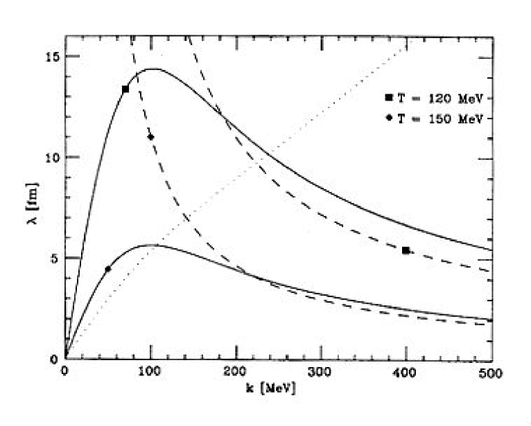
Figure 7: Absorption length as a function of pion momentum. The dashed lines describe the behavior in chiral limit, the solid lines correspond to the experimental value of $M_{\pi}$ and the dotted line gives the qualitative behavior in the $\lambda\phi^{4}$ theory.

Also the real part of the pion dispersion relation is modified on the two–loop level. To study this, one has to calculate the real part of the polarization operator (4.3) from the graph in Fig. 5 and also take into account the graph in Fig. 8 where the box stands for the vertices involving four momenta in the derivative expansion of the effective chiral lagrangian (4.18).

Figure 8: Contribution of four-derivative vertices in the pion polarization operator.

An explicit calculation along these lines has not yet been done so far. A. Schenk [88] calculated the thermal shift of ${\rm Re}\ \omega({\bf k})$ in a “mixed approach” : he used the virial expansion formula (4.37) and substituted there the forward scattering amplitude $T^{\pi\pi}(s)$ (and a similar 3 $\to$ 3 forward scattering amplitude which enters the term of the second order in pion density) as it follows from the chiral perturbation theory. Numerical plots for ${\rm Re}\ \omega({\bf k})$ at different temperatures assuming nonzero pion mass were drawn. Unfortunately, the results were presented in a way which makes an analytic analysis difficult.

In the old paper by Itoyama and Mueller [89] and in the recent [90], the same problem was studied in the linear sigma–model framework. A beautiful qualitative effect was discovered: the dispersion law of slow massless pions is modified to

$${\rm Re}\ \omega({\bf k})\ =\ c(T)|{\bf k}|,$$

$$c(T)\ =\ 1\ -\ \frac{4\pi^{2}}{45}\frac{T^{4}}{F_{\pi}^{2}M_{\sigma}^{2}}$$ (4.45)

where $M_{\sigma}$ is the mass of $\sigma$–meson which was assumed to be small compared to $2\pi F_{\pi}$. A “refraction index” appears. It is not clear for us now whether this result is reproduced also in the nonlinear sigma–model [If it is, the correction should be of order $T^{4}/F_{\pi}^{4}$ with a possible dependence on the coefficients of higher–derivative terms in (4.18)]. But I do not see a reason why it should not.

In [90] also the two–loop contribution to the residue $F_{\pi}(T)$ in (4.28) was calculated and the validity of the Gell-Mann – Oakes – Renner relation (4.15) to the order $\sim T^{4}$ was checked.

4.4 Nucleons.

Not only pions but also other hadron states change their properties when temperature is switched on. Nucleons, vector mesons etc. are not easily excited when the temperature is small, but still it makes sense to study the problem of propagation of a massive state in pion gas and find out how the presence of the thermal heat bath affects its dispersive properties. Such a study was first carried out for nucleons in [91].

We restrict ourselves with the case when the nucleon is at rest and will be interested with the temperature dependence of the pole position of the nucleon Green’s function $\Omega_{N}^{T}({\bf 0})\equiv M_{N}^{T}-i\zeta_{N}^{T}$. The real part of the pole will be called the  temperature–dependent  nucleon  mass and the imaginary part $\zeta_{N}(T)$ — the nucleon damping rate.

What we need to know is the nucleon polarization operator at finite temperature. Virial expansion in the pion density is very handy here. In the first order in density, the polarization operator is given by the graph of the same form as in Fig. 6 and, quite analogously to Eq. (4.37), we obtain

$$M_{N}^{T}-i\zeta_{N}^{T}=M_{N}^{0}+\frac{{\rm Tr}[(\gamma^{0}+1)\Sigma_{R}^{N}(M_{N}^{0},{\bf 0})]}{2}=M^{0}_{N}-\sum_{\pi^{\pm},\pi^{0}}\int\frac{d^{3}p}{(2\pi)^{3}2E}n_{B}(E)\frac{T_{\pi N}(E)}{2M_{N}^{0}},$$ (4.46)

$E=\sqrt{M_{\pi}^{2}+{\bf p}^{2}}$. $\pi N$ scattering is very well studied in experiment. We may use the available phenomenological information [95, 96] on the $\pi N$ scattering amplitude and need not come to grips with evaluating it in the chiral perturbation theory framework. The only assumption in (4.46) is that the heat bath include only pions and that their density is small enough for the virial expansion to be justified. In reality, these conditions are fulfilled up to $T\sim 130\ {\rm MeV}$. The limitations are the same as for the mesonic sector.

Consider first the damping rate. According to the optical theorem, the imaginary part of the forward scattering amplitude is related to the total cross section,

$${\rm Im}T_{\pi N}(E)\ =\ 2M_{N}^{0}\sqrt{E^{2}-M_{\pi}^{2}}\ \sigma^{\pi N}(E)$$ (4.47)

We have

$$\zeta_{N}^{T}\ =\ \frac{1}{4\pi^{2}}\int_{M_{\pi}}^{\infty}dE\ \frac{E^{2}-M_{\pi}^{2}}{e^{\beta E}-1}\left[\sigma_{\pi^{+}p}(E)+\sigma_{\pi^{0}p}(E)+\sigma_{\pi^{-}p}(E)\right]$$ (4.48)

To evaluate the integral, we insert the experimental cross section, which in the energy region of interest is dominated by the $\Delta$–resonance. In the narrow resonance limit, this gives

$$\zeta_{N}^{T}\ =\ \frac{1}{8\pi}\Gamma_{r}\sigma_{r}\frac{E_{r}^{2}-M_{\pi}^{2}}{e^{\beta E_{r}}-1}$$ (4.49)

where $\Gamma_{r}=115\ {\rm MeV}$ is the width of the resonance and $E_{r}\approx 330{\rm MeV}$ is the corresponding pion lab energy. At the peak of the resonance, the cross section saturates the unitarity limit, $\sigma_{r}^{\pi^{+}p}=8\pi/(q_{r})^{2}$, where $q_{r}$ is the c.m. momentum at resonance. Using the isospin ratios $\sigma_{r}^{\pi^{+}p}:\sigma_{r}^{\pi^{0}p}:\sigma_{r}^{\pi^{-}p}=1:\frac{2}{3}:\frac{1}{3}$, this implies $\sigma_{r}\approx 380\ {\rm mb}$. Eq. (4.49) is plotted in Fig. 9 (dashed line) together with a numerical evaluation of Eq. (4.48), based on the Karlsruhe–Helsinki data [95] (full line). Damping rapidly grows with temperature.

Figure 9: Damping rate $\gamma^{T}_{N}=2\zeta^{T}_{N}$ of nucleon collective excitations as a function of temperature. The dashed line indicates the contribution due to the $\Delta$– resonance.

It is instructive to compare this result with a situation where the physics is well understood: atoms exposed to a heat bath of photons. The virial expansion in the photon density can be carried out and a formula similar to Eq.(4.48) but involving the total cross section $\sigma_{\gamma A}$ for the collision of an atom with a photon from the heat bath can be written. This cross section grows as $\omega^{4}$ at small frequencies. As a result, the atom damping grows as $T^{7}$. This estimate is correct while the temperature is still much less than the characteristic distance between atomic levels $\sim m_{e}\alpha^{2}$. If it is not the case, excitation and ionization processes set it. In other words, when the temperature of the heat bath is high enough, the atom does not live in the ground state most of the time, but is constantly excited by thermal photons and gets eventually ionized.

Also in our case, when the temperature is high enough, the nucleon does not stay in the ground state, but is constantly converted into $\Delta$ and higher excited baryon states, absorbing and emitting pions. Our calculation of the nucleon damping makes contact with reality up to the temperatures of order $T\approx 150\ {\rm MeV}$. At this temperature, the ratio of probabilities for finding the nucleon in excited state and in the ground state, respectively, is given by $4\exp[-(M_{\Delta}-M_{N})/T]\approx 0.6$. Also, at temperatures of order $150\ {\rm MeV}$ and higher, the medium contains an increasing number of massive excitations and is not adequately represented by a dilute gas of pions.

Consider now the shift of the real part of the pole $M_{N}^{T}$ compared to its zero temperature value. We use again the virial expansion formula (4.46). The real part of the forward $\pi N$ scattering amplitude involves the Adler zero: in the chiral limit, it behaves as $\propto E^{2}$ when the energy of an ingoing pion is small. As a result, the thermal shift of the nucleon mass is proportional to $T^{4}$ at small temperatures.

Note that the term $\propto T^{2}$ is absent here in contrast to what we had for the quark condensate (4.24) and $F_{\pi}$ (4.29). It particular, early attempts [97] to use directly the Ioffe formula for the nucleon mass [98] derived from $QCD$ sum rules

$$M_{N}\ \approx\ 1.2(4\pi^{2}\Sigma)^{1/3}$$ (4.50)

and substitute there the temperature dependent condensate (4.24) are not justified. Speaking of the pion mass, its relative shift $(M_{\pi}^{T}-M_{\pi}^{0})/M_{\pi}^{0}$ is of order $T^{2}/F_{\pi}^{2}$, but, as $M_{\pi}$ is small, the absolute value of the shift is also small, and there is no shift at all in the chiral limit.

Like the damping rate, the shift of the nucleon mass can be determined from the formula (4.46) without invoking chiral theory, but using the available experimental information on the $\pi N$ forward scattering amplitude [95]. The result is shown in Fig. 10. For comparison, we also plot the chiral perturbation theory result for the temperature dependence of the pion mass (4.26).

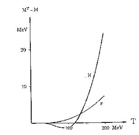
Figure 10: Shift in the effective nucleon and pion masses caused by temperature.

The main feature here is that the shift in the real part of the nucleon pole position is small compared to the shift in the imaginary part in the region of applicability of the whole approach. This finding of [91] was confirmed in recent [104].

Pion exhibits itself as a pole in the axial current correlator (4.28). Likewise, a nucleon exhibits itself as a pole in a correlator of currents with nucleon quantum numbers. If we restrict ourselves with the currents not involving derivatives of the quark fields, two choices are possible [98],

$$\eta_{1}(x)\ =\ \epsilon^{abc}\left\{\left[(u_{R}^{a})^{T}Cd_{R}^{b}\right]u_{L}^{c}\ -\ \left[(u_{L}^{a})^{T}Cd_{L}^{b}\right]u_{R}^{c}\right\},$$

$$\eta_{2}(x)\ =\ \epsilon^{abc}\left\{\left[(u_{R}^{a})^{T}Cd_{R}^{b}\right]u_{R}^{c}\ -\ \left[(u_{L}^{a})^{T}Cd_{L}^{b}\right]u_{L}^{c}\right\}$$ (4.51)

where $C$ is the charge conjugation matrix, $\gamma_{\mu}^{T}=-C\gamma_{\mu}C^{-1}$.

Figure 11: Renormalization of the nucleon residue. Dashed lines stand for pions.

Finite temperature brings about the renormalization of the residues of these currents in the nucleon states $\lambda$ by the same token as it brings about the renormalization of the residue of the axial current $F_{\pi}$. (while the current $\eta_{1}(x)$ plays a preferred role in the context of $QCD$ sum rules [98], the temperature effects on the residue of these two currents are the same). The corresponding graphs, which exactly correspond to the graphs in Fig. 4 in the pion case, are shown in Fig. 11 . Using the Goldberger–Treiman relation and the current algebra relation for the soft pion vertex $<0|\eta|\pi\pi N>$,

$$<0|\eta|N\pi^{a}\pi^{b}>\ =\ -\frac{\delta^{ab}}{4F_{\pi}^{2}}<0|\eta|N>,$$ (4.52)

and calculating the graphs in Fig. 11 in the same way as we did it earlier for pions, we arrive at the low temperature theorem [91]

$$\lambda^{T}\ =\ \lambda^{0}\left\{1\ -\ \frac{g_{A}^{2}+1}{32}\frac{T^{2}}{F_{\pi}^{2}}\ +\ \ldots\right\}$$ (4.53)

Like $F_{\pi}$, the residue drops with temperature.

One can also derive similar formulae for other hadrons. For example, $F_{K}^{T}=F_{K}(1-T^{2}/32F_{\pi}^{2}+\ldots)$, etc.

4.5 Vector mesons. Experiment.

Let us ask now whether the theoretical results presented in the two last sections can be directly confronted with experimental data in heavy ion collisions. Unfortunately, the answer is negative.

We hasten to comment that the pole positions of the collective excitations with pion and nucleon quantum numbers are quite physical quantities and can be measured in a gedanken experiment.

Suppose we study the spectrum of invariant masses of two $\gamma$ emitted from hot hadronic matter. The spectrum has a sharp peak associated with the $\pi^{0}\to 2\gamma$ decay. For free pions, the width of the peak is very small $\Gamma_{\pi}^{0}\approx 8\ eV$. But thermal pions have a finite width $\Gamma_{\pi}^{T}=2\zeta_{\pi}^{T}$ where $\zeta_{\pi}^{T}$ is the thermal average of the expression (4.3) for $\zeta_{\pi}(k)$. Also the maximum of the resonance is shifted towards larger mass values according to Eq.(4.26). Likewise, for nucleons. Proton is believed to decay eventually, and most of the decay modes (like $e^{+}\pi^{0}$) involve hadrons which are stuck within the hadronic medium and do not go out undisturbed, but there is also a mode $e^{+}\gamma$. For the argument sake, let us assume that $e^{+}$ and $\gamma$ do not interact with the heat bath, but only with detector. Measuring the distribution in invariant masses of $e^{+}\gamma$ and focusing on the “nucleon resonance”, one could, in principle, extract information on the position of the nucleon pole.

Of course, these gedanken experiments are quite unrealistic. Not even speaking of the “nucleon resonance experiment” which is a pure science fiction, also the studying of $2\gamma$ spectrum in heavy ion collisions would provide little information about pion properties in heat bath. The matter is that $\pi^{0}$ lifetime is at least six orders of magnitude larger than the lifetime of the fireball produced in the collision of heavy nuclei . Pions would decay on flight in vacuum and their mass and width would be the same as in any other experiment.

As far as experiment is concerned, the situation is much better for vector mesons, especially for $\rho$–meson. Its vacuum lifetime is pretty small, almost all $\rho$-s produced in the collision decay inside the fireball, and measuring the spectra of $e^{+}e^{-}$ or $\mu^{+}\mu^{-}$ pairs can provide an information about the properties of $\rho$ in hot hadron medium. Things are not so good with $\omega$ and $\phi$ mesons. Lifetime of hadronic fireball is estimated to be 25 fm/c or less [105]. It is of the same order as the $\omega$ lifetime and almost 2 times less than $\phi$ lifetime. A considerable fraction of $\omega$-s and most of $\phi$-s would decay outside the fireball.

Unfortunately, Life and Nature usually ingeniously resist our attempts to eliminate Trouble and put things in Order. A manifestation of this general Law in this particular case is that the problem to describe $\rho$–meson in hot matter involves much more theoretical uncertainties than in the pion or nucleon cases. The most straightforward way to study the position of $\rho$ pole is to perform virial expansion in the pion density and to write the formula like (4.37), (4.46) involving the forward $\pi\rho$ scattering amplitude $T_{\pi\rho}$. The Trouble here is that the experimental information on $T_{\pi\rho}$ is not available. We have to calculate it in some theoretical model, and that brings about uncertainties.

Something can be said, however. First of all, the amplitude of pion forward scattering on any hadron $h$ involves the Adler zero due to Goldstone nature of pion. In the chiral limit, this amplitude summed over all pion species behaves as

$$T_{\pi^{+}h}+T_{\pi^{0}h}+T_{\pi^{-}h}(E)\ \sim\ \frac{E^{2}}{\mu_{\rm hadr}^{2}}\left(A+iB\frac{|E|}{\mu_{\rm hadr}}\right)$$ (4.54)

where $\mu_{\rm hadr}$ is some characteristic hadron scale, and we assumed that the hadron $h$ has a nonzero isospin. It applies also to $\rho$. And that means that, like in the nucleon case, the real part of the $\rho$ mass shift does not have a contribution $\sim T^{2}$ in the chiral limit.

The same conclusion can be reached considering the correlators of vector and axial currents in pion heat bath. Some complication there is that the correlators themselves are shifted in the order $\sim T^{2}$, but an accurate analysis displays that this shift occurs not due to a shift of $\rho$ and $A_{1}$ poles, but due to admixture of the graph with $A_{1}$ pole in the vector correlator and the admixture of the graph with $\rho$ pole in the axial correlator [106].

However, $\rho$–meson mass is shifted in the order $\sim T^{4}$. It cannot be excluded right now that its temperature dependence is more profound than for the nucleon mass (Fig. 10 shows that the latter is almost constant in the region $T\ ^{<}_{\sim}\ 150\ MeV$ where the whole approach based on the virial expansion is justified), and it can, in principle, be essentially modified at temperatures $T^{>}_{\sim}100--150$ MeV. Whether it is modified, indeed, and, if it is, does it eventually grow with temperature [107] or decreases [108, 109] — is the question under discussion now.

Experimental data on dilepton mass spectra in heavy ion collisions [110, 111] favor more the possibility that the effective mass of $\rho$ decreases with temperature. Experimentalists observe an excess of dilepton pairs in the small invariant mass region in nucleus–nucleus collisions compared to the spectrum in proton–nucleus collisions. It seems that this excess cannot be explained in a conservative framework, with the processes of direct dilepton production in the hadronic fireball like $\pi\pi\to\rho l^{+}l^{-}$ or $\pi\rho\to\pi l^{+}l^{-}$ [112, 113]. The assumption that $M_{\rho}$ drops with temperature can explain it [109, 113].

5 Chiral symmetry restoration.

5.1 General considerations. Order of phase transition and critical behavior.

In $QCD$ with 2,3, and possibly 4 massless quark flavors (see the discussion in Sect. 4.1), chiral symmetry is spontaneously broken at zero temperature. In the preceding chapter, we studied the dynamics of the system at comparatively low temperatures when chiral symmetry is still broken, and the spectrum of the system involves massless Goldstone states. But a spontaneously broken symmetry is usually restored under sufficient heating, like a spontaneously broken rotational symmetry in ferromagnet is restored above the Curie point.

There are few exceptions of this general rule. First of all, it does not apply to supersymmetry. Supersymmetry is always broken spontaneously at nonzero temperature irrespectively of whether it is broken or not at $T=0$. The most immediate way to see it is to notice that different boundary conditions in Euclidean time in the Matsubara formalism, periodic for bosons and antiperiodic for fermions, are not invariant under supersymmetry transformations which mix bosonic and fermionic fields. This is also seen in the real time hamiltonian formalism. The standard density matrix $\exp\{-\beta H\}$ is transformed under supersymmetry transformation into $\exp\{-\beta(H-Q\bar{\epsilon}-\epsilon\bar{Q})\}$ where the parameters of SUSY transformation $\bar{\epsilon}$, $\epsilon$ have the meaning of chemical potentials corresponding to conserved supercharges $Q$, $\bar{Q}$ [114]. Supersymmetry is spontaneously broken by the same reason why the Lorentz symmetry is spontaneously broken at finite $T$. In the latter case, the density matrix is non-trivially transformed under the Lorentz boost and acquires the form $\exp\{-\beta(H-{\bf v}{\bf P})/\sqrt{1-{\bf v}^{2}}\}$ where ${\bf P}$ are conserved momenta and the velocity ${\bf v}$ plays the role of corresponding chemical potentials.

Supersymmetry is a special case, but there are also some systems where spontaneous breaking of a usual (bosonic) global symmetry persists until arbitrary high temperatures. Moreover, heating the system can even induce the spontaneous breaking which was absent at zero temperature [34]. Such systems are, however, rather exotic, and there are some special dynamic reasons for this peculiar phenomenon. There are no such reasons in $QCD$, it behaves as most of the physical systems do, and that means that a critical temperature $T_{c}$ exists above which the chiral symmetry is restored and the fermion condensate $<\bar{q}q>_{T}$ is zero. This is the temperature of phase transition and $<\bar{q}q>_{T}$ is the order parameter associated with the transition.

Note that the statement of the existence of the phase transition point does not apply to the theory with only one massless flavor. As was already noted in Sect. 4.1, quark condensate does not signal there a spontaneous symmetry breaking [$U_{A}(1)$ symmetry is anyway broken explicitly by anomaly], is not an order parameter, and need not vanish at high temperature. So, it does not. At high temperatures when the effective coupling is small, it can be evaluated semi-classically in the instanton approach [5, 115], and one can show that it falls down as a power of temperature and never reaches zero.

Let us return to the case of several massless flavors when spontaneously broken chiral symmetry is restored at some temperature. The first question to be asked is what is the order of this phase transition, i.e. whether the order parameter $<\bar{q}q>_{T}$ itself, or only its derivative $\partial<\bar{q}q>_{T}/\partial T$ are discontinuous at the phase transition point.

This question can be studied theoretically. There are rather suggestive arguments which indicate that the phase transition is of the second order for 2 massless flavors. When $N_{f}\geq 3$, the phase transition is probably of the first order. (If it is there, of course. We mentioned earlier that, for $N_{f}\geq 4,5$, chiral symmetry is probably not broken at all, and there is nothing to be restored.) The arguments are the following [116]:

The starting point is the observation that, in theories involving scalar fields, phase transition of the first order often occurs when the potential involves a cubic in fields term. One can recall in the first place a cubic Van-der- Vaals curve $P(\rho,T)$ which describe the first order water $\leftrightarrow$ vapor phase transition. The simplest field theory example is the theory of real scalar field with the potential

$$V(\phi)=\lambda(\phi^{2}-v^{2})^{2}-\mu\phi^{3}$$ (5.1)

Assume for simplicity $\mu\ll\lambda v$. At $T=0$, the potential has one global minimum at $\phi\approx v+3\mu/8\lambda$ and a local minimum at $\phi\approx-v+3\mu/8\lambda$. At nonzero temperature, the term $\sim\lambda T^{2}\phi^{2}$ is added to the effective potential. At high temperature $T\gg v$, the only minimum occurs at $\phi=0$. One can be easily convinced that, as the temperature increases, the left local minimum moves on the right and reaches the point $\phi=0$ (after which it does not move anymore) at some temperature $T^{*}$ when the global minimum at positive $\phi$ still exists. When the temperature is further increased, the right minimum moves up and becomes degenerate with the minimum at $\phi=0$ at some temperature $T_{c}$. The former disappears altogether at a still larger larger temperature $T^{**}$. In a certain temperature range, two minima of the potential coexist, one being a metastable state with respect to the other. This is exactly the physical situation of the first order phase transition.

Let us go back to $QCD$. A direct application of this reasoning is not possible because the $QCD$ lagrangian does not involve scalar fields. The effective chiral lagrangian (4.18) is also of no immediate use because higher-derivative terms which stand for dots cannot be neglected in the region close to critical temperature. Suppose, however, that in the region $T\sim T_{c}$ some other effective lagrangian in Ginzburg-Landau spirit can be written which depends on the composite colorless fields

$$\Phi_{ff^{\prime}}=\bar{q}_{Rf}q_{Lf^{\prime}}$$ (5.2)

A general form of the effective potential which is invariant under $SU_{L}(N_{f})\otimes SU_{R}(N_{f})$ is

$$V[\Phi]\sim g_{1}{\rm Tr}\{\Phi\Phi^{\dagger}\}+g_{2}({\rm Tr}\{\Phi\Phi^{\dagger}\})^{2}$$

$$+g_{3}{\rm Tr}\{\Phi\Phi^{\dagger}\Phi\Phi^{\dagger}\}+g_{4}(\det\Phi+\det\Phi^{\dagger})+\ldots$$ (5.3)

(the coefficients may be smooth functions of $T$). Now look at the determinant term. For $N_{f}=2$, it is quadratic in fields while, for $N_{f}=3$, it is cubic in fields and the effective potential acquires the structure similar to Eq.(5.1) which is characteristic for the systems with first order phase transition. A more refined analysis [116] shows that the first order phase transition is allowed also for $N_{f}\geq 4$, but not for $N_{f}=2$ where the phase transition is of the second order.

Most of the existing lattice data [117, 118, 119] indicate that, at $N_{f}=3$, the phase transition is of the first order, indeed, while, at $N_{f}=2$, it is of the second order. The latter is not, however, a generally accepted statement yet, and the discussion on this issue is still alive (we will discuss lattice data in some more details a bit later).

Critical behavior

A second order phase transition is characterized by critical behavior, i. e. a power–like scaling behavior of the specific heat, the expectation value of the order parameter, and the correlators. Different critical exponents can be defined.

Let us list them briefly here (for more details, see e.g. Chapter XXIV in [120]). Suppose we have a system with an order parameter $<\phi>$ which turns to zero at the second order phase transition point. Introduce also a weak external field $h$ which is canonically conjugate to $\phi$. For standard ferromagnet, $<\phi>$ is magnetization and $h$ is the magnetic field. For $QCD$, $<\phi>$ is the quark condensate and $h$ is the small common quark mass.

The exponent $\alpha$ is related to the scaling behavior of the specific heat $c_{P}(T)$ slightly above or slightly below a critical temperature:

$$c_{P}(T)\ =\ A_{\alpha}^{\pm}|T-T_{c}|^{-\alpha}$$ (5.4)

The coefficients $A_{\alpha}^{\pm}$ are called critical amplitudes and the index + or - refers to whether we are dealing with the system in the disordered phase $T>T_{c}$ or in the ordered phase $T<T_{c}$.

The scaling behavior of $c_{P}$ at $T=T_{c}$ but at nonzero external field $h$ is determined by the critical exponent $\epsilon$:

$$c_{P}(h)\ =\ A_{\epsilon}h^{-\epsilon}$$ (5.5)

When we approach $T_{c}$ from below, the order parameter tends to zero as a power

$$<\phi>_{T}\ =\ A_{\beta}(T_{c}-T)^{\beta}$$ (5.6)

At $T=T_{c}$ and $h\neq 0$, the order parameter also exhibits a power–like behavior

$$<\phi>_{h}\ =\ A_{\delta}h^{1/\delta}$$ (5.7)

When $T\neq T_{c}$, the shift in $<\phi>$ provided by the external field $h$ is proportional to $h$. The proportionality coefficient is called the generalized susceptibility $\chi$ which scales as

$$\chi\ =\ A_{\gamma}^{\pm}|T-T_{c}|^{-\gamma}$$ (5.8)

At $T=T_{c}$ and $h=0$, the mass gap in the physical spectrum is absent and the correlation length is infinite. The correlator of the order parameters falls down at large distances as a power

$$<\phi({\bf x})\phi(0)>_{T=T_{c},h=0}\ =\ A_{\zeta}|{\bf x}|^{-(d-2+\zeta)}$$ (5.9)

where $d$ is the spatial dimension. At $T\neq T_{c}$ and/or $h\neq 0$, the mass gap appears. It scales as

$$M_{\rm gap}\ =\ A_{\mu}h^{\mu},\ \ \ \ \ \ \ \ \ \ \ T=T_{c},\ h\neq 0$$ (5.10)

and

$$M_{\rm gap}\ =\ A_{\nu}^{\pm}|T-T_{c}|^{\nu},\ \ \ \ \ \ \ \ \ \ \ T\neq T_{c},\ h=0$$ (5.11)

Eight critical exponents $\alpha,\beta,\gamma,\delta,\epsilon,\zeta,\mu,\nu,$ are related by six scaling relations (so that only two of them are independent parameters):

$$\alpha+2\beta+\gamma\ =\ 2,\ \ \ \ \ \ \ \ \beta\delta\ =\ \beta+\gamma,$$

$$\epsilon(\beta+\gamma)\ =\ \alpha,\ \ \ \ \ \ \ \ \ \ \mu(\beta+\gamma)\ =\ \nu,$$

$$\nu(2-\zeta)\ =\ \gamma,\ \ \ \ \ \ \ \ \ \ \nu d\ =\ 2-\alpha$$ (5.12)

A very important property of the critical exponents is their universality. That means that the values of $\alpha,\beta$ etc. do not depend on the details of microscopic hamiltonian, but only on gross symmetry features of the theory. It follows basically from the fact that critical behavior is determined by the dynamics of the theory at distances which are much larger than the microscopic scale (much larger than $1/\mu_{\rm hadr}$ in our case). At the critical point, the effective theory describing large–distance dynamics is a conformal theory not involving any dimensional parameter. At the vicinity of critical point, it is a perturbed conformal theory corresponding to adding to the effective lagrangian an energy operator or an order parameter operator with small coefficients. The effective theory thus obtained involves now a mass scale , but as long as it is small compared to a characteristic energy scale in the microscopic hamiltonian ($\mu_{\rm hadr}$), this effective theory is still universal.

And that means that, in order to determine the critical exponents in $QCD$ with 2 light quarks at the vicinity of the second order phase transition point, we need not to deal explicitly with $QCD$ which is a complicated theory, but are allowed to consider some other theory belonging to the same universality class, i.e. with the same symmetry breaking pattern. The exponents will be same. The universality class of $QCD$ with $N_{f}=2$ corresponds to the symmetry breaking pattern $SU_{L}(2)\otimes SU_{R}(2)\to SU(2)$ which is the same as $O(4)\to O(3)$. A rather simple example of the theory in this universality class is the so called Heisenberg $O(4)$ magnet (Imagine a 3–dimensional cubic lattice involving 4–dimensional spin variable $S_{\mu}$ at each node. The hamiltonian is the interaction $S_{\mu}S^{\prime}_{\mu}$ for all nearest neighbors). At low temperatures, spins are ordered $<S_{\mu}>_{T=0}\neq 0$. When temperature is increased, the system undergoes a second order phase transition and goes over into the disordered phase. The values of critical exponents in this model are known [121] (they were obtained in $\epsilon$ expansion technique). The universality argument tells us that their values in $QCD$ are exactly the same [122, 123]. Specifically,

$$\alpha\ =\ -.19\pm.06,\ \ \beta\ =\ .38\pm.01,\ \ \gamma\ =\ 1.44\pm.04,\ \ \delta\ =\ 4.82\pm.05,$$

$$\epsilon\ =\ -.10\pm.03,\ \ \zeta\ =\ .03\pm.01,\ \ \mu\ =\ .40\pm.02,\ \ \nu\ =\ .73\pm.02$$ (5.13)

A distinct feature of the model is the negative value of $\alpha$ so that the specific heat does not diverge at the critical temperature, but rather goes to zero with a cusp.

The predictions (5.1) can be confronted with experimental lattice data. At the moment, an experimental situation is uncertain. The values of the exponents determined in [124] agree with the theory rather well. In particular, their result $\delta^{-1}=.24\pm.03$ coincides with the theoretical prediction within the error bars. This finding was confirmed in recent [125] by another group. However, a preferred value for $\delta^{-1}$ given in a later work of the Bielefeld group done on larger lattices [126] is close to zero which actually indicates that the phase transition observed is of the first order and which sharply contradicts theoretical expectations. Also nobody has seen the predicted cuspy zero for the specific heat so far. One has to mention also the recent work [127] where critical exponents were measured in 2+1 – dimensional Gross–Neveu model. (Like $QCD$, it involves light fermions and enjoys a chiral symmetry. Like in $QCD$, chiral symmetry is broken spontaneously at zero temperature and is restored at high temperature) The values of the exponents measured in [127] do not conform with the predictions based on universality and the $\epsilon$–expansion (which is rather surprising as these predictions work remarkably well in the condensed matter systems where laboratory experimental information is in abundance), but are instead rather close to the values predicted in the Landau mean field model.

Being not a lattice expert, I cannot judge, of course, who is right and who is wrong. Four–dimensional calculations are complicated. The most modern, specially dedicated for this purpose computers should work for hundreds of hours to produce statistically reliable results.

However, there are also systematic errors in any experiment. Taking them under control depends on the skill of an experimentalist, and a layman has no say in that. The situation is much better when the experiment can be gauged, i.e. performed in the region where some solid theoretical results exist. If something known is reproduced in experiment with good accuracy, one can trust the experiment also when Unknown is measured. Fortunately, such a possibility (which has not been yet fully exploited) does exist for lattice numerical calculations. I mean here certain 2–dimensional models involving fermions where exact theoretical predictions can be made and where, on the other hand, lattice calculations are much more easy and require much less computer time.

That refers in particular to Schwinger model (i.e. 2–dimensional $QED$) with several ( $N_{f}>1$) light fermion flavors. Much like as $QCD$, this model enjoys the chiral symmetry $SU_{L}(N_{f})\otimes SU_{R}(N_{f})$. In two dimensions, a continuous symmetry cannot be broken spontaneously due to the Mermin – Wagner – Coleman theorem [128]. So it does not and the quark condensate is zero in the massless theory. It can be shown, however, that at small temperatures and small fermion masses, the system displays a critical behavior like a system with second order phase transition at temperatures slightly above critical. One can say that the second order phase transition occurs at zero temperature (so that there is no ordered phase, indeed) [129]. The exact values of critical exponents can be determined. They are [130]

$$\alpha=-1,\ \ \gamma=\frac{2}{N_{f}},\ \ \delta=\frac{N_{f}+1}{N_{f}-1},\ \ \mu=\frac{N_{f}}{N_{f}+1},\ \ \nu=1,\ \ \zeta=2-\frac{2}{N_{f}}$$ (5.14)

When $N_{f}=2$, also, critical amplitudes entering (5.4) - (5.9) can be exactly calculated [131]. In particular,

$$<\bar{\psi}_{1}\psi_{1}>_{T=0}\ =\ <\bar{\psi}_{2}\psi_{2}>_{T=0}\ =\ -.388\ldots m^{1/3}g^{2/3},$$

$$M_{\rm gap}\ =\ 2.008\ldots m^{2/3}g^{1/3}$$ (5.15)

There is only one comparatively old lattice paper where Schwinger model with 2 flavors was studied [132]. The measured values of the critical exponents agree well with theoretical predictions. However, the experimental values of the critical amplitudes exceed their theoretical values by 35% for the condensate and by 25% for the mass gap. It would be very interesting, indeed, to repeat this calculation on modern computers and with different modern lattice algorithms (Wilson vs. Kogut–Susskind fermions, perfect vs. improved vs. simple–minded actions etc.). Confirmation of the theoretical predictions (5.14, 5.1) with good accuracy would provide an efficient test of lattice methods.

5.2 Insights from soft pion physics. Large $N_{c}$.

We have already seen an indication for the chiral symmetry restoration in the previous chapter: according to Eq.(4.24), the order parameter $\Sigma(T)=-<\bar{q}q>_{T}$ decreases as the temperature is increased. That was a one–loop calculation which had only a limited range of validity $T<\ 80-100\ MeV$ where the temperature correction is still small. One can, however, improve the accuracy and find out the temperature dependence of the condensate on the 2–loop and 3–loop level in chiral perturbation theory. This calculation done in [83, 84] allows one to monitor melting down of the quark condensate at larger temperatures and make a reasonable estimate for the temperature of phase transition where the condensate disappears.

Figure 12: Two loop contribution in the pion free energy.

Figure 13: Some graphs contributing in the free energy on the three–loop level.

Let us describe the results of [84] where the temperature dependence of $<\bar{q}q>_{T}$ has been determined on the 3-loop level. To this end, one has to calculate the free energy density on the three loop level at small nonzero quark masses and differentiate the result over the quark mass. There is only one relevant two–loop graph depicted in Fig. 12. By a simple power counting [We have $T^{2}M_{\pi}^{2}\sim\Sigma m(T^{2}/F_{\pi}^{2})$ from the pion mass dependent term in the free energy and an additional factor $\sim T^{2}/F_{\pi}^{2}$ from the vertex (4.1) involving two derivatives, i.e. the square of a characteristic momentum $p_{\rm char}\sim T$ of pions in the thermal loop ], it gives the correction $\sim T^{4}/F_{\pi}^{4}$ in the condensate. There are many 3–loop graphs. We will depict two of them. The graph in Fig. 13a involves only the standard 4–pion vertex (4.1) and depends only on $F_{\pi}$ (it depends also on the ultraviolet cutoff, but disregard it for a moment). The graph in Fig. 13b contains something new. It looks as a two–loop graph, but contributes actually in the order $\sim T^{6}$ because the square vertex in this graph stands for the terms in the effective lagrangian (4.18) involving four derivatives. There are several chiral invariant structures of this kind. One of them has the form

$${\cal L}^{(4)}\ =\ \alpha\left({\rm Tr}\left\{\partial_{\mu}U^{\dagger}\partial_{\mu}U\right\}\right)^{2}$$ (5.16)

The dimensionless coefficient $\alpha$ (another name for it is $L_{1}$ [80]) is a new independent parameter of the lagrangian. In this order, there are 4 more such new dimensionless coefficients $L_{2,3,4,5}$ which are relevant to our problem. All of them affect the temperature renormalization of the condensate in the order $\sim T^{6}$. These new parameters are largely fixed, however, from experimental data on pion (and also $K$, $\eta$ ) interactions at intermediate range of energies which are also affected by $L_{i}$ [81]. The final result for the condensate in massless theory in soft pion approximation (i.e. when the effects due to $K$ and $\eta$ are disregarded together with effects coming from other resonances) has a rather simple form

$$<\bar{q}q>_{T}=<\bar{q}q>_{0}\left[1-\frac{T^{2}}{8F_{\pi}^{2}}-\frac{T^{4}}{384F_{\pi}^{4}}-\frac{T^{6}}{288F_{\pi}^{6}}\ln\frac{\Lambda}{T}+\ldots\right]$$ (5.17)

Here all effects from the higher-derivative term are described by the constant $\Lambda$. Experimental data on pseudogoldstone interactions give the value $\Lambda\sim 500\pm 100$ Mev. The dependence (5.17) together with the curves where only the 1-loop correction $\propto T^{2}$ or also the 2-loop correction $\propto T^{4}$ are taken into account (please, do not put attention to the “technical” curve marked $a^{0}_{2}=0$) is drawn in Fig. 14 taken from Ref. [84].

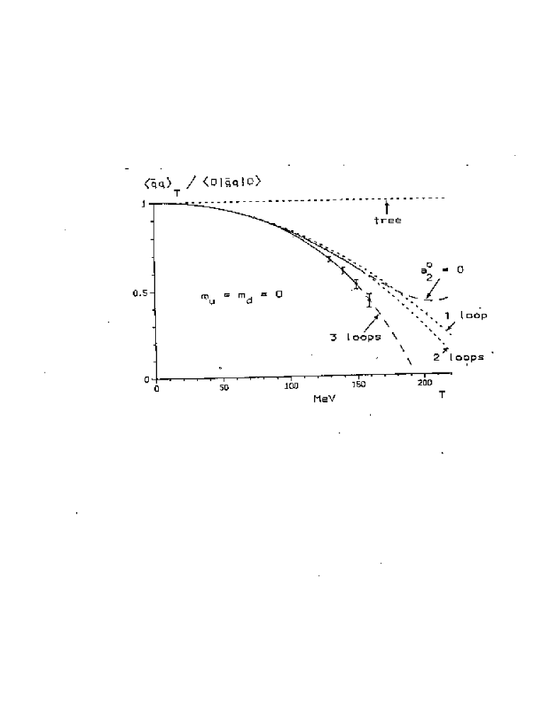
Figure 14: Temperature dependence of the condensate in three loops.

The expansion in the parameter $\sim T^{2}/8F_{\pi}^{2}$ makes sense when this parameter is small, i.e. when $T\ ^{<}_{\sim}\ 100-150$ Mev. Strictly speaking, one cannot extrapolate the dependence (5.17) for larger temperatures, especially having in mind that, at $T>150$ Mev, the heat bath includes a considerable fraction of other than pion hadron states. But as we know anyhow that the phase transition with restoration of chiral symmetry should occur, the estimate of the phase transition temperature (i.e. the temperature when $<\bar{q}q>_{T}$ hits zero, and we assume here that $N_{f}=2$ so that the transition is of the second order) based on such an extrapolation is not altogether stupid. This estimate is

$$T_{c}\approx 190\ {\rm Mev}$$ (5.18)

or, roughly, one inverse fermi. A more accurate treatment which takes into account nonzero $m_{u,d}$ and also the presence of other mesons in the heat bath gives practically the same estimate for the phase transition temperature (assuming, of course, that the phase transition is there which, as we will see in the next section, is probably not the case): nonzero quark masses smoothen the temperature dependence of the condensate and push $T_{c}$ up while excitation of other degrees of freedom sharpen the temperature dependence and pulls it down. These two effects practically cancel each other.

Large $N_{c}$.

It is interesting to discuss what happens in the large $N_{c}$ limit [46]. As usual, we assume $N_{c}\to\infty,\ \ g^{2}\to 0$ such that the product $g^{2}N_{c}$ stays constant. For simplicity, we also assume zero quark masses.

In this limit, the spectrum of $QCD$ presents a set of infinitely narrow meson resonances. In the first place, we have $N_{f}^{2}$ massless Goldstone states. An additional Goldstone particle is $\eta^{\prime}$. When $N_{c}$ is finite, $\eta^{\prime}$ is massive because $U_{A}(1)$ axial symmetry of the $QCD$ lagrangian is broken explicitly by anomaly. However, in the limit $N_{c}\to\infty$, the effects due to anomaly are suppressed, $U_{A}(1)$ becomes a good symmetry of the full quantum theory, and its spontaneous breaking by quark condensate brings about a new massless Goldstone state [133]. When $N_{c}$ is large but not infinite, the mass of $\eta^{\prime}$–meson has the order $M_{\eta^{\prime}}\propto 1/\sqrt{N_{c}}$ [134]. Besides that, there are also massive meson excitations. The mass of the first such excitation $\equiv\mu_{\rm hadr}$ does not depend on $N_{c}$. The density of higher excited states grows exponentially with mass.

Low energy properties of $N_{f}^{2}$ Goldstone states are described by a modified chiral lagrangian which has exactly the same form as (4.18), only $U$ is now a full $U(N_{f})$ rather than $SU(N_{f})$ matrix (there is also a determinant term [134], but it is suppressed in the large $N_{c}$ limit). The temperature corrections to the quark condensate can be calculated by the same token as earlier, only the coefficients are modified a little bit. In particular, the first temperature correction to the condensate (4.24) involves now the factor $N_{f}^{2}$ rather than $N_{f}^{2}-1$. A glance on the large $N_{c}$ analog of the expression (5.17) displays an apparent paradox. Indeed, $F_{\pi}$ scales as $\sqrt{N_{c}}$ in the large $N_{c}$ limit. And that seems to mean that the temperature corrections to the condensate become essential at $T\propto\sqrt{N_{c}}\mu_{\rm hadr}$. Thereby, the condensate should turn to zero and chiral symmetry be restored at $T_{c}\sim\sqrt{N_{c}}\mu_{\rm hadr}$.

This estimate for the phase transition temperature contradicts, however, physical intuition. The relevant physical scale in large $N_{c}$ theory is not $\sqrt{N_{c}}\mu_{\rm hadr}$, but just $\mu_{\rm hadr}$. In particular, in the infinite $N_{c}$ limit, the temperature $T_{c}\sim\sqrt{N_{c}}\mu_{\rm hadr}$ is much larger than the Hagedorn maximal temperature $T_{H}\sim\mu_{\rm hadr}$ and just cannot be reached (see the discussion in the beginning of Sect. 3.3).

If $N_{f}\geq 3$ (when the phase transition is of the first order), there is a way out. We may suppose that the condensate stays practically unchanged until $T_{c}$ and then abruptly jumps to zero. But in the theory with $N_{f}=2$, the phase transition is of the second order, the condensate should approach zero when we approach $T_{c}$ from below, and we do not see yet how is it possible in the soft pion framework.

The resolution of this paradox will be given in a moment, but first note that, after all, the fact that at, say, $T=T_{c}/2$ the condensate is practically not changed in the large $N_{c}$ limit compared to its zero temperature value is quite natural and reasonable. Eventually, the condensate melts down due to nonlinear pion interactions. The latter can be estimated as being due to a resonance exchange, say, $\pi\pi\to\rho\to\pi\pi$. Three–meson vertices scale as $1/\sqrt{N_{c}}$ in the large $N_{c}$ limit (this suppression brings about the suppression $\propto 1/N_{c}$ for resonance widths). Thus four–pion vertex scales as $1/N_{c}$ and, indeed, it is seen also from Eq.(4.1). On the other hand, when the temperature is increased up to $\sim\mu_{\rm hadr}$, the density of thermal pions $n\sim T^{3}$ becomes so large that the characteristic distance between pions is of the same order as their size (the latter has the order $\sim\mu_{\rm hadr}^{-1}$ and does not scale with $N_{c}$). Pions overlap, and something is bound to happen at this point.

And it does. We have seen that the correction $\propto T^{6}$ in (5.17) involves, besides $F_{\pi}$, also a new constant $\Lambda$ which describes the contribution of the graphs of the kind drawn in Fig. 13b involving higher–derivative terms in the chiral lagrangian. The corresponding dimensionless constants $L_{i}$, i = 1,…, 5 scale as $N_{c}$ [80]. (Indeed, at $p_{\rm char}\sim\mu_{\rm hadr}$, all terms in the pion lagrangian should be of the same order, and hence all coefficients in ${\cal L}^{(4)}$, ${\cal L}^{(6)}$, etc. scale in the same way as $F_{\pi}\propto N_{c}$. ). The contribution in $\Sigma(T)/\Sigma(0)$ due to the graph in Fig. 13b is estimated to be $\sim N_{c}T^{6}/F_{\pi}^{6}$, i.e., for large $N_{c}$, it dominates over the contribution coming from the graph in Fig. 13a depending only on $F_{\pi}$. Staying on the 3–loop level, we would conclude that the correction is of order 1 when $T\sim N_{c}^{1/3}\mu_{\rm hadr}$ which is better than $T\sim N_{c}^{1/2}\mu_{\rm hadr}$, but is not satisfactory yet.

However, one should, of course, include in the estimate also the contributions due to still higher order terms ${\cal L}^{(6)}$, ${\cal L}^{(8)}$, etc. Drawing the same graph as in Fig. 13, but with a 4–pion vertex coming from ${\cal L}^{(6)}$ (the corresponding coefficients scale as $N_{c}/\mu_{\rm hadr}^{2}$), we arrive at the estimate

$$\frac{\Sigma(0)-\Sigma^{\rm 4-loop}(T)}{\Sigma(0)}\ \sim\ \frac{1}{N_{c}\mu_{\rm hadr}^{3}}\ (\mu_{\rm hadr}T^{2})\ \frac{1}{F_{\pi}^{4}}\ \frac{N_{c}}{\mu_{\rm hadr}^{2}}\ T^{6}\ \sim\ \frac{T^{8}}{N_{c}^{2}\mu_{\rm hadr}^{8}}$$ (5.19)

Here the first factor is $[\Sigma(0)]^{-1}$, $\mu_{\rm hadr}T^{2}$ comes from the expansion of the free energy in pion mass $F_{M}\propto M_{\pi}^{2}T^{2}$ and its subsequent differentiation over quark mass m, $1/F_{\pi}^{4}$ comes from the expansion of $U$ up to the fourth order in $\phi^{a}$, $N_{c}/\mu_{\rm hadr}^{2}$ is the estimate of a coefficient of six–derivative term, and $T^{6}$ is the sixth power of a characteristic momentum.

Summing up the leading in $N_{c}$ terms, we obtain

$$\Sigma(T)\ \sim\ \Sigma(0)\left[1-\frac{x^{2}}{N_{c}^{2}}F(x)\right]$$ (5.20)

where $F(x)$ is some function of a dimensionless parameter $x=T^{2}/\mu_{\rm hadr}^{2}$. We do not now how the function $F(x)$ behaves at $x\ ^{>}_{\sim}\ 1$, but a quite natural assumption is that the Taylor series for this function has a finite radius of convergence so that $F(x)$ becomes infinite at some $x_{0}$. After all, the condensate is the derivative of free energy density over quark mass, and free energy definitely becomes infinite at Hagedorn temperature [see Eq.(3.18)]. Let us assume further that $F(x)$ has the simple pole at $x=x_{0}$. Now if we keep temperature fixed and send $N_{c}$ to infinity, the correction to the condensate vanishes. If, on the other hand, we keep $N_{c}$ fixed, the quark condensate (5.20) would vanish and the phase transition would occur at some point $x_{\rm crit}$ somewhat below $x_{0}$, $x_{0}-x_{\rm crit}\sim 1/N_{c}^{2}$. The characteristic width of the region where $\Sigma(T)$ is essentially changed is also estimated then as

$$\frac{\Delta T}{T_{c}}\ \sim\ \frac{1}{N_{c}^{2}}$$ (5.21)

If one assumes that $F(x\sim x_{0})\ \sim\ 1/(x-x_{0})^{2}$, the width of the transition region would be somewhat larger $\propto 1/N_{c}$. If the singularity is weaker than $1/(x-x_{0})$, the width of the transition region would be smaller (but is always suppressed at large $N_{c}$).

Thus the paradox is resolved. We see that, at $N_{f}=2$ and large $N_{c}$, the condensate is practically not changed, indeed, up to very vicinity of the phase transition point where it drops sharply and eventually hits zero. At $N_{f}\geq 3$, there is no “need” for the condensate to approach zero smoothly when the temperature approaches $T_{c}$. It can still be essentially changed in the transition region below $T_{c}$, approach some half–way value of order $\Sigma(0)/2$ and then abruptly jump to zero at the phase transition point. On the other hand, it can remain constant until the very phase transition point and then jump to zero “the whole way”. Finally, it can also approach zero when $T\to T_{c}$ and the phase transition can still be the second order. (Ginzburg–Landau arguments presented above allow the first order phase transition at $N_{f}\geq 3$ but do not dictate it to be the case.) Currently, no further conclusions on this point can be drawn.

5.3 The real world.

Up to now, we discussed only $QCD$ with massless quarks. But the quarks have nonzero masses: $m_{u}\approx$ 4 Mev, $m_{d}\approx$ 7 Mev, and $m_{s}\approx$ 150 Mev [78]. The question arises whether the nonzero masses affect the conclusion on the existence or non-existence and the properties of the phase transition.

Two different experimental (i.e. lattice) works where this question was studied are available now, and the results of these two studies drastically disagree with each other. The results of Columbia collaboration [117] display high sensitivity of the phase transition dynamics to the values of light quark masses. In Fig. 15, a phase diagram of $QCD$ with different values of quark masses $m_{s}$ and $m_{u}=m_{d}$ as drawn in Ref.[117] is plotted.

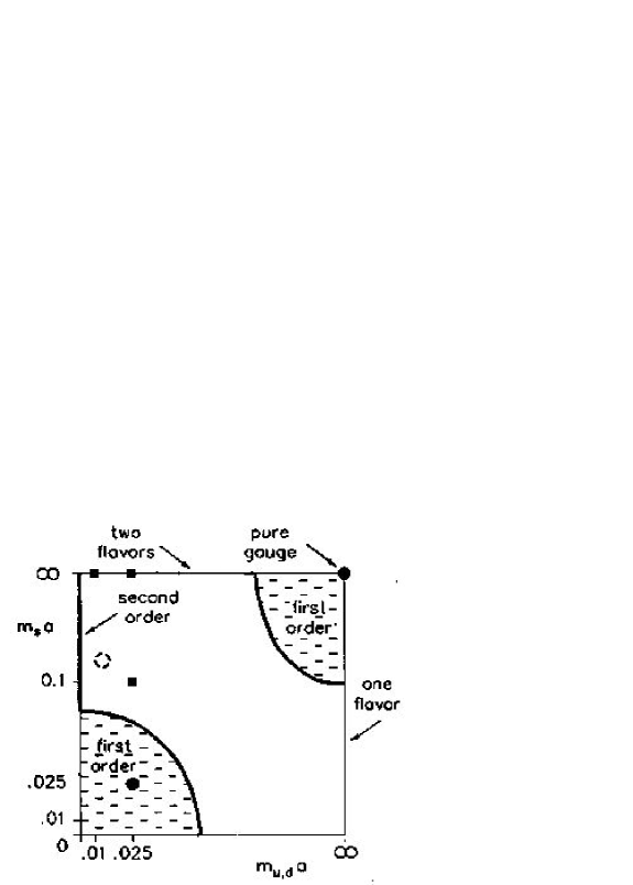
Figure 15: Phase diagram of $QCD$ according to Ref.[117]. Mass values (measured in the units of the inverse lattice spacing $a^{-1}$ for which the transition is and is not seen are denoted respectively by solid circles and squares. Dashed circle corresponds to the physical values of masses.

Let us discuss different regions on this plot. When the quark masses are large, quarks effectively decouple and we have pure YM theory with $SU(3)$ gauge group where the phase transition is of the first order. When all the quark masses are zero, the phase transition is also of the first order. When masses are shifted from zero a little bit, we still have a first order phase transition because a finite discontinuity in energy and other thermodynamic quantities cannot disappear at once when external parameters (the quark masses) are smoothly changed.

But when all the masses are nonzero and neither are too small nor too large, phase transition is absent. Notice the bold vertical line on the left. When $m_{u}=m_{d}=0$ and $m_{s}$ is not too small, we have effectively the theory with two massless quarks and the phase transition is of the second order. The experimental values of quark masses (the dashed circle in Fig.15) lie close to this line of second order phase transitions but in the region where no phase transition occurs. It is the experimental fact as measured in Ref. [117].

This statement conforms nicely with a semi-phenomenological theoretical argument of Ref. [135] which displays that even if the first order phase transition occurs in QCD, it is rather weak. The argument is based on a generalized Clausius-Clapeyron relation. In college physics, it is the relation connecting the discontinuity in free energy at the first-order phase transition point with the sensitivity of the critical temperature to pressure. The Clausius-Clapeyron relation in $QCD$ reads

$${\rm disc}<\bar{q}q>_{T_{c}}\ =\ \frac{1}{T_{c}}\ \frac{\partial T_{c}}{\partial m_{q}}{\rm disc}\ \epsilon$$ (5.22)

where ${\rm disc}\ \epsilon$ is the latent heat. The derivative $\frac{\partial T_{c}}{\partial m_{q}}$ can the estimated from theoretical and experimental information of how other essential properties of $QCD$ depend on $m_{q}$ and from the calculation of $T$ - dependence of condensate at low temperature in the framework of chiral perturbation theory (see Fig.14 and the discussion thereof). The dependence on quark masses is not too weak: $\partial T_{c}/\partial m_{q}\approx 0.9-1.0$. From that, assuming that the discontinuity in quark condensate is as large as $<\bar{q}q>_{0}$, we arrive at an estimate

$${\rm disc}\ \epsilon\ <0.4\ {\rm GeV/fm}^{3}$$ (5.23)

This upper limit for ${\rm disc}\ \epsilon$ should be compared with the characteristic energy density of the hadron medium at $T\sim T_{c}\sim 190$ MeV. The latter cannot be calculated analytically and we have to rely on numerical estimates. The lattice study in [136] (for the theory with 2 massless flavors) gives a rather large value $\epsilon(T\sim 200\ {\rm MeV})\ \approx\ 3\ {\rm GeV}/{\rm fm}^{3}$. May be, this value is even too large, it is of the same order as the Stefan–Boltzmann energy (6.1, 6.3, 6.5) of free quarks and gluons in $QGP$ phase. This is surprising as, at such low temperatures, quarks and gluons are certainly not free and the interaction effects are important — see a detailed discussion in the next chapter. Anyway, one can safely conclude that the limit (5.23) for the latent heat is several times smaller than $\epsilon(T_{c})$. In reality, the discontinuity in $<\bar{q}q>$ at the phase transition point (if it is there) is, of course, much smaller than the value of the condensate at zero temperature. It is seen from the graph in Fig.14. The condensate drops significantly still in the region where $K$ and $\eta$ degrees of freedom are not yet effectively excited. These degrees of freedom (and also $\rho$ and $\omega$ degrees of freedom) become relevant only at $T\ ^{>}_{\sim}\ 150$ MeV when the tendency of the condensate to drop down is already well established. Moreover, as was mentioned earlier in the paragraph after Eq.(5.18), taking into account these degrees of freedom sharpens the condensate dependence rather than smoothens it. This is also seen from Eq.(4.24): The more is the number of massless quark flavors $N_{f}$, the sharper is the temperature dependence of the condensate.

Thus latent heat of the first order phase transition in the theory with 3 massless quarks must be rather small [significantly smaller than the estimate (5.23)] which means that the phase transition is likely to disappear under a relatively small perturbation due to nonzero $m_{s}$. The numerical findings of Ref.[117] are thereby rather appealing from theoretical viewpoint.

However, as far as experiment is concerned, the question is far from being completely resolved by now. A recent lattice study [119] done with Wilson rather than Kogut–Susskind fermions displayed quite a different picture shown in Fig.16.

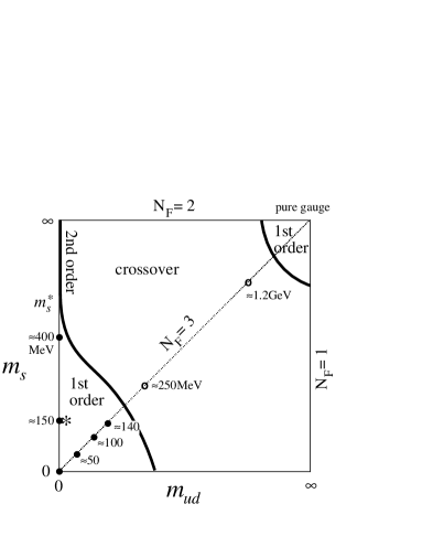
Figure 16: Phase diagram of $QCD$ according to Ref.[119]. First order phase transition is seen at solid circles and is not seen at blank circles. The star marks out the physical values of quark masses.

The bend of the second order phase transition line separating the region with first order phase transition and the region with no phase transition reflects a recent finding [137] that the shape of this line near the tricritical point $m_{s}=m_{s}^{*},m_{q}\equiv m_{u}=m_{d}=0$, where $m_{s}^{*}$ is the smallest value of the strange quark mass where we still have a second order phase transition in a theory with 2 massless quarks is

$$m_{s}^{*}-m_{s}\ \sim\ m_{q}^{5/2}$$ (5.24)

What is very surprising is the large value of $m_{s}^{*}\approx 450\ {\rm MeV}$ as measured in Ref.[119]. If they are right, the point corresponding to our physical world lies well inside the first order phase transition region in which case the first order phase transition should be of strong variety which contradicts Ref.[117] and also the theoretical arguments above.

Again, we do not know what of these two measurements is more correct. Possibly, intrinsic lattice artifacts are more dangerous when an algorithm with Wilson fermions is used [137, 138], but I do not have my own opinion on this point. To resolve the controversy, it would make sense, first, as was already mentioned, to test lattice methods on a two–dimensional playground and, second, to perform a quantitative comparison of the temperature dependence of the quark condensate as measured on lattices with the theoretical curve in Fig.14. Such a comparison has not been done so far.

To summarize, at the current level of understanding, the picture where the hadron gas goes over to quark-gluon plasma and other way round without any phase transition looks more probable. We have instead a sharp crossover in a narrow temperature range which is similar in properties to second-order phase transition (the “phase crossover” if you will).

5.4 Instantons and percolation.

In the discussion of the properties of the system at the vicinity of phase transition in this chapter, we relied so far on the fact that chiral symmetry is broken at zero temperature. It is an experimental fact in real $QCD$, but it is important to understand from pure theoretical premises why it is broken and what is the mechanism of its restoration at higher temperatures.

A completely satisfactory answer to this question has not yet been obtained. The problem is that $QCD$ at zero temperature is a theory with strong coupling and it is very difficult (may be impossible) to study the structure of $QCD$ vacuum state analytically from the first principles. However, a rather appealing qualitative physical picture exists [8, 139] which is based on the model of instanton-antiinstanton liquid and on the analogy with the so called percolation phase transition in doped superconductors [51].

The starting point is the Banks and Casher relation (4.8). As we have seen, nonzero quark condensate means nonzero spectral density of the Euclidean Dirac operator at $\lambda=0$ and that implies the presence of rather small characteristic eigenvalues

$$\lambda\sim 1/(\Sigma V)\ll\lambda_{\rm free}\sim 1/L$$ (5.25)

in the spectrum. The question is what is the physical reason for these small eigenvalues to appear.

As far as we know, the first pioneer paper where a mechanism for generating small eigenvalues was proposed is Ref.[140] where small eigenvalues appeared as zero modes of monopole-like gauge field configurations. The disadvantage of this model is that the monopole configurations are static whereas it is natural to expect that characteristic gauge fields contributing to the Euclidean path integral at $T=0$ are more or less symmetric in all four directions with no particular axis being singled out. The model of instanton-antiinstanton liquid formulated in [141, 142] and developed later in [143] is much better in this respect. We refer the reader to a recent comprehensive review [139] for details and just elucidate here main physical point of the reasoning.

The basic assumption of the model is that a characteristic gauge field contributing in $QCD$ path integral is a medium of instantons and instantons as shown in Fig.17. It is not a “gas” of Callan, Dashen, and Gross [144] because the interaction between instantons and antiinstantons bringing about a short-range correlations between instanton positions and orientations cannot be neglected. A “liquid” is a more proper term [141].

Figure 17: Instanton-antiinstanton liquid.

Each individual instanton and antiinstanton involves a fermion zero mode [145]. Assuming the constant density of quasi-particles $\propto\mu_{hadr}^{4}$, the total number of zero modes in the Euclidean volume $V$ is $N\ =\ N_{I}+N_{A}\ \sim\ V\mu_{hadr}^{4}$. However, these are not exact zero modes. They are shifted from zero due to interaction between instantons and antiinstantons. In other words, individual instanton and antiinstanton zero modes $\psi^{(0)}_{I,A}(x)$ are not eigenfunctions of the full Dirac operator $\not\!\!{\cal D}\ =\ \gamma_{\mu}(\partial_{\mu}-iA_{\mu}^{\rm IA\ liquid})$, where

$$A_{\mu}^{\rm IA\ liquid}(x)\ =\ \sum_{i=1}^{N_{I}}A_{\mu}^{I}(x-x_{i})\ +\ \sum_{j=1}^{N_{A}}A_{\mu}^{A}(x-x_{j})\$$ (5.26)

If choosing $\psi_{I}^{(0)}(x-x_{i})$ and $\psi_{A}^{(0)}(x-x_{j})$ as a basis in the Hilbert space, the Dirac operator presents a matrix with off–diagonal elements

$$[\not\!\!{\cal D}]_{ji}\ \sim\ \int d^{4}x\ \psi_{A}^{\dagger(0)}(x-x_{j})\not\!\!{\cal D}\psi_{I}^{(0)}(x-x_{i})$$

$$[\not\!\!{\cal D}]_{ij}\ \sim\ \int d^{4}x\ \psi_{I}^{\dagger(0)}(x-x_{i})\not\!\!{\cal D}\psi_{A}^{(0)}(x-x_{j})$$ (5.27)

Diagonalizing this matrix gives $N$ eigenvalues which are not zero anymore, but are spread over the characteristic range $\Delta\lambda\sim\mu_{hadr}$. Assuming a uniform spread, the volume density of quasi-zero modes is $\rho(0)\sim N/(V\Delta\lambda)\sim\mu_{hadr}^{3}$. Due to Eq.(4.8), a nonzero quark condensate appears.

This picture is rather similar to what happens in a doped semiconductor with high enough doping. When a characteristic distance between individual atoms of the admixture is not large, the wave functions of outer electrons of these atoms overlap, and the electrons can jump from site to site. If the set of atoms of admixture with a noticeable overlap of wave functions forms a connected network in the space, the electrons can travel through this network at large distances and the specimen is a conductor. Note that it is not a standard metal mechanism of conductivity when the medium is a crystal, has the long- range order, and the electron wave functions are periodic Bloch waves. Here the distribution of the dope whose electrons are responsible for conductivity is stochastic and wave functions are complicated. The essential is that they are delocalized.

Thus one can say that the vacuum of $QCD$ is the “conductor” in a certain sense. For sure, there is no conductivity of anything in usual Minkowski space-time. Only the Euclidean vacuum functional has “conducting” properties. In principle, one can introduce formally the fifth time and write an analog of Kubo formula for conductivity in $QCD$, but the physical meaning of this “conductivity” is not clear. It is sufficient to say that, in a characteristic Euclidean gauge field background, the eigenfunctions of Dirac operator corresponding to small eigenvalues are delocalized. It would be interesting to check the latter statement explicitly for the lattice vacuum configurations or in the instanton model framework. Instanton study of this question is now in progress [146].

What happens if we heat the system ? The effective coupling constant $g^{2}(T)$ decreases, the action of individual instantons $S=8\pi^{2}/g^{2}(T)$ increases, and the density of quasi-particles $\propto\exp\{-S\}$ decreases. Correspondingly, the characteristic value of off-diagonal matrix elements (5.27) in Dirac operator decreases. Note also that the overlap integrals (5.27) decrease as the temperature increases even if the distance between instanton and antiinstanton is not changed. The matter is that the individual fermion zero modes of thermal instantons [147] fall down exponentially $\sim\exp\{-\pi Tr\}$ at large spatial distances, not just as a power $\sim 1/r^{3}$ as is the case at $T=0$. Both effects lead to suppression of overlap matrix elements at finite $T$. (Concrete numerical calculations [64, 139] show that the second effect is more important in the temperature region $T\sim 200$ MeV. Speaking of the instanton density, it falls down only by a factor 2 in this region. That means, in particular, that the value of the gluon condensate $<(\alpha_{s}/\pi)G^{2}>_{T}$ at the critical temperature is only twice as small as at zero temperature, and the gluon condensate is far from being melted down. This is another manifestation of the fact that the gluon condensate is not an order parameter of the chiral restoration phase transition. Neither it is an order parameter of the deconfinement phase transition in pure Yang–Mills theory.)

Let us look first at our doped semiconductor when we decrease the density of admixture. Below some critical density, the set of atoms with essential overlapping of wave functions does not form a connected network in 3-dimensional space anymore. The electrons can no longer travel far through this network, wave functions become localized, and the conductivity drastically falls down. This is called the percolation phase transition (see [51] for detailed discussion).

Likewise, there is a critical temperature in $QCD$ above which instantons and antiinstantons do not form anymore a connected cluster with an essential overlap of individual fermion zero modes (what overlap is “essential” and what is not is a numerical question. For condensed matter systems, computer estimates for the critical admixture density were performed long time ago. Corresponding calculations in thermal $QCD$ have been done only recently [64]). At high temperatures, few remaining quasi-particles tend to form “instanton- antiinstanton molecules”. These molecules tend to be “polarized” in imaginary time direction (the overlap integrals and, correspondingly, the “binding energy” for a molecule polarized along imaginary time axis is larger as the zero modes involve an exponential suppression factor only in spatial, but not in Euclidean time direction).

A characteristic Euclidean path integral configuration at high temperature (here “high” means just several hundred MeV) is drawn schematically in Fig.18. In this picture, the individual zero modes are not spread out uniformly in the range $\Delta\lambda\sim\mu_{hadr}$ after diagonalization, as was the case at zero temperature where instantons and antiinstantons formed an infinite cluster, but are just shifted by the value $\sim\mu_{hadr}$ due to interaction in individual molecules. Small eigenvalues in the spectrum of Dirac operator are absent and the fermion condensate is zero.

Figure 18: Gas of instanton-antiinstanton molecules (high $T$).

It is worthwhile to emphasize once more that this scenario of percolation phase transition leading to the molecular high-temperature phase is expected to hold only at $N_{f}\geq 2$. For $N_{f}=1$ with arbitrary small but nonzero fermion mass, molecules are effectively ionized even at very high temperatures and the “medium” presents a very dilute instanton-antiinstanton gas — the instanton density involves a product of two small factors: $\exp\{-8\pi^{2}/g^{2}(T)\}$ and the fermion mass $m$. Differentiating ${\rm log}Z$ over $m$ and sending $m$ to zero, one obtains a small but nonzero quark condensate [5, 115]. Cf. the analogous situation in the Schwinger model [40].

5.5 Disoriented chiral condensate.

When we talked in previous sections about “experimental” tests of theoretical predictions, we meant numerical lattice experiment. However, speaking of the particular problem of the phase transition in $QCD$ associated with chiral symmetry restoration, an intriguing possibility exists that a direct experimental evidence for such a transition can be obtained at the high-energy heavy ion collider RHIC which is now under construction.

After a head-on collision of two energetic heavy nuclei, a high temperature hadron “soup” is created. We do not call this soup the quark-gluon plasma because, even at RHIC energies, the temperature $T_{\rm RHIC}\sim 0.5$ GeV [3] would not be high enough to provide a sufficient smallness of the effective coupling $g^{2}(T)$ and to make the perturbation theory over this parameter meaningful. (As will be discussed in details in Chapter 6, a proper normalization point for the coupling constant is probably $2\pi T$ rather than $T$. Still perturbative corrections to the physical quantities like the free energy density appear to be rather large at $T\sim.5$ GeV, and the perturbative series does not display a sign of convergence.) What is important, however, is that, at RHIC energies, the temperature of the soup would be well above the estimate (5.18) for the phase transition temperature. The high-temperature state created in heavy nuclei collision would exist for a very short time, after which it expands, cools down and decays eventually into mesons.

Let us look in more details at the cooling stage. At high temperature, the fermion condensate is zero. Below phase transition, it is formed and breaks spontaneously chiral symmetry. This breaking means that the vacuum state is not invariant under the chiral transformations (4.2) and a direction in isotopic space is distinguished. What particular direction — is a matter of chance. This direction is specified by the condensate matrix

$$\Sigma_{ff^{\prime}}=<\bar{q}_{Lf}q_{Rf^{\prime}}>$$ (5.28)

For simplicity, we have assumed up to now that the condensate matrix is diagonal $\Sigma_{ff^{\prime}}=-\frac{\Sigma}{2}\delta_{ff^{\prime}}$. But any unitary matrix can be substituted for $\delta_{ff^{\prime}}$ (of course, it can be brought back in the form $\delta_{ff^{\prime}}$ by a chiral transformation ). In different regions of space, cooling occurs independently and flavor directions of condensate are not correlated. As a result, domains with different directions of condensate shown in Fig.19 are formed (cf. cooling down of a ferromagnetic below the Curie point).

Figure 19: Domains of disoriented chiral condensate in cooling hadron soup.

In our world, we do not observe any domains, however. The direction of the condensate in all spatial points is identical. This is a consequence of the fact that $u$- and $d$- quarks have nonzero masses which break chiral symmetry explicitly, the vacuum energy involves a term

$$E_{vac}\sim{\rm Tr}\{{\cal M}^{\dagger}\Sigma\}+{\rm c.c.}$$ (5.29)

and the only true vacuum state is (4.5) (in the basis where the quark mass matrix ${\cal M}$ is diagonal).

However, the masses of $u$- and $d$- quarks are rather small and one can expect that the domains with “wrong” direction of the condensate are sufficiently developed during the cooling stage before they eventually decay into true vacuum (4.5) with emission of pions.

This is a crucial assumption. A theoretic estimate of the characteristic size of domains they reach before decaying is very difficult and there is no unique opinion on this question in the literature. But if this assumption is true, we can expect to observe a very beautiful effect [149, 123] (for a recent review, see [137]). From the true vacuum viewpoint, a domain with disoriented $\Sigma_{ff^{\prime}}$ is a classical object — kind of a “soliton” (quotation marks are put here because it is not stable) presenting a coherent superposition of many pions. The mass of this quasi-soliton is much larger than the pion mass. The existence of such multi- pion coherent states was discussed long ago in pioneer papers [150] but not in relation with thermal phase transition.

Eventually, these objects decay into pions. Some of the latter are neutral and some are charged. As all isotopic orientations of the condensate in the domains are equally probable, the average fractions of $\pi^{0}$, $\pi^{+}$, and $\pi^{-}$ are equal: $<f_{\pi^{0}}>=<f_{\pi^{\pm}}>=\frac{1}{3}$ as is also the case for incoherent production of pions in, say, $pp$ collisions where no thermalized high-$T$ hadron soup is created.

But the distribution $P(f)$ over the fraction of, say, neutral pions is quite different in the case of incoherent and coherent production. In incoherent case, $P(f)$ is a very narrow Poissonic distribution with the central value $<f_{\pi^{0}}>=1/3$. The events with $f_{\pi^{0}}=0$ or with $f_{\pi^{0}}=1$ are highly unprobable: $P(0)\sim P(1)\sim\exp\{-CN\}$ where $N\gg 1$ is the total number of pions produced.

For coherent production, the picture is quite different. $\Sigma_{ff^{\prime}}$ is proportional to a $SU(2)$ matrix. Factorizing over $U(1)$, one can define a unit vector in isotopic space $\in S^{2}$. The fraction of $\pi^{0}$ produced would be just $f=\cos^{2}\theta$ where $\theta$ is a polar angle on $S^{2}$. The probability to have a particular polar angle $\theta$ normalized in the interval $0\leq\theta\leq\pi/2$ [ the angles $\theta>\pi/2$ do not bring about anything new as $f(\pi-\theta)=f(\theta)$ ] is $P(\theta)=\sin\theta$. After an elementary transformation, we get a normalized probability in terms of $f$:

$$P(f)df=\frac{df}{2\sqrt{f}}$$ (5.30)

As earlier, $<f>=1/3$, but the distribution in $f$ is now wide and the values $f=0$ and $f=1$ are quite probable.

Thus a hope exists that, in experiments with heavy ion collisions at RHIC, wild fluctuations in the fractions of neutral and charged pions would be observed. That would be a direct experimental indication that a quasi-phase-transition occurs where domains of disoriented chiral condensate of noticeable size are developed in a cooling stage. One can recall in this respect mysterious Centauro events with anomalously large fraction of neutral or of charged particles observed in cosmic ray experiments [151]. Cosmic ray experiment is not a heavy ion collision experiment and there are no strong theoretical reasons to expect the formation of hot hadron matter there (see, however, [149]), but who knows, may be that still was the first experimental observation of the $QCD$ phase transition ?

6 Quark–gluon plasma.

The last chapter of the review is devoted to the properties of high–temperature phase, the quark–gluon plasma. It is a very rich and interesting physical system which attracted lately a considerable attention of theorists. The number of the papers in SLAC archive involving the words “quark– gluon plasma” in the title exceeds seven hundred (not yet exceeds right now when I write it, but will certainly pass this mark by the time you read it). Thereby, this chapter is longer than others and still many issues were left undiscussed. In particular, we will touch only superficially a fascinating, but technical subject of effective lagrangian of soft modes and of nonabelian Vlasov equations. Instead, we will discuss at some length different physical phenomena which are specific for QGP with an emphasize on the problem of physical observability of various characteristics of QGP discussed in the literature.

6.1 Static Properties of $QGP$: a bird eye’s view.

We start with discussing static (thermodynamic) characteristics of QGP and find it useful to do it in two “rounds”. In this section, we describe gross physical features of the system and go down to details in the next one.

Thermodynamics

The basic thermodynamic characteristic of a finite $T$ system is its free energy. The lowest order results are derived exactly in the same way as for free pion gas (see Sect. 4.2). We have for a pure gluon system

$$\frac{F^{g}}{V}=2(N_{c}^{2}-1)T\int\frac{d^{3}p}{(2\pi)^{3}}\ln\left[1-e^{-\beta|{\bf p}|}\right]=-\frac{\pi^{2}T^{4}}{45}(N_{c}^{2}-1)$$ (6.1)

where $2(N_{c}^{2}-1)$ is the number of degrees of freedom of the gluon field (the factor 2 comes due to two polarizations). This is nothing else as the Stefan–Boltzmann formula multiplied by the color factor $N_{c}^{2}-1$. The quark contribution is obtained quite similarly. Taking the Pauli principle into account, we have instead of Eq.(4.20)

$$F^{q}=-T\ln Z=-T\ln\left[\prod_{\bf p}\left(1+e^{-\beta n|{\bf p}|}\right)^{4N_{c}N_{f}}\right]$$ (6.2)

where $4N_{c}N_{f}$ is the number of degrees of freedom. Trading the sum for the integral, we obtain

$$\frac{F^{q}}{V}\ =\ -4N_{c}N_{f}T\int\frac{d^{3}p}{(2\pi)^{3}}\ln\left[1+e^{-\beta|{\bf p}|}\right]\ =\ -\frac{7\pi^{2}T^{4}}{180}N_{c}N_{f}$$ (6.3)

Notice that in our world with $N_{c}=N_{f}=3$, the lowest order quark contribution to the free energy is roughly 2 times larger than the gluon one.

All other thermodynamic quantities of interest can be derived from the free energy by standard thermodynamic relations. For example, the pressure just coincides with the free energy with the sign reversed. The energy density is

$$E=F-T\frac{\partial F}{\partial T}$$ (6.4)

For massless particles in the lowest order the relation

$$E=3P=-3F$$ (6.5)

holds.

Debye screening.

Consider the gluon polarization operator in $QGP$ with account of thermal loop corrections. It is transverse, $k_{\mu}\Pi_{\mu\nu}(k)=0$. At zero temperature, transversality and Lorentz-invariance dictate the form $\Pi_{\mu\nu}(k)=\Pi(k^{2})(g_{\mu\nu}-k_{\mu}k_{\nu}/k^{2})$. At finite $T$, Lorentz-invariance is lost and the polarization operator presents a combination of two different (transverse and longitudinal) tensor structures. Generally, one can write

$$\Pi_{00}=\Pi_{l}(\omega,|{\bf k}|)$$

$$\Pi_{i0}=\frac{k_{i}\omega}{{\bf k}^{2}}\Pi_{l}(\omega,|{\bf k}|)$$

$$\Pi_{ij}=-\Pi_{t}(\omega,|{\bf k}|)(\delta_{ij}-k_{i}k_{j}/{\bf k}^{2})+\frac{\omega^{2}}{{\bf k}^{2}}\frac{k_{i}k_{j}}{{\bf k}^{2}}\Pi_{l}(\omega,|{\bf k}|)$$ (6.6)

Consider first the longitudinal part of the polarization operator in the kinematic region where $\omega$ is set to zero in the first place after which $k\equiv|{\bf k}|$ is also sent to zero. By the reasons which will be shortly seen, we denote this quantity $m_{D}^{2}$:

$$m_{D}^{2}=\lim_{k\to 0}\Pi_{l}(0,k)$$ (6.7)

To understand the physical meaning of this quantity, consider the correlator

$$<A_{0}^{a}({\bf x})A_{0}^{b}(0)>\sim\delta^{ab}\int\frac{d{\bf k}}{{\bf k}^{2}+m_{D}^{2}}e^{i{\bf k}{\bf x}}\propto e^{-m_{D}|{\bf x}|}$$ (6.8)

Thus $m_{D}$ coincides with the inverse screening length of chromoelectric potential $A_{0}$.

There is a clear analog with the usual plasma. A static electric charge immersed in the plasma is screened by the cloud of ions and electrons so that the potential falls down exponentially $\propto\exp\{-r/r_{D}\}$ where the Debye radius $r_{D}$ in an ordinary nonrelativistic plasma is given by the expression (see e.g. [22])

$$r_{D}^{-2}=\frac{4\pi ne^{2}}{T}+\frac{4\pi n(Ze)^{2}}{T}$$ (6.9)

where $n$ is the electron and ion density, $Z$ is the ion charge (so that the second term describes the ion contribution), and, to avoid unnecessary complications, we assumed that the electron and ion components of the plasma have the same temperature $T$ Calculating the one-loop thermal contribution to the gluon polarization operator (see Fig.20), one can easily obtain an analogous formula for $QGP$:

$$m_{D}^{2}=r_{D}^{-2}=\frac{g^{2}T^{2}}{3}\left(N_{c}+\frac{N_{f}}{2}\right)$$ (6.10)

where the first term describes the screening due to thermal gluons and the second term — the screening due to thermal quarks. The result (6.10) was first obtained by Shuryak [152]. It has the same structure as (6.9) (Note that the density of particles in ultrarelativistic plasma is expressed via the temperature, $n\propto T^{3}$). It is worth mentioning that the Debye screening is essentially a classical effect and not only quarks but also gluons induce screening rather than antiscreening. That should be confronted with the famous antiscreening of the charge in Yang-Mills theory at zero temperature due to quantum effects.

1.333

Figure 20: Gluon polarization operator in one loop.

In $QED$, the correlator $<A_{0}({\bf x})A_{0}(0)>_{T}$ is a gauge invariant object and also the notion of charge screening is unambiguous and well defined — there are classical electric charges and one can measure the potential of such a charge immersed in plasma by standard classical devices. Not so in QCD. We do not have at our disposal classical color charges due to confinement and the experiment of measuring the chromoelectric field of a test color charge cannot be carried out even in principle. Also the gluon polarization operator which enters the definition (6.8) of a Debye screening mass is generally speaking gauge-dependent. Thus a question of whether the Debye screening mass is a physical notion in a nonabelian theory is fully legitimate.

The answer to this question is positive. But with reservations.

Note first of all that though the gluon polarization operator is generally gauge-dependent, the Debye screening mass defined in (6.7) does not depend on the gauge in the leading order (we shall discuss also nonleading corrections in the next section). That suggests that the result (6.10) has an invariant physical meaning.

Indeed, one can consider a gauge-invariant correlator

$$C({\bf x})=<P({\bf x})P^{*}(0)>_{T}$$ (6.11)

where

$$P({\bf x})=\frac{1}{N_{c}}{\rm Tr}\exp\left\{i\int_{0}^{\beta}A_{0}({\bf x},\tau)d\tau\right\}$$ (6.12)

is the Polyakov line [both the Polyakov line and the correlator (6.11) were discussed at length in Chapter 3]. If $r=|{\bf x}|$ is not too large (the exact meaning of this will be specified later), the connected part of the correlator $C_{c}(r)=C(r)-C(\infty)$ (as was explained in Chapter 3, $C(\infty)$ is a nonzero constant) has an exponential behavior

$$C_{c}(r)\ \propto\ [G_{00}(r)]^{2}\ \propto\ \frac{1}{r^{2}}\exp\{-2m_{D}r\}$$ (6.13)

The correlator (6.11) can be attributed a physical meaning. $-T\ln C(r)$ coincides with the change of free energy of the system when putting there a pair of heavy quark and antiquark at distance $r$, the averaging over color spin orientations being assumed [35].

Also we shall see in the next section that the perturbative corrections $\sim g^{3}T^{4}$ to a perfectly well defined and physical quantity — the free energy — depend directly on the value of $m_{D}$.

Thus the notion of Debye screening mass in $QGP$ is physical, though, unfortunately, not to the same extent as it is in the usual plasma. The correlator (6.11) with the correlation length of fractions of a fermi cannot be directly measured even in a gedanken laboratory experiment — at least, we cannot contemplate such an experiment. But it can be measured in lattice numerical experiments which is almost as good. We shall see later that a number of other characteristics of $QGP$ have a similar semi-physical status.

Magnetic screening.

Debye mass describes the screening of static electric fields. In abelian plasma, magnetic fields are not screened whatsoever. Such a screening could be provided by magnetic monopoles, but they are not abundant in Nature. The absence of monopoles is technically related to one of the Maxwell equations $\partial_{i}B_{i}=0$. In the nonabelian case, the corresponding equation reads ${\cal D}_{i}B_{i}=0$ where $\cal D$ is a covariant derivative. Thus gluon field configurations with local color magnetic charge density $\rho_{m}\sim\partial_{i}B_{i}$ (with usual derivative) are admissible. The presence of such configurations in the gluon heat bath results in screening of chromomagnetic fields.

Let us see how it comes out in a perturbative calculation. Consider the one-loop graph in Fig.20a which contributes to the polarization operator of the spatial components of the gluon field $\Pi_{ij}(0,{\bf k})\propto\Pi_{t}(0,k)$. At high temperatures, it suffices to take into account only the lowest Matsubara frequency (with $\omega=0$) in gluon propagators. We have

$$\Pi_{t}(0,k)\sim g^{2}k^{2}T\int\frac{d^{3}p}{{\bf p}^{2}({\bf p}-{\bf k})^{2}}\sim g^{2}Tk$$ (6.14)

The numerical coefficient can be explicitly calculated, but it depends on the gauge and makes as such a little sense. The loop integral is determined by the low momentum region $|{\bf p}|_{char}\sim k\ll T$ (as we are interested in the large distance behavior of the gluon Green’s function, we keep $k$ small). Note that the Feynman integral for $\Pi_{l}(0,k)$ has a completely different behavior being saturated (in the leading order) by the loop momenta $|{\bf p}|\sim T$ — it is a so called hard thermal loop.

The transverse part of the gluon Green’s function is

$$G_{t}(0,k)\sim\frac{1}{{\bf k}^{2}+\Pi_{t}(0,k)}$$ (6.15)

We see that at $k\sim g^{2}T$ the one-loop contribution to the polarization operator is of the same order as the tree term $k^{2}$. One can estimate a two-loop contribution to $\Pi_{t}(0,k)$ which is of order $(g^{2}T)^{2}$. The factor $T^{2}$ here comes from two loops (we use the rule (2.7) and take into account only the contribution of the lowest Matsubara frequency in each loop). Similarly, a three-loop contribution to $\Pi_{t}(0,k)$ is of order $(g^{2}T)^{3}/k$, a four-loop contribution is of order $(g^{2}T)^{4}/k^{2}$ etc. (The growing powers of $k$ in the denominator are provided by infrared 3-dimensional loop integrals. Infrared integrals may also provide for a logarithmic singularity in external momentum $k$ in the two- loop and higher loop contributions, but weak logarithmic factors are of no concern for us here). At $k\sim g^{2}T$, all contributions are of the same order and the perturbation theory breaks down [39].

There is an alternative way to see it. Let us write down the expression for the partition function of the pure glue system at finite temperature:

$$Z=\int\prod dA^{a}_{\mu}({\bf x},\tau)\exp\left\{-\frac{1}{4g^{2}}\int_{0}^{\beta}d\tau\int d^{3}x(F^{a}_{\mu\nu})^{2}\right\}$$ (6.16)

When $T$ is large and $\beta$ small, the Euclidean time dependence of the fields may be disregarded. Also the effects due to $A_{0}({\bf x},\tau)$ can be disregarded — time components of the gluon field acquire the large mass $m_{D}\sim gT\gg g^{2}T$ and decouple. We are left with the expression

$$Z=\int\prod dA^{a}_{i}({\bf x})\exp\left\{-\frac{1}{4g^{2}T}\int d^{3}x(F^{a}_{ij})^{2}\right\}$$ (6.17)

A theory with quarks is also reduced to (6.17) in this limit — the fermions have high Matsubara frequencies $\sim T$ and decouple. The partition function (6.17) describes a nonlinear 3D theory with the dimensional coupling constant $g_{3}^{2}\sim g^{2}T$ . No perturbative calculations in this theory are possible.

In $QED$, there is no magnetic screening (and the effective 3-dimensional theory is trivial). Presumably, perturbative calculations in hot $QED$ can be carried out at any order, though this question is not absolutely clear.

What is the physical meaning of this nonabelian screening ? Can it actually be measured ?

The way we derived it, the magnetic screening shows up in the large distance behavior of the spatial gluon propagator $G_{t}(r)\propto\exp\{ik^{*}r\}$ where $k^{*}$ is the solution to the equation

$$k^{2}+\Pi_{t}(0,k)=0$$ (6.18)

There is no reason to expect that $k=0$ is a solution — the behavior of $\Pi_{t}(0,k)$ in the limit $k\to 0$ where the perturbation theory does not work is not known, but one can tentatively guess that it tends to a constant $\sim(g^{2}T)^{2}$ (As we have seen, $g^{2}T$ is the only relevant scale in this limit). If so, $k^{*}\sim ig^{2}T$ and $G_{t}(r)$ falls down exponentially $\propto\exp\{-Cg^{2}Tr\}$ at large distances. Hence the term “magnetic screening”.

Unfortunately, the gluon polarization operator is a gauge- dependent quantity and, would the God provide us with the exact expression for $\Pi_{t}(0,k)$ in any gauge, even He could not guarantee that the solution of the dispersive equation (6.18) would be gauge-independent .

What one can do, however, is to consider the correlator of chromomagnetic fields $C_{ab}({\bf x})\ =\ <{\bf B}^{a}({\bf x}){\bf B}^{b}(0)>_{T}$. This correlator also depends on the gauge in a nonabelian theory, but the gauge dependence amounts to rotation in color space: $C_{ab}({\bf x})\to\Omega_{a^{\prime}a}({\bf x})C^{a^{\prime}b^{\prime}}({\bf x})\Omega_{b^{\prime}b}(0)$ and cannot affect the exponential behavior of the propagator. This is the way the magnetic mass is usually measured on the lattices.

One can do even better considering gauge-invariant correlators, the simplest one is   $<G_{\mu\nu}^{2}({\bf x})G_{\mu\nu}^{2}(0)>_{T}$. Then the quantity

$$\mu=-\lim_{r\to\infty}\frac{1}{r}\ln<G_{\mu\nu}^{2}({\bf x})G_{\mu\nu}^{2}(0)>_{T}$$ (6.19)

provides an invariant definition of the magnetic screening mass. The indefinite article is crucial here. Choosing other gauge-invariant correlators, one would get other invariant definitions. For example (and this will be important in the following discussion), the true correlation length of the correlator of Polyakov loops (6.11) is also of order $(g^{2}T)^{-1}$. The asymptotics (6.13) is an intermediate one and holds only in the region

$$(gT)^{-1}\ll r\ll(g^{2}T)^{-1}$$ (6.20)

What was wrong with our previous derivation ? The matter is we took into account earlier only the thermal corrections to the gluon propagator and tacitly neglected corrections to the vertices. Ab accurate analysis [27] shows that this is justified in the range (6.20) but not beyond. An example of the graph providing the leading contribution in $<P({\bf x})P^{*}(0)>_{T}$ at $r\gg(g^{2}T)^{-1}$ is given in Fig.21.

2

Figure 21: Correlator of Polyakov loops at large distances. Wavy lines are electric gluons and dashed lines are magnetic gluons.

Thus the “experimental status” of the magnetic mass (6.19) and of other similar quantities is roughly the same and even better than for the Debye mass. The exponential behavior $\propto\exp\{-\mu r\}$ of the correlators is expected to hold at any large $r$ and the value $\mu$ can in principle be determined in lattice experiments with any desired accuracy. On the other hand, the Debye screening mass cannot be determined with an arbitrary accuracy due to the finite range (6.20) where the asymptotics (6.13) holds (being sophisticated enough, an invariant definition of Debye mass still can be suggested for $N_{c}\geq 3$ — see the discussion in the following section). And, as was also the case for the Debye mass, we cannot invent any laboratory experiment where the magnetic mass could be directly measured.

Speaking of the lattice experiment, it can be done and actually has been done very recently by the Bielefeld group. Electric and magnetic screening lengths were measured in the high temperature region up to $T\sim 10^{6}{\rm GeV}$. Preliminary data [155] show a slow falloff of the quantities $m_{D}/T$ and $\mu_{\rm magn}/T$ with temperature in a qualitative agreement with the expected behavior $m_{D}/T\sim g(T)$ and $\mu_{\rm magn}/T\sim g^{2}(T)$.

6.2 Static Properties of $QGP$: perturbative Corrections.

Debye mass.

To provide a smooth continuation of the discussion started at the end of the previous section, we consider first higher-loop effects in the Debye mass. Note first of all that the definition (6.7) is not suitable anymore. Higher-loop corrections $\Delta m_{D}\sim g^{2}T$ to the Debye mass as defined in Eq.(6.7) depend on the gauge [156]. A better way is to define the Debye mass as the solution of the dispersive equation $k^{2}+\Pi_{l}(0,k)=0$. In other words, we define [157]

$$m_{D}^{2}=\lim_{k^{2}\to-m_{D}^{2}}\Pi_{l}(0,k)$$ (6.21)

The longitudinal part of the gluon Green’s function

$$G_{l}(0,k)=\frac{1}{k^{2}+\Pi_{l}(0,k)}$$

has then the pole at $k=im_{D}$. Pole position has the “tendency” to remain gauge-invariant even though the Green’s function itself is not. We will see in the following section that there are cases when formal arguments displaying gauge-invariance of the pole position fail in higher orders of perturbation theory due to severe infrared singularities. Speaking of Debye mass as defined in Eq.(6.21), its gauge invariance can be shown in the order $\sim g^{2}T\ln(C/g)$, but the constant under the logarithm is not computable in perturbation theory in principle, and it is difficult to pose a question whether it is gauge–invariant or not. In the next-to-leading order, the (gauge-invariant) result is [157]

$$m_{D}\ =\ m_{D}^{(0)}+\frac{N_{c}g^{2}T}{4\pi}\ln(C/g)$$ (6.22)

with logarithmic accuracy. As was mentioned, the constant $C$ is not computable by perturbation theory. We see that the correction is non-analytic in coupling constant. The non-analyticity appears due to bad infrared behavior of the loop integrals — they involve a logarithmic infrared divergence and depend on the low momenta cutoff which is of order of magnetic mass scale $g^{2}T$. Thus we have

$$\Delta m_{D}^{2}\propto\int_{\mu_{mag}}^{m_{D}}\frac{dp}{p}=\ln{m_{D}\over\mu_{mag}}\sim\ln{1\over g}$$

The magnetic infrared cutoff is actually provided by higher- order graphs — the orders of perturbation theory are mixed up and a pure two-loop calculation is not self-consistent. As we have seen, $\mu_{mag}$ cannon be determined analytically which means that the correction $\sim g^{2}T$ without the logarithmic factor in the Debye mass cannot be determined analytically.

Also the correction $\sim g^{2}T$ cannot be “experimentally observed”. Really, we have seen that the invariant physical definition of $m_{D}$ refers to the correlator of Polyakov loops (6.11). The latter displays the exponential behavior (6.13) in the limited range (6.20). But that is tantamount to saying that the correction $\sim g^{2}T$ in the Debye mass cannot be determined from the correlator (6.11). To do this, one should probe the distances $r\gg(g^{2}T)^{-1}$ where the correlator has a completely different behavior being determined by the magnetic scale. The correction (6.22) is still observable, however, due to a logarithmic enhancement factor.

To be more precise, the correlator in the range (6.20) has the form [27]

$$C_{c}(r)\ =\ \frac{N_{c}^{2}-1}{8N_{c}^{2}}\frac{g^{4}}{(4\pi rT)^{2}}\exp\left\{-2m_{D}^{(0)}r-\frac{N_{c}g^{2}Tr}{4\pi}\ln(m_{D}^{(0)}r)\right\}$$ (6.23)

where $m_{D}^{(0)}$ is the lowest order Debye mass (6.10).

It is not just

$$C_{c}(r)\ \propto\ \exp\{-2m_{D}r\}$$ (6.24)

, with $m_{D}$ being defined in (6.22), by two reasons. First, at finite $r\ll(g^{2}T)^{-1}$, the infrared cutoff in the loop integrals is provided by $r^{-1}$ rather than $\mu_{mag}$ and we have

$$\ln\frac{1}{g}\sim\ln{m_{D}\over\mu_{mag}}\to\ln(m_{D}r)$$ (6.25)

Second, there are two kinds of graphs involving the corrections both in the gluon propagator and in the vertex (see Fig.22).

2

Figure 22: Correlator of Polyakov loops in next–to–leading order. Wavy lines are electric gluons with Debye mass (6.10) taken into account. Dashed lines are magnetic gluons.

The graph in Fig.22a would give the correction

$$\frac{C_{c}(r)}{C_{c}^{(0)}(r)}\ \sim\ 1-\frac{N_{c}g^{2}Tr}{2\pi}\ln(m_{D}r)$$ (6.26)

with logarithmic accuracy. It corresponds to Eq.(6.24) where the substitution (6.25) is made. The second graph also contributes in this order and gives a positive correction with a twice as small coefficient [27]. Exponentiating the one loop correction , we arrive at the result (6.23). Note that the Fourier image of the correlator (6.23) does not have a singularity at finite $k$ whatsoever. Thus the Debye mass pole in the gluon propagator does not show up as a pole in the gauge-invariant correlator of Polyakov loops. Thereby, the quantity (6.22) is not quite physical in spite of its gauge invariance.

But, anyway, in the theoretical limit $\ln[1/g(T)]\to\infty$, there is a narrow range of $r$ where the condition $r\ll(g^{2}T)^{-1}$ is fulfilled so that the intermediate asymptotic law (6.23) holds whereas the correction in the exponent $\propto gm_{D}^{(0)}r\ln(m_{D}r)$ is of order 1 and can in principle be singled out in numerical lattice experiment.

There are two interesting recent proposals to define Debye mass non-perturbatively in a gauge-invariant way [153]. The first one is to consider the correlator of imaginary parts of Polyakov lines in a complex representation. If we are interested in a pure Yang–Mills theory, an additional requirement for the representation to be invariant under the action of the center of the group $Z_{N}$ (such is, say, the decouplet representation in $SU(3)$) should be imposed. . The point is that $P^{*}_{10}-P_{10}$ is odd under Euclidean time reversion and cannot be coupled to only magnetic gluons. That means that the correlator

$$<P^{*}_{10}({\bf x})-P_{10}({\bf x}),\ \ P^{*}_{10}(0)-P_{10}(0)>_{T}$$ (6.27)

exhibits the Debye screening falloff even at arbitrary large $r$. In the intermediate region (6.20), the correlator (6.27) is described by the graph with exchange of 3 electric gluons and falls down as $\propto\exp\{-3m_{D}r\}$. At very large distances, the dominant graph corresponds to the exchange of one electric gluon which is odd under the time reversion + a cloud of light magnetic gluons which neutralize the color. Debye mass extracted from the exponential falloff of such a correlator at large distances has a gauge invariant meaning, but depends, generally speaking, on the choice of the representation (probably, not in the order $g^{2}T\ln(1/g)$). Also this definition does not work for $SU(2)$ where the Polyakov line is real in any representation.

Another suggestion was to study the behavior of large spatial Wilson loops in adjoint color representation. At large distances, the theory is effectively reduced to the 3- dimensional YM theory (6.17). Adjoint color charges in this theory are not confined but rather screened, and the Wilson loop exhibits the perimeter law behavior

$$W(C)\propto\exp\{-m^{*}\times{\rm perimeter}(C)\}$$ (6.28)

One can show that $m^{*}$ is of order $g^{2}\ln(1/g)T$ and coincides with a perturbative correction to the Debye mass in (6.22). The problem here is that $m^{*}$ has no trace of the lowest order contribution (6.10). Still, $m^{*}$ certainly has an invariant meaning and is as such an interesting quantity to study.

Free energy.

This is the most basic and physical quantity of all. May be this is the reason why perturbative corrections are known here with record precision.

2

Figure 23: Free energy in two loops.

The correction $\sim g^{2}T^{4}$ has been found by Shuryak [152]. To this end, one should calculate the two-loop graphs depicted in Fig.23. The behavior of Feynman integrals in this order is quite benign and no particular problem arises.

2

Figure 24: An infrared-divergent 3-loop graph in free energy.

However, starting from the three-loop level, the problems crop up. The contribution of the graph depicted in Fig.24 is infrared divergent:

$$\Delta F^{Fig.\ref{FQGP3}}\sim g^{4}T^{5}\int\frac{dk}{k^{2}}$$ (6.29)

That means that a pure 3-loop calculation is not self- consistent and, to get a finite answer, one has to resum a set of infrared-divergent graphs in all orders of perturbation theory. This is, however, not a hopeless problem, and it has been solved by Kapusta back in 1979 [158]. The leading infrared singularity is due to the so called “ring diagrams” depicted in Fig.25.

2

Figure 25: Ring diagrams. Grey circles stand for a set of one-loop graphs in Fig.20

The sum of the whole set of ring diagrams has the form

$$F^{ring}\sim T\int d^{3}k\left\{\ln\left[1+\frac{\Pi_{l}(0,k)}{k^{2}}\right]-\frac{\Pi_{l}(0,k)}{k^{2}}\right\}$$ (6.30)

The expansion of the integrand in ${\Pi_{l}(0,k)}/{k^{2}}$ restores the original infrared-divergent integrals. However, the whole integral is convergent being saturated by momenta of order $k\sim[\Pi_{l}(0,0)]^{1/2}\sim gT$. Neglecting the $k$-dependence in the polarization operator, we obtain

$$F_{3}\sim T\int d^{3}k\left[\ln\left(1+\frac{m_{D}^{2}}{k^{2}}\right)-\frac{m_{D}^{2}}{k^{2}}\right]\sim Tm_{D}^{3}\sim g^{3}T^{4}$$ (6.31)

We see that the correction is non-analytic in the coupling constant $\alpha_{s}$ which exactly reflects the fact that the individual graphs diverge and the orders of perturbation theory are mixed up. Note, however, that infrared divergences here are of comparatively benign variety — the integral depends on the scale $k^{char}\sim gT$ and we are far from the land of no return $k\sim g^{2}T$. That is why an analytic determination of the coefficient in (6.31) is possible.

The next correction has the order $\sim g^{4}T^{4}\ln(1/g)$. It comes from the same ring graphs of Fig.25 where now the term $\sim g^{2}Tk$ in $\Pi_{l}(0,k)$ should be taken into account. This correction was determined by Toimela [159].

Presently, the correction $\sim g^{4}T^{4}$ (without the logarithmic factor) [160] and the correction $\sim g^{5}T^{4}$ [161, 162] are known. This is the absolute limit beyond which no perturbative calculation is possible — similar ring graphs as in Fig.25 but with magnetic gluons would give the contribution $\propto T\mu_{mag}^{3}\sim g^{6}T^{4}$ in the free energy. And, as we have seen, $\mu_{mag}$ cannot be determined perturbatively.

Collecting all the terms, the following result is obtained [161, 162]

$$F=-\frac{8\pi^{2}T^{4}}{45}\left[F_{0}+F_{2}\frac{\alpha_{s}(\mu)}{\pi}+F_{3}\left(\frac{\alpha_{s}(\mu)}{\pi}\right)^{3/2}+\right.$$

$$\left.F_{4}\left(\frac{\alpha_{s}}{\pi}\right)^{2}+F_{5}\left(\frac{\alpha_{s}}{\pi}\right)^{5/2}+O(\alpha_{s}^{3}\ln\alpha_{s})\right]$$ (6.32)

where

$$F_{0}=1+\frac{21}{32}N_{f}$$ (6.33)

$$F_{2}=-\frac{15}{4}\left(1+\frac{5}{12}N_{f}\right)$$ (6.34)

$$F_{3}=30\left(1+\frac{N_{f}}{6}\right)^{3/2}$$ (6.35)

$$F_{4}=237.2+15.97N_{f}-0.413N_{f}^{2}+\frac{135}{2}\left(1+\frac{N_{f}}{6}\right)\ln\left[\frac{\alpha_{s}}{\pi}\left(1+\frac{N_{f}}{6}\right)\right]$$

$$-\frac{165}{8}\left(1+\frac{5}{12}N_{f}\right)\left(1-\frac{2}{33}N_{f}\right)\ln\frac{\mu}{2\pi T}$$ (6.36)

$$F_{5}=\left(1+\frac{N_{f}}{6}\right)^{1/2}\left[-799.2-21.96N_{f}-1.926N_{f}^{2}\right.$$

$$\left.+\frac{485}{2}\left(1+\frac{N_{f}}{6}\right)\left(1-\frac{2}{33}N_{f}\right)\ln\frac{\mu}{2\pi T}\right]$$ (6.37)

The expressions (6.33) - (6.2) are written for $N_{c}=3$. The coefficients like 237.2 are not a result of numerical integration but are expressed via certain special functions.

A nice feature of the result (6.2) is its renorm- invariance. The coefficients $F_{4}$ and $F_{5}$ involve a logarithmic $\mu$–dependence in such a way that the whole sum does not depend on the renormalization scale $\mu$.

Let us choose $\mu=2\pi T$ (this is a natural choice [99], $2\pi T$ being the lowest nonzero gluon Matsubara frequency ) and $N_{f}=3$. In that case, we have

$$F=F_{0}\left[1-0.9\alpha_{s}+3.3\alpha_{s}^{3/2}+(7.1+3.5\ln\alpha_{s})\alpha_{s}^{2}-20.8\alpha_{s}^{5/2}\right]$$ (6.38)

Note a large numerical coefficient at $\alpha_{s}^{5/2}$. It is rather troublesome because the correction $\sim\alpha_{s}^{5/2}$ overshoots all previous terms up to very high temperatures and, at temperatures which can be realistically ever reached at accelerators, makes the whole perturbative approach problematic.

Take $T\sim 0.5\ {\rm GeV}$ (as was mentioned earlier, this is the temperature one can hope to achieve at RHIC [3]). Then $2\pi T\sim 3\ {\rm GeV}$ and $\alpha_{s}\sim 0.2$. (We use a conservative estimate for $\alpha_{s}$ following from $\Upsilon$ physics [163]. Recent measurements at LEP favor even larger values.). The series (6.38) takes the form

$$F=F_{0}[1-.18+.3+.06-.37+\ldots]$$ (6.39)

which is rather unsatisfactory. We emphasize that the coefficient of $\alpha_{s}^{5/2}$ is rather trustworthy being obtained independently by two different groups.

The estimate (6.39) was obtained in the assumption $N_{f}=3$. In pure Yang-Mills theory, the behavior of perturbative series is even worse :

$$F=F_{0}\left[1-1.19\alpha_{s}+5.39\alpha_{s}^{3/2}+(16.20+6.84\ln\alpha_{s})\alpha_{s}^{2}-45.69\alpha_{s}^{5/2}\right]$$ (6.40)

which means that perturbation theory cannot be trusted at all at $\alpha_{s}$ $\ {}^{>}_{\sim}\ .15$. One could naively expect that deviations of real free energy density from Stephan–Boltzmann value would be considerable up to very large temperatures. Somewhat surprisingly, numerical lattice calculations show it is not the case. According to recent measurements in pure $SU(3)$ Yang–Mills theory [164], the free energy density at $T=5T_{c}$ constitutes 85% of the Stephan–Boltzmann value. This suggests that the coupling constant in this region is small. Indeed, the estimate for the coupling constant obtained in [164] from measurement of another lattice quantity, the spatial string tension, is $\alpha_{s}\approx.12$ at $T=5T_{c}$. If substituting it in the series (6.40), we find $F/F_{0}\approx.87$ in a perfect agreement with the data. Actually, the smallness of the coupling constant here is an “optical illusion”. When comparing the pure Yang– Mills theory with $QCD$ with quarks, one should compare the scale of perturbative corrections which is of order $\sim\alpha_{s}c_{V}$ in the pure Yang–Mills theory versus $\sim\alpha_{s}c_{F}$ in $QCD$. This scale is roughly the same in pure YM theory and in QCD for the same temperature (measured in units of string tension $\sigma$ or in units of $T_{c}$).

At lower temperatures, perturbation theory does not work and non-perturbative effects (associated with instantons) become important. The lattice values of the ratio $F/F_{0}$ rapidly decrease with temperature and are rather small at $T\sim T_{c}$.

The last remark is technical. The result (6.2) was obtained in Euclidean technique. There is a real time calculation which correctly reproduces the two-loop term $\sim g^{2}T^{4}$ in free energy [17], but nobody so far succeeded in calculating in this way the terms $\sim g^{3}T^{4}$ and higher. Certainly, real-time technique is not very suitable for calculation of static quantities, and one way to get the result is good enough, but, to my mind, it is an interesting methodical problem.

6.3 Collective excitations.

One of striking and distinct physical phenomena characteristic of usual plasma is a non-trivial dispersive behavior of electromagnetic waves. In contrast to the vacuum case where only transverse photons with the dispersive law $\omega=|{\bf k}|$ propagate, two different branches with different non-trivial dispersive laws $\omega_{\bot}(k)$ and $\omega_{\|}(k)$ appear in plasma. The value $\omega_{\bot}(0)=\omega_{\|}(0)=\omega_{pl}$ characterizes the eigenfrequency of spatially homogeneous charge density oscillations and is called the plasma frequency.

A similar phenomenon exists also in $QGP$. The spectrum of $QGP$ involves collective excitations with quantum number of quarks and gluons. Like in usual plasma, there are transverse and longitudinal branches of gluon collective excitations (alias, transverse and longitudinal plasmons) and their properties on the one-loop level are very similar to the properties of photon collective excitations in usual plasma. A novel feature is the appearance of non-trivial fermion collective excitations (plasminos). But, again, they are not specific for a nonabelian theory and appear also in ultrarelativistic $e^{+}e^{-}$ plasma (in the limit when the electron mass can be neglected compared to the temperature-induced gap in the electron spectrum $\propto eT$).

One-loop calculations.

The dispersive laws of quark and gluon collective excitations can be obtained via solution of a nonabelian analog of the Vlasov system involving the classical field equations in the medium and Boltzmann kinetic equation [165]. This way of derivation makes analogies with usual plasma (where the Vlasov system is a standard technique) the most transparent.

I will outline here another way of derivation which is more conventional and more easy to understand for a field theorist. This is actually the way the results were originally derived [166, 167] (Note, however, that analogous results for abelian ultrarelativistic plasma were first derived long time ago in Vlasov technique [168]).

Consider the gluon Green’s function in a thermal medium. As was mentioned in sect. 2, at $T\neq 0$, different kinds of Green’s function exist. To be precise, we are considering now the retarded Green’s function

$$\left[G_{\mu\nu}^{ab}(x)\right]^{R}\ =\ -i<\theta(t)[A_{\mu}^{a}(x),A_{\nu}^{b}(0)]>_{T}$$ (6.41)

which describes a response of the system on a small perturbation applied at $t=0$ at some later time $t>0$. As was discussed in details in Sect. 2.2, the Fourier image of (6.41) is free of singularities in the upper $\omega$ half–plane. The poles of $G^{R}_{\mu\nu}(\omega,{\bf k})$ correspond to eigenmodes of the system and exactly give us the desired spectrum of gluon collective excitations. The dispersive equation

$$\det\|[G^{R}_{\mu\nu}(\omega,k)]^{-1}\|=0$$ (6.42)

splits up in two:

$$\omega^{2}-k^{2}-\Pi_{t}(\omega,k)=0$$

$$k^{2}+\Pi_{l}(\omega,k)=0$$ (6.43)

with $\Pi_{l,t}(\omega,k)$ being defined in Eq.(6.1). The solutions to the equations (6.3) give two branches of the spectrum.

The explicit one-loop expressions for $\Pi_{l}(\omega,k)$ and $\Pi_{t}(\omega,k)$ obtained by the calculation of the graphs in Fig.20 in the limit $\omega,k\ll T$ are [166, 167]

$$\Pi_{l}(\omega,k)=3\omega_{pl}^{2}[1-F(\omega/k)]$$

$$\Pi_{t}(\omega,k)=\frac{3}{2}\omega_{pl}^{2}\left[\frac{\omega^{2}}{k^{2}}+\frac{k^{2}-\omega^{2}}{k^{2}}F(\omega/k)\right]$$ (6.44)

where

$$\omega_{pl}=\frac{gT}{3}\sqrt{N_{c}+\frac{N_{f}}{2}}$$ (6.45)

is the plasma frequency and

$$F(x)=\frac{x}{2}\ln\frac{x+1}{x-1}$$ (6.46)

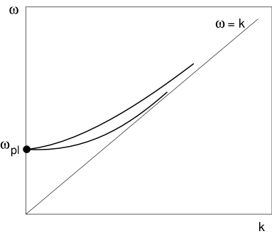
Figure 26: Plasmon spectrum in one loop.

The behavior of dispersive curves is schematically shown in Fig.26. At $k=0$, $\omega_{\bot}(0)=\omega_{\|}(0)=\omega_{pl}$. Then the two branches diverge:

$$\omega^{2}_{\bot}(k\ll gT)=\omega_{pl}^{2}+\frac{6}{5}k^{2}$$

$$\omega^{2}_{\|}(k\ll gT)=\omega_{pl}^{2}+\frac{3}{5}k^{2}$$ (6.47)

At $k\gg gT$ both branches tend to the vacuum dispersive law

$$\omega^{2}_{\bot}(k\gg gT)=k^{2}+\frac{3}{2}\omega_{pl}^{2}$$

$$\omega^{2}_{\|}(k\gg gT)=k^{2}\left[1+4\exp\left(-\frac{2k^{2}}{3\omega_{pl}^{2}}-2\right)\right]$$ (6.48)

We see that $\omega_{\|}(k)$ approaches the line $\omega=k$ exponentially fast.

The dispersive laws for quark collective excitations are obtained from a similar analysis of the quark Green’s function. One loop expression for the finite temperature contribution in the fermion polarization operator in the limit $\omega,k\ll T$ is

$$\Sigma(\omega,{\bf k})\ =\ \gamma^{0}\frac{\omega_{0}^{2}}{\omega}F(\omega/k)\ -\ \frac{\mbox{\boldmath$\gamma$}{\bf k}}{k}\frac{\omega_{0}^{2}}{k}[F(\omega/k)-1]$$ (6.49)

where $\omega_{0}$ is the plasmino frequency at zero momentum:

$$\omega_{0}^{2}=\frac{g^{2}T^{2}}{8}c_{F}$$ (6.50)

We see that the fermion polarization operator involves two tensor structures $\omega\gamma^{0}-{\bf k}\mbox{\boldmath$\gamma$}$ and $\omega\gamma^{0}+{\bf k}\mbox{\boldmath$\gamma$}$ which gives rise to two dispersive branches. We will call the branch corresponding to the Lorentz-invariant structure “transverse” and the branch corresponding to the structure $\omega\gamma^{0}+{\bf k}\mbox{\boldmath$\gamma$}$ — “longitudinal”. These terms may be misleading in the fermion case because, in contrast to the plasmons with photon or gluon quantum numbers, these branches are not associated with transverse and longitudinal field polarizations. Hence the quotation marks. But better names were not invented, and using the words “transverse” and “longitudinal” still makes a certain sense because the physical properties of “transverse” and “longitudinal” fermion branches are rather analogous to the physical properties of transverse and longitudinal gluon branches.

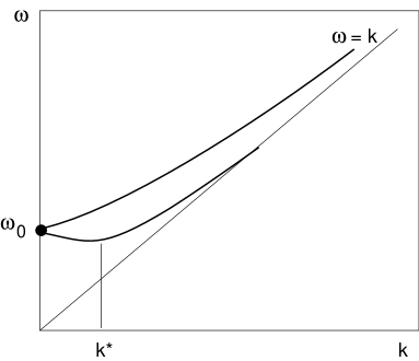
Figure 27: Plasmino spectrum in one loop.

The pattern of the quark spectrum is shown in Fig.27. It is similar to the gluon spectrum with one important distinction — at $k\sim 0$, $\omega_{\bot}(k)$ and $\omega_{\|}(k)$ involve linear terms of opposite sign:

$$\omega^{q}_{\bot}(k\ll gT)=\omega_{0}+\frac{k}{3}$$

$$\omega^{q}_{\|}(k\ll gT)=\omega_{0}-\frac{k}{3}$$ (6.51)

Thus $\omega^{q}_{\|}(k)$ first goes down and reaches minimum at some $k^{*}$. The group velocity of the longitudinal plasmino at this point is zero. At large $k$,

$$\omega_{\bot}^{q2}(k\gg gT)\ =\ k^{2}+2\omega_{0}^{2}$$ (6.52)

and $\omega_{\|}^{q}$ tends from above to the line $\omega=k$ exponentially fast.

Landau Damping.

The quoted one-loop results for the dispersive laws of transverse plasmons and plasminos are gauge-invariant and stable with respect to higher-order corrections. The latter is not true, however, for longitudinal excitation branches [169, 170]. We have seen that $\omega_{\|}^{1\ loop}(k)$ tends to the line $\omega=k$ exponentially fast at $k\gg gT$. This can be easily seen from the analysis of the dispersive equations for longitudinal branches which, in the limit $k\gg gT$, have the form

$$\omega_{\|}+k\sim\frac{g^{2}T^{2}}{k}\ln\frac{k}{\omega_{\|}-k}$$ (6.53)

At $k\gg gT$, the solution exists when the logarithm is large and $\omega_{\|}-k$ is exponentially small. The logarithmic factor in Eq.(6.53) comes from the angular integral

$$\sim\int\frac{d\theta}{\omega-k\cos\theta}$$ (6.54)

which diverges at $\omega=k$. This collinear divergence appears due to masslessness of quarks and gluons in the loop depicted in Fig.20. But quarks and gluons in $QGP$ are not massless — their dispersive law acquires the gap $\sim gT$ due to temperature effects. An accurate calculation requires substituting in the loops the dressed propagators. As a result, the logarithmic divergence in the integral (6.54) is cut off and the logarithmic factor in Eq.(6.53) is modified:

$$\ln\frac{k}{\omega-k}\to\frac{1}{2}\ln\frac{k^{2}}{(\omega-k)^{2}+Cg^{2}T^{2}}$$ (6.55)

Dressing of propagators amounts to going beyond one-loop approximation. Strictly speaking, to be self-consistent, one should also take into account one-loop thermal corrections to the vertices (this procedure is known as resummation of hard thermal loops [171]), but in this particular case these corrections do not play an important role. What is important is the cutoff of the logarithmic collinear singularity due to effective temperature-induced masses.

Substituting (6.55) in (6.53), we see that the new dispersive equation does not at all have solutions with real $\omega$ for large enough $k$. This fact can be given a natural physical explanation. When $k$ is small compared to $gT$, there is no logarithmic factor in the dispersive equation, the modification (6.55) is irrelevant, and the dispersive law of longitudinal modes does not deviate from the one-loop result. Then the logarithm appears, the modification (6.55) starts playing a role, and, at some $k^{**}\sim gT$, the longitudinal dispersive curve crosses the line $\omega=k$. At this point the longitudinal polarization operator acquires the imaginary part due to Landau damping.

In usual plasma, Landau damping is the process when propagating electromagnetic waves are “absorbed” by the electrons moving in plasma. In the language of quantum field theory, it is a $2\to 1$ process

$$\gamma^{*}+e\to e$$ (6.56)

In real time technique, that corresponds to a contribution to the imaginary part of the polarization operator so that both internal electron lines in the loop are placed on mass shell. At $T=0$ the standard Cutkosky rules imply positive energies of all particles in the direct channel, and the imaginary part appears only due to the decay $\gamma^{*}\to e^{+}+e^{-}$. At $T\neq 0$, Cutkosky rules are modified and both signs for energy are admissible. Physically, that corresponds to the presence of real particles in the heat bath so that the process (6.56) may go.

Also in $QGP$ imaginary parts of polarization operators may acquire contributions due to Landau damping. The corresponding processes are

$$g^{*}+g\to g,\ \ g^{*}+q(\bar{q})\to q(\bar{q}),\ \ q^{*}({\bar{q}}^{*})+g\to q(\bar{q}),\ \ q^{*}({\bar{q}}^{*})+\bar{q}(q)\to g,\$$ (6.57)

where $g^{*},q^{*},{\bar{q}}^{*}$ are plasmon and plasmino collective excitations and $g,q,{\bar{q}}$ are the excitations with characteristic momenta of order temperature (in this kinematic region, the dispersive laws are roughly the same as for free quarks and gluons and the star superscript is redundant).

The kinematic condition for the scattering processes (6.57) to go is that the frequency of collective excitations $g^{*}$ and $q^{*}$ would be less than their momentum. We have seen that the condition $\omega<k$ is realized indeed for longitudinal plasmon and plasmino excitations starting from some $k^{**}\sim gT$. At $k>k^{**}$, the Landau damping switches on and the dispersion law acquires an imaginary part. The imaginary part rapidly grows and very soon becomes of order of the real part. From there on, it makes no sense to talk about propagating longitudinal modes anymore. The situation is the same as in usual plasma where longitudinal modes also become overdamped at large enough momenta and disappear from the physical spectrum [22].

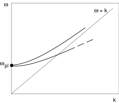
Figure 28: Plasmon spectrum.

The true pattern of plasmon collective modes is shown in Fig.28. A similar picture holds for plasminos.

Observability.

One-loop dispersive curves are gauge-invariant. However, the question whether these curves are physically observable is, again, highly non-trivial. It is easy to measure explicitly photon dispersive curves in usual plasma — to this end, one should study propagating classical electromagnetic waves, measure the electric charge density (say, by laser beams) as a function of time and spatial coordinates and determine thereby the frequency and the wave vector of the wave.

But there is no such thing in Nature as classical gluon field due to confinement, and no classical device which would measure the color charge density exists. Even more obviously, quark fields (which have Grassmanian nature) cannot be treated classically. Hence, one cannot really measure the energy and momentum of propagating colored waves in a direct physical experiment.

What one can measure are correlators of colorless (in the first place, electromagnetic) currents. Modification of dispersive laws affects these correlators and that can be observed. However, a colorless current always couples to a pair of colored particles and, as a result, physical correlators involve some integrals of quark and gluon Green’s functions which are related to quark and gluon dispersive characteristics only in an indirect way. Also, thermal modification of vertices is as important here as modification of the Green’s functions.

However, there is one special point on the dispersive curves which can in principle be directly measured in experiment. This is the point on the longitudinal plasmino curve where its frequency acquires a minimal value and the group velocity turns to zero. Consider the problem of emission of relatively soft $e^{+}e^{-}$ or $\mu^{+}\mu^{-}$ pairs by $QGP$. In a “thermos bottle” gedanken experiment, one should make sure that the size of your thermos bottle is much less than the lepton mean free path. Otherwise, the leptons are thermalized and their spectrum is just Planckian. Btt in heavy ion collisions experiments, $QGP$ is produced in small volume, the condition $L_{\rm char}\ll L^{em}_{\rm free\ path}$ is satisfied, and the spectrum of emitted leptons (and photons) can provide a non-trivial information on dynamic characteristics of $QGP$.

The spectrum of soft dileptons was calculated in [172]. This is one of very few physical problems we know of where the hard thermal loop resummation technique [171] should be used (and was used) at full length. The spectrum feels the effects due to quark and gluon interactions in the region $E_{l^{+}l^{-}}\sim P_{l^{+}l^{-}}\sim gT$ — the spectrum at larger energies and momenta is the same as for the gas of free quarks. One particular source of soft dileptons is the process $q^{*}_{\bot}\to q^{*}_{\|}\ +\ l^{+}l^{-}$. The probability of this process has a “spike” for the momentum of $q_{\bot}^{*}$ and $q_{\|}^{*}$ coinciding with the momentum $k^{*}$ on the longitudinal plasmino dispersive curve with zero group velocity. There are just many plasminos at the vicinity of this point and the phase space factor provides a singularity at $E_{l^{+}l^{-}}=\omega_{\bot}(k^{*})-\omega_{\|}(k^{*})$ in the spectrum. Another spike comes from the process when a longitudinal plasmino with momentum $k^{*}$ annihilates with a longitudinal antiplasmino with the opposite momentum to produce a lepton pair with zero net momentum and the energy $2\omega_{\|}(k^{*})$.

Unfortunately, in the soft region, the main contribution in the spectrum is due to cuts. In other words, the most relevant elementary kinetic processes are not $q^{*}\to q^{*}+l^{+}l^{-}$ or $q^{*}+\bar{q}^{*}\to l^{+}l^{-}$, but rather $q^{*}+g^{*}\to q^{*}+g^{*}+l^{+}l^{-}$ etc. The spikes actually have finite width due to collisional damping of collective excitations (the issue to be discussed in the next section), and one can hope to see only a tiny resonance on a huge background. Still, such a resonance in the spectrum is an observable effect.

6.4 Damping mayhem and transport paradise.

Direct decay.

In the previous section, we discussed the Landau damping contribution to the imaginary parts of polarization operators and, correspondingly, to imaginary parts of dispersion laws. It comes from the kinematic region $\omega<k$ and is physically related to absorption of ingoing excitations by thermal quanta like in (6.57). However, we did not say a word about the contribution of direct decay processes $g^{*}\to q+\bar{q}$ etc. in the timelike kinematic region $\omega>k$.

That was with a good reason. On the one-loop level, the contribution of decay processes in imaginary parts is nonzero and is of order $\sim g^{2}T$. Unfortunately, it depends on the gauge and, in some gauges, has even the wrong sign corresponding not to damping of excitations but to instabilities [173]. The point is that such one-loop calculation is unstable with respect to higher-order corrections. It is very clear physically — quarks and gluons in $QGP$ cannot be treated as massless but acquire dynamical masses due to thermal effects. And the decay of a plasmon or plasmino into two other collective excitations is not kinematically allowed. The only exception is the process $g^{*}\to q^{*}+\bar{q}^{*}$ which in principle may go if [170]

$$N_{f}>9c_{F}-2c_{V}=6$$ (6.58)

But there are at most three light flavors in real $QGP$ and decay processes can be safely forgotten.

Collisional damping.

Still, damping is there even in the timelike region $\omega>k$ due to collisions $g^{*}+q^{*}\to g^{*}+q^{*}$, $q^{*}+\bar{q}^{*}\to g^{*}+g^{*}$ etc. This is also the main source of damping of transverse electromagnetic waves in usual plasma [22]. A rough estimate for collisional damping in $QGP$ can be done very simply.

The meaning of damping is the inverse lifetime of excitations. We have

$$\zeta\sim(\tau_{life})^{-1}\sim n\sigma^{tot}$$ (6.59)

where $n\sim T^{3}$ is the density of the medium and $\sigma^{tot}$ for excitations which carry (color) charge has a Coulomb form

$$\sigma^{tot}\sim g^{4}\int\frac{dp_{\bot}^{2}}{p_{\bot}^{4}}\sim\frac{g^{2}}{T^{2}}$$ (6.60)

We took into account the fact that the power infrared divergence for the integral of Coulomb cross section is effectively cut off at $p_{\bot}\sim gT$ due to Debye screening . As a result, we obtain the estimate

$$\zeta^{q,g}\sim g^{2}T$$ (6.61)

Note that this value for the damping is unusually large. It is much larger than, say, the damping of photons in ultrarelativistic $e^{+}e^{-}$ – plasma. The latter can also be estimated from the formula (6.59), but $\sigma^{tot}$ is now not the Coulomb, but the Compton cross section. The integral has now the form $\int_{eT}dp_{\bot}^{2}/p_{\bot}^{2}\sim\ln(1/e)$ and the estimate is

$$\zeta^{\gamma}\sim e^{4}T\ln(1/e)\ll e^{2}T$$ (6.62)

The question arises whether the new anomalously large scale $\sim g^{2}T$ has a  physical  relevance . We will return to discussion of this point a bit later.

2

Figure 29:

An accurate calculation of the damping of fast moving ($k\gg gT$) quark and gluon excitations in $QGP$ has been done in [170, 174] (see also [175]). Consider the graph in Fig.29 for the quark polarization operator where the lines with blobs stand for quark and gluon propagator dressed by thermal loops. The imaginary part of the loop in Fig.29 depends on the imaginary parts of internal propagators. The imaginary part of the gluon propagator due to Landau damping turns out to be of paramount importance. Physically, this contribution just corresponds to the scattering processes $g^{*}+q^{*}\to g^{*}+q^{*}$ and $g^{*}+g^{*}\to g^{*}+g^{*}$ as can be easily inferred if spelling out the exact gluon propagator as in Fig.30 (there is also a similar graph with internal gluon loop).

2

Figure 30: A graph contributing to ${\rm Im}\ \Sigma(k)$. Crossed lines are put on mass shell. One of the quarks in the internal loop has a negative energy.

Dressing the quark propagator (indicated by the blob in Fig.30) is important. If not taking it into account, the imaginary part of the propagator is $\delta$ – function and the result for ${\rm Im}\ \Sigma_{R}(\omega,{\bf k})$ near the mass shell $\omega=|{\bf k}|$ has the form

$${\rm Im}\ \Sigma_{R}({\bf k})=-\frac{3}{32\pi^{2}}\omega_{pl}^{2}g^{2}c_{F}T\gamma^{0}\int_{-\infty}^{\infty}dp_{0}\int_{-1}^{1}d\cos\theta\int_{0}^{\infty}\frac{dp^{2}}{p^{4}+\frac{9}{16}\omega_{pl}^{4}\frac{p_{0}^{2}}{p^{2}}}\ \delta(p_{0}-p\cos\theta)$$ (6.63)

where $\theta$ is the angle between ${\bf k}$ and ${\bf p}$. The integral has a power infrared behavior at $p\gg gT$, but this divergence is cut off due to Landau damping effects (the second term in the denominator in the integrand). Still, the integral in (6.63) diverges logarithmically at $p\ll gT$ and the result for the damping inferred from Eq.(6.63) is infinite.

The crucial observation is that the dressed quark propagator does not have singularities on the real $p_{0}$ axis. A self-consistent account of the collisional damping for the quark Green’s function moves its singularities in the complex plane. As a result, $\delta$ – function in the integrand is replaced by a smooth distribution with the width of order $\zeta\sim g^{2}T$:

$$\delta(p_{0}-p\cos\theta)\ \to\ \frac{\zeta/\pi}{(p_{0}-p\cos\theta)^{2}+\zeta^{2}}$$ (6.64)

This smoothing cuts off the logarithmic singularity in (6.63) at $p\sim g^{2}T$. The other source for the cutoff could be provided by magnetic screening effects , but the latter is an essentially nonabelian phenomenon whereas the cutoff due to smearing out the $\delta$ – function is a universal effect which occurs also in an abelian theory.

Note that the cutoff $p\ ^{>}_{\sim}\ g^{2}T$ corresponds to the cutoff $p_{0}$ $\ {}^{>}_{\sim}\ g^{4}T$. Really, the integral in (6.63) is saturated by the values $p$ and $p_{0}$ such that two terms $p^{4}$ and $\sim\omega_{\rm pl}^{4}p_{0}^{2}/p^{2}$ in the denominator in the integrand are of the same order. That means that $p_{0}^{\rm char}\sim p^{3}/\omega_{\rm pl}^{2}$ which gives the estimate $p_{0}\sim g^{4}T$ at the lower range of integration. Actually, our calculation corresponds to picking up the pole corresponding to the so called attenuating mode

$$p_{0}=-i\frac{4}{3}\frac{p^{3}}{\omega_{\rm pl}^{2}}$$ (6.65)

of the exact gluon propagator in the graph in Fig.29. This pole presents an extra solution of the transverse dispersive equation in Eq.(6.3) when the imaginary part of the logarithm in $\Pi_{t}(p_{0},p)$ which is responsible for Landau damping is taken into account, and we assumed $|p_{0}|\ll p$. The attenuating mode (6.65) was found in [170]. It exists in the region $g^{2}T\ ^{<}_{\sim}\ p\ ^{<}_{\sim}\ gT$ and the dispersion law (6.65) holds in the region $g^{2}T\ \ll\ p\ \ll\ gT$. When $p\ ^{>}_{\sim}\ gT$, the assumption $|p_{0}|\ll p$ is not fulfilled, and when $p\ ^{<}_{\sim}\ g^{2}T$, perturbation theory breaks down. A similar mode exists also in nonrelativistic plasma (see Ref.[22], p.135). We will meet the mode (6.65) and the frequency scale $\sim g^{4}T$ once again in the end of this chapter when discussing chirality non-conservation rate.

To find the dispersion law, one should add $i{\rm Im}\ \Sigma_{R}({\bf k})$ from Eq.(6.63) to the one-loop result for $\Sigma_{R}(k)$ (which is real for $\omega\geq k$) and solve the dispersive equation ${\rm Det}\|\gamma^{0}\omega-\mbox{\boldmath$\gamma$}{\bf k}-\Sigma_{R}({\bf k})\|\ =\ 0$. The solution is complex $\omega^{pole}(k)=\omega^{1\ loop}(k)-i\zeta(k)$ and the final result for $\zeta(k\gg gT)$ is very simple.

$$\zeta^{q}=\alpha_{s}c_{F}T\ln(C^{q}/g)$$

$$\zeta^{g}=\alpha_{s}c_{V}T\ln(C^{g}/g)$$ (6.66)

(damping of gluon fast moving excitations can be calculated along the same lines). Only the coefficient of logarithm can be calculated. The constants $C^{q},\ C^{g}$ under the logarithm cannot be determined. Actually, we will see shortly that these constants are gauge–dependent and cannot be defined in a reasonable way.

2

Figure 31: Polarization operator of soft plasmino.

The results (6.4) were obtained solving the dispersive equation with the polarization operator (6.63) calculated at real $\omega$. A more refined analysis which takes into account the modification of ${\rm Im}\ \Sigma(k)$ for complex $\omega$ when one starts to move from the real $\omega$ axis towards a singularity shows that the dispersive equation has actually no solutions and the singularity is no longer a pole, but a branching point [176, 177, 178]. But this branching point is located at the same distance from the real axis as the would-be pole and brings about the same damping behavior of the gluon retarded Green’s function $G^{R}(t)\sim\exp\{-\zeta t\}$ at large real times.

The modification of the fermion propagator due to higher loops in the graphs in Fig.29, 30 was taken into account smearing out the $\delta$ – function singularity in the Green’s function as in Eq.(6.64). In recent [179] it was found that if doing things quite carefully, namely resumming leading infrared divergent pieces in the soft photon loops contributing in the fermion Green’s function in any order in abelian theory, the infrared divergence in (6.63) eventually survives. That essentially means that $G^{R}(\omega)$ does not involve singularities at all at finite distance from the real axis. This results in a non-exponential decay of $G^{R}(t)$ at large real time:

$$G^{R}(t)\sim\exp\{-\alpha Tt\ \ln(eTt)\}$$ (6.67)

In spite of the fact that this result is rather unexpected, it seems to be correct. Non-standard logarithmic factor in (6.67) resembles the logarithmic factor in the exponent in (6.23) . An analogy can also be drawn with the well-known logarithmic divergence in the phases of Coulomb scattering [180]. A careful independent study of this question is, however, highly desirable.

Damping of excitations in another kinematic region ${\bf k}=0$ (“standing” plasmons and plasminos) was studied in [171]. Here the vertex corrections are as important as corrections to the propagators, however an accurate analysis of [171] shows that it suffices to take into account only one (hard thermal) loop corrections both in polarization operators and vertices. Consider for definiteness the damping of standing plasminos. The graphs contributing to the soft plasmino polarization operator are shown in Fig.31. Using Keldysh technique one can derive in the limit of soft external momentum

$$\Sigma^{R}(k)=-2ig^{2}\int\frac{d^{4}q}{(2\pi)^{4}}\frac{T}{q}_{0}{\rm Im}\ D_{\mu\nu}^{R}(q)\left[\frac{1}{2}\Gamma^{R}_{\mu\nu}(k;q)+\right.$$

$$\left.\Gamma^{R}_{\mu}(k,k+q;q)G^{R}(k+q)\Gamma_{\nu}^{R}(k+q,k;-q)\right]$$ (6.68)

Here $\Gamma^{R}$ are the retarded vertices presenting certain combinations of the Keldysh components $\Gamma_{\mu}^{abc}$ and $\Gamma_{\mu\nu}^{abcd}$:

$$\Gamma_{\mu}^{R}\ =\ \sum_{b,c=1}^{2}\Gamma_{\mu}^{1bc},\ \ \ \ \ \ \Gamma_{\mu\nu}^{R}\ =\ \sum_{b,c,d=1}^{2}\Gamma_{\mu\nu}^{1bcd}$$ (6.69)

where the index 1 is put on the outgoing fermion line. Like retarded propagators, $\Gamma^{R}$ are analytic in the upper $\omega$ half–plane. Substituting here transverse and longitudinal parts of the gluon Green’s function and one-loop vertices $\Gamma_{\mu\nu}$ and $\Gamma_{\mu}$, calculating the integral (which in this case can be done only numerically), and solving the dispersive equation, one arrives at the result

$$\zeta^{q}(k=0)=1.43c_{F}\frac{g^{2}T}{4\pi}$$ (6.70)

However, the gluon Green’s function involves also a gauge-dependent part

$$D_{\mu\nu}^{R(\alpha)}(q)=(\alpha-1)\frac{q_{\mu}q_{\nu}}{[(q_{0}+i\epsilon)^{2}-{\bf q}^{2}]^{2}}$$ (6.71)

where $\alpha$ is a gauge parameter and an infinitesimal $i\epsilon$ is introduced to provide for the right analytical properties. At first sight, this gauge-dependent piece should not affect the position of the pole. Really, one can use the Ward identities

$$q_{\mu}\Gamma_{\mu}^{R}(k,k+q;q)\ =\ t^{a}\left\{[G^{R}(k+q)]^{-1}-[G^{R}(k)]^{-1}\right\}$$

$$q_{\mu}\Gamma_{\mu\nu}^{R}(k;q)\ =\ t^{a}\left\{\Gamma_{\nu}^{R}(k,k-q;-q)-\Gamma_{\nu}^{R}(k+q,k;-q)\right\}$$ (6.72)

which hold also at finite temperature for retarded propagators and vertices [181, 174] to derive

$$\Sigma^{R(\alpha)}(k)=-ig^{2}Tc_{F}(\alpha-1)[G^{R}(k)]^{-1}\times$$

$$\int\frac{d^{4}q}{(2\pi)^{4}}\frac{1}{q}_{0}\left\{\frac{1}{[(q_{0}+i\epsilon)^{2}-{\bf q}^{2}]^{2}}-\frac{1}{[(q_{0}-i\epsilon)^{2}-{\bf q}^{2}]^{2}}\right\}\left[G^{R}(k+q)-G^{R}(k)\right][G^{R}(k)]^{-1}$$ (6.73)

We see the presence of factors $[G^{R}(k)]^{-1}$ both on the right and on the left. $G^{R}(k)$ is singular at the pole and $[G^{R}(k)]^{-1}$ is zero. One might infer from this that a gauge-dependent contribution to $\Sigma^{R}({\rm pole})$ and hence to the corresponding solution of the dispersive equation determining the pole position is also zero.

However, this is wrong [182, 177]. The point is that the integral in (6.4) involves a severe power infrared divergence and is infinite at the pole. We have thereby a $0\times\infty$ uncertainty. This uncertainty can be resolved by choosing $k$ not exactly at the pole but slightly off mass shell. Then $[G^{R}(k)]^{-1}$ is not exactly zero and also the divergence in the integral is cut off by an off-mass-shellness. When the distance from the mass shell is small, the final result for $\Sigma^{R(\alpha)}(k\to{\rm pole})$ does not depend on this distance and is just finite. In the soft momenta region

$$\Sigma^{R(\alpha)}_{\rm soft}(k)=-\frac{i(\alpha-1)g^{2}Tc_{F}}{4\pi}\gamma^{0}$$ (6.74)

This brings about a gauge-dependent part $\sim g^{2}T$ in the damping of soft plasminos. A similar analysis with the same conclusion can be carried out for plasmons.

In Ref.[183], another regularization procedure was suggested where the external momentum $k$ was always kept strictly on mass shell, but the divergent integral in Eq.(6.4) was regularized introducing an explicit infrared cutoff $\mu$. Then, of course, a gauge–dependent piece is absent even after the cutoff is eventually sent to zero. It does not solve a problem, however. The physical definition of damping (if any) should be related to the exponential asymptotics of $G^{R}(t)$ at large real times. $G^{R}(t)$ is given by the Fourier integral over the real $\omega$ axis

$$G^{R}(t)\ =\ \int_{-\infty}^{\infty}G_{R}(\omega)\ e^{-i\omega t}\ d\omega$$

Thus it is determined by the behavior of $G_{R}(\omega)$ at real $\omega$, i.e. off mass shell. The damping defined as

$$\zeta\ =\ -\lim_{t\to\infty}\ \frac{G_{R}(t)}{t}$$

is gauge–dependent [177].

The same gauge-dependence shows up in the damping of energetic plasmons and plasminos, but in the latter case, this gauge-dependence is parametrically overwhelmed by the leading gauge-independent contribution (6.4) involving the factor $\ln(1/g)$.

Observability.

The observed gauge-dependence of the damping obviously indicates that it is not a physical quantity. This is definitely true at least for soft plasmons and plasminos where the gauge-dependent part and the gauge-independent part (6.70) are of the same order $\sim g^{2}T$.

Indeed, it is not possible to contemplate a physical experiment where this quantity could be measured. That should be confronted with the case of abelian plasma where damping of electromagnetic waves is a perfectly physical quantity and can be directly observed by measuring the attenuation of the amplitude of a classical wave with time. But as we already noted, no classical gluon or quark waves exist. This observation refers also for the damping of electron and positron collective excitations in the ultrarelativistic abelian plasma. It also has an anomalously large scale $\sim e^{2}T$ [with the extra logarithmic factor  $\ln(1/e)$ for $k\gg eT$] and it also cannot be directly measured.

One could try to observe the effects due to damping in gauge-invariant quantities like the polarization operator of electromagnetic currents. An accurate analysis which goes beyond the conventional hard thermal loop resummation technique and effectively resums a set of ladder graphs shows, however, that a self-consistent account of the corrections due to damping in the quark Green’s functions and in the vertices results in the exact cancelation of the anomalously large scale $\sim g^{2}T$ in the final answer [174]. (for a similar analysis with a similar conclusion in scalar QED see [184]).

However, there is a physical problem where the scale $\sim g^{2}T$ can in principle show up. This is the already discussed problem of lepton pair production in $QGP$. We have seen that the spectrum of leptons pairs involves spikes associated with a special point with zero group velocity on the longitudinal plasmino dispersive curve. Going beyond the hard thermal loop approximation and taking into account the effects due to collisional damping in the Green’s functions and in the vertices would bring about a finite width for these spikes of order $g^{2}T$ and there is a principle possibility to measure this width. This problem has not been studied, and it is not clear by now whether the width of the spike can be calculated analytically and whether one can single out this spike out of the background.

What one can say quite definitely is that this width should crucially depend both on modification of propagators due to collisional effects and on a similar modification of vertices and has little to do with the (gauge-dependent) position of the pole (or whatever the real singularity is [176, 177, 178]) of the quark and gluon Green’s function.

Thus we are convinced that the latter is not a physical quantity probably even for energetic plasmons in spite of the fact that the leading contribution (6.4) is gauge-independent there. We just do not know how on earth this quantity could be measured.

Transport phenomena.

There is a lot of kinetic phenomena in $QGP$ which are physical and measurable. Indeed, nothing in principle prevents measuring the electric resistance of a vessel with $QGP$ or studying the flow of $QGP$ through narrow tubes. They do not depend, however, on the anomalous damping scale $g^{2}T$, but rather on a much smaller scale

$$(\tau_{char})^{-1}\sim g^{4}T\ln(1/g)$$ (6.75)

This scale already appeared in (6.62) determining the damping of electromagnetic waves in $e^{+}e^{-}$ – plasma. And it is also the scale which determines the mentioned physical effects of viscosity and electric conductivity, and many others — heat conductivity, energy losses of a heavy particle moving through plasma, etc.

The appearance of the scale $g^{4}T\ln(1/g)$ has a clear physical origin. All the mentioned effects are inherently related to the rate of relaxation of the system to thermal equilibrium. The latter can be estimated as

$$(\tau_{rel})^{-1}\sim n\sigma^{trans}$$ (6.76)

It looks the same as the estimate for lifetime (6.59) but with an essential difference — in contrast to (6.59), the estimate (6.76) involves the transport rather than the total cross section. The transport cross section is defined as

$$\sigma^{trans}=\int d\sigma(1-\cos\theta)$$ (6.77)

where $\theta$ is the scattering angle. The factor $(1-\cos\theta)$ takes care of the fact that small–angle scattering though contributes to the total cross section, does not essentially affect the distribution functions $n_{g}({\bf p})$, $n_{q}({\bf p})$ and is not effective in relaxation processes. For the Coulomb scattering in ultrarelativistic plasma, the transport cross section is

$$\sigma^{trans}\sim g^{4}\int_{(gT)^{2}}\frac{dp_{\bot}^{2}}{p_{\bot}^{4}}\frac{p_{\bot}^{2}}{T^{2}}\sim\frac{g^{4}}{T^{2}}\ln\frac{1}{g}$$ (6.78)

Multiplying it by $n\sim T^{3}$ and substituting it in (6.76), the estimate (6.75) is reproduced.

Viscosity and all other similar quantities can be calculated analytically in the leading order (probably, magnetic infrared divergences prevent an analytic evaluation of these quantities in next orders in $g$, but this question is not yet well studied). It is interesting that Feynman diagram technique proves to be technically inconvenient here , and the good old Boltzmann kinetic equation is the tool people usually use (see e.g. [185]).

Let us make two illustrative estimates which make clear how the relaxation scale (6.75) depending on the transport cross section (6.78) arises.

First, let us estimate the electric conductivity of $QGP$ (it is the quite conventional conductivity, not the “color conductivity” which is sometimes discussed in the literature, depends on the anomalous damping scale $g^{2}T$, and is not a physically observable quantity — we do not have batteries with color charge at our disposal). Suppose at $t=0$ the system was at thermal equilibrium so that the quark distribution functions are $n_{0}({\bf p},{\bf x},t=0)=n_{F}(|{\bf p}|)$. When we switch on the electric field, the distribution function starts to evolve according to the kinetic equation

$$\frac{\partial n({\bf p},{\bf x},t)}{\partial t}+{\bf v}\frac{\partial n({\bf p},{\bf x},t)}{\partial{\bf x}}=e{\bf E}\frac{\partial n({\bf p},{\bf x},t)}{\partial{\bf p}}+\ldots$$ (6.79)

with ${\bf v}={\bf p}/|{\bf p}|$. Dots in RHS of Eq.(6.79) stand for the collision term which becomes relevant at $t\sim x\sim\tau_{\rm rel}\sim\tau_{\rm free\ path}\sim[g^{4}T\ln(1/g)]^{-1}$. Thus the electric field brings about distortions of the distribution function which grow up to the characteristic value

$$\delta n\sim e{\bf E}\frac{{\bf v}}{T}n_{0}\tau_{\rm free\ path}\sim\frac{eT{\bf E}{\bf v}}{g^{4}\ln(1/g)}$$

At this point, collisional effects stop the growth (a particle drifting in external electric field collides with a particle in the medium, forgets what happened before, and starts drifting anew). The density of electric current in the medium is

$${\bf j}=e\int{\bf v}\delta n\ d^{3}p\sim{\bf E}\frac{e^{2}T}{g^{4}\ln(1/g)}$$ (6.80)

The coefficient between ${\bf j}$ and ${\bf E}$ gives the conductivity.

Let us estimate now the energy losses of a heavy energetic quark in $QGP$. Of course, free quarks do not exist, but a physical experimental setup would be sending into the bottle with $QGP$ a heavy meson ${Q}\bar{q}$ with open beauty or top. In $QGP$, the meson dissociates, and a naked heavy quark propagates losing its energy due to interaction with the medium. It goes out then on the other side of the bottle dressed again with light quarks, but not necessarily in the same way as before. When $M_{Q}\gg\Lambda_{QCD}$, this dressing does not essentially affect its energy. A heavy particle containing $Q$ can be detected and its energy can be measured.

Suppose a heavy quark is ultrarelativistic, but its energy is not high enough for the Cerenkov radiation processes to be important. Then the energy would be lost mainly due to individual incoherent scatterings. The mean energy loss in each scattering is $\Delta E\sim T$ ($T$ — is a characteristic energy of the particles in heat bath on which our heavy quark scatters). The mean time interval between scatterings is $\tau_{\rm free\ path}\sim[g^{4}T\ln(1/g)]^{-1}$. We obtain

$$-\frac{dE}{dx}\sim\frac{\Delta E}{\tau_{\rm free\ path}}=C\alpha_{s}^{2}T^{2}\ln(1/g)$$ (6.81)

This estimate turns out to be correct up to the argument of the logarithm which in reality is energy–dependent [186]. The numerical coefficient $C=4\pi c_{F}/3$ was determined by Bjorken [187]

6.5 Chirality drift.

Up to now, we were concentrated mainly on the perturbative calculations in $QGP$. Also we discussed the magnetic screening phenomenon which, as was explained in Sect. 6.1, is essentially non- perturbative. Magnetic screening scale $\sim g^{2}T$ shows up in static correlators of different quantities at large distances. Magnetic screening also affects kinetic characteristics of $QGP$ such as plasmon and plasmino dispersion laws, transport coefficients etc. The latter are well– defined and analytically calculable in the lowest perturbative order. The problems appear (and non–perturbative physics come into play) only when trying to determine higher–order corrections. There is, however, a beautiful kinetic effect which is purely non–perturbative. This is the axial charge non– conservation in hot quark–gluon plasma, or the “chirality drift” presenting the subject of this conclusive section.

Theoretical picture.

The primary practical interest of this quantity is related not to $QCD$, but to the dynamics of electroweak theory in early hot Universe. Long time ago, ‘t Hooft observed [145] that the baryon charge is conserved in standard model only on the classical lagrangian level. It is not conserved in the full quantum theory due to anomaly

$$\partial_{\mu}j_{\mu}^{B}\ =\ \frac{g^{2}}{32\pi^{2}}G_{\mu\nu}^{a}\tilde{G}_{\mu\nu}^{a}$$ (6.82)

where $G_{\mu\nu}^{a}$ is the $SU(2)$ electroweak field. Baryon number non-conservation is precipitated by the gauge field configurations with nonzero Pontryagin number, the instantons. At zero temperature, the action of electroweak instantons is very large $\sim 2\pi/\alpha_{W}$ and the rate of baryon number non-conservation involves the exponential factor $\sim\exp\{-2\pi/\alpha_{W}\}$ which is zero in all practical sense.

Physically, instantons present tunneling trajectories through a barrier in the functional space. This barrier is associated with a collective degree of freedom called Chern–Simons number

$$Q\ =\ \frac{g^{2}}{32\pi^{2}}\epsilon_{ijk}\int d^{3}x\left[G_{ij}^{a}A_{k}^{a}\ -\ \frac{g}{3}\epsilon^{abc}A_{i}^{a}A_{j}^{b}A_{k}^{c}\right]$$ (6.83)

The integrand in (6.83) is not gauge invariant, but $Q(t)$ itself is invariant under topologically trivial gauge transformations. The classical energy functional in Yang–Mills theory has degenerate minima at integer $Q$ (see Fig.32). These minima are related to each other by topologically non-trivial gauge transformations. In electroweak theory where gauge symmetry is broken spontaneously by the Higgs mechanism , high barrier between adjacent minima is created. The top of the barrier between, say, the minima with $Q=0$ and $Q=1$ (actually, it is a saddle point in the functional space with only one unstable mode) is called the sphaleron [188] and has the energy $E_{\rm sph}\ \sim\ m_{W}/\alpha_{W}$. Chern–Simons number of the sphaleron configuration is $Q_{\rm sph}=1/2$.

Figure 32: A schematic representation of the (bosonic) potential energy along a particular direction (labeled $z$) in field space, corresponding to topologically non-trivial transitions between vacua.

It was observed in [189] that, when the temperature grows, the height of the barrier decreases. Baryon number non-conservation processes are thus greatly facilitated. Actually, as soon as $T\gg m_{W}$, the leading contribution in the rate comes not from quantum tunneling processes “through” the barrier, but from the classical thermal jumps “over” the barrier. These classical transitions are stochastic in nature and can occur both with increasing and decreasing of baryon number. We have the physical picture of Brownian motion. Baryon charge “drifts” so that the average square of the fluctuation of the baryon charge $[B(t)-B(0)]^{2}$ grows linearly with time. Due to the algebraic identity

$$\dot{Q}\ =\ \frac{g^{2}}{32\pi^{2}}\int d^{3}xG_{\mu\nu}^{a}\tilde{G}_{\mu\nu}^{a}\ =\ \dot{B},$$ (6.84)

one can study alternatively the fluctuations of Chern– Simons number $Q(t)$. The rate of baryon number non-conservation $\Gamma^{\Delta B\neq 0}(T)$ is defined as the coefficient of the large time asymptotics of the thermal correlator

$$C(t)\ =\ <[Q(t)-Q(0)]^{2}>_{T}\ \stackrel{{\scriptstyle{\rm large}\ t}}{{\longrightarrow}}\ \Gamma^{\Delta B\neq 0}(T)Vt,$$ (6.85)

where $V$ is the spatial volume of the system (naturally, the larger is the volume, the larger is the net rate), and we subtracted the time–independent part. In the temperature region $m_{W}(T)\ll T\ll E_{\rm sph}(T)$, the estimate for the rate is $\Gamma^{\Delta B\neq 0}(T)\propto\exp\{-E_{\rm sph}(T)/T\}$. At some temperature (which is close to the critical temperature $T_{c}$ where the spontaneously broken gauge symmetry $SU(2)\otimes U(1)$ is restored), the characteristic energy of the excitations is of the same order as the barrier height at which point the exponential suppression disappears. An accurate calculation of the rate in the temperature region where the suppression is still there was performed in [190].

The question arises what happens at large temperatures $T\gg T_{c}$ where no barrier exists and the quasi-classical approximation breaks down. It was argued in [190] that the rate behaves as

$$\Gamma^{\Delta B\neq 0}(T)\ =\ \kappa(\alpha_{W}T)^{4}$$ (6.86)

where $\kappa$ is a constant which cannot be calculated analytically. The rate (6.86) is a purely non-perturbative quantity. One can show that the rate $\Gamma^{\Delta B\neq 0}(T)$ defined in (6.85) is zero in any order of perturbation theory. The rate (6.86) is large, it leads to the dissipation of any primordial baryon charge density (if $B-L$ is exactly conserved as it does in most models of grand unification under discussion) and makes our very existence problematic. I will not pursue the discussion of this issue further here and refer the reader to a comprehensive review [193].

The estimate (6.86) can be obtained as follows. As was mentioned, the barrier does not exist at high $T$. There are field configurations ${\bf A}({\bf x})$ with arbitrary small energy which have $Q=1/2$ and interpolate between adjacent minima. Such configurations should have, however, large spatial size: the larger is the size, the smaller are characteristic field gradients and the smaller is the energy $E\sim\int d{\bf x}(\partial A)^{2}$. One can visualize these configurations as the slices $\tau=0$ of the standard BPST instantons in the hamiltonian gauge $A_{0}=0$. It is easy to see that the energy of such a slice for the instanton of size $\rho$ is $E(\rho)\sim 1/(\alpha_{W}\rho)$. Writing the integral over the collective coordinate $\rho$ with the standard zero temperature instanton measure $\sim\int d\rho/\rho^{5}$ (see Ref.[195]), we obtain

$$\Gamma^{\Delta B\neq 0}(T)\ \sim\ \int\frac{d\rho}{\rho^{5}}\exp\left\{-\frac{1}{\alpha_{W}\rho T}\right\}\ \sim\ (\alpha_{W}T)^{4}$$ (6.87)

The characteristic $\rho$ where the integral is saturated is nothing else as our old friend, the magnetic screening scale. Actually, one can forget at this point, if one wishes, about electroweak theory altogether. In the high temperature region, it presents “electroweak plasma”, and its physics is basically the same as the physics of $QGP$ which is of main interest for us here. Instead of baryon number non-conservation, we have here the axial charge non-conservation. Like baryon charge, it is conserved on the classical lagrangian level in the theory with massless quarks and is not conserved in the full quantum theory due to $U_{A}(1)$ anomaly. The rate of axial charge non-conservation in hot $QCD$ can be determined from the asymptotics of the Chern–Simons correlator (6.85) at large Minkowski times.

The result (6.86) means that roughly one transition occurs in the volume $\sim(g^{2}T)^{-3}$ by the time $\sim(g^{2}T)^{-1}$. The estimate for the characteristic volume seems to be rather solid: indeed, the barrier becomes irrelevant and also perturbation theory breaks down at the scale $\rho\sim(g^{2}T)^{-1}$. However, the estimate for the characteristic time of the transition $t_{\rm char}\sim(g^{2}T)^{-1}$ was recently criticized in [196]. The time $t\sim(g^{2}T)^{-1}$ is the characteristic time of smearing out the wave packet with the size $\rho\sim(g^{2}T)^{-1}$ in empty space. But our space is not empty, it presents a heat bath densely packed with gluon and quark excitations. It was argued in Ref.[196] that the time it takes for a quasi-sphaleron to decay in quark-gluon plasma plasma is actually suppressed by two powers of $g$ and is estimated as

$$t_{\rm decay}\ \sim\ (g^{4}T)^{-1}$$ (6.88)

Correspondingly, the new estimate for the rate is

$$\Gamma\ \sim\ \frac{1}{\rho_{\rm char}^{3}}\frac{1}{t_{\rm decay}}\ \sim\ \alpha^{5}T^{4}$$ (6.89)

The estimate (6.88) and its corrolary (6.89) can be obtained as follows. Suppose, we have at $t=0$ a wave packet with the size $\sim(g^{2}T)^{-1}$. Expand it in Fourier series and solve a classical equation of motion (which takes into account the heat bath effects) for an individual mode ${\bf A}_{k}$ with initial condition

$$\dot{{\bf A}}_{k}=0$$ (6.90)

The solution presents a sum of three exponentials

$${\bf A}_{k}(t)\ =\ \alpha_{1}\exp\{-C_{1}g^{2}Tt-i\omega_{\bot}(k)t)\}\ +\ \alpha_{2}\exp\{-C_{2}g^{2}Tt-i\omega_{\|}(k)t)\}$$

$$+\beta\exp\{-C_{3}g^{4}Tt\}$$ (6.91)

The first two terms correspond to standard transverse and longitudinal plasmons and involve a plasmon decay rate factor with $\zeta\sim g^{2}T$ while the third one corresponds to attenuating mode (6.65) with the decay rate $\sim g^{4}T$ at $k\sim g^{2}T$. The first and the second exponential come with small coefficient $\sim g^{2}$ due to the boundary conditions (6.90) and will die away at the time scale $\sim(g^{2}T)^{-1}$ while the second exponential is still alive. It would eventually determine the quasi-sphaleron decay rate.

In our own opinion, these arguments are not conclusive enough. Let us first modify the initial conditions and put $\dot{{\bf A}}_{k}\sim g^{2}T{\bf A}_{k}$. Such initial conditions seem to be as reasonable as (6.90). But then the coefficients $\alpha_{1,2}$ and $\beta$ would be of the same order and the Chern–Simons number of the field configuration (6.5) would be essentially modified on the time scale $(g^{2}T)^{-1}$ rather than $(g^{4}T)^{-1}$. Second, the amplitude of Fourier harmonics in quasi–sphaleron wave packet is large and their nonlinear interaction is essential. Even if we started up with only attenuating mode at the initial moment, normal plasmon modes would be excited due to nonlinear effects and would eventually determine the time decay scale.

Another question which can be asked here is why we assumed that the plasmon harmonics die away with the anomalous damping scale $\sim g^{2}T$ rather than with the scale $\sim g^{4}T$ which is characteristic for transport phenomena in plasma and which, as we repeatedly argued in the previous sections, is more physical. The point is that the latter scale depends on the transport cross section (6.77) where the region of small momentum transfer $p_{\bot}\sim gT$ is suppressed. In this particular problem, we do not see a reason to include such a suppression, however. The scale $gT$ is large compared to the characteristic momentum scale $g^{2}T$ determining chirality drift. When a mode acquires the momentum $\sim gT$, it is lost as far as the coherent quasi–sphaleron wave packet is concerned.

But all these arguments are extremely heuristic. To solve the problem accurately, it does not suffice to play around with small fluctuations on the vacuum background. Actually, one has to expand the field near the quasi–sphaleron background ${\bf A}\ =\ {\bf A}_{b}+\delta{\bf A}$ and to solve the linearized equations for $\delta{\bf A}$ in the heat bath.

Let us first see what happens in the absence of heat bath. Vast majority of the modes are stable. There are two directions in the functional space decreasing the energy of the field configuration. One of them corresponds to rescaling the quasi-sphaleron configuration and can be handled introducing the collective coordinate $\rho$ and integrating over it as in (6.87). The mode of main interest for us is the intrinsic sphaleron unstable mode $\delta{\bf A}_{unst}$ which corresponds to rolling down the slope away from the quasi-sphaleron ridge. In vacuum, the corresponding linearized equation is $\delta\ddot{{\bf A}}\ \sim\ [k_{\rm char}^{2}]\delta{{\bf A}}$ with $k_{\rm char}\sim g^{2}T$. It describes the decay of quasi–sphaleron by the time $\sim(g^{2}T)^{-1}$.

Let us now switch on the medium effects. The problem has not been accurately solved yet, but, taking insight from the dispersive equation (6.3) on the vacuum background, we can tentatively add to $k_{\rm char}^{2}$ the transverse polarization operator $\Pi_{t}(\omega,k_{\rm char})$. The new dispersive equation looks something like

$$-\omega^{2}\ =\ k_{\rm char}^{2}+\Pi_{t}(\omega,k_{\rm char})$$ (6.92)

It differs from Eq.(6.3) only by the sign of $\omega^{2}$ term. Substitute now here $\Pi_{t}(\omega,k_{\rm char})\sim-i\omega_{\rm pl}^{2}\omega/{k_{\rm char}}$ which is true at small $\omega\ll k_{\rm char}$. The solution to the dispersive equation (6.92) is

$$\omega\ \sim\ -\frac{ik_{\rm char}^{3}}{\omega_{\rm pl}^{2}}\ \sim\ -ig^{4}T$$ (6.93)

This mode corresponds to damping of the fluctuations $\delta{\bf A}$ with time so that a perturbed field tends asymptotically back to the quasi–sphaleron configuration ${\bf A}_{b}$. This mode has nothing to do with instability.

The dispersive equation (6.92) has also an unstable solution, but it corresponds to large $\omega\gg k_{\rm char}$ where $\Pi_{t}(\omega,k_{\rm char})\ \sim\ \omega_{\rm pl}^{2}$. The corresponding unstable mode is

$$\omega_{\rm unst}\ \sim\ i\omega_{\rm pl}\ \sim\ igT$$ (6.94)

Thus medium increases the rate of the quasi-sphaleron decay rather than decreases it. The estimate is

$$\Gamma\ \sim\ g^{7}T^{4}$$ (6.95)

This reasoning is quite parallel to the reasoning of Ref.[196], only the sign of $\Pi_{t}(\omega,k_{\rm char})$ in the dispersive equation (6.92) is chosen positive rather than negative. Negative sign would transform the damping mode (6.93) into an unstable one, and the estimate (6.89) would be reproduced.

By no means we want to insist here that it is the estimate (6.95) rather than (6.89) which is correct. Choosing the positive sign for $\Pi_{t}(\omega,k)$ in (6.92) looks more natural, but the thermal polarization operator corresponding to fluctuations on a quasi–sphaleron background (with the Green’s functions on a quasi–sphaleron background in the loops) could essentially differ from the vacuum one, and only its accurate calculation would solve the problem. It is possible that the the rate is suppressed compared to the estimate (6.86), and it is also possible that it is enhanced. The third possibility (which is actually the most attractive) is that plasma effects neither increase nor decrease the rate of decay, but leave it basically intact.

Numerical experiment. Kinetic equations.

Let us discuss now experimental (lattice) data. A very serious difficulty here is that the rate of baryon number (chiral charge) non- conservation is a kinetic quantity defined in real time. We are not able currently to calculate numerically field theory path integrals in Minkowski space- -time and have to look for some other way to solve the problem.

As was mentioned earlier, the physical mechanism of chirality non–conservation is the classical drift over the barrier. The idea arises to obtain the result just solving the classical equations of motion and looking at how the classical Chern–Simons charge (6.83) is changed with time. Performing an average over initial conditions with the classical weight $\sim\exp\{-\beta H^{\rm cl}\}$, one estimates the rate of the drift in hot field theory. This algorithm was suggested in [197] and successfully tested in some 2–dimensional models [197, 198]. In [191] and in recent [192], the same algorithm was applied to 4–dimensional gauge theories. To discretize the classical equations of motion, the system was put on a 3–dimensional hamiltonian lattice, the lattice spacing $a$ playing the role of the ultraviolet cutoff.

The question whether such a classical algorithm is justified or not is under discussion now. The main problem here are severe power ultraviolet divergences inherent for a classical field theory at finite $T$. A classical Rayleigh–Jeans ultraviolet divergence in the energy density of the photon gas

$$E^{cl}\ \sim\ \int d^{3}p|{\bf p}|\ n^{cl}_{B}(|{\bf p}|)\ \sim\ T\int d^{3}p\ \sim\ T\Lambda_{UV}^{3}$$ (6.96)

[where the classical limit of the Bose distribution is $n_{B}^{cl}(\epsilon)=1/(\beta\epsilon)$] was the reason to develop the quantum theory in the first place. Classical contribution to the plasma frequency

$$(\omega_{\rm pl}^{\rm cl})^{2}\ \sim\ g^{2}\int\frac{d^{3}p}{|{\bf p}|}\frac{1}{\beta|{\bf p}|}\ \sim\ g^{2}T\Lambda_{UV}$$ (6.97)

is also ultraviolet divergent.

In the full theory, the divergence is cut off at $|{\bf p}|\sim T$ (where quantum corrections in the Bose distribution function come into play). For the classical approximation to be justified, one should always keep $a^{-1}\sim\Lambda_{UV}\ll T$.

In principle, chirality non-conservation rate calculated by the classical algorithm could also be cutoff–dependent. Moreover, if the estimate (6.89) of Ref.[196] or the estimate (6.95) is correct, one should expect cutoff–dependence of $\Gamma$. In both cases, $\Gamma$ depends explicitly on the plasma frequency scale which is cutoff–dependent when calculated classically. One easily estimates

$$\Gamma_{\rm ASY}\ \sim\ g^{10}T^{4}\Longrightarrow\Gamma_{\rm ASY}^{\rm cl}\ \sim\frac{k_{\rm char}^{6}}{(\omega_{\rm pl}^{\rm cl})^{2}}\ \sim\ \frac{g^{10}T^{5}}{\Lambda_{UV}}$$

$$\Gamma_{(\ref{g7T4})}\ \sim\ g^{7}T^{4}\Longrightarrow\Gamma_{(\ref{g7T4})}^{\rm cl}\ \sim{k_{\rm char}^{3}}{\omega_{\rm pl}^{\rm cl}}\ \sim\ g^{7}T^{7/2}\Lambda_{UV}^{1/2}$$ (6.98)

However, if the original estimate (6.86) is not affected by the medium effects, $\Gamma$ does not depend on the plasma frequency scale, but only on the magnetic mass scale $g^{2}T$. In this case, one could expect that classical numerical results for $\Gamma$ do not depend on cutoff, and the whole algorithm is trustworthy if the condition

$$g^{2}T\ \ll\ \Lambda_{UV}\ \ll T$$

is satisfied.

Following the suggestion of [199], the question of whether classical rate depends on cutoff or not, was studied in [192]. Ambjorn and Krasnitz find that the rate depends neither on cutoff nor on $\omega_{\rm pl}$. Their answer for the rate is

$$\Gamma^{\Delta B\neq 0}(T)\ \approx\ 1.1(\alpha_{W}T)^{4}$$ (6.99)

This result directly contradicts the estimate (6.89) and also (6.95). It was suggested in [196] that the result (6.99) is actually a lattice artifact related to an imperfect lattice definition of the Chern–Simons number. It may be, though it is not quite clear why an alleged lattice artifact (6.99) does not depend on the lattice spacing.

On pure esthetic grounds, it would be much nicer if the plasma effects would not eventually influence the quasi-sphaleron decay rate and the original result (6.86) and the numerical calculations of [192] were correct. Our heuristic arguments which take into account not only the attenuating but also the plasmon modes and nonlinear interaction between them [see the discussion after Eq.(6.5)] also seem to indicate that. We would rather lay our bets on this possibility, but a scientific answer to this question is not yet found. Thus we are in a position to discuss what happens if an unfortunate possibility that the rate depends on the scale $\omega_{\rm pl}$ and thereby on the ultraviolet cutoff, when calculated classically, is realized. Can one still hope to suggest a numerical procedure where the rate of the chirality drift in the full quantum theory could be evaluated quantitatively ?

This question was studied in [199] (see also recent [200]). An algorithm based on the separation of low momentum and high momentum scale was suggested. The idea was to take into account explicitly the contribution of high momentum modes in the effective hamiltonian and then to solve numerically the classical equations of motion of this effective hamiltonian for soft modes.

The effective theory for soft modes (with momenta of order $gT$) was first formulated in [171, 181] in lagrangian form. This lagrangian involves multiple quark and gluon effective vertices of the kind shown in Fig.33. Characteristic momenta flowing in the hard thermal loop in Fig.33 are of order $T$. We already discussed at length two–point quark and gluon Green’s functions which are contained in this lagrangian [see Eqs.(6.3), (6.49)]. Both 2–point and also 3–point, 4–point etc. effective vertices are nonlocal.

Figure 33: An example of HTL graph contributing to the effective 3–gluon vertex. The loop momentum is hard $p\sim T$. External momenta are soft.

A nonlocal lagrangian is very inconvenient for a numerical study. Fortunately, it can be presented in a local form [201, 165]. The price is introducing new variables depending on $x$ and on an extra 3–dimensional unit vector ${\bf v}$. The effective HTL hamiltonian of pure gluodynamics can be written in the form

$$H\ =\ \int d^{3}x\ {\rm Tr}\left\{{\bf E}\cdot{\bf E}+{\bf B}\cdot{\bf B}+3\omega_{\rm pl}^{2}\int\frac{d{\bf v}}{4\pi}w(x,{\bf v})w(x,{\bf v})\right\}$$

where $w(x,{\bf v})\equiv w^{a}(x,{\bf v})t^{a}$ and $\omega_{\rm pl}=gT\sqrt{N_{c}}/3$. The variables $w^{a}(x,{\bf v})$ talk to gauge fields by virtue of nontrivial equal time commutators

$$\left[E^{a}_{i}({\bf x}),w^{b}({\bf x}^{\prime},{\bf v})\right]\ =\ i\delta^{ab}v_{i}\delta({\bf x}-{\bf x}^{\prime})$$

$$\left[w^{a}({\bf x},{\bf v}),w^{b}({\bf x}^{\prime},{\bf v}^{\prime})\right]\ =\ \frac{8\pi}{3\omega_{\rm pl}^{2}}\left(if^{abc}w^{c}-v_{i}{\cal D}_{i}^{ab}\right)\delta({\bf x}-{\bf x}^{\prime})\delta({\bf v}-{\bf v}^{\prime})$$ (6.101)

(${\cal D}_{i}^{ab}$ is the covariant derivative) and of the Gauss law constraint. Integration over $\prod dw(x,{\bf v})$ restores original nonlocalities.

Actually, as was shown in [165], the variables $w$ have a transparent physical meaning. They can be related to the deviation of the phase space distribution function of hard gluons $\delta n(x,{\bf p})\equiv\delta n^{a}(x,{\bf p})t^{a}$ from the thermal equilibrium Bose distribution $n_{0}(|{\bf p}|)$:

$$w\left(x,\frac{{\bf p}}{|{\bf p}|}\right)\ =\ \frac{3}{g\pi^{2}T^{2}}\int\delta n(x,{\bf p})|{\bf p}|^{2}\ d|{\bf p}|$$ (6.102)

The equations of motion corresponding to the hamiltonian (6.5) are equivalent to a nonabelian analog of the Vlasov equation system

$${\cal D}_{\mu}F^{\mu\nu}\ =\ 2gN_{c}\int\frac{d^{3}p}{(2\pi)^{3}}\ v^{\nu}\ \delta n(x,{\bf p})$$ (6.103)

$$v^{\mu}{\cal D}_{\mu}\delta n(x,{\bf p})\ =\ -g{\bf v}{\bf E}\frac{dn_{0}(|{\bf p}|)}{d|{\bf p}|}$$ (6.104)

where $v^{\mu}\equiv(1,{\bf v})$, $F^{\mu\nu}$ is the strength of mean gluon field (which is soft), and $\delta n(x,{\bf p})$ are degrees of freedom associated with hard particles. We already met the abelian analog of Eq.(6.104) in Sect. 6.4, but note the appearance of the covariant derivative ${\cal D}_{\mu}$ : in contrast to the abelian case, $\delta n(x,{\bf p})$ carries here color charge. The RHS of Eq. (6.103) is the induced color current of hard particles.

When also fermions are present, the effective theory can also be formulated in kinetic equation language [203, 165]. To this end, one has to introduce mean fermion soft fields and also mixed boson–fermion densities $\sim<A_{\mu}\psi>$. Such densities and the corresponding kinetic equations were first introduced and analyzed in [114] where they were used to study the problem of goldstino ($\equiv$ phonino) dispersion law in a supersymmetric thermal medium.

However, as far as the problem of constructing a numerical algorithm to calculate diffusion rate in a possible case when classical equations of motion for the tree hamiltonian produce an ultraviolet cutoff dependent result is concerned, a simple use of the kinetic equations system (6.103), (6.104) instead of the classical field equations is not yet a solution.

The hamiltonian (6.5) and the equation system (6.103), (6.104) were derived in the assumption that integration in the hard thermal loop in Fig.33 etc. goes over all momenta, both hard and soft. If we just put the system (6.103), (6.104) on the lattice with an explicit ultraviolet cutoff $\Lambda_{\rm UV}=a^{-1}$, soft modes would be counted twice: once in the loop and once again in the classical dynamics. If the results of the simplistic classical calculation depend on the lattice spacing, so the results of the calculation with the kinetic equations (6.103), (6.104) would.

One can hope to obtain a cutoff–independent result only when separating carefully soft and hard modes and including only hard ones (with momenta exceeding the separation scale) in the quantum loops [199]. Unfortunately, we were not able to present an explicit and consistent procedure of such a scale separation. A simplistic momentum cutoff breaks gauge–invariance. The lattice cutoff preserves gauge invariance but brings about a lot of new rotationally–noninvariant structures in the effective hamiltonian which we could not handle.

It is quite obvious that more theoretical and numerical studies of this question are highly desirable.

7 Acknowlegdements

This review presents an updated and considerably expanded combination of two my lectures at E. Fermi Int. School at Varenna [10] and at XXIV ITEP Winter School at Snegiri [11] devoted to the physics of $QCD$ at low and, correspondingly, at high temperature. I take the opportunity to thank again the organizers of these Schools for vivid and inspired scientific atmosphere of these meetings.

I have benefited a lot from illuminating discussions and correspondence with J.P. Blaizot, V.L. Eletsky, E. Iancu, J. Kapusta, F. Karsch, H. Leutwyler, B. Muller, S. Peigne, E. Pilon, A. Rebhan, D. Schiff, E. Shuryak, A.I. Vainshtein, and M.B. Voloshin. It is a pleasure for me to acknowledge kind hospitality extended to me at TPI at University of Minnesota where the review was written. This work has been done under the partial support of the INTAS Grants CRNS–CT93–0023, 93–283, and 94–2851, and the U.S. Civilian Research and Develpoment Foundation Grant RP2–132.

References

- [1] E. Witten, Phys. Rev. D30 (1984) 272; G. Fuller, C. Alcock, and G. Mathews, Phys. Rev. D37 (1988) 1380; J. Applegate and C. Hogan, Phys. Rev. D31 (1985) 3037.
- [2] J.W. Harris and B. Muller, preprint, hep-ph/9602235.
- [3] E.V. Shuryak, Phys. Rev. Lett. 68 (1992) 3270.
- [4] E.V. Shuryak, Phys. Repts. 61 (1980) 71.
- [5] D.J. Gross, R.D. Pisarski, and L.G. Jaffe, Rev. Mod. Phys. 53 (1981) 43.
- [6] L. McLerran, Rev. Mod. Phys. 58 (1986) 1021.
- [7] B. Svetitsky, Phys. Repts. 132 (1986) 1.
- [8] E.V. Shuryak, The Vacuum, Hadrons, and the Superdense Matter (World Scientific, Singapore 1988).
- [9] J.I. Kapusta, Finite Temperature Field Theory (Cambridge University Press, Cambridge, England, 1989)
- [10] A.V. Smilga, Lecture at the International School “Enrico Fermi” (Varenna, July 1995), hep-ph/9508305, to be published in the Proceedings.
- [11] A.V. Smilga, Lecture at the XXIV ITEP Winter School (Snegiri, February 1996), hep-ph/9604367, to be published in the Proceedings.
- [12] T. Matsubara, Progr. Theor. Phys. 14 (1955) 351.
- [13] L.S. Brown, Quantum Field Theory (Cambridge University Press, Cambridge, England, 1992), sect. 2.5.
- [14] P.M. Bakshi and K.T. Mahanthappa, J. Math. Phys. 4 (1963) 1; 12.
- [15] L.V. Keldysh, Sov. Phys. JETP 20 (1964) 1018.
- [16] Y. Takahashi and H. Umezawa, Collective Phenomena 2 (1975) 55; H. Umezawa, H. Matsumoto and M. Tachiki, Thermo Field Dynamics and Condensed States (North–Holland, Amsterdam, 1982); G.W. Semenoff and H. Umezawa, Nucl. Phys. B220 [FS8] (1983) 196.
- [17] N.P. Landsman and Ch.G. van Weert, Phys. Rep. 145 (1987) 142.
- [18] L. Dolan and R. Jackiw, Phys. Rev. D9 (1974) 3320.
- [19] E.M. Lifshits and L.P. Pitaevsky, Statistical Physics, Part II ( Pergamon Press, 1980).
- [20] H. Narnhofer, in Schladming, 1991, Proceedings, p.321.
- [21] A.A. Abrikosov, Jr., in Banff, 1993, Proceedings, p.146, hep-th/9412201.
- [22] E.M. Lifshitz and L.P. Pitaevsky, Physical Kinetics, (Pergamon Press, 1981).
- [23] V.B. Berestetsky, E.M. Lifshitz, and L.P. Pitaevsky, Quantum Electrodynamics (Pergamon Press, 1982).
- [24] A.J. Niemi and G.W. Semenoff, Ann. Phys. 152 (1984) 105; Nucl. Phys. B230 [FS10] (1984) 181.
- [25] A.M. Polyakov, Phys. Lett. 72B (1978) 477.
- [26] L. Susskind, Phys. Rev. D20 (1979) 2610.
- [27] S. Nadkarni, Phys. Rev. D33 (1986) 3738.
- [28] E. Gava and R. Jengo, Phys. Lett. B105 (1981) 285.
- [29] A.V. Smilga, Ann. Phys. 234 (1994) 1.
- [30] B. Svetitsky and L.G. Jaffe, Nucl. Phys. B210[FS6] (1982) 423.
- [31] J. Fingberg, U. Heller and F. Karsch, Nucl.Phys. B392 (1993) 493.
- [32] J. Engels, J. Fingberg, and D.E. Miller, Nucl. Phys. B387 (1992) 501.
- [33] T. Bhattacharya et al., Nucl. Phys. B383 (1992) 497.
- [34] R.N. Mohapatra and G. Senjanovic, Phys. Rev. D20 (1979) 3390.
-
[35]
L. McLerran and B. Svetitsky, Phys. Rev.
D24
(1981) 450;
J. Kuti, J. Polonyj and K. Szlachanyj, Phys. Lett. 98B (1981) 199. - [36] E. Hift and L. Polley, Phys. Lett. 131B(1983) 412.
- [37] N. Weiss, Phys. Rev. D24 (1981) 475.
- [38] G. ’t Hooft, Nucl. Phys. B153 (1979) 141; Acta Physica Austriaca Suppl. 22 (1980) 53.
- [39] A.D. Linde, Phys. Lett., 93B (1980) 327.
- [40] A.V. Smilga, Phys. Rev. D49 (1994) 5480.
-
[41]
H.A. Kramers and G.H. Wannier, Phys. Rev.
60 (1941)
252;
L.P. Kadanoff and H. Ceva, Phys. Rev. B3 (1971) 3918. - [42] J. Kiskis, Phys. Rev. D49 (1995) 3781.
- [43] T. Hansson, H. Nielsen, and I. Zahed, Nucl. Phys. B451 (1995) 162.
- [44] C. P. Korthals Altes and N.J. Watson, Phys. Rev. Lett. 75 (1995) 2799.
- [45] V.M. Belyaev, I.I. Kogan, G.W. Semenoff, and N. Weiss, Phys. Lett. B277 (1992) 331.
- [46] G. ‘t Hooft, Nucl. Phys. B72 (1974) 461.
- [47] A.M. Polyakov, Gauge Fields and Strings (Harwood Academic Publishers, Chur, Switzerland, 1987).
- [48] S. Dalley and I.R. Klebanov, Phys. Rev. D47 (1993) 3517; G. Bhanot, K. Demeterfi and I.R. Klebanov, Nucl. Phys. B418 (1994) 15.
- [49] R. Hagedorn, Nuovo Cimento Suppl. 3 (1965) 147; R. Hagedorn and J. Ranft, ibid 6 (1968) 169.
- [50] V. L. Berezinskii, Sov. Phys. JETP 34 (1971) 610; J.M. Kosterlitz and D.J. Thouless, J. Phys. C6 (1973) 1181.
- [51] A.L. Efros and B.I. Shklovsky, Electronic properties of doped semiconductors (Springer – Verlag, Berlin/ New York, 1984).
- [52] J. Kiskis, Phys. Rev. D49 (1994) 2597.
- [53] G. Boyd et al, Nucl. Phys. B469 (1996) 419; F. Karsch et al, preprint, hep-lat/9608047; Y. Iwasaki, K. Kanaya, T. Kaneko, and T. Yoshie, preprint, hep-lat/9608090.
- [54] G.S. Bali et al, Phys. Lett. B309 (1993) 378.
- [55] J. Engels, F. Karsch, and K. Redlich, Nucl. Phys. B435 (1995) 295.
- [56] K. Kajantie, L. Kärkkäinen, and K. Rummukainen, Nucl. Phys. B357 (1991) 693.
- [57] R.V. Gavai, M. Grady, and M. Mathur, Nucl. Phys. B423 (1994) 123; M. Mathur and R.V. Gavai, ibid B448 (1995) 399.
- [58] P.W. Stephenson, preprint, hep-lat/9604008.
- [59] G. Bhanot and M. Creutz, Phys. Rev. D24 (1981) 3212.
- [60] S. Cheluvaraja and H.S. Sharathchandra, preprint, hep-lat/9611001.
- [61] C. Vafa and E. Witten, Nucl. Phys. B234 (1984) 173.
- [62] N. Christ and R. Mawhinney, Talk at RHIC Summer Study, Brookhaven, July 1996 ( unpublished).
- [63] E.V. Shuryak, Talk at RHIC Summer Study, Brookhaven, July 1996, hep-ph/9609249.
- [64] T. Schäfer and E.V. Shuryak, Phys. Rev. D53 (1996) 6522.
- [65] T. Banks and A. Casher, Nucl. Phys. B169 (1980) 103.
- [66] H. Leutwyler and A.V. Smilga, Phys. Rev. D46 (1992) 5607.
- [67] A.V. Smilga and J. Stern, Phys. Lett. B318 (1993) 531.
- [68] A.V. Smilga, Phys. Rev. D46 (1992) 5598.
- [69] C.W. Bernard and M.F.L. Golterman, Phys. Rev. D46 (1992) 853.
- [70] N. Dowrick and M. Teper, Nucl. Phys. (Proc. Suppl.) B42 (1995) 237.
- [71] J.J.M. Verbaarschot, Act. Phys. Pol. 25 (1994) 133; Nucl. Phys. B427 (1994) 534.
- [72] D. Weingarten, Phys. Rev. Lett. 51 (1983) 1830.
- [73] S. Nussinov, Phys. Rev. Lett. 51 (1983) 2081; 52 (1984) 966.
- [74] G. ’t Hooft, in Recent Developments in Gauge Theories, Proceedings of the Cargese Summer Institute 1979, G. ’t Hooft – ed. (Plenum Press, NY, 1980).
- [75] T. Banks and A. Zaks, Nucl. Phys. B82 (1982) 196.
- [76] W.E. Caswell, Phys. Rev. Lett. 33 (1974) 244; D.R.T. Jones, Nucl. Phys. B75 (1974) 531.
- [77] N. Seiberg, Phys. Rev. D49 (1994) 6857. Vainshtein, and Shifman
- [78] J. Gasser and H. Leutwyler, Phys. Repts. 87 (1982) 77.
- [79] S. Dimoupoulos, Nucl. Phys. B168 (1980) 69; M. Peskin, ibid B175 (1980) 197; M.I. Vysotsky, I.I. Kogan, and M.A. Shifman, Sov. J. Nucl. Phys. 42 (1985) 318; A.V. Smilga and J. Verbaarschot, Phys. Rev. D51 (1995) 829.
- [80] J. Gasser and H. Leutwyler, Ann. Phys. 158 (1984) 142; Nucl. Phys. B250 (1985) 465.
- [81] H. Leutwyler, in Perspectives in the Standard Model, Proc.1991 Theor. Adv. Study Institute in Elementary Particle Physics (World Scientific, 1992), p. 97.
- [82] P. Bínétruy and M.K. Gaillard, Phys. Rev. D32 (1985) 931.
- [83] J. Gasser and H. Leutwyler, Phys. Lett. 184B (1987) 83.
- [84] P. Gerber and H. Leutwyler, Nucl. Phys. B321 (1989) 387.
- [85] S. Weinberg, Phys. Rev. 166 (1968) 1568; Physica A96 (1979) 327.
- [86] F. Hansen and H. Leutwyler, Nucl. Phys. B350 (1991) 201.
- [87] J.L. Goity and H. Leutwyler, Phys. Lett. 228B (1989) 517.
- [88] A. Schenk, Nucl. Phys. B363 (1991) 97; Phys. Rev. D47 (1993) 5138.
- [89] H. Itoyama and A.H. Mueller, Nucl. Phys. B218 (1983) 349.
- [90] R.D. Pisarski and M. Tytgat, Phys. Rev. D54 (1996) 2989; preprint, hep-ph/9606459.
- [91] H. Leutwyler and A.V. Smilga, Nucl. Phys. B342 (1990) 302.
- [92] A.V. Smilga, Nucl. Phys. B335 (1990) 569.
- [93] A.V. Smilga, J. Phys.: Condensed Matter. 3 (1991) 915.
- [94] V.L. Eletskii and B.L. Ioffe, Sov. J. Nucl. Phys. 48 (1988) 384.
- [95] G. Höhler, in Landolt–Börnstein, Vol. 9b2, ed. H. Schopper (Springer, Berlin, 1983).
- [96] G.L. Shaw and D.Y. Wong, ed,. Pion–nucleon scattering (Wiley, New York, 1969).
- [97] J. Dey, M. Dey, and P. Ghose, Phys. Lett. B165 (1985) 181.
- [98] B.L. Ioffe, Nucl. Phys. B188 (1981) 317.
- [99] A.I. Bochkarev and M.E. Shaposhnikov, Nucl. Phys. B268 (1986) 220.
- [100] V.L. Eletsky, Phys. Lett. B245 (1990) 229.
- [101] Y. Koike, Phys. Rev. D48 (1993) 2313.
- [102] V.L. Eletsky, Phys. Lett. B299 (1993) 111.
- [103] A.V. Smilga, in Vacuum Structure and Sum Rules, M.A. Shifman – ed. (North Holland, Amsterdam, 1992), p. 490.
- [104] M. Kacir and I. Zahed, Phys. Rev. D54 (1996) 5536.
- [105] C.M. Hung and E.V. Shuryak, Phys. Rev. Lett. 75 (1995) 4003.
- [106] M. Dey, V.L. Eletsky, and B.L. Ioffe, Phys. Lett. B252 (1990) 620; V.L. Eletsky and B.L. Ioffe, Phys. Rev. D47 (1993) 3083.
- [107] R.D. Pisarski, Phys. Rev. D52 (1995) 3773.
- [108] V.L. Eletsky and B.L. Ioffe, Phys. Rev. D51 (1995) 2371.
- [109] G.Q. Li, C.M. Ko, and G.E. Brown, Phys. Rev. Lett. 75 (1995) 4007; preprint, nucl-th/9608040.
- [110] CERES Collaboration (G. Agakichev et al), Phys. Rev. Lett. 75 (1995) 1272.
- [111] M. Masera for the HELIOS–3 Collaboration , Nucl. Phys. A590 (1995) 93c.
- [112] R. Baier, M. Dirks, and K. Redlich, preprint, hep-ph/9610210.
- [113] C.M. Hung and E.V. Shuryak, preprint, hep-ph/9608299.
- [114] V.V. Lebedev, A.V. Smilga, Nucl. Phys. B318 (1989) 669.
- [115] V.V. Khoze and A.V. Yung, Z. Phys. C50 (1990) 155.
- [116] R.D. Pisarski and F. Wilczek, Phys. Rev. D29 (1984) 338.
- [117] F.R. Brown et al., Phys. Rev. Lett. 65 (1990) 2491.
- [118] C. Bernard et al, Phys. Rev. D45 (1992) 3854.
- [119] Y. Iwasaki et al, Z. Phys. C71 (1996) 343; preprint, hep-lat/9605030.
- [120] L.D. Landau and E.M. Lifshitz, Statistical Physics, Part I ( Pergamon Press, 1980).
- [121] G. Baker, B. Nickel, and D. Meiron, Phys. Rev. B17 (1978) 1365.
- [122] F. Wilczek, Int. J. of Mod. Phys. A7 (1992) 3911.
- [123] K. Rajagopal and F. Wilczek, Nucl. Phys. B399 (1993) 395.
- [124] F. Karsch and E. Laermann, Phys. Rev. D50 (1994) 6954.
- [125] Y. Iwasaki, K. Kanaya, S. Kaya, and T. Yoshie, preprint, hep-lat/9609022.
- [126] G. Boyd, F. Karsch, E. Laermann, and M. Oevers, preprint, hep-lat/9607046.
- [127] A. Kocić and J. Kogut, Nucl. Phys. B455 (1995) 229.
- [128] N.D. Mermin and H. Wagner, Phys. Rev. Lett. 17 (1966) 1133; S. Coleman, Comm. Math. Phys. 31 (1973) 259.
- [129] J. Verbaarschot and A.V. Smilga, Phys. Rev. D54 (1996) 1087.
- [130] S. Coleman, Ann. Phys. 101 (1976) 239; G. Segrè and W.I. Weisberger, Phys. Rev. D10 (1974) 1767; A. Abada and R.E. Schrock, Phys. Lett. B267 (1991) 282; A.V. Smilga, ibid B278 (1992) 371; J.E. Hetrick, Y. Hosotani, and S. Iso, ibid B350 (1995) 92.
- [131] A.V. Smilga, Phys. Rev. D55 (1997) 443.
- [132] M. Grady, Phys. Rev. D35 (1987) 1961.
- [133] E. Witten, Nucl. Phys. B156 (1979) 269; G. Veneziano, ibid B159 (1979) 213; P. Di Vecchia, Phys. Lett. 85B (1979) 357.
- [134] P. Di Vecchia and G. Veneziano, Nucl. Phys. B271 (1980) 253; C. Rosenzweig, J. Schechter, and T. Trahern, Phys. Rev. D21 (1980) 3388; E. Witten, Ann. Phys. (N.Y.) 128 (1980) 363.
- [135] H. Leutwyler, Phys. Lett. B284 (1992) 106.
- [136] T. Blum, L. Kärkkäinnen, D. Toussaint, and G. Gottlieb, Phys. Rev. D51 (1995) 5133.
- [137] K. Rajagopal, preprint, hep-ph/9504310, in Quark-Gluon Plasma 2, R. Hwa – ed. (World Scientific, 1995).
- [138] C. deTar, preprint, hep-ph/9504325, in Quark-Gluon Plasma 2, R. Hwa – ed. ( World Scientific, 1995).
- [139] T. Schäfer and E.V. Shuryak, preprint, hep-ph/9610451.
- [140] E. Floratos and J. Stern, Phys. Lett. B119 (1982) 419.
- [141] E.V. Shuryak, Nucl. Phys. B203 (1982) 93, 116, 140.
- [142] D.I. Diakonov and V.Yu. Petrov, Nucl. Phys. B245 (1984) 259; Phys. Lett. 147B (1984) 351; Nucl. Phys. B272 (1986) 457.
- [143] E.V. Shuryak and J. Verbaarschot, Nucl. Phys. B341 (1990) 1; B410 (1993) 55.
- [144] C.G. Callan, R. Dashen, and D.J. Gross, Phys. Rev. D17 (1978) 1717; D19 (1979) 1826.
- [145] G. ’t Hooft, Phys. Rev. Lett. 37 (1976) 8.
- [146] J.J.M. Verbaarschot, private communication.
- [147] B. Grossman, Phys. Lett. A61 (1977) 86.
- [148] T.D. Cohen, Phys. Rev. D54 (1996) 1867.
- [149] J.D. Bjorken, Acta Physica Polonica B23 (1992) 561; J.-P. Blaizot and A. Krzywicki, Phys. Rev. D46 (1992) 246; J.D. Bjorken, K.L. Kowalski, and C.G. Taylor, preprint SLAC-PUB-6109, March 1993; J.D. Bjorken, Talk on the Workshop Continuous Advances in QCD, Minneapolis, 1994 (World Scientific, Singapore, 1994).
- [150] I.V. Andreev, Pisma Zh.E.T.F. 33 (1981) 384; V.A. Karmanov and A.E. Kudryavtsev, preprint ITEP–88–1983 (unpublished); A.A. Anselm, Phys. Lett. 217B (1988) 169.
- [151] C.M.G. Lattes, Y. Fujimoto, and S. Hasegawa, Phys. Repts. 65 (1980) 151.
- [152] E.V. Shuryak, Sov. Phys. JETP. 47 (1978) 212.
- [153] P. Arnold and C.G. Yaffe, Phys. Rev. D52 (1995) 7208.
- [154] S. Peigne and S.M.H. Wong, Phys. Lett. B346 (1995) 322.
- [155] F. Karsch, Talk at RHIC Summer Study, Brookhaven, July 1996 ( unpublished).
- [156] T. Toimela, Z.Phys. C27 (1985) 289.
- [157] A.K. Rebhan, Nucl. Phys. B430 (1994) 319.
- [158] J.I. Kapusta, Nucl. Phys. B148 (1979) 461.
- [159] T. Toimela, Phys. Lett. 124B (1983) 407.
- [160] P. Arnold and C. Zhai, Phys. Rev. D50 (1994) 7603; D51 (1995) 1906.
- [161] B. Kastening and C. Zhai, Phys. Rev. D52 (1995) 7232.
- [162] E. Braaten and A. Nieto, Phys. Rev. D53 (1996) 3421.
- [163] M. B. Voloshin, Int. J. Mod. Phys. A10 (1995) 2865.
- [164] G. Boyd et al, Nucl. Phys. B469 (1996) 419.
- [165] J.P. Blaizot and E. Iancu, Nucl. Phys. B417 (1994) 608; B434 (1995) 662.
- [166] O.K. Kalashnikov and V.V. Klimov, Sov. J. Nucl. Phys. 31 (1980) 699; V.V. Klimov, Sov. Phys. JETP 55 (1982) 199.
- [167] H. A. Weldon, Phys. Rev. D26 (1982) 1384; 2789.
- [168] V.P. Silin, Sov. Phys. JETP 11 (1960) 1136.
- [169] V.P. Silin and V.N. Ursov, Sov. Phys. Lebedev Institute Reports 5 (1988) 33.
- [170] V.V. Lebedev and A.V. Smilga, Ann. Phys. 202 (1990) 229.
- [171] E. Braaten and R.D. Pisarski, Nucl. Phys. B337 (1990) 569; Phys. Rev. D45 (1992) 1827.
- [172] E. Braaten, R.D. Pisarski and T.C. Yuan, Phys. Rev. Lett. 64 (1990) 2242.
- [173] K. Kajantie and J. Kapusta, Ann. Phys. 160 (1985) 477 ; U. Heinz, K. Kajantie and T. Toimela, Phys. Lett. 183B (1987) 96; H. Th. Elze et al, Z. Phys. C37 (1988) 305; T.H. Hanson and I. Zahed, Nucl. Phys. B292 (1987) 725.
- [174] V.V. Lebedev and A.V. Smilga, Phys. Lett. 253B (1991) 231; Physica A181 (1992) 187.
- [175] T. Altherr, Phys. Rev. D47 (1993) 482.
- [176] R. Baier, H. Nakkagawa and A. Niegawa, Can J. Phys. 71 (1993) 205.
- [177] A.V. Smilga, Physics of Atomic Nuclei 57(1994) 519.
- [178] E. Pilon, private communication.
- [179] J.P. Blaizot and E. Iancu, Phys. Rev. Lett. 76 (1996) 3080; preprint, hep-ph/9607303.
- [180] E. Iancu, private communication.
- [181] J. Frenkel and J.C. Taylor, Nucl. Phys. B334 (1990) 199; J.C. Taylor and S.M.H. Wong, ibid B346 (1990) 115.
- [182] R. Baier, G. Kunstatter and D. Schiff, Phys. Rev. D45 (1992) 4381.
- [183] A.K. Rebhan, Phys. Rev. D46 (1992) 4779.
- [184] U. Kramer, A.K. Rebhan, and H. Schulz, Ann. Phys. 238 (1995) 286.
- [185] G.Baym et al, Phys. Rev. Lett. 64 (1990) 1867.
- [186] M.H. Thoma and M. Gyulassy, Nucl. Phys. B351 (1991) 491; E. Braaten and M.H. Thoma, Phys. Rev. D44 (1991) R2625.
- [187] J.D. Bjorken, Fermilab Report # PUB– 82/59–THY (unpublished).
- [188] N. Manton, Phys. Rev. D28 (1983) 2019; F. Klinkhammer and N. Manton, ibid D30 (1984) 2212.
- [189] V.A. Kuzmin, V.A. Rubakov, and M.E. Shaposhnikov, Phys. Lett. 155B (1985) 36.
- [190] P. Arnold and L. McLerran, Phys. Rev. D36 (1987) 581.
- [191] J. Ambjorn, T. Askgaard, H. Porter, and M.S. Shaposhnikov, Nucl. Phys. B353 (1991) 346.
- [192] J. Ambjorn and A. Krasnitz, Phys. Lett. B362 (1995) 97.
- [193] V.A. Rubakov and M.E. Shaposhnikov, preprint, hep-ph/9603208.
- [194] Y. Hosotani, Phys. Lett. 147B (1984) 44; P. van Baal and N.D. Hari Dass, Nucl. Phys. B385 (1992) 185; A.V. Smilga, ibid B459 (1996) 263.
- [195] G. ‘t Hooft, Phys. Rev. D14 (1976) 3432.
- [196] P. Arnold, D. Son, and L.G. Yaffe, preprint, hep-ph/9609481.
- [197] D. Yu. Grigoriev and V.A. Rubakov, Nucl. Phys. B299 (1988) 67.
- [198] J. Ambjorn, M.L. Laursen, and M.S. Shaposhnikov, Nucl. Phys. B316 (1989) 483; A. Bochkarev and P. de Forcrand, Phys. Rev. D47 (1993) 3476; A. Krasnitz and R. Potting, Phys. Lett. B318 (1993) 492.
- [199] D. Bödeker, L. McLerran, and A.V. Smilga, Phys. Rev. D52 (1995) 4675.
- [200] C.R. Hu and B. Muller, preprint, hep- ph/9611292.
- [201] V.P. Nair, Phys. Rev. D48 (1993) R3432; D50 (1994) 4201.
- [202] R. Efraty and V.P. Nair, Phys. Rev. Lett. 68 (1992) 2981; Phys. Rev. D47 (1993) 5601.
- [203] J.P. Blaizot and E. Iancu, Nucl. Phys. B390 (1993) 589.
- [204] V. Bryusov, Sobranie sochinenij v 7 tomah, Vol.1, p. 35 ( Moscow, 1973).