Determining $\textstyle\tan\beta$ from the SUSY Higgs Sector
at Future $\textstyle e^{+}e^{-}$ Colliders

Abstract

We examine the prospects for determining $\tan\beta$ from heavy Higgs scalar production in the minimal supersymmetric standard model at a future $e^{+}e^{-}$ collider. Our analysis is independent of assumptions of parameter unification, and we consider general radiative corrections in the Higgs sector. Bounds are presented for $\sqrt{s}=500$ GeV and 1 TeV, several Higgs masses, a variety of integrated luminosities and $b$-tagging efficiencies, and in scenarios with and without supersymmetric decays of the Higgs bosons. We find stringent constraints for $3\lesssim\tan\beta\lesssim 10$, and, for some scenarios, also interesting bounds on high $\tan\beta$ through $tbH^{\pm}$ production. These bounds imply that simple Yukawa unifications may be confirmed or excluded. Implications for soft scalar mass determination and top squark parameters are also discussed.

I Introduction

Supersymmetry (SUSY) is currently a promising framework for understanding the physics of electroweak symmetry breaking, and its discovery at future collider experiments is an exciting possibility. In addition to elucidating weak scale physics, however, the discovery of SUSY may also shed light on the mechanism of SUSY breaking, and may even provide our first glimpse of physics at the grand unified theory (GUT) and Planck scales. The program of extrapolating weak scale measurements to such high scales will be an extremely challenging one, and its success is certainly not guaranteed. What is likely, however, is that such a program will require a detailed understanding of the properties of the weak scale supersymmetric particles, or, in other words, a precise determination of the various weak scale SUSY parameters.

Of the many SUSY parameters, $\tan\beta$, the ratio of Higgs vacuum expectation values, is important for a number of reasons. A measurement of $\tan\beta$ allows one to determine Yukawa couplings, and thereby confirm or exclude the possibilities of $m_{b}$–$m_{\tau}$ unification and SO(10)-like Yukawa unification [1, 2]. The parameter $\tan\beta$ is also required to determine soft SUSY breaking scalar masses from the measured physical sfermion masses. Detailed knowledge of soft mass parameters may allow us to distinguish various SUSY breaking mechanisms[3]. Finally, because the parameter $\tan\beta$ enters all (neutralino/chargino, sfermion, and scalar Higgs) sectors of SUSY theories, a precise measurement of $\tan\beta$ from one sector allows one to check SUSY relations in other sectors and improves the bounds on many other parameters.

In this paper we consider the prospects for determining $\tan\beta$ from the production of Higgs scalars in the general setting of a supersymmetric model with minimal field content. (For recent studies in the framework of GUT scenarios, see Ref. [4].) The branching ratios of the heavy Higgs bosons are strongly dependent on $\tan\beta$ and may be weakly dependent on other SUSY parameters. In contrast, almost all other observables that depend on $\tan\beta$ also depend on many additional unknown SUSY parameters, which weakens one’s ability to determine $\tan\beta$ precisely and in a model-independent way. In addition, heavy Higgs production results in an excess of multi-$b$ quark events, which, given the excellent $b$-tagging efficiency and purity now expected to be available at future colliders, allows it to be distinguished from standard model backgrounds. This sector therefore holds the promise of an exceptionally clean and powerful determination of $\tan\beta$. We will see that Higgs processes may provide strong constraints on moderate and high $\tan\beta$, regions which are particularly interesting for GUTs and soft scalar mass determination.

In this study, we will consider the experimental setting of a future $e^{+}e^{-}$ collider[5, 6, 7]. Such colliders have been shown to be promising for Higgs discovery and study[7, 8, 9, 10]. In particular, we will consider two stages of the proposed Next Linear Collider (NLC): the first with $\sqrt{s}=500$ GeV and design luminosity $50\text{ fb}^{-1}/\text{yr}$, and the second with $\sqrt{s}=1$ TeV and luminosity 100 – 200 $\text{ fb}^{-1}/\text{yr}$ [5, 6]. We will display results for a variety of integrated luminosities, detector parameters, and systematic uncertainties.

Our analysis is intended to estimate the power of particularly promising processes for determining $\tan\beta$ in a general setting. We do not restrict our attention to specific models by assuming minimal supergravity boundary conditions or other parameter unifications. Rather, we analyze a number of scenarios by choosing various kinematically accessible heavy Higgs masses and consider scenarios with and without supersymmetric Higgs decays. In addition, we will discuss what improvements can be expected if information from other experiments and processes are incorporated. It should be stressed, however, that if SUSY is discovered, the analysis should be optimized for the particular SUSY parameters realized in nature, and the SUSY parameters will best be determined by a global fit to all data.

This paper is organized as follows. In Sec. II, we describe the dependence of Higgs processes on $\tan\beta$. We explain our general treatment of Higgs sector radiative corrections and discuss the relevant cross sections and branching ratios. Higgs scalar production may be detected in a number of channels; we define the channels we will use and the cuts used to isolate these signals in Sec. III. We then describe our Monte Carlo simulations, and discuss the backgrounds and systematic errors entering our analysis. Sec. IV contains our results for $\tan\beta$ bounds in a variety of scenarios without supersymmetric Higgs decays. The effects of such decays are discussed in Sec. V. Readers who are primarily interested in our results are referred to the $(\tan\beta,\tan\beta^{\prime})$ plots in Secs. IV and V. Interesting applications of these results are contained in Secs. VI and VII. In Sec. VIII, we briefly compare our results to those that may be obtained with other processes and present our conclusions.

II $\textstyle\tan\beta$ and the SUSY Higgs sector

A Definitions and radiative corrections

We begin by reviewing the necessary details of the scalar Higgs sector[11]. We consider a supersymmetric model with minimal Higgs content, that is, with two Higgs superfields

$$\hat{H}_{1}=\left(\begin{array}[]{c}\hat{H}_{1}^{0}\\ \hat{H}_{1}^{-}\end{array}\right)\hskip 14.45377pt{\rm and}\hskip 14.45377pt\hat{H}_{2}=\left(\begin{array}[]{c}\hat{H}_{2}^{+}\\ \hat{H}_{2}^{0}\end{array}\right)\ .$$ (1)

These couple through the superpotential

$$W=\lambda_{E}\hat{H}_{1}\hat{L}\hat{E}+\lambda_{D}\hat{H}_{1}\hat{Q}\hat{D}-\lambda_{U}\hat{H}_{2}\hat{Q}\hat{U}-\mu\hat{H}_{1}\hat{H}_{2}\ ,$$ (2)

where the $\lambda$ are Yukawa couplings and $\mu$ is the supersymmetric Higgs mass parameter. The ratio of the two Higgs scalar vacuum expectation values is

$$\tan\beta=\frac{\langle H^{0}_{2}\rangle}{\langle H^{0}_{1}\rangle}\ .$$ (3)

There are four physical Higgs scalars in the theory: the charged scalar $H^{\pm}$, the CP–odd $A$, and the two CP–even scalars $h$ and $H$. The CP–even mass matrix is in general given by

$${\cal M}^{2}=\left(\begin{array}[]{cc}m_{A}^{2}\sin^{2}\beta+m_{Z}^{2}\cos^{2}\beta&-(m_{A}^{2}+m_{Z}^{2})\sin\beta\cos\beta\\ -(m_{A}^{2}+m_{Z}^{2})\sin\beta\cos\beta&m_{A}^{2}\cos^{2}\beta+m_{Z}^{2}\sin^{2}\beta\end{array}\right)+\Delta{\cal M}^{2}\ ,$$ (4)

in the basis $(H^{0}_{1},H^{0}_{2})$, where $\Delta{\cal M}^{2}$ contains all the radiative corrections. The mixing angle diagonalizing this matrix, $\alpha$, enters in Higgs scalar pair production at $e^{+}e^{-}$ colliders through the vertices $ZAH$ and $ZZh$, which are proportional to $\sin(\beta-\alpha)$, and the vertices $ZAh$ and $ZZH$, which are proportional to $\cos(\beta-\alpha)$. In the limit of large $m_{A}$, $\cos(\beta-\alpha)\to 0$.

At tree level, all Higgs scalar masses and interactions are completely determined by $\tan\beta$ and one additional parameter, which is conventionally taken to be the CP–odd mass $m_{A}$. The charged Higgs mass is then given by

$$m_{H^{\pm}}^{2}=m_{A}^{2}+m_{W}^{2}\ ,$$ (5)

and the CP–even masses and $\alpha$ are determined by Eq. (4) with $\Delta{\cal M}^{2}=0$. However, the relations between Higgs masses and mixings receive radiative corrections. These corrections may be large in the CP–even sector[12], and are dependent on many additional SUSY parameters. Precise measurements of other SUSY parameters, for example, the masses and left-right mixing in the top squark sector, may significantly constrain the size of these radiative corrections. For most of this study, however, we make the conservative assumption that no estimates of their size may be obtained from measurements outside the Higgs sector, and we also do not assume that such effects are small.

Given this framework, the Higgs masses and interactions are all independent quantities, and must be determined experimentally. In this study, we will apply the results of previous analyses to determine the Higgs masses[13], $\cos^{2}(\beta-\alpha)$ from $\sigma(e^{+}e^{-}\to Zh)$[7], and $B(H\to hh)$ from $H\nu\bar{\nu}$ production[14]. The uncertainties in these measurements will be incorporated in our study as systematic errors. Given these measurements, the only remaining unknown parameter entering the processes we will study is $\tan\beta$.

By appealing to experimental measurements of Higgs masses and interactions, we do not exploit theoretical relations between Higgs masses and mixings to constrain $\tan\beta$, and we do not restrict the applicability of our analysis to a specific set of parameters or radiative corrections. Ultimately, however, we must choose some underlying parameters to study so that we may present quantitative results. The choice of parameters is guided by the desire to choose scenarios that share qualitative features with a large portion of parameter space. In this study, we include the qualitative features of radiative corrections by studying scenarios in which such effects are given by the leading $m_{t}^{4}$ 1–loop contribution arising from a top-stop loop without left-right stop mixing. With this correction, the radiative correction to the CP–even Higgs mass squared matrix[12] becomes

$$\Delta{\cal M}^{2}=\epsilon\left(\begin{array}[]{cc}0&0\\ 0&m_{Z}^{2}\end{array}\right)\ ,$$ (6)

and the $Hhh$ vertex[14] becomes

$$\lambda_{Hhh}=2\sin 2\alpha\sin(\beta+\alpha)-\cos 2\alpha\cos(\beta+\alpha)+3\epsilon\frac{\sin\alpha}{\sin\beta}\cos^{2}\alpha\ ,$$ (7)

where

$$\epsilon=\frac{3}{8\pi^{2}}\frac{g^{2}}{\cos^{2}\theta_{W}}\frac{1}{\sin^{2}\beta}\frac{m_{t}^{4}}{m_{Z}^{4}}\ln\left(\frac{m_{\tilde{t}}^{2}}{m_{t}^{2}}\right)\ ,$$ (8)

and $m_{\tilde{t}}=\sqrt{m_{\tilde{t}_{1}}m_{\tilde{t}_{2}}}$ is the geometric mean of the two physical top squark masses. The other triple Higgs vertices also receive corrections, but these will not enter our analysis. Furthermore, in this case, the tree level relation between $m_{H^{\pm}}$ and $m_{A}$ given in Eq. (5) is not affected. There are additional possible sources of (typically smaller) radiative corrections, including the bottom squark sector, left-right squark mixing, and the gaugino-Higgsino sector[15]. Our analysis procedure does not assume that these effects are absent, and so could be applied to scenarios in which these effects are present as well. Of course, to the extent that these effects change the underlying physics, the quantitative results presented in the following sections will be modified.

Finally, aside from radiative corrections to the Higgs masses and field compositions, there are corrections to the specific processes we consider. These are 1–loop corrections to the cross sections and decay widths, which also may depend on unknown SUSY parameters, such as squark masses. We will include these effects as systematic errors, and we discuss these errors more fully in Sec. III.

B Cross sections

The two body production processes involving Higgs bosons at $e^{+}e^{-}$ colliders are $e^{+}e^{-}\to(\gamma^{*},Z^{*})\to H^{+}H^{-}$ and $e^{+}e^{-}\to Z^{*}\to Zh,ZH,Ah,AH$. As noted in Sec. II A, production of $ZH$ and $Ah$ are suppressed by $\cos^{2}(\beta-\alpha)$. For $m_{A}\gtrsim 200$ GeV, this is a large suppression, and, although these processes have been included in our simulations, they are statistically insignificant for this analysis.

In this study we will consider two energies for the NLC: $\sqrt{s}=500$ GeV and 1 TeV. We choose typical heavy Higgs masses within the kinematically accessible range for each of these two energies. For the 500 GeV collider, we consider $m_{H^{\pm}}=200$ GeV, and for the 1 TeV collider, we consider $m_{H^{\pm}}=200$, 300, and 400 GeV. (Here and in the following, we choose to fix $m_{H^{\pm}}$ rather than the more conventional $m_{A}$, as the charged Higgs will be seen to play the central role in this analysis. The CP–odd masses corresponding to the choices above are $m_{A}=183$, 289, and 392 GeV.)

In Fig. 1, we plot the cross sections for $H^{+}H^{-}$, $AH$, and $Zh$ as functions of the center of mass energy $\sqrt{s}$ for the three values of $m_{H^{\pm}}$ given above. We have set $\tan\beta=5$; the dependence on $\tan\beta$ is very weak for $m_{H^{\pm}}\gtrsim 200$ GeV. For fixed $\tan\beta$ and $m_{H^{\pm}}$, the Higgs masses and couplings are determined by including the 1–loop radiative correction given in Eqs. (6) and (8) with $m_{\tilde{t}}=1$ TeV. We see that given the NLC design luminosities of $50\text{ fb}^{-1}/\text{yr}$ and 100 – 200 $\text{ fb}^{-1}/\text{yr}$ for the two beam energies, and assuming heavy Higgs masses sufficiently below threshold, thousands of events per year will be produced through these reactions.

We will also make use of the three-body processes $e^{+}e^{-}\to t\bar{b}H^{-},\bar{t}bH^{+}$[16]. This process takes place through the Feynman diagrams of Fig. 2, and is greatly enhanced through $m_{b}\tan\beta$ couplings for large $\tan\beta$. The production cross section is plotted in Fig. 3, where we have set $\tan\beta=60$. (In calculating the cross sections for this figure, we have required $E_{t}+E_{b}>1.02\sqrt{s}/2$ to separate this mode from the two-body production of $H^{+}H^{-}$ followed by $H^{\pm}\to tb$; the detailed cuts we use in our analysis and experimental simulation will be presented below.) We will see that for large $\tan\beta$, this mode may be extracted from backgrounds. Its sensitivity to large $\tan\beta$ will then be useful for placing $\tan\beta$ constraints in this range. Although we will not study them here, we note that $b\bar{b}A$ and $b\bar{b}H$ are similarly enhanced for large $\tan\beta$, and may also be useful if they can be isolated from backgrounds.

C Branching ratios

Although the two-body production cross sections are nearly independent of $\tan\beta$, the heavy Higgs branching ratios are very sensitive to $\tan\beta$. The decay width formulas are given in the Appendix and the branching ratios for $H^{\pm}$, $A$, and $H$ are plotted as functions of $\tan\beta$ in Figs. 4, 5, and 6, respectively. (Insignificant modes with branching ratios never greater than $10^{-2}$ are omitted.) In these plots, we fix $m_{H^{\pm}}$. The other Higgs masses and mixings are then determined as functions of $\tan\beta$, including the leading $m_{t}^{4}$ radiative correction of Eqs. (6) and (8) with $m_{\tilde{t}}=1$ TeV. Note also that we use $m_{t}=175$ GeV and the running mass $m_{b}=3.2$ GeV for the dynamical coupling. We have assumed that all SUSY decay modes are suppressed, either kinematically or through mixing angles. SUSY decay modes and their effect on our analysis will be discussed in detail in Sec. V.

Several features of the branching ratios are important. Throughout this study, we assume $m_{H^{\pm}}>m_{t}+m_{b}$, so the decay $H^{\pm}\to tb$ is always open. Given that the decay widths are governed by Yukawa couplings, one might expect that this decay mode would be dominant for all values of $\tan\beta$. In fact, however, if charged Higgses can be pair produced at $\sqrt{s}=500$ GeV, the phase space suppression for this decay is large, and the branching ratio for $H^{-}\to\tau\bar{\nu}$ can be substantial, as may be seen in Fig. 4a. Charged Higgs events with mixed decays, $H^{+}H^{-}\to t\bar{b}\tau\bar{\nu},\bar{t}b\bar{\tau}\nu$, will be very useful for determining $\tan\beta$. We will see that when the branching ratio $B(H^{-}\to\tau\bar{\nu})$ depends strongly on $\tan\beta$, roughly for $3\lesssim\tan\beta\lesssim 10$, we will be able to determine $\tan\beta$ precisely from this channel. For $m_{H^{\pm}}=400$ GeV, as can be seen in Fig. 4b, the $tb$ phase space suppression is negligible, and the ratio $\Gamma(\tau\bar{\nu})/\Gamma(\bar{t}b)$ approaches $m_{\tau}^{2}/3m_{b}^{2}\approx 0.1$ for large $\tan\beta$.

For the neutral Higgs bosons, two features are particularly noteworthy. For $m_{H^{\pm}}=200$ GeV, $t\bar{t}$ decays are closed, and we see in Figs. 5a and 6a that decays to Higgs and gauge bosons are substantial for low $\tan\beta$. Such modes will result in 4$b$, 6$b$, and even 8$b$ events from $AH$ production, leading to distinct signals. These branching ratios decrease rapidly as $\tan\beta$ increases through moderate values, so again we expect strong determinations of $\tan\beta$ in this region. For $m_{H^{\pm}}=400$ GeV, the $t\bar{t}$ mode is open and completely dominates for low $\tan\beta$, as we see in Figs. 5b and 6b. However, as $\tan\beta$ increases, this mode is suppressed by $\tan^{2}\beta$, while the $b\bar{b}$ mode is enhanced by $\tan^{2}\beta$. Ignoring phase space suppressions, the branching ratios cross roughly at $\tan\beta\approx(m_{t}/m_{b})^{1/2}\approx 7$, so again we expect a strong determination of $\tan\beta$ when its underlying value is in the middle range.

III Experimental Simulation

A Signals and Cuts

As seen in Sec. II, Higgs production leads to events with many $b$ quarks. We will exploit this feature in conjunction with the excellent $b$-tagging efficiency, $\epsilon_{b}\approx 60\%$, that is expected to be available at future $e^{+}e^{-}$ colliders[17]. As many decay channels may be open, Higgs production contributes to many types of events. In this section, we first list the eight signal channels that we will consider. We then return to them in detail, and explain our motivations for choosing them.

We consider the following channels:

• $2b+l+q\text{'s}+\text{ cuts 1a -- 1e below}$ (“$H^{+}H^{-}$” channel).

• $2b+l+q\text{'s}+\text{ cuts 2a -- 2e below}$ (“$tbH^{\pm}$” channel).

• $3b+1l\ (+q\text{'s})$.

• $3b+0,2,3,\ldots\ l\ (+q\text{'s})$.

• $4b$.

• $4b+1l\ (+q\text{'s})$.

• $4b+0,2,3,\ldots\ l\ (+q\text{'s})$ (but not $4b$).

• $5b\ (+\ l+q\text{'s})$.

In this list, “$b$” and “$q$” denote hadronic jets with and without a $b$ tag, respectively, “$l$” denotes an isolated, energetic $e$, $\mu$, or $\tau$, and particles enclosed in parentheses are optional. In our analysis, we assume that hadronically-decaying $\tau$ leptons may be identified as leptons, ignoring the slight degradation in statistics from multi-prong $\tau$ decays. Thus, for example, channel 6 contains all events with 4 tagged $b$’s and exactly one $e$, $\mu$ or $\tau$, with or without untagged jets. We defer the details of the implementation of these requirements in our simulations to Sec. III B.

We now discuss each channel in detail. Let us begin by discussing channels 1 and 2, which are intended to isolate $e^{+}e^{-}\rightarrow H^{+}H^{-}\rightarrow tb\tau\nu$ and $e^{+}e^{-}\rightarrow tbH^{\pm}\rightarrow tb\tau\nu$, respectively. The cross sections for these events are strongly dependent on $\tan\beta$: as seen in Fig. 4, the $H^{\pm}$ branching fractions vary rapidly for moderate $\tan\beta$, and we will see below that the cross section for $tbH^{\pm}$ grows rapidly for large $\tan\beta$. These channels therefore allow us to bound $\tan\beta$ if we can reduce backgrounds to low levels. The event shapes of these two channels and the largest background $e^{+}e^{-}\rightarrow t\bar{t}\rightarrow tbl\nu$ are given schematically in Fig. 7. We see that all three processes have exactly the same final state particle content: $2b+q\text{'s}$, with an isolated single lepton. The cross section for $t\bar{t}$ production is about one order of magnitude larger than that of $H^{+}H^{-}$ production, and hence it is crucial that this background (as well as others) be reduced by additional cuts.

To reduce backgrounds in both channels, we first attempt to reconstruct the $W$ boson and top quark. Each candidate event has an untagged hadronic system from $W^{\pm}$ decay, which we denote “had”, and two $b$ jets, one of which comes from $t$ decay. Thus, we first rescale $p_{\text{had}}$ to obtain the correct value of the $W$ boson mass:

$$(r_{W}p_{\text{had}})^{2}=m_{W}^{2}\ ,$$ (9)

where $p_{\text{had}}$ is the four-momentum of the untagged hadronic system measured in the detector, and $r_{W}$ is the rescaling factor defined by this equation. In the signal event, $r_{W}$ is close to 1. Then, we try to reconstruct the top quark mass from the four-momentum $r_{W}p_{\text{had}}$ and one of the $b$ momenta. However, if the $b$ from $t$ decay decays semi-leptonically, the neutrino carries away some fraction of the momentum. We therefore also define, for each $b$ jet, a rescaling factor $r_{b}$ given by

$$(r_{b}p_{b}+r_{W}p_{\text{had}})^{2}=m_{t}^{2}\ ,$$ (10)

where $p_{b}$ is the four-momentum of the $b$ jet. For the $b$ coming from the $t$ decay, $r_{b}$ is almost 1 in an event without semi-leptonic decay. If the $b$ decays semi-leptonically, the neutrino typically carries away about 25% of the total energy in the $b$ rest frame[18], and $r_{b}$ may become larger than 1. However, even in this case, $r_{b}$ is less than 1.7 for about 90% of the events. We therefore require that, for at least one of the $b$ jets, $0.9\leq r_{b}\leq 1.7$. We then identify the $b$ jet most likely to have come from $t$ decay as $b_{1}$ and the other as $b_{2}$. This is done as follows: if only one $r_{b}$ is in the range $0.9\leq r_{b}\leq 1.7$, we define the $b$ jet corresponding to this $r_{b}$ as $b_{1}$, and the other as $b_{2}$. If both $r_{b}$’s are in this interval, we identify the $b$ with $r_{b}$ closer to 1 as $b_{1}$, and the other as $b_{2}$. The untagged hadronic system and $b_{1}$ then form the candidate top quark system.

Given these definitions of $r_{W}$, $r_{b}$, $b_{1}$, and $b_{2}$, we then impose several kinematic cuts. For channel 1, this is quite simple. In the $H^{+}H^{-}$ pair production event, the untagged hadronic system and the 2 $b$’s are all decay products of one $H^{\pm}$, and hence their total energy is (in principle) equal to the beam energy $\frac{1}{2}\sqrt{s}$. On the other hand, the total hadronic system of the $t\bar{t}$ background has more energy, since the decay products of one top quark alone already have energy equal to the beam energy. Thus, we require that the energy of the total hadronic system be approximately the beam energy: $\frac{1}{2}\sqrt{s}-\Delta E_{H^{\pm}}^{-}\leq r_{W}E_{\text{had}}+r_{b_{1}}E_{b_{1}}+E_{b_{2}}\leq\frac{1}{2}\sqrt{s}+\Delta E_{H^{\pm}}^{+}$. (The numerical values of the cut parameters $\Delta E_{H^{\pm}}^{\pm}$ and those that follow depend on $\sqrt{s}$; they are given in Table I.) Furthermore, a cut on the energy of the candidate top quark system also effectively reduces the $t\bar{t}$ background; we require $r_{W}E_{\text{had}}+r_{b_{1}}E_{b_{1}}\leq\frac{1}{2}\sqrt{s}-\Delta E_{t}^{\rm 1b}$. We also impose a cut on the invariant mass of the bottom quark pair $m_{b_{1}b_{2}}$ to eliminate backgrounds in which the $b$ jets arise from $Z$ boson decay (e.g., $e^{+}e^{-}\rightarrow W^{+}W^{-}Z$): $m_{b_{1}b_{2}}\leq m_{Z}-\Delta m_{Z}^{-}$ or $m_{b_{1}b_{2}}\geq m_{Z}+\Delta m_{Z}^{+}$. Finally, we require that the invariant mass of the untagged jets satisfy $|m_{\text{had}}-m_{W}|\leq\Delta m_{W}$, and that the single lepton have energy $E_{l}>5$ GeV and be isolated with no hadronic activity within a cone of half-angle $20^{\circ}$. In summary, for channel 1, we adopt the following cuts:

• $\frac{1}{2}\sqrt{s}-\Delta E_{H^{\pm}}^{-}\leq r_{W}E_{\text{had}}+r_{b_{1}}E_{b_{1}}+E_{b_{2}}\leq\frac{1}{2}\sqrt{s}+\Delta E_{H^{\pm}}^{+}$, with $0.9\leq r_{b_{1}}\leq 1.7$.

• $r_{W}E_{\text{had}}+r_{b_{1}}E_{b_{1}}\leq\frac{1}{2}\sqrt{s}-\Delta E_{t}^{\rm 1b}$.

• $m_{b_{1}b_{2}}\leq m_{Z}-\Delta m_{Z}^{-}$ or $m_{b_{1}b_{2}}\geq m_{Z}+\Delta m_{Z}^{+}$.

• $|m_{\text{had}}-m_{W}|\leq\Delta m_{W}$.

• The single lepton must be energetic, $E_{l}>5$ GeV, and isolated, with no hadronic activity within a cone of half-angle $20^{\circ}$.

The situation for channel 2 (the “$tbH^{\pm}$” channel) is more complicated, since on-shell production of $H^{+}H^{-}$ pairs is also a background. For this reason, we replace cuts 1a and 1b above. In order to make sure that we have only one “on-shell” $H^{\pm}$, we impose a cut on the energy of the total hadronic system: $r_{W}E_{\text{had}}+r_{b_{1}}E_{b_{1}}+E_{b_{2}}\geq\frac{1}{2}\sqrt{s}+\Delta E_{H^{\pm}}^{+}$. This cut does not effectively eliminate the $t\bar{t}$ background, in contrast to cut 1a, and we must thus rely on a cut on the energy of the candidate top quark system to remove the $t\bar{t}$ background. In order to reduce the $t\bar{t}$ background even if we misidentify the $b$ jet, we modify cut 1b and instead require that $r_{W}E_{\text{had}}+r_{b_{1}}E_{b_{1}}\leq\frac{1}{2}\sqrt{s}-\Delta E_{t}^{\rm 2b}$ and $r_{W}E_{\text{had}}+r_{b_{2}}E_{b_{2}}\leq\frac{1}{2}\sqrt{s}-\Delta E_{t}^{\rm 2b}$. In addition, we again use cuts 1c – 1e. The following is then the complete set of cuts applied to channel 2:

• $r_{W}E_{\text{had}}+r_{b_{1}}E_{b_{1}}+E_{b_{2}}\geq\frac{1}{2}\sqrt{s}+\Delta E_{H^{\pm}}^{+}$, with $0.9\leq r_{b_{1}}\leq 1.7$.

• $r_{W}E_{\text{had}}+r_{b_{1}}E_{b_{1}}\leq\frac{1}{2}\sqrt{s}-\Delta E_{t}^{\rm 2b}$ and $r_{W}E_{\text{had}}+r_{b_{2}}E_{b_{2}}\leq\frac{1}{2}\sqrt{s}-\Delta E_{t}^{\rm 2b}$.

• $m_{b_{1}b_{2}}\leq m_{Z}-\Delta m_{Z}^{-}$ or $m_{b_{1}b_{2}}\geq m_{Z}+\Delta m_{Z}^{+}$.

• $|m_{\text{had}}-m_{W}|\leq\Delta m_{W}$.

• The single lepton must be energetic, $E_{l}>5$ GeV, and isolated, with no hadronic activity within a cone of half-angle $20^{\circ}$.

The choice of channels 3 – 8 is motivated by a number of considerations. To exploit the $b$-rich events in Higgs signals, we require many $b$ tags. For channels 3 – 8, the requirement of three to five $b$ tags effectively removes most standard model backgrounds. In fact, $AH$ production may result in events with as many as eight $b$ quarks, and so channels requiring more than five $b$ tags may also be considered. However, once branching ratios and $b$-tagging efficiencies are included, such channels suffer from poor statistics and do not improve our results.

In channels 3 – 7, events with exactly 1 lepton are distinguished from the others. Charged Higgs interactions are not plagued by large 1–loop corrections, and therefore provide signals that are not subject to large systematic errors. On the other hand, $AH$ events may be subject to such uncertainties, in particular in the interaction vertex $Hhh$. (See Sec. III D.) To avoid contaminating the charged Higgs signal with systematic uncertainties, we would like to separate the $H^{+}H^{-}$ and $AH$ events. This may be achieved for some parameters by separating $1l$ events, as charged Higgs pair production may produce $1l$ events through $H^{+}H^{-}\to t\bar{b}\bar{t}b\to b\bar{b}b\bar{b}W^{+}W^{-}$, where one $W$ decays leptonically and the other hadronically. $AH$ events generally do not, unless $A,H\to t\bar{t}$ decays are open.

B Signal Simulation

We must now determine the size of the signal in each channel after all branching ratios, cuts, and tagging efficiencies are included. The cross sections in channels 3 – 8 are completely determined by branching ratios and the $b$-tagging efficiency. In channels 1 and 2, where kinematic cuts apply, we must simulate each of the signal events. Events were generated with a parton level Monte Carlo event generator, using the helicity amplitude package HELAS[19] and phase space sampler BASES[20]. For both cases, the spin correlations present in the decays were not included. Semi-leptonic $b$ decays were simulated with branching fraction 24% and energy distribution given in Ref.[18]. As stated previously, we use the running quark mass values $m_{t}=175$ GeV and $m_{b}=3.2$ GeV in branching fraction calculations.

Hadronization and detector effects were crudely simulated by smearing the parton energies with detector resolutions projected to be available at future $e^{+}e^{-}$ colliders[7]: $\sigma_{E}^{\text{ had}}/E=40\%/\sqrt{E}\oplus 2\%$, $\sigma_{E}^{\text{ e.m.}}/E=15\%/\sqrt{E}\oplus 1\%$, and $\sigma_{p_{\perp}}/p_{\perp}=5\times 10^{-4}p_{\perp}\oplus 0.1\%$ for muons, with $E$ and $p_{\perp}$ in GeV. The efficiency of cut 2a is quite sensitive to the hadronic calorimeter resolution, but we assume that the characteristics of this calorimeter are well-understood. For the purpose of imposing the cuts, an isolated lepton was defined to be one with no hadronic parton within a cone of half-angle $20^{\circ}$. In addition, we assume that $\tau$ leptons may be identified as leptons. Finally, initial state radiation was not included. For $\sqrt{s}=1$ TeV, the effects of initial state radiation may be substantial, and the cuts we have proposed may require modification.

The number of signal and background events in each channel is heavily influenced by the $b$-tagging efficiency and purity. Recently, there have been great improvements in this area. In this study, we assume that the probability of tagging a $b$ ($c$) quark as a $b$ quark is $\epsilon_{b}=60\%$ ($\epsilon_{c}=2.6\%$)[17]. (The possibility of tagging light quarks as $b$ quarks is negligible.) Uncertainties in these parameters will contribute to our systematic errors (see Sec. III D). In addition, we present results for other $b$-tagging efficiencies in Sec. IV.

With these assumptions, we can now present the expected signal cross sections after cuts in each channel. In Figs. 8 – 11, we display these cross sections as functions of a postulated $\tan\beta^{\prime}$ for fixed underlying values $\tan\beta=5$ and $(\sqrt{s},m_{H^{\pm}})=$ (500 GeV, 200 GeV), (1 TeV, 200 GeV), (1 TeV, 300 GeV) and (1 TeV, 400 GeV). These figures are generated as follows: we first assume that the underlying values of $\tan\beta$ and $m_{H^{\pm}}$ realized in nature are as given above. We then calculate the Higgs masses and compositions, including the radiative corrections of Eqs. (6) and (8) with fixed $m_{\tilde{t}}=1$ TeV, as discussed in Sec. II A. In particular, this determines the values of the physical Higgs masses, $\cos^{2}(\beta-\alpha)$, and $B(H\to hh)$ that would presumably be measured. With these quantities then held fixed to their measured values, we then consider a hypothetical $\tan\beta^{\prime}$, and determine the contributions of the $H^{+}H^{-}$, $AH$, $Zh$, and $tbH^{\pm}$ signals to the various channels after cuts as a function of $\tan\beta^{\prime}$. The contributions to channels 3 – 8 are determined simply by branching ratios and tagging efficiencies. $Zh$ events do not contribute to channels 1 and 2, as they never have exactly one lepton. The contributions of the other 3 processes to channels 1 and 2 are determined by Monte Carlo simulation. The signal efficiency of the cuts for channel 1 are 48% – 34% (31% – 19%, 55% – 62%, and 60% – 64%) for $\sqrt{s}=500$ GeV with $m_{H^{\pm}}=200$ GeV ($\sqrt{s}=1$ TeV with $m_{H^{\pm}}=200$, 300, and 400 GeV), as we vary $\tan\beta^{\prime}$ from 1 to 100. For channel 2, the efficiency is 33% (49%, 79%, and 83%) for $\sqrt{s}=500$ GeV with $m_{H^{\pm}}=200$ GeV ($\sqrt{s}=1$ TeV with $m_{H^{\pm}}=200$, 300, and 400 GeV) and $\tan\beta^{\prime}=60$.

We see in Figs. 8 – 11 the expected behavior, given the branching ratios shown in Figs. 4, 5, and 6. For $m_{H^{\pm}}=200$ GeV, we see in Figs. 8 and 9 that channels 3 – 8 are large for low $\tan\beta$, and drop rapidly for increasing values of $\tan\beta$. The cross sections in these channels are enhanced when the $A\to Zh$ and $H\to hh$ branching fractions are large, as is the case for low $\tan\beta$. In addition, we see that the cross section in channel 1 grows rapidly from low $\tan\beta$ to high $\tan\beta$, as the branching ratio for $H^{-}\to\tau\bar{\nu}$ grows. Finally, the cross section for $tbH^{\pm}$ is virtually non-existent for low $\tan\beta$, but grows rapidly for $\tan\beta\gtrsim 20$. For $\tan\beta\approx 60$, we see that the cross section is large enough to produce tens of events per year, allowing a promising determination for high $\tan\beta$ if the backgrounds are small.

Each of the dependencies on $\tan\beta$ mentioned above is weakened for larger $m_{H^{\pm}}$, as may be seen first for $m_{H^{\pm}}=300$ GeV in Fig. 10. For $m_{H^{\pm}}=400$ GeV, the $t\bar{t}$ decay mode is now open. The branching fractions of $A\to Zh$ and $H\to hh$ are thus not very large even for low $\tan\beta$, and so the dependence on $\tan\beta$ of channels 3 – 8, though still present, is diluted. The cross section for channel 1 also does not rise as much as $\tan\beta$ increases, as the cross section $\sigma(H^{+}H^{-}\to tb\tau\nu)$ is now no longer enhanced by the phase space suppression of $H^{\pm}\to tb$, as it was in the $m_{H^{\pm}}=200$ GeV case. Furthermore, because of the smaller branching ratio for $H^{\pm}\to\tau\nu$, as well as the phase space suppression for the production process $e^{+}e^{-}\rightarrow tbH^{\pm}$, the cross section for channel 2 at high $\tan\beta$ is not as large as in the other cases.

C Backgrounds

In our analysis, we have included the following standard model backgrounds (cross sections in fb before cuts at $\sqrt{s}=500$ GeV and 1 TeV are given in parentheses): $t\bar{t}$ (540, 180), $W^{+}W^{-}$ (7000, 2700), $ZZ$ (400, 150), $t\bar{t}Z$ (1.2, 4.7), $W^{+}W^{-}Z$ (40, 60), $ZZZ$ (1.0, 0.85), $\nu\bar{\nu}t\bar{t}$ (0.01, 0.55), $e^{+}e^{-}t\bar{t}$ (0.35, 6.0), $\nu\bar{\nu}ZZ$ (0.6, 6.5), $e^{+}e^{-}ZZ$ (1.0, 2.5), $e^{+}e^{-}W^{+}W^{-}$ (250, 1100), $\nu\bar{\nu}W^{+}W^{-}$ (2.0, 16), $e\nu WZ$ (8.0, 70), and $t\bar{t}h$ (2.0, 3.5). The cross sections for all but the last of these processes have been calculated in Ref. [22], and cross sections for the last process may be found in Ref. [16]. The cross section for $t\bar{t}h$, in fact, depends on $\tan\beta$. However, as this cross section is small, the influence of this dependence is rather weak, and we treat it as constant.

The contributions of these backgrounds to channels 3 – 8 are completely determined by their cross sections, branching fractions, and $\epsilon_{b}$ and $\epsilon_{c}$. The estimated background cross sections for these channels, as well as those for channels 1 and 2, are given in Table II. For channels 1 and 2, the kinematic requirements of Sec. III A must be imposed. By far the largest background to these channels before cuts is $t\bar{t}$ production. To obtain an accurate estimate of the contribution of this background after cuts, we have simulated $t\bar{t}$ events using the Monte Carlo program described above, neglecting production-decay spin correlations. For $\sqrt{s}=500$ GeV, the signal and background efficiencies as each additional cut is applied are given in Tables III and IV for channels 1 and 2. The cuts are seen to be excellent for removing the $t\bar{t}$ background, reducing this background to 0.046 fb (channel 1) and 0.012 fb (channel 2). For $\sqrt{s}=1$ TeV, the efficiencies for the $t\bar{t}$ background are also very small ($1.7\times 10^{-3}$ for channel 1, and $1.4\times 10^{-3}$ for channel 2), and the background is again well suppressed (0.045 fb for channel 1, and 0.036 fb for channel 2).

Given the effectiveness of the cuts for the $t\bar{t}$ background, we next consider other backgrounds. We begin with the backgrounds for $\sqrt{s}=500$ GeV. The processes $WWZ\to l\nu q^{\prime}\bar{q}bb$ and $e\nu WZ\to e\nu q^{\prime}\bar{q}bb$ (when the $e$ does not go down the beampipe) are possible backgrounds. They are, however, effectively removed by the kinematic cuts, especially 1c and 2c, which are designed to eliminate events in which both $b$ quarks originate from the decay of a $Z$ boson. After the cuts, these backgrounds are negligible. The background $t\bar{t}g\to tbl\nu g$ generically fails cuts 1d and 2d, as the untagged hadronic system consists of the gluon jet and also the hadronic decay products of the $W$, and therefore typically has invariant mass greater than $m_{W}$. For this background to pass the cuts, the gluon jet must mistakenly be included in one of the tagged $b$ jets, which greatly reduces the background. Furthermore, even if cuts 1d and 2d fail to eliminate this background, it may be removed by considering the invariant mass of the combined lepton and missing momentum. In the signal, this is $\sim m_{H^{\pm}}$, whereas in the background it is $\sim m_{W}$. We have not included this background and this cut, but we expect the cut to degrade our signal efficiency very slightly.

Events $t\bar{t}(h,Z)\to bl\nu bq^{\prime}\bar{q}(h,Z)$ may contribute to channels 1 and 2 when $(h,Z)$ decays hadronically and only two of the six jets are $b$-tagged. However, as in the case of $t\bar{t}g$, such events will fail cuts 1d and 2d, as the hadronic system again consists of the hadronic decay products of the $W$ and additional hadronic jets. Events $t\bar{t}Z$ where $Z\to\nu\bar{\nu}$ may pass the cuts, however. In addition, $e^{+}e^{-}t\bar{t}$ events may also pass the cuts when both electrons are lost in the beampipe. We have not simulated these processes, but rather assume conservatively that the kinematic cuts do not further reduce these backgrounds. After including branching ratios and tagging efficiencies, channels 1 and 2 combined receive contributions from $t\bar{t}(Z\to\nu\bar{\nu})$ and $e^{+}e^{-}t\bar{t}$ of 0.038 and 0.056 fb, respectively. We will conservatively assume backgrounds of 0.06 fb in each channel.

For $\sqrt{s}=1$ TeV, $t\bar{t}(Z\to\nu\bar{\nu})$ may again pass all cuts. After including branching ratios and tagging efficiencies, this contributes 0.15 fb. The process $e^{+}e^{-}t\bar{t}$ also contributes, and its cross section is now greatly increased, but now the $t\bar{t}$ system is often not energetic enough to pass cuts 1a and 2a. The $E_{t\bar{t}}$ distribution for $\sqrt{s}=1.5$ TeV is presented in Ref. [22]. From this figure, we may extrapolate to $\sqrt{s}=1$ TeV to estimate that roughly 40% of the $e^{+}e^{-}t\bar{t}$ events have $E_{t\bar{t}}>\sqrt{s}/2$. (We have checked that reasonable deviations from this value do not significantly change the results presented below.) Including branching ratios and tagging efficiencies and the 40% efficiency, this background is 0.38 fb after cuts. Finally, the $\nu\bar{\nu}t\bar{t}$ background is now non-negligible, and gives 0.088 fb, conservatively including only branching ratios and tagging efficiencies. In summary, for $\sqrt{s}=1$ TeV, we estimate the total backgrounds to channels 1 and 2 combined to be 0.62 fb. We assume backgrounds of 0.31 fb in each channel.

$AH$ production may also contribute to channels 1 and 2 when the decay $H\to W^{+}W^{-}$ is prominent. Although a signal, this mode has a number of systematic errors that would contaminate the $H^{+}H^{-}$ contribution we are trying to isolate. However, in our Monte Carlo simulation, we find that for channel 1, essentially all $AH$ events are eliminated by cut 1a (see Table III). For channel 2, only the behavior at large $\tan\beta$ is critical, and in this region, the $AH$ contribution is eliminated by $B(H\to W^{+}W^{-})\approx 0$.

Finally, we note that we have not included possible supersymmetric backgrounds. If present, such backgrounds certainly require more study. However, it is likely that slepton, neutralino, and chargino pair production will be greatly reduced by our demands for multiple $b$ tags and the accompanying cuts. Bottom and top squark pair production may be the leading SUSY backgrounds, but motivated by the fact that such particles carry SU(3)${}_{\text{C}}$ quantum numbers and so are likely to be heavy, we also do not consider such processes in our analysis.

D Systematic errors

In this study, a number of systematic errors must be included. Two important sources are uncertainties in the $b$-tagging efficiency $\epsilon_{b}$ and the running quark mass $m_{b}$. In addition, however, the determination of $\tan\beta$ may be degraded by uncertainties arising from the virtual effects of other SUSY particles on Higgs processes, which depend on unknown SUSY parameters. We will incorporate all such uncertainties in our analysis as systematic uncertainties, and in this section we describe them and give numerical values for these errors. We note, however, that if other measurements are available, these systematic uncertainties may be greatly reduced. In Sec. IV, we will consider the beneficial effects that other measurements may have on our analysis.

As $b$-tagging plays a central role in our analysis, it is clear that an accurate knowledge of the $b$-tagging efficiency is important. We have included a systematic uncertainty of $\pm 2\%$ for $\epsilon_{b}$[23].

The running $b$ quark mass enters the branching ratio formulas of Eqs. (21) and (22). As studied in Ref. [7], a measurement of this parameter that is relatively free of theoretical ambiguities from the $b\bar{b}$ potential and renormalization group equation evaluations is possible using the branching ratio of $h$. Ref. [7] estimates that $B(h\to\tau\bar{\tau})$ may be measured at a future $e^{+}e^{-}$ collider to $\sim 0.5\%$, leading to a $1\sigma$ error on $m_{b}$ of 150 MeV, and we therefore take $m_{b}$ to be in the range $m_{b}=3.2\pm 0.15$ GeV.

As noted in Sec. II A, we do not assume tree level or specific 1–loop relations in the Higgs sector, but instead will assume these are all independently measured. The uncertainties in these measurements then enter our analysis as systematic errors. We consider the Higgs masses and interactions in turn. The $h$ mass will be measured very precisely, and errors arising from this measurement are negligible for this study. The charged Higgs mass may be measured through its $t\bar{b}\bar{t}b$ decay mode. Ref. [13] finds that given underlying masses of $m_{H^{\pm}}=180$ GeV and $m_{t}=140$ GeV, the charged Higgs mass resolution is 16 GeV. This measurement is likely to be improved if supplemented by information from the $tb\tau\nu$ decay mode. Here, however, we adopt conservatively the error given in Ref. [13] with appropriate rescaling, i.e., we take $\delta m_{H^{\pm}}=16\text{ GeV}/\sqrt{N}$, where $N$ is the number of $t\bar{b}\bar{t}b$ charged Higgs events multiplied by the efficiency of 3.5% given in Ref. [13]. Studies have not been conducted for the $A$ and $H$ masses. We will assume, however, that their masses may be measured to the same accuracy as the charged Higgs.

The parameter $\cos^{2}(\beta-\alpha)$ may be determined by $\sigma(e^{+}e^{-}\to Zh)$ to an accuracy of 2%[7], and we take this as its systematic uncertainty. As given in Eq. (7), there may also be large radiative corrections to the $Hhh$ vertex. In Ref. [14], the measurement of this vertex through the branching ratio $B(H\to hh)$ has been considered using the process $e^{+}e^{-}\to\nu\bar{\nu}H$, followed by $H\to hh$. The cross section $\sigma(e^{+}e^{-}\to H\nu\bar{\nu})$ is suppressed by $\cos^{2}(\beta-\alpha)$, but may be significant for low $\tan\beta$, the region in which an accurate measurement of $B(H\to hh)$ is important for this study. For example, in Ref. [14], the cross section for this process with $\tan\beta=1.5$, $m_{H}=200$ GeV, and $\sqrt{s}=500$ GeV is shown to be 3 fb, leading to hundreds of events per year. Thus, when $B(H\to hh)$ is large enough to be important for this study, a fairly accurate measurement of its value may be obtained. Without detailed studies of backgrounds, it is impossible to determine exactly what bounds may be placed on $B(H\to hh)$; for this study, we simply estimate that $B(H\to hh)$ may be measured with an error of 10%, and include this in our systematic errors. It should be noted, however, that if the $\nu\bar{\nu}H$ cross section is suppressed, one must turn to $AH$ production, and perform a global fit to $\lambda_{Hhh}$, $\tan\beta$ and possibly other parameters. Such a fit is beyond our present analysis.

Finally, there are radiative corrections to the decay widths and production cross sections. Those that depend on standard model parameters are predictable, and so even if large may be incorporated in the analysis, once calculated. However, those that depend on unknown SUSY parameters are more dangerous. SUSY QCD corrections to the hadronic decay width of the charged Higgs have been calculated[24]. These studies have shown that the corrections may in general be large and of order 40%. However, for $200\text{ GeV}\lesssim m_{H^{\pm}}\lesssim 400$ GeV and squark masses above 500 GeV, the SUSY QCD correction is reduced to 10 – 20%. SUSY QCD corrections to neutral Higgs decay widths have been studied in Ref. [25], with similar results. We therefore include 20% systematic errors for the five decay widths $\Gamma(H^{\pm}\to tb)$, $\Gamma(A\to b\bar{b})$, $\Gamma(A\to t\bar{t})$, $\Gamma(H\to b\bar{b})$, and $\Gamma(H\to t\bar{t})$.

The electroweak corrections to the cross section come from diagrams involving squarks, neutralinos, charginos, and sleptons. Such corrections have been studied for charged Higgs production[26], where effects are found to be typically of order 10%, and may be as large as 25%. However, for a given range of $\tan\beta$, the bounds will be determined primarily by channels in which the cross sections scale as $\tan^{2}\beta$ or some higher power of $\tan\beta$. The uncertainty induced in $\tan\beta$ is then $\lesssim 5-12\%$, which will be seen to be negligible relative to other errors in this study, and we therefore do not include this uncertainty.

IV Results

In this section we present quantitative results for the bounds on $\tan\beta$ that may be achieved. For now, we assume that SUSY decay modes are absent — such decay modes will be considered in Sec. V. We first discuss how we include statistical and systematic errors in our calculations of confidence level contours, and then present results for a variety of underlying parameters and experimental assumptions.

To bound $\tan\beta$, we must first select a set of underlying SUSY parameters to determine the underlying physics scenario that we hope to constrain. In our framework, as discussed in Sec. II, this requires us to choose $\tan\beta$ and $m_{H^{\pm}}$, and also $m_{\tilde{t}}$ to fix the radiative corrections. This then fixes the number of events that will be observed in each channel. (We assume for simplicity that the number of observed events is given by the central value corresponding to the underlying parameters.)

As described above, our analysis is general in that it does not assume any fixed form of the Higgs radiative corrections. Thus, to determine $\tan\beta$ experimentally, we begin by taking the Higgs masses, $\cos^{2}(\beta-\alpha)$, and $B(H\to hh)$ to be bounded experimentally through the methods described above. Given these measurements, the only remaining unknown parameter is $\tan\beta$. To determine $\tan\beta$, we postulate a hypothetical value $\tan\beta^{\prime}$, and determine if such a value is consistent with the observed numbers of events in each of our eight channel. To quantify this consistency, we define a simple $\Delta\chi^{2}$ variable,

$$\Delta\chi^{2}=\sum_{i=1}^{8}\frac{(N_{i}-N^{\prime}_{i})^{2}}{{\sigma^{i}}_{\text{stat}}^{2}+{\sigma^{i}}_{\text{sys}}^{2}}\ ,$$ (11)

where $i$ is summed over all channels, and $N_{i}$ ($N^{\prime}_{i}$) is the number of events in channel $i$ determined by the underlying (postulated) value $\tan\beta$ ($\tan\beta^{\prime}$). The quantities $\sigma_{\text{stat}}^{i}$ and $\sigma_{\text{sys}}^{i}$ are the statistical and systematic errors for channel $i$, respectively, and for simplicity, we add these in quadrature. The statistical error is $\sigma_{\text{stat}}^{i}=\sqrt{N^{\prime}_{i}}$. The systematic error is given by

$${\sigma^{i}}_{\text{sys}}^{2}=\sum_{j=1}^{12}\left[\frac{\partial N^{\prime}_{i}}{\partial P_{j}}\Delta P_{j}\right]^{2}\ ,$$ (12)

where the sum is over the systematic uncertainties in the 12 quantities $P_{j}=\epsilon_{b}$, $m_{b}$, $m_{H^{\pm}}$, $m_{A}$, $m_{H}$, $\cos^{2}(\beta-\alpha)$, $B(H\to hh)$, $\Gamma(H^{\pm}\to tb)$, $\Gamma(A\to b\bar{b})$, $\Gamma(A\to t\bar{t})$, $\Gamma(H\to b\bar{b})$, and $\Gamma(H\to t\bar{t})$. The deviations $\Delta P_{j}$ are the systematic uncertainties described for each quantity $P_{j}$ in Sec. III D. In the following, we will display $\Delta\chi^{2}=3.84$ contours in the $(\tan\beta,\tan\beta^{\prime})$ plane, which we will refer to as 95% C.L. contours.

In these plots, the underlying scenario is determined by fixing $\tan\beta$, $m_{H^{\pm}}$, and $m_{\tilde{t}}=1$ TeV. Note that the underlying value of $m_{h}$ therefore varies with $\tan\beta$. Of course, once $m_{h}$ is known, one should consider only scenarios that predict $m_{h}$ in the experimentally allowed range. However, without knowing $m_{h}$, we prefer to display results for scenarios with $m_{h}$ given by reasonable radiative corrections (in this case, radiative corrections that may be produced by $m_{\tilde{t}}=1$ TeV).

We first consider the $\sqrt{s}=500$ GeV collider, and choose a typical kinematically accessible charged Higgs mass of $m_{H^{\pm}}=200$ GeV. In Fig. 12, we display 95% C.L. contours in the $(\tan\beta,\tan\beta^{\prime})$ plane for four integrated luminosities: 25, 50, 100, and 200 fb^-1, or 0.5, 1, 2, and 4 years at design luminosity. For this plot, we assume $\epsilon_{b}=60\%$, and have included all the systematic errors of Sec. III D. We expect in this case to bound moderate $\tan\beta$ stringently through the strong dependence of Higgs boson branching fractions on $\tan\beta$ in this range. In addition, we expect to be able to bound large values of $\tan\beta$ through the process $tbH^{\pm}$. These characteristics are evident in Fig. 12. As examples, we find that for an integrated luminosity of 100 fb^-1 and the underlying values of $\tan\beta$ listed below, the 95% C.L. bounds that may be obtained are

$$\tan\beta=2: \tan\beta^{\prime}<2.9\ ,$$ (13)

$$\tan\beta=3: 2.5<\tan\beta^{\prime}<3.6\ ,$$ (14)

$$\tan\beta=5: 4.5<\tan\beta^{\prime}<5.5\ ,$$ (15)

$$\tan\beta=10: 7.6<\tan\beta^{\prime}<30\ ,$$ (16)

$$\tan\beta=60: 40<\tan\beta^{\prime}<90\ .$$ (17)

Note that Yukawa coupling constants become non-perturbative below the GUT scale if $\tan\beta$ is too close to 1, or if $\tan\beta$ is too large ($\tan\beta\gtrsim 70-80$). Thus, in much of the parameter space that is theoretically interesting, significant constraints on $\tan\beta$ may be obtained.

The above results have interesting implications as tests of Yukawa coupling constant unification. For example, $m_{b}$–$m_{\tau}$ unification based on GUTs prefers either large ($\tan\beta\gtrsim 60$) or small ($\tan\beta\lesssim 2$) values of $\tan\beta$ [1]. Furthermore, if we assume simple SO(10)-like unification[2], $\tan\beta$ is approximately given by $m_{t}/m_{b}\approx 50-60$, since the Yukawa couplings for top and bottom quarks are unified at the GUT scale. As one can see in Fig. 12, the values of $\tan\beta$ predicted by these scenarios can be easily distinguished. In addition, the stringent constraints on $\tan\beta$ available in its moderate range are very useful for soft scalar mass determination, as will be seen in Sec. VI.

If the heavy Higgs bosons are not produced in the first phase of a future $e^{+}e^{-}$ collider’s run, or even if they are, it may be advantageous to increase the beam energy. We consider next a $\sqrt{s}=1$ TeV collider. In Figs. 13, 14, and 15, we present results for scenarios with this higher beam energy and $m_{H^{\pm}}=200$, 300, and 400 GeV, respectively. We plot contours for integrated luminosities of 100, 200, 400, and 800 fb^-1. For $m_{H^{\pm}}=200$ GeV, the result is dramatically improved over the $\sqrt{s}=500$ GeV case. This is in many ways a nearly ideal scenario for this analysis. As charged Higgs decays to $tb$ are still considerably suppressed by phase space, $B(H^{\pm}\to\tau\nu)$ rises rapidly for increasing $\tan\beta$. This, in conjunction with the large luminosities that are expected to be available at $\sqrt{s}=1$ TeV, implies that the statistical errors in channels 1 and 2 are greatly reduced. We see in this case that the bounds are stringent throughout the range of $\tan\beta$, and, for example, for an integrated luminosity of 100 fb^-1 and $\tan\beta=60$, we may constrain $\tan\beta^{\prime}$ to the range $50<\tan\beta^{\prime}<75$.

For $m_{H^{\pm}}=300$ GeV, the bounds are slightly worse, as $B(H^{\pm}\to tb)$ is now not highly suppressed by phase space, and the number of events in channels 1 and 2 is therefore reduced. In addition, the power of channel 2 is reduced by the great increase in $e^{+}e^{-}t\bar{t}$ background for $\sqrt{s}=1$ TeV, relative to $\sqrt{s}=500$ GeV. Improved cuts may be able to reduce this background and improve the high $\tan\beta$ results. Nevertheless, the bounds are still quite strong for moderate $\tan\beta$, and interesting determinations of high $\tan\beta$ are possible for large integrated luminosities. Finally, for $m_{H^{\pm}}=400$ GeV, the bounds are again weaker, but we are still able to distinguish low, moderate, and high $\tan\beta$, and the measurement will be useful for soft scalar mass determinations, as we will see below.

We next consider the dependence of our results on the assumed $b$-tagging efficiency. In Fig. 16, we again consider the case $\sqrt{s}=500$ GeV and $m_{H^{\pm}}=200$ GeV, but plot bounds for a fixed luminosity of 100 fb^-1 and three $b$-tagging efficiencies $\epsilon_{b}=50\%$, 60%, and 70%. We see that the effect of increased $\epsilon_{b}$ is roughly to decrease the integrated luminosity required to achieve a certain bound.

We conclude this section with a discussion of the leading sources of systematic errors in the results displayed in Figs. 12 – 15. As can be seen in the figures, the weakest bounds are achieved in the small $\tan\beta$ region ($\tan\beta\lesssim 2-3$) and the large $\tan\beta$ region. In the low $\tan\beta$ region, and for the $m_{H^{\pm}}=200$ and 300 GeV cases, $\tan\beta$ is mainly constrained by channel 1 (the “$H^{+}H^{-}$” channel). The reason for this is that, although channels 3 – 8 are sensitive to variations in $\tan\beta$, as may be seen in Figs. 8 – 11, these channels require many $b$ tags. The uncertainty in $\epsilon_{b}$ thus significantly weakens the bounds from these channels and is, in fact, the leading systematic error. However, if the systematic uncertainty in $\epsilon_{b}$ is reduced, these channels may improve the constraints. For $m_{H^{\pm}}=400$ GeV, channel 1 loses its significance since $B(H^{\pm}\rightarrow\tau\nu)$ is highly suppressed, and channel 3, which has the largest cross section among the inportant processes, becomes the most sensitive one to $\tan\beta$. Again, the largest systematic error is the uncertainty in $\epsilon_{b}$. Thus, in the low $\tan\beta$ region, for all $m_{H^{\pm}}$ considered, the results can be improved if we can reduce the uncertainty in $\epsilon_{b}$, though the statistical error is also non-negligible.

For large $\tan\beta$, $\tan\beta$ is constrained only by channel 2 (the “$tbH^{\pm}$” process). In this case, the primary source of error is statistical, and for typical luminosities, a reduction of the systematic errors does not substantially improve the result. However, for $m_{H^{\pm}}=200\text{ GeV}$ or 300 GeV and large $\tan\beta$, the systematic uncertainty is not negligible if a high luminosity is obtained. In this case, the leading sources of systematic error are $m_{H^{\pm}}$, $m_{b}$ and $\Gamma(H^{\pm}\to tb)$, and the results may be noticeably improved if these errors are reduced. In Fig. 17, we show the 95% C.L. contours with all systematic uncertainties omitted for $m_{H^{\pm}}=300$ GeV and 400 GeV. Comparing these figures with Figs. 14 and 15, we see that the results may be improved significantly if the systematic errors are greatly reduced.

Throughout this analysis, we have assumed that no detailed knowledge of the radiative corrections to the Higgs sector may be obtained, and we therefore rely on experimental measurements of the various Higgs masses and couplings. However, if these corrections are well-understood, for example, through detailed measurements of top squark masses and left-right mixing, the results of this analysis may be improved significantly. For example, if the radiative corrections are highly constrained, the triple Higgs vertex is essentially a function of $\tan\beta$ only, and we need not rely on a measurement of $B(H\to hh)$. There is then a strong dependence of the multi-$b$ cross sections on $\tan\beta$. We have analyzed this possibility, and find, in particular, that channel 8 is then strongly dependent on $\tan\beta$, and this leads to marked improvements in the low $\tan\beta$ region. This is but one example of how information from other sectors may improve these results. It is clear that other measurements from the LHC or NLC may significantly improve the results presented here.

V Scenarios with SUSY Decay Modes

Up to this point, we have assumed that Higgs scalars decay only to standard model particles. For large Higgs masses, however, decays to supersymmetric particles may be allowed [27, 28]. In this section, we discuss the effects that decays to sleptons, neutralinos, and charginos have on our analysis. Squarks are typically heavy, and so decays to them will not be considered here.

In many models, the right-handed charged sleptons are the lightest sfermions, as their masses are not increased by SU(3)${}_{\text{C}}$ or SU(2)${}_{\text{L}}$ interactions in the renormalization to low energies. We will therefore begin by considering the scenario in which heavy Higgs decays to pairs $\tilde{l}_{R}^{*}\tilde{l}_{R}$ are open and all other SUSY decays are closed. The scalars $A$ and $H^{\pm}$ may decay only to $\tilde{l}_{R}^{*}\tilde{l}_{L}$, and so their branching fractions are unchanged in the absence of $\tilde{l}_{R}$–$\tilde{l}_{L}$ mixing. On the other hand, the $H$ boson may decay into $\tilde{l}_{R}^{*}\tilde{l}_{R}$ pairs through a $D$-term interaction. The important point is that the $H\tilde{l}_{R}^{*}\tilde{l}_{R}$ vertex is completely fixed by the U(1)_Y gauge coupling constant and $\tan\beta$, i.e., it does not depend on additional unknown SUSY parameters. In addition, the slepton masses will be very accurately measured at future $e^{+}e^{-}$ colliders[21, 29]. Therefore, in the case where $H\rightarrow\tilde{l}_{R}^{*}\tilde{l}_{R}$ is the only relevant SUSY decay mode, no new systematic uncertainties enter our analysis. The primary effect of this decay, then, is only to decrease the number of the signal events from $AH$ production.

In Fig. 18 the branching ratio of $H\to\tilde{l}_{R}^{*}\tilde{l}_{R}$ is given by the solid curve for fixed $m_{H^{\pm}}=300$ GeV and three degenerate generations of right-handed sleptons with masses $m_{\tilde{l}_{R}}=100$ GeV. We see that the branching fraction never exceeds 0.3 and decreases rapidly for increasing $\tan\beta$ as the width to $b$ quarks becomes dominant. In particular, for $\tan\beta\gtrsim 3$, the range in which our analysis may give stringent bounds, the branching ratio is less than 0.1. Furthermore, if the decay mode $H\to t\bar{t}$ is open, the branching ratio for this SUSY decay mode is suppressed even for the low $\tan\beta$ region.

If only decays to left-handed slepton pairs are possible, again only the $H$ branching fractions are affected. In Fig. 18, the solid curve gives the branching fraction $B(H\to\tilde{l}_{L}^{*}\tilde{l}_{L})+B(H\to\tilde{\nu}_{L}^{*}\tilde{\nu}_{L})$, again for fixed $m_{H^{\pm}}=300$ GeV and assuming three degenerate generations with masses $m_{\tilde{l}_{L}}=100$ GeV and $m_{\tilde{\nu}_{L}}$ determined by the relevant relations of Eq. (18), which is given in the next section. We see that the branching ratio is enhanced relative to the previous case, as the SU(2)${}_{\text{L}}$ gauge couplings now contribute to the decay process, and decays to both charged sleptons and sneutrinos are now open. However, the branching ratios again drop rapidly for increasing $\tan\beta$. In Fig. 19, we give results for $\tan\beta$ bounds with $\sqrt{s}=1$ TeV, $m_{H^{\pm}}=300$ GeV, and all systematic errors included, and including the effects of SUSY decays to (a) right-handed sleptons with $m_{\tilde{l}_{R}}=100$ GeV, and (b) left-handed sleptons with $m_{\tilde{l}_{L}}=100$ GeV. As one can see, the loss in statistics is not very significant in both cases, and Fig. 14 is almost unchanged.

If decays to both left- and right-handed sleptons are allowed, the branching ratios of $H^{\pm}$, $A$, and $H$ are all altered. Decays to left-right pairs involve the $\mu$ parameter, as well as the trilinear scalar couplings. If these parameters are not measured, they may contribute large systematic errors to the measurement of $\tan\beta$. Of course, these parameters may also be measured in different processes, for example, from chargino and neutralino masses for $\mu$ and left-right mixings for the trilinear scalar coupling. A complete analysis would therefore require a simultaneous fit to all of these parameters.

Finally, we briefly consider decays to charginos and neutralinos. These decays have been considered in detail [27], and have been shown to be dominant in some regions of parameter space. However, if only decays to the lighter two neutralinos and the lighter chargino are available, and these are either all gaugino-like or all Higgsino-like, as is often the case, these decays are suppressed by mixing angles. If we are in the mixed region, these decay rates may be large, but in this case, all six charginos and neutralinos should be produced, and the phenomenology is quite rich and complicated.

VI Determining Soft Scalar Masses

As mentioned in Sec. I, the parameter $\tan\beta$ plays an important role in determining the masses and interactions of many supersymmetric particles. A measurement of $\tan\beta$ from the Higgs scalar sector is therefore valuable for constraining other supersymmetric parameters of the theory, or for testing SUSY relations in another sector. In this section, we present one simple example, namely, the determination of soft SUSY breaking scalar masses.

The physical masses of sleptons and squarks are given (in first generation notation) by

$$\begin{array}[]{rcl}m_{\tilde{u}_{L}}^{2}&=&m_{\tilde{Q}}^{2}+m_{u}^{2}+m_{Z}^{2}(\frac{1}{2}-\frac{2}{3}\sin^{2}\theta_{W})\cos 2\beta\ ,\\ m_{\tilde{d}_{L}}^{2}&=&m_{\tilde{Q}}^{2}+m_{d}^{2}+m_{Z}^{2}(-\frac{1}{2}+\frac{1}{3}\sin^{2}\theta_{W})\cos 2\beta\ ,\\ m_{\tilde{u}_{R}}^{2}&=&m_{\tilde{U}}^{2}+m_{u}^{2}+m_{Z}^{2}(\frac{2}{3}\sin^{2}\theta_{W})\cos 2\beta\ ,\\ m_{\tilde{d}_{R}}^{2}&=&m_{\tilde{D}}^{2}+m_{d}^{2}+m_{Z}^{2}(-\frac{1}{3}\sin^{2}\theta_{W})\cos 2\beta\ ,\\ m_{\tilde{e}_{L}}^{2}&=&m_{\tilde{L}}^{2}+m_{e}^{2}+m_{Z}^{2}(-\frac{1}{2}+\sin^{2}\theta_{W})\cos 2\beta\ ,\\ m_{\tilde{\nu}_{L}}^{2}&=&m_{\tilde{L}}^{2}+m_{Z}^{2}(\frac{1}{2})\cos 2\beta\ ,\\ m_{\tilde{e}_{R}}^{2}&=&m_{\tilde{E}}^{2}+m_{e}^{2}+m_{Z}^{2}(-\sin^{2}\theta_{W})\cos 2\beta\ ,\end{array}$$ (18)

where $m_{\tilde{Q}}$, $m_{\tilde{U}}$, $m_{\tilde{D}}$, $m_{\tilde{L}}$, and $m_{\tilde{E}}$ are the soft SUSY breaking scalar masses. In these relations, possible mixings among sfermions are neglected. In fact, such mixings may be large and lead to a variety of new phenomena that may be probed at future $e^{+}e^{-}$ colliders. Left-right mixing, which may be large for third generation sfermions, has been analyzed for scalar taus[30], and intergenerational slepton mixing has also been studied recently[31]. For simplicity, however, we assume in this section that these effects are absent.

As emphasized in Ref. [3], the pattern of soft SUSY breaking parameters is a reflection of the SUSY breaking mechanism, and so accurate determinations of the soft SUSY breaking masses may provide insights into the physics of SUSY breaking. In addition, accurate measurements of the sfermion masses may help determine the gauge and/or flavor structures at higher energies [32, 33]. As can be seen in Eq. (18), an accurate measurement of the soft scalar masses requires precise measurements of both the physical sfermion masses and $\tan\beta$. If $\tan\beta$ is completely unknown, the uncertainty in the soft scalar mass is considerably greater than the expected uncertainty from measurements of the physical masses. For example, if $m_{\tilde{e}_{R}}=100$ GeV, the variation in $m_{\tilde{E}}$ for $1<\tan\beta<60$ is 10 GeV. On the other hand, slepton and squark masses may be measured at $e^{+}e^{-}$ colliders without parameter unification assumptions with a fractional error of 1–2%[21, 29, 34]. One might hope, therefore, that a measurement of $\tan\beta$ from the Higgs sector would reduce the uncertainty from $\tan\beta$ to a comparable level.

In Fig. 20, we plot contours of constant

$$\Delta m=\left|m_{\tilde{E}}(\tan\beta)-m_{\tilde{E}}(\tan\beta^{\prime})\right|\ ,$$ (19)

for fixed physical mass $m_{\tilde{e}_{R}}=100$ GeV. For other sfermion species and masses, the contour labels (0.5, 1, 2, and 3 GeV) should be multiplied by approximately $(|F|/\sin^{2}\theta_{W})(100\text{ GeV}/m_{\tilde{f}})$, where $F$ is the appropriate function of $\sin^{2}\theta_{W}$ in parentheses in Eq. (18). (For example, for the right-handed slepton, $F=-\sin^{2}\theta_{W}$.) The soft mass depends on $\tan\beta$ only through $\cos 2\beta$. The dependence is therefore very slight for large $\tan\beta$, and, as may be seen in Fig. 20, a bound such as $\tan\beta\gtrsim 6$ is already very powerful for the purposes of determining soft mass parameters. Comparing this with the bounds that may be achieved from Higgs scalars, we see that for $\tan\beta\gtrsim 3$, the uncertainty in $m_{\tilde{E}}$ from $\tan\beta$ is reduced below that from the physical mass measurement.

An independent measurement of $\tan\beta$ may also be possible in the scalar sector if the masses of both sfermions of a left-handed doublet are measured. (Such a measurement is not necessarily easy, even if sfermions are kinematically accessible — in the slepton sector, sneutrinos may decay invisibly; in the squark sector, such a measurement requires a determination of quark flavor.) In this case, a comparison of the two $\tan\beta$ determinations constitutes a highly model-independent test of SUSY[36], without any assumptions of GUT or SUGRA relations.

VII Implications for Top Squarks

In this section, we discuss another application of the $\tan\beta$ measurement, namely, the application to the top squark sector. Top squarks are singled out by the large top Yukawa coupling, which implies that significant left-right stop mixing is generic, and that radiative corrections from top-stop loops are highly significant in determining the properties of the Higgs bosons. For these reasons, precise measurements of the parameters in the Higgs sector may allow us to constrain parameters in the stop sector.

In the absence of left-right stop mixing, the leading radiative corrections to the CP–even Higgs sector were given in Eq. (8). In general, however, all parameters of the top squark sector enter. The top squark mass matrix is

$${\cal M}_{\tilde{t}}^{2}=\left(\begin{array}[]{cc}m_{\tilde{Q}}^{2}+m_{t}^{2}+m_{Z}^{2}(\frac{1}{2}-\frac{2}{3}\sin^{2}\theta_{W})\cos 2\beta&m_{t}(A_{t}-\mu\cot\beta)\\ m_{t}(A_{t}-\mu\cot\beta)&m_{\tilde{T}}^{2}+m_{t}^{2}+m_{Z}^{2}(\frac{2}{3}\sin^{2}\theta_{W})\cos 2\beta\end{array}\right)\ ,$$ (20)

where $m_{\tilde{Q}}$ and $m_{\tilde{T}}$ are soft SUSY breaking parameters discussed in the previous section, $\mu$ is the supersymmetric Higgs mass parameter given in Eq. (2), and $A_{t}$ is the top trilinear scalar coupling. The physical top squark masses are the eigenvalues of this matrix, and we denote the lighter and heavier top squarks as $\tilde{t}_{1}$ and $\tilde{t}_{2}$, respectively. For low and moderate $\tan\beta$, where the bottom squark contributions may be neglected, the CP–even Higgs masses are then determined by $m_{A}$ and $\tan\beta$ at tree level, and $m_{\tilde{Q}}$, $m_{\tilde{T}}$, $\mu$, and $A_{t}$, all of which enter through radiative corrections.

In Fig. 21, we plot $m_{h}$ as a function of $m_{\tilde{t}_{1}}$ for various values of $\tan\beta$ and $A_{t}$. Here, we fix $\mu=200$ GeV and $m_{A}=300$ GeV, and we take $m_{\tilde{Q}}=m_{\tilde{T}}$ for simplicity. We see that there is strong dependence of $m_{h}$ on the various top squark parameters, implying that we may be able to constrain new parameters with a measurement of $\tan\beta$. For example, if $\mu$ is measured from the gaugino-Higgsino sector, a measurement of $\tan\beta$, along with measurements of $m_{A}$, $m_{\tilde{t}_{1}}$ and $m_{h}$, may allow us to constrain $A_{t}$, a parameter that otherwise may be rather difficult to measure without model-dependent assumptions. (Note that we have assumed the relation $m_{\tilde{Q}}=m_{\tilde{T}}$ for simplicity. This relation may be relaxed if we also measure $m_{\tilde{t}_{2}}$ and impose this as an additional constraint.) On the other hand, from the figure, we also see an asymptotic behavior for large $m_{\tilde{t}_{1}}$ — if the soft SUSY breaking parameters $m_{\tilde{Q}}$ and $m_{\tilde{T}}$ dominate the left-right mixing terms, $m_{h}$ is simply a function of $\tan\beta$, $m_{A}$, and $m_{\tilde{t}_{1}}$. Thus, assuming that this holds, even if top squarks are too heavy to be discovered at either a future $e^{+}e^{-}$ collider or the LHC, we may be able to place upper bounds on their masses by measuring $m_{h}$, $m_{A}$, and $\tan\beta$. It is important to note, however, that if $A_{t}$ and $\mu$ may be arbitrarily large, one cannot draw such a conclusion.

In this section, we have not considered quantitatively the results that may be achieved. Clearly, measurements of many parameters enter the analyses suggested here, and an overall fit to the relevant parameters will be necessary in a complete analysis. However, the example of the top squark sector illustrates at least qualitatively the possibility of applying an accurate $\tan\beta$ measurement to interesting determinations of parameters in other sectors of supersymmetric models.

VIII Conclusions

In this study we have considered the prospects for measuring $\tan\beta$ through heavy Higgs scalar production and decay at a future $e^{+}e^{-}$ collider. The branching ratios of heavy Higgs scalars are strongly dependent on $\tan\beta$. In addition, we have seen that Higgs signals typically have many $b$ quarks in the final state, which, given the excellent $b$-tagging efficiencies and purities expected, allows them to be separated from SM backgrounds in a number of different channels. The cross sections from these channels allow us to significantly constrain the parameter space, and in particular, to place bounds on $\tan\beta$.

We have relied on experimental measurements wherever possible. The neutral Higgs sector is subject to large radiative corrections, depending strongly, for example, on top squark masses and mixings. In our analysis, we have not assumed that such radiative corrections are small. Instead, we treat the Higgs scalar masses, the parameter $\cos^{2}(\beta-\alpha)$, and the vertex $\lambda_{Hhh}$ as independent quantities, constrained only by experimental measurements. In addition, we have avoided assumptions of SUSY parameter unification. The analysis method is therefore formally applicable to models with arbitrary radiative corrections. We have, however, assumed a minimal Higgs sector throughout this analysis. If additional Higgs fields are present, determinations of $\tan\beta$ from the various channels may not be consistent, and the effects of a non-minimal Higgs sector may also be detected by an analysis similar to this one[35].

We have considered scenarios with a variety of beam energies, Higgs masses, integrated luminosities, $b$-tagging efficiencies, and assumptions about systematic errors, and have also considered the impact of SUSY decay modes. For all scenarios considered, we find that the strong dependence of heavy Higgs branching ratios on $\tan\beta$ allows stringent constraints for moderate $\tan\beta$. These results imply that for $\tan\beta\gtrsim 3$, the soft scalar mass parameter determinations are likely to be limited by the precision of the corresponding physical scalar mass measurements. In addition, we have seen that the three body cross section $tbH^{\pm}$ grows rapidly for large $\tan\beta$, and is large enough for some scenarios to provide interesting constraints for large $\tan\beta$. These bounds allow one to confirm or exclude Yukawa unification assumptions.

The parameter $\tan\beta$ may also be constrained by other processes. For example, for low $\tan\beta$, chargino production at a linear $e^{+}e^{-}$ collider may provide stringent constraints on $\tan\beta$[36]. This requires a sufficient Higgsino component in the chargino, and the bound deteriorates for moderate and high values of $\tan\beta$. For high $\tan\beta$, there are a number of possible probes. If staus are pair produced at a future linear collider, $\tilde{\tau}_{L}$–$\tilde{\tau}_{R}$ mixing[30] may be able to measure $\tan\beta$ sensitively in a range determined by the Higgsino component of the lightest neutralino. Alternatively, the magnetic dipole moment of the muon, $(g-2)_{\mu}$, may be sensitive to $\tan\beta\gtrsim 20$ for slepton masses $m_{\tilde{l}}\lesssim 300$ GeV[37]. In addition, the discovery of $H,A\to\tau\bar{\tau}$ at the LHC may be used to set the lower bound $\tan\beta\gtrsim 10$[38]. In general, however, the heavy Higgs sector appears to be one of the most challenging for the LHC, and the discovery and study of heavy Higgs bosons there may be difficult[39]. Of course, in the ideal case that measurements confirm a particularly simple model, for example, the so-called minimal supergravity model, in which all supersymmetric particle masses and interactions are determined by only five additional parameters, studies have shown that highly accurate measurements of $\tan\beta$ may be obtained both at the LHC[40] and NLC[41].

It is interesting to note, however, that the power of these other methods is usually greatest for low or high values of $\tan\beta$. In addition, these measurements all involve many other SUSY parameters and require certain conditions to be applicable. In contrast, the heavy Higgs measurement is most sensitive in the range where these other measurements are weak, and is relatively free of other assumptions. It is clear, however, that no one process is powerful throughout the range of $\tan\beta$ and for all scenarios. Of course, if more than one test is available, their consistency will be an important test of SUSY.

Decay widths

In this appendix we give formulas for the decay widths of the heavy Higgs scalars to quarks and leptons for reference. Additional decay modes are $H^{-}\to W^{-}h$, $H\to W^{+}W^{-},ZZ,hh,AA$, and $A\to Zh$, as well as SUSY decay modes involving squarks, sleptons, charginos and neutralinos. All of these decay widths may be found in Appendix B of Ref. [11].

The charged Higgs boson decay width for fermion pairs $\bar{f}_{u}f_{d}$ is

$$\Gamma(H^{-}\to\bar{f}_{u}f_{d})=\frac{N_{c}g^{2}}{32\pi m_{W}^{2}}\left(m_{f_{d}}^{2}\tan^{2}\beta+m_{f_{u}}^{2}\cot^{2}\beta\right)m_{H^{\pm}}\left(1-\frac{m_{f_{u}}^{2}}{m_{H^{\pm}}^{2}}\right)^{2}\ ,$$ (21)

where $N_{c}$ is the number of color, and we have approximated $m_{f_{d}}\ll m_{H^{\pm}}$ in the phase space factor.

For $A$ and $H$ decays to $f\bar{f}$, the width is given by

$$\Gamma(A,H\to f\bar{f})=\frac{N_{c}g^{2}}{32\pi m_{W}^{2}}m_{f}^{2}Cm_{A,H}\left(1-\frac{4m_{f}^{2}}{m_{A,H}^{2}}\right)^{p}\ ,$$ (22)

where the coefficient $C$ and exponent $p$ are specified as follows:

$$A\to f_{u}\bar{f}_{u}\em:\qquad C=\cot^{2}\beta, \qquad p=1/2\ ,$$ (23)

$$A\to f_{d}\bar{f}_{d}\em:\qquad C=\tan^{2}\beta, \qquad p=1/2\ ,$$ (24)

$$H\to f_{u}\bar{f}_{u}\em:\qquad C=\frac{\sin^{2}\alpha}{\sin^{2}\beta}, \qquad p=3/2\ ,$$ (25)

$$H\to f_{d}\bar{f}_{d}\em:\qquad C=\frac{\cos^{2}\alpha}{\cos^{2}\beta}, \qquad p=3/2\ .$$ (26)

TABLE I.: The cut parameters for our simulation.

	$\sqrt{s}=500$ GeV	$\sqrt{s}=1$ TeV
$\Delta E_{H^{\pm}}^{-}$	30 GeV	30 GeV
$\Delta E_{H^{\pm}}^{+}$	5 GeV	10 GeV
$\Delta E_{t}^{\rm 1b}$	15 GeV	25 GeV
$\Delta E_{t}^{\rm 2b}$	20 GeV	35 GeV
$\Delta m_{Z}^{-}$	30 GeV	40 GeV
$\Delta m_{Z}^{+}$	5 GeV	10 GeV
$\Delta m_{W}$	10 GeV	15 GeV

TABLE II.: The standard model background for channels 1 – 8 (in fb). Here, we assume $\epsilon_{b}=60\%$ and $\epsilon_{c}=2.6\%$.

	1	2	3	4	5	6	7	8
$\sqrt{s}=500$ GeV	0.11	0.071	1.5	6.2	1.2	0.12	0.17	0.0053
$\sqrt{s}=1$ TeV	0.36	0.35	1.0	3.0	0.47	0.22	0.30	0.0095

TABLE III.: Cumulative efficiency of cuts 1a – 1e for $\sqrt{s}=500$ GeV. Here, we take $m_{H^{\pm}}=200$ GeV and $\tan\beta=5$. The $b$-tagging efficiency is not included.

cut	$H^{+}H^{-}$	$t\bar{t}$	$AH$
1a	$0.90$	$1.2\times 10^{-3}$	$4.5\times 10^{-3}$
1b	$0.82$	$1.1\times 10^{-3}$	$4.5\times 10^{-3}$
1c	$0.51$	$5.7\times 10^{-4}$	$3.8\times 10^{-3}$
1d	$0.51$	$5.7\times 10^{-4}$	$3.8\times 10^{-3}$
1e	$0.45$	$5.6\times 10^{-4}$	$3.4\times 10^{-3}$

TABLE IV.: Cumulative efficiency of cuts 2a – 2e for $\sqrt{s}=500$ GeV. Here, we take $m_{H^{\pm}}=200$ GeV and $\tan\beta=60$. The $tbH^{\pm}$ signal is normalized to 1 after cut 2a. The $b$-tagging efficiency is not included.

cut	$tbH^{\pm}$	$t\bar{t}$	$AH$
2a	$1.00$	$0.95$	$0.33$
2b	$0.65$	$3.1\times 10^{-4}$	$0.27$
2c	$0.38$	$2.2\times 10^{-4}$	$0.27$
2d	$0.38$	$2.1\times 10^{-4}$	$0.26$
2e	$0.33$	$1.5\times 10^{-4}$	$0.24$

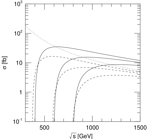
FIG. 1.: Production cross sections for $e^{+}e^{-}\to H^{+}H^{-}$ (solid) and $AH$ (dashed) for $m_{H^{\pm}}=200$, 300, and 400 GeV from left to right, and $Zh$ (dotted) for $m_{H^{\pm}}=200$ GeV. (The $Zh$ cross sections for $m_{H^{\pm}}=300$ and 400 GeV are virtually identical.) The 1–loop radiative correction given in Eqs. (6) and (8) has been included with $m_{\tilde{t}}=1$ TeV, and we have set $\tan\beta=5$; the dependence on $\tan\beta$ is very weak for $m_{H^{\pm}}\gtrsim 200$ GeV.

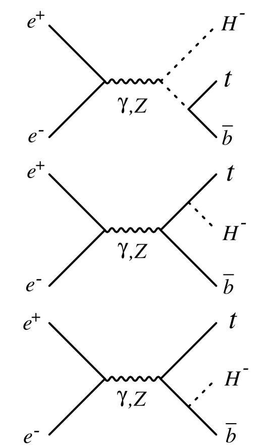
FIG. 2.: The three Feynman diagrams contributing to the three body final state $t\bar{b}H^{-}$. Three similar diagrams contribute to $\bar{t}bH^{+}$.

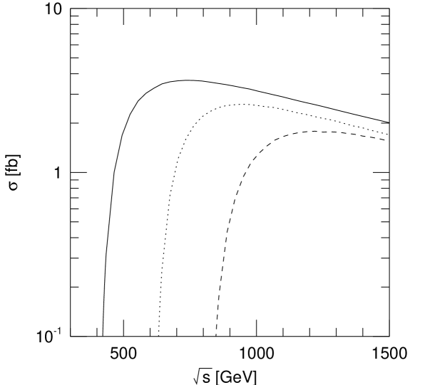
FIG. 3.: The three-body cross section $\sigma(e^{+}e^{-}\to t\bar{b}H^{-})+\sigma(e^{+}e^{-}\to\bar{t}bH^{+})$ for $m_{H^{\pm}}=200$ GeV (solid), 300 GeV (dotted), and 400 GeV (dashed), with $\tan\beta=60$. We require $E_{t}+E_{b}>1.02\sqrt{s}/2$ to separate this mode from the two-body production of $H^{+}H^{-}$ followed by $H^{\pm}\to tb$.

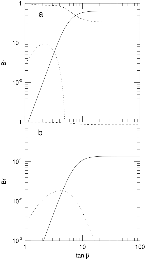
FIG. 4.: The branching ratios for $H^{-}$ to $\tau\bar{\nu}$ (solid), $\bar{t}b$ (dashed), and $W^{-}h$ (dotted) for (a) $m_{H^{\pm}}=200$ GeV and (b) $m_{H^{\pm}}=400$ GeV. The leading $m_{t}^{4}$ radiative correction of Eqs. (6) and (8) is included with $m_{\tilde{t}}=1$ TeV in calculating the remaining Higgs masses and mixings. The running quark mass $m_{b}=3.2$ GeV has been used, and all SUSY decay modes are assumed suppressed.

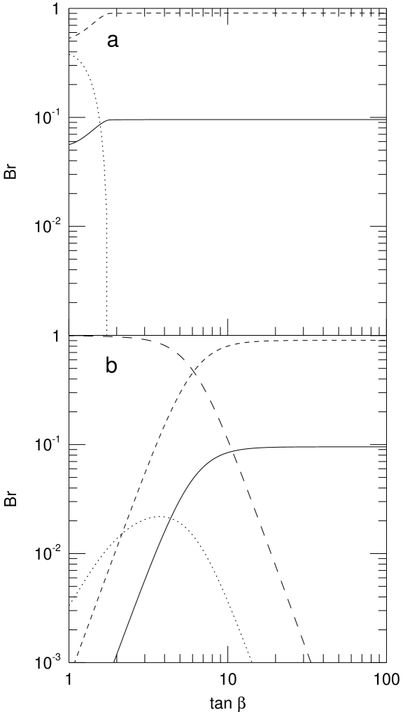
FIG. 5.: Same as in Fig. 4, but for CP–odd scalar $A$ decays to $\tau\bar{\tau}$ (solid), $b\bar{b}$ (short dash), $t\bar{t}$ (long dash), and $Zh$ (dotted).

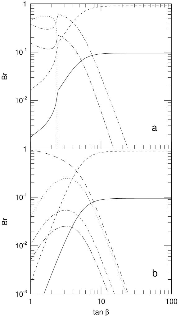
FIG. 6.: Same as in Fig. 4, but for neutral Higgs scalar $H$ decays to $\tau\bar{\tau}$ (solid), $b\bar{b}$ (short dash), $t\bar{t}$ (long dash), $hh$ (dotted), $W^{+}W^{-}$ (dot – short dash), and $ZZ$ (dot – long dash).

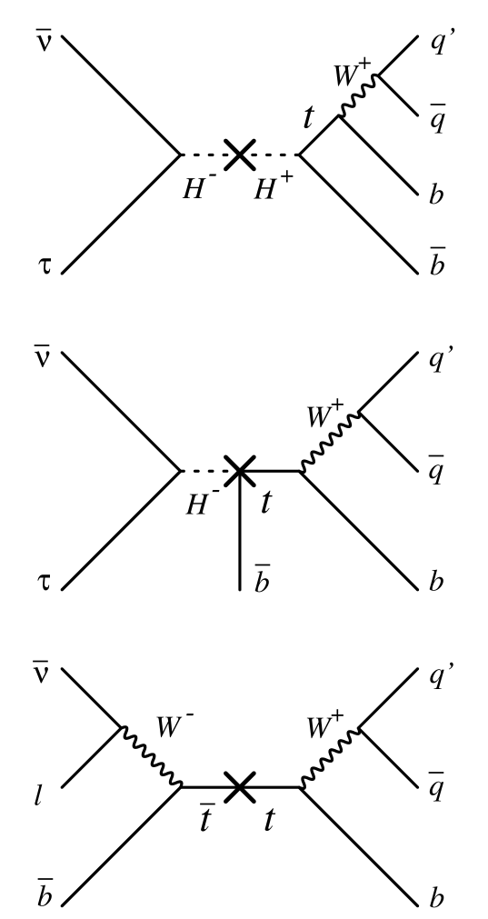
FIG. 7.: Schematic pictures of signal events $H^{+}H^{-}\to t\bar{b}\tau\bar{\nu}$ and $t\bar{b}H^{-}\to t\bar{b}\tau\bar{\nu}$, and background $t\bar{t}\to b\bar{q}q^{\prime}\bar{b}l\bar{\nu}$. The crosses mark the interaction point.

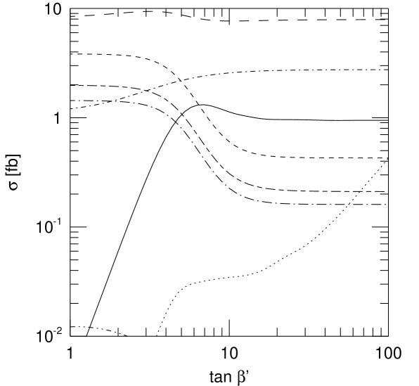
FIG. 8.: Signal cross sections for $m_{H^{\pm}}=200$ GeV, $\tan\beta=5$, and $\sqrt{s}=500$ GeV, in each channel: (1) $2b+l+q\text{'s}+\text{ cuts 1a--1e}$ (“$H^{+}H^{-}$” channel) (solid), (2) $2b+l+q\text{'s}+\text{ cuts 2a--2e}$ (“$tbH^{\pm}$” channel) (dotted), (3) $3b+1l\ (+q\text{'s})$ (short dash), (4) $3b+0,2,3,\ldots\ l\ (+q\text{'s})$ (long dash), (5) $4b$ (dot–short dash), 6) $4b+1l\ (+q\text{'s})$ (dot–long dash), (7) $4b+0,2,3,\ldots\ l\ (+q\text{'s})$ (but not $4b$) (short dash–long dash), and (8) $5b\ (+\ l+q\text{'s})$ (dash–dot–dot). All branching fractions, tagging efficiencies, and cuts have been included.

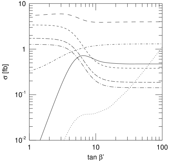
FIG. 9.: Signal cross sections as in Fig. 8, but for $m_{H^{\pm}}=200$ GeV and $\sqrt{s}=1$ TeV. The cross section for channel 8 is less than $10^{-2}\text{ fb}$, and therefore does not appear.

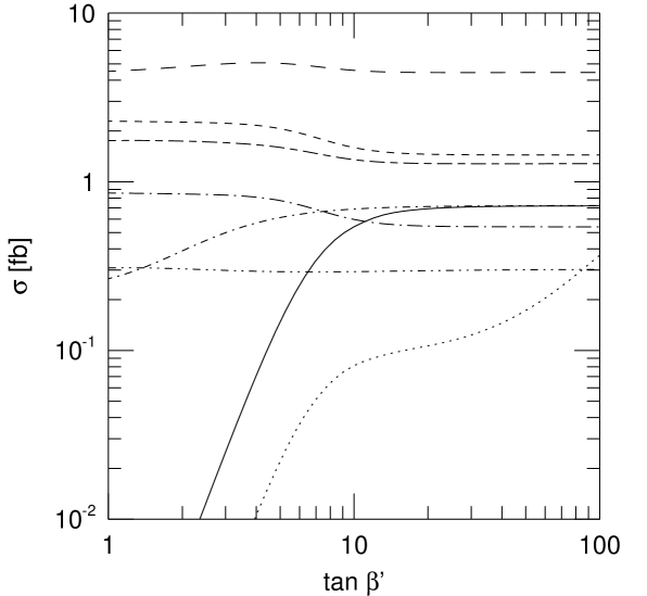
FIG. 10.: Signal cross sections as in Fig. 8, but for $m_{H^{\pm}}=300$ GeV and $\sqrt{s}=1$ TeV.

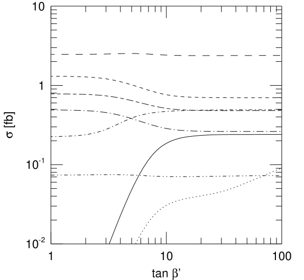
FIG. 11.: Signal cross sections as in Fig. 8, but for $m_{H^{\pm}}=400$ GeV and $\sqrt{s}=1$ TeV.

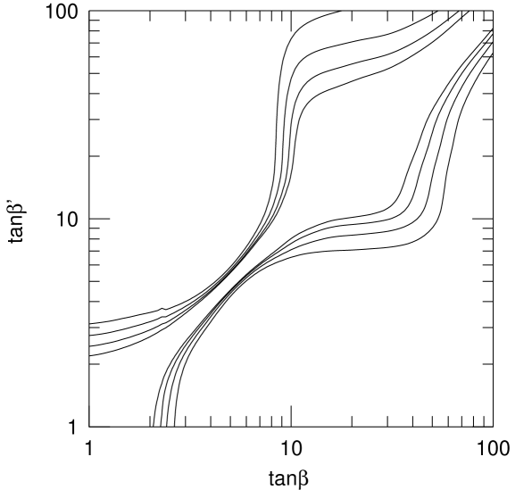
FIG. 12.: 95% C.L. bounds on $\tan\beta$ for $\sqrt{s}=500$ GeV, $m_{H^{\pm}}=200$ GeV, $\epsilon_{b}=60\%$, and four integrated luminosities: 25, 50, 100, and 200 fb^-1 (from outside to inside). For a fixed underlying value of $\tan\beta$, the values of $\tan\beta^{\prime}$ determined by the appropriate contours are the upper and lower bounds that may be set experimentally.

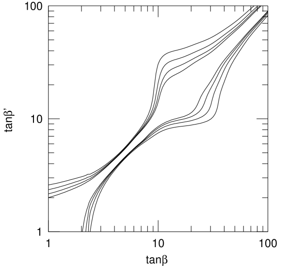
FIG. 13.: 95% C.L. bounds on $\tan\beta$ for $\sqrt{s}=1$ TeV, $m_{H^{\pm}}=200$ GeV, $\epsilon_{b}=60\%$, and four integrated luminosities: 100, 200, 400, and 800 fb^-1.

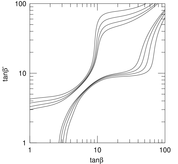
FIG. 14.: 95% C.L. bounds on $\tan\beta$ for $\sqrt{s}=1$ TeV, $m_{H^{\pm}}=300$ GeV, $\epsilon_{b}=60\%$, and four integrated luminosities: 100, 200, 400, and 800 fb^-1.

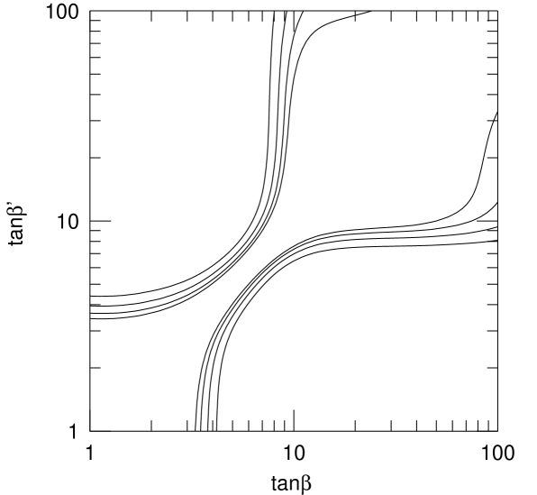
FIG. 15.: 95% C.L. bounds on $\tan\beta$ for $\sqrt{s}=1$ TeV, $m_{H^{\pm}}=400$ GeV, $\epsilon_{b}=60\%$, and four integrated luminosities: 100, 200, 400, and 800 fb^-1.

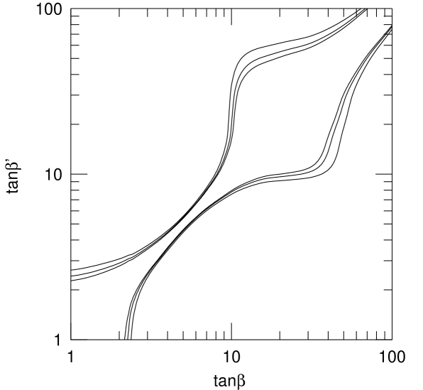
FIG. 16.: 95% C.L. bounds on $\tan\beta$ for $\sqrt{s}=500$ GeV, $m_{H^{\pm}}=200$ GeV, an integrated luminosity of 100 fb^-1, and $\epsilon_{b}=50$, 60, and 70% (from outside to inside).

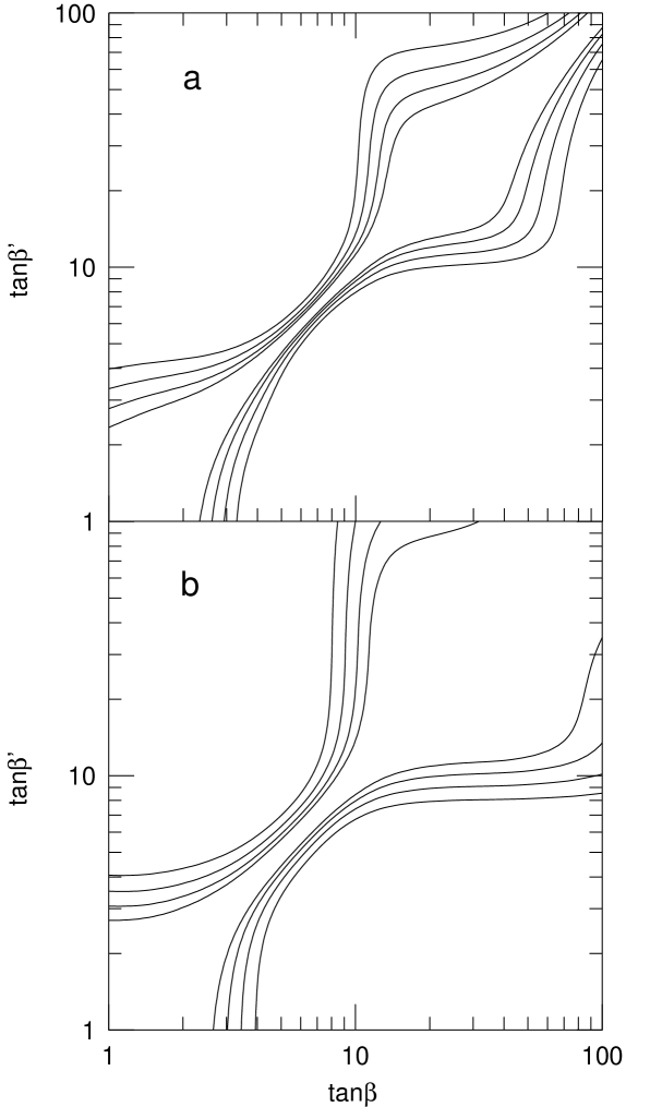
FIG. 17.: 95% C.L. bounds on $\tan\beta$ for (a) $m_{H^{\pm}}=300$ GeV and (b) $m_{H^{\pm}}=400$ GeV, $\sqrt{s}=1$ TeV, $\epsilon_{b}=60\%$, and four integrated luminosities: 100, 200, 400 and 800 fb^-1 with all systematic uncertainties omitted.

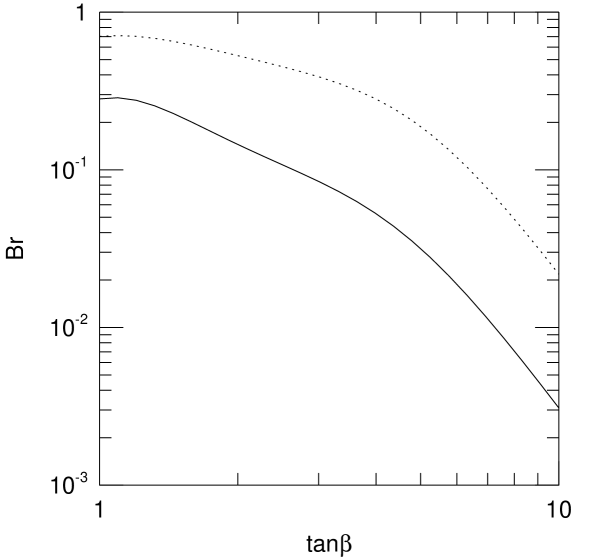
FIG. 18.: Branching ratios $B(H\to\tilde{l}_{R}^{*}\tilde{l}_{R})$ (solid) and $B(H\to\tilde{l}_{L}^{*}\tilde{l}_{L})+B(H\to\tilde{\nu}_{L}^{*}\tilde{\nu}_{L})$ (dashed). The $H$ mass and couplings are determined for fixed $m_{H^{\pm}}=300$ GeV, and include the radiative correction of Eqs. (6) and (8) with $m_{\tilde{t}}=1$ TeV. For the solid (dashed) curve, the three generations of right- (left-) handed sleptons are assumed degenerate with mass $m_{\tilde{l}_{R}}=100$ GeV ($m_{\tilde{l}_{L}}=100$ GeV), and all other sparticles decay modes are assumed closed.

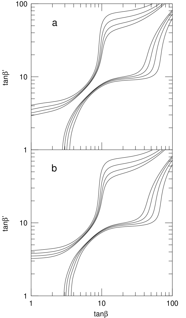
FIG. 19.: 95% C.L. bounds on $\tan\beta$ for $\sqrt{s}=1$ TeV, $m_{H^{\pm}}=300$ GeV, $\epsilon_{b}=60\%$, and four integrated luminosities: 100, 200, 400, and 800 fb^-1, with (a) only the right-handed slepton decays open with $m_{\tilde{l}_{R}}=100$, and (b) only the left-handed slepton decays open with $m_{\tilde{l}_{L}}=100$ GeV. All systematic errors are included.

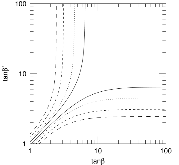
FIG. 20.: Contours of constant $\Delta m=$ 0.5 GeV (solid), 1 GeV (dotted), 2 GeV (short-dashed), and 3 GeV (long-dashed), where $\Delta m=\left|m_{\tilde{E}}(\tan\beta)-m_{\tilde{E}}(\tan\beta^{\prime})\right|$, for fixed physical mass $m_{\tilde{e}_{R}}=100$ GeV.

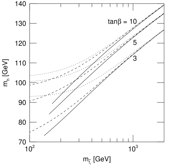
FIG. 21.: The lightest Higgs mass $m_{h}$ as a function of the mass of the lighter stop $m_{\tilde{t}_{1}}$ for $\tan\beta=3$, 5, and 10. Here, we fix $\mu=200\text{ GeV}$, $m_{A}=300$ GeV, and $A_{t}=0$ (solid lines), $A_{t}=200\text{ GeV}$ (dashed lines), and $A_{t}=-200\text{ GeV}$ (dotted lines).

REFERENCES

- [1] S. Kelly, J. L. Lopez, and D. V. Nanopoulos, Phys. Lett. B247, 387 (1992); V. Barger, M.S. Berger, and P. Ohmann, Phys. Rev. D 47, 1093 (1993); P. Langacker and N. Polonsky, Phys. Rev. D 49, 1454 (1994).
- [2] B. Ananthanarayan, G. Lazarides and Q. Shafi, Phys. Rev. D 44, 1613 (1991); L. J. Hall, R. Rattazzi, and U. Sarid, Phys. Rev. D 50, 7048 (1994).
- [3] See M. E. Peskin, in Proceedings of the Yukawa International Seminar (YKIS–95), Kyoto, Japan, 1995, edited by M. Bando, K. Inoue, and T. Kugo (Prog. Theor. Phys. Suppl., 123), p. 507, and references therein.
- [4] A. Djouadi, J. Kalinowski, P. Ohmann, and P. M. Zerwas, DESY–95–213, hep-ph/9605339; J. F. Gunion and J. Kelly, UCD–96–24, hep-ph/9610495.
- [5] NLC ZDR Design Group and the NLC Physics Working Group, S. Kuhlman et al., Physics and Technology of the Next Linear Collider, hep-ex/9605011.
- [6] The NLC Design Group, C. Adolphsen et al., Zeroth-Order Design Report for the Next Linear Collider, LBNL–PUB–5424, SLAC Report No. 474, UCRL–ID–124161 (1996).
- [7] JLC Group, JLC–I, KEK Report No. 92–16, Tsukuba (1992).
- [8] S. Komamiya, Phys. Rev. D 38, 2158 (1988).
- [9] J. F. Gunion, in Proceedings of the Workshop on Physics and Experiments with Linear Colliders, Waikoloa, Hawaii, 1993, edited by F.A. Harris, S.L. Olsen, S. Pakvasa, and X. Tata (World Scientific, Singapore, 1993), Vol. I, p. 166, hep-ph/9307367.
- [10] H. Murayama and M. E. Peskin, to be published in Ann. Rev. Nucl. Part. Sci., SLAC–PUB–7149, hep-ex/9606003, and references therein.
- [11] For a more complete review, see J. Gunion, H. E. Haber, G. Kane, and S. Dawson, The Higgs Hunter’s Guide (Addison-Wesley, Redwood City, California, 1990).
- [12] H. E. Haber and R. Hempfling, Phys. Rev. Lett. 66, 1815 (1991); Y. Okada, M. Yamaguchi, and T. Yanagida, Prog. Theor. Phys. 85, 1 (1991); J. Ellis, G. Ridolfi, and F. Zwirner, Phys. Lett. B257, 83 (1991); ibid, B262, 477 (1991).
- [13] A. Sopczak, Z. Phys. C 65, 449 (1995).
- [14] A. Djouadi, H. E. Haber, and P. M. Zerwas, Phys. Lett. B375, 203 (1996).
- [15] See, for example, M. Drees and M.M. Nojiri, Phys.Rev. D47, 376 (1993).
- [16] A. Djouadi, J. Kalinowski, P. M. Zerwas, Z. Phys. C 54, 255 (1992).
- [17] D. Jackson, talk given at Snowmass ’96, Colorado, June 25 – July 12, 1996.
- [18] V. D. Barger and P. J. Phillips, Collider Physics (Addison-Wesley, Redwood City, California, 1987).
- [19] H. Murayama, I. Watanabe, and K. Hagiwara, KEK Report No. 91–11, Tsukuba (1992).
- [20] S. Kawabata, Comp. Phys. Comm. 41, 127 (1986).
- [21] T. Tsukamoto, K. Fujii, H. Murayama, M. Yamaguchi, and Y. Okada, Phys. Rev. D 51, 3153 (1995).
- [22] H. Murayama, Ph.D. thesis, UT-580 (1991).
- [23] D. Jackson, private communication.
- [24] C. S. Li and J. M. Yang, Phys. Lett. B315, 367 (1993); H. Konig, Mod. Phys. Lett. A 10, 1113 (1995); A. Bartl, H. Eberl, K. Hidaka, T. Kon, W. Majerotto, and Y. Yamada, Phys. Lett. B378, 167 (1996); R. A. Jimenez and J. Sola, UAB–FT–376, hep-ph/9511292.
- [25] J. A. Coarasa, R. A. Jimenez, and J. Sola, UAB–FT–377, hep-ph/9511402.
- [26] A. Arhrib, M. C. Peyranere, and G. Moultaka, Phys. Lett. B341, 313 (1995); A. Arhrib and G. Moultaka, in Proceedings of Physics with Linear Colliders, Annecy, France, 1995, PM–96–16, hep-ph/9606300.
- [27] J. Gunion and H. Haber, Nucl. Phys. B278, 449 (1986); H. Baer, D. Dicus, M. Drees, and X. Tata, Phys. Rev. D 36, 1363 (1987); K. Griest and H. Haber, Phys. Rev. D 37, 719 (1988); H. Baer, M. Bisset, D. Dicus, C. Kao, and X. Tata, Phys. Rev. D 47, 1062 (1993); A. Djouadi, J. Kalinowski, P. M. Zerwas, Z. Phys. C 57, 569 (1993);
- [28] A. Bartl, H. Eberl, K. Hidaka, T. Kon, W. Majerotto, and Y. Yamada, UWTHPH–1996–44, hep-ph/9607388.
- [29] R. Becker and C. Vander Velde, in Proceedings of the Workshop on Physics and Experiments with Linear Colliders, Waikoloa, Hawaii, 1993, edited by F.A. Harris, S.L. Olsen, S. Pakvasa, and X. Tata (World Scientific, Singapore, 1993), Vol. II, p. 822.
- [30] M. M. Nojiri, K. Fujii, and T. Tsukamoto, Phys. Rev. D 54, 6756 (1996).
- [31] N. Arkani-Hamed, H.-C. Cheng, J. L. Feng, and L. J. Hall, Phys. Rev. Lett. 77, 1937 (1996); ibid., work in progress.
- [32] Y. Kawamura, H. Murayama, and M. Yamaguchi, Phys. Lett. B324, 52 (1994).
- [33] T. Moroi, Phys. Lett. B321, 56 (1994); R. Barbieri and L. J. Hall, Phys. Lett. B338, 212 (1994).
- [34] J. Feng and D. Finnell, Phys. Rev. D 49, 2369 (1994).
- [35] J. L. Feng and T. Moroi, in preparation.
- [36] J. L. Feng, H. Murayama, M. E. Peskin, and X. Tata, Phys. Rev. D 52, 1418 (1995).
- [37] T. Moroi, Phys. Rev. D 53, 6565 (1996).
- [38] CMS Collaboration, Technical Proposal, CERN/LHCC/94–38 (1994); ATLAS Collaboration, Technical Proposal, CERN/LHCC/94–43 (1994).
- [39] J. F. Gunion, A. Stange, and S. Willenbrock, to be published in Electroweak Symmetry Breaking and New Physics at the TeV Scale, edited by T. L. Barklow, S. Dawson, H. E. Haber, and J. L. Siegrist (World Scientific, Singapore, 1996), hep-ph/9602238.
- [40] I. Hinchliffe, F. E. Paige, M. D. Shapiro, J. Soderqvist, and W. Yao, LBNL–39412, hep-ph/9610544.
- [41] The NLC SUSY Subgroup, M. N. Danielson et al., to be published in Proceedings of the 1996 DPF/DPB Summer Study on New Directions for High Energy Physics (Snowmass ’96), Colorado, June 25 – July 12, 1996.