hep-ph/9612329

December 1996

Top-quark pole mass

Martin C. Smith and Scott S. Willenbrock

Department of Physics

University of Illinois

1110 West Green Street

Urbana, IL  61801

The top quark decays more quickly than the strong-interaction time scale, $\Lambda_{\rm QCD}^{-1}$, and might be expected to escape the effects of nonperturbative QCD. Nevertheless, the top-quark pole mass, like the mass of a stable heavy quark, is ambiguous by an amount proportional to $\Lambda_{\rm QCD}$.

1 Introduction

The mass of the recently-discovered top quark [1] has been measured with impressive accuracy, $m_{t}=175\pm 6$ GeV [2], by the CDF and D0 experiments at the Fermilab Tevatron. The uncertainty will be reduced even further, to perhaps 1-2 GeV, with additional running at the Tevatron [3], or at the CERN Large Hadron Collider [4]. High-energy $e^{+}e^{-}$ [5] or $\mu^{+}\mu^{-}$ [6] colliders operating at the $t\bar{t}$ threshold hold the promise of yet more precise measurements of $m_{t}$, to 200 MeV or even better.

With such increasingly-precise measurements on the horizon, it is important to have a firm grasp of exactly what is meant by the top-quark mass. Thus far the top-quark mass has been experimentally defined by the position of the peak in the invariant-mass distribution of the top-quark’s decay products, a $W$ boson and a $b$-quark jet [2]. This closely corresponds to the pole mass of the top quark, defined as the real part of the pole in the top-quark propagator. The propagator of a top quark with four-momentum $p$ has a pole at the complex position $\sqrt{p^{2}}=m_{pole}-\frac{i}{2}\Gamma$, and yields a peak in the $Wb$ invariant-mass distribution (for experimentally-accessible real values of $p$) when $\sqrt{p^{2}}\approx m_{pole}$.

The pole mass of a stable quark is well-defined in the context of finite-order perturbation theory [7]. However, the all-orders resummation of a certain class of diagrams, associated with “infrared renormalons”, indicates that the pole mass of a stable heavy quark is ambiguous by an amount proportional to $\Lambda_{\rm QCD}$, as a result of nonperturbative QCD [8, 9]. Physically, this is a satisfying result, because we believe that quarks are permanently confined within hadrons, precluding the unambiguous definition of a quark pole mass [10].

The top quark decays very quickly, having a width $\Gamma\approx{1.5\;{\rm GeV}}$, approximately an order of magnitude greater than the strong-interaction energy scale $\Lambda_{\rm QCD}\approx 200\;{\rm MeV}$. Such a short lifetime means that the top quark decays before it has time to hadronize [11, 12, 13]. The large top-quark width can act as an infrared cutoff, potentially insulating the top quark from the effects of nonperturbative QCD [14, 15, 16].

Given this information, one might expect the top-quark pole mass to be free of the ambiguities associated with nonperturbative QCD. The purpose of this article is to demonstrate that this is not the case. The top-quark pole mass, like the mass of a stable heavy quark, is unavoidably ambiguous by an amount proportional to $\Lambda_{\rm QCD}$. We demonstrate this in two ways, first by a general argument using $S$-matrix theory, second by a consideration of infrared renormalons. The ambiguity in the pole mass in the specific context of the $Wb$ invariant-mass distribution is discussed at the end of the next section.

2 General Argument

Consider a scattering process with asymptotic states consisting of stable particles. We first ask if it is possible for the scattering amplitude to have a pole at the mass of a stable quark. This would correspond to a quark propagator connecting two subamplitudes, as depicted in Fig. 1; the pole in the quark propagator would correspond to the pole in the amplitude. Such a configuration is impossible, however: the subamplitudes which the quark propagator connects have external states which are color singlets (due to confinement), while the quark is a color triplet, so color is not conserved. Thus there cannot be a pole in the amplitude at the quark mass.

Figure 1: A scattering amplitude factorizes when an internal propagator is near its pole. The external lines represent color-singlet asymptotic states.

This argument applies equally well to an unstable quark, such as the top quark. The fact that the quark is unstable evidently plays no role in the argument; it only shifts the imagined pole in the propagator into the complex plane. As in the case of a stable quark, there cannot be a pole in the amplitude, regardless of how short-lived the quark. In particular, the fact that the top-quark lifetime is much less than $\Lambda_{\rm QCD}^{-1}$ is irrelevant.

There is another way to understand why the short top-quark lifetime is irrelevant. Let us return to Fig. 1, and again consider first the case of a stable quark. Imagine that there is a pole in the amplitude at the quark mass. Near the pole, the scattering amplitude would factorize into the production of the stable quark by scattering subprocess A, followed by its propagation over a large proper time, and concluding with its participation in scattering subprocess B. Thus the quark could be considered as an asymptotic state. This demonstrates that the poles in the scattering amplitude of a theory correspond to its asymptotic states [17]. Since quarks are not asymptotic states, due to confinement, there cannot be a pole at the quark mass.

A similar argument applies to an unstable quark, such as the top quark. The imagined pole position is now located at a complex value. Because the scattering amplitude is an analytic function, the analytic continuation to complex momentum is well-defined. Near the pole, the scattering amplitude would factorize as before, although this would no longer correspond to a true physical process since the top-quark would have complex momentum [18]. The top quark would propagate over a large proper time, and could not escape confinement. There would be no asymptotic top-quark state, and hence no pole.

We are left with the following physical picture. A state with momentum near its pole corresponds to a long-lived particle, regardless of whether the pole is real or complex. If the particle is colored, it will be confined, preventing an unambiguous definition of the pole mass of the particle.

These arguments imply that the nonperturbative aspect of the strong interaction will stand in the way of any attempt to unambiguously extract the top-quark pole mass from experiment. For example, consider the extraction of the pole mass from the peak in the $Wb$ invariant-mass distribution. In perturbation theory, the final state is a $W$ and a $b$ quark, as depicted in Fig. 2(a). However, the $b$ quark manifests itself experimentally as a jet of colorless hadrons, due to confinement. At least one of the quarks which resides in these hadrons comes from elsewhere in the diagram, and cannot be considered as a decay product of the top quark, as depicted in Fig. 2(b). This leads to an irreducible uncertainty in the $Wb$ invariant mass of ${\sl O}(\Lambda_{\rm QCD})$, and hence an ambiguity of this amount in the extracted top-quark pole mass.

Figure 2: The production and decay of a top quark in (a) perturbation theory, and (b) nonperturbatively.

3 Infrared Renormalons

We now turn to an investigation of the top-quark pole mass from the perspective of infrared renormalons. We first review the argument which demonstrates the existence of a renormalon ambiguity in the pole mass of a stable heavy quark [8, 9]. We then extend the argument to take into account the finite width of the top quark. Finally, we investigate the existence of a renormalon ambiguity in the top-quark width itself.

The pole mass of a quark is defined by the position of the pole in the quark propagator. The propagator of a quark of four-momentum $p$ is

$$D(p\!\!\!/)=\frac{i}{p\!\!\!/-m_{R}-\Sigma(p\!\!\!/)}$$ (1)

where $m_{R}$ is a renormalized short-distance mass, and $\Sigma(p\!\!\!/)$ is the renormalized one-particle-irreducible quark self-energy. The equation for the position of the pole is

$$p\!\!\!/_{pole}=m_{R}+\Sigma(p\!\!\!/_{pole})\;.$$ (2)

This is an implicit equation for $p\!\!\!/_{pole}$ that can be solved perturbatively. We first work to leading order in $\alpha_{s}$, which gives

$$p\!\!\!/_{pole}=m_{R}+\Sigma^{(1)}(m_{R})$$ (3)

where $\Sigma^{(1)}(m_{R})$ is the one-loop quark self-energy shown Fig. 3(a). This quantity is real, so the pole position is real.

Figure 3: Diagrams contributing to the top-quark self-energy at leading order in $\alpha_{s}$ and $\alpha_{W}$. Fig. (a^′) replaces Fig. (a) when summing to all orders in $\beta_{0}\alpha_{s}$.

Renormalons arise from the class of diagrams generated by the insertion of $n$ vacuum-polarization subdiagrams into the gluon propagator in the one-loop self-energy diagram, as shown in Fig. 3(a^′). One can express this as

$$\Sigma^{(1)}(m_{R},a)=\frac{16m_{R}}{3\beta_{0}}\sum_{n=0}^{\infty}c_{n}a^{n+1}$$ (4)

where

$$a\equiv\frac{\beta_{0}\alpha_{s}(m_{R})}{4\pi}$$ (5)

and $\beta_{0}$ is the one-loop QCD beta-function coefficient, $\beta_{0}\equiv 11-(2/3)N_{f}$. Formally, these are the dominant QCD corrections in the “large-$\beta_{0}$” limit. Thus $\Sigma^{(1)}(m_{R},a)$ in Eq. (4) is calculated at leading order in $\alpha_{s}$, but to all orders in $a$.

For large $n$ the coefficients $c_{n}$ grow factorially, and are given by [19, 20, 21]

$$c_{n}\stackrel{{\scriptstyle n\to\infty}}{{\rightarrow}}e^{-C/2}2^{n}n!$$ (6)

where $C$ is a finite renormalization-scheme-dependent constant. The series in Eq. (4) is therefore divergent. One can attempt to sum the series using the technique of Borel resummation [22]. The Borel transform (with respect to $a$) of the self-energy is obtained from the series coefficients, Eq. (6), via

$$\widetilde{\Sigma}^{(1)}(m_{R},u)=\frac{16}{3\beta_{0}}m_{R}\sum_{n=0}^{\infty}\frac{c_{n}}{n!}\,u^{n}$$ (7)

where $u$ is the Borel parameter. Because the coefficients $c_{n}$ are divided by $n!$ in the above expression, the series has a finite radius of convergence in $u$, and can be analytically continued into the entire $u$ plane. The self-energy is then reconstructed via the inverse Borel transform, given formally by

$$\Sigma^{(1)}(m_{R},a)=\int_{0}^{\infty}du\,e^{-u/a}\widetilde{\Sigma}^{(1)}(m_{R},u)$$ (8)

The integral in Eq. (8) is only formal, because the Borel transform of the quark self-energy possesses singularities on the real $u$-axis, which impede the evaluation of the integral. These singularities are referred to as infrared renormalons because they arise from the region of soft gluon momentum in Fig. 3(a^′). The series for the self-energy in Eq. (4) is therefore not Borel summable.

The divergence of the series for the self-energy is governed by the infrared renormalon closest to the origin, which lies at $u=1/2$. This renormalon is not associated with the condensate of a local operator, so it cannot be absorbed into a nonperturbative redefinition of the pole mass [8, 9]. Instead, one can choose some ad hoc prescription to circumvent the singularity in the integral. The difference between various prescriptions is a measure of the ambiguity in the pole mass. Estimating the ambiguity as half the difference between deforming the integration contour above and below the singularity gives [9]

$$\delta m_{pole}\sim\frac{8\pi}{3\beta_{0}}e^{-C/2}\Lambda_{\rm QCD}$$ (9)

so the pole mass is ambiguous by an amount proportional to $\Lambda_{\rm QCD}$.

We now include the $O(\alpha_{W})$ contribution to the top-quark self-energy shown in Fig. 3(b). The pole position is still given by Eq. (3), but where $\Sigma^{(1)}(m_{R})$ includes both Figs. 3(a) and (b). Since Fig. 3(b) has an imaginary part, the pole moves off the real axis. The imaginary part of the one-loop pole position defines the tree-level top-quark width via ${\rm Im}\,\Sigma^{(1)}(m_{R})\equiv-\frac{1}{2}\Gamma_{tree}$. As before, to extend the calculation to all orders in $a$, we replace Fig. 3(a) by Fig. 3(a^′). This contribution to the pole mass remains the same as for a stable quark, and has the same renormalon ambiguity. At leading order in $\alpha_{W}$, the infrared renormalons do not know about the top-quark width.

The $O(\alpha_{s})$ contribution to the top-quark self-energy learns about the top-quark width if one works to all orders in $\alpha_{W}$, via a Schwinger-Dyson representation [23], as shown in Fig. 4. The circles on the internal propagators and the vertex in Figs. 4(a) and (b) represent the weak corrections to all orders in $\alpha_{W}$. We wish to solve for the pole position as given by Eq. (2). We denote the pole position at zeroth order in $\alpha_{s}$, but to all orders in $\alpha_{W}$, by the complex value $M$, with ${\rm Im}\,M\,\equiv-\frac{1}{2}\Gamma$, where $\Gamma$ is the top-quark width to all orders in $\alpha_{W}$. At leading order in $\alpha_{s}$, the pole position is then given by

$$p\!\!\!/_{pole}=m_{R}+\Sigma(M)$$ (10)

where $\Sigma(M)$ is given by Figs. 4(a) and (b). Again, we extend this calculation to all orders in $a$ by making $n$ vacuum-polarization insertions in the gluon propagator, as depicted in Fig 4(a^′). This yields a series in $a$, which we denote by $\Sigma(M,a)$ in analogy with Eq. (4). To investigate whether the width might cut off the infrared renormalons generated by these diagrams, we need only consider the contribution of soft gluons. In the limit of vanishing gluon momentum, the internal propagator reduces to $Z/(p\!\!\!/-M)$, where $Z$ is the wavefunction-renormalization factor. The Ward identity tells us that, in this same limit, the dressed vertex is simply $Z^{-1}$. Thus, in the infrared limit, $\Sigma(M,a)$ is formally identical to $\Sigma^{(1)}(m_{R},a)$ with $m_{R}$ replaced by $M$ everywhere. The infrared renormalons, which are associated with the Borel transform with respect to $a$, are unaffected. The width does not act as an cutoff for infrared renormalons, despite the fact that it is much greater than $\Lambda_{\rm QCD}$. We conclude that the pole mass of the top quark is ambiguous by an amount proportional to $\Lambda_{\rm QCD}$, just as for the case of a stable quark.

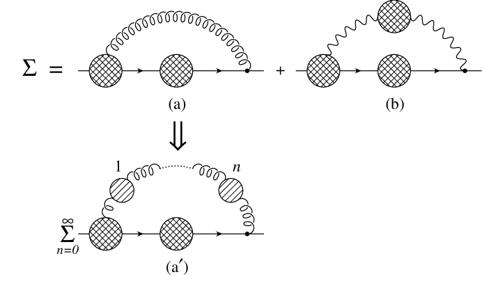
Figure 4: Diagrams contributing to the top-quark self energy at leading order in $\alpha_{s}$, but to all orders in $\alpha_{W}$. Fig. (a^′) replaces Fig. (a) when summing to all orders in $\beta_{0}\alpha_{s}$.

We next ask whether the top-quark width suffers from a similar renormalon ambiguity. Because the first-order calculation yields the top-quark width at tree level only, it is insufficient to address this question. The solution to Eq. (2) at $O(\alpha_{W}\alpha_{s})$ is

$$p\!\!\!/_{pole} = m_{R}+\Sigma(m_{R}+\Sigma(m_{R}))$$ (11)

$$= m_{R}+\Sigma^{(1)}(m_{R})+\Sigma^{(2)}(m_{R})+\Sigma^{(1)\prime}(m_{R})\Sigma^{(1)}(m_{R})$$

where the superscripts on $\Sigma$ indicate the order at which it is to be evaluated. The imaginary part of this equation (times $-1/2$) defines the top-quark width at $O(\alpha_{W}\alpha_{s})$.

One may calculate the imaginary part of Eq. (11) using the Cutkosky rules. This reduces to the calculation of the QCD correction to the process $t\to Wb$. The presence of renormalons in this process was investigated in Refs. [19, 20]. If the width is expressed in terms of the pole mass, then it has an infrared renormalon at $u=1/2$, corresponding to an ambiguity proportional to $\Lambda_{\rm QCD}$. However, if the width is expressed in terms of a short-distance mass, such as the $\overline{\rm MS}$ mass, there is no renormalon at $u=1/2$, and hence no ambiguity proportional to $\Lambda_{\rm QCD}$.

4 Conclusions

Although the top-quark lifetime is much less than the strong-interaction time scale, $\Lambda_{\rm QCD}^{-1}$, there are nonperturbative contributions to the top-quark pole mass, just as in the case of a stable heavy quark. These nonperturbative contributions are signaled by the divergent behavior at large orders of an expansion in $a=\beta_{0}\alpha_{s}(m_{R})/4\pi$. This leads to an unavoidable ambiguity of $O(\Lambda_{\rm QCD})$ in the pole mass of the top quark.

A short-distance mass, such as the $\overline{\rm MS}$ mass, can in principle be measured with arbitrary accuracy. This may require nonperturbative information, depending on the measurement. It is sensible to adopt the $\overline{\rm MS}$ mass as the standard definition of the top-quark mass, as is the convention for the lighter quarks [24]. The relation between the top-quark pole mass and the $\overline{\rm MS}$ mass evaluated at the pole mass, $\overline{m}(m_{pole})$, is known to two loops [25]:

$$m_{pole}=\overline{m}(m_{pole})\left(1+\frac{4}{3}\frac{\overline{\alpha}_{s}(m_{pole})}{\pi}+10.95\left(\frac{\overline{\alpha}_{s}(m_{pole})}{\pi}\right)^{2}+\cdots\right)+O(\Lambda_{\rm QCD})$$ (12)

where the last term reminds us that the pole mass has an unavoidable ambiguity of $O(\Lambda_{\rm QCD})$. Given that the pole mass is ambiguous, we suggest as the standard the $\overline{\rm MS}$ mass evaluated at the $\overline{\rm MS}$ mass, which is related to the pole mass by

$$m_{pole}=\overline{m}(\overline{m})\left(1+\frac{4}{3}\frac{\overline{\alpha}_{s}(\overline{m})}{\pi}+8.28\left(\frac{\overline{\alpha}_{s}(\overline{m})}{\pi}\right)^{2}+\cdots\right)+O(\Lambda_{\rm QCD})\;.$$ (13)

The difference in the coefficients of the two ${\overline{\alpha}_{s}}^{2}$ terms above is exactly 8/3. For a top-quark pole mass of $175\pm 6$ GeV, $\overline{m}(\overline{m})=166\pm 6$ GeV.

The considerations of this paper apply to any colored particle, stable or unstable. Thus, if nature is supersymmetric, the pole masses of squarks and gluinos will necessarily be ambiguous by an amount proportional to $\Lambda_{\rm QCD}$.

References

- [1] CDF Collaboration, F. Abe et al., Phys. Rev. Lett. 74, 2626 (1995); D0 Collaboration, S. Abachi et al., Phys. Rev. Lett. 74, 2632 (1995).
- [2] P. Tipton, presented at the XXVIII International Conference on High-Energy Physics, Warsaw, Poland, July 1996.
- [3] Future Electroweak Physics at the Fermilab Tevatron: Report of the tev_2000 Study Group, eds. D. Amidei and R. Brock, FERMILAB-Pub-96/082 (1996).
- [4] ATLAS Technical Proposal, CERN/LHCC/94-43, LHCC/P2 (1994).
- [5] Physics and Technology of the Next Linear Collider, NLC ZDR Design Group and the NLC Physics Working Group, hep-ex/9605011.
- [6] Collider: A Feasibility Study, Collider Collaboration, BNL-52503 (1996).
- [7] R. Tarrach, Nucl. Phys. B183, 384 (1981).
- [8] I. Bigi, M. Shifman, N. Uraltsev, and A. Vainshtein, Phys. Rev. D 50, 2234 (1994).
- [9] M. Beneke and V. Braun, Nucl. Phys. B426, 301 (1994).
- [10] I. Bigi and N. Uraltsev, Phys. Lett. B321, 412 (1994).
- [11] J. Kühn, Ann. Phys. Austr., Suppl. XXIV, 203 (1982).
- [12] I. Bigi, Y. Dokshitzer, V. Khoze, J. Kühn, and P. Zerwas, Phys. Lett. B181, 157 (1986).
- [13] L. Orr and J. Rosner, Phys. Lett. B246, 221 (1990); L. Orr, Phys. Rev. D 44, 88 (1991).
- [14] V. Fadin and V. Khoze, Pis’ma Zh. Eksp. Teoor. Fiz. 46, 417 (1987) [JETP Lett. 46, 525 (1987)]; Yad. Fiz. 48, 487 (1988) [Sov. J. Nucl. Phys., 48, 309 (1988)]; V. Fadin, V. Khoze, and T. Sjöstrand, Z. Phys. C 48, 613 (1990).
- [15] M. Strassler and M. Peskin, Phys. Rev. D 43, 1500 (1995).
- [16] V. Khoze and T. Sjöstrand, Phys. Lett. B328, 466 (1994).
- [17] R. Eden, P. Landshoff, D. Olive, and J. Polkinghorne, The Analytic S-Matrix (Cambridge University Press, Cambridge, 1966), section 4.5.
- [18] Ref. [17], section 4.9.
- [19] M. Beneke and V. Braun, Phys. Lett. B348, 513 (1995).
- [20] P. Ball, M. Beneke, and V. Braun, Nucl. Phys. B452, 563 (1995).
- [21] K. Philippides and A. Sirlin, Nucl. Phys. B450, 3 (1995).
- [22] G. ’t Hooft, in The Whys of Subnuclear Physics, Proceedings of the International School of Subnuclear Physics, Erice, 1977, ed. A. Zichichi (Plenum, New York, 1979), p. 943; A. Mueller, in QCD - 20 Years Later, Proceedings of the Workshop, Aachen, Germany, 1992, eds. P. Zerwas and H. Kastrup (World Scientific, Singapore, 1993), Vol. 1, p. 162.
- [23] Itzykson and Zuber, Quantum Field Theory (McGraw-Hill, New York, 1980), p. 475.
- [24] Review of Particle Properties, Phys. Rev. D 54, 1 (1996), p. 303.
- [25] N. Gray, D. Broadhurst, W. Grafe, and K. Schilcher, Z. Phys. C 48, 673 (1990).