ZU-TH 24/96
TUM-HEP-263/96
MPI/PhT/96-123
hep-ph/9612313
December 1996

Weak Radiative B-Meson Decay Beyond Leading Logarithms

Konstantin Chetyrkin${}^{{}^{1,\dagger}}$, Mikołaj Misiak${}^{{}^{2,\ddagger}}$ and Manfred Münz${}^{{}^{3}}$

${}^{{}^{1}}$Max-Planck-Institut für Physik, Werner-Heisenberg-Institut,
D-80805 München, Germany

${}^{{}^{2}}$Institut für Theoretische Physik der Universität Zürich,
CH-8057 Zürich, Switzerland

${}^{{}^{3}}$Physik Department, Technische Universität München,
D-85748 Garching, Germany

Abstract

We present our results for three-loop anomalous dimensions necessary in analyzing $B{\to}X_{s}\gamma$ decay at the next-to-leading order in QCD. We combine them with other recently calculated contributions, obtaining a practically complete next-to-leading order prediction for the branching ratio ${\cal B}(B{\to}X_{s}\gamma)=(3.28\pm 0.33)\times 10^{-4}$. The uncertainty is more than twice smaller than in the previously available leading order theoretical result. The Standard Model prediction remains in agreement with the CLEO measurement at the $2\sigma$ level.

                                            
¹ This work was partially supported by INTAS under Contract INTAS-93-0744.
² Supported in part by Schweizerischer Nationalfonds and Polish Commitee for Scientific Research (grant
2 P03B 180 09, 1995-97).
³ Supported in part by Deutsches Bundesministerium für Bildung und Forschung under contract 06 TM 743.
^† Permanent address: Institute of Nuclear Research, Russian Academy of Sciences, Moscow 117312, Russia. ^‡ Permanent address: Institute of Theoretical Physics, Warsaw University, Hoża 69, 00-681 Warsaw, Poland.

1. Weak radiative B-meson decay is known to be a very sensitive probe of new physics [1, 2]. Heavy Quark Effective Theory tells us that inclusive $B$-meson decay rate into charmless hadrons and the photon is well approximated by the corresponding partonic decay rate

$$\Gamma(B{\to}X_{s}\gamma)\simeq\Gamma(b{\to}X_{s}\gamma).$$ (1)

The accuracy of this approximation is expected to be better than 10% [3].

The inclusive branching ratio ${\cal B}(b{\to}X_{s}\gamma)$ was extracted two years ago from CLEO measurements of weak radiative $B$-meson decay. It amounts to [4]

$${\cal B}(b{\to}X_{s}\gamma)=(2.32\pm 0.57\pm 0.35)\times 10^{-4}.$$ (2)

In the forthcoming few years, much more precise measurements of ${\cal B}(B{\to}X_{s}\gamma)$ are expected from the upgraded CLEO detector, as well as from the B-factories at SLAC and KEK. Acquiring experimental accuracy of below 10% is conceivable. Thus, the goal on the theoretical side is to reach the same accuracy in perturbative calculations of $b{\to}X_{s}\gamma$ decay rate. This requires performing a complete calculation at the next-to-leading order (NLO) in QCD [1, 5]. All the next-to-leading contributions to $b{\to}X_{s}\gamma$ are collected for the first time in the present letter.

One of the most complex ingredients of the NLO calculation consists in finding three-loop anomalous dimensions in the effective theory used for resummation of large logarithms $\;\ln(M_{W}^{2}/m_{b}^{2})$. This is the main new result presented in this letter. However, we have recalculated all the previously found anomalous dimensions, too.

The remaining ingredients of the NLO calculation are already present in the literature [6]–[17]. We use the published results for the two-loop matrix elements calculated by Greub, Hurth and Wyler [9], Bremsstrahlung corrections obtained by Ali, Greub [15, 16] and Pott [17], and the matching conditions found by Adel and Yao [13].

The following three sections of the present paper are devoted to presenting the complete NLO formulae for $b{\to}X_{s}\gamma$. Next, we analyze them numerically. In the end, we discuss predictions for the branching ratio ${\cal B}(B{\to}X_{s}\gamma)$ including a discussion of the relevant uncertainties.

2. The analysis of $b{\to}X_{s}\gamma$ decay begins with introducing an effective hamiltonian

$$H_{eff}=-\frac{4G_{F}}{\sqrt{2}}V^{*}_{ts}V_{tb}\sum_{i=1}^{8}C_{i}(\mu)P_{i}(\mu)$$ (3)

where $V_{ij}$ are elements of the CKM matrix, $P_{i}(\mu)$ are the relevant operators and $C_{i}(\mu)$ are the corresponding Wilson coefficients. The complete set of physical operators necessary for $b{\to}X_{s}\gamma$ decay is the following:

$$\begin{array}[]{rl}P_{1}=&(\bar{s}_{L}\gamma_{\mu}T^{a}c_{L})(\bar{c}_{L}\gamma^{\mu}T^{a}b_{L})\vspace{0.2cm}\\ P_{2}=&(\bar{s}_{L}\gamma_{\mu}c_{L})(\bar{c}_{L}\gamma^{\mu}b_{L})\vspace{0.2cm}\\ P_{3}=&(\bar{s}_{L}\gamma_{\mu}b_{L})\sum_{q}(\bar{q}\gamma^{\mu}q)\vspace{0.2cm}\\ P_{4}=&(\bar{s}_{L}\gamma_{\mu}T^{a}b_{L})\sum_{q}(\bar{q}\gamma^{\mu}T^{a}q)\vspace{0.2cm}\\ P_{5}=&(\bar{s}_{L}\gamma_{\mu_{1}}\gamma_{\mu_{2}}\gamma_{\mu_{3}}b_{L})\sum_{q}(\bar{q}\gamma^{\mu_{1}}\gamma^{\mu_{2}}\gamma^{\mu_{3}}q)\vspace{0.2cm}\\ P_{6}=&(\bar{s}_{L}\gamma_{\mu_{1}}\gamma_{\mu_{2}}\gamma_{\mu_{3}}T^{a}b_{L})\sum_{q}(\bar{q}\gamma^{\mu_{1}}\gamma^{\mu_{2}}\gamma^{\mu_{3}}T^{a}q)\vspace{0.2cm}\\ P_{7}=&\frac{e}{16\pi^{2}}m_{b}(\bar{s}_{L}\sigma^{\mu\nu}b_{R})F_{\mu\nu}\vspace{0.2cm}\\ P_{8}=&\frac{g}{16\pi^{2}}m_{b}(\bar{s}_{L}\sigma^{\mu\nu}T^{a}b_{R})G_{\mu\nu}^{a}\end{array}$$ (4)

where $T^{a}$ stand for $SU(3)_{\rm color}$ generators. The small CKM matrix element $V_{ub}$ as well as the $s$-quark mass are neglected in the present paper.

Our basis of four-quark operators is somewhat different than the standard one used in refs. [1, 6, 18], although the two bases are physically equivalent. We would like to stress that in our basis, Dirac traces containing $\gamma_{5}$ do not arise in effective theory calculations performed at the leading order in the Fermi coupling $G_{F}$ (but to all orders in QCD). This allows us to consistently use fully anticommuting $\gamma_{5}$ in dimensional regularization, which greatly simplifies multiloop calculations. Our choice of color structures is dictated only by convenience in computer algebra applications.

Throughout the paper, we use the $\overline{MS}$ scheme with fully anticommuting $\gamma_{5}$. Such a scheme is not uniquely defined until one chooses a specific form for the so-called evanescent operators which algebraically vanish in four dimensions [19, 20]. In our three-loop calculation, eight evanescent operators were necessary. We list them explicitly in Appendix A.

Resummation of large logarithms $\ln(M_{W}^{2}/m_{b}^{2})$ is achieved by evolving the coefficients $C_{i}(\mu)$ from $\mu=M_{W}$ to $\mu=\mu_{b}\simeq m_{b}$ according to the Renormalization Group Equations (RGE). Instead of the original coefficients $C_{i}(\mu)$, it is convenient to use certain linear combinations of them, called the “effective coefficients” [1, 9]

$$C_{i}^{eff}(\mu)=\left\{\begin{array}[]{cc}C_{i}(\mu)&\mbox{ for $i=1,...,6$}\\ C_{7}(\mu)+\sum_{i=1}^{6}y_{i}C_{i}(\mu)&\mbox{ for $i=7$}\\ C_{8}(\mu)+\sum_{i=1}^{6}z_{i}C_{i}(\mu)&\mbox{ for $i=8$.}\end{array}\right.$$ (5)

The numbers $y_{i}$ and $z_{i}$ are defined so that the leading-order $b\to s\gamma$ and $b\to s\;gluon$ matrix elements of the effective hamiltonian are proportional to the leading-order terms in $C_{7}^{eff}$ and $C_{8}^{eff}$, respectively [1]. In the $\overline{MS}$ scheme with fully anticommuting $\gamma_{5}$, we have $y=(0,0,-\frac{1}{3},-\frac{4}{9},-\frac{20}{3},-\frac{80}{9})$ and $z=(0,0,1,-\frac{1}{6},20,-\frac{10}{3})$. The leading-order contributions to the effective coefficients $C_{i}^{eff}(\mu)$ are regularization- and renormalization-scheme independent, which would not be true for the original coefficients $C_{7}(\mu)$ and $C_{8}(\mu)$.

The effective coefficients evolve according to their RGE

$$\mu\frac{d}{d\mu}C_{i}^{eff}(\mu)=C_{j}^{eff}(\mu)\gamma^{eff}_{ji}(\mu)$$ (6)

driven by the anomalous dimension matrix $\hat{\gamma}^{eff}(\mu)$. One expands this matrix perturbatively as follows:

$$\hat{\gamma}^{eff}(\mu)=\frac{\alpha_{s}(\mu)}{4\pi}\hat{\gamma}^{(0)eff}+\frac{\alpha_{s}^{2}(\mu)}{(4\pi)^{2}}\hat{\gamma}^{(1)eff}+...$$ (7)

The matrix $\hat{\gamma}^{(0)eff}$ is renormalization-scheme independent, while $\hat{\gamma}^{(1)eff}$ is not. In the $\overline{MS}$ scheme with fully anticommuting $\gamma_{5}$ (and with our choice of evanescent operators) we obtain

$$\hat{\gamma}^{(0)eff}=\left[\begin{array}[]{cccccccc}\vspace{0.2cm}-4&\frac{8}{3}&0&-\frac{2}{9}&0&0&-\frac{208}{243}&\frac{173}{162}\\ \vspace{0.2cm}12&0&0&\frac{4}{3}&0&0&\frac{416}{81}&\frac{70}{27}\\ \vspace{0.2cm}0&0&0&-\frac{52}{3}&0&2&-\frac{176}{81}&\frac{14}{27}\\ \vspace{0.2cm}0&0&-\frac{40}{9}&-\frac{100}{9}&\frac{4}{9}&\frac{5}{6}&-\frac{152}{243}&-\frac{587}{162}\\ \vspace{0.2cm}0&0&0&-\frac{256}{3}&0&20&-\frac{6272}{81}&\frac{6596}{27}\\ \vspace{0.2cm}0&0&-\frac{256}{9}&\frac{56}{9}&\frac{40}{9}&-\frac{2}{3}&\frac{4624}{243}&\frac{4772}{81}\\ \vspace{0.2cm}0&0&0&0&0&0&\frac{32}{3}&0\\ \vspace{0.2cm}0&0&0&0&0&0&-\frac{32}{9}&\frac{28}{3}\\ \end{array}\right]$$ (8)

and

$$\hat{\gamma}^{(1)eff}=\left[\begin{array}[]{cccccccc}\vspace{0.2cm}-\frac{355}{9}&-\frac{502}{27}&-\frac{1412}{243}&-\frac{1369}{243}&\frac{134}{243}&-\frac{35}{162}&-\frac{818}{243}&\frac{3779}{324}\\ \vspace{0.2cm}-\frac{35}{3}&-\frac{28}{3}&-\frac{416}{81}&\frac{1280}{81}&\frac{56}{81}&\frac{35}{27}&\frac{508}{81}&\frac{1841}{108}\\ \vspace{0.2cm}0&0&-\frac{4468}{81}&-\frac{31469}{81}&\frac{400}{81}&\frac{3373}{108}&\frac{22348}{243}&\frac{10178}{81}\\ \vspace{0.2cm}0&0&-\frac{8158}{243}&-\frac{59399}{243}&\frac{269}{486}&\frac{12899}{648}&-\frac{17584}{243}&-\frac{172471}{648}\\ \vspace{0.2cm}0&0&-\frac{251680}{81}&-\frac{128648}{81}&\frac{23836}{81}&\frac{6106}{27}&\frac{1183696}{729}&\frac{2901296}{243}\\ \vspace{0.2cm}0&0&\frac{58640}{243}&-\frac{26348}{243}&-\frac{14324}{243}&-\frac{2551}{162}&\frac{2480344}{2187}&-\frac{3296257}{729}\\ \vspace{0.2cm}0&0&0&0&0&0&\frac{4688}{27}&0\\ \vspace{0.2cm}0&0&0&0&0&0&-\frac{2192}{81}&\frac{4063}{27}\\ \end{array}\right].$$ (9)

The matrix $\hat{\gamma}^{(1)eff}$ is the main new result of this paper. Its evaluation required performing three-loop renormalization of the effective theory (3). Details of this calculation will be given in a forthcoming publication [21].

We expand the coefficients in powers of $\alpha_{s}$ as follows:

$$C^{eff}_{i}(\mu)=C^{(0)eff}_{i}(\mu)+\frac{\alpha_{s}(\mu)}{4\pi}C^{(1)eff}_{i}(\mu)+...$$ (10)

At $\mu=M_{W}$, the values of the coefficients are found by matching the effective theory amplitudes with the full Standard Model ones. The well-known leading-order results read [1, 6, 22]

$$C_{i}^{(0)eff}(M_{W})=C_{i}^{(0)}(M_{W})=\left\{\begin{array}[]{cc}0&\mbox{ for $i=1,3,4,5,6$}\\ 1&\mbox{ for $i=2$}\\ \vspace{0.2cm}\frac{3x^{3}-2x^{2}}{4(x-1)^{4}}\ln x+\frac{-8x^{3}-5x^{2}+7x}{24(x-1)^{3}}&\mbox{ for $i=7$}\\ \frac{-3x^{2}}{4(x-1)^{4}}\ln x+\frac{-x^{3}+5x^{2}+2x}{8(x-1)^{3}}&\mbox{ for $i=8$},\\ \end{array}\right.$$ (11)

where

$$x=\frac{m_{t,\overline{MS}}^{2}(M_{W})}{M_{W}^{2}}=\frac{m_{t,pole}^{2}}{M_{W}^{2}}\left(\frac{\alpha_{s}(M_{W})}{\alpha_{s}(m_{t})}\right)^{\frac{24}{23}}\left(1-\frac{8}{3}\frac{\alpha_{s}(m_{t})}{\pi}\right).$$ (12)

The next-to-leading contributions to the four-quark operator coefficients at $\mu=M_{W}$ can be found either by transforming the results of ref. [10] to our operator basis, or by a direct computation. We find

$$C_{i}^{(1)eff}(M_{W})=C_{i}^{(1)}(M_{W})=\left\{\begin{array}[]{cc}15&\mbox{ for $i=1$}\\ 0&\mbox{ for $i=2,3,5,6$}\\ E(x)-\frac{2}{3}&\mbox{ for $i=4$},\end{array}\right.$$ (13)

where

$$E(x)=\frac{x(18-11x-x^{2})}{12(1-x)^{3}}+\frac{x^{2}(15-16x+4x^{2})}{6(1-x)^{4}}\ln x-\frac{2}{3}\ln x.$$ (14)

The next-to-leading contributions to $C_{7}^{eff}(M_{W})$ and $C_{8}^{eff}(M_{W})$ can be extracted from ref. [13] according to the following equations:

$$C_{7}^{(1)eff}(M_{W})=-8/3\frac{\pi}{4\alpha_{s}}\bar{C}^{(1)}_{O_{52}}+\Delta_{7}-\frac{4}{9}\left(E(x)-\frac{2}{3}\right),$$ (15)

$$C_{8}^{(1)eff}(M_{W})=8\frac{\pi}{4\alpha_{s}}\bar{C}^{(1)}_{O_{51}}+\Delta_{8}-\frac{1}{6}\left(E(x)-\frac{2}{3}\right),$$ (16)

where the quantities $\bar{C}^{(1)}_{O_{51}}$ and $\bar{C}^{(1)}_{O_{52}}$ are given in eqn. (5) of ref. [13] with $\mu=M_{W}$. The terms denoted by $\Delta_{7}$ and $\Delta_{8}$ stand for shifts one needs to make when passing from the so-called $R^{*}$ renormalization scheme used in ref. [13] to the $\overline{MS}$ scheme used here

$$\Delta_{i}=\frac{4\pi}{\alpha_{s}}\left[C_{i}^{(0)}(M_{W})(x\to x-\frac{2\alpha_{s}}{\pi}x\ln x)-C_{i}^{(0)}(M_{W})(x)\right]\hskip 28.45274pt\mbox{ for $i=7,8$}.$$ (17)

Only the leading (zeroth-order) term in $\alpha_{s}$ needs to be retained in the above equation.

The resulting explicit expressions for $C_{7}^{eff}(M_{W})$ and $C_{8}^{eff}(M_{W})$ in the $\overline{MS}$ scheme read

$$C_{7}^{(1)eff}(M_{W}) = \frac{-16x^{4}-122x^{3}+80x^{2}-8x}{9(x-1)^{4}}{\rm Li}_{2}\left(1-\frac{1}{x}\right)+\frac{6x^{4}+46x^{3}-28x^{2}}{3(x-1)^{5}}\ln^{2}x$$ (18)

$$+\frac{-102x^{5}-588x^{4}-2262x^{3}+3244x^{2}-1364x+208}{81(x-1)^{5}}\ln x$$

$$+\frac{1646x^{4}+12205x^{3}-10740x^{2}+2509x-436}{486(x-1)^{4}}\vspace{0.2cm}$$

$$C_{8}^{(1)eff}(M_{W}) = \frac{-4x^{4}+40x^{3}+41x^{2}+x}{6(x-1)^{4}}{\rm Li}_{2}\left(1-\frac{1}{x}\right)+\frac{-17x^{3}-31x^{2}}{2(x-1)^{5}}\ln^{2}x$$ (19)

$$+\frac{-210x^{5}+1086x^{4}+4893x^{3}+2857x^{2}-1994x+280}{216(x-1)^{5}}\ln x$$

$$+\frac{737x^{4}-14102x^{3}-28209x^{2}+610x-508}{1296(x-1)^{4}}$$

Having specified the initial conditions at $\mu=M_{W}$, we are ready to write the solution to the Renormalization Group Equations (6) for $C^{eff}_{7}(\mu_{b})$

$$C^{(0)eff}_{7}(\mu_{b})=\eta^{\frac{16}{23}}C^{(0)}_{7}(M_{W})+\frac{8}{3}\left(\eta^{\frac{14}{23}}-\eta^{\frac{16}{23}}\right)C^{(0)}_{8}(M_{W})+\sum_{i=1}^{8}h_{i}\eta^{a_{i}},$$ (20)

$$C^{(1)eff}_{7}(\mu_{b}) = \eta^{\frac{39}{23}}C^{(1)eff}_{7}(M_{W})+\frac{8}{3}\left(\eta^{\frac{37}{23}}-\eta^{\frac{39}{23}}\right)C^{(1)eff}_{8}(M_{W})$$ (21)

$$+\left(\frac{297664}{14283}\eta^{\frac{16}{23}}-\frac{7164416}{357075}\eta^{\frac{14}{23}}+\frac{256868}{14283}\eta^{\frac{37}{23}}-\frac{6698884}{357075}\eta^{\frac{39}{23}}\right)C_{8}^{(0)}(M_{W})$$

$$+\frac{37208}{4761}\left(\eta^{\frac{39}{23}}-\eta^{\frac{16}{23}}\right)C_{7}^{(0)}(M_{W})+\sum_{i=1}^{8}(e_{i}\eta E(x)+f_{i}+g_{i}\eta)\eta^{a_{i}},$$

where $\eta=\alpha_{s}(M_{W})/\alpha_{s}(\mu_{b})$, and the numbers $a_{i}$–$h_{i}$ are as follows

$$\begin{array}[]{ccccccccc}\vspace{0.2cm}a_{i}=(&\frac{14}{23},&\frac{16}{23},&\frac{6}{23},&-\frac{12}{23},&0.4086,&-0.4230,&-0.8994,&0.1456)\\ \vspace{0.2cm}e_{i}=(&\frac{4661194}{816831},&-\frac{8516}{2217},&0,&0,&-1.9043,&-0.1008,&0.1216,&0.0183)\\ \vspace{0.2cm}f_{i}=(&-17.3023,&8.5027,&4.5508,&0.7519,&2.0040,&0.7476,&-0.5385,&0.0914)\\ \vspace{0.2cm}g_{i}=(&14.8088,&-10.8090,&-0.8740,&0.4218,&-2.9347,&0.3971,&0.1600,&0.0225)\\ \vspace{0.2cm}h_{i}=(&\frac{626126}{272277},&-\frac{56281}{51730},&-\frac{3}{7},&-\frac{1}{14},&-0.6494,&-0.0380,&-0.0186,&-0.0057).\end{array}$$ (27)

As far as the other Wilson coefficients are concerned, only the leading-order contributions to them are necessary in the complete NLO analysis of $b{\to}X_{s}\gamma$. We obtain

$$\begin{array}[]{ccc}\vspace{0.2cm}C^{(0)}_{1}(\mu_{b})=&-\eta^{-\frac{12}{23}}+\eta^{\frac{6}{23}},&\\ \vspace{0.2cm}C^{(0)}_{2}(\mu_{b})=&\frac{1}{3}\eta^{-\frac{12}{23}}+\frac{2}{3}\eta^{\frac{6}{23}},&\\ \vspace{0.2cm}C^{(0)}_{3}(\mu_{b})=&-\frac{1}{27}\eta^{-\frac{12}{23}}+\frac{2}{63}\eta^{\frac{6}{23}}&-0.0659\eta^{0.4086}+0.0595\eta^{-0.4230}-0.0218\eta^{-0.8994}+0.0335\eta^{0.1456},\\ \vspace{0.2cm}C^{(0)}_{4}(\mu_{b})=&\frac{1}{9}\eta^{-\frac{12}{23}}+\frac{1}{21}\eta^{\frac{6}{23}}&+0.0237\eta^{0.4086}-0.0173\eta^{-0.4230}-0.1336\eta^{-0.8994}-0.0316\eta^{0.1456},\\ \vspace{0.2cm}C^{(0)}_{5}(\mu_{b})=&\frac{1}{108}\eta^{-\frac{12}{23}}-\frac{1}{126}\eta^{\frac{6}{23}}&+0.0094\eta^{0.4086}-0.0100\eta^{-0.4230}+0.0010\eta^{-0.8994}-0.0017\eta^{0.1456},\\ \vspace{0.2cm}C^{(0)}_{6}(\mu_{b})=&-\frac{1}{36}\eta^{-\frac{12}{23}}-\frac{1}{84}\eta^{\frac{6}{23}}&+0.0108\eta^{0.4086}+0.0163\eta^{-0.4230}+0.0103\eta^{-0.8994}+0.0023\eta^{0.1456},\end{array}$$ (34)

$$C^{(0)eff}_{8}(\mu_{b})=\left(C^{(0)}_{8}(M_{W})+\frac{313063}{363036}\right)\eta^{\frac{14}{23}}\hskip 284.52756pt$$

$$\hskip 150.79968pt-0.9135\eta^{0.4086}+0.0873\eta^{-0.4230}-0.0571\eta^{-0.8994}+0.0209\eta^{0.1456}.$$ (35)

In our numerical analysis, the values of $\alpha_{s}(\mu)$ in all the above formulae are calculated with use of the NLO expression for the strong coupling constant

$$\alpha_{s}(\mu)=\frac{\alpha_{s}(M_{Z})}{v(\mu)}\left[1-\frac{\beta_{1}}{\beta_{0}}\frac{\alpha_{s}(M_{Z})}{4\pi}\frac{\ln v(\mu)}{v(\mu)}\right],$$ (36)

where

$$v(\mu)=1-\beta_{0}\frac{\alpha_{s}(M_{Z})}{2\pi}\ln\left(\frac{M_{Z}}{\mu}\right),$$ (37)

$\beta_{0}=\frac{23}{3}$ and $\beta_{1}=\frac{116}{3}$.

As easily can be seen from eqns. (10)–(37), the Wilson coefficients at $\mu=\mu_{b}$ depend on only five parameters: $M_{Z}$, $M_{W}$, $\alpha_{s}(M_{Z})$, $m_{t,pole}$ and $\mu_{b}$. In our numerical analysis, the first two of them are fixed to $M_{Z}=91.187$ GeV and $M_{W}=80.33$ GeV [23]. For the remaining three, we take

$$\alpha_{s}(M_{Z}) = 0.118\pm 0.003\hskip 28.45274pt\mbox{\cite[cite]{[\@@bibref{}{S96}{}{}]}},$$ (38)

$$m_{t,pole} = 175\pm 6\;{\rm GeV}\hskip 28.45274pt\mbox{\cite[cite]{[\@@bibref{}{T96}{}{}]}}$$ (39)

and

$$\mu_{b}\in[2.5\;{\rm GeV},10\;{\rm GeV}].$$ (40)

For $\mu_{b}=5$ GeV and central values of the other parameters, we find $\;\alpha_{s}(\mu_{b})=0.212$,

$$\overline{C}^{(0)eff}(\mu_{b}) = \begin{array}[]{cccccccc}(-0.480,&1.023,&-0.0045,&-0.0640,&0.0004,&0.0009,&-0.312,&-0.148),\end{array}$$ (42)

$$C^{(1)eff}_{7}(\mu_{b}) = -0.995+1.443\;\;=\;\;0.448.$$ (43)

In the intermediate step of the latter equation, we have shown relative importance of two contributions to $C^{(1)eff}_{7}(\mu_{b})$. The first of them originates from terms proportional to $C^{(1)eff}_{7}(M_{W})$ and $C^{(1)eff}_{8}(M_{W})$ in eqn. (21), i.e. it is due to the NLO matching. The second of them comes from the remaining terms, i.e. it is driven by the next-to-leading anomalous dimensions. Quite accidentally, the two terms tend to cancel each other. In effect, the total influence of $C^{(1)eff}_{7}(\mu_{b})$ on the $b{\to}X_{s}\gamma$ decay rate does not exceed 6%. (Explicit expressions for the decay rate are given below). However, if the relative sign between the two contributions was positive, then the decay rate would be affected by almost 30%. This observation illustrates the importance of explicit calculation of both the NLO matching conditions and the NLO anomalous dimensions.

3. At this point, we are ready to use the calculated coefficients at $\mu=\mu_{b}\simeq m_{b}$ as an input in the NLO expressions for $b{\to}X_{s}\gamma$ decay rate given by Greub, Hurth and Wyler [9]. However, we make an explicit lower cut on the photon energy in the Bremsstrahlung correction

$$E_{\gamma}>(1-\delta)E_{\gamma}^{max}\equiv(1-\delta)\frac{m_{b}}{2}.$$ (44)

We write the decay rate as follows:

$$\Gamma[b{\to}X_{s}\gamma]^{E_{\gamma}>(1-\delta)E_{\gamma}^{max}} = \Gamma[b\to s\gamma]\;\;+\;\;\Gamma[b\to s\gamma\;gluon]^{E_{\gamma}>(1-\delta)E_{\gamma}^{max}}\;\;=\vspace{0.2cm}$$ (45)

$$= \frac{G_{F}^{2}\alpha_{em}}{32\pi^{4}}|V^{*}_{ts}V_{tb}|^{2}m_{b,pole}^{3}m_{b,\overline{MS}}^{2}(m_{b})\left(|D|^{2}+A\right),$$

where

$$D=C_{7}^{(0)eff}(\mu_{b})+\frac{\alpha_{s}(\mu_{b})}{4\pi}\left\{C_{7}^{(1)eff}(\mu_{b})+\sum_{i=1}^{8}C_{i}^{(0)eff}(\mu_{b})\left[r_{i}+\gamma_{i7}^{(0)eff}\ln\frac{m_{b}}{\mu_{b}}\right]\right\}$$ (46)

and

$$A=\left(e^{-\alpha_{s}(\mu_{b})\ln\delta(7+2\ln\delta)/3\pi}-1\right)|C_{7}^{(0)eff}(\mu_{b})|^{2}\;+\frac{\alpha_{s}(\mu_{b})}{\pi}\sum_{\stackrel{{\scriptstyle i,j=1}}{{i\leq j}}}^{8}C_{i}^{(0)eff}(\mu_{b})C_{j}^{(0)eff}(\mu_{b})f_{ij}(\delta).$$ (47)

The contribution denoted by $|D|^{2}$ is independent of the cutoff parameter $\delta$. By differentiating $D$ with respect to $\mu_{b}$ and using the RGE (6), one can easily find out that the leading $\mu_{b}$-dependence cancels out in $D$. When calculating $|D|^{2}$ in our numerical analysis, we consistently set the ${\cal O}(\alpha_{s}^{2})$ term to zero.

The contribution denoted by $A$ vanishes in the limit $\alpha_{s}{\to}0$. The first term in $A$ contains the exponentiated (infrared) logarithms of $\delta$ which remain after the IR divergences cancel between the virtual and Bremsstrahlung corrections to $b{\to}X_{s}\gamma$.

The terms denoted by $r_{i}$ in $D$ depend on what convention is chosen for additive constants in the functions $f_{i7}(\delta)$ and $f_{78}(\delta)$. We fix this convention by requiring that all $f_{ij}(\delta)$ vanish in the formal limit $\delta\to 0$.

In order to complete the full presentation of $b{\to}X_{s}\gamma$ results, it remains to give explicitly the constants $r_{i}$ and the functions $f_{ij}(\delta)$.

The constants $r_{8}$ and $r_{2}$ are exactly as given in ref. [9]

$$\hskip 34.14322ptr_{8} = -\frac{4}{27}(-33+2\pi^{2}-6i\pi),$$ (48)

$$r_{2} = \frac{2}{243}\,\left\{-833+144\pi^{2}z^{3/2}\right.$$ (49)

$$\hskip 34.14322pt+\left[1728-180\pi^{2}-1296\zeta(3)+(1296-324\pi^{2})L+108L^{2}+36L^{3}\right]\,z$$

$$\hskip 34.14322pt+\left[648+72\pi^{2}+(432-216\pi^{2})L+36L^{3}\right]\,z^{2}$$

$$\hskip 34.14322pt\left.+\left[-54-84\pi^{2}+1092L-756L^{2}\right]\,z^{3}\,\right\}$$

$$+\frac{16\pi i}{81}\,\left\{-5+\left[45-3\pi^{2}+9L+9L^{2}\right]\,z\right.$$

$$\hskip 34.14322pt+\left[-3\pi^{2}+9L^{2}\right]\,z^{2}$$

$$\hskip 34.14322pt+\left.\left[28-12L\right]\,z^{3}\,\right\}\hskip 8.5359pt+\hskip 8.5359pt{\cal O}(z^{4}L^{4}),$$

where $z=m_{c}^{2}/m_{b}^{2}$ and $L=\ln z$. In our operator basis (4), the constant $r_{1}$ does not vanish, but is proportional to $r_{2}$

$$r_{1}=-\frac{1}{6}r_{2}.$$ (50)

The constant $r_{7}$ turns out to be

$$r_{7}=-\frac{10}{3}-\frac{8}{9}\pi^{2}.$$ (51)

The quantities $r_{3}$, …, $r_{6}$ originate from two-loop matrix elements of the penguin operators $P_{3}$, …, $P_{6}$. They remain the only still unknown elements of the formally complete NLO analysis of $b{\to}X_{s}\gamma$. However, the Wilson coefficients $C_{i}$ are very small for $i=3,\;...,\;6$. In consequence, setting $r_{3}$, …, $r_{6}$ to zero (which we do in our numerical analysis) has a negligible effect, i.e. it can potentially affect the decay rate by only about 1%.

Let us now turn to the functions $f_{ij}(\delta)$. One can easily obtain $f_{77}(\delta)$ from eqns. (23) and (24) of ref. [16]. (These equations were also the source for our $r_{7}$ and the exponent in eqn. (47) above.)

$$f_{77}(\delta)=\frac{10}{3}\delta+\frac{1}{3}\delta^{2}-\frac{2}{9}\delta^{3}+\frac{1}{3}\delta(\delta-4)\ln\delta.$$ (52)

The function $f_{88}(\delta)$ can be found by integrating eqn. (18) of the same paper [16]

$$f_{88}(\delta) = \frac{1}{27}\left\{-2\ln\frac{m_{b}}{m_{s}}\left[\delta^{2}+2\delta+4\ln(1-\delta)\right]\right.$$ (53)

$$\left.+4{\rm Li}_{2}(1-\delta)-\frac{2\pi^{2}}{3}-\delta(2+\delta)\ln\delta+8\ln(1-\delta)-\frac{2}{3}\delta^{3}+3\delta^{2}+7\delta\right\}.$$

The logarithm of $m_{s}$ in the above equation is the only point in our analysis, at which the $s$-quark mass cannot be neglected. Collinear divergences which arise in the massless $s$-quark limit have been discussed in ref. [26]. The properly resumed photon spectrum was there found to be finite in the $m_{s}\to 0$ limit, and suppressed with respect to the case when $\ln(m_{b}/m_{s})$ in $f_{88}(\delta)$ is used. Even with $m_{s}$ as small as $0.1$ GeV, the term proportional to $\ln(m_{b}/m_{s})$ is negligible, i.e. it affects the decay rate by less than 1%. Therefore, for simplicity, we will just use the naive expression (53) with $m_{b}/m_{s}=50$ in our numerical analysis.

The functions $f_{22}(\delta)$, $f_{27}(\delta)$, $f_{28}(\delta)$ and $f_{78}(\delta)$ can be found from appendix B of ref. [9]. After performing some of the phase-space integrations, one finds

$$f_{22}(\delta) = \frac{16z}{27}\left[\delta\int_{0}^{(1-\delta)/z}dt\;(1-zt)\left|\frac{G(t)}{t}+\frac{1}{2}\right|^{2}\;+\;\int_{(1-\delta)/z}^{1/z}dt\;(1-zt)^{2}\left|\frac{G(t)}{t}+\frac{1}{2}\right|^{2}\right],$$

$$f_{27}(\delta) = -\frac{8z^{2}}{9}\left[\delta\int_{0}^{(1-\delta)/z}dt\;{\rm Re}\left(G(t)+\frac{t}{2}\right)\;+\;\int_{(1-\delta)/z}^{1/z}dt\;(1-zt){\rm Re}\left(G(t)+\frac{t}{2}\right)\right],$$

$$f_{28}(\delta) = -\frac{1}{3}\;f_{27}(\delta),$$

$$f_{78}(\delta) = \frac{8}{9}\left[{\rm Li}_{2}(1-\delta)-\frac{\pi^{2}}{6}-\delta\ln\delta+\frac{9}{4}\delta-\frac{1}{4}\delta^{2}+\frac{1}{12}\delta^{3}\right],$$ (54)

where, as before, $z=m_{c}^{2}/m_{b}^{2}$ and

$$G(t)=\left\{\begin{array}[]{cc}-2\arctan^{2}\sqrt{t/(4-t)},&\mbox{ for $t<4$}\vspace{0.2cm}\\ -\pi^{2}/2+2\ln^{2}[(\sqrt{t}+\sqrt{t-4})/2]-2i\pi\ln[(\sqrt{t}+\sqrt{t-4})/2],&\mbox{ for $t\geq 4$}.\end{array}\right.$$ (55)

In our operator basis (4), the functions $f_{1j}(\delta)$ do not vanish, but are proportional to the functions $f_{2j}(\delta)$

$$\begin{array}[]{cccc}f_{11}(\delta)=\frac{1}{36}f_{22}(\delta),&f_{12}(\delta)=-\frac{1}{3}f_{22}(\delta),&f_{17}(\delta)=-\frac{1}{6}f_{27}(\delta),&f_{18}(\delta)=-\frac{1}{6}f_{28}(\delta).\end{array}$$ (57)

The only functions $f_{ij}(\delta)$ which have not yet been given explicitly are the ones with at least one index corresponding to the penguin operators $P_{3}$, …, $P_{6}$. As checked in ref. [17], these functions cannot affect the decay rate by more than 2%. Therefore, we neglect them in our numerical analysis. However, for completeness, a formula from which they can be obtained is given in our Appendix B.

4. The decay rate given in eqn. (45) suffers from large uncertainties due to $m_{b,pole}^{5}$ and the CKM angles. One can get rid of them by normalizing $b{\to}X_{s}\gamma$ decay rate to the semileptonic decay rate of the b-quark

$$\Gamma[b\to X_{c}e\bar{\nu}_{e}]=\frac{G_{F}^{2}m_{b,pole}^{5}\kappa(z)}{192\pi^{3}g(z)}|V_{cb}|^{2}$$ (58)

where

$$g(z)=1-8z+8z^{3}-z^{4}-12z^{2}\ln z\hskip 56.9055pt\left(z=\frac{m_{c,pole}^{2}}{m_{b,pole}^{2}}\right)$$ (59)

is the phase-space factor, and

$$\kappa(z)=1-\frac{2\alpha_{s}(m_{b})}{3\pi}\frac{h(z)}{g(z)}$$ (60)

is a sizable next-to-leading QCD correction to the semileptonic decay [27]. The function $h(z)$ has been given analytically in ref. [28]

$$h(z)=-(1-z^{2})\left(\frac{25}{4}-\frac{239}{3}z+\frac{25}{4}z^{2}\right)+z\ln z\left(20+90z-\frac{4}{3}z^{2}+\frac{17}{3}z^{3}\right)+z^{2}\ln^{2}z\;(36+z^{2})\hskip 42.67912pt$$

$$+(1-z^{2})\left(\frac{17}{3}-\frac{64}{3}z+\frac{17}{3}z^{2}\right)\ln(1-z)-4(1+30z^{2}+z^{4})\ln z\;\ln(1-z)\hskip 142.26378pt$$

$$-(1+16z^{2}+z^{4})[6{\rm Li}_{2}(z)-\pi^{2}]-32z^{3/2}(1+z)\left[\pi^{2}-4{\rm Li}_{2}(\sqrt{z})+4{\rm Li}_{2}(-\sqrt{z})-2\ln z\;\ln\left(\frac{1-\sqrt{z}}{1+\sqrt{z}}\right)\right].\hskip 14.22636pt$$

Thus, the final perturbative quantity we consider is the ratio

$$R_{quark}(\delta)=\frac{\Gamma[b{\to}X_{s}\gamma]^{E_{\gamma}>(1-\delta)E_{\gamma}^{max}}}{\Gamma[b\to X_{c}e\bar{\nu}_{e}]}=\frac{|V_{ts}^{*}V_{tb}|^{2}}{|V_{cb}|^{2}}\frac{6\alpha_{em}}{\pi g(z)}F\left(|D|^{2}+A\right).$$ (61)

where $D$ and $A$ are given in eqns. (46) and (47), respectively, and

$$F=\frac{1}{\kappa(z)}\left(\frac{m_{b}(\mu=m_{b})}{m_{b,pole}}\right)^{2}=\frac{1}{\kappa(z)}\left(1-\frac{8}{3}\frac{\alpha_{s}(m_{b})}{\pi}\right).$$ (62)

5. Let us now turn to the numerical results. Besides the five parameters listed above eqn. (38), the quantity $R_{quark}(\delta)$ in eqn. (61) depends on a few more SM parameters. They are the following:

(i) The ratio $m_{c,pole}/m_{b,pole}$. Similarly to ref. [9], we will use

$$\frac{m_{c,pole}}{m_{b,pole}}=0.29\pm 0.02,$$ (63)

which is obtained from $m_{b,pole}=4.8\pm 0.15$ GeV and $m_{b,pole}-m_{c,pole}=3.40$ GeV.

(ii) The $b$-quark mass itself. Apart from the ratio $m_{c}/m_{b}$, the $b$-quark mass enters our formulae only in two places: in the explicit logarithm in $D$ (46) and in the factor $F$ (62), as the argument of $\alpha_{s}$. In both cases, the $m_{b}$-dependent terms are next-to-leading, and their $m_{b}$-dependence is logarithmic. Changing $m_{b}$ from 4.6 GeV to 5 GeV in these places affects $b{\to}X_{s}\gamma$ decay rate by less than 2%. Thus, it does not really matter whether one uses the pole mass or the $\overline{MS}$ mass there. We choose to use $m_{b,pole}=4.8\pm 0.15$ GeV.

(iii) The electromagnetic coupling constant $\alpha_{em}$. It is not a priori known whether this constant should be renormalized at $\mu\sim m_{b}$ or $\mu\sim M_{W}$, because the QED corrections have not been included. We allow $\alpha_{em}$ to vary between $\alpha_{em}(m_{b})$ and $\alpha_{em}(M_{W})$, i.e. we take $\alpha_{em}^{-1}=130.3\pm 2.3$.

(iv) The ratio of CKM factors. We will use

$$\left|\frac{V_{ts}^{*}V_{tb}}{V_{cb}}\right|=0.976\pm 0.010$$ (64)

given in ref. [29]. It corresponds to gaussian error analysis, which is in accordance with interpreting the quoted error as a $1\sigma$ uncertainty.

The dependence of $R_{quark}(\delta)$ on $\delta$ is shown in Fig. 1. The middle curve is the central value. The uncertainty of the prediction is described by the shaded region. It has been found by adding in squares all the parametric uncertainties mentioned above in points (i)–(iv) and in eqns. (38)–(40).

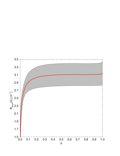
Figure 1: $R_{quark}(\delta)$ as a function of $\delta$.

The ratio $R_{quark}(\delta)$ is divergent in the limit $\delta{\to}1$, which is due to the function $f_{88}(\delta)$. In this limit, the physical quantity to consider would be only the sum of $b{\to}X_{s}\gamma$ and $b{\to}X_{s}$ decay rates, in which this divergence would cancel out.

The divergence at $\delta{\to}1$ is very slow. It manifests itself only by a small kink in Fig. 1 where values of $\delta$ up to 0.999 were included. For $\delta=0.99$, the contribution from $f_{88}(\delta)$ to $R_{quark}(\delta)$ is well below 1%. In order to allow easy comparison with previous experimental and theoretical publications, we choose $\delta^{max}=0.99$ as the first particular value of $\delta$ to consider. This value of $\delta$ will be assumed in discussing the “total” $B{\to}X_{s}\gamma$ decay rate below.

A value of $\delta$ which is closer to what is actually measured is $\delta=z\equiv(m_{c}/m_{b})^{2}$. It corresponds to counting only the photons with energies above the charm production threshold in the $b$-quark rest frame. This is the second value of $\delta$ we will consider below.

We find

$$R_{quark}(\delta^{max}) = (3.12\pm 0.29)\times 10^{-3},$$ (65)

$$R_{quark}(\delta=z) = (2.86\pm 0.24)\times 10^{-3}.$$ (66)

In both cases, the uncertainty is below 10%. The dominant sources of it are $m_{c}/m_{b}$ and $\mu_{b}$. The relative importance of various uncertainties is shown in Table. 1.

	Source
	$\alpha_{s}(M_{Z})$	$m_{t,pole}$	$\mu_{b}$	$m_{c,pole}/m_{b,pole}$	$m_{b,pole}$	$\alpha_{em}$	CKM angles
$\delta=\delta^{max}$	2.5%	1.7%	6.6%	5.2%	0.5%	1.9%	2.1%
$\delta=z$	2.2%	1.7%	3.3%	6.6%	0.6%	1.9%	2.1%

Table I. Uncertainties in $R_{quark}(\delta)$ due to various sources.

Let us note that setting $\delta=z$ introduces an additional spurious inaccuracy due to $m_{c}/m_{b}$ in $R_{quark}$. However, this additional uncertainty is significantly smaller than the original inaccuracy due to $m_{c}/m_{b}$ for $\delta$ uncorrelated with $m_{c}/m_{b}$.

It is quite surprising that the $\mu_{b}$-dependence is weaker for $\delta=z$ than for $\delta=\delta^{max}$. Naively, one would expect larger $\mu_{b}$-dependence for small values of $\delta$, when the first term in eqn. (47) becomes more and more important. Clearly, $\delta=z$ is not small enough for this effect to show up. The weaker $\mu_{b}$-dependence for $\delta=z$ seems to be quite accidental.

6. In the end, we need to pass from the calculated $b$-quark decay rates to the $B$-meson decay rates. Relying on the Heavy Quark Effective Theory (HQET) calculations we write

$${\cal B}(B{\to}X_{s}\gamma)={\cal B}(B{\to}X_{c}e\bar{\nu_{e}})\;\;R_{quark}(\delta^{max})\;\;\left(1-\frac{\delta^{NP}_{sl}}{m_{b}^{2}}+\frac{\delta^{NP}_{rad}}{m_{b}^{2}}\right),$$ (67)

where $\delta^{NP}_{sl}$ and $\delta^{NP}_{rad}$ parametrize nonperturbative corrections to the semileptonic and radiative $B$-meson decay rates, respectively.

Following refs. [3, 30], we express $\delta^{NP}_{sl}$ and $\delta^{NP}_{rad}$ in terms of the HQET parameters $\lambda_{1}$ and $\lambda_{2}$

$$\delta^{NP}_{sl} = \frac{1}{2}\lambda_{1}+\left(\frac{3}{2}-\frac{6(1-z)^{4}}{g(z)}\right)\lambda_{2},$$ (68)

$$\delta^{NP}_{rad} = \frac{1}{2}\lambda_{1}-\frac{9}{2}\lambda_{2},$$ (69)

where $g(z)$ is the same as in eqn. (59). The poorly known parameter $\lambda_{1}$ cancels out in the r.h.s. of eqn. (67) which depends only on the difference $\delta^{NP}_{sl}-\delta^{NP}_{rad}$. The value of $\lambda_{2}$ is known from $B^{*}$–$B$ mass splitting

$$\lambda_{2}=\frac{1}{4}(m_{B^{*}}^{2}-m_{B}^{2})\simeq 0.12\;{\rm GeV}^{2}.$$ (70)

The two nonperturbative corrections in eqn. (67) are both around $4\%$ in magnitude, and they tend to cancel each other. In effect, they sum up to only around $1\%$. Such a small number has to be taken with caution, because the four-quark operators $P_{1}$, …, $P_{6}$ have not been included in the calculation of $\delta^{NP}_{rad}$. Contributions from these operators could potentially give one- or two-percent effects. Nevertheless, it seems reasonable to conclude that the total nonperturbative correction to eqn. (67) is well below 10%, i.e. it is smaller than the inaccuracy of the perturbative calculation of $R_{quark}(\delta^{max})$.

When the above caution is ignored and ${\cal B}(B{\to}X_{c}e\bar{\nu_{e}})=(10.4\pm 0.4)\%$ [23] is used, one obtains the following numerical prediction for $B{\to}X_{s}\gamma$ branching ratio

$${\cal B}(B{\to}X_{s}\gamma)=(3.28\pm 0.33)\times 10^{-4}.$$ (71)

The central value of this prediction is outside the $1\sigma$ experimental error bar in eqn. (2). However, the experimental and theoretical error bars practically touch each other. Therefore, we conclude that the present $B{\to}X_{s}\gamma$ measurement remains in agreement with the Standard Model. This conclusion holds in spite of that the theoretical uncertainty is now more than twice smaller than in the previously available leading order prediction [1].

In the measurement of $B{\to}X_{s}\gamma$ branching fraction, one needs to choose a certain lower bound on photon energies. Instead of talking about the “total” decay rate, it is convenient to count only the photons with energies above the charm production threshold in the $B$-meson rest frame

$$E_{\gamma}>\frac{m_{B}^{2}-m_{D}^{2}}{2m_{B}}\simeq 2.31\;{\rm GeV}.$$ (72)

Most of the photons in $B{\to}X_{s}\gamma$ survive this energy cut, and a huge background from charm production is removed. Let us denote the corresponding branching fraction by ${\cal B}(B{\to}X_{s}\gamma)^{above}$.

If the $b$-quark was infinitely heavy, it would not move inside the $B$-meson. The restriction (72) would then be equivalent to setting $\delta=z$ at the quark level. Since the Fermi motion of the $b$-quark inside the $B$-meson is a ${\cal O}(\bar{\Lambda}/m_{b})$ effect, we can write similarly to eqn. (67)

$${\cal B}(B{\to}X_{s}\gamma)^{above}={\cal B}(B{\to}X_{c}e\bar{\nu})\;\;R_{quark}(\delta=z)\;\;(1+{\cal O}(\bar{\Lambda}/m_{b})).$$ (73)

The ${\cal O}(\bar{\Lambda}/m_{b})$ part of the latter equation can be calculated using specific models for the Fermi motion of the $b$-quark inside the $B$-meson, as it has been done e.g. in ref. [16] (see also ref. [31]). Performing a similar calculation with use of the NLO values of the Wilson coefficients is beyond the scope of the present paper. Such an analysis will be necessary when more statistics allows to reduce experimental errors in measurements of ${\cal B}(B{\to}X_{s}\gamma)^{above}$.

7. To conclude, we have presented practically complete NLO formulae for $b{\to}X_{s}\gamma$ decay in the Standard Model. They include previously published contributions as well as our new results for three-loop anomalous dimensions. Our prediction for $B{\to}X_{s}\gamma$ branching fraction in the Standard Model is $(3.28\pm 0.33)\times 10^{-4}$ which remains in agreement with the CLEO measurement at the $2\sigma$ level. Clearly, an interesting test of the SM will be provided when more precise experimental data are available. More importantly, the $B{\to}X_{s}\gamma$ mode will have more exclusion power for extensions of the SM.

Appendix A.

Here, we give the eight evanescent operators we have used in our anomalous dimension computation. Giving them explicitly is necessary in order to fully specify our renormalization scheme, and thus give meaning to the anomalous dimension matrix presented in eqn. (9).

$$P_{11} = (\bar{s}_{L}\gamma_{\mu_{1}}\gamma_{\mu_{2}}\gamma_{\mu_{3}}T^{a}c_{L})(\bar{c}_{L}\gamma^{\mu_{1}}\gamma^{\mu_{2}}\gamma^{\mu_{3}}T^{a}b_{L})-16P_{1}$$

$$P_{12} = (\bar{s}_{L}\gamma_{\mu_{1}}\gamma_{\mu_{2}}\gamma_{\mu_{3}}c_{L})(\bar{c}_{L}\gamma^{\mu_{1}}\gamma^{\mu_{2}}\gamma^{\mu_{3}}b_{L})-16P_{2}$$

$$P_{15} = (\bar{s}_{L}\gamma_{\mu_{1}}\gamma_{\mu_{2}}\gamma_{\mu_{3}}\gamma_{\mu_{4}}\gamma_{\mu_{5}}b_{L})\sum_{q}(\bar{q}\gamma^{\mu_{1}}\gamma^{\mu_{2}}\gamma^{\mu_{3}}\gamma^{\mu_{4}}\gamma^{\mu_{5}}q)-20P_{5}+64P_{3}$$

$$P_{16} = (\bar{s}_{L}\gamma_{\mu_{1}}\gamma_{\mu_{2}}\gamma_{\mu_{3}}\gamma_{\mu_{4}}\gamma_{\mu_{5}}T^{a}b_{L})\sum_{q}(\bar{q}\gamma^{\mu_{1}}\gamma^{\mu_{2}}\gamma^{\mu_{3}}\gamma^{\mu_{4}}\gamma^{\mu_{5}}T^{a}q)-20P_{6}+64P_{4}$$

$$P_{21} = (\bar{s}_{L}\gamma_{\mu_{1}}\gamma_{\mu_{2}}\gamma_{\mu_{3}}\gamma_{\mu_{4}}\gamma_{\mu_{5}}T^{a}c_{L})(\bar{c}_{L}\gamma^{\mu_{1}}\gamma^{\mu_{2}}\gamma^{\mu_{3}}\gamma^{\mu_{4}}\gamma^{\mu_{5}}T^{a}b_{L})-20P_{11}-256P_{1}$$ (74)

$$P_{22} = (\bar{s}_{L}\gamma_{\mu_{1}}\gamma_{\mu_{2}}\gamma_{\mu_{3}}\gamma_{\mu_{4}}\gamma_{\mu_{5}}Tc_{L})(\bar{c}_{L}\gamma^{\mu_{1}}\gamma^{\mu_{2}}\gamma^{\mu_{3}}\gamma^{\mu_{4}}\gamma^{\mu_{5}}b_{L})-20P_{12}-256P_{2}$$

$$P_{25} = (\bar{s}_{L}\gamma_{\mu_{1}}\gamma_{\mu_{2}}\gamma_{\mu_{3}}\gamma_{\mu_{4}}\gamma_{\mu_{5}}\gamma_{\mu_{6}}\gamma_{\mu_{7}}b_{L})\sum_{q}(\bar{q}\gamma^{\mu_{1}}\gamma^{\mu_{2}}\gamma^{\mu_{3}}\gamma^{\mu_{4}}\gamma^{\mu_{5}}\gamma^{\mu_{6}}\gamma^{\mu_{7}}q)-336P_{5}+1280P_{3}$$

$$P_{26} = (\bar{s}_{L}\gamma_{\mu_{1}}\gamma_{\mu_{2}}\gamma_{\mu_{3}}\gamma_{\mu_{4}}\gamma_{\mu_{5}}\gamma_{\mu_{6}}\gamma_{\mu_{7}}T^{a}b_{L})\sum_{q}(\bar{q}\gamma^{\mu_{1}}\gamma^{\mu_{2}}\gamma^{\mu_{3}}\gamma^{\mu_{4}}\gamma^{\mu_{5}}\gamma^{\mu_{6}}\gamma^{\mu_{7}}T^{a}q)-336P_{6}+1280P_{4}.$$

Appendix B.

Here, we express the functions $f_{ij}(\delta)$ present in eqn. (47) in terms of the quantities $M_{kl}(t,u)$ given in eqn. (27) of ref. [17]. For each $(ij)\neq(77)$ and $i\leq j$, $f_{ij}(\delta)$ is given by

$$f_{ij}(\delta)=\frac{2}{3}(2-\delta_{ij})\sum_{\stackrel{{\scriptstyle k,l=1}}{{k\leq l}}}^{8}W_{ik}\left[\int_{1-\delta}^{1}du\int_{1-u}^{1}dt\;M_{kl}(t,u)\right]W_{jl},$$ (75)

where

$$\hat{W}=\left[\begin{array}[]{cccccccc}\frac{1}{2}&-\frac{1}{6}&0&0&0&0&0&0\\ 0&1&0&0&0&0&0&0\\ 0&0&1&0&1&0&0&0\\ 0&0&-\frac{1}{6}&\frac{1}{2}&-\frac{1}{6}&\frac{1}{2}&0&0\\ 0&0&16&0&4&0&0&0\\ 0&0&-\frac{8}{3}&8&-\frac{2}{3}&2&0&0\\ 0&0&0&0&0&0&1&0\\ 0&0&0&0&0&0&0&1\end{array}\right]$$ (76)

In four space-time dimensions, the matrix $\hat{W}$ transforms our operator basis (4) into the one used in ref. [17]

$$P_{i}\;\;\stackrel{{\scriptstyle D=4}}{{===}}\;\;\sum_{k=1}^{8}W_{ik}\hat{O}_{k}.$$ (77)

References

[1] A. J. Buras, M. Misiak, M. Münz, and S. Pokorski,
Nucl. Phys. B424 (1994) 374.
[2] J. Hewett, “Top ten models constrained by ”,
published in proceedings “Spin structure in
high energy processes”, p. 463, Stanford, 1993.
[3] A.F. Falk, M. Luke and M. Savage, Phys. Rev. D49 (1994) 3367.
[4] M.S. Alam et al., Phys. Rev. Lett. 74 (1995) 2885.
[5] A. Ali and C. Greub Phys. Lett. B293 (1992) 226.
[6] B. Grinstein, R. Springer and M.B. Wise, Nucl. Phys. B339 (1990) 269.
[7] R. Grigjanis, P.J. O’Donnell, M. Sutherland and H. Navelet,
Phys. Lett. B213 (1999) 355, Phys. Lett. B286 (1992) 413(E).
[8] M. Ciuchini, E. Franco, G. Martinelli, L. Reina and
L. Silvestrini, Phys. Lett. B316 (1993) 127;
M. Ciuchini, E. Franco, L. Reina and
L. Silvestrini, Nucl. Phys. B421 (1994) 41.
[9] C. Greub, T. Hurth and D. Wyler,
Phys. Lett. B380 (1996) 385, Phys. Rev. D54 (1996) 3350.
[10] A. J. Buras, M. Jamin, M. E. Lautenbacher and P .H. Weisz,
Nucl. Phys. B370 (1992) 69, Nucl. Phys. B375 (1992) 501 (addendum).
[11] M. Ciuchini, E. Franco, G. Martinelli and L. Reina,
Nucl. Phys. B415 (1994) 403.
[12] M. Misiak and M. Münz, Phys. Lett. B344 (1995) 308.
[13] K. Adel and Y.P. Yao, Phys. Rev. D49 (1994) 4945.
[14] P. Cho, B. Grinstein, Nucl. Phys. B365 (1991) 279.
[15] A. Ali and C. Greub,
Z. Phys. C49 (1991) 431, Phys. Lett. B259 (1991) 182.
[16] A. Ali and C. Greub, Phys. Lett. B361 (1995) 146
(equation numbers refer to the preprint version hep-ph/9506374).
[19] M. J. Dugan and B. Grinstein, Phys. Lett. B256 (1991) 239.
[20] S. Herrlich and U. Nierste, Nucl. Phys. B455 (1995) 39.
[21] K. Chetyrkin, M. Misiak and M. Münz, in preparation.
[22] T. Inami and C. S. Lim, Prog. Theor. Phys. 65 (1981) 297,
65 (1981) 1772E.
[23] Particle Data Group, Phys. Rev. D54 (1996) 1.
[24] M. Schmelling, plenary talk given at the ICHEP96 conference,
Warsaw, July 1996.
[25] P. Tipton, plenary talk given at the ICHEP96 conference,
Warsaw, July 1996.
[26] A. Kapustin, Z. Ligeti and H. D. Politzer, Phys. Lett. B357 (1995) 653.
[27] N. Cabibbo and L. Maiani, Phys. Lett. B79 (1978) 109.
[28] Y. Nir, Phys. Lett. B221 (1989) 184.
[29] A.J. Buras, plenary talk given at the ICHEP96 conference,
Warsaw, July 1996
(hep-ph/9610461).
[30] M. Neubert, Proc. of the 17th Symposium on Lepton-Photon
Interactions, Beijing, 1995, ed. by Z. Zhi-Peng and C. He-Sheng, World
Scientific 1996 (and references therein).