Tau Lepton Physics: Theory Overview

Abstract

The pure leptonic or semileptonic character of $\tau$ decays makes them a good laboratory to test the structure of the weak currents and the universality of their couplings to the gauge bosons. The hadronic $\tau$ decay modes constitute an ideal tool for studying low–energy effects of the strong interactions in very clean conditions; a well–known example is the precise determination of the QCD coupling from $\tau$–decay data. New physics phenomena, such as a non-zero $m_{\nu_{\tau}}$ or violations of (flavour / CP) conservation laws can also be searched for with $\tau$ decays.

FTUV/96-87
IFIC/96-96

1 INTRODUCTION

The $\tau$ lepton is a member of the third generation which decays into particles belonging to the first and second ones. Thus, $\tau$ physics could provide some clues to the puzzle of the recurring families of leptons and quarks. In fact, one naïvely expects the heavier fermions to be more sensitive to whatever dynamics is responsible for the fermion–mass generation.

The pure leptonic or semileptonic character of $\tau$ decays provides a clean laboratory to test the structure of the weak currents and the universality of their couplings to the gauge bosons. Moreover, the $\tau$ is the only known lepton massive enough to decay into hadrons; its semileptonic decays are then an ideal tool for studying strong interaction effects in very clean conditions.

The last few years have witnessed a substantial change on our knowledge of the $\tau$ properties [1]. The large (and clean) data samples collected by the most recent experiments have improved considerably the statistical accuracy and, moreover, have brought a new level of systematic understanding. All experimental results obtained so far confirm the Standard Model (SM) scenario, in which the $\tau$ is a sequential lepton with its own quantum number and associated neutrino.

With the increased sensitivities achieved recently, interesting limits on possible new physics contributions to the $\tau$ decay amplitudes start to emerge. The present tests on lepton universality will be reviewed in section 2, both for the charged and neutral current sectors. The Lorentz structure of the leptonic charged currents will be discussed in section 3. The quality of the hadronic $\tau$–decay data allows to study important properties of low–energy QCD, involving both perturbative and non-perturbative aspects; this will be addressed in section 4. Section 5 contains a brief overview of several searches for new physics phenomena, using $\tau$ decays. A few summarizing comments will be finally given in section 6.

2 UNIVERSALITY

2.1 Charged Currents

The leptonic decays $\tau^{-}\to e^{-}\bar{\nu}_{e}\nu_{\tau},\mu^{-}\bar{\nu}_{\mu}\nu_{\tau}$ are theoretically understood at the level of the electroweak radiative corrections [2]. Within the SM,

$$\Gamma(\tau^{-}\rightarrow\nu_{\tau}l^{-}\bar{\nu}_{l})\,=\,{G_{F}^{2}m_{\tau}^{5}\over 192\pi^{3}}\,f(m_{l}^{2}/m_{\tau}^{2})\,r_{EW},$$ (1)

where $f(x)=1-8x+8x^{3}-x^{4}-12x^{2}\log{x}$. The factor $r_{EW}=0.9960$ takes into account radiative corrections not included in the Fermi coupling constant $G_{F}$, and the non-local structure of the $W$ propagator [2].

Table 1: Average values [4, 5, 6, 7] of some basic $\tau$ parameters. $h^{-}$ stands for either $\pi^{-}$ or $K^{-}$.

$m_{\tau}$	$(1777.00^{+0.30}_{-0.27})$ MeV
$\tau_{\tau}$	$(290.21\pm 1.15)$ fs
$B_{e}$	$(17.786\pm 0.072)\%$
$B_{\mu}$	$(17.317\pm 0.078)\%$
Br($\tau^{-}\to\nu_{\tau}\pi^{-}$)	$(11.01\pm 0.11)\%$
Br($\tau^{-}\to\nu_{\tau}K^{-}$)	$(0.692\pm 0.028)\%$
Br($\tau^{-}\to\nu_{\tau}h^{-}$)	$(11.70\pm 0.11)\%$

Figure 1: Relation between $B_{e}$ and $\tau_{\tau}$. The dotted band corresponds to the prediction in Eq. (2).

Using the value of $G_{F}$ measured in $\mu$ decay, Eq. (1) provides a relation [3] between the $\tau$ lifetime and the leptonic branching ratios $B_{l}\equiv B(\tau^{-}\to\nu_{\tau}l^{-}\bar{\nu}_{l})$:

$$B_{e} = {B_{\mu}\over 0.972564\pm 0.000010}$$ (2)

$$= {\tau_{\tau}\over(1.6321\pm 0.0014)\times 10^{-12}\,{\rm s}}\,.$$

The errors reflect the present uncertainty of $0.3$ MeV in the value of $m_{\tau}$.

The relevant experimental measurements are given in Table 1. The predicted $B_{\mu}/B_{e}$ ratio is in perfect agreement with the measured value $B_{\mu}/B_{e}=0.974\pm 0.006$. As shown in Fig. 1, the relation between $B_{e}$ and $\tau_{\tau}$ is also well satisfied by the present data. Notice, that this relation is very sensitive to the value of the $\tau$ mass [$\Gamma_{\tau\to l}\propto m_{\tau}^{5}$]. The most recent measurements of $\tau_{\tau}$, $B_{e}$ and $m_{\tau}$ have consistently moved the world averages in the correct direction, eliminating the previous ($\sim 2\sigma$) disagreement. The experimental precision (0.4%) is already approaching the level where a possible non-zero $\nu_{\tau}$ mass could become relevant; the present bound [8] $m_{\nu_{\tau}}<24$ MeV (95% CL) only guarantees that such effect is below 0.14%.

The decay modes $\tau^{-}\to\nu_{\tau}P^{-}$ [$P=\pi,K$] can also be accurately predicted through the ratios $R_{\tau/P}\equiv\Gamma(\tau^{-}\to\nu_{\tau}P^{-})/\Gamma(P^{-}\to\mu^{-}\bar{\nu}_{\mu})$, where the dependence on the hadronic matrix elements (the so–called decay constants $f_{P}$) factors out:

$$R_{\tau/P}={m_{\tau}^{3}\over 2m_{P}m_{\mu}^{2}}{(1-m_{P}^{2}/m_{\tau}^{2})^{2}\over(1-m_{\mu}^{2}/m_{P}^{2})^{2}}\left(1+\delta R_{\tau/P}\right).$$ (3)

Owing to the different energy scales involved, the radiative corrections to the $\tau^{-}\to\nu_{\tau}P^{-}$ amplitudes are however not the same than the corresponding effects in $P^{-}\to\mu^{-}\bar{\nu}_{\mu}$. The relative correction has been estimated [10, 11] to be:

$$\delta R_{\tau/\pi} = (0.16\pm 0.14)\%\ ,$$

$$\delta R_{\tau/K} = (0.90\pm 0.22)\%\ .$$ (4)

All these measurements can be used to test the universality of the $W$ couplings to the leptonic charged currents. The $B_{\mu}/B_{e}$ ratio constraints $|g_{\mu}/g_{e}|$, while $B_{e}/\tau_{\tau}$ and $R_{\tau/P}$ provide information on $|g_{\tau}/g_{\mu}|$. The present results are shown in Tables 3 and 3, together with the values obtained from the ratio [12] $R_{\pi\to e/\mu}\equiv\Gamma(\pi^{-}\to e^{-}\bar{\nu}_{e})/\Gamma(\pi^{-}\to\mu^{-}\bar{\nu}_{\mu})$, and from the comparison of the $\sigma\cdot B$ partial production cross-sections for the various $W^{-}\to l^{-}\bar{\nu}_{l}$ decay modes at the $p$-$\bar{p}$ colliders [13].

Table 2: Present constraints on $|g_{\mu}/g_{e}|$.

	$|g_{\mu}/g_{e}|$
$B_{\mu}/B_{e}$	$1.0005\pm 0.0030$
$R_{\pi\to e/\mu}$	$1.0017\pm 0.0015$
$\sigma\cdot B_{W\to\mu/e}$	$1.01\pm 0.04$

Table 3: Present constraints on $|g_{\tau}/g_{\mu}|$.

	$|g_{\tau}/g_{\mu}|$
$B_{e}\tau_{\mu}/\tau_{\tau}$	$1.0001\pm 0.0029$
$R_{\tau/\pi}$	$1.005\pm 0.005$
$R_{\tau/K}$	$0.984\pm 0.020$
$R_{\tau/h}$	$1.004\pm 0.005$
$\sigma\cdot B_{W\to\tau/\mu}$	$0.99\pm 0.05$

The present data verifies the universality of the leptonic charged–current couplings to the 0.15% ($e/\mu$) and 0.30% ($\tau/\mu$) level. The precision of the most recent $\tau$–decay measurements is becoming competitive with the more accurate $\pi$–decay determination. It is important to realize the complementarity of the different universality tests. The pure leptonic decay modes probe the charged–current couplings of a transverse $W$. In contrast, the decays $\pi/K\to l\bar{\nu}$ and $\tau\to\nu_{\tau}\pi/K$ are only sensitive to the spin–0 piece of the charged current; thus, they could unveil the presence of possible scalar–exchange contributions with Yukawa–like couplings proportional to some power of the charged–lepton mass. One can easily imagine new physics scenarios which would modify differently the two types of leptonic couplings [14]. For instance, in the usual two Higgs doublet model, charged–scalar exchange generates a correction to the ratio $B_{\mu}/B_{e}$, but $R_{\pi\to e/\mu}$ remains unaffected. Similarly, lepton mixing between the $\nu_{\tau}$ and an hypothetical heavy neutrino would not modify the ratios $B_{\mu}/B_{e}$ and $R_{\pi\to e/\mu}$, but would certainly correct the relation between $B_{l}$ and the $\tau$ lifetime.

2.2 Neutral Currents

In the SM, all leptons with equal electric charge have identical couplings to the $Z$ boson: $v_{l}=T_{3}^{l}(1-4|Q_{l}|\sin^{2}{\theta_{W}})$, $a_{l}=T_{3}^{l}$. This has been tested at LEP and SLC [15, 16], where the effective vector and axial–vector couplings of the three charged leptons have been determined, by measuring the total $e^{+}e^{-}\to Z\to l^{+}l^{-}$ cross–section, the forward–backward asymmetry, the (final) polarization asymmetry, the forward–backward (final) polarization asymmetry, and (at SLC) the left–right asymmetry between the cross–sections for initial left– and right–handed electrons:

$$\sigma^{0,l}={12\pi\over M_{Z}^{2}}\,{\Gamma_{e}\Gamma_{l}\over\Gamma_{Z}^{2}}\,,\qquad\;{\cal A}_{\mbox{\rm\scriptsize FB}}^{0,l}={3\over 4}{\cal P}_{e}{\cal P}_{l}\,,$$

$${\cal A}_{\mbox{\rm\scriptsize Pol}}^{0,l}={\cal P}_{l}\,,\qquad\qquad\quad{\cal A}_{\mbox{\rm\scriptsize FB,Pol}}^{0,l}={3\over 4}{\cal P}_{e}\,,$$ (5)

$${\cal A}_{\mbox{\rm\scriptsize LR}}^{0}=-{\cal P}_{e}\,,$$

where

$${\cal P}_{l}\,\equiv\,{-2v_{l}a_{l}\over v_{l}^{2}+a_{l}^{2}}$$ (6)

is the average longitudinal polarization of the lepton $l^{-}$.

The $Z$ partial decay width to the $l^{+}l^{-}$ final state,

$$\Gamma_{l}={G_{F}M_{Z}^{3}\over 6\pi\sqrt{2}}\,(v_{l}^{2}+a_{l}^{2})\,\left(1+{3\alpha\over 4\pi}\right),$$ (7)

determines the sum $(v_{l}^{2}+a_{l}^{2})$, while the ratio $v_{l}/a_{l}$ is derived from the asymmetries. The signs of $v_{l}$ and $a_{l}$ are fixed by requiring $a_{e}<0$.

The measurement of the final polarization asymmetries can (only) be done for $l=\tau$, because the spin polarization of the $\tau$’s is reflected in the distorted distribution of their decay products. Therefore, ${\cal P}_{\tau}$ and ${\cal P}_{e}$ can be determined from a measurement of the spectrum of the final charged particles in the decay of one $\tau$, or by studying the correlated distributions between the final products of both $\tau^{\prime}s$ [17].

Table 4: Measured values [16] of $\Gamma_{l}\equiv\Gamma(Z\to l^{+}l^{-})$ and the leptonic forward–backward asymmetries. The last column shows the combined result (for a massless lepton) assuming lepton universality.

	$e$	$\mu$	$\tau$	$l$
$\Gamma_{l}$   (MeV)	$83.96\pm 0.15$	$83.79\pm 0.22$	$83.72\pm 0.26$	$83.91\pm 0.11$
${\cal A}_{\mbox{\rm\scriptsize FB}}^{0,l}$   (%)	$1.60\pm 0.24$	$1.62\pm 0.13$	$2.01\pm 0.18$	$1.74\pm 0.10$

Table 5: Measured values [16] of the different polarization asymmetries.

${\cal A}_{\mbox{\rm\scriptsize Pol}}^{0,\tau}={\cal P}_{\tau}$	${4\over 3}{\cal A}^{0,\tau}_{\mbox{\rm\scriptsize FB,Pol}}={\cal P}_{e}$	$-{\cal A}_{\mbox{\rm\scriptsize LR}}^{0}={\cal P}_{e}$	$-\{{4\over 3}{\cal A}_{\mbox{\rm\scriptsize FB}}^{0,l}\}^{1/2}=P_{l}$
$-0.1401\pm 0.0067$	$-0.1382\pm 0.0076$	$-0.1542\pm 0.0037$	$-0.1523\pm 0.0044$

Tables 5 and 5 show the present experimental results for the leptonic $Z$–decay widths and asymmetries. The data are in excellent agreement with the SM predictions and confirm the universality of the leptonic neutral couplings. There is however a small ($\sim 2\sigma$) discrepancy between the ${\cal P}_{e}$ values obtained [16] from ${\cal A}^{0,\tau}_{\mbox{\rm\scriptsize FB,Pol}}$ and ${\cal A}_{\mbox{\rm\scriptsize LR}}^{0}$. Assuming lepton universality, the combined result from all leptonic asymmetries gives

$${\cal P}_{l}=-0.1500\pm 0.0025\ .$$ (8)

The measurement of ${\cal A}_{\mbox{\rm\scriptsize Pol}}^{0,\tau}$ and ${\cal A}^{0,\tau}_{\mbox{\rm\scriptsize FB,Pol}}$ assumes that the $\tau$ decay proceeds through the SM charged–current interaction. A more general analysis should take into account the fact that the $\tau$–decay width depends on the product $\xi{\cal P}_{\tau}$ (see section 3), where $\xi$ is the corresponding Michel parameter in leptonic decays, or the equivalent quantity $\xi_{h}$ ($=h_{\nu_{\tau}}$) in the semileptonic modes. A separate measurement of $\xi$ and ${\cal P}_{\tau}$ has been performed by ALEPH [18] (${\cal P}_{\tau}=-0.139\pm 0.040$) and L3 [19] (${\cal P}_{\tau}=-0.154\pm 0.022$), using the correlated distribution of the $\tau^{+}\tau^{-}$ decays.

The combined analysis of all leptonic observables from LEP and SLD (${\cal A}_{\mbox{\rm\scriptsize LR}}^{0}$) results in the effective vector and axial–vector couplings given in Table 6 [16]. The corresponding 68% probability contours in the $a_{l}$–$v_{l}$ plane are shown in Fig. 2. The measured ratios of the $e$, $\mu$ and $\tau$ couplings provide a test of charged–lepton universality in the neutral–current sector.

The neutrino coupling can be determined from the invisible $Z$–decay width, by assuming three identical neutrino generations with left–handed couplings (i.e., $v_{\nu}=a_{\nu}$), and fixing the sign from neutrino scattering data [20]. The resulting experimental value [16], given in Table 6, is in perfect agreement with the SM. Alternatively, one can use the SM prediction for $\Gamma_{\mbox{\rm\scriptsize inv}}/\Gamma_{l}$ to get a determination of the number of (light) neutrino flavours [16]: $N_{\nu}=2.989\pm 0.012$. The universality of the neutrino couplings has been tested with $\nu_{\mu}e$ scattering data, which fixes [21] the $\nu_{\mu}$ coupling to the $Z$:  $v_{\nu_{\mu}}=a_{\nu_{\mu}}=0.502\pm 0.017$.

The measured leptonic asymmetries can be used to obtain the effective electroweak mixing angle in the charged–lepton sector: [16]

$$\sin^{2}{\theta^{\mbox{\rm\scriptsize lept}}_{\mbox{\rm\scriptsize eff}}}\equiv{1\over 4}\left(1-{v_{l}\over a_{l}}\right)=0.23114\pm 0.00031\,.$$ (9)

Including also the hadronic asymmetries, one gets [16] $\sin^{2}{\theta^{\mbox{\rm\scriptsize lept}}_{\mbox{\rm\scriptsize eff}}}=0.23165\pm 0.00024$ with a $\chi^{2}/\mbox{\rm d.o.f.}=12.8/6$.

Table 6: Effective vector and axial–vector lepton couplings derived from LEP and SLD data [16].

$v_{e}$	$-0.03828\pm 0.00079$
$v_{\mu}$	$-0.0358\pm 0.0030$
$v_{\tau}$	$-0.0367\pm 0.0016$
$a_{e}$	$-0.50119\pm 0.00045$
$a_{\mu}$	$-0.50086\pm 0.00068$
$a_{\tau}$	$-0.50117\pm 0.00079$
$v_{\mu}/v_{e}$	$\phantom{-}0.935\pm 0.085$
$v_{\tau}/v_{e}$	$\phantom{-}0.959\pm 0.046$
$a_{\mu}/a_{e}$	$\phantom{-}0.9993\pm 0.0017$
$a_{\tau}/a_{e}$	$\phantom{-}1.0000\pm 0.0019$
With Lepton Universality
$v_{l}$	$-0.03776\pm 0.00062$
$a_{l}$	$-0.50108\pm 0.00034$
$a_{\nu}=v_{\nu}$	$+0.5009\pm 0.0010$

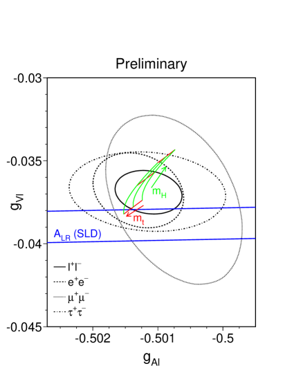
Figure 2: 68% probability contours in the $a_{l}$-$v_{l}$ plane from LEP measurements [16]. The solid contour assumes lepton universality. Also shown is the $1\sigma$ band resulting from the ${\cal A}_{\mbox{\rm\scriptsize LR}}^{0}$ measurement at SLD. The grid corresponds to the SM prediction.

3 LORENTZ STRUCTURE

Let us consider the decay $l^{-}\to\nu_{l}l^{\prime-}\bar{\nu}_{l^{\prime}}$, where the lepton pair ($l$, $l^{\prime}$) may be ($\mu$, $e$), ($\tau$, $e$), or ($\tau$, $\mu$). The most general, local, derivative–free, lepton–number conserving, four–lepton interaction Hamiltonian, consistent with locality and Lorentz invariance [22, 23, 24, 25, 26, 27],

$${\cal H}=4\frac{G_{l^{\prime}l}}{\sqrt{2}}\sum_{n,\epsilon,\omega}g^{n}_{\epsilon\omega}\left[\overline{l^{\prime}_{\epsilon}}\Gamma^{n}{(\nu_{l^{\prime}})}_{\sigma}\right]\,\left[\overline{({\nu_{l}})_{\lambda}}\Gamma_{n}l_{\omega}\right]\ ,$$ (10)

contains ten complex coupling constants or, since a common phase is arbitrary, nineteen independent real parameters which could be different for each leptonic decay. The subindices $\epsilon,\omega,\sigma,\lambda$ label the chiralities (left–handed, right–handed) of the corresponding fermions, and $n$ the type of interaction: scalar ($I$), vector ($\gamma^{\mu}$), tensor ($\sigma^{\mu\nu}/\sqrt{2}$). For given $n,\epsilon,\omega$, the neutrino chiralities $\sigma$ and $\lambda$ are uniquely determined.

Taking out a common factor $G_{l^{\prime}l}$, which is determined by the total decay rate, the coupling constants $g^{n}_{\epsilon\omega}$ are normalized to [25]

$$1 \!\!\!= \!\!\!{1\over 4}\,\left(|g^{S}_{RR}|^{2}+|g^{S}_{RL}|^{2}+|g^{S}_{LR}|^{2}+|g^{S}_{LL}|^{2}\right)$$ (11)

$$\!\!\!\mbox{}+\left(|g^{V}_{RR}|^{2}+|g^{V}_{RL}|^{2}+|g^{V}_{LR}|^{2}+|g^{V}_{LL}|^{2}\right)$$

$$\!\!\!\mbox{}+3\,\left(|g^{T}_{RL}|^{2}+|g^{T}_{LR}|^{2}\right)\,.$$

In the SM, $g^{V}_{LL}=1$ and all other $g^{n}_{\epsilon\omega}=0$.

For an initial lepton polarization ${\cal P}_{l}$, the final charged–lepton distribution in the decaying–lepton rest frame is usually parameterized [23] in the form

$${d^{2}\Gamma\over dx\,d\cos\theta}={m_{l}\omega^{4}\over 2\pi^{3}}G_{l^{\prime}l}^{2}\sqrt{x^{2}-x_{0}^{2}}$$ (12)

$$\times\left\{F(x)-{\xi\over 3}\,{\cal P}_{l}\,\sqrt{x^{2}-x_{0}^{2}}\,\cos{\theta}\,A(x)\right\},$$

where $\theta$ is the angle between the $l^{-}$ spin and the final charged–lepton momentum, $\,\omega\equiv(m_{l}^{2}+m_{l^{\prime}}^{2})/2m_{l}\,$ is the maximum $l^{\prime-}$ energy for massless neutrinos, $x\equiv E_{l^{\prime-}}/\omega$ is the reduced energy, $x_{0}\equiv m_{l^{\prime}}/\omega$ and

$$F(x) \!\!\!= \!\!\!x(1-x)+{2\over 9}\rho\left(4x^{2}-3x-x_{0}^{2}\right)$$ (13)

$$\!\!\!\!\mbox{}+\eta\,x_{0}(1-x)\,,$$

$$A(x) \!\!\!= \!\!\!1-x+{2\over 3}\delta\left(4x-4+\sqrt{1-x_{0}^{2}}\right)\,.$$

For unpolarized $l^{\prime}s$, the distribution is characterized by the so-called Michel [22] parameter $\rho$ and the low–energy parameter $\eta$. Two more parameters, $\xi$ and $\delta$, can be determined when the initial lepton polarization is known. If the polarization of the final charged lepton is also measured, 5 additional independent parameters [4] ($\xi^{\prime}$, $\xi^{\prime\prime}$, $\eta^{\prime\prime}$, $\alpha^{\prime}$, $\beta^{\prime}$) appear.

For massless neutrinos, the total decay rate is still given by Eq. (1), but changing $G_{F}$ to [27]

$$\widehat{G}_{l^{\prime}l}\equiv G_{l^{\prime}l}\,\sqrt{1+4\,\eta\,{m_{l^{\prime}}\over m_{l}}\,{g\!\left(m_{l^{\prime}}^{2}/m_{l}^{2}\right)\over f\!\left(m_{l^{\prime}}^{2}/m_{l}^{2}\right)}}\,,$$ (14)

where $g(z)=1+9z-9z^{2}-z^{3}+6z(1+z)\ln{z}$. Thus, $\widehat{G}_{e\mu}$ corresponds to the Fermi coupling $G_{F}$, measured in $\mu$ decay. The $B_{\mu}/B_{e}$ and $B_{e}\tau_{\mu}/\tau_{\tau}$ universality tests, discussed in the previous section, actually prove the ratios $|\widehat{G}_{\mu\tau}/\widehat{G}_{e\tau}|$ and $|\widehat{G}_{e\tau}/\widehat{G}_{e\mu}|$, respectively. An important point, emphatically stressed by Fetscher and Gerber [26], concerns the extraction of $G_{e\mu}$, whose uncertainty is dominated by the uncertainty in $\eta_{\mu\to e}$.

In terms of the $g_{\epsilon\omega}^{n}$ couplings, the shape parameters in Eqs. (12) and (13) are:

$$\rho={3\over 4}(\beta^{+}+\beta^{-})+(\gamma^{+}+\gamma^{-})\,,$$

$$\xi=3(\alpha^{-}-\alpha^{+})+(\beta^{-}-\beta^{+})+{7\over 3}(\gamma^{+}-\gamma^{-})\,,$$

$$\xi\delta={3\over 4}(\beta^{-}-\beta^{+})+(\gamma^{+}-\gamma^{-})\,,$$ (15)

$$\eta=\frac{1}{2}\mbox{\rm Re}\left[g^{V}_{LL}g^{S\ast}_{RR}+g^{V}_{RR}g^{S\ast}_{LL}+g^{V}_{LR}\left(g^{S\ast}_{RL}+6g^{T\ast}_{RL}\right)\right.$$

$$\left.\qquad\mbox{}+g^{V}_{RL}\left(g^{S\ast}_{LR}+6g^{T\ast}_{LR}\right)\right],$$

where [28]

$$\alpha^{+}\equiv{|g^{V}_{RL}|}^{2}+{1\over 16}{|g^{S}_{RL}+6g^{T}_{RL}|}^{2}\,,$$

$$\beta^{+}\equiv{|g^{V}_{RR}|}^{2}+{1\over 4}{|g^{S}_{RR}|}^{2}\,,$$ (16)

$$\gamma^{+}\equiv{3\over 16}{|g^{S}_{RL}-2g^{T}_{RL}|}^{2}\,,$$

are positive–definite combinations of decay constants, corresponding to a final right–handed lepton, while $\alpha^{-}$, $\beta^{-}$, $\gamma^{-}$ denote the corresponding combinations with opposite chiralities ($R\leftrightarrow L$). In the SM, $\rho=\delta=3/4$, $\eta=\eta^{\prime\prime}=\alpha^{\prime}=\beta^{\prime}=0$ and $\xi=\xi^{\prime}=\xi^{\prime\prime}=1$.

The normalization constraint (11) is equivalent to $\alpha^{+}+\alpha^{-}+\beta^{+}+\beta^{-}+\gamma^{+}+\gamma^{-}=1$. It is convenient to introduce [25] the probabilities $Q_{\epsilon\omega}$ for the decay of an $\omega$–handed $l^{-}$ into an $\epsilon$–handed daughter lepton,

$$Q_{LL}=\beta^{-}={1\over 4}|g^{S}_{LL}|^{2}\!+|g^{V}_{LL}|^{2}\,,$$

$$Q_{RR}=\beta^{+}={1\over 4}|g^{S}_{RR}|^{2}\!+\!|g^{V}_{RR}|^{2}\,,$$ (17)

$$Q_{LR}=\alpha^{-}+\gamma^{-}={1\over 4}|g^{S}_{LR}|^{2}\!+\!|g^{V}_{LR}|^{2}\!+\!3|g^{T}_{LR}|^{2}\,,$$

$$Q_{RL}=\alpha^{+}+\gamma^{+}={1\over 4}|g^{S}_{RL}|^{2}\!+\!|g^{V}_{RL}|^{2}\!+\!3|g^{T}_{RL}|^{2}\,.$$

Upper bounds on any of these (positive–semidefinite) probabilities translate into corresponding limits for all couplings with the given chiralities.

For $\mu$ decay, where precise measurements of the polarizations of both $\mu$ and $e$ have been performed, there exist [25] upper bounds on $Q_{RR}$, $Q_{LR}$ and $Q_{RL}$, and a lower bound on $Q_{LL}$. They imply corresponding upper bounds on the 8 couplings $|g^{n}_{RR}|$, $|g^{n}_{LR}|$ and $|g^{n}_{RL}|$. The measurements of the $\mu^{-}$ and the $e^{-}$ do not allow to determine $|g^{S}_{LL}|$ and $|g^{V}_{LL}|$ separately [25, 29]. Nevertheless, since the helicity of the $\nu_{\mu}$ in pion decay is experimentally known [30] to be $-1$, a lower limit on $|g^{V}_{LL}|$ is obtained [25] from the inverse muon decay $\nu_{\mu}e^{-}\to\mu^{-}\nu_{e}$. The present (90% CL) bounds [4] on the $\mu$–decay couplings are shown in Fig. 3. These limits show nicely that the bulk of the $\mu$–decay transition amplitude is indeed of the predicted V$-$A type.

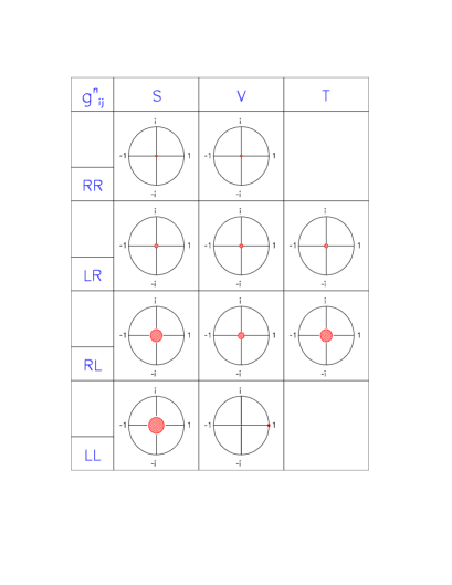
Figure 3: 90% CL experimental limits [4] for the normalized $\mu$–decay couplings $g^{\prime n}_{\epsilon\omega}\equiv g^{n}_{\epsilon\omega}/N^{n}$, where $N^{n}\equiv\mbox{\rm max}(|g^{n}_{\epsilon\omega}|)=2$, 1, $1/\sqrt{3}$ for $n=$ S, V, T. (Taken from Ref. [41]).

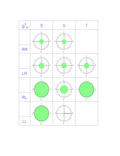
Figure 4: 90% CL experimental limits for the normalized $\tau$–decay couplings $g^{\prime n}_{\epsilon\omega}\equiv g^{n}_{\epsilon\omega}/N^{n}$, assuming $e/\mu$ universality.

The experimental analysis of the $\tau$–decay parameters is necessarily different from the one applied to the muon, because of the much shorter $\tau$ lifetime. The measurement of the $\tau$ polarization and the parameters $\xi$ and $\delta$ is still possible due to the fact that the spins of the $\tau^{+}\tau^{-}$ pair produced in $e^{+}e^{-}$ annihilation are strongly correlated [17, 31, 32, 33, 34, 35, 36]. Another possibility is to use the beam polarization, as done by SLD [37]. However, the polarization of the charged lepton emitted in the $\tau$ decay has never been measured. In principle, this could be done for the decay $\tau^{-}\to\mu^{-}\bar{\nu}_{\mu}\nu_{\tau}$ by stopping the muons and detecting their decay products [34, 38]. The measurement of the inverse decay $\nu_{\tau}l^{-}\to\tau^{-}\nu_{l}$ looks far out of reach.

The present experimental status [5] on the $\tau$–decay Michel parameters is shown in Table 8. For comparison, the values measured in $\mu$ decay [4] are also given. The improved accuracy of the most recent experimental analyses has brought an enhanced sensitivity to the different shape parameters, allowing the first measurements of $\eta_{\tau\to\mu}$, $\xi_{\tau\to e}$, $\xi_{\tau\to\mu}$, $(\xi\delta)_{\tau\to e}$ and $(\xi\delta)_{\tau\to\mu}$ [5, 37, 39, 40], without any $e/\mu$ universality assumption.

Table 7: World average [4, 5] Michel parameters. The last column ($\tau\to l$) assumes identical couplings for $l=e,\mu$. $\xi_{\mu\to e}$ refers to the product $\xi_{\mu\to e}{\cal P}_{\mu}$, where ${\cal P}_{\mu}\approx 1$ is the longitudinal polarization of the $\mu$ from $\pi$ decay.

	$\mu\to e$	$\tau\to\mu$	$\tau\to e$	$\tau\to l$
$\rho$	$0.7518\pm 0.0026$	$0.733\pm 0.031$	$0.734\pm 0.016$	$0.741\pm 0.014$
$\eta$	$-0.007\pm 0.013\phantom{-}$	$-0.04\pm 0.20\phantom{-}$	—	$0.047\pm 0.076$
$\xi$	$1.0027\pm 0.0085$	$1.19\pm 0.18$	$1.09\pm 0.16$	$1.04\pm 0.09$
$\xi\delta$	$0.7506\pm 0.0074$	$0.73\pm 0.11$	$0.80\pm 0.18$	$0.73\pm 0.07$

Table 8: 90% CL limits for the $g^{n}_{\epsilon\omega}$ couplings.

	$\mu\to e$	$\tau\to\mu$	$\tau\to e$	$\tau\to l$
$|g^{S}_{RR}|$	$<0.066$	$<0.71$	$<0.83$	$<0.57$
$|g^{S}_{LR}|$	$<0.125$	$<0.90$	$<1.00$	$<0.70$
$|g^{S}_{RL}|$	$<0.424$	$\leq 2$	$\leq 2$	$\leq 2$
$|g^{S}_{LL}|$	$<0.55$	$\leq 2$	$\leq 2$	$\leq 2$
$|g^{V}_{RR}|$	$<0.033$	$<0.36$	$<0.42$	$<0.29$
$|g^{V}_{LR}|$	$<0.060$	$<0.45$	$<0.50$	$<0.35$
$|g^{V}_{RL}|$	$<0.110$	$<0.56$	$<0.54$	$<0.53$
$|g^{V}_{LL}|$	$>0.96$	$\leq 1$	$\leq 1$	$\leq 1$
$|g^{T}_{LR}|$	$<0.036$	$<0.26$	$<0.29$	$<0.20$
$|g^{T}_{RL}|$	$<0.122$	$\leq 1/\sqrt{3}$	$\leq 1/\sqrt{3}$	$\leq 1/\sqrt{3}$

The determination of the $\tau$ polarization parameters allows us to bound the total probability for the decay of a right–handed $\tau$ [34],

$$Q_{\tau_{R}}\equiv Q_{RR}+Q_{LR}=\frac{1}{2}\,\left[1+\frac{\xi}{3}-\frac{16}{9}(\xi\delta)\right]\;.$$ (18)

One finds (ignoring possible correlations among the measurements):

$$Q_{\tau_{R}}^{\tau\to\mu} \!\!\!= \!\!\!\phantom{-}0.05\pm 0.10\;<\,0.20\quad(90\%\;\mbox{\rm CL})\,,$$

$$Q_{\tau_{R}}^{\tau\to e} \!\!\!= \!\!\!-0.03\pm 0.16\;<\,0.25\quad(90\%\;\mbox{\rm CL})\,,$$ (19)

$$Q_{\tau_{R}}^{\tau\to l} \!\!\!= \!\!\!\phantom{-}0.02\pm 0.06\;<\,0.12\quad(90\%\;\mbox{\rm CL})\,,$$

where the last value refers to the $\tau$ decay into either $l=e$ or $\mu$, assuming identical $e$/$\mu$ couplings. Since these probabilities are positive semidefinite quantities, they imply corresponding limits on all $|g^{n}_{RR}|$ and $|g^{n}_{LR}|$ couplings.

A measurement of the final lepton polarization could be even more efficient, since the total probability for the decay into a right–handed lepton depends on a single Michel parameter:

$$Q_{l^{\prime}_{R}}\equiv Q_{RR}+Q_{RL}={1\over 2}(1-\xi^{\prime})\,.$$ (20)

Thus, a single polarization measurement could bound the five RR and RL complex couplings.

Another useful positive–definite quantity is [41]

$$\rho-\xi\delta={3\over 2}\beta^{+}+2\gamma^{-}\,,$$ (21)

which provides direct bounds on $|g^{V}_{RR}|$ and $|g^{S}_{RR}|$. A rather weak upper limit on $\gamma^{+}$ is obtained from the parameter $\rho$. More stringent is the bound on $\alpha^{+}$ obtained from $(1-\rho)$, which is also positive–definite; it implies a corresponding limit on $|g^{V}_{RL}|$.

Table 8 gives the resulting (90% CL) bounds on the $\tau$–decay couplings. The relevance of these limits can be better appreciated in Fig. 4, where $e$/$\mu$ universality has been assumed.

If lepton universality is assumed, the leptonic decay ratios $B_{\mu}/B_{e}$ and $B_{e}\tau_{\mu}/\tau_{\tau}$ provide limits on the low–energy parameter $\eta$. The best sensitivity [42] comes from $\widehat{G}_{\mu\tau}$, where the term proportional to $\eta$ is not suppressed by the small $m_{e}/m_{l}$ factor. The measured $B_{\mu}/B_{e}$ ratio implies then:

$$\eta_{\tau\to l}\,=\,0.005\pm 0.027\ .$$ (22)

This determination is more accurate that the one in Table 8, obtained from the shape of the energy distribution, and is comparable to the value measured in $\mu$ decay.

A non-zero value of $\eta$ would show that there are at least two different couplings with opposite chiralities for the charged leptons. Assuming the V$-$A coupling $g_{LL}^{V}$ to be dominant, the second one would be [34] a Higgs–type coupling $g^{S}_{RR}$. To first order in new physics contributions, $\eta\approx\mbox{\rm Re}(g^{S}_{RR})/2$; Eq. (22) puts then the (90% CL) bound: $-0.08\,<\mbox{\rm Re}(g^{S}_{RR})<0.10$.

High–precision measurements of the $\tau$ decay parameters have the potential to find signals for new phenomena. The accuracy of the present data is still not good enough to provide strong constraints; nevertheless, it shows that the SM gives indeed the dominant contribution to the decay amplitude. Future experiments should then look for small deviations of the SM predictions and find out the possible source of any detected discrepancy.

Table 9: Changes in the Michel parameters induced by the addition of a single intermediate boson exchange ($V^{+}$, $S^{+}$, $V^{0}$, $S^{0}$) to the SM contribution [27]

		$V^{+}$	$S^{+}$	$V^{0}$	$S^{0}$
$\rho-3/4$		$<0$	0	0	$<0$
$\xi-1$		$\pm$	$<0$	$<0$	$\pm$
$\delta\xi-3/4$		$<0$	$<0$	$<0$	$<0$
$\eta$		0	$\pm$	$\pm$	$\pm$

In a first analysis, it seems natural to assume [27] that new physics effects would be dominated by the exchange of a single intermediate boson, coupling to two leptonic currents. Table 9 summarizes the expected changes on the measurable shape parameters [27], in different new physics scenarios. The four general cases studied correspond to adding a single intermediate boson exchange, $V^{+}$, $S^{+}$, $V^{0}$, $S^{0}$ (charged/neutral, vector/scalar), to the SM contribution (a non-standard $W$ would be a particular case of the SM + $V^{+}$ scenario).

4 QCD TESTS

The $\tau$ is the only presently known lepton massive enough to decay into hadrons. Its semileptonic decays are then an ideal laboratory for studying the hadronic weak currents in very clean conditions. The decay modes $\tau^{-}\to\nu_{\tau}H^{-}$ probe the matrix element of the left–handed charged current between the vacuum and the final hadronic state $H^{-}$,

$$\langle H^{-}|\bar{d}_{\theta}\gamma^{\mu}(1-\gamma_{5})u|0\rangle\,.$$ (23)

Contrary to the well–known process $e^{+}e^{-}\to\gamma\to$ hadrons, which only tests the electromagnetic vector current, the semileptonic $\tau$ decay modes offer the possibility to study the properties of both vector and axial–vector currents.

For the decay modes with lowest multiplicity, $\tau^{-}\to\nu_{\tau}\pi^{-}$ and $\tau^{-}\to\nu_{\tau}K^{-}$, the relevant matrix elements are already known from the measured decays $\pi^{-}\to\mu^{-}\bar{\nu}_{\mu}$ and $K^{-}\to\mu^{-}\bar{\nu}_{\mu}$. The corresponding $\tau$ decay widths can then be predicted rather accurately [Eq. (3)]. As shown in Table 3, these predictions are in good agreement with the measured values, and provide a quite precise test of charged–current universality.

Alternatively, the measured ratio between the $\tau^{-}\to\nu_{\tau}K^{-}$ and $\tau^{-}\to\nu_{\tau}\pi^{-}$ decay widths can be used to obtain a value for $\tan^{2}{\theta_{C}}\,(f_{K}/f_{\pi})^{2}$:

$$\left|{V_{us}\over V_{ud}}\right|^{2}\,\left({f_{K}\over f_{\pi}}\right)^{2}=(7.2\pm 0.3)\times 10^{-2}\,.$$ (24)

This number is consistent with (but less precise than) the result $(7.67\pm 0.06)\times 10^{-2}$ obtained from [4] $\Gamma(K^{-}\to\mu^{-}\bar{\nu}_{\mu})/\Gamma(\pi^{-}\to\mu^{-}\bar{\nu}_{\mu})$.

For the Cabibbo–allowed modes with $J^{P}=1^{-}$, the matrix element of the vector charged current can also be obtained, through an isospin rotation, from the isovector part of the $e^{+}e^{-}$ annihilation cross–section into hadrons, which measures the hadronic matrix element of the $I=1$ component of the electromagnetic current,

$$\langle V^{0}|(\bar{u}\gamma^{\mu}u-\bar{d}\gamma^{\mu}d)|0\rangle\,.$$ (25)

The $\tau\to\nu_{\tau}V^{-}$ decay width is then expressed as an integral over the corresponding $e^{+}e^{-}$ cross-section [31, 43] $\sigma(s)\equiv\sigma^{I=1}_{e^{+}e^{-}\to V^{0}}(s)$:

$$R_{\tau\to V}\equiv{\Gamma(\tau^{-}\to\nu_{\tau}V^{-})\over\Gamma_{\tau\to e}}={3\cos^{2}{\theta_{C}}\over 2\pi\alpha^{2}m_{\tau}^{8}}\,S_{EW}\,{\cal I}$$   ,

$${\cal I}=\int_{0}^{m_{\tau}^{2}}\,ds\,(m_{\tau}^{2}-s)^{2}(m_{\tau}^{2}+2s)\,s\,\sigma(s)\,,$$ (26)

where the factor $S_{EW}=1.0194$ contains the renormalization–group improved electroweak correction at the leading logarithm approximation [2]. Using the available  $e^{+}e^{-}\to$ hadrons  data, one can then predict the $\tau$ decay widths for these modes [44, 45, 46, 47, 48].

Table 10: $R_{\tau\to V}$ from $\tau$–decay [4, 5] and $e^{+}e^{-}$ data [48].

$V^{-}$	$R_{\tau\to V}\equiv\Gamma(\tau^{-}\to\nu_{\tau}V^{-})/\Gamma_{\tau\to e}$
	$\tau^{-}\to\nu_{\tau}V^{-}$	$e^{+}e^{-}\to V^{0}$
$\pi^{-}\pi^{0}$	$1.413\pm 0.012$	$1.360\pm 0.043$
$2\pi^{-}\pi^{+}\pi^{0}$	$0.239\pm 0.005$	$0.239\pm 0.031$
$\pi^{-}3\pi^{0}$	$0.064\pm 0.008$	$0.059\pm 0.006$
$\pi^{-}\omega$	$0.108\pm 0.004$	$0.098\pm 0.011$
$3\pi^{-}2\pi^{+}\pi^{0}$	$0.0012\pm 0.0003$	$\geq 0.0010$
$(6\pi)^{-}$	—	$\geq 0.0052$
$\pi^{-}\pi^{0}\eta$	$0.0101\pm 0.0013$	$0.0072\pm 0.0011$
$K^{-}K^{0}$	$0.0089\pm 0.0013$	$0.0062\pm 0.0016$
$\pi^{-}\phi$	$<0.002$	$<0.0006$

The most recent results [48] are compared with the $\tau$–decay measurements in Table 10. The agreement is quite good. Moreover, the experimental precision of the $\tau$–decay data is already better than the $e^{+}e^{-}$ one.

The exclusive $\tau$ decays into final hadronic states with $J^{P}=1^{+}$, or Cabibbo suppressed modes with $J^{P}=1^{-}$, cannot be predicted with the same degree of confidence. We can only make model–dependent estimates [49] with an accuracy which depends on our ability to handle the strong interactions at low energies. That just indicates that the decay of the $\tau$ lepton is providing new experimental hadronic information. Due to their semileptonic character, the hadronic $\tau$–decay data are a unique and extremely useful tool to learn about the couplings of the low–lying mesons to the weak currents.

4.1 Chiral Dynamics

At low momentum transfer, the coupling of any number of $\pi$’s, $K$’s and $\eta$’s to the V$-$A current can be rigorously calculated with Chiral Perturbation Theory techniques [50, 51, 52]. In the absence of quark masses the QCD Lagrangian splits into two independent chirality (left/right) sectors, with their own quark flavour symmetries. With three light quarks ($u$, $d$, $s$), the QCD Lagrangian is then approximately invariant under chiral $SU(3)_{L}\otimes SU(3)_{R}$ rotations in flavour space. The vacuum is however not symmetric under the chiral group. Thus, chiral symmetry breaks down to the usual eightfold–way $SU(3)_{V}$, generating the appearance of eight Goldstone bosons in the hadronic spectrum, which can be identified with the lightest pseudoscalar octet; their small masses being generated by the quark mass matrix, which explicitly breaks chiral symmetry. The Goldstone nature of the pseudoscalar octet implies strong constraints on their low–energy interactions, which can be worked out through an expansion in powers of momenta over the chiral symmetry–breaking scale [50, 51, 52].

At lowest order in momenta, the couplings of the Goldstones to the weak current can be calculated in a straightforward way. The one–loop corrections are known [50, 51, 52, 53] for the lowest–multiplicity states ($\pi$, $K$, $2\pi$, $K\bar{K}$, $K\pi$, $3\pi$). Moreover, a two–loop calculation for the $2\pi$ decay mode is already available [53]. Therefore, exclusive hadronic $\tau$ decay data at low values of $q^{2}$ could be compared with rigorous QCD predictions.

There are also well–grounded theoretical results (based on a $1/M_{\rho}$ expansion) for decays such as $\tau^{-}\to\nu_{\tau}(\rho\pi)^{-},\nu_{\tau}(K^{*}\pi)^{-},\nu_{\tau}(\omega\pi)^{-}$, but only in the kinematical configuration where the pion is soft [54].

$\tau$ decays involve, however, high values of momentum transfer where the chiral symmetry predictions no longer apply. Since the relevant hadronic dynamics is governed by the non-perturbative regime of QCD, we are unable at present to make first–principle calculations for exclusive decays. Nevertheless, one can still construct reasonable models, taking into account the low–energy chiral theorems. The simplest prescription [49, 55, 56, 57] consist in extrapolating the chiral predictions to higher values of $q^{2}$, by suitable final–state–interaction enhancements which take into account the resonance structures present in each channel in a phenomenological way. This can be done weighting the contribution of a given set of pseudoscalars, with definite quantum numbers, with an appropriate resonance form factor. The requirement that the chiral predictions must be recovered below the resonance region fixes the normalization of those form factors to be one at zero invariant mass.

The extrapolation of the low–energy chiral theorems provides a useful description of the $\tau$ data in terms of a few resonance parameters. Therefore, it has been extensively used [45, 49, 55, 56, 57, 58, 59] to analyze the main $\tau$ decay modes, and has been incorporated into the TAUOLA Monte Carlo library [60]. However, the model is too naive to be considered as an actual implementation of the QCD dynamics. Quite often, the numerical predictions could be drastically changed by varying some free parameter or modifying the form–factor ansatz. Not surprisingly, some predictions fail badly to reproduce the experimental data whenever a new resonance structure shows up [61].

The addition of resonance form factors to the chiral low–energy amplitudes does not guarantee that the chiral symmetry constraints on the resonance couplings have been correctly implemented. The proper way of including higher–mass states into the effective chiral theory was developed in Refs. [62]. Using these techniques, a refined calculation of the rare decay $\tau^{-}\to\nu_{\tau}\eta\pi^{-}$ has been given recently [63]. A systematic analysis of $\tau$–decay amplitudes within this framework is in progress [64].

Tau decays offer a very good laboratory to improve our present understanding of the low–energy QCD dynamics. The general form factors characterizing the non-perturbative hadronic decay amplitudes can be experimentally extracted from the Dalitz–plot distributions of the final hadrons [65]. An exhaustive analysis of $\tau$ decay modes would provide a very valuable data basis to confront with theoretical models.

4.2 The Tau Hadronic Width

The inclusive character of the total $\tau$ hadronic width renders possible an accurate calculation of the ratio [66, 67, 68, 69, 70, 71, 72, 73, 74]

$$R_{\tau}\equiv{\Gamma[\tau^{-}\rightarrow\nu_{\tau}\,\mbox{\rm hadrons}\,(\gamma)]\over\Gamma[\tau^{-}\rightarrow\nu_{\tau}e^{-}{\bar{\nu}}_{e}(\gamma)]},$$ (27)

using analyticity constraints and the Operator Product Expansion (OPE).

The theoretical analysis of $R_{\tau}$ involves the two–point correlation functions

$$\Pi^{\mu\nu}_{j}(q)\equiv i\int d^{4}x\,e^{iqx}\langle 0|T(j^{\mu}(x)j^{\nu}(0)^{\dagger})|0\rangle$$ (28)

for the vector, $j^{\mu}=V^{\mu}_{ij}\equiv\bar{\psi}_{j}\gamma^{\mu}\psi_{i}$, and axial–vector, $j^{\mu}=A^{\mu}_{ij}\equiv\bar{\psi}_{j}\gamma^{\mu}\gamma_{5}\psi_{i}$, colour–singlet quark currents ($i,j=u,d,s$). They have the Lorentz decompositions

$$\Pi^{\mu\nu}_{ij,V/A}(q) \!\!\!\!= \!\!\!\!(-g^{\mu\nu}q^{2}+q^{\mu}q^{\nu})\,\Pi_{ij,V/A}^{(1)}(q^{2})$$ (29)

$$\!\!\!\!+q^{\mu}q^{\nu}\,\Pi_{ij,V/A}^{(0)}(q^{2}),$$

where the superscript $(J=0,1)$ denotes the angular momentum in the hadronic rest frame.

The imaginary parts of the two–point functions $\,\Pi^{(J)}_{ij,V/A}(q^{2})\,$ are proportional to the spectral functions for hadrons with the corresponding quantum numbers. The hadronic decay rate of the $\tau$ can be written as an integral of these spectral functions over the invariant mass $s$ of the final–state hadrons:

$$R_{\tau} \!\!\!\!\!= \!\!\!\!\!12\pi\int^{m_{\tau}^{2}}_{0}{ds\over m_{\tau}^{2}}\,\left(1-{s\over m_{\tau}^{2}}\right)^{2}$$

$$\!\!\!\!\!\times \!\!\!\!\!\biggl{[}\left(1+2{s\over m_{\tau}^{2}}\right)\mbox{\rm Im}\Pi^{(1)}(s)+\mbox{\rm Im}\Pi^{(0)}(s)\biggr{]}.$$

The appropriate combinations of correlators are

$$\Pi^{(J)}(s) \!\!\!\equiv \!\!\!|V_{ud}|^{2}\,\left(\Pi^{(J)}_{ud,V}(s)+\Pi^{(J)}_{ud,A}(s)\right)$$ (31)

$$\!\!\!+ \!\!\!|V_{us}|^{2}\,\left(\Pi^{(J)}_{us,V}(s)+\Pi^{(J)}_{us,A}(s)\right).$$

We can separate the inclusive contributions associated with specific quark currents:

$$R_{\tau}\,=\,R_{\tau,V}+R_{\tau,A}+R_{\tau,S}\,.$$ (32)

$R_{\tau,V}$ and $R_{\tau,A}$ correspond to the first two terms in (31), while $R_{\tau,S}$ contains the remaining Cabibbo–suppressed contributions. Non-strange hadronic decays of the $\tau$ are resolved experimentally into vector ($R_{\tau,V}$) and axial-vector ($R_{\tau,A}$) contributions according to whether the hadronic final state includes an even or odd number of pions. Strange decays ($R_{\tau,S}$) are of course identified by the presence of an odd number of kaons in the final state.

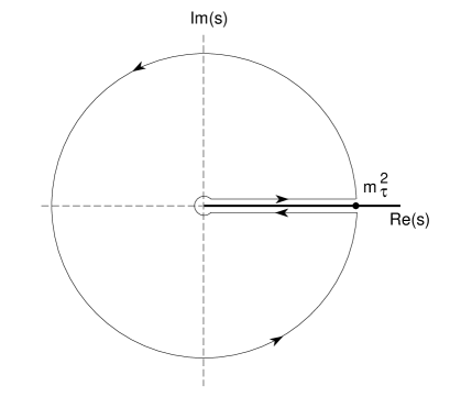
Figure 5: Integration contour in the complex s–plane, used to obtain Eq. (4.2)

Since the hadronic spectral functions are sensitive to the non-perturbative effects of QCD that bind quarks into hadrons, the integrand in Eq. (4.2) cannot be calculated at present from QCD. Nevertheless the integral itself can be calculated systematically by exploiting the analytic properties of the correlators $\Pi^{(J)}(s)$. They are analytic functions of $s$ except along the positive real $s$–axis, where their imaginary parts have discontinuities. $R_{\tau}$ can therefore be expressed as a contour integral in the complex $s$–plane running counter-clockwise around the circle $|s|=m_{\tau}^{2}$:

$$R_{\tau} \!\!\!\!\!= \!\!\!\!\!6\pi i\oint_{|s|=m_{\tau}^{2}}{ds\over m_{\tau}^{2}}\,\left(1-{s\over m_{\tau}^{2}}\right)^{2}$$

$$\!\!\!\!\!\times \!\!\!\!\!\left[\left(1+2{s\over m_{\tau}^{2}}\right)\Pi^{(0+1)}(s)-2{s\over m_{\tau}^{2}}\Pi^{(0)}(s)\right].$$

The advantage of expression (4.2) over (4.2) is that it requires the correlators only for complex $s$ of order $m_{\tau}^{2}$, which is significantly larger than the scale associated with non-perturbative effects in QCD. The short–distance OPE can therefore be used to organize the perturbative and non-perturbative contributions to the correlators into a systematic expansion [75] in powers of $1/s$. The possible uncertainties associated with the use of the OPE near the time-like axis are negligible in this case, because the integrand in (4.2) includes a factor $(1-s/m_{\tau}^{2})^{2}$, which provides a double zero at $s=m_{\tau}^{2}$, effectively suppressing the contribution from the region near the branch cut.

After evaluating the contour integral, $R_{\tau}$ can be expressed as an expansion in powers of $1/m_{\tau}^{2}$, with coefficients that depend only logarithmically on $m_{\tau}$:

$$R_{\tau}=3S_{EW}\left\{1+\delta_{EW}^{\prime}+\sum_{D=0,2,...}\delta^{(D)}\right\}.$$ (34)

The factors $S_{EW}=1.0194$ and $\delta_{EW}^{\prime}=0.0010$ contain the known electroweak corrections at the leading [2] and next-to-leading [76] logarithm approximation. The dimension–0 contribution, $\delta^{(0)}$, is the purely perturbative correction neglecting quark masses. It is given by [66, 67, 68, 69, 70, 71, 72]:

$$\delta^{(0)} \!\!\!= \!\!\!\sum_{n=1}K_{n}\,A^{(n)}(\alpha_{s})$$ (35)

$$\!\!\!= \!\!\!a_{\tau}+5.2023a_{\tau}^{2}+26.366a_{\tau}^{3}+\,{\cal O}(\alpha_{s}^{4})\,,$$

where $a_{\tau}\equiv\alpha_{s}(m_{\tau}^{2})/\pi$.

The dynamical coefficients $K_{n}$ regulate the perturbative expansion of $-s{d\over ds}\Pi^{(0+1)}(s)$ in the massless–quark limit [$s\Pi^{(0)}(s)=0$ for massless quarks]; they are known [77, 78, 79] to ${\cal O}(\alpha_{s}^{3})$: $K_{1}=1$; $K_{2}=1.6398$; $K_{3}(\overline{MS})=6.3711$. The kinematical effect of the contour integration is contained in the functions [70]

$$A^{(n)}(\alpha_{s}) \!\!\!\!= \!\!\!\!{1\over 2\pi i}\oint_{|s|=m_{\tau}^{2}}{ds\over s}\,\left({\alpha_{s}(-s)\over\pi}\right)^{n}$$ (36)

$$\!\!\!\!\times \!\!\!\!\left(1-2{s\over m_{\tau}^{2}}+2{s^{3}\over m_{\tau}^{6}}-{s^{4}\over m_{\tau}^{8}}\right),$$

which only depend on $\alpha_{s}(m_{\tau}^{2})$. Owing to the long running of the strong coupling along the circle, the coefficients of the perturbative expansion of $\delta^{(0)}$ in powers of $\alpha_{s}(m_{\tau}^{2})$ are larger than the direct $K_{n}$ contributions. This running effect can be properly resummed to all orders in $\alpha_{s}$ by fully keeping [70] the known three–loop–level calculation of the integrals $A^{(n)}(\alpha_{s})$.

The leading quark–mass corrections $\delta^{(2)}$ are known [69, 72, 80] to order $\alpha_{s}^{2}$. They are certainly tiny for the up and down quarks ($\delta^{(2)}_{ud}\sim-0.08\%$), but the correction from the strange quark mass is important for strange decays ($\delta^{(2)}_{us}\approx-19\%$). Nevertheless, because of the $|V_{us}|^{2}$ suppression, the effect on the total ratio $R_{\tau}$ is only $-(0.9\pm 0.2)\%$.

The leading non-perturbative contributions can be shown to be suppressed by six powers of the $\tau$ mass [66, 67, 68, 69], and are therefore very small. This fortunate fact is due to the phase–space factors in (4.2); their form is such that the leading $1/s^{2}$ corrections to $\Pi^{(1)}(s)$ do not survive the integration along the circle.

The numerical size of the non-perturbative corrections can be determined from the invariant–mass distribution of the final hadrons in $\tau$ decay [49]. Although the distributions themselves cannot be predicted at present, certain weighted integrals of the hadronic spectral functions can be calculated in the same way as $R_{\tau}$, and used to extract the non-perturbative contributions from the data themselves [49, 81]. The predicted suppression [66, 67, 68, 69] of the non-perturbative corrections has been confirmed by ALEPH [82] and CLEO [83]. The most recent ALEPH analysis [84] gives:

$$\delta_{\mbox{\rm\scriptsize NP}}\equiv\sum_{D\geq 4}\delta^{(D)}=(0.5\pm 1.1)\%\,,$$ (37)

in agreement with previous estimates [69].

Table 11: $\delta^{(0)}$ for different values of $\overline{\alpha}_{s}\equiv\alpha_{s}(m_{\tau}^{2})$ [72]

$\overline{\alpha}_{s}$	$\delta^{(0)}$	$\overline{\alpha}_{s}$	$\delta^{(0)}$
$0.24$	$0.118\pm 0.003$	$0.34$	$0.191\pm 0.009$
$0.26$	$0.132\pm 0.004$	$0.36$	$0.205\pm 0.010$
$0.28$	$0.146\pm 0.005$	$0.38$	$0.220\pm 0.012$
$0.30$	$0.161\pm 0.006$	$0.40$	$0.234\pm 0.013$
$0.32$	$0.176\pm 0.008$	$0.42$	$0.248\pm 0.013$

The QCD prediction for $R_{\tau}$ is then completely dominated by the perturbative contribution $\delta^{(0)}$; non-perturbative effects being smaller than the perturbative uncertainties from uncalculated higher–order corrections [72, 73, 74, 85]. Furthermore, as shown in Table 11, the result turns out to be very sensitive to the value of $\alpha_{s}(m_{\tau}^{2})$, allowing for an accurate determination of the fundamental QCD coupling.

The experimental value for $R_{\tau}$ can be obtained from the leptonic branching fractions or from the $\tau$ lifetime. The average of those determinations

$$R_{\tau}=3.649\pm 0.014\,,$$ (38)

corresponds to

$$\alpha_{s}(m_{\tau}^{2})=0.35\pm 0.03\,.$$ (39)

Once the running coupling constant $\alpha_{s}(s)$ is determined at the scale $m_{\tau}$, it can be evolved to higher energies using the renormalization group. The size of its error bar scales roughly as $\alpha_{s}^{2}$, and it therefore shrinks as the scale increases. Thus a modest precision in the determination of $\alpha_{s}$ at low energies results in a very high precision in the coupling constant at high energies. After evolution up to the scale $M_{Z}$, the strong coupling constant in (39) decreases to

$$\alpha_{s}(M_{Z}^{2})=0.122\pm 0.003\,,$$ (40)

in excellent agreement with the present LEP average [86] (without $R_{\tau}$) $\alpha_{s}(M_{Z}^{2})=0.122\pm 0.006$ and with a smaller error bar. The comparison of these two determinations of $\alpha_{s}$ in two extreme energy regimes, $m_{\tau}$ and $M_{Z}$, provides a beautiful test of the predicted running of the QCD coupling.

Using the measured invariant–mass distribution of the final hadrons, it is possible to evaluate the integral (4.2), with an arbitrary upper limit of integration $s_{0}\leq m_{\tau}$. The experimental $s_{0}$ dependence agrees well with the theoretical predictions [81] up to rather low values of $s_{0}$. Equivalently, from the measured $R_{\tau}(s_{0})$ distribution one obtains $\alpha_{s}(s_{0})$ as a function of the scale $s_{0}$ in good agreement with the running predicted at three–loop order by QCD [87].

With $\alpha_{s}(m_{\tau}^{2})$ fixed to the value in Eq. (39), the same theoretical framework gives definite predictions [69, 72] for the semi-inclusive $\tau$ decay widths $R_{\tau,V}$, $R_{\tau,A}$ and $R_{\tau,S}$, in good agreement with the experimental measurements [84, 88]. The analysis of these semi-inclusive quantities (and the associated invariant–mass distributions [81]) provides important information on several QCD parameters. For instance, $R_{\tau,V}-R_{\tau,A}$ is a pure non-perturbative quantity; basic QCD properties force the associated invariant–mass distribution to obey a series of chiral sum rules [49, 84]. The Cabibbo–suppressed width $R_{\tau,S}$ is very sensitive to the value of the strange quark mass [69], providing a direct and clean way of measuring $m_{s}$; a very preliminary value has been already presented at this workshop [88]. Last but not least, the measurement of the vector spectral function [89] Im$\Pi_{V}(s)$ helps to reduce the present uncertainties in fundamental QED quantities such as $\alpha(M_{Z})$ and $(g-2)_{\mu}$.

5 SEARCHING FOR NEW PHYSICS

5.1 Lepton–Number Violation

In the minimal SM with massless neutrinos, there is a separately conserved additive lepton number for each generation. All present data are consistent with this conservation law. However, there are no strong theoretical reasons forbidding a mixing among the different leptons, in the same way as happens in the quark sector. Many models in fact predict lepton–flavour or even lepton–number violation at some level. Experimental searches for these processes can provide information on the scale at which the new physics begins to play a significant role.

$K$, $\pi$ and $\mu$ decays, together with $\mu$–$e$ conversion, neutrinoless double beta decays and neutrino oscillation studies, have put already stringent limits [4] on lepton–flavour and lepton–number violating interactions. However, given the present lack of understanding of the origin of fermion generations, one can imagine different patterns of violation of this conservation law for different mass scales. Moreover, the larger mass of the $\tau$ opens the possibility of new types of decay which are kinematically forbidden for the $\mu$.

The present upper limits on lepton–flavour and lepton–number violating decays of the $\tau$ [4, 90] are in the range of $10^{-4}$ to $10^{-6}$, which is far away from the impressive bounds [4] obtained in $\mu$ decay [$Br(\mu^{-}\to e^{-}\gamma)<4.9\times 10^{-11},Br(\mu^{-}\to e^{-}e^{+}e^{-})<1.0\times 10^{-12},Br(\mu^{-}\to e^{-}\gamma\gamma)<7.2\times 10^{-11}\,$ (90% CL)]. With future $\tau$–decay samples of $10^{7}$ events per year, an improvement of two orders of magnitude would be possible.

The lepton–flavour violating couplings of the $Z$ boson have been investigated at LEP. The present ($95\%$ CL) limits are [91]:

$$\mbox{\rm Br}(Z\to e^{\pm}\mu^{\mp}) < 1.7\times 10^{-6};$$

$$\mbox{\rm Br}(Z\to e^{\pm}\tau^{\mp}) < 9.8\times 10^{-6};$$ (41)

$$\mbox{\rm Br}(Z\to\mu^{\pm}\tau^{\mp}) < 1.7\times 10^{-5}.$$

5.2 The Tau Neutrino

All observed $\tau$ decays are supposed to be accompanied by neutrino emission, in order to fulfil energy–momentum conservation requirements. The present data are consistent with the $\nu_{\tau}$ being a conventional sequential neutrino. Since taus are not produced by $\nu_{e}$ or $\nu_{\mu}$ beams, we know that $\nu_{\tau}$ is different from the electronic and muonic neutrinos, and a (90% CL) upper limit can be set on the couplings of the $\tau$ to $\nu_{e}$ and $\nu_{\mu}$ [92]:

$$|g_{\tau\nu_{e}}|<0.073\ ,\qquad|g_{\tau\nu_{\mu}}|<0.002\ .$$ (42)

These limits can be interpreted in terms of $\nu_{e}/\nu_{\mu}\to\nu_{\tau}$ oscillations, to exclude a region in the neutrino mass–difference and neutrino mixing–angle space. In the extreme situations of large $\delta m^{2}$ or maximal mixing, the limits are [92]:

$$\nu_{\mu}\to\nu_{\tau}:$$ (43)

$$\sin^{2}{2\theta_{\mu,\tau}}<0.004\qquad(\mbox{\rm large}\,\delta m_{\mu,\tau}^{2}),$$

$$\delta m_{\mu,\tau}^{2}<0.9\,\mbox{\rm eV}^{2}\quad\;\;(\sin^{2}{2\theta_{\mu,\tau}}=1);$$

$$\nu_{e}\to\nu_{\tau}:$$ (44)

$$\sin^{2}{2\theta_{e,\tau}}<0.12\qquad\;\;\,(\mbox{\rm large}\,\delta m_{e,\tau}^{2}),$$

$$\delta m_{e,\tau}^{2}<9\,\mbox{\rm eV}^{2}\qquad\;\,\,(\sin^{2}{2\theta_{e,\tau}}=1).$$

The new CHORUS [93] and NOMAD [94] experiments, presently running at CERN, and the future Fermilab E803 experiment are expected to improve the $\nu_{\mu}\to\nu_{\tau}$ oscillation limits by at least an order of magnitude.

LEP and SLC have confirmed [16] the existence of three (and only three) different light neutrinos, with standard couplings to the $Z$. However, no direct observation of $\nu_{\tau}$, that is, interactions resulting from neutrinos produced in $\tau$ decay, has been made so far.

The expected source of tau neutrinos in beam dump experiments is the decay of $D_{s}$ mesons produced by interactions in the dump; i.e., $p+N\to D_{s}+\cdots$ followed by the decays $D_{s}\to\tau^{-}\bar{\nu}_{\tau}$ and $\tau^{-}\to\nu_{\tau}+\cdots$ Several experiments [95] have searched for $\,\nu_{\tau}+N\to\tau^{-}+\cdots$ interactions with negative results; therefore, only an upper limit on the production of $\nu_{\tau}$’s has been obtained. The direct detection of the $\nu_{\tau}$ should be possible [96] at the LHC, thanks to the large charm production cross-section of this collider.

The possibility of a non-zero neutrino mass is obviously a very important question in particle physics [97]. There is no fundamental principle requiring a null mass for the neutrino. On the contrary, many extensions of the SM predict non-vanishing neutrino masses, which could have, in addition, important implications in cosmology and astrophysics. The strongest bound up to date is the preliminary ALEPH limit [9],

$$m_{\nu_{\tau}}\,<\,18.2\,\mbox{\rm MeV}\quad(95\%\,\mbox{\rm CL}),$$ (45)

obtained from a two–dimensional likelihood fit of the visible energy and the invariant–mass distribution of $\tau^{-}\to(3\pi)^{-}\nu_{\tau},(5\pi)^{-}\nu_{\tau}$ events.

For comparison, the present limits on the muon and electron neutrinos are [4] $m_{\nu_{\mu}}<170$ KeV (90% C.L.) and $m_{\nu_{e}}<15$ eV. Note, however, that in many models a mass hierarchy among different generations is expected, with the neutrino mass being proportional to some power of the mass of its charged lepton partner. Assuming for instance the fashionable relation $\,m_{\nu_{\tau}}/m_{\nu_{e}}\sim(m_{\tau}/m_{e})^{2}$, the bound (45) would be equivalent to a limit of 1.5 eV for $m_{\nu_{e}}$. A relatively crude measurement of $m_{\nu_{\tau}}$ may then imply strong constraints on neutrino–mass model building.

More stringent (but model–dependent) bounds on $m_{\nu_{\tau}}$ can be obtained from cosmological considerations. A stable neutrino (or an unstable one with a lifetime comparable to or longer than the age of the Universe) must not overclose the Universe. Therefore, measurements of the age of the Universe exclude stable neutrinos in the range [98, 99] 200 eV $<m_{\nu}<$ 2 GeV. Unstable neutrinos with lifetimes longer than 300 sec could increase the expansion rate of the Universe, spoiling the successful predictions for the primordial nucleosynthesis of light isotopes in the early universe [100]; the mass range 0.5 MeV $<m_{\nu_{\tau}}<$ 30 MeV has been excluded in that case [100, 101, 102, 103, 104]. For neutrinos of any lifetime decaying into electromagnetic daughter products, it is possible to exclude the same mass range, combining the nucleosynthesis constraints with limits based on the supernova SN 1987A and on BEBC data [103, 104]. Light neutrinos ($m_{\nu_{\tau}}<100$ keV) decaying through $\nu_{\tau}\to\nu_{\mu}+G^{0}$, are also excluded by the nucleosynthesis constraints, if their lifetime is shorter than $10^{-2}$ sec [102].

The astrophysical and cosmological arguments lead indeed to quite stringent limits; however, they always involve (plausible) assumptions which could be relaxed in some physical scenarios [105, 106]. For instance, in deriving the abundance of massive $\nu_{\tau}$’s at nucleosynthesis, it is always assumed that tau neutrinos annihilate at the rate predicted by the SM. A $\nu_{\tau}$ mass in the few MeV range (i.e. the mass sensitivity which can be achieved in the foreseeable future) could have a host of interesting astrophysical and cosmological consequences [104]: relaxing the big-bang nucleosynthesis bound to the baryon density and the number of neutrino species; allowing big-bang nucleosynthesis to accommodate a low ($<20\%$) ⁴He mass fraction or high ($>10^{-4}$) deuterium abundance; improving significantly the agreement between the cold dark matter theory of structure formation and observations [107]; and helping to explain how type II supernova explode.

The electromagnetic structure of the $\nu_{\tau}$ can be tested through the process $e^{+}e^{-}\to\nu_{\tau}\bar{\nu}_{\tau}\gamma$. The combined data from PEP and PETRA implies [108] the following $90\%$ CL upper bounds on the magnetic moment and charge radius of the $\nu_{\tau}$ ($\mu_{B}\equiv e\hbar/2m_{e}$): $|\mu(\nu_{\tau})|<4\times 10^{-6}\,\mu_{B}$; $<r^{2}>(\nu_{\tau})<2\times 10^{-31}\,\mbox{\rm cm}^{2}$. A better limit on the $\nu_{\tau}$ magnetic moment,

$$|\mu(\nu_{\tau})|<5.4\times 10^{-7}\,\mu_{B}\quad(90\%\,\mbox{\rm CL}),$$ (46)

has been placed by the BEBC experiment [109], by searching for elastic $\nu_{\tau}e$ scattering events, using a neutrino beam from a beam dump which has a small $\nu_{\tau}$ component.

A big $\nu_{\tau}$ magnetic moment of about $10^{-6}\mu_{B}$ has been suggested, in order to make the $\tau$ neutrino an acceptable cold dark matter candidate. For this to be the case, however, the $\nu_{\tau}$ mass should be in the range 1 MeV $<m_{\nu_{\tau}}<$ 35 MeV [110]. The same region of $m_{\nu_{\tau}}$ has been suggested in trying to understand the baryon–antibaryon asymmetry of the universe [111].

5.3 Dipole Moments

Owing to their chiral changing structure, the electroweak dipole moments may provide important insights on the mechanism responsible for mass generation. In general, one expects [14] that a fermion of mass $m_{f}$ (generated by physics at some scale $M\gg m_{f}$) will have induced dipole moments proportional to some power of $m_{f}/M$. Therefore, heavy fermions such as the $\tau$ should be a good testing ground for this kind of effects. Of special interest are the electric and weak dipole moments, $d^{\gamma,Z}_{\tau}$, which violate $T$ and $P$ invariance; they constitute a good probe of CP violation.

The more stringent (95% CL) limits on the anomalous magnetic moment and the electric dipole moment of the $\tau$ have been derived from an analysis of the $Z\to\tau^{+}\tau^{-}$ decay width [112], assuming that all other couplings take their SM values:

$$-0.004<a^{\gamma}_{\tau}<0.006\ ,$$

$$|d^{\gamma}_{\tau}|<2.7\times 10^{-17}\,e\,\mbox{\rm cm}.$$ (47)

These limits would be invalidated in the presence of any CP–conserving contribution to $\Gamma(Z\to\tau^{+}\tau^{-})$ interfering destructively with the SM amplitude.

Slightly weaker bounds have been extracted from the decay $Z\to\tau^{+}\tau^{-}\gamma$ [113] (95% CL):

$$|a^{\gamma}_{\tau}|<0.0104\ ,\qquad|d^{\gamma}_{\tau}|<5.8\times 10^{-17}\,e\,\mbox{\rm cm},$$ (48)

and from PEP and PETRA data [114, 115, 116]: $|a^{\gamma}_{\tau}|(35\,\mbox{\rm GeV})<0.023$ (95% CL), $|d^{\gamma}_{\tau}|(35\,\mbox{\rm GeV})<1.6\times 10^{-16}\,e$ cm (90% CL).

In the SM, $|d^{\gamma}_{\tau}|$ vanishes, while the overall value of $a^{\gamma}_{\tau}$ is dominated by the second order QED contribution [117], $a^{\gamma}_{\tau}\approx\alpha/2\pi$. Including QED corrections up to O($\alpha^{3}$), hadronic vacuum polarization contributions and the corrections due to the weak interactions (which are a factor 380 larger than for the muon), the tau anomalous magnetic moment has been estimated to be [118, 119]

$$a^{\gamma}_{\tau}\big{|}_{\mbox{\rm\scriptsize th}}\,=\,(1.1773\pm 0.0003)\times 10^{-3}\,.$$ (49)

The first direct limit on the weak anomalous magnetic moment has been obtained by L3, by using correlated azimuthal asymmetries of the $\tau^{+}\tau^{-}$ decay products [120]. The preliminary (95% CL) result of this analysis is [121]:

$$-0.016<a^{Z}_{\tau}<0.011\ .$$ (50)

The possibility of a CP–violating weak dipole moment of the $\tau$ has been investigated at LEP, by studying $T$–odd triple correlations [122, 123] of the final $\tau$–decay products in $Z\to\tau^{+}\tau^{-}$ events. The present (95% CL) limits are [113]:

$$|\mbox{\rm Re}\,d^{Z}_{\tau}(M_{Z}^{2})|\leq 3.6\times 10^{-18}\,e\,\mbox{\rm cm},$$

$$|\mbox{\rm Im}\,d^{Z}_{\tau}(M_{Z}^{2})|\leq 1.1\times 10^{-17}\,e\,\mbox{\rm cm}.$$ (51)

These limits provide useful constraints on different models of CP violation [122, 124, 125, 126].

T–odd signals can be also generated through a relative phase between the vector and axial-vector couplings of the $Z$ to the $\tau^{+}\tau^{-}$ pair [35], i.e. $\mbox{\rm Im}(v_{\tau}a_{\tau}^{*})\not=0$. This effect, which in the SM appears [127] at the one-loop level through absorptive parts in the electroweak amplitudes, gives rise [35] to a spin–spin correlation associated with the transverse (within the production plane) and normal (to the production plane) polarization components of the two $\tau$’s. A preliminary measurement of these transverse spin correlations has been reported by ALEPH [128].

5.4 CP Violation

In the three–generation SM, the violation of the CP symmetry originates from the single phase naturally occurring in the quark mixing matrix [129] . Therefore, CP violation is predicted to be absent in the lepton sector (for massless neutrinos). The present experimental observations are in agreement with the SM; nevertheless, the correctness of the Kobayashi—Maskawa mechanism is far from being proved. Like fermion masses and quark mixing angles, the origin of the Kobayashi—Maskawa phase lies in the most obscure part of the SM Lagrangian: the scalar sector. Obviously, CP violation could well be a sensitive probe for new physics.

Up to now, CP violation in the lepton sector has been investigated mainly through the electroweak dipole moments. Violations of the CP symmetry could also happen in the $\tau$ decay amplitude. In fact, the possible CP–violating effects can be expected to be larger in $\tau$ decay than in $\tau^{+}\tau^{-}$ production [130]. Since the decay of the $\tau$ proceeds through a weak interaction, these effects could be ${\cal O}(1)$ or ${\cal O}(10^{-3})$, if the leptonic CP violation is weak or milliweak [130].

With polarized electron (and/or positron) beams, one could use the longitudinal polarization vectors of the incident leptons to construct T–odd rotationally invariant products. CP could be tested by comparing these T–odd products in $\tau^{-}$ and $\tau^{+}$ decays. In the absence of beam polarization, CP violation could still be tested through $\tau^{+}\tau^{-}$ correlations. In order to separate possible CP–odd effects in the $\tau^{+}\tau^{-}$ production and in the $\tau$ decay, it has been suggested to study the final decays of the $\tau$–decay products and build the so-called stage–two spin–correlation functions [131]. For instance, one could study the chain process $e^{+}e^{-}\to\tau^{+}\tau^{-}\to(\rho^{+}\bar{\nu}_{\tau})(\rho^{-}\nu_{\tau})\to(\pi^{+}\pi^{0}\bar{\nu}_{\tau})(\pi^{-}\pi^{0}\nu_{\tau})$. The distribution of the final pions provides information on the $\rho$ polarization, which allows to test for possible CP–violating effects in the $\tau\to\rho\nu_{\tau}$ decay.

CP violation could also be tested through rate asymmetries, i.e. comparing the partial fractions $\Gamma(\tau^{-}\to X^{-})$ and $\Gamma(\tau^{+}\to X^{+})$. However, this kind of signal requires the presence of strong final–state interactions in the decay amplitude. Another possibility would be to study T–odd (CPT–even) asymmetries in the angular distributions of the final hadrons in semileptonic $\tau$ decays [132]. Explicit studies of the decay modes $\tau^{-}\to K^{-}\pi^{-}\pi^{+},\pi^{-}K^{-}K^{+}$ [133] and $\tau^{-}\to\pi^{-}\pi^{-}\pi^{+}$ [134] show that sizeable CP–violating effects could be generated in some models of CP violation involving several Higgs doublets or left–right symmetry.

6 SUMMARY

The flavour structure of the SM is one of the main pending questions in our understanding of weak interactions. Although we do not know the reason of the observed family replication, we have learned experimentally that the number of SM fermion generations is just three (and no more). Therefore, we must study as precisely as possible the few existing flavours to get some hints on the dynamics responsible for their observed structure.

The $\tau$ turns out to be an ideal laboratory to test the SM. It is a lepton, which means clean physics, and moreover it is heavy enough to produce a large variety of decay modes. Naïvely, one would expect the $\tau$ to be much more sensitive than the $e$ or the $\mu$ to new physics related to the flavour and mass–generation problems.

QCD studies can also benefit a lot from the existence of this heavy lepton, able to decay into hadrons. Owing to their semileptonic character, the hadronic $\tau$ decays provide a powerful tool to investigate the low–energy effects of the strong interactions in rather simple conditions.

Our knowledge of the $\tau$ properties has been considerably improved during the last few years. Lepton universality has been tested to rather good accuracy, both in the charged and neutral current sectors. The Lorentz structure of the leptonic $\tau$ decays is certainly not determined, but begins to be experimentally explored. The quality of the hadronic data has made possible to perform quantitative QCD tests and determine the strong coupling constant very accurately. Searches for non-standard phenomena have been pushed to the limits that the existing data samples allow to investigate.

At present, all experimental results on the $\tau$ lepton are consistent with the SM. There is, however, large room for improvements. Future $\tau$ experiments will probe the SM to a much deeper level of sensitivity and will explore the frontier of its possible extensions.

References

- [1] Proc. Third Workshop on Tau Lepton Physics (Montreux, 1994), ed. L. Rolandi, Nucl. Phys. B (Proc. Suppl.) 40 (1995).
- [2] W.J. Marciano and A. Sirlin, Phys. Rev. Lett. 61 (1988) 1815.
- [3] A. Pich, Tau Physics, in Heavy Flavours, eds. A.J. Buras and M. Lindner, Advanced Series on Directions in High Energy Physics – Vol. 10 (World Scientific, Singapore, 1992), p. 375.
- [4] Particle Data Group, Review of Particle Properties, Phys. Rev. D54 (1996) 1.
- [5] H.G. Evans, these proceedings.
- [6] P. Weber, these proceedings.
- [7] L. Rolandi, these proceedings.
- [8] D. Buskulic et al (ALEPH), Phys. Lett. B349 (1995) 585.
- [9] L. Passalacqua, these proceedings.
- [10] W.J. Marciano and A. Sirlin, Phys. Rev. Lett. 71 (1993) 3629.
- [11] R. Decker and M. Finkemeier, Nucl. Phys. B438 (1995) 17; in [1], p. 453.
-
[12]
D.I. Britton et al, Phys. Rev. Lett. 68 (1992) 3000;
G. Czapek et al, Phys. Rev. Lett. 70 (1993) 17. -
[13]
C. Albajar et al (UA1), Z. Phys. C44 (1989) 15;
J. Alitti et al (UA2), Phys. Lett. B280 (1992) 137;
F. Abe et al (CDF), Phys. Rev. Lett. 68 (1992) 3398; 69 (1992) 28. - [14] W.J. Marciano, in [1], p. 3.
- [15] J.M. Roney, these proceedings.
- [16] The LEP Electroweak Working Group and the SLD Heavy Flavour Group, A Combination of Preliminary LEP and SLD Electroweak Measurements and Constraints on the Standard Model, CERN preprint LEPEWWG/96-02 (30 July 1996).
- [17] R. Alemany et al, Nucl. Phys. B379 (1992) 3.
- [18] D. Buskulic et al (ALEPH), Phys. Lett. B321 (1994) 168.
- [19] M. Acciarri et al (L3), Phys. Lett. B377 (1996) 313.
- [20] P. Vilain et al (CHARM II), Phys. Lett. B335 (1994) 246.
- [21] P. Vilain et al (CHARM II), Phys. Lett. B320 (1994) 203.
- [22] L. Michel, Proc. Phys. Soc. A63 (1950) 514; 1371.
-
[23]
C. Bouchiat and L. Michel, Phys. Rev. 106 (1957) 170;
T. Kinoshita and A. Sirlin, Phys. Rev. 107 (1957) 593; 108 (1957) 844. - [24] F. Scheck, Leptons, Hadrons and Nuclei (North-Holland, Amsterdam, 1983); Phys. Rep. 44 (1978) 187.
- [25] W. Fetscher, H.-J. Gerber and K.F. Johnson, Phys. Lett. B173 (1986) 102.
- [26] W. Fetscher and H.-J. Gerber, Precision Measurements in Muon and Tau Decays, in Precision Tests of the Standard Electroweak Model, ed. P. Langacker, Advanced Series on Directions in High Energy Physics – Vol. 14 (World Scientific, Singapore, 1995), p. 657.
- [27] A. Pich and J.P. Silva, Phys. Rev. D52 (1995) 4006.
- [28] A. Rougé, Results on Neutrino from Colliders, Proc. XXX Rencontre de Moriond, Dark Matter in Cosmology, Clocks and Tests of Fundamental Laws, eds. B. Guiderdoni et al (Editions Frontières, Gif-sur-Yvette, 1995) p. 247.
- [29] C. Jarlskog, Nucl. Phys. 75 (1966) 659.
- [30] W. Fetscher, Phys. Lett. 140B (1984) 117.
-
[31]
Y.S. Tsai, Phys. Rev. D4 (1971) 2821;
S. Kawasaki, T. Shirafuji and S.Y. Tsai, Progr. Theor. Phys. 49 (1973) 1656. - [32] S.-Y. Pi and A.I. Sanda, Ann. Phys., NY 106 (1977) 171.
-
[33]
C.A. Nelson, Phys. Rev. D43 (1991) 1465;
Phys. Rev. Lett. 62 (1989) 1347; Phys. Rev. D40 (1989) 123
[Err: D41 (1990) 2327];
S. Goozovat and C.A. Nelson, Phys. Rev. D44 (1991) 2818; Phys. Lett. B267 (1991) 128 [Err: B271 (1991) 468]. - [34] W. Fetscher, Phys. Rev. D42 (1990) 1544.
- [35] J. Bernabéu, A. Pich and N. Rius, Phys. Lett. B257 (1991) 219.
- [36] M. Davier et al, Phys. Lett. B306 (1993) 411.
- [37] J. Quigley, these proceedings.
- [38] A. Stahl and H. Voss, BONN-HE-96-02.
- [39] D. Buskulic et al (ALEPH), Phys. Lett. B346 (1995) 379.
- [40] M. Chadha, these proceedings.
- [41] W. Lohmann and J. Raab, Charged Current Couplings in Decay, DESY 95-188.
- [42] A. Stahl, Phys. Lett. B324 (1994) 121.
- [43] H.B. Thacker and J.J. Sakurai, Phys. Lett. 36B (1971) 103.
-
[44]
F.J. Gilman and S.H. Rhie, Phys. Rev. D31 (1985) 1066;
F.J. Gilman and D.H. Miller, Phys. Rev. D17 (1978) 1846;
F.J. Gilman, Phys. Rev. D35 (1987) 3541. - [45] J.H. Kühn and A. Santamaría, Z. Phys. C48 (1990) 445.
- [46] S.I. Eidelman and V.N. Ivanchenko, Phys. Lett. B257 (1991) 437; in [1], p. 131.
- [47] S. Narison and A. Pich, Phys. Lett. B304 (1993) 359.
- [48] S. Eidelman and V. Ivanchenko, these proceedings.
- [49] A. Pich, QCD Tests from Tau Decay Data, in Proc. Tau-Charm Factory Workshop (SLAC, California, 1989), ed. L.V. Beers, SLAC-Report-343 (1989), p. 416.
- [50] J. Gasser and H. Leutwyler, Nucl. Phys. B250 (1985) 465.
- [51] A. Pich, Rep. Prog. Phys. 58 (1995) 563.
- [52] G. Ecker, Prog. Part. Nucl. Phys. 35 (1995) 1.
- [53] Colangelo, M. Finkemeier and R. Urech, Phys. Rev. D54 (1996) 4403.
- [54] H. Davoudiasl and M.B. Wise, Phys. Rev. D53 (1996) 2523.
- [55] R. Fischer, J. Wess and F. Wagner, Z. Phys. C3 (1980) 313.
- [56] A. Pich, Phys. Lett. B196 (1987) 561.
- [57] J.J. Gómez–Cadenas, C.M. González–García and A. Pich, Phys. Rev. D42 (1990) 3093.
-
[58]
R. Decker et al, Z. Phys. C58 (1993) 445;
M. Finkemeier and E. Mirkes, Z. Phys.C69 (1996) 243;
R. Decker, M. Finkemeier and E. Mirkes, Phys. Rev. D50 (1994) 6863;
M. Finkemeier et al, these proceedings. - [59] R. Decker et al, Z. Phys. C70 (1996) 247.
- [60] S. Jadach et al, Comput. Phys. Commun. 64 (1991) 275; 76 (1993) 361.
-
[61]
T.E. Coan et al, CLEO CONF 96-15;
V. Shelkov, these proceedings. - [62] G. Ecker et al, Nucl. Phys. B321 (1989) 311; Phys. Lett. 233B (1989) 425.
- [63] H. Neufeld and H. Rupertsberger, Z. Phys. C68 (1995) 91.
- [64] F. Guerrero and A. Pich, to be published.
-
[65]
J.H. Kühn and E. Mirkes, Z. Phys. C56 (1992) 661
[Err: C67 (1995) 364]; Phys. Lett. B286 (1992) 281;
G. Colangelo et al, these proceedings. - [66] E. Braaten, Phys. Rev. Lett. 60 (1988) 1606; Phys. Rev. D39 (1989) 1458.
- [67] S. Narison and A. Pich, Phys. Lett. B211 (1988) 183.
- [68] A. Pich, Hadronic Tau-Decays and QCD, Proc. Workshop on Tau Lepton Physics (Orsay, 1990), eds. M. Davier and B. Jean-Marie (Ed. Frontières, Gif-sur-Yvette, 1991), p. 321.
- [69] E. Braaten, S. Narison and A. Pich, Nucl. Phys. B373 (1992) 581.
- [70] F. Le Diberder and A. Pich, Phys. Lett. B286 (1992) 147.
- [71] A. Pich, QCD Predictions for the Tau Hadronic Width and Determination of , Proc. Second Workshop on Tau Lepton Physics (Ohio, 1992), ed. K.K. Gan (World Scientific, Singapore, 1993), p. 121.
- [72] A. Pich, Nucl. Phys. B (Proc. Suppl.) 39B,C (1995) 326.
- [73] S. Narison, in [1], p. 47.
- [74] E. Braaten, these proceedings.
- [75] M.A. Shifman, A.L. Vainshtein and V.I. Zakharov, Nucl. Phys. B147 (1979) 385; 448; 519.
- [76] E. Braaten and C.S. Li, Phys. Rev. D42 (1990) 3888.
-
[77]
K.G. Chetyrkin, A.L. Kataev and F.V. Tkachov, Phys. Lett. 85B (1979) 277;
M. Dine and J. Sapirstein, Phys. Rev. Lett. 43 (1979) 668;
W. Celmaster and R. Gonsalves, Phys. Rev. Lett. 44 (1980) 560. - [78] S.G. Gorishny, A.L. Kataev and S.A. Larin, Phys. Lett. B259 (1991) 144.
- [79] L.R. Surguladze and M.A. Samuel, Phys. Rev. Lett. 66 (1991) 560.
- [80] K.G. Chetyrkin and A. Kwiatkowski, Z. Phys. C59 (1993) 525.
- [81] F. Le Diberder and A. Pich, Phys. Lett. B289 (1992) 165.
- [82] D. Buskulic et al (ALEPH), Phys. Lett. B307 (1993) 209.
- [83] T. Coan et al (CLEO), Phys. Lett. B356 (1995) 580.
- [84] A. Höcker, these proceedings.
- [85] P.A. Raczka, these proceedings.
- [86] S. Bethke, Experimental Tests of Asymptotic Freedom, Proc. QCD’96 (Montpellier, 1996), ed. S. Narison [hep-ex/9609014].
- [87] M. Girone and M. Neubert, Phys. Rev. Lett. 76 (1996) 3061.
- [88] M. Davier, these proceedings.
- [89] R. Alemany, these proceedings.
- [90] K.K. Gan, these proceedings.
- [91] R. Akers et al (OPAL), Z. Phys. C67 (1995) 555.
- [92] N. Ushida et al (Fermilab E531), Phys. Rev. Lett. 57 (1986) 2897.
- [93] G. Gregoire, these proceedings.
- [94] A. Cardini, these proceedings.
- [95] M. Talebzadeh et al (BEBC WA66), Nucl. Phys. B291 (1987) 503; and references therein.
-
[96]
A. De Rújula and R. Rückl, Proc. of the ECFA-CERN
Workshop on LHC in the LEP Tunnel (Lausanne-Geneva, 1984)
CERN 84-10, Vol.II, p. 571;
A. De Rújula, E. Fernández and J.J. Gómez–Cadenas, Nucl. Phys. B405 (1993) 80. - [97] P. Langacker, these proceedings.
-
[98]
S.S. Gerstein and Ya.B. Zeldovich, JETP Lett. 15 (1972) 174;
R. Cowsik and J. McClelland, Phys. Rev. Lett. 29 (1972) 669;
R.A. Syunaev and Ya.B. Zeldovich, Pis’ma Astron. Zh. 6 (1980) 451. - [99] B.W. Lee and S. Weinberg, Phys. Rev. Lett. 39 (1977) 165.
- [100] E.W. Kolb et al, Phys. Rev. Lett. 67 (1991) 533.
- [101] A.D. Dolgov and I.Z. Rothstein, Phys. Rev. Lett. 71 (1993) 476.
- [102] M. Kawasaki et al, Nucl. Phys. B419 (1994) 105.
- [103] S. Dodelson, G. Gyuk and M.S. Turner, Phys. Rev. D49 (1994) 5068.
- [104] G. Gyuk and M.S. Turner, in [1], p. 557.
- [105] R.N. Mohapatra and S. Nussinov, Phys. Rev. D51 (1995) 3843.
- [106] B.D. Fields, K. Kainulainen and K.A. Olive, CERN-TH/95-335.
- [107] S. Dodelson, G. Gyuk and M.S. Turner, Phys. Rev. Lett. 72 (1994) 3754.
- [108] H. Grotch and R.W. Robinett, Z. Phys. C39 (1988) 553.
- [109] A.M. Cooper-Sarkar et al (BEBC), Phys. Lett. B280 (1992) 153.
- [110] G.F. Giudice, Phys. Lett. B251 (1990) 460.
- [111] A.G. Cohen, D.B. Kaplan and A.E. Nelson, Phys. Lett. B263 (1991) 86.
-
[112]
R. Escribano and E. Masso, Phys. Lett. B301 (1993) 419;
Nucl. Phys. B429 (1994) 19;
hep-ph/9609423. - [113] N. Wermes, these proceedings.
- [114] D.J. Silverman and G.L. Shaw, Phys. Rev. D27 (1983) 1196.
- [115] R. Marshall, Rep. Prog. Phys. 52 (1989) 1329.
- [116] F. del Aguila and M. Sher, Phys. Lett. B252 (1990) 116.
- [117] J.S. Schwinger, Phys. Rev. 73 (1948) 416.
- [118] S. Narison, J. Phys. G: Nucl. Phys. 4 (1978) 1849.
- [119] M.A. Samuel, G. Li and R. Mendel, Phys. Rev. Lett. 67 (1991) 668.
- [120] J. Bernabéu, G.A. González–Sprinberg and J. Vidal, Phys. Lett. B326 (1994) 168.
- [121] E. Sánchez, these proceedings.
- [122] W. Bernreuther and O. Nachtmann, Phys. Rev. Lett. 63 (1989) 2787 [Err: 64 (1990) 1072].
- [123] W. Bernreuther et al, Z. Phys. C52 (1991) 567; Phys. Rev. D48 (1993) 78.
- [124] W. Bernreuther et al, Z. Phys. C43 (1989) 117.
- [125] A. De Rújula et al, Nucl. Phys. B357 (1991) 311.
- [126] J. Körner et al, Z. Phys. C49 (1991) 447.
- [127] J. Bernabéu and N. Rius, Phys. Lett. B232 (1989) 127.
- [128] F. Sánchez, these proceedings.
- [129] M. Kobayashi and T. Maskawa, Prog. Theor. Phys 42 (1973) 652.
- [130] Y.S. Tsai, Phys. Rev. D51 (1995) 3172; these proceedings.
-
[131]
C.A. Nelson et al, Phys. Rev. D50 (1994) 4544;
C. A. Nelson, these proceedings. - [132] M. Finkemeier and E. Mirkes, Decay Rates, Structure Functions and New Physics Effects in Hadronic Tau Decays, Proc. Workshop on the Tau/Charm Factory (Argonne, 1995), ed. J. Repond, AIP Conf. Proc. No. 349 (New York, 1996) p. 119.
- [133] U. Kilian et al, Z. Phys. C62 (1994) 413.
- [134] S.Y. Choi, K. Hagiwara and M. Tanabashi, Phys. Rev. D52 (1995) 1614.