1 Introduction
Consider the full fermion propagator
in the presence of a dynamically broken chiral symmetry in a gauge
theory with no explicit fermion masses.
S − 1 ( p ) = Z ( p 2 ) p / − Σ ( p 2 ) {S}^{-1}(p)=Z({p}^{2}){p}\!\!\!{/}-\Sigma({p}^{2}) (1)
Σ ( p 2 ) Σ superscript 𝑝 2 \Sigma({p}^{2}) e − 1 / b g 2 superscript 𝑒 1 𝑏 superscript 𝑔 2 {e}^{-1/b{g}^{2}} g 𝑔 g b 𝑏 b [1 ] . We quote from their work.
To lowest order
this approximation can be described as follows. Amplitudes that do
not vanish to all orders of perturbation theory are given by their
free-field values. For example, the amplitude
Z ( p 2 ) 𝑍 superscript 𝑝 2 Z(p^{2}) 1 Z ( p 2 ) = 1 𝑍 superscript 𝑝 2 1 Z({p}^{2})=1 λ = e − 1 / b g 2 𝜆 superscript 𝑒 1 𝑏 superscript 𝑔 2 \lambda={e}^{-1/b{g}^{2}} Σ ( p 2 ) Σ superscript 𝑝 2 \Sigma({p}^{2}) g n e − 1 / b g 2 superscript 𝑔 𝑛 superscript 𝑒 1 𝑏 superscript 𝑔 2 {g}^{n}{e}^{-1/b{g}^{2}} n > 0 𝑛 0 n>0 g 2 superscript 𝑔 2 g^{2} λ = e − 1 / b g 2 𝜆 superscript 𝑒 1 𝑏 superscript 𝑔 2 \lambda={e}^{-1/b{g}^{2}}
One result of this work is a popular
formula relating the (pseudo)Goldstone boson decay constant to the
fermion mass function, which has been widely used in studies of QCD
and other theories with chiral symmetry breaking. This formula is
found to be in good agreement with a more sophisticated
Bethe-Salpeter approach [2 ] .
Since the Ward identities are satisfied the idea of DPT at lowest
order can be extended to a Lagrangian-based GNC (gauged nonlocal
constituent) relativistic quark model [3 ] which preserves the
chiral structure of QCD. The Lagrangian must be nonlocal to
incorporate the momentum dependent mass. The GNC model reproduced the
Pagels-Stokar decay constant formula, and when expanded to
order p 4 superscript 𝑝 4 p^{4} [4 ] . The incorporation of this momentum dependence
represents an improvement over constant mass quark models of the
Nambu-Jona-Lasino type. But the question remains, why does a free
quark model represent low energy QCD dynamics as well as it does? For
example at the level of the quark propagator, how can the momentum
dependence of
Z ( p 2 ) 𝑍 superscript 𝑝 2 Z(p^{2}) 1
By using the auxiliary field method we shall provide a systematic
derivation of DPT and the GNC quark model from a gauge theory. The
connection with DPT is made by introducing auxiliary fields only for
those quark bilinears which define purely nonperturbative amplitudes.
The auxiliary fields introduced are thus chirality changing, and they
may also carry color or fermion number. The effective theory at
lowest order in a loop expansion will correspond to the lowest order
in DPT, and the origin of the GNC quark model is made clear.
We shall
also find a set of ladder SD equations which are all homogeneous
equations in the auxiliary fields. It may be noted
that these SD equations treat all the possible quark mass functions
in the various channels, including Σ ( p ) Σ 𝑝 \Sigma(p) q ¯ q ¯ 𝑞 𝑞 \overline{q}q Σ ( p ) Σ 𝑝 \Sigma(p) Z ( p ) = 1 𝑍 𝑝 1 Z(p)=1 Z ( p ) = 1 𝑍 𝑝 1 Z(p)=1
We shall deal with the problem of gauge boson self-interactions by
studying a strongly interacting U ( N c ) 𝑈 subscript 𝑁 𝑐 U(N_{c}) S U ( N c ) 𝑆 𝑈 subscript 𝑁 𝑐 SU(N_{c}) N f subscript 𝑁 𝑓 N_{f} U ( N c ) 𝑈 subscript 𝑁 𝑐 U(N_{c}) g 𝑔 g g 1 subscript 𝑔 1 g_{1} S U ( N c ) 𝑆 𝑈 subscript 𝑁 𝑐 SU(N_{c}) U ( 1 ) 𝑈 1 U(1) q ¯ q ¯ 𝑞 𝑞 \overline{q}q g 𝑔 g g 1 subscript 𝑔 1 g_{1} g 𝑔 g g 𝑔 g g 1 subscript 𝑔 1 g_{1} U ( 1 ) 𝑈 1 U(1) g 𝑔 g g 1 subscript 𝑔 1 g_{1} g 𝑔 g g 𝑔 g S U ( N c ) 𝑆 𝑈 subscript 𝑁 𝑐 SU(N_{c})
Our approach will also shed some light on the concept of duality in
the description of low energy chiral dynamics. This is related to
the observation that the low energy chiral Lagrangian to order p 4 superscript 𝑝 4 p^{4} do not include vector or axial vector
degrees of freedom. Instead we will have scalar and tensor fields,
some of which have color and/or diquark quantum numbers. The lowest
order in a loop expansion involving all massive degrees of freedom
corresponds to setting all the non-Goldstone-boson degrees of freedom
in the various auxiliary fields to their vacuum values. The fact that
we are not required to fix vector or axial-vector degrees of freedom
then suggests how it is that a constituent quark model can reproduce
the effects of vector or axial-vector degrees of freedom.
Our basic result is that the perturbative expansion of a nonabelian
gauge theory may be reorganized in such a way that the lowest order
in the new loop expansion coincides with a previously studied and
successful quark model of low energy chiral dynamics. Instead of
being put in by hand, the quark mass function emerges from the
dynamics. Also the quark model now exists in a framework of a loop
expansion in which corrections, at least in principle, may be
systematically worked out. Such a process was implied but not
specified in the original proposal for DTP. As one example the
phenomenological effects of various scalar and diquark degrees of
freedom could be explored in the context of a quark model, without
fear of double counting degrees of freedom.
In the next two sections we shall derive generating functionals
without and with, respectively, the effects of cubic and quartic
gauge couplings. The latter case is significantly more complicated,
and it will be carried out by introducing two sets of auxiliary
fields. In the next section we also show how the (pseudo)Goldstone
degrees of freedom may be retained for a description of low energy
physics.
2 Low energy theory
Due to our study of U ( N c ) 𝑈 subscript 𝑁 𝑐 U(N_{c}) S U ( N c ) 𝑆 𝑈 subscript 𝑁 𝑐 SU(N_{c})
e i W [ J ] superscript 𝑒 𝑖 𝑊 delimited-[] 𝐽 \displaystyle e^{iW[J]} = \displaystyle= ∫ 𝒟 ψ 𝒟 ψ ¯ exp i { ∫ d 4 x ψ ¯ ( i ∂ / + J ) ψ \displaystyle\int{\cal D}\psi{\cal D}\overline{\psi}{\rm exp}i{\bigg{\{}}{\int}d^{4}x\overline{\psi}(i\partial\!\!\!/+J){\psi} (2)
+ i 2 g 2 2 ∫ d 4 x d 4 y G μ ν ( x , y ) [ ψ ¯ α i ( x ) ( λ a 2 ) α β γ μ ψ β i ( x ) ] [ ψ ¯ α ′ j ( y ) ( λ a 2 ) α ′ β ′ γ ν ψ β ′ j ( y ) ] superscript 𝑖 2 superscript 𝑔 2 2 superscript 𝑑 4 𝑥 superscript 𝑑 4 𝑦 subscript 𝐺 𝜇 𝜈 𝑥 𝑦 delimited-[] subscript superscript ¯ 𝜓 𝑖 𝛼 𝑥 subscript subscript 𝜆 𝑎 2 𝛼 𝛽 superscript 𝛾 𝜇 subscript superscript 𝜓 𝑖 𝛽 𝑥 delimited-[] subscript superscript ¯ 𝜓 𝑗 superscript 𝛼 ′ 𝑦 subscript subscript 𝜆 𝑎 2 superscript 𝛼 ′ superscript 𝛽 ′ superscript 𝛾 𝜈 subscript superscript 𝜓 𝑗 superscript 𝛽 ′ 𝑦 \displaystyle+\frac{i^{2}g^{2}}{2}\int d^{4}xd^{4}yG_{\mu\nu}(x,y)[\overline{\psi}^{i}_{\alpha}(x)(\frac{\lambda_{a}}{2})_{\alpha\beta}\gamma^{\mu}{\psi}^{i}_{\beta}(x)][\overline{\psi}^{j}_{\alpha^{\prime}}(y)(\frac{\lambda_{a}}{2})_{\alpha^{\prime}\beta^{\prime}}\gamma^{\nu}{\psi}^{j}_{\beta^{\prime}}(y)]
+ i 2 g 1 2 2 ∫ d 4 x d 4 y G μ ν ( 1 ) ( x , y ) [ ψ ¯ α i ( x ) γ μ ψ α i ( x ) ] [ ψ ¯ α ′ j ( y ) γ ν ψ α ′ j ( y ) ] } \displaystyle+\frac{i^{2}g^{2}_{1}}{2}\int d^{4}xd^{4}yG_{\mu\nu}^{(1)}(x,y)[\overline{\psi}^{i}_{\alpha}(x)\gamma^{\mu}{\psi}^{i}_{\alpha}(x)][\overline{\psi}^{j}_{\alpha^{\prime}}(y)\gamma^{\nu}{\psi}^{j}_{\alpha^{\prime}}(y)]\bigg{\}}
G μ ν ( x , y ) subscript 𝐺 𝜇 𝜈 𝑥 𝑦 G_{\mu\nu}(x,y) G μ ν ( 1 ) ( x , y ) superscript subscript 𝐺 𝜇 𝜈 1 𝑥 𝑦 G_{\mu\nu}^{(1)}(x,y) S U ( N c ) 𝑆 𝑈 subscript 𝑁 𝑐 SU(N_{c}) U ( 1 ) 𝑈 1 U(1) J 𝐽 J S U ( N f ) 𝑆 𝑈 subscript 𝑁 𝑓 SU(N_{f})
J ( x ) = v / ( x ) + a / ( x ) γ 5 − s ( x ) + i p ( x ) γ 5 𝐽 𝑥 𝑣 𝑥 𝑎 𝑥 subscript 𝛾 5 𝑠 𝑥 𝑖 𝑝 𝑥 subscript 𝛾 5 J(x)=v\!\!\!/\;(x)+a\!\!\!/\;(x)\gamma_{5}-s(x)+ip(x)\gamma_{5}
The generating functional may be rearranged as
follows.
e i W [ J ] superscript 𝑒 𝑖 𝑊 delimited-[] 𝐽 \displaystyle e^{iW[J]} = \displaystyle= ∫ 𝒟 ψ 𝒟 ψ ¯ exp i { ∫ d 4 x ψ ¯ ( i ∂ / + J ) ψ + i 2 g 2 2 ∫ d 4 x d 4 y G μ ν ( x , y ) [ \displaystyle\int{\cal D}\psi{\cal D}\overline{\psi}{\rm exp}i{\bigg{\{}}{\int}d^{4}x\overline{\psi}(i\partial\!\!\!/+J){\psi}+\frac{i^{2}g^{2}}{2}\int d^{4}xd^{4}yG_{\mu\nu}(x,y)\bigg{[} (3)
2 [ ψ ¯ R , α i ( x ) ( λ a 2 ) α β γ μ ψ R , β i ( x ) ] [ ψ ¯ L , α ′ j ( y ) ( λ a 2 ) α ′ β ′ γ ν ψ L , β ′ j ( y ) ] ] \displaystyle 2[\overline{\psi}^{i}_{R,\alpha}(x)(\frac{\lambda_{a}}{2})_{\alpha\beta}\gamma^{\mu}{\psi}^{i}_{R,\beta}(x)][\overline{\psi}^{j}_{L,\alpha^{\prime}}(y)(\frac{\lambda_{a}}{2})_{\alpha^{\prime}\beta^{\prime}}\gamma^{\nu}{\psi}^{j}_{L,\beta^{\prime}}(y)]\bigg{]}
+ [ ψ ¯ L , α i ( x ) ( λ a 2 ) α β γ μ ψ L , β i ( x ) ] [ ψ ¯ L , α ′ j ( y ) ( λ a 2 ) α ′ β ′ γ ν ψ L , β ′ j ( y ) ] delimited-[] subscript superscript ¯ 𝜓 𝑖 𝐿 𝛼
𝑥 subscript subscript 𝜆 𝑎 2 𝛼 𝛽 superscript 𝛾 𝜇 subscript superscript 𝜓 𝑖 𝐿 𝛽
𝑥 delimited-[] subscript superscript ¯ 𝜓 𝑗 𝐿 superscript 𝛼 ′
𝑦 subscript subscript 𝜆 𝑎 2 superscript 𝛼 ′ superscript 𝛽 ′ superscript 𝛾 𝜈 subscript superscript 𝜓 𝑗 𝐿 superscript 𝛽 ′
𝑦 \displaystyle+[\overline{\psi}^{i}_{L,\alpha}(x)(\frac{\lambda_{a}}{2})_{\alpha\beta}\gamma^{\mu}{\psi}^{i}_{L,\beta}(x)][\overline{\psi}^{j}_{L,\alpha^{\prime}}(y)(\frac{\lambda_{a}}{2})_{\alpha^{\prime}\beta^{\prime}}\gamma^{\nu}{\psi}^{j}_{L,\beta^{\prime}}(y)]
+ [ ψ ¯ R , α i ( x ) ( λ a 2 ) α β γ μ ψ R , β i ( x ) ] [ ψ ¯ R , α ′ j ( y ) ( λ a 2 ) α ′ β ′ γ ν ψ R , β ′ j ( y ) ] delimited-[] subscript superscript ¯ 𝜓 𝑖 𝑅 𝛼
𝑥 subscript subscript 𝜆 𝑎 2 𝛼 𝛽 superscript 𝛾 𝜇 subscript superscript 𝜓 𝑖 𝑅 𝛽
𝑥 delimited-[] subscript superscript ¯ 𝜓 𝑗 𝑅 superscript 𝛼 ′
𝑦 subscript subscript 𝜆 𝑎 2 superscript 𝛼 ′ superscript 𝛽 ′ superscript 𝛾 𝜈 subscript superscript 𝜓 𝑗 𝑅 superscript 𝛽 ′
𝑦 \displaystyle+[\overline{\psi}^{i}_{R,\alpha}(x)(\frac{\lambda_{a}}{2})_{\alpha\beta}\gamma^{\mu}{\psi}^{i}_{R,\beta}(x)][\overline{\psi}^{j}_{R,\alpha^{\prime}}(y)(\frac{\lambda_{a}}{2})_{\alpha^{\prime}\beta^{\prime}}\gamma^{\nu}{\psi}^{j}_{R,\beta^{\prime}}(y)]
+ i 2 g 1 2 2 ∫ d 4 x d 4 y G μ ν ( 1 ) ( x , y ) [ 2 [ ψ ¯ R , α i ( x ) γ μ ψ R , α i ( x ) ] [ ψ ¯ L , α ′ j ( y ) γ ν ψ L , α ′ j ( y ) ] \displaystyle+\frac{i^{2}g^{2}_{1}}{2}\int d^{4}xd^{4}yG_{\mu\nu}^{(1)}(x,y)\bigg{[}2[\overline{\psi}^{i}_{R,\alpha}(x)\gamma^{\mu}{\psi}^{i}_{R,\alpha}(x)][\overline{\psi}^{j}_{L,\alpha^{\prime}}(y)\gamma^{\nu}{\psi}^{j}_{L,\alpha^{\prime}}(y)]
+ [ ψ ¯ L , α i ( x ) γ μ ψ L , α i ( x ) ] [ ψ ¯ L , α ′ j ( y ) γ ν ψ L , α ′ j ( y ) ] + [ ψ ¯ R , α i ( x ) γ μ ψ R , α i ( x ) ] [ ψ ¯ R , α ′ j ( y ) γ ν ψ R , α ′ j ( y ) ] ] } \displaystyle+[\overline{\psi}^{i}_{L,\alpha}(x)\gamma^{\mu}{\psi}^{i}_{L,\alpha}(x)][\overline{\psi}^{j}_{L,\alpha^{\prime}}(y)\gamma^{\nu}{\psi}^{j}_{L,\alpha^{\prime}}(y)]+[\overline{\psi}^{i}_{R,\alpha}(x)\gamma^{\mu}{\psi}^{i}_{R,\alpha}(x)][\overline{\psi}^{j}_{R,\alpha^{\prime}}(y)\gamma^{\nu}{\psi}^{j}_{R,\alpha^{\prime}}(y)]\bigg{]}\bigg{\}}
= \displaystyle= ∫ 𝒟 ψ 𝒟 ψ ¯ exp i { ∫ d 4 x ψ ¯ ( i ∂ / + J ) ψ \displaystyle\int{\cal D}\psi{\cal D}\overline{\psi}{\rm exp}i\left\{{\int{d}^{4}x\overline{\psi}(i{\partial}\!\!\!{/}+J)\psi}\right.
− 1 2 ∫ d 4 x d 4 y [ 2 ψ ¯ R , α i σ ( x ) ψ L , β ′ j ρ ′ ( y ) K ( x , y ) α β α ′ β ′ σ ρ σ ′ ρ ′ ψ ¯ L , α ′ j σ ′ ( y ) ψ R , β i ρ ( x ) \displaystyle-\left.{{\frac{1}{2}}\int{d}^{4}x{d}^{4}y}\right.\left[{2{\overline{\psi}}_{R,\alpha}^{i\sigma}(x){\psi}_{L,{\beta}^{\prime}}^{j{\rho}^{\prime}}(y)K(x,y{)}_{\alpha\beta{\alpha}^{\prime}{\beta}^{\prime}}^{\sigma\rho{\sigma}^{\prime}{\rho}^{\prime}}{\overline{\psi}}_{L,{\alpha}^{\prime}}^{j{\sigma}^{\prime}}(y){\psi}_{R,\beta}^{i\rho}(x)}\right.
[ − ψ ¯ L , α i σ ( x ) ψ ¯ L , α ′ j σ ′ ( y ) K ( x , y ) α β α ′ β ′ σ ρ σ ′ ρ ′ ψ L , β ′ j ρ ′ ( y ) ψ L , β i ρ ( x ) − ( L → R ) ] ] } \displaystyle\left.{\left.{[-{\overline{\psi}}_{L,\alpha}^{i\sigma}(x){\overline{\psi}}_{L,{\alpha}^{\prime}}^{j{\sigma}^{\prime}}(y)K(x,y{)}_{\alpha\beta{\alpha}^{\prime}{\beta}^{\prime}}^{\sigma\rho{\sigma}^{\prime}{\rho}^{\prime}}{\psi}_{L,{\beta}^{\prime}}^{j{\rho}^{\prime}}(y){\psi}_{L,\beta}^{i\rho}(x)-(L\rightarrow R)]}\right]}\right\}
where
K ( x , y ) α β α ′ β ′ σ ρ σ ′ ρ ′ = g 2 G μ ν ( x , y ) ( λ a 2 ) α β ( γ μ ) σ ρ ) ( λ a 2 ) α ′ β ′ ( γ μ ) σ ′ ρ ′ + g 1 2 G μ ν ( 1 ) δ α β ( γ μ ) σ ρ ) δ α ′ β ′ ( γ μ ) σ ′ ρ ′ K(x,y{)}_{\alpha\beta{\alpha}^{\prime}{\beta}^{\prime}}^{\sigma\rho{\sigma}^{\prime}{\rho}^{\prime}}={g}^{2}{G}_{\mu\nu}(x,y)({\frac{{\lambda}_{a}}{2}}{)}_{\alpha\beta}({\gamma}^{\mu}{)}_{\sigma\rho})({\frac{{\lambda}_{a}}{2}}{)}_{{\alpha}^{\prime}{\beta}^{\prime}}({\gamma}^{\mu}{)}_{{\sigma}^{\prime}{\rho}^{\prime}}+{g}_{1}^{2}{G}_{\mu\nu}^{(1)}{\delta}_{\alpha\beta}({\gamma}^{\mu}{)}_{\sigma\rho}){\delta}_{{\alpha}^{\prime}{\beta}^{\prime}}({\gamma}^{\mu}{)}_{{\sigma}^{\prime}{\rho}^{\prime}} (4)
We may follow the auxiliary field method [5 ] and insert a
Gaussian integral to cancel the four-fermion terms. Note that our
choice of auxiliary fields differs from previous treatments.
constant constant \displaystyle{\rm constant} = \displaystyle= ∫ 𝒟 χ R 𝒟 χ L 𝒟 κ L 𝒟 κ R 𝒟 κ ¯ L 𝒟 κ ¯ R exp i ∫ d 4 x d 4 y 𝒟 subscript 𝜒 𝑅 𝒟 subscript 𝜒 𝐿 𝒟 subscript 𝜅 𝐿 𝒟 subscript 𝜅 𝑅 𝒟 subscript ¯ 𝜅 𝐿 𝒟 subscript ¯ 𝜅 𝑅 exp 𝑖 superscript 𝑑 4 𝑥 superscript 𝑑 4 𝑦 \displaystyle\int{\cal D}{\chi}_{R}{\cal D}{\chi}_{L}{\cal D}{\kappa}_{L}{\cal D}{\kappa}_{R}{\cal D}{\overline{\kappa}}_{L}{\cal D}{\overline{\kappa}}_{R}{\rm exp}i\int{d}^{4}x{d}^{4}y (5)
× { Tr [ ( χ R − K ψ ¯ R ψ L ) K − 1 ( χ L − K ψ ¯ L ψ R ) ] \displaystyle\times\left\{{{\rm Tr}\left[{\left({{\chi}_{R}-K{\overline{\psi}}_{R}{\psi}_{L}}\right){K}^{-1}\left({{\chi}_{L}-K{\overline{\psi}}_{L}{\psi}_{R}}\right)}\right]}\right.
− 1 2 Tr [ ( κ ¯ L − K ψ ¯ L ψ ¯ L ) K − 1 ( κ L − K ψ L ψ L ) + ( L → R ) ] } \displaystyle\left.{-{\frac{1}{2}}{\rm Tr}\left[{\left({{\overline{\kappa}}_{L}-K{\overline{\psi}}_{L}{\overline{\psi}}_{L}}\right){K}^{-1}\left({{\kappa}_{L}-K{\psi}_{L}{\psi}_{L}}\right)+(L\rightarrow R)}\right]}\right\}
The various auxiliary fields are bilocal, χ L ( x , y ) subscript 𝜒 𝐿 𝑥 𝑦 {\chi}_{L}(x,y) 3 K − 1 superscript 𝐾 1 {K}^{-1}
e i W [ J ] superscript 𝑒 𝑖 𝑊 delimited-[] 𝐽 \displaystyle{e}^{iW[J]} = \displaystyle= ∫ 𝒟 χ R 𝒟 χ L 𝒟 κ L 𝒟 κ R 𝒟 κ ¯ L 𝒟 κ ¯ R 𝒟 ψ 𝒟 ψ ¯ exp i { ∫ d 4 x ψ ¯ ( i ∂ / + J ) ψ \displaystyle\int{\cal D}{\chi}_{R}{\cal D}{\chi}_{L}{\cal D}{\kappa}_{L}{\cal D}{\kappa}_{R}{\cal D}{\overline{\kappa}}_{L}{\cal D}{\overline{\kappa}}_{R}{\cal D}\psi{\cal D}\overline{\psi}{\rm exp}i\left\{{\int{d}^{4}x\overline{\psi}(i{\partial}\!\!\!{/}+J)\psi}\right. (6)
+ ∫ d 4 x d 4 y [ Tr ( χ R K − 1 χ L ) − 1 2 Tr ( κ ¯ L K − 1 κ L ) − 1 2 Tr ( κ ¯ R K − 1 κ R ) \displaystyle+\int\left.{d}^{4}x{d}^{4}y\right[{\rm Tr}\left({{\chi}_{R}{K}^{-1}{\chi}_{L}}\right)-{\frac{1}{2}}{\rm Tr}\left({{\overline{\kappa}}_{L}{K}^{-1}{\kappa}_{L}}\right)-{\frac{1}{2}}{\rm Tr}\left({{\overline{\kappa}}_{R}{K}^{-1}{\kappa}_{R}}\right)
− ψ ¯ L χ R ψ R − ψ ¯ R χ L ψ L − ψ L κ ¯ L ψ L − ψ ¯ L κ L ψ ¯ L − ψ R κ ¯ R ψ R − ψ ¯ R κ R ψ ¯ R ] } \displaystyle\left.{\left.{-{\overline{\psi}}_{L}{\chi}_{R}{\psi}_{R}-{\overline{\psi}}_{R}{\chi}_{L}{\psi}_{L}-{\psi}_{L}{\overline{\kappa}}_{L}{\psi}_{L}-{\overline{\psi}}_{L}{\kappa}_{L}{\overline{\psi}}_{L}-{\psi}_{R}{\overline{\kappa}}_{R}{\psi}_{R}-{\overline{\psi}}_{R}{\kappa}_{R}{\overline{\psi}}_{R}}\right]}\right\}
The fermion fields could now be integrated out. The original path
integral over the quark and gluon fields has been traded in for a
path integral over various bosonic degrees of freedom. We first consider
the
lowest order in the loop expansion with respect to all auxiliary
fields. The stationary condition for the tree level action with
J = 0 𝐽 0 J=0 S U ( N c ) × S U ( N f ) 𝑆 𝑈 subscript 𝑁 𝑐 𝑆 𝑈 subscript 𝑁 𝑓 SU({N}_{c})\times SU({N}_{f})
χ ≡ χ L + χ R 𝜒 subscript 𝜒 𝐿 subscript 𝜒 𝑅 \chi\equiv{\chi}_{L}+{\chi}_{R} (7)
then the SD equation for the
flavor- and color-singlet degree of freedom, χ ( x , y ) α β , i j ρ σ → δ α β δ ρ σ δ i j Σ ( x − y ) → 𝜒 superscript subscript 𝑥 𝑦 𝛼 𝛽 𝑖 𝑗
𝜌 𝜎 subscript 𝛿 𝛼 𝛽 subscript 𝛿 𝜌 𝜎 subscript 𝛿 𝑖 𝑗 Σ 𝑥 𝑦 {\chi(x,y)}_{\alpha\beta,ij}^{\rho\sigma}\rightarrow{\delta}_{\alpha\beta}{\delta}_{\rho\sigma}{\delta}_{ij}\Sigma(x-y)
Σ ( x − y ) Σ 𝑥 𝑦 \displaystyle\Sigma(x-y) = \displaystyle= − [ g 2 ( N c 2 − 1 N c ) G μ ν ( x − y ) + g 1 2 G μ ν ( 1 ) ( x − y ) ] delimited-[] superscript 𝑔 2 superscript subscript 𝑁 𝑐 2 1 subscript 𝑁 𝑐 subscript 𝐺 𝜇 𝜈 𝑥 𝑦 superscript subscript 𝑔 1 2 superscript subscript 𝐺 𝜇 𝜈 1 𝑥 𝑦 \displaystyle-\left[{{g}^{2}\left({{\frac{{N}_{c}^{2}-1}{{N}_{c}}}}\right){G}_{\mu\nu}(x-y)+{g}_{1}^{2}{G}_{\mu\nu}^{(1)}(x-y)}\right] (8)
× γ μ [ P L S ( x − y ) P L + P R S ( x − y ) P R ] γ ν , absent superscript 𝛾 𝜇 delimited-[] subscript 𝑃 𝐿 𝑆 𝑥 𝑦 subscript 𝑃 𝐿 subscript 𝑃 𝑅 𝑆 𝑥 𝑦 subscript 𝑃 𝑅 superscript 𝛾 𝜈 \displaystyle\times{{\gamma}^{\mu}\left[{{P}_{L}S(x-y){P}_{L}+{P}_{R}S(x-y){P}_{R}}\right]}{\gamma}^{\nu},
with i S − 1 ( x − y ) = i ∂ / δ ( x − y ) − Σ ( x − y ) . with 𝑖 superscript 𝑆 1 𝑥 𝑦
𝑖 𝛿 𝑥 𝑦 Σ 𝑥 𝑦 {\rm with}\,\,\,\,\,\,i{S}^{-1}(x-y)=i{\partial}\!\!\!{/}\delta(x-y)-\Sigma(x-y). (9)
In the presence
of an ultraviolet cutoff this equation will determine a mass function
Σ ( p ) Σ 𝑝 \Sigma(p)
We note that
except for the (pseudo)Goldstone bosons (PGBs) associated with chiral
symmetry breaking, all other auxiliary field degrees of freedom are
expected to have masses of order the chiral symmetry breaking scale
or higher. This leads us to consider the lowest order in a loop
expansion with respect to all massive, non-Goldstone degrees of
freedom. That
is, we freeze all massive auxiliary fields to their vacuum (J = 0 𝐽 0 J=0 J 𝐽 J J = 0 𝐽 0 J=0
We constrain the massive degrees of freedom as follows.
tr c [ λ a χ ( x , y ) ] subscript tr 𝑐 delimited-[] subscript 𝜆 𝑎 𝜒 𝑥 𝑦 \displaystyle{{\rm tr}}_{c}[{\lambda}_{a}\chi(x,y)] = \displaystyle= 0 0 \displaystyle 0 (10)
tr [ σ μ ν χ ( x , y ) ] tr delimited-[] subscript 𝜎 𝜇 𝜈 𝜒 𝑥 𝑦 \displaystyle{\rm tr}[{\sigma}_{\mu\nu}\chi(x,y)] = \displaystyle= 0 0 \displaystyle 0 (11)
σ ( x , y ) i k σ ( y , x ) k j + Π ( x , y ) i k Π ( y , x ) k j 𝜎 subscript 𝑥 𝑦 𝑖 𝑘 𝜎 subscript 𝑦 𝑥 𝑘 𝑗 Π subscript 𝑥 𝑦 𝑖 𝑘 Π subscript 𝑦 𝑥 𝑘 𝑗 \displaystyle\sigma(x,y{)}_{ik}\sigma(y,x{)}_{kj}+\Pi(x,y{)}_{ik}\Pi(y,x{)}_{kj} = \displaystyle= δ i j Σ ( x − y ) 2 subscript 𝛿 𝑖 𝑗 Σ superscript 𝑥 𝑦 2 \displaystyle{\delta}_{ij}\Sigma(x-y{)}^{2} (12)
σ = tr ( χ ) / 4 , Π 𝜎 tr 𝜒 4 Π
\displaystyle\sigma={\rm tr}(\chi)/4,\,\,\Pi = \displaystyle= tr ( i γ 5 χ ) / 4 tr 𝑖 subscript 𝛾 5 𝜒 4 \displaystyle{\rm tr}(i{\gamma}_{5}\chi)/4 (13)
tr (tr c subscript tr 𝑐 {\rm tr}_{c} χ ( x , y ) 𝜒 𝑥 𝑦 \chi(x,y) i 𝑖 i j 𝑗 j
With these constraints on the fields we may now go back and consider
the
K − 1 superscript 𝐾 1 {K}^{-1} 6 σ 𝜎 \sigma π 𝜋 \pi
∫ d 4 x d 4 y [ σ i j ( x , y ) σ j i ( y , x ) + Π i j ( x , y ) Π j i ( y , x ) ] f ( x − y ) superscript 𝑑 4 𝑥 superscript 𝑑 4 𝑦 delimited-[] subscript 𝜎 𝑖 𝑗 𝑥 𝑦 subscript 𝜎 𝑗 𝑖 𝑦 𝑥 subscript Π 𝑖 𝑗 𝑥 𝑦 subscript Π 𝑗 𝑖 𝑦 𝑥 𝑓 𝑥 𝑦 \int{d}^{4}x{d}^{4}y\left[{{\sigma}_{ij}(x,y){\sigma}_{ji}(y,x)+{\Pi}_{ij}(x,y){\Pi}_{ji}(y,x)}\right]f(x-y) (14)
The constraint (12
e i W [ J ] superscript 𝑒 𝑖 𝑊 delimited-[] 𝐽 \displaystyle{e}^{iW[J]} = \displaystyle= ∫ 𝒟 U exp [ − i Trln ( i ∂ / + J + χ π , J ( x , y ) ) ] \displaystyle\int{\cal D}U{\rm exp}\left[{-i{\rm Trln}\left({i{\partial}\!\!\!{/}+J+{\chi}_{\pi,J}(x,y)}\right)}\right] (15)
U ( x ) 𝑈 𝑥 \displaystyle U(x) ≡ \displaystyle\equiv e 2 i π ( x ) γ 5 / f π superscript 𝑒 2 𝑖 𝜋 𝑥 subscript 𝛾 5 subscript 𝑓 𝜋 \displaystyle{e}^{2i\pi(x){\gamma}_{5}/{f}_{\pi}} (16)
χ π , J ( x , y ) subscript 𝜒 𝜋 𝐽
𝑥 𝑦 {\chi}_{\pi,J}(x,y) π ( x ) 𝜋 𝑥 \pi(x) J ( x ) = v / ( x ) + a / ( x ) γ 5 − s ( x ) + i p ( x ) γ 5 𝐽 𝑥 𝑣 𝑥 𝑎 𝑥 subscript 𝛾 5 𝑠 𝑥 𝑖 𝑝 𝑥 subscript 𝛾 5 J(x)=v\!\!\!/\;(x)+a\!\!\!/\;(x)\gamma_{5}-s(x)+ip(x)\gamma_{5} χ π , J ( x , y ) subscript 𝜒 𝜋 𝐽
𝑥 𝑦 {\chi}_{\pi,J}(x,y) π ( x ) 𝜋 𝑥 \pi(x) [3 ] .
χ π , J ( x , y ) = Σ ( x − y ) [ ξ ( x ) X ( x , y ) ξ ( y ) ] subscript 𝜒 𝜋 𝐽
𝑥 𝑦 Σ 𝑥 𝑦 delimited-[] 𝜉 𝑥 𝑋 𝑥 𝑦 𝜉 𝑦 \displaystyle{\chi}_{\pi,J}(x,y)=\Sigma(x-y)[\xi(x)X(x,y)\xi(y)] (17)
X ( x , y ) = P exp [ − i ∫ x y Γ μ ( z ) 𝑑 z μ ] 𝑋 𝑥 𝑦 𝑃 exp delimited-[] 𝑖 superscript subscript 𝑥 𝑦 subscript Γ 𝜇 𝑧 differential-d superscript 𝑧 𝜇 \displaystyle X(x,y)=P{\rm exp}\left[{-i\int_{x}^{y}{\Gamma}_{\mu}(z)d{z}^{\mu}}\right] (18)
Γ μ = i 2 [ ξ ( ∂ μ − i R μ ) ξ † + ξ † ( ∂ μ − i L μ ) ξ ] , ξ ( x ) 2 ≡ U ( x ) formulae-sequence subscript Γ 𝜇 𝑖 2 delimited-[] 𝜉 subscript 𝜇 𝑖 subscript 𝑅 𝜇 superscript 𝜉 † superscript 𝜉 † subscript 𝜇 𝑖 subscript 𝐿 𝜇 𝜉 𝜉 superscript 𝑥 2 𝑈 𝑥 \displaystyle{\Gamma}_{\mu}={\frac{i}{2}}\left[{\xi({\partial}_{\mu}-i{R}_{\mu}){\xi}^{\dagger}+{\xi}^{\dagger}({\partial}_{\mu}-i{L}_{\mu})\xi}\right]\,\,,\,\,\xi(x)^{2}\equiv U(x) (19)
R μ = v μ + a μ γ 5 + 1 2 s γ μ − i 2 p γ μ γ 5 , L μ = v μ − a μ γ μ + 1 2 s γ μ − i 2 p γ μ γ 5 formulae-sequence subscript 𝑅 𝜇 subscript 𝑣 𝜇 subscript 𝑎 𝜇 subscript 𝛾 5 1 2 𝑠 subscript 𝛾 𝜇 𝑖 2 𝑝 subscript 𝛾 𝜇 subscript 𝛾 5 subscript 𝐿 𝜇 subscript 𝑣 𝜇 subscript 𝑎 𝜇 subscript 𝛾 𝜇 1 2 𝑠 subscript 𝛾 𝜇 𝑖 2 𝑝 subscript 𝛾 𝜇 subscript 𝛾 5 \displaystyle{R}_{\mu}={v}_{\mu}+{a}_{\mu}{\gamma}_{5}+{\frac{1}{2}}s{\gamma}_{\mu}-{\frac{i}{2}}p{\gamma}_{\mu}{\gamma}_{5},\,\,{L}_{\mu}={v}_{\mu}-{a}_{\mu}{\gamma}_{\mu}+{\frac{1}{2}}s{\gamma}_{\mu}-{\frac{i}{2}}p{\gamma}_{\mu}{\gamma}_{5} (20)
The
origin of the dependence on s ( x ) 𝑠 𝑥 s(x) p ( x ) 𝑝 𝑥 p(x) [6 ] .
We have arrived at the GNC quark model, which when expanded in powers
of derivatives and quark mass, successfully models the low energy
chiral Lagrangian of QCD. But our derivation raises a further issue.
When we froze all the massive auxiliary field degrees of freedom, we
not only removed the effect of these fields in loops, but we also
removed their tree-level effects. In the context of a loop expansion,
at lowest order we should keep the effects in the low energy theory
of the tree-level exchange of massive fields. In particular the
original GNC model should be supplemented by the effects of scalar
exchange. This would supplement the quark loop effects, which by
our discussion of duality, are related to the effects of vector and
axial-vector resonances.
3 Effective Action
In this section we shall present a
derivation of the effective action and the loop expansion without
dropping the cubic and quartic gluon couplings. The auxiliary fields
we introduce will again correspond to nonperturbative amplitudes
only. After integrating out the gauge fields, the generating
functional becomes
Z [ J ] 𝑍 delimited-[] 𝐽 \displaystyle Z[J] = \displaystyle= e i W [ J ] superscript 𝑒 𝑖 𝑊 delimited-[] 𝐽 \displaystyle e^{iW[J]} (21)
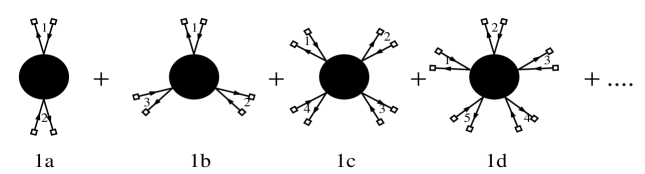
= \displaystyle= ∫ 𝒟 ψ 𝒟 ψ ¯ exp i { ∫ d 4 x ψ ¯ ( i ∂ / + J ) + ∑ n = 2 ∞ ∫ d 4 x 1 ⋯ d 4 x n i n n ! K α 1 β 1 ⋯ α n β n σ 1 ρ 1 ⋯ σ n ρ n ( x 1 , ⋯ , x n ) \displaystyle\int{\cal D}\psi{\cal D}\overline{\psi}\exp i{\{}{\int}d^{4}x\overline{\psi}(i\partial\!\!\!/+J)+\sum^{\infty}_{n=2}{\int}d^{4}x_{1}\cdots{d^{4}}x_{n}\frac{i^{n}}{n!}K^{\sigma_{1}\rho_{1}\cdots\sigma_{n}\rho_{n}}_{\alpha_{1}\beta_{1}\cdots\alpha_{n}\beta_{n}}(x_{1},\cdots,x_{n})
× [ ψ ¯ α 1 i 1 σ 1 ( x 1 ) ψ β 1 i 1 ρ 1 ( x 1 ) ] ⋯ [ ψ ¯ α n i n σ n ( x n ) ψ β n i n ρ n ( x n ) ] absent delimited-[] subscript superscript ¯ 𝜓 subscript 𝑖 1 subscript 𝜎 1 subscript 𝛼 1 subscript 𝑥 1 subscript superscript 𝜓 subscript 𝑖 1 subscript 𝜌 1 subscript 𝛽 1 subscript 𝑥 1 ⋯ delimited-[] subscript superscript ¯ 𝜓 subscript 𝑖 𝑛 subscript 𝜎 𝑛 subscript 𝛼 𝑛 subscript 𝑥 𝑛 subscript superscript 𝜓 subscript 𝑖 𝑛 subscript 𝜌 𝑛 subscript 𝛽 𝑛 subscript 𝑥 𝑛 \displaystyle\times[\overline{\psi}^{i_{1}\sigma_{1}}_{\alpha_{1}}(x_{1}){\psi}^{i_{1}\rho_{1}}_{\beta_{1}}(x_{1})]\cdots[\overline{\psi}^{i_{n}\sigma_{n}}_{\alpha_{n}}(x_{n}){\psi}^{i_{n}\rho_{n}}_{\beta_{n}}(x_{n})]
See Fig. 1.
Figure 1: Effective interactions caused by integrating out the gauge fields.
The blob with 2 n 2 𝑛 2n n 𝑛 n
The
K α 1 β 1 ⋯ α n β n σ 1 ρ 1 ⋯ σ n ρ n ( x 1 , ⋯ , x n ) subscript superscript 𝐾 subscript 𝜎 1 subscript 𝜌 1 ⋯ subscript 𝜎 𝑛 subscript 𝜌 𝑛 subscript 𝛼 1 subscript 𝛽 1 ⋯ subscript 𝛼 𝑛 subscript 𝛽 𝑛 subscript 𝑥 1 ⋯ subscript 𝑥 𝑛 K^{\sigma_{1}\rho_{1}\cdots\sigma_{n}\rho_{n}}_{\alpha_{1}\beta_{1}\cdots\alpha_{n}\beta_{n}}(x_{1},\cdots,x_{n})
K α 1 β 1 ⋯ α n β n σ 1 ρ 1 ⋯ σ n ρ n ( x 1 , ⋯ , x n ) subscript superscript 𝐾 subscript 𝜎 1 subscript 𝜌 1 ⋯ subscript 𝜎 𝑛 subscript 𝜌 𝑛 subscript 𝛼 1 subscript 𝛽 1 ⋯ subscript 𝛼 𝑛 subscript 𝛽 𝑛 subscript 𝑥 1 ⋯ subscript 𝑥 𝑛 \displaystyle K^{\sigma_{1}\rho_{1}\cdots\sigma_{n}\rho_{n}}_{\alpha_{1}\beta_{1}\cdots\alpha_{n}\beta_{n}}(x_{1},\cdots,x_{n}) = \displaystyle= g 2 n G μ 1 ⋯ μ n a 1 ⋯ a n ( x 1 , ⋯ , x n ) ( λ a 1 2 ) α 1 β 1 ( γ μ 1 ) σ 1 ρ 1 ⋯ ( λ a n n ) α n β n ( γ μ n ) σ n ρ n superscript 𝑔 2 𝑛 superscript subscript 𝐺 subscript 𝜇 1 ⋯ subscript 𝜇 𝑛 subscript 𝑎 1 ⋯ subscript 𝑎 𝑛 subscript 𝑥 1 ⋯ subscript 𝑥 𝑛 subscript subscript 𝜆 subscript 𝑎 1 2 subscript 𝛼 1 subscript 𝛽 1 subscript superscript 𝛾 subscript 𝜇 1 subscript 𝜎 1 subscript 𝜌 1 ⋯ subscript subscript 𝜆 subscript 𝑎 𝑛 𝑛 subscript 𝛼 𝑛 subscript 𝛽 𝑛 subscript superscript 𝛾 subscript 𝜇 𝑛 subscript 𝜎 𝑛 subscript 𝜌 𝑛 \displaystyle g^{2n}G_{\mu_{1}\cdots\mu_{n}}^{a_{1}\cdots a_{n}}(x_{1},\cdots,x_{n})(\frac{\lambda_{a_{1}}}{2})_{\alpha_{1}\beta_{1}}(\gamma^{\mu_{1}})_{\sigma_{1}\rho_{1}}\cdots(\frac{\lambda_{a_{n}}}{n})_{\alpha_{n}\beta_{n}}(\gamma^{\mu_{n}})_{\sigma_{n}\rho_{n}} (22)
+ δ n 2 g 1 2 G μ 1 μ 2 ( 1 ) ( x 1 , x 2 ) δ α 1 β 1 ( γ μ 1 ) σ 1 ρ 1 δ α 2 β 2 ( γ μ 2 ) σ 2 ρ 2 subscript 𝛿 𝑛 2 superscript subscript 𝑔 1 2 superscript subscript 𝐺 subscript 𝜇 1 subscript 𝜇 2 1 subscript 𝑥 1 subscript 𝑥 2 subscript 𝛿 subscript 𝛼 1 subscript 𝛽 1 subscript superscript 𝛾 subscript 𝜇 1 subscript 𝜎 1 subscript 𝜌 1 subscript 𝛿 subscript 𝛼 2 subscript 𝛽 2 subscript superscript 𝛾 subscript 𝜇 2 subscript 𝜎 2 subscript 𝜌 2 \displaystyle+\delta_{n2}g_{1}^{2}G_{\mu_{1}\mu_{2}}^{(1)}(x_{1},x_{2})\delta_{\alpha_{1}\beta_{1}}(\gamma^{\mu_{1}})_{\sigma_{1}\rho_{1}}\delta_{\alpha_{2}\beta_{2}}(\gamma^{\mu_{2}})_{\sigma_{2}\rho_{2}}
G μ 1 ⋯ μ n a 1 ⋯ a n ( x 1 , ⋯ , x n ) subscript superscript 𝐺 subscript 𝑎 1 ⋯ subscript 𝑎 𝑛 subscript 𝜇 1 ⋯ subscript 𝜇 𝑛 subscript 𝑥 1 ⋯ subscript 𝑥 𝑛 G^{a_{1}\cdots a_{n}}_{\mu_{1}\cdots\mu_{n}}(x_{1},\cdots,x_{n}) n 𝑛 n G μ ν ( 1 ) ( x , y ) subscript superscript 𝐺 1 𝜇 𝜈 𝑥 𝑦 G^{(1)}_{\mu\nu}(x,y) U ( 1 ) 𝑈 1 U(1)
We may rewrite the sum over n 𝑛 n 21
∑ n = 2 ∞ ∫ d 4 x 1 ⋯ d 4 x n ( i ) n n ! K α 1 β 1 ⋯ α n β n σ 1 ρ 1 ⋯ σ n ρ n ( x 1 , ⋯ , x n ) subscript superscript 𝑛 2 superscript 𝑑 4 subscript 𝑥 1 ⋯ superscript 𝑑 4 subscript 𝑥 𝑛 superscript 𝑖 𝑛 𝑛 subscript superscript 𝐾 subscript 𝜎 1 subscript 𝜌 1 ⋯ subscript 𝜎 𝑛 subscript 𝜌 𝑛 subscript 𝛼 1 subscript 𝛽 1 ⋯ subscript 𝛼 𝑛 subscript 𝛽 𝑛 subscript 𝑥 1 ⋯ subscript 𝑥 𝑛 \displaystyle\sum^{\infty}_{n=2}{\int}d^{4}x_{1}\cdots{d^{4}}x_{n}\frac{(i)^{n}}{n!}K^{\sigma_{1}\rho_{1}\cdots\sigma_{n}\rho_{n}}_{\alpha_{1}\beta_{1}\cdots\alpha_{n}\beta_{n}}(x_{1},\cdots,x_{n})
× [ ψ ¯ α 1 i 1 σ 1 ( x 1 ) ψ β n i n ρ n ( x n ) ] [ ψ ¯ α 2 i 2 σ 2 ( x 2 ) ψ β 1 i 1 ρ 1 ( x 1 ) ] ⋯ [ ψ ¯ α n i n σ n ( x n ) ψ β n − 1 i n − 1 ρ n − 1 ( x n − 1 ) ] absent delimited-[] subscript superscript ¯ 𝜓 subscript 𝑖 1 subscript 𝜎 1 subscript 𝛼 1 subscript 𝑥 1 subscript superscript 𝜓 subscript 𝑖 𝑛 subscript 𝜌 𝑛 subscript 𝛽 𝑛 subscript 𝑥 𝑛 delimited-[] subscript superscript ¯ 𝜓 subscript 𝑖 2 subscript 𝜎 2 subscript 𝛼 2 subscript 𝑥 2 subscript superscript 𝜓 subscript 𝑖 1 subscript 𝜌 1 subscript 𝛽 1 subscript 𝑥 1 ⋯ delimited-[] subscript superscript ¯ 𝜓 subscript 𝑖 𝑛 subscript 𝜎 𝑛 subscript 𝛼 𝑛 subscript 𝑥 𝑛 subscript superscript 𝜓 subscript 𝑖 𝑛 1 subscript 𝜌 𝑛 1 subscript 𝛽 𝑛 1 subscript 𝑥 𝑛 1 \displaystyle\times[\overline{\psi}^{i_{1}\sigma_{1}}_{\alpha_{1}}(x_{1}){\psi}^{i_{n}\rho_{n}}_{\beta_{n}}(x_{n})][\overline{\psi}^{i_{2}\sigma_{2}}_{\alpha_{2}}(x_{2}){\psi}^{i_{1}\rho_{1}}_{\beta_{1}}(x_{1})]\cdots[\overline{\psi}^{i_{n}\sigma_{n}}_{\alpha_{n}}(x_{n}){\psi}^{i_{n-1}\rho_{n-1}}_{\beta_{n-1}}(x_{n-1})]
= ∑ n = 1 ∞ ∫ d 4 x 1 ⋯ d 4 x 2 n ( i ) 2 n C 2 n n ( 2 n ) ! K α 1 β 1 ⋯ α 2 n β 2 n σ 1 ρ 1 ⋯ σ 2 n ρ 2 n ( x 1 , ⋯ , x 2 n ) absent subscript superscript 𝑛 1 superscript 𝑑 4 subscript 𝑥 1 ⋯ superscript 𝑑 4 subscript 𝑥 2 𝑛 superscript 𝑖 2 𝑛 superscript subscript 𝐶 2 𝑛 𝑛 2 𝑛 subscript superscript 𝐾 subscript 𝜎 1 subscript 𝜌 1 ⋯ subscript 𝜎 2 𝑛 subscript 𝜌 2 𝑛 subscript 𝛼 1 subscript 𝛽 1 ⋯ subscript 𝛼 2 𝑛 subscript 𝛽 2 𝑛 subscript 𝑥 1 ⋯ subscript 𝑥 2 𝑛 \displaystyle=\sum^{\infty}_{n=1}{\int}d^{4}x_{1}\cdots{d^{4}}x_{2n}\frac{(i)^{2n}C_{2n}^{n}}{(2n)!}K^{\sigma_{1}\rho_{1}\cdots\sigma_{2n}\rho_{2n}}_{\alpha_{1}\beta_{1}\cdots\alpha_{2n}\beta_{2n}}(x_{1},\cdots,x_{2n})
× [ ψ ¯ R , α 1 i 1 σ 1 ( x 1 ) ψ L , β 2 n i 2 n ρ 2 n ( x 2 n ) ] [ ψ ¯ L , α 2 i 2 σ 2 ( x 2 ) ψ R , β 1 i 1 ρ 1 ( x 1 ) ] ⋯ absent delimited-[] subscript superscript ¯ 𝜓 subscript 𝑖 1 subscript 𝜎 1 𝑅 subscript 𝛼 1
subscript 𝑥 1 subscript superscript 𝜓 subscript 𝑖 2 𝑛 subscript 𝜌 2 𝑛 𝐿 subscript 𝛽 2 𝑛
subscript 𝑥 2 𝑛 delimited-[] subscript superscript ¯ 𝜓 subscript 𝑖 2 subscript 𝜎 2 𝐿 subscript 𝛼 2
subscript 𝑥 2 subscript superscript 𝜓 subscript 𝑖 1 subscript 𝜌 1 𝑅 subscript 𝛽 1
subscript 𝑥 1 ⋯ \displaystyle\times[\overline{\psi}^{i_{1}\sigma_{1}}_{R,\alpha_{1}}(x_{1}){\psi}^{i_{2n}\rho_{2n}}_{L,\beta_{2n}}(x_{2n})][\overline{\psi}^{i_{2}\sigma_{2}}_{L,\alpha_{2}}(x_{2}){\psi}^{i_{1}\rho_{1}}_{R,\beta_{1}}(x_{1})]\cdots
⋯ [ ψ ¯ R , α 2 n − 1 i 2 n − 1 σ 2 n − 1 ( x 2 n − 1 ) ψ L , β 2 n − 2 i 2 n − 2 ρ 2 n − 2 ( x 2 n − 2 ) ] [ ψ ¯ L , α 2 n i 2 n σ 2 n ( x 2 n ) ψ R , β 2 n − 1 i 2 n − 1 ρ 2 n − 1 ( x 2 n − 1 ) ] ⋯ delimited-[] subscript superscript ¯ 𝜓 subscript 𝑖 2 𝑛 1 subscript 𝜎 2 𝑛 1 𝑅 subscript 𝛼 2 𝑛 1
subscript 𝑥 2 𝑛 1 subscript superscript 𝜓 subscript 𝑖 2 𝑛 2 subscript 𝜌 2 𝑛 2 𝐿 subscript 𝛽 2 𝑛 2
subscript 𝑥 2 𝑛 2 delimited-[] subscript superscript ¯ 𝜓 subscript 𝑖 2 𝑛 subscript 𝜎 2 𝑛 𝐿 subscript 𝛼 2 𝑛
subscript 𝑥 2 𝑛 subscript superscript 𝜓 subscript 𝑖 2 𝑛 1 subscript 𝜌 2 𝑛 1 𝑅 subscript 𝛽 2 𝑛 1
subscript 𝑥 2 𝑛 1 \displaystyle\cdots[\overline{\psi}^{i_{2n-1}\sigma_{2n-1}}_{R,\alpha_{2n-1}}(x_{2n-1}){\psi}^{i_{2n-2}\rho_{2n-2}}_{L,\beta_{2n-2}}(x_{2n-2})][\overline{\psi}^{i_{2n}\sigma_{2n}}_{L,\alpha_{2n}}(x_{2n}){\psi}^{i_{2n-1}\rho_{2n-1}}_{R,\beta_{2n-1}}(x_{2n-1})]
+ ∑ n = 2 ∞ ∫ d 4 x 1 ⋯ d 4 x n ( i ) n n ! K ¯ α 1 β 1 ⋯ α n β n σ 1 ρ 1 ⋯ σ n ρ n ( x 1 , ⋯ , x n ) subscript superscript 𝑛 2 superscript 𝑑 4 subscript 𝑥 1 ⋯ superscript 𝑑 4 subscript 𝑥 𝑛 superscript 𝑖 𝑛 𝑛 subscript superscript ¯ 𝐾 subscript 𝜎 1 subscript 𝜌 1 ⋯ subscript 𝜎 𝑛 subscript 𝜌 𝑛 subscript 𝛼 1 subscript 𝛽 1 ⋯ subscript 𝛼 𝑛 subscript 𝛽 𝑛 subscript 𝑥 1 ⋯ subscript 𝑥 𝑛 \displaystyle+\sum^{\infty}_{n=2}{\int}d^{4}x_{1}\cdots{d^{4}}x_{n}\frac{(i)^{n}}{n!}\bar{K}^{\sigma_{1}\rho_{1}\cdots\sigma_{n}\rho_{n}}_{\alpha_{1}\beta_{1}\cdots\alpha_{n}\beta_{n}}(x_{1},\cdots,x_{n})
× [ ψ ¯ α 1 i 1 σ 1 ( x 1 ) ψ β 1 i 1 ρ 1 ( x 1 ) ] [ ψ ¯ α 2 i 2 σ 2 ( x 2 ) ψ β 2 i 2 ρ 2 ( x 2 ) ] ⋯ [ ψ ¯ α n i n σ n ( x n ) ψ β n i n ρ n ( x n ) ] absent delimited-[] subscript superscript ¯ 𝜓 subscript 𝑖 1 subscript 𝜎 1 subscript 𝛼 1 subscript 𝑥 1 subscript superscript 𝜓 subscript 𝑖 1 subscript 𝜌 1 subscript 𝛽 1 subscript 𝑥 1 delimited-[] subscript superscript ¯ 𝜓 subscript 𝑖 2 subscript 𝜎 2 subscript 𝛼 2 subscript 𝑥 2 subscript superscript 𝜓 subscript 𝑖 2 subscript 𝜌 2 subscript 𝛽 2 subscript 𝑥 2 ⋯ delimited-[] subscript superscript ¯ 𝜓 subscript 𝑖 𝑛 subscript 𝜎 𝑛 subscript 𝛼 𝑛 subscript 𝑥 𝑛 subscript superscript 𝜓 subscript 𝑖 𝑛 subscript 𝜌 𝑛 subscript 𝛽 𝑛 subscript 𝑥 𝑛 \displaystyle\times[\overline{\psi}^{i_{1}\sigma_{1}}_{\alpha_{1}}(x_{1}){\psi}^{i_{1}\rho_{1}}_{\beta_{1}}(x_{1})][\overline{\psi}^{i_{2}\sigma_{2}}_{\alpha_{2}}(x_{2}){\psi}^{i_{2}\rho_{2}}_{\beta_{2}}(x_{2})]\cdots[\overline{\psi}^{i_{n}\sigma_{n}}_{\alpha_{n}}(x_{n}){\psi}^{i_{n}\rho_{n}}_{\beta_{n}}(x_{n})] (23)
where K ¯ ¯ 𝐾 \bar{K} C n m = n ! m ! ( n − m ) ! subscript superscript 𝐶 𝑚 𝑛 𝑛 𝑚 𝑛 𝑚 C^{m}_{n}=\frac{n!}{m!(n-m)!}
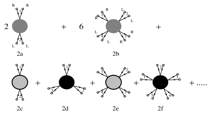
Figure 2: The chirality (denoted by L and R) changing part is explicitly
separated out, such that diagram 1a (from Fig. 1) is separated
into diagram 2a (the chirality changing part) and diagram 2c, and diagram
1c is similarly separated into diagrams 2b and 2e.
Inserting this back into the
generating functional and introducing auxiliary fields gives the following.
Z [ J ] 𝑍 delimited-[] 𝐽 \displaystyle Z[J] = \displaystyle= e i W [ J ] superscript 𝑒 𝑖 𝑊 delimited-[] 𝐽 \displaystyle e^{iW[J]} (24)
= \displaystyle= ∫ 𝒟 S R 𝒟 S L 𝒟 F ¯ 𝒟 F 𝒟 B ¯ 𝒟 B 𝒟 ψ 𝒟 ψ ¯ δ ( S R , α β i σ j ρ ( x , y ) − ψ ¯ L , α i σ ( x ) ψ R , β j ρ ( y ) ) 𝒟 subscript 𝑆 𝑅 𝒟 subscript 𝑆 𝐿 𝒟 ¯ 𝐹 𝒟 𝐹 𝒟 ¯ 𝐵 𝒟 𝐵 𝒟 𝜓 𝒟 ¯ 𝜓 𝛿 subscript superscript 𝑆 𝑖 𝜎 𝑗 𝜌 𝑅 𝛼 𝛽
𝑥 𝑦 subscript superscript ¯ 𝜓 𝑖 𝜎 𝐿 𝛼
𝑥 subscript superscript 𝜓 𝑗 𝜌 𝑅 𝛽
𝑦 \displaystyle\int{\cal D}S_{R}{\cal D}S_{L}{\cal D}\overline{F}{\cal D}F{\cal D}\overline{B}{\cal D}B{\cal D}\psi{\cal D}\overline{\psi}\delta\bigg{(}S^{i\sigma j\rho}_{R,\alpha\beta}(x,y)-\overline{\psi}^{i\sigma}_{L,\alpha}(x){\psi}^{j\rho}_{R,\beta}(y)\bigg{)}
× δ ( S L , α β i σ j ρ ( x , y ) − ψ ¯ R , α i σ ( x ) ψ L , β j ρ ( y ) ) δ ( F ¯ α β i σ j ρ ( x , y ) − ψ ¯ α i σ ( x ) ψ ¯ β j ρ ( y ) ) absent 𝛿 subscript superscript 𝑆 𝑖 𝜎 𝑗 𝜌 𝐿 𝛼 𝛽
𝑥 𝑦 subscript superscript ¯ 𝜓 𝑖 𝜎 𝑅 𝛼
𝑥 subscript superscript 𝜓 𝑗 𝜌 𝐿 𝛽
𝑦 𝛿 superscript subscript ¯ 𝐹 𝛼 𝛽 𝑖 𝜎 𝑗 𝜌 𝑥 𝑦 subscript superscript ¯ 𝜓 𝑖 𝜎 𝛼 𝑥 subscript superscript ¯ 𝜓 𝑗 𝜌 𝛽 𝑦 \displaystyle\times\delta\bigg{(}S^{i\sigma j\rho}_{L,\alpha\beta}(x,y)-\overline{\psi}^{i\sigma}_{R,\alpha}(x){\psi}^{j\rho}_{L,\beta}(y)\bigg{)}\delta\bigg{(}\overline{F}_{\alpha\beta}^{i\sigma j\rho}(x,y)-\overline{\psi}^{i\sigma}_{\alpha}(x)\overline{\psi}^{j\rho}_{\beta}(y)\bigg{)}
× δ ( F α β i σ j ρ ( x , y ) − ψ α i σ ( x ) ψ β j ρ ( y ) ) δ ( B ¯ α 1 α 2 α 3 i 1 σ 1 i 2 σ 2 i 3 σ 3 ( x 1 , x 2 , x 3 ) − ψ ¯ α 1 i 1 σ 1 ( x 1 ) ψ ¯ α 2 i 2 σ 2 ( x 2 ) ψ ¯ α 3 i 3 σ 3 ( x 3 ) ) absent 𝛿 superscript subscript 𝐹 𝛼 𝛽 𝑖 𝜎 𝑗 𝜌 𝑥 𝑦 subscript superscript 𝜓 𝑖 𝜎 𝛼 𝑥 subscript superscript 𝜓 𝑗 𝜌 𝛽 𝑦 𝛿 superscript subscript ¯ 𝐵 subscript 𝛼 1 subscript 𝛼 2 subscript 𝛼 3 subscript 𝑖 1 subscript 𝜎 1 subscript 𝑖 2 subscript 𝜎 2 subscript 𝑖 3 subscript 𝜎 3 subscript 𝑥 1 subscript 𝑥 2 subscript 𝑥 3 subscript superscript ¯ 𝜓 subscript 𝑖 1 subscript 𝜎 1 subscript 𝛼 1 subscript 𝑥 1 subscript superscript ¯ 𝜓 subscript 𝑖 2 subscript 𝜎 2 subscript 𝛼 2 subscript 𝑥 2 subscript superscript ¯ 𝜓 subscript 𝑖 3 subscript 𝜎 3 subscript 𝛼 3 subscript 𝑥 3 \displaystyle\times\delta\bigg{(}F_{\alpha\beta}^{i\sigma j\rho}(x,y)-\psi^{i\sigma}_{\alpha}(x)\psi^{j\rho}_{\beta}(y)\bigg{)}\delta\bigg{(}\overline{B}_{\alpha_{1}\alpha_{2}\alpha_{3}}^{i_{1}\sigma_{1}i_{2}\sigma_{2}i_{3}\sigma_{3}}(x_{1},x_{2},x_{3})-\overline{\psi}^{i_{1}\sigma_{1}}_{\alpha_{1}}(x_{1})\overline{\psi}^{i_{2}\sigma_{2}}_{\alpha_{2}}(x_{2})\overline{\psi}^{i_{3}\sigma_{3}}_{\alpha_{3}}(x_{3})\bigg{)}
× δ ( B α 1 α 2 α 3 i 1 σ 1 i 2 σ 2 i 3 σ 3 ( x 1 , x 2 , x 3 ) − ψ α 1 i 1 σ 1 ( x 1 ) ψ α 2 i 2 σ 2 ( x 2 ) ψ α 3 i 3 σ 3 ( x 3 ) ) exp i { ∫ d 4 x ψ ¯ ( i ∂ / + J ) ψ \displaystyle\times\delta\bigg{(}B_{\alpha_{1}\alpha_{2}\alpha_{3}}^{i_{1}\sigma_{1}i_{2}\sigma_{2}i_{3}\sigma_{3}}(x_{1},x_{2},x_{3})-\psi^{i_{1}\sigma_{1}}_{\alpha_{1}}(x_{1})\psi^{i_{2}\sigma_{2}}_{\alpha_{2}}(x_{2})\psi^{i_{3}\sigma_{3}}_{\alpha_{3}}(x_{3})\bigg{)}\exp i{\bigg{\{}}{\int}d^{4}x\overline{\psi}(i\partial\!\!\!/+J){\psi}
+ ∑ n = 1 ∞ ∫ d 4 x 1 ⋯ d 4 x 2 n ( i ) 2 n C 2 n n ( 2 n ) ! K α 1 β 1 ⋯ α 2 n β 2 n σ 1 ρ 1 ⋯ σ 2 n ρ 2 n ( x 1 , ⋯ , x 2 n ) subscript superscript 𝑛 1 superscript 𝑑 4 subscript 𝑥 1 ⋯ superscript 𝑑 4 subscript 𝑥 2 𝑛 superscript 𝑖 2 𝑛 superscript subscript 𝐶 2 𝑛 𝑛 2 𝑛 subscript superscript 𝐾 subscript 𝜎 1 subscript 𝜌 1 ⋯ subscript 𝜎 2 𝑛 subscript 𝜌 2 𝑛 subscript 𝛼 1 subscript 𝛽 1 ⋯ subscript 𝛼 2 𝑛 subscript 𝛽 2 𝑛 subscript 𝑥 1 ⋯ subscript 𝑥 2 𝑛 \displaystyle+\sum^{\infty}_{n=1}{\int}d^{4}x_{1}\cdots{d^{4}}x_{2n}\frac{(i)^{2n}C_{2n}^{n}}{(2n)!}K^{\sigma_{1}\rho_{1}\cdots\sigma_{2n}\rho_{2n}}_{\alpha_{1}\beta_{1}\cdots\alpha_{2n}\beta_{2n}}(x_{1},\cdots,x_{2n})
× S L , α 1 β 2 n i 1 σ 1 i 2 n ρ 2 n ( x 1 , x 2 n ) S R , α 2 β 1 i 2 σ 2 i 1 ρ 1 ( x 2 , x 1 ) ⋯ absent subscript superscript 𝑆 subscript 𝑖 1 subscript 𝜎 1 subscript 𝑖 2 𝑛 subscript 𝜌 2 𝑛 𝐿 subscript 𝛼 1 subscript 𝛽 2 𝑛
subscript 𝑥 1 subscript 𝑥 2 𝑛 subscript superscript 𝑆 subscript 𝑖 2 subscript 𝜎 2 subscript 𝑖 1 subscript 𝜌 1 𝑅 subscript 𝛼 2 subscript 𝛽 1
subscript 𝑥 2 subscript 𝑥 1 ⋯ \displaystyle\times S^{i_{1}\sigma_{1}i_{2n}\rho_{2n}}_{L,\alpha_{1}\beta_{2n}}(x_{1},x_{2n})S^{i_{2}\sigma_{2}i_{1}\rho_{1}}_{R,\alpha_{2}\beta_{1}}(x_{2},x_{1})\cdots
⋯ S L , α 2 n − 1 β 2 n − 2 i 2 n − 1 σ 2 n − 1 i 2 n − 2 ρ 2 n − 2 ( x 2 n − 1 , x 2 n − 2 ) S R , α 2 n β 2 n − 1 i 2 n σ 2 n i 2 n − 1 ρ 2 n − 1 ( x 2 n , x 2 n − 1 ) ⋯ subscript superscript 𝑆 subscript 𝑖 2 𝑛 1 subscript 𝜎 2 𝑛 1 subscript 𝑖 2 𝑛 2 subscript 𝜌 2 𝑛 2 𝐿 subscript 𝛼 2 𝑛 1 subscript 𝛽 2 𝑛 2
subscript 𝑥 2 𝑛 1 subscript 𝑥 2 𝑛 2 subscript superscript 𝑆 subscript 𝑖 2 𝑛 subscript 𝜎 2 𝑛 subscript 𝑖 2 𝑛 1 subscript 𝜌 2 𝑛 1 𝑅 subscript 𝛼 2 𝑛 subscript 𝛽 2 𝑛 1
subscript 𝑥 2 𝑛 subscript 𝑥 2 𝑛 1 \displaystyle\cdots S^{i_{2n-1}\sigma_{2n-1}i_{2n-2}\rho_{2n-2}}_{L,\alpha_{2n-1}\beta_{2n-2}}(x_{2n-1},x_{2n-2})S^{i_{2n}\sigma_{2n}i_{2n-1}\rho_{2n-1}}_{R,\alpha_{2n}\beta_{2n-1}}(x_{2n},x_{2n-1})
− ∑ n = 1 ∞ ∫ d 4 x 1 ⋯ d 4 x 2 n ( i ) 2 n ( 2 n ) ! K ¯ α 1 β 1 ⋯ α 2 n β 2 n σ 1 ρ 1 ⋯ σ 2 n ρ 2 n ( x 1 , ⋯ , x 2 n ) subscript superscript 𝑛 1 superscript 𝑑 4 subscript 𝑥 1 ⋯ superscript 𝑑 4 subscript 𝑥 2 𝑛 superscript 𝑖 2 𝑛 2 𝑛 subscript superscript ¯ 𝐾 subscript 𝜎 1 subscript 𝜌 1 ⋯ subscript 𝜎 2 𝑛 subscript 𝜌 2 𝑛 subscript 𝛼 1 subscript 𝛽 1 ⋯ subscript 𝛼 2 𝑛 subscript 𝛽 2 𝑛 subscript 𝑥 1 ⋯ subscript 𝑥 2 𝑛 \displaystyle-\sum^{\infty}_{n=1}{\int}d^{4}x_{1}\cdots{d^{4}}x_{2n}\frac{(i)^{2n}}{(2n)!}\bar{K}^{\sigma_{1}\rho_{1}\cdots\sigma_{2n}\rho_{2n}}_{\alpha_{1}\beta_{1}\cdots\alpha_{2n}\beta_{2n}}(x_{1},\cdots,x_{2n})
× F ¯ α 2 n α 1 i 2 n σ 2 n i 1 σ 1 ( x 2 n , x 1 ) ⋯ F ¯ α 2 n − 2 α 2 n − 1 i 2 n − 2 σ 2 n − 2 i 2 n − 1 α 2 n − 1 ( x 2 n − 2 , x 2 n − 1 ) absent subscript superscript ¯ 𝐹 subscript 𝑖 2 𝑛 subscript 𝜎 2 𝑛 subscript 𝑖 1 subscript 𝜎 1 subscript 𝛼 2 𝑛 subscript 𝛼 1 subscript 𝑥 2 𝑛 subscript 𝑥 1 ⋯ subscript superscript ¯ 𝐹 subscript 𝑖 2 𝑛 2 subscript 𝜎 2 𝑛 2 subscript 𝑖 2 𝑛 1 subscript 𝛼 2 𝑛 1 subscript 𝛼 2 𝑛 2 subscript 𝛼 2 𝑛 1 subscript 𝑥 2 𝑛 2 subscript 𝑥 2 𝑛 1 \displaystyle\times\overline{F}^{i_{2n}\sigma_{2n}i_{1}\sigma_{1}}_{\alpha_{2n}\alpha_{1}}(x_{2n},x_{1})\cdots\overline{F}^{i_{2n-2}\sigma_{2n-2}i_{2n-1}\alpha_{2n-1}}_{\alpha_{2n-2}\alpha_{2n-1}}(x_{2n-2},x_{2n-1})
× F β 1 β 2 i 1 ρ 1 i 2 ρ 2 ( x 1 , x 2 ) ⋯ F β 2 n − 1 β 2 n i 2 n − 1 ρ 2 n − 1 i 2 n ρ 2 n ( x 2 n − 1 , x 2 n ) absent subscript superscript 𝐹 subscript 𝑖 1 subscript 𝜌 1 subscript 𝑖 2 subscript 𝜌 2 subscript 𝛽 1 subscript 𝛽 2 subscript 𝑥 1 subscript 𝑥 2 ⋯ subscript superscript 𝐹 subscript 𝑖 2 𝑛 1 subscript 𝜌 2 𝑛 1 subscript 𝑖 2 𝑛 subscript 𝜌 2 𝑛 subscript 𝛽 2 𝑛 1 subscript 𝛽 2 𝑛 subscript 𝑥 2 𝑛 1 subscript 𝑥 2 𝑛 \displaystyle\times F^{i_{1}\rho_{1}i_{2}\rho_{2}}_{\beta_{1}\beta_{2}}(x_{1},x_{2})\cdots F^{i_{2n-1}\rho_{2n-1}i_{2n}\rho_{2n}}_{\beta_{2n-1}\beta_{2n}}(x_{2n-1},x_{2n})
− ∑ n = 1 ∞ ∫ d 4 x 1 ⋯ d 4 x 2 n + 1 ( i ) 2 n + 1 ( 2 n + 1 ) ! K ¯ α 1 β 1 ⋯ α 2 n + 1 β 2 n + 1 σ 1 ρ 1 ⋯ σ 2 n + 1 ρ 2 n + 1 ( x 1 , ⋯ , x 2 n + 1 ) subscript superscript 𝑛 1 superscript 𝑑 4 subscript 𝑥 1 ⋯ superscript 𝑑 4 subscript 𝑥 2 𝑛 1 superscript 𝑖 2 𝑛 1 2 𝑛 1 subscript superscript ¯ 𝐾 subscript 𝜎 1 subscript 𝜌 1 ⋯ subscript 𝜎 2 𝑛 1 subscript 𝜌 2 𝑛 1 subscript 𝛼 1 subscript 𝛽 1 ⋯ subscript 𝛼 2 𝑛 1 subscript 𝛽 2 𝑛 1 subscript 𝑥 1 ⋯ subscript 𝑥 2 𝑛 1 \displaystyle-\sum^{\infty}_{n=1}{\int}d^{4}x_{1}\cdots{d^{4}}x_{2n+1}\frac{(i)^{2n+1}}{(2n+1)!}\bar{K}^{\sigma_{1}\rho_{1}\cdots\sigma_{2n+1}\rho_{2n+1}}_{\alpha_{1}\beta_{1}\cdots\alpha_{2n+1}\beta_{2n+1}}(x_{1},\cdots,x_{2n+1})
× B ¯ α 1 α 2 α 3 i 1 σ 1 i 2 σ 2 i 3 σ 3 ( x 1 , x 2 , x 3 ) F ¯ α 4 α 5 i 4 σ 4 i 5 σ 5 ( x 4 , x 5 ) ⋯ F ¯ α 2 n α 2 n + 1 i 2 n σ 2 n i 2 n + 1 σ 2 n + 1 ( x 2 n , x 2 n + 1 ) absent subscript superscript ¯ 𝐵 subscript 𝑖 1 subscript 𝜎 1 subscript 𝑖 2 subscript 𝜎 2 subscript 𝑖 3 subscript 𝜎 3 subscript 𝛼 1 subscript 𝛼 2 subscript 𝛼 3 subscript 𝑥 1 subscript 𝑥 2 subscript 𝑥 3 subscript superscript ¯ 𝐹 subscript 𝑖 4 subscript 𝜎 4 subscript 𝑖 5 subscript 𝜎 5 subscript 𝛼 4 subscript 𝛼 5 subscript 𝑥 4 subscript 𝑥 5 ⋯ subscript superscript ¯ 𝐹 subscript 𝑖 2 𝑛 subscript 𝜎 2 𝑛 subscript 𝑖 2 𝑛 1 subscript 𝜎 2 𝑛 1 subscript 𝛼 2 𝑛 subscript 𝛼 2 𝑛 1 subscript 𝑥 2 𝑛 subscript 𝑥 2 𝑛 1 \displaystyle\times\overline{B}^{i_{1}\sigma_{1}i_{2}\sigma_{2}i_{3}\sigma_{3}}_{\alpha_{1}\alpha_{2}\alpha_{3}}(x_{1},x_{2},x_{3})\overline{F}^{i_{4}\sigma_{4}i_{5}\sigma_{5}}_{\alpha_{4}\alpha_{5}}(x_{4},x_{5})\cdots\overline{F}^{i_{2n}\sigma_{2n}i_{2n+1}\sigma_{2n+1}}_{\alpha_{2n}\alpha_{2n+1}}(x_{2n},x_{2n+1})
× B α 1 α 2 α 3 i 1 ρ 1 i 2 ρ 2 i 3 ρ 3 ( x 1 , x 2 , x 3 ) F α 4 α 5 i 4 ρ 4 i 5 ρ 5 ( x 4 , x 5 ) ⋯ F α 2 n α 2 n + 1 i 2 n ρ 2 n i 2 n + 1 ρ 2 n + 1 ( x 2 n , x 2 n + 1 ) } \displaystyle\times B^{i_{1}\rho_{1}i_{2}\rho_{2}i_{3}\rho_{3}}_{\alpha_{1}\alpha_{2}\alpha_{3}}(x_{1},x_{2},x_{3})F^{i_{4}\rho_{4}i_{5}\rho_{5}}_{\alpha_{4}\alpha_{5}}(x_{4},x_{5})\cdots F^{i_{2n}\rho_{2n}i_{2n+1}\rho_{2n+1}}_{\alpha_{2n}\alpha_{2n+1}}(x_{2n},x_{2n+1})\bigg{\}}
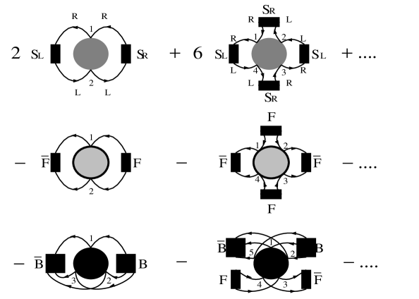
See Fig. 3.
Figure 3: The fermion fields in diagrams 2a, 2c, and 2d in Fig. 2 are
combined with the appropriate composite auxiliary fields.
We can remove the delta functions by instead including
the following terms in the exponential and integrating over the
additional auxiliary fields, χ L subscript 𝜒 𝐿 \chi_{L} χ R subscript 𝜒 𝑅 \chi_{R} U 𝑈 U U ¯ ¯ 𝑈 \overline{U} V 𝑉 V V ¯ ¯ 𝑉 \overline{V}
i ∫ d 4 x d 4 y [ ( S R , α β i σ j ρ ( x , y ) − ψ ¯ L , α i σ ( x ) ψ R , β j ρ ( y ) ) χ R , α β i σ j ρ ( x , y ) \displaystyle i\int d^{4}xd^{4}y\bigg{[}\bigg{(}S^{i\sigma j\rho}_{R,\alpha\beta}(x,y)-\overline{\psi}^{i\sigma}_{L,\alpha}(x){\psi}^{j\rho}_{R,\beta}(y)\bigg{)}\chi^{i\sigma j\rho}_{R,\alpha\beta}(x,y)
+ ( S L , α β i σ j ρ ( x , y ) − ψ ¯ R , α i σ ( x ) ψ L , α j ρ ( y ) ) χ L , α β i σ j ρ ( x , y ) + ( F ¯ α β i σ j ρ ( x , y ) − ψ ¯ α i σ ( x ) ψ ¯ β j ρ ( y ) ) U α β i σ j ρ ( x , y ) subscript superscript 𝑆 𝑖 𝜎 𝑗 𝜌 𝐿 𝛼 𝛽
𝑥 𝑦 subscript superscript ¯ 𝜓 𝑖 𝜎 𝑅 𝛼
𝑥 subscript superscript 𝜓 𝑗 𝜌 𝐿 𝛼
𝑦 subscript superscript 𝜒 𝑖 𝜎 𝑗 𝜌 𝐿 𝛼 𝛽
𝑥 𝑦 superscript subscript ¯ 𝐹 𝛼 𝛽 𝑖 𝜎 𝑗 𝜌 𝑥 𝑦 subscript superscript ¯ 𝜓 𝑖 𝜎 𝛼 𝑥 subscript superscript ¯ 𝜓 𝑗 𝜌 𝛽 𝑦 superscript subscript 𝑈 𝛼 𝛽 𝑖 𝜎 𝑗 𝜌 𝑥 𝑦 \displaystyle+\bigg{(}S^{i\sigma j\rho}_{L,\alpha\beta}(x,y)-\overline{\psi}^{i\sigma}_{R,\alpha}(x){\psi}^{j\rho}_{L,\alpha}(y)\bigg{)}\chi^{i\sigma j\rho}_{L,\alpha\beta}(x,y)+\bigg{(}\overline{F}_{\alpha\beta}^{i\sigma j\rho}(x,y)-\overline{\psi}^{i\sigma}_{\alpha}(x)\overline{\psi}^{j\rho}_{\beta}(y)\bigg{)}U_{\alpha\beta}^{i\sigma j\rho}(x,y)
+ U ¯ α β i σ j ρ ( x , y ) ( F α β i σ j ρ ( x , y ) − ψ α i σ ( x ) ψ β j ρ ( y ) ) ] \displaystyle+\overline{U}_{\alpha\beta}^{i\sigma j\rho}(x,y)\bigg{(}F_{\alpha\beta}^{i\sigma j\rho}(x,y)-\psi^{i\sigma}_{\alpha}(x)\psi^{j\rho}_{\beta}(y)\bigg{)}\bigg{]}
+ i ∫ d 4 x 1 d 4 x 2 d 4 x 3 [ ( B ¯ α 1 α 2 α 3 i 1 σ 1 i 2 σ 2 i 3 σ 3 ( x 1 , x 2 , x 3 ) − ψ ¯ α 1 i 1 σ 1 ( x 1 ) ψ ¯ α 2 i 2 σ 2 ( x 2 ) ψ ¯ α 3 i 3 σ 3 ( x 3 ) ) V α 1 α 2 α 3 i 1 σ 1 i 2 σ 2 i 3 σ 3 ( x 1 , x 2 , x 3 ) \displaystyle+i\int d^{4}x_{1}d^{4}x_{2}d^{4}x_{3}\bigg{[}\bigg{(}\overline{B}_{\alpha_{1}\alpha_{2}\alpha_{3}}^{i_{1}\sigma_{1}i_{2}\sigma_{2}i_{3}\sigma_{3}}(x_{1},x_{2},x_{3})-\overline{\psi}^{i_{1}\sigma_{1}}_{\alpha_{1}}(x_{1})\overline{\psi}^{i_{2}\sigma_{2}}_{\alpha_{2}}(x_{2})\overline{\psi}^{i_{3}\sigma_{3}}_{\alpha_{3}}(x_{3})\bigg{)}V_{\alpha_{1}\alpha_{2}\alpha_{3}}^{i_{1}\sigma_{1}i_{2}\sigma_{2}i_{3}\sigma_{3}}(x_{1},x_{2},x_{3})
+ V ¯ α 1 α 2 α 3 i 1 σ 1 i 2 σ 2 i 3 σ 3 ( x 1 , x 2 , x 3 ) ( B α 1 α 2 α 3 i 1 σ 1 i 2 σ 2 i 3 σ 3 ( x 1 , x 2 , x 3 ) − ψ α 1 i 1 σ 1 ( x 1 ) ψ α 2 i 2 σ 2 ( x 2 ) ψ α 3 i 3 σ 3 ( x 3 ) ) ] \displaystyle+\overline{V}_{\alpha_{1}\alpha_{2}\alpha_{3}}^{i_{1}\sigma_{1}i_{2}\sigma_{2}i_{3}\sigma_{3}}(x_{1},x_{2},x_{3})\bigg{(}B_{\alpha_{1}\alpha_{2}\alpha_{3}}^{i_{1}\sigma_{1}i_{2}\sigma_{2}i_{3}\sigma_{3}}(x_{1},x_{2},x_{3})-\psi^{i_{1}\sigma_{1}}_{\alpha_{1}}(x_{1})\psi^{i_{2}\sigma_{2}}_{\alpha_{2}}(x_{2})\psi^{i_{3}\sigma_{3}}_{\alpha_{3}}(x_{3})\bigg{)}\bigg{]}
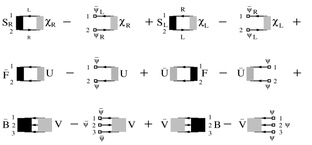
See Fig. 4.
Figure 4: These new terms are caused by realizing the constraints
among the fermion fields and the composite auxiliary fields.
We may write the result as follows.
e i W [ J ] superscript 𝑒 𝑖 𝑊 delimited-[] 𝐽 \displaystyle e^{iW[J]} = \displaystyle= ∫ 𝒟 S R 𝒟 S L 𝒟 χ R 𝒟 χ L 𝒟 F ¯ 𝒟 F 𝒟 U ¯ 𝒟 U 𝒟 B ¯ 𝒟 B 𝒟 V ¯ 𝒟 V exp i { D [ χ R , χ L , U ¯ , U , V ¯ , V , J ] \displaystyle\int{\cal D}S_{R}{\cal D}S_{L}{\cal D}\chi_{R}{\cal D}\chi_{L}{\cal D}\overline{F}{\cal D}F{\cal D}\overline{U}{\cal D}U{\cal D}\overline{B}{\cal D}B{\cal D}\overline{V}{\cal D}V{\rm exp}i\bigg{\{}D[\chi_{R},\chi_{L},\overline{U},U,\overline{V},V,J] (25)
+ ∫ d 4 x d 4 y [ [ S R , α β i σ j ρ ( x , y ) χ R , α β i σ j ρ ( x , y ) + S L , α β i σ j ρ ( x , y ) χ L , α β i σ j ρ ( x , y ) ] + F ¯ α β i σ j ρ ( x , y ) U α β i σ j ρ ( x , y ) \displaystyle+\int d^{4}xd^{4}y\bigg{[}[S^{i\sigma j\rho}_{R,\alpha\beta}(x,y)\chi^{i\sigma j\rho}_{R,\alpha\beta}(x,y)+S^{i\sigma j\rho}_{L,\alpha\beta}(x,y)\chi^{i\sigma j\rho}_{L,\alpha\beta}(x,y)]+\overline{F}_{\alpha\beta}^{i\sigma j\rho}(x,y)U_{\alpha\beta}^{i\sigma j\rho}(x,y)
+ U ¯ α β i σ j ρ ( x , y ) F α β i σ j ρ ( x , y ) ] + ∫ d 4 x 1 d 4 x 2 d 4 x 3 [ B ¯ α 1 α 2 α 3 i 1 σ 1 i 2 σ 2 i 3 σ 3 ( x 1 , x 2 , x 3 ) V α 1 α 2 α 3 i 1 σ 1 i 2 σ 2 i 3 σ 3 ( x 1 , x 2 , x 3 ) \displaystyle+\overline{U}_{\alpha\beta}^{i\sigma j\rho}(x,y)F_{\alpha\beta}^{i\sigma j\rho}(x,y)\bigg{]}+\int d^{4}x_{1}d^{4}x_{2}d^{4}x_{3}[\overline{B}_{\alpha_{1}\alpha_{2}\alpha_{3}}^{i_{1}\sigma_{1}i_{2}\sigma_{2}i_{3}\sigma_{3}}(x_{1},x_{2},x_{3})V_{\alpha_{1}\alpha_{2}\alpha_{3}}^{i_{1}\sigma_{1}i_{2}\sigma_{2}i_{3}\sigma_{3}}(x_{1},x_{2},x_{3})
+ V ¯ α 1 α 2 α 3 i 1 σ 1 i 2 σ 2 i 3 σ 3 ( x 1 , x 2 , x 3 ) B α 1 α 2 α 3 i 1 σ 1 i 2 σ 2 i 3 σ 3 ( x 1 , x 2 , x 3 ) ] \displaystyle+\overline{V}_{\alpha_{1}\alpha_{2}\alpha_{3}}^{i_{1}\sigma_{1}i_{2}\sigma_{2}i_{3}\sigma_{3}}(x_{1},x_{2},x_{3})B_{\alpha_{1}\alpha_{2}\alpha_{3}}^{i_{1}\sigma_{1}i_{2}\sigma_{2}i_{3}\sigma_{3}}(x_{1},x_{2},x_{3})]
+ ∑ n = 1 ∞ ∫ d 4 x 1 ⋯ d 4 x 2 n ( i ) 2 n C 2 n n ( 2 n ) ! K α 1 β 1 ⋯ α 2 n β 2 n σ 1 ρ 1 ⋯ σ 2 n ρ 2 n ( x 1 , ⋯ , x 2 n ) subscript superscript 𝑛 1 superscript 𝑑 4 subscript 𝑥 1 ⋯ superscript 𝑑 4 subscript 𝑥 2 𝑛 superscript 𝑖 2 𝑛 superscript subscript 𝐶 2 𝑛 𝑛 2 𝑛 subscript superscript 𝐾 subscript 𝜎 1 subscript 𝜌 1 ⋯ subscript 𝜎 2 𝑛 subscript 𝜌 2 𝑛 subscript 𝛼 1 subscript 𝛽 1 ⋯ subscript 𝛼 2 𝑛 subscript 𝛽 2 𝑛 subscript 𝑥 1 ⋯ subscript 𝑥 2 𝑛 \displaystyle+\sum^{\infty}_{n=1}{\int}d^{4}x_{1}\cdots{d^{4}}x_{2n}\frac{(i)^{2n}C_{2n}^{n}}{(2n)!}K^{\sigma_{1}\rho_{1}\cdots\sigma_{2n}\rho_{2n}}_{\alpha_{1}\beta_{1}\cdots\alpha_{2n}\beta_{2n}}(x_{1},\cdots,x_{2n})
× S L , α 1 β 2 n i 1 σ 1 i 2 n ρ 2 n ( x 1 , x 2 n ) S R , α 2 β 1 i 2 σ 2 i 1 ρ 1 ( x 2 , x 1 ) ⋯ absent subscript superscript 𝑆 subscript 𝑖 1 subscript 𝜎 1 subscript 𝑖 2 𝑛 subscript 𝜌 2 𝑛 𝐿 subscript 𝛼 1 subscript 𝛽 2 𝑛
subscript 𝑥 1 subscript 𝑥 2 𝑛 subscript superscript 𝑆 subscript 𝑖 2 subscript 𝜎 2 subscript 𝑖 1 subscript 𝜌 1 𝑅 subscript 𝛼 2 subscript 𝛽 1
subscript 𝑥 2 subscript 𝑥 1 ⋯ \displaystyle\times S^{i_{1}\sigma_{1}i_{2n}\rho_{2n}}_{L,\alpha_{1}\beta_{2n}}(x_{1},x_{2n})S^{i_{2}\sigma_{2}i_{1}\rho_{1}}_{R,\alpha_{2}\beta_{1}}(x_{2},x_{1})\cdots
⋯ S L , α 2 n − 1 β 2 n − 2 i 2 n − 1 σ 2 n − 1 i 2 n − 2 ρ 2 n − 2 ( x 2 n − 1 , x 2 n − 2 ) S R , α 2 n β 2 n − 1 i 2 n σ 2 n i 2 n − 1 ρ 2 n − 1 ( x 2 n , x 2 n − 1 ) ⋯ subscript superscript 𝑆 subscript 𝑖 2 𝑛 1 subscript 𝜎 2 𝑛 1 subscript 𝑖 2 𝑛 2 subscript 𝜌 2 𝑛 2 𝐿 subscript 𝛼 2 𝑛 1 subscript 𝛽 2 𝑛 2
subscript 𝑥 2 𝑛 1 subscript 𝑥 2 𝑛 2 subscript superscript 𝑆 subscript 𝑖 2 𝑛 subscript 𝜎 2 𝑛 subscript 𝑖 2 𝑛 1 subscript 𝜌 2 𝑛 1 𝑅 subscript 𝛼 2 𝑛 subscript 𝛽 2 𝑛 1
subscript 𝑥 2 𝑛 subscript 𝑥 2 𝑛 1 \displaystyle\cdots S^{i_{2n-1}\sigma_{2n-1}i_{2n-2}\rho_{2n-2}}_{L,\alpha_{2n-1}\beta_{2n-2}}(x_{2n-1},x_{2n-2})S^{i_{2n}\sigma_{2n}i_{2n-1}\rho_{2n-1}}_{R,\alpha_{2n}\beta_{2n-1}}(x_{2n},x_{2n-1})
− ∑ n = 1 ∞ ∫ d 4 x 1 ⋯ d 4 x 2 n ( i ) 2 n ( 2 n ) ! K ¯ α 1 β 1 ⋯ α 2 n β 2 n σ 1 ρ 1 ⋯ σ 2 n ρ 2 n ( x 1 , ⋯ , x 2 n ) subscript superscript 𝑛 1 superscript 𝑑 4 subscript 𝑥 1 ⋯ superscript 𝑑 4 subscript 𝑥 2 𝑛 superscript 𝑖 2 𝑛 2 𝑛 subscript superscript ¯ 𝐾 subscript 𝜎 1 subscript 𝜌 1 ⋯ subscript 𝜎 2 𝑛 subscript 𝜌 2 𝑛 subscript 𝛼 1 subscript 𝛽 1 ⋯ subscript 𝛼 2 𝑛 subscript 𝛽 2 𝑛 subscript 𝑥 1 ⋯ subscript 𝑥 2 𝑛 \displaystyle-\sum^{\infty}_{n=1}{\int}d^{4}x_{1}\cdots{d^{4}}x_{2n}\frac{(i)^{2n}}{(2n)!}\bar{K}^{\sigma_{1}\rho_{1}\cdots\sigma_{2n}\rho_{2n}}_{\alpha_{1}\beta_{1}\cdots\alpha_{2n}\beta_{2n}}(x_{1},\cdots,x_{2n})
× F ¯ α 2 n α 1 i 2 n σ 2 n i 1 σ 1 ( x 2 n , x 1 ) ⋯ F ¯ α 2 n − 2 α 2 n − 1 i 2 n − 2 σ 2 n − 2 i 2 n − 1 α 2 n − 1 ( x 2 n − 2 , x 2 n − 1 ) absent subscript superscript ¯ 𝐹 subscript 𝑖 2 𝑛 subscript 𝜎 2 𝑛 subscript 𝑖 1 subscript 𝜎 1 subscript 𝛼 2 𝑛 subscript 𝛼 1 subscript 𝑥 2 𝑛 subscript 𝑥 1 ⋯ subscript superscript ¯ 𝐹 subscript 𝑖 2 𝑛 2 subscript 𝜎 2 𝑛 2 subscript 𝑖 2 𝑛 1 subscript 𝛼 2 𝑛 1 subscript 𝛼 2 𝑛 2 subscript 𝛼 2 𝑛 1 subscript 𝑥 2 𝑛 2 subscript 𝑥 2 𝑛 1 \displaystyle\times\overline{F}^{i_{2n}\sigma_{2n}i_{1}\sigma_{1}}_{\alpha_{2n}\alpha_{1}}(x_{2n},x_{1})\cdots\overline{F}^{i_{2n-2}\sigma_{2n-2}i_{2n-1}\alpha_{2n-1}}_{\alpha_{2n-2}\alpha_{2n-1}}(x_{2n-2},x_{2n-1})
× F β 1 β 2 i 1 ρ 1 i 2 ρ 2 ( x 1 , x 2 ) ⋯ F β 2 n − 1 β 2 n i 2 n − 1 ρ 2 n − 1 i 2 n ρ 2 n ( x 2 n − 1 , x 2 n ) absent subscript superscript 𝐹 subscript 𝑖 1 subscript 𝜌 1 subscript 𝑖 2 subscript 𝜌 2 subscript 𝛽 1 subscript 𝛽 2 subscript 𝑥 1 subscript 𝑥 2 ⋯ subscript superscript 𝐹 subscript 𝑖 2 𝑛 1 subscript 𝜌 2 𝑛 1 subscript 𝑖 2 𝑛 subscript 𝜌 2 𝑛 subscript 𝛽 2 𝑛 1 subscript 𝛽 2 𝑛 subscript 𝑥 2 𝑛 1 subscript 𝑥 2 𝑛 \displaystyle\times F^{i_{1}\rho_{1}i_{2}\rho_{2}}_{\beta_{1}\beta_{2}}(x_{1},x_{2})\cdots F^{i_{2n-1}\rho_{2n-1}i_{2n}\rho_{2n}}_{\beta_{2n-1}\beta_{2n}}(x_{2n-1},x_{2n})
− ∑ n = 1 ∞ ∫ d 4 x 1 ⋯ d 4 x 2 n + 1 ( i ) 2 n + 1 ( 2 n + 1 ) ! K ¯ α 1 β 1 ⋯ α 2 n + 1 β 2 n + 1 σ 1 ρ 1 ⋯ σ 2 n + 1 ρ 2 n + 1 ( x 1 , ⋯ , x 2 n + 1 ) subscript superscript 𝑛 1 superscript 𝑑 4 subscript 𝑥 1 ⋯ superscript 𝑑 4 subscript 𝑥 2 𝑛 1 superscript 𝑖 2 𝑛 1 2 𝑛 1 subscript superscript ¯ 𝐾 subscript 𝜎 1 subscript 𝜌 1 ⋯ subscript 𝜎 2 𝑛 1 subscript 𝜌 2 𝑛 1 subscript 𝛼 1 subscript 𝛽 1 ⋯ subscript 𝛼 2 𝑛 1 subscript 𝛽 2 𝑛 1 subscript 𝑥 1 ⋯ subscript 𝑥 2 𝑛 1 \displaystyle-\sum^{\infty}_{n=1}{\int}d^{4}x_{1}\cdots{d^{4}}x_{2n+1}\frac{(i)^{2n+1}}{(2n+1)!}\bar{K}^{\sigma_{1}\rho_{1}\cdots\sigma_{2n+1}\rho_{2n+1}}_{\alpha_{1}\beta_{1}\cdots\alpha_{2n+1}\beta_{2n+1}}(x_{1},\cdots,x_{2n+1})
× B ¯ α 1 α 2 α 3 i 1 σ 1 i 2 σ 2 i 3 σ 3 ( x 1 , x 2 , x 3 ) F ¯ α 4 α 5 i 4 σ 4 i 5 σ 5 ( x 4 , x 5 ) ⋯ F ¯ α 2 n α 2 n + 1 i 2 n σ 2 n i 2 n + 1 σ 2 n + 1 ( x 2 n , x 2 n + 1 ) absent subscript superscript ¯ 𝐵 subscript 𝑖 1 subscript 𝜎 1 subscript 𝑖 2 subscript 𝜎 2 subscript 𝑖 3 subscript 𝜎 3 subscript 𝛼 1 subscript 𝛼 2 subscript 𝛼 3 subscript 𝑥 1 subscript 𝑥 2 subscript 𝑥 3 subscript superscript ¯ 𝐹 subscript 𝑖 4 subscript 𝜎 4 subscript 𝑖 5 subscript 𝜎 5 subscript 𝛼 4 subscript 𝛼 5 subscript 𝑥 4 subscript 𝑥 5 ⋯ subscript superscript ¯ 𝐹 subscript 𝑖 2 𝑛 subscript 𝜎 2 𝑛 subscript 𝑖 2 𝑛 1 subscript 𝜎 2 𝑛 1 subscript 𝛼 2 𝑛 subscript 𝛼 2 𝑛 1 subscript 𝑥 2 𝑛 subscript 𝑥 2 𝑛 1 \displaystyle\times\overline{B}^{i_{1}\sigma_{1}i_{2}\sigma_{2}i_{3}\sigma_{3}}_{\alpha_{1}\alpha_{2}\alpha_{3}}(x_{1},x_{2},x_{3})\overline{F}^{i_{4}\sigma_{4}i_{5}\sigma_{5}}_{\alpha_{4}\alpha_{5}}(x_{4},x_{5})\cdots\overline{F}^{i_{2n}\sigma_{2n}i_{2n+1}\sigma_{2n+1}}_{\alpha_{2n}\alpha_{2n+1}}(x_{2n},x_{2n+1})
× B α 1 α 2 α 3 i 1 ρ 1 i 2 ρ 2 i 3 ρ 3 ( x 1 , x 2 , x 3 ) F α 4 α 5 i 4 ρ 4 i 5 ρ 5 ( x 4 , x 5 ) ⋯ F α 2 n α 2 n + 1 i 2 n ρ 2 n i 2 n + 1 ρ 2 n + 1 ( x 2 n , x 2 n + 1 ) } \displaystyle\times B^{i_{1}\rho_{1}i_{2}\rho_{2}i_{3}\rho_{3}}_{\alpha_{1}\alpha_{2}\alpha_{3}}(x_{1},x_{2},x_{3})F^{i_{4}\rho_{4}i_{5}\rho_{5}}_{\alpha_{4}\alpha_{5}}(x_{4},x_{5})\cdots F^{i_{2n}\rho_{2n}i_{2n+1}\rho_{2n+1}}_{\alpha_{2n}\alpha_{2n+1}}(x_{2n},x_{2n+1})\bigg{\}}
The path integration over the fermion fields has been isolated.
exp i D [ χ R , χ L , U ¯ , U , V ¯ , V , J ] = ∫ 𝒟 ψ 𝒟 ψ ¯ exp i { − ∫ d 4 x d 4 y [ ψ ¯ L , α i σ ( x ) ψ R , β j ρ ( y ) χ R , α β i σ j ρ ( x , y ) \displaystyle{\rm exp}iD[\chi_{R},\chi_{L},\overline{U},U,\overline{V},V,J]=\int{\cal D}\psi{\cal D}\overline{\psi}{\rm exp}i\bigg{\{}-\int d^{4}xd^{4}y\bigg{[}\overline{\psi}^{i\sigma}_{L,\alpha}(x){\psi}^{j\rho}_{R,\beta}(y)\chi^{i\sigma j\rho}_{R,\alpha\beta}(x,y)
+ ψ ¯ R , α i σ ( x ) ψ L , β j ρ ( y ) χ L , α β i σ j ρ ( x , y ) + ψ ¯ α i σ ( x ) ψ ¯ β j ρ ( y ) U α β i σ j ρ ( x , y ) + U ¯ α β i σ j ρ ( x , y ) ψ α i σ ( x ) ψ β j ρ ( y ) ] \displaystyle+\overline{\psi}^{i\sigma}_{R,\alpha}(x){\psi}^{j\rho}_{L,\beta}(y)\chi^{i\sigma j\rho}_{L,\alpha\beta}(x,y)+\overline{\psi}^{i\sigma}_{\alpha}(x)\overline{\psi}^{j\rho}_{\beta}(y)U_{\alpha\beta}^{i\sigma j\rho}(x,y)+\overline{U}_{\alpha\beta}^{i\sigma j\rho}(x,y)\psi^{i\sigma}_{\alpha}(x)\psi^{j\rho}_{\beta}(y)\bigg{]}
− ∫ d 4 x 1 d 4 x 2 d 4 x 3 [ ψ ¯ α 1 i 1 σ 1 ( x 1 ) ψ ¯ α 2 i 2 σ 2 ( x 2 ) ψ ¯ α 3 i 3 σ 3 ( x 3 ) V α 1 α 2 α 3 i 1 σ 1 i 2 σ 2 i 3 σ 3 ( x 1 , x 2 , x 3 ) \displaystyle-\int d^{4}x_{1}d^{4}x_{2}d^{4}x_{3}\bigg{[}\overline{\psi}^{i_{1}\sigma_{1}}_{\alpha_{1}}(x_{1})\overline{\psi}^{i_{2}\sigma_{2}}_{\alpha_{2}}(x_{2})\overline{\psi}^{i_{3}\sigma_{3}}_{\alpha_{3}}(x_{3})V_{\alpha_{1}\alpha_{2}\alpha_{3}}^{i_{1}\sigma_{1}i_{2}\sigma_{2}i_{3}\sigma_{3}}(x_{1},x_{2},x_{3})
+ V ¯ α 1 α 2 α 3 i 1 σ 1 i 2 σ 2 i 3 σ 3 ( x 1 , x 2 , x 3 ) ψ α 1 i 1 σ 1 ( x 1 ) ψ α 2 i 2 σ 2 ( x 2 ) ψ α 3 i 3 σ 3 ( x 3 ) ] + ∫ d 4 x ψ ¯ ( i ∂ / + J ) ψ } \displaystyle+\overline{V}_{\alpha_{1}\alpha_{2}\alpha_{3}}^{i_{1}\sigma_{1}i_{2}\sigma_{2}i_{3}\sigma_{3}}(x_{1},x_{2},x_{3})\psi^{i_{1}\sigma_{1}}_{\alpha_{1}}(x_{1})\psi^{i_{2}\sigma_{2}}_{\alpha_{2}}(x_{2})\psi^{i_{3}\sigma_{3}}_{\alpha_{3}}(x_{3})\bigg{]}+{\int}d^{4}x\overline{\psi}(i\partial\!\!\!/+J){\psi}\bigg{\}} (26)
We may use the loop expansion to complete the path integral over the
fields χ R subscript 𝜒 𝑅 \chi_{R} χ L subscript 𝜒 𝐿 \chi_{L} U ¯ ¯ 𝑈 \overline{U} U 𝑈 U V ¯ ¯ 𝑉 \overline{V} V 𝑉 V
e i W [ J ] superscript 𝑒 𝑖 𝑊 delimited-[] 𝐽 \displaystyle e^{iW[J]} = \displaystyle= ∫ 𝒟 S R 𝒟 S L 𝒟 F ¯ 𝒟 F 𝒟 B ¯ 𝒟 B exp i { Γ [ χ R , c , χ L , c , U ¯ c , U c , V ¯ c , V c , S R , S L , F ¯ , F , B ¯ , B , J ] \displaystyle\int{\cal D}S_{R}{\cal D}S_{L}{\cal D}\overline{F}{\cal D}F{\cal D}\overline{B}{\cal D}B\exp i\bigg{\{}\Gamma[\chi_{R,c},\chi_{L,c},\overline{U}_{c},U_{c},\overline{V}_{c},V_{c},S_{R},S_{L},\overline{F},F,\overline{B},B,J] (27)
+ Γ 1 [ χ R , c , χ L , c , U ¯ c , U c , V ¯ c , V c , J ] } \displaystyle+\Gamma_{1}[\chi_{R,c},\chi_{L,c},\overline{U}_{c},U_{c},\overline{V}_{c},V_{c},J]\bigg{\}}
where
i Γ [ χ R , χ L , U ¯ , U , V ¯ , V , S R , S L , F ¯ , F , B ¯ , B , J ] 𝑖 Γ subscript 𝜒 𝑅 subscript 𝜒 𝐿 ¯ 𝑈 𝑈 ¯ 𝑉 𝑉 subscript 𝑆 𝑅 subscript 𝑆 𝐿 ¯ 𝐹 𝐹 ¯ 𝐵 𝐵 𝐽
i\Gamma[\chi_{R},\chi_{L},\overline{U},U,\overline{V},V,S_{R},S_{L},\overline{F},F,\overline{B},B,J] 25
Γ 1 [ χ R , c , χ L , c , U ¯ c , U c , V ¯ c , V c , J ] subscript Γ 1 subscript 𝜒 𝑅 𝑐
subscript 𝜒 𝐿 𝑐
subscript ¯ 𝑈 𝑐 subscript 𝑈 𝑐 subscript ¯ 𝑉 𝑐 subscript 𝑉 𝑐 𝐽
\displaystyle\Gamma_{1}[\chi_{R,c},\chi_{L,c},\overline{U}_{c},U_{c},\overline{V}_{c},V_{c},J] (28)
= { i 2 Trln [ ∂ 2 Γ [ ϕ , Φ , J ] ∂ ϕ α 1 β 1 i 1 σ 1 j 1 ρ 1 ( x 1 , x 1 ′ ) ∂ ϕ α 2 β 2 i 2 σ 2 j 2 ρ 2 ( x 2 , x 2 ′ ) ] + all 1PI Feynman vacuum diagrams \displaystyle=\bigg{\{}\frac{i}{2}{\rm Trln}\bigg{[}\frac{\partial^{2}\Gamma[\phi,\Phi,J]}{\partial\phi_{\alpha_{1}\beta_{1}}^{i_{1}\sigma_{1}j_{1}\rho_{1}}(x_{1},x^{\prime}_{1})\partial\phi_{\alpha_{2}\beta_{2}}^{i_{2}\sigma_{2}j_{2}\rho_{2}}(x_{2},x^{\prime}_{2})}\bigg{]}+\mbox{all 1PI Feynman vacuum diagrams}
with
inverse of propagator ∂ 2 Γ [ ϕ , Φ , J ] ∂ ϕ α 1 β 1 i 1 σ 1 j 1 ρ 1 ( x 1 , x 1 ′ ) ∂ ϕ α 2 , β 2 i 2 σ 2 j 2 ρ 2 ( x 2 , x 2 ′ ) with
inverse of propagator superscript 2 Γ italic-ϕ Φ 𝐽
superscript subscript italic-ϕ subscript 𝛼 1 subscript 𝛽 1 subscript 𝑖 1 subscript 𝜎 1 subscript 𝑗 1 subscript 𝜌 1 subscript 𝑥 1 subscript superscript 𝑥 ′ 1 superscript subscript italic-ϕ subscript 𝛼 2 subscript 𝛽 2
subscript 𝑖 2 subscript 𝜎 2 subscript 𝑗 2 subscript 𝜌 2 subscript 𝑥 2 subscript superscript 𝑥 ′ 2 \displaystyle\mbox{ with
inverse of propagator}\frac{\partial^{2}\Gamma[\phi,\Phi,J]}{\partial\phi_{\alpha_{1}\beta_{1}}^{i_{1}\sigma_{1}j_{1}\rho_{1}}(x_{1},x^{\prime}_{1})\partial\phi_{\alpha_{2},\beta_{2}}^{i_{2}\sigma_{2}j_{2}\rho_{2}}(x_{2},x^{\prime}_{2})}
and n-point vertex ∂ n Γ [ ϕ , Φ , J ] ∂ ϕ α 1 β 1 i 1 σ 1 j 1 ρ 1 ( x 1 , x 1 ′ ) ⋯ ∂ ϕ α n β n i n σ n j n ρ n ( x n , x n ′ ) n = 3 , 4 , … . } ϕ = ϕ c \displaystyle\mbox{and n-point vertex}\frac{\partial^{n}\Gamma[\phi,\Phi,J]}{\partial\phi_{\alpha_{1}\beta_{1}}^{i_{1}\sigma_{1}j_{1}\rho_{1}}(x_{1},x^{\prime}_{1})\cdots\partial\phi_{\alpha_{n}\beta_{n}}^{i_{n}\sigma_{n}j_{n}\rho_{n}}(x_{n},x^{\prime}_{n})}\;\;\;n=3,4,....\bigg{\}}_{\phi=\phi_{c}} (29)
ϕ italic-ϕ \phi χ R subscript 𝜒 𝑅 \chi_{R} χ L subscript 𝜒 𝐿 \chi_{L} U ¯ ¯ 𝑈 \overline{U} U 𝑈 U V ¯ ¯ 𝑉 \overline{V} V 𝑉 V Φ Φ \Phi S R subscript 𝑆 𝑅 S_{R} S L subscript 𝑆 𝐿 S_{L} F ¯ ¯ 𝐹 \overline{F} F 𝐹 F B ¯ ¯ 𝐵 \overline{B} B 𝐵 B Γ 1 [ ϕ c , J ] subscript Γ 1 subscript italic-ϕ 𝑐 𝐽 \Gamma_{1}[\phi_{c},J] Φ Φ \Phi Γ [ ϕ , Φ , J ] Γ italic-ϕ Φ 𝐽
\Gamma[\phi,\Phi,J] 29 D [ ϕ , J ] 𝐷 italic-ϕ 𝐽 D[\phi,J] Γ [ ϕ , Φ , J ] − D [ ϕ , J ] Γ italic-ϕ Φ 𝐽
𝐷 italic-ϕ 𝐽 \Gamma[\phi,\Phi,J]-D[\phi,J] ϕ italic-ϕ \phi ϕ c subscript italic-ϕ 𝑐 \phi_{c}
∂ { Γ [ ϕ c , Φ , J ] + Γ 1 [ ϕ c , J ] } ∂ ϕ c , α β i σ j ρ ( x , y ) = 0 Γ subscript italic-ϕ 𝑐 Φ 𝐽
subscript Γ 1 subscript italic-ϕ 𝑐 𝐽 superscript subscript italic-ϕ 𝑐 𝛼 𝛽
𝑖 𝜎 𝑗 𝜌 𝑥 𝑦 0 \frac{\partial\{\Gamma[\phi_{c},\Phi,J]+\Gamma_{1}[\phi_{c},J]\}}{\partial\phi_{c,\alpha\beta}^{i\sigma j\rho}(x,y)}=0 (30)
which determines ϕ c subscript italic-ϕ 𝑐 \phi_{c} Φ Φ \Phi Φ Φ \Phi
W [ J ] = Γ s [ Φ c , J ] + Γ s 1 [ Φ c , J ] 𝑊 delimited-[] 𝐽 subscript Γ 𝑠 subscript Φ 𝑐 𝐽 subscript Γ 𝑠 1 subscript Φ 𝑐 𝐽 W[J]=\Gamma_{s}[\Phi_{c},J]+\Gamma_{s1}[\Phi_{c},J] (31)
Γ s [ Φ c , J ] subscript Γ 𝑠 subscript Φ 𝑐 𝐽 \displaystyle\Gamma_{s}[\Phi_{c},J] = \displaystyle= Γ [ ϕ c , Φ c , J ] + Γ 1 [ ϕ c , J ] Γ subscript italic-ϕ 𝑐 subscript Φ 𝑐 𝐽
subscript Γ 1 subscript italic-ϕ 𝑐 𝐽 \displaystyle\Gamma[\phi_{c},\Phi_{c},J]+\Gamma_{1}[\phi_{c},J] (32)
Γ s 1 [ Φ c , J ] subscript Γ 𝑠 1 subscript Φ 𝑐 𝐽 \displaystyle\Gamma_{s1}[\Phi_{c},J] = \displaystyle= { i 2 Trln [ ∂ 2 Γ s [ Φ , J ] ∂ Φ α 1 β 1 i 1 σ 1 j 1 ρ 1 ( x 1 , x 1 ′ ) ∂ Φ α 2 β 2 i 2 σ 2 j 2 ρ 2 ( x 2 , x 2 ′ ) ] + all 1PI Feynman vacuum diagrams \displaystyle\bigg{\{}\frac{i}{2}{\rm Trln}\bigg{[}\frac{\partial^{2}\Gamma_{s}[\Phi,J]}{\partial\Phi_{\alpha_{1}\beta_{1}}^{i_{1}\sigma_{1}j_{1}\rho_{1}}(x_{1},x^{\prime}_{1})\partial\Phi_{\alpha_{2}\beta_{2}}^{i_{2}\sigma_{2}j_{2}\rho_{2}}(x_{2},x^{\prime}_{2})}\bigg{]}+\mbox{all 1PI Feynman vacuum diagrams} (33)
with
inverse of propagator ∂ 2 Γ s [ Φ , J ] ∂ Φ α 1 β 1 i 1 σ 1 j 1 ρ 1 ( x 1 , x 1 ′ ) ∂ Φ α 2 β 2 i 2 σ 2 j 2 ρ 2 ( x 2 , x 2 ′ ) with
inverse of propagator superscript 2 subscript Γ 𝑠 Φ 𝐽 superscript subscript Φ subscript 𝛼 1 subscript 𝛽 1 subscript 𝑖 1 subscript 𝜎 1 subscript 𝑗 1 subscript 𝜌 1 subscript 𝑥 1 subscript superscript 𝑥 ′ 1 superscript subscript Φ subscript 𝛼 2 subscript 𝛽 2 subscript 𝑖 2 subscript 𝜎 2 subscript 𝑗 2 subscript 𝜌 2 subscript 𝑥 2 subscript superscript 𝑥 ′ 2 \displaystyle\mbox{ with
inverse of propagator}\frac{\partial^{2}\Gamma_{s}[\Phi,J]}{\partial\Phi_{\alpha_{1}\beta_{1}}^{i_{1}\sigma_{1}j_{1}\rho_{1}}(x_{1},x^{\prime}_{1})\partial\Phi_{\alpha_{2}\beta_{2}}^{i_{2}\sigma_{2}j_{2}\rho_{2}}(x_{2},x^{\prime}_{2})}
and n-point vertex ∂ n Γ s [ Φ , J ] ∂ Φ α 1 β 1 i 1 σ 1 j 1 ρ 1 ( x 1 , x 1 ′ ) ⋯ ∂ Φ α n β n i n σ n j n ρ n ( x n , x n ′ ) n = 3 , 4 , … . } Φ = Φ c \displaystyle\mbox{and n-point vertex}\frac{\partial^{n}\Gamma_{s}[\Phi,J]}{\partial\Phi_{\alpha_{1}\beta_{1}}^{i_{1}\sigma_{1}j_{1}\rho_{1}}(x_{1},x^{\prime}_{1})\cdots\partial\Phi^{i_{n}\sigma_{n}j_{n}\rho_{n}}_{\alpha_{n}\beta_{n}}(x_{n},x^{\prime}_{n})}\;\;\;n=3,4,....\bigg{\}}_{\Phi=\Phi_{c}}
The Φ c subscript Φ 𝑐 \Phi_{c}
∂ { Γ s [ Φ c , J ] + Γ s 1 [ Φ c , J ] } ∂ Φ c , α β i σ j ρ ( x , y ) = 0 subscript Γ 𝑠 subscript Φ 𝑐 𝐽 subscript Γ 𝑠 1 subscript Φ 𝑐 𝐽 superscript subscript Φ 𝑐 𝛼 𝛽
𝑖 𝜎 𝑗 𝜌 𝑥 𝑦 0 \frac{\partial\{\Gamma_{s}[\Phi_{c},J]+\Gamma_{s1}[\Phi_{c},J]\}}{\partial\Phi_{c,\alpha\beta}^{i\sigma j\rho}(x,y)}=0 (34)
which with the help of (32 30
∂ { Γ [ ϕ c , Φ c , J ] + Γ s 1 [ Φ c , J ] } ∂ Φ c , α β i σ j ρ ( x , y ) = 0 Γ subscript italic-ϕ 𝑐 subscript Φ 𝑐 𝐽
subscript Γ 𝑠 1 subscript Φ 𝑐 𝐽 superscript subscript Φ 𝑐 𝛼 𝛽
𝑖 𝜎 𝑗 𝜌 𝑥 𝑦 0 \frac{\partial\{\Gamma[\phi_{c},\Phi_{c},J]+\Gamma_{s1}[\Phi_{c},J]\}}{\partial\Phi_{c,\alpha\beta}^{i\sigma j\rho}(x,y)}=0 (35)
Note how the results in (30 35
The fields
U ¯ ¯ 𝑈 \overline{U} U 𝑈 U V ¯ ¯ 𝑉 \overline{V} V 𝑉 V F ¯ ¯ 𝐹 \overline{F} F 𝐹 F B ¯ ¯ 𝐵 \overline{B} B 𝐵 B χ L subscript 𝜒 𝐿 \chi_{L} χ R subscript 𝜒 𝑅 \chi_{R} S L subscript 𝑆 𝐿 S_{L} S R subscript 𝑆 𝑅 S_{R} J 𝐽 J
Φ c subscript Φ 𝑐 \displaystyle\Phi_{c} = \displaystyle= 0 for Φ c ≠ S L , S R formulae-sequence 0 for subscript Φ 𝑐
subscript 𝑆 𝐿 subscript 𝑆 𝑅 \displaystyle 0\hskip 56.9055pt\mbox{for }\Phi_{c}\neq S_{L},S_{R} (36)
ϕ c subscript italic-ϕ 𝑐 \displaystyle\phi_{c} = \displaystyle= 0 for ϕ c ≠ χ L , χ R formulae-sequence 0 for subscript italic-ϕ 𝑐
subscript 𝜒 𝐿 subscript 𝜒 𝑅 \displaystyle 0\hskip 56.9055pt\mbox{for }\phi_{c}\neq\chi_{L},\chi_{R} (37)
S , L R c , α β i σ j ρ ( x , y ) \displaystyle S^{i\sigma j\rho}_{{}^{R}_{L},c,\alpha\beta}(x,y) = \displaystyle= δ α β S L R i σ j ρ ( x , y ) \displaystyle\delta_{\alpha\beta}S^{i\sigma j\rho}_{{}^{R}_{L}}(x,y) (38)
χ , L R c , α β i σ j ρ ( x , y ) \displaystyle\chi^{i\sigma j\rho}_{{}^{R}_{L},c,\alpha\beta}(x,y) = \displaystyle= δ α β χ L R i σ j ρ ( x , y ) \displaystyle\delta_{\alpha\beta}\chi^{i\sigma j\rho}_{{}^{R}_{L}}(x,y) (39)
The result is that only the first two diagrams in Fig. 3 and and the first four
diagrams in Fig. 4 survive. Then the generating functional is
W [ J ] 𝑊 delimited-[] 𝐽 \displaystyle W[J] = \displaystyle= − i Trln ( i ∂ / + J − P L χ L P L − P R χ R P R ) \displaystyle-i{\rm Trln}(i\partial\!\!\!/+J-P_{L}\chi_{L}P_{L}-P_{R}\chi_{R}P_{R}) (40)
+ ∫ d 4 x d 4 y N c [ S R i σ j ρ ( x , y ) χ R i σ j ρ ( x , y ) + S L i σ j ρ ( x , y ) χ L i σ j ρ ( x , y ) ] superscript 𝑑 4 𝑥 superscript 𝑑 4 𝑦 subscript 𝑁 𝑐 delimited-[] subscript superscript 𝑆 𝑖 𝜎 𝑗 𝜌 𝑅 𝑥 𝑦 subscript superscript 𝜒 𝑖 𝜎 𝑗 𝜌 𝑅 𝑥 𝑦 subscript superscript 𝑆 𝑖 𝜎 𝑗 𝜌 𝐿 𝑥 𝑦 subscript superscript 𝜒 𝑖 𝜎 𝑗 𝜌 𝐿 𝑥 𝑦 \displaystyle+\int d^{4}xd^{4}yN_{c}[S^{i\sigma j\rho}_{R}(x,y)\chi^{i\sigma j\rho}_{R}(x,y)+S^{i\sigma j\rho}_{L}(x,y)\chi^{i\sigma j\rho}_{L}(x,y)]
+ W s [ S R , S L ] + Γ 1 [ χ R , χ L , J ] + Γ s 1 [ S R , S L , J ] subscript 𝑊 𝑠 subscript 𝑆 𝑅 subscript 𝑆 𝐿 subscript Γ 1 subscript 𝜒 𝑅 subscript 𝜒 𝐿 𝐽
subscript Γ 𝑠 1 subscript 𝑆 𝑅 subscript 𝑆 𝐿 𝐽
\displaystyle+W_{s}[S_{R},S_{L}]+\Gamma_{1}[\chi_{R},\chi_{L},J]+\Gamma_{s1}[S_{R},S_{L},J]
with
W s [ S R , S L ] subscript 𝑊 𝑠 subscript 𝑆 𝑅 subscript 𝑆 𝐿 \displaystyle W_{s}[S_{R},S_{L}] = \displaystyle= ∑ n = 1 ∞ ∫ d 4 x 1 ⋯ d 4 x 2 n ( i ) 2 n C 2 n n ( 2 n ) ! K α 1 α 2 ⋯ α 2 n α 1 σ 1 ρ 1 ⋯ σ 2 n ρ 2 n ( x 1 , ⋯ , x 2 n ) subscript superscript 𝑛 1 superscript 𝑑 4 subscript 𝑥 1 ⋯ superscript 𝑑 4 subscript 𝑥 2 𝑛 superscript 𝑖 2 𝑛 superscript subscript 𝐶 2 𝑛 𝑛 2 𝑛 subscript superscript 𝐾 subscript 𝜎 1 subscript 𝜌 1 ⋯ subscript 𝜎 2 𝑛 subscript 𝜌 2 𝑛 subscript 𝛼 1 subscript 𝛼 2 ⋯ subscript 𝛼 2 𝑛 subscript 𝛼 1 subscript 𝑥 1 ⋯ subscript 𝑥 2 𝑛 \displaystyle\sum^{\infty}_{n=1}{\int}d^{4}x_{1}\cdots{d^{4}}x_{2n}\frac{(i)^{2n}C_{2n}^{n}}{(2n)!}K^{\sigma_{1}\rho_{1}\cdots\sigma_{2n}\rho_{2n}}_{\alpha_{1}\alpha_{2}\cdots\alpha_{2n}\alpha_{1}}(x_{1},\cdots,x_{2n}) (41)
× S L i 1 σ 1 i 2 n ρ 2 n ( x 1 , x 2 n ) S R i 2 σ 2 i 1 ρ 1 ( x 2 , x 1 ) ⋯ absent subscript superscript 𝑆 subscript 𝑖 1 subscript 𝜎 1 subscript 𝑖 2 𝑛 subscript 𝜌 2 𝑛 𝐿 subscript 𝑥 1 subscript 𝑥 2 𝑛 subscript superscript 𝑆 subscript 𝑖 2 subscript 𝜎 2 subscript 𝑖 1 subscript 𝜌 1 𝑅 subscript 𝑥 2 subscript 𝑥 1 ⋯ \displaystyle\times S^{i_{1}\sigma_{1}i_{2n}\rho_{2n}}_{L}(x_{1},x_{2n})S^{i_{2}\sigma_{2}i_{1}\rho_{1}}_{R}(x_{2},x_{1})\cdots
⋯ S L i 2 n − 1 σ 2 n − 1 i 2 n − 2 ρ 2 n − 2 ( x 2 n − 1 , x 2 n − 2 ) S R i 2 n σ 2 n i 2 n − 1 ρ 2 n − 1 ( x 2 n , x 2 n − 1 ) ⋯ subscript superscript 𝑆 subscript 𝑖 2 𝑛 1 subscript 𝜎 2 𝑛 1 subscript 𝑖 2 𝑛 2 subscript 𝜌 2 𝑛 2 𝐿 subscript 𝑥 2 𝑛 1 subscript 𝑥 2 𝑛 2 subscript superscript 𝑆 subscript 𝑖 2 𝑛 subscript 𝜎 2 𝑛 subscript 𝑖 2 𝑛 1 subscript 𝜌 2 𝑛 1 𝑅 subscript 𝑥 2 𝑛 subscript 𝑥 2 𝑛 1 \displaystyle\cdots S^{i_{2n-1}\sigma_{2n-1}i_{2n-2}\rho_{2n-2}}_{L}(x_{2n-1},x_{2n-2})S^{i_{2n}\sigma_{2n}i_{2n-1}\rho_{2n-1}}_{R}(x_{2n},x_{2n-1})
If we apply (30
[ P L R S ( y , x ) P L R ] j ρ i σ + S L R i σ j ρ ( x , y ) + 1 N c ∂ Γ 1 [ χ R , χ L , J ] ∂ χ L R i σ j ρ ( x , y ) = 0 \displaystyle[P_{{}^{R}_{L}}S(y,x)P_{{}^{R}_{L}}]^{j\rho i\sigma}+S^{i\sigma j\rho}_{{}^{R}_{L}}(x,y)+\frac{1}{N_{c}}\frac{\partial\Gamma_{1}[\chi_{R},\chi_{L},J]}{\partial\chi_{{}^{R}_{L}}^{i\sigma j\rho}(x,y)}=0 (42)
− i S j ρ i σ ( y , x ) = ( ( i ∂ / + J − P L χ L P L − P R χ R P R ) − 1 ) j ρ i σ ( y , x ) \displaystyle-iS^{j\rho i\sigma}(y,x)=\bigg{(}(i\partial\!\!\!/+J-P_{L}\chi_{L}P_{L}-P_{R}\chi_{R}P_{R})^{-1}\bigg{)}^{j\rho i\sigma}(y,x) (43)
On the other hand (35
χ L R i σ j ρ ( x , y ) \displaystyle\chi_{{}^{R}_{L}}^{i\sigma j\rho}(x,y) = \displaystyle= − 1 N c [ ∂ W s [ S R , S L ] ∂ S L R i σ j ρ ( x , y ) + ∂ Γ s 1 [ S R , S L , J ] ∂ S L R i σ j ρ ( x , y ) ] \displaystyle-\frac{1}{N_{c}}\bigg{[}\frac{\partial W_{s}[S_{R},S_{L}]}{\partial S_{{}^{R}_{L}}^{i\sigma j\rho}(x,y)}+\frac{\partial\Gamma_{s1}[S_{R},S_{L},J]}{\partial S_{{}^{R}_{L}}^{i\sigma j\rho}(x,y)}\bigg{]} (44)
By using the last two equations,
(40
W [ J ] 𝑊 delimited-[] 𝐽 \displaystyle W[J] = \displaystyle= i Trln S + W s [ S R , S L ] + Γ 1 [ χ R , χ L , J ] + Γ s 1 [ S R , S L , J ] 𝑖 Trln 𝑆 subscript 𝑊 𝑠 subscript 𝑆 𝑅 subscript 𝑆 𝐿 subscript Γ 1 subscript 𝜒 𝑅 subscript 𝜒 𝐿 𝐽
subscript Γ 𝑠 1 subscript 𝑆 𝑅 subscript 𝑆 𝐿 𝐽
\displaystyle i{\rm Trln}S+W_{s}[S_{R},S_{L}]+\Gamma_{1}[\chi_{R},\chi_{L},J]+\Gamma_{s1}[S_{R},S_{L},J] (45)
− ∫ d 4 x d 4 y [ S R i σ j ρ ( x , y ) ∂ W s [ S R , S L ] ∂ S R i σ j ρ ( x , y ) + S L i σ j ρ ( x , y ) ∂ W s [ S R , S L ] ∂ S L i σ j ρ ( x , y ) \displaystyle-\int d^{4}xd^{4}y\bigg{[}S^{i\sigma j\rho}_{R}(x,y)\frac{\partial W_{s}[S_{R},S_{L}]}{\partial S^{i\sigma j\rho}_{R}(x,y)}+S^{i\sigma j\rho}_{L}(x,y)\frac{\partial W_{s}[S_{R},S_{L}]}{\partial S^{i\sigma j\rho}_{L}(x,y)}
− S R , c i σ j ρ ( x , y ) ∂ Γ s 1 [ S R , S L , J ] ∂ S R , c i σ j ρ ( x , y ) − S L , c i σ j ρ ( x , y ) ∂ Γ s 1 [ S R , S L , J ] ∂ S L , c i σ j ρ ( x , y ) ] \displaystyle-S_{R,c}^{i\sigma j\rho}(x,y)\frac{\partial\Gamma_{s1}[S_{R},S_{L},J]}{\partial S_{R,c}^{i\sigma j\rho}(x,y)}-S_{L,c}^{i\sigma j\rho}(x,y)\frac{\partial\Gamma_{s1}[S_{R},S_{L},J]}{\partial S_{L,c}^{i\sigma j\rho}(x,y)}\bigg{]}
We may also rewrite (43
( i S − 1 − ( i ∂ / + J ) ) i σ j ρ ( x , y ) \displaystyle\bigg{(}iS^{-1}-(i\partial\!\!\!/+J)\bigg{)}^{i\sigma j\rho}(x,y) = \displaystyle= 1 N c [ P R ( ∂ W s [ S R , S L ] ∂ S R ( x , y ) + ∂ Γ s 1 [ S R , S L , J ] ∂ S R ( x , y ) ) P R \displaystyle\frac{1}{N_{c}}\bigg{[}P_{R}\bigg{(}\frac{\partial W_{s}[S_{R},S_{L}]}{\partial S_{R}(x,y)}+\frac{\partial\Gamma_{s1}[S_{R},S_{L},J]}{\partial S_{R}(x,y)}\bigg{)}P_{R} (46)
+ P L ( ∂ W s [ S R , S L ] ∂ S L ( x , y ) + ∂ Γ s 1 [ S R , S L , J ] ∂ S L ( x , y ) ) P L ] i σ j ρ \displaystyle+P_{L}\bigg{(}\frac{\partial W_{s}[S_{R},S_{L}]}{\partial S_{L}(x,y)}+\frac{\partial\Gamma_{s1}[S_{R},S_{L},J]}{\partial S_{L}(x,y)}\bigg{)}P_{L}\bigg{]}^{i\sigma j\rho}
These are our final full results, with (46 42
If we consider results at lowest order in the loop expansion then
W [ J ] = i Trln S + W s [ S R , S L ] 𝑊 delimited-[] 𝐽 𝑖 Trln 𝑆 subscript 𝑊 𝑠 subscript 𝑆 𝑅 subscript 𝑆 𝐿 \displaystyle W[J]=i{\rm Trln}S+W_{s}[S_{R},S_{L}]
− ∫ d 4 x d 4 y [ S R i σ j ρ ( x , y ) ∂ W s [ S R , S L ] ∂ S R i σ j ρ ( x , y ) + S L i σ j ρ ( x , y ) ∂ W s [ S R , S L ] ∂ S L i σ j ρ ( x , y ) ] superscript 𝑑 4 𝑥 superscript 𝑑 4 𝑦 delimited-[] subscript superscript 𝑆 𝑖 𝜎 𝑗 𝜌 𝑅 𝑥 𝑦 subscript 𝑊 𝑠 subscript 𝑆 𝑅 subscript 𝑆 𝐿 subscript superscript 𝑆 𝑖 𝜎 𝑗 𝜌 𝑅 𝑥 𝑦 subscript superscript 𝑆 𝑖 𝜎 𝑗 𝜌 𝐿 𝑥 𝑦 subscript 𝑊 𝑠 subscript 𝑆 𝑅 subscript 𝑆 𝐿 subscript superscript 𝑆 𝑖 𝜎 𝑗 𝜌 𝐿 𝑥 𝑦 \displaystyle\;\;\;\;\;\;\;\;-\int d^{4}xd^{4}y[S^{i\sigma j\rho}_{R}(x,y)\frac{\partial W_{s}[S_{R},S_{L}]}{\partial S^{i\sigma j\rho}_{R}(x,y)}+S^{i\sigma j\rho}_{L}(x,y)\frac{\partial W_{s}[S_{R},S_{L}]}{\partial S^{i\sigma j\rho}_{L}(x,y)}] (47)
( i S − 1 − ( i ∂ / + J ) ) i σ j ρ ( x , y ) = 1 N c [ P R ∂ W s [ S R , S L ] ∂ S R ( x , y ) P R + P L ∂ W s [ S R , S L ] ∂ S L ( x , y ) P L ] i σ j ρ \displaystyle\bigg{(}iS^{-1}-(i\partial\!\!\!/+J)\bigg{)}^{i\sigma j\rho}(x,y)=\frac{1}{N_{c}}\bigg{[}P_{R}\frac{\partial W_{s}[S_{R},S_{L}]}{\partial S_{R}(x,y)}P_{R}+P_{L}\frac{\partial W_{s}[S_{R},S_{L}]}{\partial S_{L}(x,y)}P_{L}\bigg{]}^{i\sigma j\rho} (48)
P L R S j ρ i σ ( y , x ) P L R + S L R i σ j ρ ( x , y ) = 0 \displaystyle P_{{}^{R}_{L}}S^{j\rho i\sigma}(y,x)P_{{}^{R}_{L}}+S^{i\sigma j\rho}_{{}^{R}_{L}}(x,y)=0 (49)
We notice that the dependence on χ L subscript 𝜒 𝐿 \chi_{L} χ R subscript 𝜒 𝑅 \chi_{R} χ L subscript 𝜒 𝐿 \chi_{L} χ R subscript 𝜒 𝑅 \chi_{R} 43
Alternatively we note the result
(44
χ L R i σ j ρ ( x , y ) \displaystyle\chi_{{}^{R}_{L}}^{i\sigma j\rho}(x,y) = \displaystyle= − 1 N c ∂ W s [ S R , S L ] ∂ S L R i σ j ρ ( x , y ) \displaystyle-\frac{1}{N_{c}}\frac{\partial W_{s}[S_{R},S_{L}]}{\partial S_{{}^{R}_{L}}^{i\sigma j\rho}(x,y)} (50)
This defines the relation between S 𝑆 S χ 𝜒 \chi
W χ [ χ R , χ L ] = W s [ S R , S L ] + N c ∫ d 4 x d 4 y [ S R i σ j ρ ( x , y ) χ R i σ j ρ ( x , y ) + S L i σ j ρ ( x , y ) χ L i σ j ρ ( x , y ) ] subscript 𝑊 𝜒 subscript 𝜒 𝑅 subscript 𝜒 𝐿 subscript 𝑊 𝑠 subscript 𝑆 𝑅 subscript 𝑆 𝐿 subscript 𝑁 𝑐 superscript 𝑑 4 𝑥 superscript 𝑑 4 𝑦 delimited-[] subscript superscript 𝑆 𝑖 𝜎 𝑗 𝜌 𝑅 𝑥 𝑦 subscript superscript 𝜒 𝑖 𝜎 𝑗 𝜌 𝑅 𝑥 𝑦 subscript superscript 𝑆 𝑖 𝜎 𝑗 𝜌 𝐿 𝑥 𝑦 subscript superscript 𝜒 𝑖 𝜎 𝑗 𝜌 𝐿 𝑥 𝑦 W_{\chi}[\chi_{R},\chi_{L}]=W_{s}[S_{R},S_{L}]+N_{c}\int d^{4}xd^{4}y[S^{i\sigma j\rho}_{R}(x,y)\chi^{i\sigma j\rho}_{R}(x,y)+S^{i\sigma j\rho}_{L}(x,y)\chi^{i\sigma j\rho}_{L}(x,y)] (51)
such that W χ [ χ R , χ L ] subscript 𝑊 𝜒 subscript 𝜒 𝑅 subscript 𝜒 𝐿 W_{\chi}[\chi_{R},\chi_{L}]
∂ W χ [ χ R , χ L ] ∂ χ L R i σ j ρ ( x , y ) = N c S L R i σ j ρ ( x , y ) \displaystyle\frac{\partial W_{\chi}[\chi_{R},\chi_{L}]}{\partial\chi_{{}^{R}_{L}}^{i\sigma j\rho}(x,y)}=N_{c}S_{{}^{R}_{L}}^{i\sigma j\rho}(x,y) (52)
We may thus write our generating functional (51
W [ J ] 𝑊 delimited-[] 𝐽 \displaystyle W[J] = \displaystyle= − i Trln ( i ∂ / + J − P L χ L P L − P R χ R P R ) + W χ [ χ R , χ L ] \displaystyle-i{\rm Trln}(i\partial\!\!\!/+J-P_{L}\chi_{L}P_{L}-P_{R}\chi_{R}P_{R})+W_{\chi}[\chi_{R},\chi_{L}] (53)
To make contact with the last section, if we keep only the lowest
order term in g 𝑔 g W s [ S R , S L ] subscript 𝑊 𝑠 subscript 𝑆 𝑅 subscript 𝑆 𝐿 W_{s}[S_{R},S_{L}] W s [ S R , S L ] subscript 𝑊 𝑠 subscript 𝑆 𝑅 subscript 𝑆 𝐿 W_{s}[S_{R},S_{L}] U ( N c ) 𝑈 subscript 𝑁 𝑐 U(N_{c}) S U ( N c ) 𝑆 𝑈 subscript 𝑁 𝑐 SU(N_{c}) 41
W s [ S R , S L ] subscript 𝑊 𝑠 subscript 𝑆 𝑅 subscript 𝑆 𝐿 \displaystyle W_{s}[S_{R},S_{L}] = \displaystyle= − N c 4 ∫ d 4 x d 4 y [ g 2 2 N c G μ ν a a ( x , y ) + g 1 2 G μ ν ( 1 ) ( x , y ) ] T r [ γ μ S R T ( x , y ) γ ν S L T ( x , y ) ] subscript 𝑁 𝑐 4 superscript 𝑑 4 𝑥 superscript 𝑑 4 𝑦 delimited-[] superscript 𝑔 2 2 subscript 𝑁 𝑐 superscript subscript 𝐺 𝜇 𝜈 𝑎 𝑎 𝑥 𝑦 superscript subscript 𝑔 1 2 superscript subscript 𝐺 𝜇 𝜈 1 𝑥 𝑦 𝑇 𝑟 delimited-[] superscript 𝛾 𝜇 superscript subscript 𝑆 𝑅 𝑇 𝑥 𝑦 superscript 𝛾 𝜈 superscript subscript 𝑆 𝐿 𝑇 𝑥 𝑦 \displaystyle-\frac{N_{c}}{4}{\int}d^{4}xd^{4}y[\frac{g^{2}}{2N_{c}}G_{\mu\nu}^{aa}(x,y)+g_{1}^{2}G_{\mu\nu}^{(1)}(x,y)]Tr[\gamma^{\mu}S_{R}^{T}(x,y)\gamma^{\nu}S_{L}^{T}(x,y)] (54)
≡ \displaystyle\equiv − N c 4 ∫ d 4 x d 4 y Tr [ S R T 𝒦 S L T ] subscript 𝑁 𝑐 4 superscript 𝑑 4 𝑥 superscript 𝑑 4 𝑦 Tr delimited-[] superscript subscript 𝑆 𝑅 𝑇 𝒦 superscript subscript 𝑆 𝐿 𝑇 \displaystyle-\frac{N_{c}}{4}{\int}d^{4}xd^{4}y{\rm Tr}[S_{R}^{T}{\cal K}S_{L}^{T}]
In this compact notation χ L R = 𝒦 S R L T \chi_{{}^{R}_{L}}={\cal K}S_{{}^{L}_{R}}^{T} 43 49 50
χ L R ( x , y ) = − i [ g 2 2 N c G μ ν a a ( x , y ) + g 1 2 G μ ν ( 1 ) ( x , y ) ] γ μ P R L ( i ∂ / + J − P L χ L P L − P R χ R P R ) − 1 P R L γ μ \chi_{{}^{R}_{L}}(x,y)=-i[\frac{g^{2}}{2N_{c}}G_{\mu\nu}^{aa}(x,y)+g_{1}^{2}G_{\mu\nu}^{(1)}(x,y)]\gamma^{\mu}P_{{}^{L}_{R}}(i\partial\!\!\!/+J-P_{L}\chi_{L}P_{L}-P_{R}\chi_{R}P_{R})^{-1}P_{{}^{L}_{R}}\gamma^{\mu} (55)
This is the SD equation written in terms of the χ 𝜒 \chi
W χ [ χ R , χ L ] subscript 𝑊 𝜒 subscript 𝜒 𝑅 subscript 𝜒 𝐿 \displaystyle W_{\chi}[\chi_{R},\chi_{L}] = \displaystyle= − N c 4 ∫ d 4 x d 4 y Tr [ χ L 𝒦 − 1 χ R ] subscript 𝑁 𝑐 4 superscript 𝑑 4 𝑥 superscript 𝑑 4 𝑦 Tr delimited-[] subscript 𝜒 𝐿 superscript 𝒦 1 subscript 𝜒 𝑅 \displaystyle-\frac{N_{c}}{4}{\int}d^{4}xd^{4}y{\rm Tr}[\chi_{L}{\cal K}^{-1}\chi_{R}] (56)
With this last result and (53