SUSY AND SUCH

Physics Department
Brookhaven National Laboratory
Upton, NY, 11973

INTRODUCTION

The Standard Model of particle physics is in stupendous agreement with experimental measurements; in some cases it has been tested to a precision of greater than $.1\%$. Why then expand our model? The reason, of course, is that the Standard Model contains several nagging theoretical problems which cannot be solved without the introduction of some new physics. Supersymmetry is, at present, many theorists’ favorite candidate for such new physics.

The single aspect of the Standard Model which has not been verified experimentally is the Higgs sector. The Standard Model without the Higgs boson is incomplete, however, since it predicts massless fermions and gauge bosons. Furthermore, the electroweak radiative corrections would be infinite and longitudinal gauge boson scattering would grow with energy and violate unitarity at an energy scale around $3~{}TeV$ if there were no Higgs boson.[lqt] The simplest mechanism to cure these defects is the introduction of a single $SU(2)_{L}$ doublet of Higgs bosons. When the neutral component of the Higgs boson gets a vacuum expectation value, the $SU(2)_{L}\times U(1)_{Y}$ gauge symmetry is broken, giving the $W$ and $Z$ gauge bosons their masses. The chiral symmetry forbidding fermion masses is broken at the same time allowing the fermions to become massive. Furthermore, in the Standard Model, the coupling of the Higgs boson to gauge bosons is just that required to cancel the infinities in electroweak radiative corrections and to cancel the unitarity violation in the gauge boson scattering sector. What then is the problem with this simple and economical picture?

The argument against the simplest version of the Standard Model with a single Higgs boson is purely theoretical and arises when radiative corrections to the Higgs boson mass are computed. The scalar potential for the Higgs boson, $h$, is given schematically by,

$$V\sim M_{h0}^{2}h^{2}+\lambda h^{4}.$$ (2)

At one loop, the quartic self- interactions of the Higgs boson (proportional to $\lambda$) generate a quadratically divergent contribution to the Higgs boson mass which must be cancelled by the mass counterterm, $\delta M_{h}^{2}$,[thoof]

$$M_{h}^{2}\sim M_{h0}^{2}+{\lambda\over 4\pi^{2}}\Lambda^{2}+\delta M_{h}^{2}.$$ (3)

The scale $\Lambda$ is a cutoff which, in the Standard Model with no new physics between the electroweak scale and the Planck scale, must be of order the Planck scale. In order for the Higgs boson to do its job of preventing unitarity violation in the scattering of longitudinal gauge bosons, however, its mass must be less than around $800~{}GeV$.[lqt] This leads to an unsatisfactory situation. The large quadratic contribution to the Higgs boson mass-squared, of ${\cal O}(10^{18}GeV)^{2}$, must be cancelled by the counterterm $\delta M_{h}^{2}$ such that the result is roughly less than $(800~{}GeV)^{2}$. This requires a cancellation of one part in $10^{16}$. This is of course formally possible, but regarded by most theorists as an unacceptable fine tuning of parameters. Additionally, this cancellation must occur at every order in perturbation theory and so the parameters must be fine tuned again and again. The quadratic growth of the Higgs boson mass beyond tree level in perturbation theory is one of the driving motivations behind the introduction of supersymmetry, which we will see cures this problem. It is interesting that the loop corrections to fermion masses do not exhibit this quadratic growth (and we therefore say that fermion masses are “natural”). It is only when we attempt to understand electroweak symmetry breaking by including a Higgs boson that we face the problem of quadratic divergences.

In these lectures, I discuss the theoretical motivation for supersymmetric theories and introduce the minimal low energy effective supersymmetric theory, (MSSM). I consider only the MSSM and its simplest grand unified extension here. Some of the other possible low-energy SUSY models are summarized in Ref. [snow]. The particles and their interactions are examined in detail in the next sections and a grand unified SUSY model presented which gives additional motivation for pursuing supersymmetric theories.

Finally, I discuss indirect limits on the SUSY partners of ordinary matter coming from precision measurements at LEP and direct production searches at the Tevatron and discuss search strategies for SUSY at both future $e^{+}e^{-}$ and hadron colliders. Only a sampling of existing limits are given in order to demonstrate some of the general features of these searches. Up- to- date limits on SUSY particle searches at hadron colliders[mer] and $e^{+}e^{-}$ colliders[sch] were given at the 1996 DPF meeting and can be used to map out the allowed regions of SUSY parameter space. There exist numerous excellent reviews of both the more formal aspects of supersymmetric model building [hkrep, bagtasi] and the phenomenology of these models [xerxes, peskin] and the reader is referred to these for more details. I present here a workmanlike approach designed primarily for experimental graduate students.

WHAT IS SUSY?

Suppose we reconsider the one loop contributions to the Higgs boson mass in a theory which contains both massive scalars, $\phi$, and fermions, $\psi$, in addition to the Higgs field, $h$. Then the Lagrangian is given by:

$${\cal L}\sim-g_{F}{\overline{\psi}}\psi h-g_{S}^{2}h^{2}\phi^{2}\quad.$$ (4)

If we again calculate the one-loop contribution to $M_{h}^{2}$ we find[thoof]

$$M_{h}^{2} \sim M_{h0}^{2}+{g_{F}^{2}\over 4\pi^{2}}\biggl{(}\Lambda^{2}+m_{F}^{2}\biggr{)}-{g_{S}^{2}\over 4\pi^{2}}\biggl{(}\Lambda^{2}+m_{S}^{2}\biggr{)}$$ (5)

$$\quad\quad+{\rm logarithmic~{}divergences}+{\rm uninteresting~{}terms}\quad.$$

The relative minus sign between the fermion and scalar contributions to the Higgs boson mass-squared is the well-known result of Fermi statistics. We see that if $g_{S}=g_{F}$ the terms which grow with $\Lambda^{2}$ cancel and we are left with a well behaved contribution to the Higgs boson mass so long as the fermion and scalar masses are not too different,[ander]

$$M_{h}^{2}\sim M_{h0}^{2}+{g_{F}^{2}\over 4\pi^{2}}\biggl{(}m_{F}^{2}-m_{S}^{2}\biggr{)}\quad.$$ (6)

Attempts have been made to quantify “not too different”.[9] One can roughly assume that the cancellation is unnatural if the mass splitting between the fermion and the scalar is larger than about a TeV. Of course, in order for this cancellation to persist to all orders in perturbation theory it must be the result of a symmetry. This symmetry is ${\it{\bf supersymmetry}}$.

Supersymmetry is a symmetry which relates particles of differing spin, (in the above example, fermions and scalars). The particles are combined into a ${\it superfield}$, which contains fields differing by one-half unit of spin.[wess] The simplest example, the scalar superfield, contains a complex scalar, $S$, and a two- component Majorana fermion, $\psi$. (A Majorana fermion, $\psi$, is one which is equal to its charge conjugate, $\psi^{c}=\psi$. A familiar example is a Majorana neutrino.) The supersymmetry completely specifies the allowed interactions. In this simple case, the Lagrangian is

$${\cal L} = -\partial_{\mu}S^{*}\partial^{\mu}S-i{\overline{\psi}}{\overline{\sigma}}^{\mu}\partial_{\mu}\psi-{1\over 2}m(\psi\psi+{\overline{\psi}}{\overline{\psi}})$$ (7)

$$-cS\psi\psi-c^{*}S^{*}{\overline{\psi}}{\overline{\psi}}-\mid mS+cS^{2}\mid^{2},$$

(where $\sigma$ is a $2\times 2$ Pauli matrix and $c$ is an arbitrary coupling constant.) This Lagrangian is invariant (up to a total derivative) under transformations which take the scalar into the fermion and ${\it vice~{}versa}$. Since the scalar and fermion interactions have the same coupling, the cancellation of quadratic divergences occurs automatically, as in Eq. 5. One thing that is immediately obvious is that this Lagrangian contains both a scalar and a fermion ${\it of~{}equal~{}mass}$. Supersymmetry connects particles of different spin, but with all other characteristics the same. That is, they have the same quantum numbers and the same mass.

• Particles in a superfield have the same masses and quantum numbers and differ by $1/2$ unit of spin in a theory with unbroken supersymmetry.

It is clear, then, that supersymmetry must be a broken symmetry. There is no scalar particle, for example, with the mass and quantum numbers of the electron. In fact, there are no candidate supersymmetric scalar partners for any of the fermions in the experimentally observed spectrum. We will take a non-zero mass splitting between the particles of a superfield as a signal for supersymmetry breaking.

Supersymmetric theories are easily constructed according to the rules of supersymmetry. I present here a cookbook approach to constructing the minimal supersymmetric version of the Standard Model. The first step is to pick the particles in superfields. There are two types of superfields relevant for our purposes:

1. ${\it Chiral~{}Superfields}$: These consist of a complex scalar field, $S$, and a $2$-component Majorana fermion field, ${\psi}$.

2. ${\it MasslessVector~{}Superfields}$: These consist of a massless gauge field with field strength $F_{\mu\nu}^{A}$ and a $2$-component Majorana fermion field, $\lambda_{A}$, termed a ${\it gaugino}$. The index $A$ is the gauge index.

The Particles of the MSSM

The MSSM respects the same $SU(3)\times SU(2)_{L}\times U(1)$ gauge symmetries as does the Standard Model. The particles necessary to construct the supersymmetric version of the Standard Model are shown in Tables 1 and 2 in terms of the superfields, (which are denoted by the superscript “hat”). Since there are no candidates for supersymmetric partners of the observed particles, we must double the entire spectrum, placing the observed particles in superfields with new postulated superpartners. There are, of course, quark and lepton superfields for all $3$ generations and we have listed in Table 1 only the members of the first generation. The superfield ${\hat{Q}}$ thus consists of an $SU(2)_{L}$ doublet of quarks:

$$Q=\left(\begin{array}[]{c}u\\ d\end{array}\right)_{L}$$ (8)

and their scalar partners which are also in an $SU(2)_{L}$ doublet,

$${\tilde{Q}}=\left(\begin{array}[]{c}{\tilde{u}}_{L}\\ {\tilde{d}}_{L}\end{array}\right)\quad.$$ (9)

Similarly, the superfield ${\hat{U}}^{c}$ (${\hat{D}}^{c}$) contains the right-handed up (down) anti-quark, ${\overline{u}}_{R}$ (${\overline{d}}_{R}$), and its scalar partner, ${\tilde{u}}_{R}^{*}$ (${\tilde{d}}_{R}^{*}$). The scalar partners of the quarks are fancifully called squarks. We see that each quark has $2$ scalar partners, one corresponding to each quark chirality. The leptons are contained in the $SU(2)_{L}$ doublet superfield ${\hat{L}}$ which contains the left-handed fermions,

$$L=\left(\begin{array}[]{c}\nu\\ e\end{array}\right)_{L}$$ (10)

and their scalar partners,

$${\tilde{L}}=\left(\begin{array}[]{c}{\tilde{\nu}}_{L}\\ {\tilde{e}}_{L}\end{array}\right)\quad.$$ (11)

Finally, the right-handed anti-electron, ${\overline{e}}_{R}$, is contained in the superfield ${\hat{E}}^{c}$ and has a scalar partner ${\tilde{e}}_{R}^{*}$. The scalar partners of the leptons are termed sleptons.

The $SU(3)\times SU(2)_{L}\times U(1)$ gauge fields all obtain Majorana fermion partners in a SUSY model. The ${\hat{G}}^{a}$ superfield contains the gluons, $g^{a}$, and their partners the gluinos, ${\tilde{g}}^{a}$; ${\hat{W}}_{i}$ contains the $SU(2)_{L}$ gauge bosons, $W_{i}$ and their fermion partners, ${\tilde{\omega}}_{i}$ (winos); and ${\hat{B}}$ contains the $U(1)$ gauge field, $B$, and its fermion partner, ${\tilde{b}}$ (bino). The usual notation is to denote the supersymmetric partner of a fermion or gauge field with the same letter, but with a tilde over it.

Table 1: Chiral Superfields of the MSSM Superfield SU(3) $SU(2)_{L}$ $U(1)_{Y}$ Particle Content ${\hat{Q}}$ $3$ $2$ $~{}{1\over 6}$ ($u_{L},d_{L}$), (${\tilde{u}}_{L},{\tilde{d}}_{L}$) ${\hat{U}}^{c}$ ${\overline{3}}$ $1$ $-{2\over 3}$ ${\overline{u}}_{R}$, ${\tilde{u}}_{R}^{*}$ ${\hat{D}}^{c}$ ${\overline{3}}$ $1$ $~{}{1\over 3}$ ${\overline{d}}_{R}$, ${\tilde{d}}_{R}^{*}$ ${\hat{L}}$ $1$ $2$ $~{}-{1\over 2}$ $(\nu_{L},e_{L})$, (${\tilde{\nu}}_{L},{\tilde{e}}_{L}$) ${\hat{E}}^{c}$ $1$ $1$ $~{}1$ ${\overline{e}}_{R}$, ${\tilde{e}}_{R}^{*}$ ${\hat{H}_{1}}$ $1$ $2$ $-{1\over 2}$ ($H_{1},{\tilde{h}}_{1}$) ${\hat{H}_{2}}$ $1$ $2$ $~{}{1\over 2}$ $(H_{2},{\tilde{h}}_{2})$

Table 2: Vector Superfields of the MSSM Superfield SU(3) $SU(2)_{L}$ $U(1)_{Y}$ Particle Content ${\hat{G}^{a}}$ $8$ $1$ $0$ $g$, ${\tilde{g}}$ ${\hat{W}^{i}}$ $1$ $3$ $0$ $W_{i}$, ${\tilde{\omega}}_{i}$ ${\hat{B}}$ $1$ $1$ $0$ $B$, ${\tilde{b}}$

One feature of Table 1 requires explanation. The Standard Model contains a single $SU(2)_{L}$ doublet of scalar particles, dubbed the “Higgs doublet”. In the supersymmetric extension of the Standard Model, this scalar doublet acquires a SUSY partner which is an $SU(2)_{L}$ doublet of Majorana fermion fields, ${\tilde{h}}_{1}$ (the Higgsinos), which contribute to the triangle $SU(2)_{L}$ and $U(1)$ gauge anomalies. Since the fermions of the Standard Model have exactly the right quantum numbers to cancel these anomalies, it follows that the contribution from the fermionic partner of the Higgs doublet remains uncancelled.[anoms] Since gauge theories cannot have anomalies, these contributions must be cancelled somehow if the SUSY theory is to be sensible. The simplest way is to add a second Higgs doublet with precisely the opposite $U(1)$ quantum numbers from the first Higgs doublet. In a SUSY Model, this second Higgs doublet will also have fermionic partners, ${\tilde{h}}_{2}$, and the contributions of the fermion partners of the two Higgs doublets to gauge anomalies will precisely cancel each other, leaving an anomaly free theory. It is easy to check that the fermions of Table 1 satisfy the conditions for anomaly cancellation:

$$Tr(Y^{3})=Tr(T_{3L}^{2}Y)=0\quad.$$ (12)

We will see later that $2$ Higgs doublets are also required in order to give both the up and down quarks masses in a SUSY theory. The requirement that there be at least $2$ $SU(2)_{L}$ Higgs doublets is a feature of all models with weak scale supersymmetry.

• In general, supersymmetric extensions of the Standard Model have extended Higgs sectors leading to a rich phenomenology of scalars.

The Interactions of the MSSM

Having specified the superfields of the theory, the next step is to construct the supersymmetric Lagrangian.[early] There is very little freedom in the allowed interactions between the ordinary particles and their supersymmetric partners. It is this feature of a SUSY model which gives it predictive power (and makes it attractive to theorists!). It is important to note here, however, that there is nothing to stop us from adding more superfields to those shown in Tables 1 and 2 as long as we are careful to add them in such a way that any additional contributions to gauge anomalies cancel among themselves. Recent popular models add an additional gauge singlet superfield to the spectrum, which has interesting phenomenological consequences.[mess] The MSSM which we concentrate on, however, contains only those fields given in the tables.

The supersymmetry associates each $2$-component Majorana fermion with a complex scalar. The massive fermions of the Standard Model are, however, Dirac fermions. A Dirac fermion has $4$ components which can be thought of as the left-and right-handed chiral projections of the fermion state. It is straightforward to translate back and forth between $2$- and $4$- component notation for the fermions and we will henceforth use the more familiar $4$- component notation when writing the fermion interactions.[hkrep] The fields of the MSSM all have canonical kinetic energies:

$${\cal L}_{KE} = \sum_{i}\biggl{\{}(D_{\mu}S_{i}^{*})(D^{\mu}S_{i})+i{\overline{\psi}}_{i}D\psi_{i}\biggr{\}}$$ (13)

$$+\sum_{A}\biggl{\{}-{1\over 4}F_{\mu\nu}^{A}F^{\mu\nu A}+{i\over 2}{\overline{\lambda}_{A}}D\lambda_{A}\biggr{\}},$$

where $D$ is the $SU(3)\times SU(2)_{L}\times U(1)$ gauge invariant derivative. The $\sum_{i}$ is over all the fermion fields of the Standard Model, $\psi_{i}$, and their scalar partners, $S_{i}$, and also over the $2$ Higgs doublets with their fermion partners. The $\sum_{A}$ is over the $SU(3)$, $SU(2)_{L}$ and $U(1)_{Y}$ gauge fields with their fermion partners, the gauginos.

The interactions between the chiral superfields of Table 1 and the gauginos and the gauge fields of Table 2 are completely specified by the gauge symmetries and by the supersymmetry, as are the quartic interactions of the scalars,

$${\cal L}_{int}=-\sqrt{2}\sum_{i,A}g_{A}\biggl{[}S_{i}^{*}T^{A}{\overline{\psi}}_{iL}\lambda_{A}+{\rm h.c.}\biggr{]}-{1\over 2}\sum_{A}\biggl{(}\sum_{i}g_{A}S_{i}^{*}T^{A}S_{i}\biggr{)}^{2}\quad,$$ (14)

where $\psi_{L}\equiv{1\over 2}(1-\gamma_{5})\psi$. In Eq. 14, $g_{A}$ is the relevant gauge coupling constant and we see that the interaction strengths are fixed in terms of these constants. There are no adjustable parameters here. For example, the interaction between a quark, its scalar partner, the squark, and the gluino is governed by the strong coupling constant, $g_{s}$. A complete set of Feynman rules for the minimal SUSY model described here is given in the review by Haber and Kane.[hkrep] A good rule of thumb is to take an interaction involving Standard Model particles and replace two of the particles by their SUSY partners to get an approximate strength for the interaction. (This naive picture is, of course, altered by $\sqrt{2}$’s, mixing angles, etc.).

The only freedom in constructing the supersymmetric Lagrangian (once the superfields and the gauge symmetries are chosen) is contained in a function called the ${\it{\bf superpotential}}$,$W$. The superpotential is a function of the chiral superfields of Table 1 only (it is not allowed to contain their complex congugates) and it contains terms with $2$ and $3$ chiral superfields. Terms in the superpotential with more than $3$ chiral superfields would yield non-renormalizable interactions in the Lagrangian. The superpotential also is not allowed to contain derivative interactions and we say that it is an analytic function. From the superpotential can be found both the scalar potential and the Yukawa interactions of the fermions with the scalars:

$${\cal L}_{W}=-\sum_{i}\mid{\partial W\over\partial z_{i}}\mid^{2}-{1\over 2}\sum_{ij}\biggl{[}{\overline{\psi}}_{iL}{\partial^{2}W\over\partial z_{i}\partial z_{j}}\psi_{j}+{\rm h.c.}\biggr{]},$$ (15)

where $z$ is a chiral superfield. This form of the Lagrangian is dictated by the supersymmetry and by the requirement that it be renormalizable. An explicit derivation of Eq. 15 can be found in Ref. [wess]. To obtain the interactions, we take the derivatives of $W$ with respect to the superfields, $z$, and then evaluate the result in terms of the scalar component of $z$.

The usual approach is to write the most general $SU(3)\times SU(2)_{L}\times U(1)_{Y}$ invariant superpotential with arbitrary coefficients for the interactions,

$$W = \epsilon_{ij}\mu{\hat{H}}_{1}^{i}{\hat{H}}_{2}^{j}+\epsilon_{ij}\biggl{[}\lambda_{L}{\hat{H}}_{1}^{i}{\hat{L}}^{cj}{\hat{E}}^{c}+\lambda_{D}{\hat{H}}_{1}^{i}{\hat{Q}}^{j}{\hat{D}}^{c}+\lambda_{U}{\hat{H}}_{2}^{j}{\hat{Q}}^{i}{\hat{U}}^{c}\biggr{]}$$ (16)

$$+\epsilon_{ij}\biggl{[}{\lambda_{1}}{\hat{L}}^{i}{\hat{L}}^{j}{\hat{E}}^{c}+\lambda_{2}{\hat{L}}^{i}{\hat{Q}}^{j}{\hat{D}}^{c}\biggr{]}+\lambda_{3}{\hat{U}}^{c}{\hat{D}}^{c}{\hat{D}}^{c},$$

(where $i,j$ are $SU(2)$ indices). In principle, a bi-linear term $\epsilon_{ij}{\hat{L}}^{i}{\hat{H}_{2}}^{j}$ can also be included in the superpotential. It is possible, however, to rotate the lepton field, ${\hat{L}}$, such that this term vanishes so we will ignore it. We have written the superpotential in terms of the fields of the first generation. In principle, the $\lambda_{i}$ could all be matrices which mix the interactions of the $3$ generations.

The $\mu{\hat{H}}_{1}{\hat{H}}_{2}$ term in the superpotential gives mass terms for the Higgs bosons when we apply $\mid\partial W/\partial z\mid^{2}$ and $\mu$ is often called the Higgs mass parameter. We shall see later that the physics is very sensitive to the sign of $\mu$. The terms in the square brackets proportional to $\lambda_{L}$, $\lambda_{D}$, and $\lambda_{U}$ give the usual Yukawa interactions of the fermions with the Higgs bosons from the term ${\overline{\psi}}_{i}(\partial^{2}W/\partial z_{i}\partial z_{j})\psi_{j}$. Hence these coefficients are determined in terms of the fermion masses and the vacuum expectation values of the neutral members of the scalar components of the Higgs doublets and are not free parameters at all.

The Lagrangian as we have written it cannot, however, be the whole story as all the particles (fermions, scalars, gauge fields) are massless at this point.

R Parity

The terms in the second line of Eq. 16 (proportional to $\lambda_{1},\lambda_{2}$ and $\lambda_{3}$) are a problem. They contribute to lepton and baryon number violating interactions and can mediate proton decay at tree level through the exchange of the scalar partner of the down quark. If the SUSY partners of the Standard Model particles have masses on the TeV scale, then these interactions are severely restricted by experimental measurements.[early, proton]

There are several possible approaches to the problem of the lepton and baryon number violating interactions. The first is simply to make the coefficients, $\lambda_{1},\lambda_{2}$, and $\lambda_{3}$ small enough to avoid experimental limits.[sher, rparity] This artificial tuning of parameters is regarded as unacceptable by many theorists, but is certainly allowed experimentally. Another tactic is to make either the lepton number violating interactions, $\lambda_{1}$ and $\lambda_{2}$, or the baryon number violating interaction, $\lambda_{3}$, zero, (while allowing the others to be non-zero) which would forbid proton decay. There is, however, not much theoretical motivation for this approach.

The usual strategy is to require that all of these undesirable lepton and baryon number violating terms be forbidden by a symmetry. (If they are forbidden by a symmetry, they will not re-appear at higher orders of perturbation theory.) The symmetry which does the job is called ${\it\bf R~{}parity}$.[rp] R parity can be defined as a multiplicative quantum number such that all particles of the Standard Model have R parity +1, while their SUSY partners have R parity -1. R parity can also be defined as,

$$R\equiv(-1)^{3(B-L)+s}\quad,$$ (17)

for a particle of spin $s$. It is then obvious that such a symmetry forbids the lepton and baryon number violating terms of Eq. 16. It is worth noting that in the Standard Model, the problem of baryon and lepton number violating interactions does not arise, since these interactions are forbidden by the gauge symmetries to contribute to dimension- $4$ operators and first arise in dimension- $6$ operators which are suppressed by factors of some heavy mass scale.

The assumption of R parity conservation has profound experimental consequences which go beyond the details of a specific model. Because R parity is a multiplicative quantum number, it implies that the number of SUSY partners in a given interaction is always conserved modulo 2.

• SUSY partners can only be pair produced from Standard Model particles.

Furthermore, a SUSY particle will decay in a chain until the lightest SUSY particle is produced (such a decay is called a ${\it cascade~{}decay}$). This lightest SUSY particle, called the LSP, must be absolutely stable when R parity is conserved.

• A theory with $R$ parity conservation will have a lightest SUSY particle (LSP) which is stable.

The LSP must be neutral since there are stringent cosmological bounds on light charged or colored particles which are stable.[pdg, lsplims] Hence the LSP is stable and neutral and is not seen in a detector (much like a neutrino) since it interacts only by the exchange of a heavy virtual SUSY particle.

• The LSP will interact very weakly with ordinary matter.

• A generic signal for R parity conserving SUSY theories is missing transverse energy from the non-observed LSP.

In theories without $R$ parity conservation, there will not be a stable LSP, and the lightest SUSY particle will decay into ordinary particles (possibly within the detector). Missing transverse energy will no longer be a robust signature for SUSY particle production.[baer1]

Supersymmetry Breaking

The mechanism of supersymmetry breaking is not well understood. At this point we have constructed a SUSY theory containing all of the Standard Model particles, but the supersymmetry remains unbroken and the particles and their SUSY partners are massless. This is clearly unacceptable. It is typically assumed that the SUSY breaking occurs at a high scale, say $M_{pl}$, and perhaps results from some complete theory encompassing gravity. At the moment the usual approach is to assume that the MSSM, which is the theory at the electroweak scale, is an effective low energy theory.[wein] The supersymmetry breaking is implemented by including explicit “soft” mass terms for the scalar members of the chiral multiplets and for the gaugino members of the vector supermultiplets in the Lagrangian. These interactions are termed soft because they do not re-introduce the quadratic divergences which motivated the introduction of the supersymmetry in the first place. The dimension of soft operators in the Lagrangian must be $3$ or less, which means that the possible soft operators are mass terms, bi-linear mixing terms (“B” terms), and tri-linear scalar mixing terms (“ A terms”). The origin of these supersymmetry breaking terms is left unspecified. The complete set of soft SUSY breaking terms (which respect R parity and the $SU(3)\times SU(2)_{L}\times U(1)$ gauge symmetry) for the first generation is given by the Lagrangian:[early, soft]

$$-{\cal L}_{soft} = m_{1}^{2}\mid H_{1}\mid^{2}+m_{2}^{2}\mid H_{2}\mid^{2}-B\mu\epsilon_{ij}(H_{1}^{i}H_{2}^{j}+{\rm h.c.})+{\tilde{M}_{Q}}^{2}({\tilde{u}_{L}}^{*}{\tilde{u}_{L}}+{\tilde{d}_{L}}^{*}{\tilde{d}_{L}})$$ (18)

$$+{\tilde{M}_{u}}^{2}{\tilde{u}_{R}}^{*}{\tilde{u}_{R}}+{\tilde{M}_{d}}^{2}{\tilde{d}_{R}}^{*}{\tilde{d}_{R}}+{\tilde{M}_{L}}^{2}({\tilde{e}_{L}}^{*}{\tilde{e}_{L}}+{\tilde{\nu}_{L}}^{*}{\tilde{\nu}}_{L})+{\tilde{M}_{e}}^{2}{\tilde{e}}_{R}^{*}{\tilde{e}_{R}}$$

$$+{1\over 2}\biggl{[}M_{3}{\overline{\tilde{g}}}{\tilde{g}}+M_{2}{\overline{\tilde{\omega}_{i}}}{\tilde{\omega}_{i}}+M_{1}{\overline{\tilde{b}}}{\tilde{b}}\biggr{]}+{g\over\sqrt{2}M_{W}}\epsilon_{ij}\biggl{[}{M_{d}\over\cos\beta}A_{d}H_{1}^{i}{\tilde{Q}}^{j}{\tilde{d}_{R}}^{*}$$

$$+{M_{u}\over\sin\beta}A_{u}H_{2}^{j}{\tilde{Q}}^{i}{\tilde{u}_{R}}^{*}+{M_{e}\over\cos\beta}A_{e}H_{1}^{i}{\tilde{L}}^{j}{\tilde{e}}_{R}^{*}+{\rm h.c.}\biggr{]}\quad.$$

This Lagrangian has arbitrary masses for the scalars and gauginos and also arbitrary tri-linear and bi-linear mixing terms. The scalar and gaugino mass terms have the desired effect of breaking the degeneracy between the particles and their SUSY partners. The tri-linear A-terms have been defined with an explicit factor of mass and we will see later that they affect primarily the particles of the third generation. When the $A_{i}$ terms are non-zero, the scalar partners of the left- and right-handed fermions can mix when the Higgs bosons get vacuum expectation values and so they are no longer mass eigenstates. The $B$ term mixes the scalar components of the $2$ Higgs doublets.

The philosophy is to add all of the mass and mixing terms which are allowed by the gauge symmetries. To further complicate matters, all of the mass and interaction terms of Eq. 18 may be matrices involving all three generations. ${\cal L}_{soft}$ has clearly broken the supersymmetry since the SUSY partners of the ordinary particles have been given arbitrary masses. This has come at the tremendous expense, however, of introducing a large number of unknown parameters (more than 50!). It is one of the wonderful features of supersymmetry that even with all these new parameters, the theory is still able to make some definitive predictions. This is, of course, because the gauge interactions of the SUSY particles are completely fixed. What is really needed, however, is a theory of how the soft SUSY breaking terms arise in order to reduce the parameter space.

We have now constructed the Lagrangian describing a softly broken supersymmetric theory which is assumed to be the effective theory at the weak scale. A more complete theory would predict the soft SUSY breaking terms. In the next section we will examine how the electroweak symmetry is broken in this model and study the mass spectrum and interactions of the new particles.

The Higgs Sector and Electroweak Symmetry Breaking

The Higgs sector of the MSSM is very similar to that of a general $2$ Higgs doublet model.[hks] The scalar potential involving the Higgs bosons is

$$V_{H} = \biggl{(}\mid\mu\mid^{2}+m_{1}^{2}\biggr{)}\mid H_{1}\mid^{2}+\biggl{(}\mid\mu\mid^{2}+m_{2}^{2}\biggr{)}\mid H_{2}\mid^{2}-\mu B\epsilon_{ij}\biggl{(}H_{1}^{i}H_{2}^{j}+{\rm h.c.}\biggr{)}$$ (19)

$$+{g^{2}+g^{\prime 2}\over 8}\biggl{(}\mid H_{1}\mid^{2}-\mid H_{2}\mid^{2}\biggr{)}^{2}+{1\over 2}g^{2}\mid H_{1}^{*}H_{2}\mid^{2}\quad.$$

The Higgs potential of the SUSY model can be seen to depend on $3$ independent parameters,

$$\mid\mu\mid^{2}+m_{1}^{2},$$

$$\mid\mu\mid^{2}+m_{2}^{2},$$

$$~{}~{}~{}\mu B~{}~{},$$ (20)

where $B$ is a new mass parameter. This is in contrast to the general $2$ Higgs doublet model where there are $6$ arbitrary coupling constants (and a phase) in the potential. From Eq. 14, it is clear that the quartic couplings are fixed in terms of the gauge couplings and so they are not free parameters. This leaves only the mass terms of Eq. 20 unspecified. Note that $V_{H}$ automatically conserves CP since any complex phase in $\mu B$ can be absorbed into the definitions of the Higgs fields.

Clearly, if $\mu B=0$ then all the terms in the potential are positive and the minimum of the potential occurs with $V=0$ and $\langle H_{1}^{0}\rangle=\langle H_{2}^{0}\rangle=0$, leaving the electroweak symmetry unbroken. Hence all $3$ parameters must be non-zero in order for the electroweak symmetry to be broken.

In order for the electroweak symmetry to be broken and for the potential to be stable at large values of the fields, the parameters must satisfy the relations,

$$(\mu B)^{2} > \biggl{(}\mid\mu\mid^{2}+m_{1}^{2}\biggr{)}\biggl{(}\mid\mu\mid^{2}+m_{2}^{2}\biggr{)}$$

$$\mid\mu\mid^{2}+{m_{1}^{2}+m_{2}^{2}\over 2} > \mid\mu B\mid\quad.$$ (21)

We will assume that these conditions are met. The symmetry is broken when the neutral components of the Higgs doublets get vacuum expectation values,

$$\langle H_{1}^{0}\rangle \equiv v_{1}$$

$$\langle H_{2}^{0}\rangle \equiv v_{2}\quad.$$ (22)

By redefining the Higgs fields, we can always choose $v_{1}$ and $v_{2}$ positive.

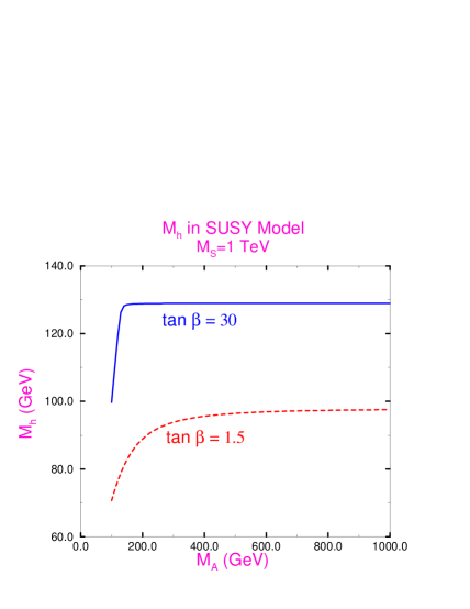
Figure 1: Mass of the lightest neutral Higgs boson as a function of the pseudoscalar mass, $M_{A}$, and $\tan\beta$. This figure includes radiative corrections to the Higgs mass[28], assumes a common scalar mass of $1~{}TeV$, and neglects mixing effects, ($A_{i}=\mu=0$).

When the electroweak symmetry is broken, the $W$ gauge boson gets a mass which is fixed by $v_{1}$ and $v_{2}$,

$$M_{W}^{2}={g^{2}\over 2}(v_{1}^{2}+v_{2}^{2})\quad.$$ (23)

Before the symmetry was broken, the $2$ complex $SU(2)_{L}$ Higgs doublets had $8$ degrees of freedom. Three of these were absorbed to give the $W$ and $Z$ gauge bosons their masses, leaving $5$ physical degrees of freedom. There is now a charged Higgs boson, $H^{\pm}$, a CP -odd neutral Higgs boson, $A$, and $2$ CP-even neutral Higgs bosons, $h$ and $H$. After fixing $v_{1}^{2}+v_{2}^{2}$ such that the $W$ gets the correct mass, the Higgs sector is then described by $2$ additional parameters which can be chosen however you like. The usual choice is

$$\tan\beta\equiv{v_{2}\over v_{1}}$$ (24)

and $M_{A}$, the mass of the pseudoscalar Higgs boson. Once these two parameters are given, then the masses of the remaining Higgs bosons can be calculated in terms of $M_{A}$ and $\tan\beta$. Note that we can chose $0\leq\beta\leq{\pi\over 2}$ since we have chosen $v_{1},v_{2}>0$.

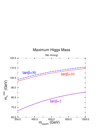
Figure 2: Maximum value of the lightest Higgs boson mass as a function of the squark mass including radiative corrections.[28] (We have assumed degenerate squarks and set the mixing parameters $A_{i}=\mu=0$.)

It is straightforward to find the physical Higgs bosons and their masses in terms of the parameters of Eq. 19. Details can be found in Ref. [hhg]. The neutral Higgs masses are found by diagonalizing the $2\times 2$ Higgs mass matrix and by convention, $h$ is taken to be the lighter of the neutral Higgs. The pseudoscalar mass is given by,

$$M_{A}^{2}={2\mid\mu B\mid\over\sin 2\beta},$$ (25)

and the charged scalar mass is,

$$M_{H^{\pm}}^{2}=M_{W}^{2}+M_{A}^{2}\quad.$$ (26)

We see that at tree level[hbound], Eq. 19 gives important predictions about the relative masses of the Higgs bosons,

$$M_{H^{+}} > M_{W}$$

$$M_{H} > M_{Z}$$

$$M_{h} < M_{A}$$

$$M_{h} < M_{Z}\mid\cos 2\beta\mid\quad.$$ (27)

These relations yield the desirable prediction that the lightest neutral Higgs boson is lighter than the $Z$ boson and so must be observable at LEPII. Unfortunately (for experimentalists at least!) it was realized several years ago that loop corrections to the relations of Eq. 27 are large. In fact the corrections to $M_{h}^{2}$ grow like $G_{F}M_{T}^{4}$ and receive contributions from loops with both top quarks and squarks. In a model with unbroken supersymmetry, these contributions would cancel. Since the supersymmetry has been broken by splitting the masses of the fermions and their scalar partners, the neutral Higgs boson masses become at one- loop,[massloop]

$$M_{h,H}^{2}={1\over 2}\biggl{\{}M_{A}^{2}+M_{Z}^{2}+{\epsilon_{h}\over\sin^{2}\beta}\pm\biggl{[}\biggl{(}M_{A}^{2}-M_{Z}^{2})\cos 2\beta+{\epsilon_{h}\over\sin^{2}\beta}\biggr{)}^{2}+\biggl{(}M_{A}^{2}+M_{Z}^{2}\biggr{)}^{2}\sin^{2}2\beta\biggr{]}^{1/2}\biggr{\}}$$ (28)

where $\epsilon_{h}$ is the contribution of the one-loop corrections,

$$\epsilon_{h}\equiv{3G_{F}\over\sqrt{2}\pi^{2}}M_{T}^{4}\log\biggl{(}{{\tilde{m}}^{2}\over M_{T}^{2}}\biggr{)}\quad.$$ (29)

We have assumed that all of the squarks have equal masses, ${\tilde{m}}$, and have neglected the smaller effects from the mixing parameters, $A_{i}$ and $\mu$. In Fig. 1, we show the lightest Higgs boson mass as a function of the assumed common squark mass,${\tilde{m}}$, and for two values of $\tan\beta$. For $\tan\beta>1$, the mass eigenvalues increase monotonically with increasing $M_{A}$ and give an upper bound to the mass of the lightest Higgs boson,

$$M_{h}^{2}<M_{Z}^{2}\cos^{2}2\beta+\epsilon_{h}\quad.$$ (30)

The corrections from $\epsilon_{h}$ are always positive and increase the mass of the lightest neutral Higgs boson with increasing top quark mass. From Fig. 1, we see that $M_{h}$ obtains its maximal value for rather modest values of the pseudoscalar mass, $M_{A}>300~{}GeV$. The radiative corrections to the charged Higgs mass-squared are proportional to $M_{T}^{2}$ and so are much smaller than the corrections to the neutral masses.

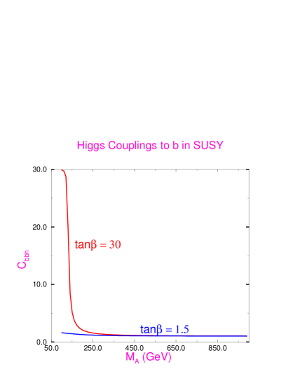
Figure 3: Coupling of the lightest Higgs boson to charge $-1/3$ quarks including radiative corrections [28] in terms of the couplings defined in Eq. 32. The value $C_{bbh}=1$ corresponds to the Standard Model coupling of the Higgs boson to charge $-1/3$ quarks.

There are many sophisticated analyses[massloop] which include a variety of two-loop effects, renormalization group effects, etc., but the important point is that for given values of $\tan\beta$ and the squark masses, there is an upper bound on the lightest neutral Higgs boson mass. The maximum value of the lightest Higgs mass is shown in Fig. 2 and we see that there is still a light Higgs boson even when radiative corrections are included. For large values of $\tan\beta$ the limit is relatively insensitive to the value of $\tan\beta$ and with a squark mass less than about $1~{}TeV$, the upper limit on the Higgs mass is about $110~{}GeV$. Different approaches can raise this limit slightly to around $130~{}GeV$.

• The minimal SUSY model predicts a neutral Higgs boson with a mass less than around $130~{}GeV$.

Such a mass scale will be accessible at LEPII or the LHC and provides a definitive test of the MSSM.

In a more complicated SUSY model with a richer Higgs structure, this bound will, of course, be changed. However, the requirement that the Higgs self coupling remain perturbative up to the Planck scale gives an upper bound on the lightest SUSY Higgs boson of around $150~{}GeV$ in all models.[quiros] This is a very strong statement. It implies that either there is a relatively light Higgs boson (which would be accessible experimentally at LEPII or the LHC) or else there is some new physics between the weak scale and the Planck scale which causes the Higgs couplings to become non-perturbative.

The Higgs boson couplings to fermions are dictated by the gauge invariance of the superpotential and at lowest order are completely specified in terms of the two parameters, $M_{A}$ and $\tan\beta$. From Eq. 16, we see that the charge $2/3$ quarks get their masses entirely from $v_{2}$, while the charge $-1/3$ quarks receive their masses from $v_{1}$. This is a consequence of the $U(1)$ hypercharge assignments for $H_{1}$ and $H_{2}$ given in Table 1. In the Standard Model, it is possible to give both the up and down quarks mass using a single Higgs doublet. This is because in the Standard Model the up quarks can get their masses from the charge conjugate of the Higgs doublet. Terms involving the charge conjugates of the superfields are not allowed in SUSY models, however, and so a second Higgs doublet with opposite $U(1)$ hypercharge from the first Higgs doublet is necessary in order to give the up quarks mass. Requiring that the fermions have their observed masses fixes the couplings in the superpotential of Eq. 16,[habergun]

$$\lambda_{D} = {gM_{d}\over\sqrt{2}M_{W}\cos\beta}$$

$$\lambda_{U} = {gM_{u}\over\sqrt{2}M_{W}\sin\beta}$$

$$\lambda_{L} = {gM_{l}\over\sqrt{2}M_{W}\cos\beta}\quad,$$ (31)

where $g$ is the $SU(2)_{L}$ gauge coupling, $g^{2}=4\sqrt{2}G_{F}M_{W}^{2}$. We see that the only free parameter in the superpotential now is the Higgs mass parameter, $\mu$, (along with the angle $\beta$ in the $\lambda_{i}$ couplings).

It is convenient to write the couplings for the neutral Higgs boson to the fermions in terms of the Standard Model Higgs couplings,

$${\cal L}=-{gm_{i}\over 2M_{W}}\biggl{[}C_{ffh}{\overline{f}}_{i}f_{i}h+C_{ffH}{\overline{f}}_{i}f_{i}H+C_{ffA}{\overline{f}}_{i}\gamma_{5}f_{i}A\biggr{]},$$ (32)

where $C_{ffh}$ is $1$ for a Standard Model Higgs boson. The $C_{ffh}$ are given in Table 3 and plotted in Figs. 3 and 4 as a function of $M_{A}$. We see that for small $M_{A}$ and large $\tan\beta$, the couplings of the neutral Higgs boson to fermions can be significantly different from the Standard Model couplings; the $b$-quark coupling becomes enhanced, while the $t$-quark coupling is suppressed. It is obvious from Figs. 3 and 4 that when $M_{A}$ becomes large the Higgs-fermion couplings approach their standard model values, $C_{ffh}\rightarrow 1$. In fact even for $M_{A}\sim 300~{}GeV$, the Higgs-fermion couplings are very close to their Standard Model values.

Table 3: Higgs Boson Couplings to fermions $f$ $C_{ffh}$ $C_{ffH}$ $C_{ffA}$ $u$ ${\cos\alpha\over\sin\beta}$ ${\sin\alpha\over\sin\beta}$ $\cot\beta$ $d$ $-{\sin\alpha\over\cos\beta}$ ${\cos\alpha\over\cos\beta}$ $\tan\beta$

Figure 4: Coupling of the lightest Higgs boson to charge $2/3$ quarks including radiative corrections [28] in terms of the couplings defined in Eq. 32. The value $C_{tth}=1$ yields the Standard Model coupling of the Higgs boson to charge $2/3$ quarks.

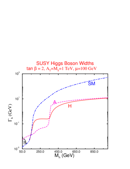
Figure 5: Total SUSY Higgs boson decay widths including two-loop radiative corrections as a function of the Higgs masses. The curve for the lightest Higgs boson is cut off at the maximum $M_{h}$. The program HDECAY [32] was used to obtain this plot.

The Higgs boson couplings to gauge bosons are fixed by the $SU(2)_{L}\times U(1)$ gauge invariance. Some of the phenomenologically important couplings are:

$$Z^{\mu}Z^{\nu}h: {igM_{Z}\over\cos\theta_{W}}\sin(\beta-\alpha)g^{\mu\nu}$$

$$Z^{\mu}Z^{\nu}H: {igM_{Z}\over\cos\theta_{W}}\cos(\beta-\alpha)g^{\mu\nu}$$

$$W^{\mu}W^{\nu}h: igM_{W}\sin(\beta-\alpha)g^{\mu\nu}$$

$$W^{\mu}W^{\nu}H: igM_{W}\cos(\beta-\alpha)g^{\mu\nu}$$

$$Z^{\mu}h(p)A(p^{\prime}): {g\cos(\beta-\alpha)\over 2\cos\theta_{W}}(p+p^{\prime})^{\mu}$$

$$Z^{\mu}H(p)A(p^{\prime}): -{g\sin(\beta-\alpha)\over 2\cos\theta_{W}}(p+p^{\prime})^{\mu}\quad.$$ (33)

We see that the couplings of the Higgs bosons to the gauge bosons all depend on the same angular factor, $\beta-\alpha$. The pseudoscalar, $A$, has no tree level coupling to pairs of gauge bosons. The angle $\beta$ is a free parameter while the neutral Higgs mixing angle, $\alpha$, which enters into many of the couplings, can be found in terms of the physical masses:

$$\tan 2\alpha={(M_{A}^{2}+M_{Z}^{2})\sin 2\beta\over(M_{A}^{2}-M_{Z}^{2})\cos 2\beta+\epsilon_{h}/\sin^{2}\beta}\quad.$$ (34)

With our conventions, $-{\pi\over 2}\leq\alpha\leq 0$. It is clear that the couplings of the SUSY Higgs to gauge bosons are always suppressed relative to those of the Standard Model. A complete set of couplings for the Higgs bosons (including the charged and pseudoscalar Higgs) at tree level can be found in Ref. [hhg]. These couplings completely determine the decay modes of the SUSY Higgs bosons and their experimental signatures. The important point is that (at lowest order) all of the couplings are completely determined in terms of $M_{A}$ and $\tan\beta$. When radiative corrections are included there is a dependence on the squark masses and the mixing parameters of Eq. 18. This dependence is explored in detail in Ref. [lephiggs].

It is an important feature of the MSSM that for large $M_{A}$, the Higgs sector looks like that of the Standard Model. As $M_{A}\rightarrow\infty$, the masses of the charged Higgs bosons, $H^{\pm}$, and the heavier neutral Higgs, $H$, also become large leaving only the lighter Higgs boson, $h$, in the spectrum. In this limit, the couplings of the lighter Higgs boson, $h$, to fermions and gauge bosons take on their Standard Model values. We have,

$$\sin(\beta-\alpha) \rightarrow 1~{}{\hbox{for}}~{}M_{A}\rightarrow\infty$$

$$\cos(\beta-\alpha) \rightarrow 0\quad.$$ (35)

From Eq. 33, we see that the heavier Higgs boson, $H$, decouples from the gauge bosons in the heavy $M_{A}$ limit, while the lighter Higgs boson, $h$, has Standard Model couplings. Figs. 3 and 4 demonstrate that the Standard Model limit is also rapidly approached in the fermion-Higgs couplings for $M_{A}>300~{}GeV$. In the limit of large $M_{A}$, it will thus be exceedingly difficult to differentiate a SUSY Higgs sector from the Standard Model Higgs boson.

• The SUSY Higgs sector with large $M_{A}$ looks like the Standard Model Higgs sector.

The total width of the Higgs boson depends sensitively on $\tan\beta$ and is illustrated in Fig. 5 for $\tan\beta=2$.[squrad] We see that the lightest Higgs boson has a width $\Gamma_{h}\sim 10-100~{}MeV$, while the heavier Higgs boson has a width $\Gamma_{H}\sim.1-1~{}GeV$, which is considerably narrower than the width of the Standard Model Higgs boson with the same mass. (The curve for the lighter Higgs boson is cut off at the kinematic upper limit.) The pseudoscalar, $A$, is also narrower than a Standard Model Higgs boson with the same mass.

The Squark and Slepton Sector

We turn now to a discussion of the scalar partners of the quarks and leptons. The left-handed $SU(2)_{L}$ quark doublet has scalar partners,

$${\tilde{Q}}=\left(\begin{array}[]{c}{\tilde{u}}_{L}\\ {\tilde{d}}_{L}\end{array}\right)\quad.$$ (36)

The right-handed quarks also have scalar partners, ${\tilde{u}}_{R}$ and ${\tilde{d}}_{R}$. The L and R subscripts denote which helicity quark the scalars are partners of– they are for identification purposes only. These are ordinary complex scalars. Before SUSY is broken the fermions and scalars have the same masses and this mass degeneracy is split by the soft mass terms of Eq. 18. The tri-linear $A$ terms allow the scalar partners of the left- and right-handed fermions to mix to form the mass eigenstates. In the top squark sector, the mixing between the scalar partners of the left- and right handed top (the stops), ${\tilde{t}}_{L}$ and ${\tilde{t}}_{R}$, is given by

$$M_{{\tilde{t}}}^{2}=\left(\begin{array}[]{ll}{\tilde{M}}_{Q}^{2}+M_{T}^{2}+M_{Z}^{2}({1\over 2}-{2\over 3}\sin^{2}\theta_{W})\cos 2\beta&M_{T}(A_{T}+\mu\cot\beta)\\ M_{T}(A_{T}+\mu\cot\beta)&{\tilde{M}}_{U}^{2}+M_{T}^{2}+{2\over 3}M_{Z}^{2}\sin^{2}\theta_{W}\cos 2\beta\end{array}\right)\quad.$$ (37)

For the scalars associated with the lighter quarks, the mixing effects will be negligible, since the mixing is proportional to the quark mass, (except if $\tan\beta>>1$, when ${\tilde{b}_{L}}-{\tilde{b}_{R}}$ mixing may be large).

From Eq. 37, we see that there are two important cases to consider. If the soft breaking occurs at a large scale, much greater than $M_{Z}$, $M_{T}$, and $A_{T}$, then all the soft masses will be approximately equal, and we will have $12$ degenerate squarks with mass ${\tilde{m}}\sim{\tilde{M}}_{Q}\sim{\tilde{M}}_{U}\sim{\tilde{M}}_{D}$. On the other hand, if the soft masses and the tri-linear mixing term, $A_{T}$, are on the order of the electroweak scale, then mixing effects become important.

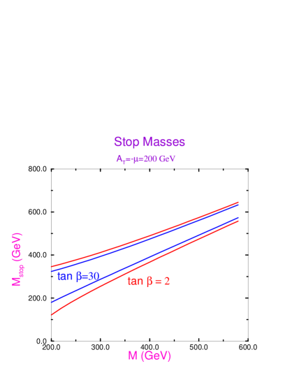
Figure 6: Stop squark masses for large mixing parameters, $A_{T}=\mu=200~{}GeV$, and for $\tan\beta=2$ and $\tan\beta=30$. $M\equiv{\tilde{M}}_{Q}={\tilde{M}}_{u}$ are the squark mass parameters of Eq. 37.

If mixing effects are large, then one of the stop squarks will become the lightest squark, since the mixing effects are proportional to the relevant quark masses and hence will be largest in this sector. The case where the lightest squark is the stop is particularly interesting phenomenologically, and we discuss it in the section on squark mass limits.[stop] In Fig. 6, we show the stop squark masses for ${\tilde{M}}_{Q}={\tilde{M}_{t}}={\tilde{M}_{b}}\equiv{\tilde{m}}$ and for several values of $\tan\beta$. Of course the mixing effects cannot be too large, or the stop squark mass-squared will be driven negative, leading to a breaking of the color $SU(3)$ gauge symmetry. Typically, the requirement that the correct vacuum be chosen leads to a restriction on the mixing parameter on the order of $\mid A_{T}\mid<{\tilde{m}}$.[bagtasi]

The couplings of the squarks to gauge bosons are completely fixed by gauge invariance, with no free parameters. A few examples of the couplings are:

$$\gamma^{\mu}~{}{\tilde{q}}_{L,R}(p)~{}{\tilde{q}}_{L,R}^{*}(p^{\prime}): -ieQ_{q}(p+p^{\prime})^{\mu}$$

$$W^{\mu-}~{}{\tilde{u}}_{L}(p)~{}{\tilde{d}}_{L}^{*}(p^{\prime}): -{ig\over\sqrt{2}}(p+p^{\prime})^{\mu}$$

$$Z^{\mu}~{}{\tilde{q}}_{L,R}(p)~{}{\tilde{q}}_{L,R}^{*}(p^{\prime}): -{ig\over\cos\theta_{W}}\biggl{[}T_{3}-Q_{q}\sin^{2}\theta_{W}\biggr{]}(p+p^{\prime})^{\mu}\quad,$$ (38)

where $T_{3}$ and $Q_{q}$ are the quantum numbers of the corresponding quark. The strength of the interactions are clearly given by the relevant gauge coupling constants. A complete set of Feynman rules can be found in Ref. [hkrep]

The mixing in the slepton sector is analogous to that in the squark sector and we will not pursue it further. From Table 1, we see that the scalar partner of the $\nu_{L}$, ${\tilde{\nu}}_{L}$, has the same gauge quantum numbers as the $H_{2}^{0}$ Higgs boson. It is possible to give ${\tilde{\nu}}_{L}$ a vacuum expectation value and use it to break the electroweak symmetry. Such a vacuum expectation value would break lepton number (and $R$ parity) thereby giving the neutrinos a mass and so its magnitude is severely restricted. [rparity]

The Chargino Sector

There are two charge $1$, spin- ${1\over 2}$ Majorana fermions; ${\tilde{\omega}}^{\pm}$, the fermion partners of the $W^{\pm}$ bosons, and ${\tilde{h}}^{\pm}$, the charged fermion partners of the Higgs boson, termed the Higgsinos. The physical mass states, ${\tilde{\chi}}_{1,2}^{\pm}$, are linear combinations formed by diagonalizing the mass matrix and are usually called charginos. In the ${\tilde{\omega}}^{\pm}-{\tilde{h}}^{\pm}$ basis the chargino mass matrix is,

$$M_{\tilde{\chi}^{\pm}}=\left(\begin{array}[]{cc}M_{2}&\sqrt{2}M_{W}\sin\beta\\ \sqrt{2}M_{W}\cos\beta&-\mu\end{array}\right)\quad.$$ (39)

The physics is extremely sensitive to $M_{2}/\mu$. The mass eigenstates are then,

$$M^{2}_{{\tilde{\chi}}^{\pm}_{1,2}}={1\over 2}\biggl{\{}M_{2}^{2}+2M_{W}^{2}+\mu^{2}\mp\biggl{[}(M_{2}^{2}-\mu^{2})^{2}+4M_{W}^{4}\cos^{2}2\beta+4M_{W}^{2}(M_{2}^{2}+\mu^{2}-2M_{2}\mu\sin^{2}\beta\biggr{]}^{1/2}\biggr{\}}.$$ (40)

By convention $M_{{\tilde{\chi}}_{1}^{\pm}}$ is the lighter chargino.

The Neutralino Sector

In the neutral fermion sector, the neutral fermion partners of the $B$ and $W^{3}$ gauge bosons, ${\tilde{b}}$ and ${\tilde{\omega}}^{3}$, can mix with the neutral fermion partners of the Higgs bosons, ${\tilde{h}}_{1}^{0},{\tilde{h}}_{2}^{0}$. Hence the physical states, ${\tilde{\chi}}_{i}^{0}$, are found by diagonalizing the $4\times 4$ mass matrix,

$$M_{\tilde{\chi}_{i}^{0}}=\left(\begin{array}[]{cccc}M_{1}&0&-M_{Z}\cos\beta\sin\theta_{W}&M_{Z}\sin\beta\sin\theta_{W}\\ 0&M_{2}&M_{Z}\cos\beta\cos\theta_{W}&-M_{Z}\sin\beta\cos\theta_{W}\\ -M_{Z}\cos\beta\sin\theta_{W}&M_{Z}\cos\beta\sin\theta_{W}&0&\mu\\ M_{Z}\sin\beta\sin\theta_{W}&-M_{Z}\sin\beta\cos\theta_{W}&\mu&0\end{array}\right)$$ (41)

where $\theta_{W}$ is the electroweak mixing angle and we work in the ${\tilde{b}},{\tilde{\omega}}^{3},{\tilde{h}}_{1}^{0},{\tilde{h}}_{2}^{0}$ basis. The physical masses can be defined to be positive and by convention, $M_{{\tilde{\chi}}_{1}^{0}}<M_{{\tilde{\chi}}_{2}^{0}}<M_{{\tilde{\chi}}_{3}^{0}}<M_{{\tilde{\chi}}_{4}^{0}}$. In general, the mass eigenstates do not correspond to a photino, (a fermion partner of the photon), or a zino, (a fermion partner of the $Z$), but are complicated mixtures of the states. The photino is only a mass eigenstate if $M_{1}=M_{2}$. Physics involving the neutralinos therefore depends on $M_{1}$, $M_{2}$, $\mu$, and $\tan\beta$. The lightest neutralino, ${\tilde{\chi}}_{1}^{0}$, is usually assumed to be the LSP.

WHY DO WE NEED SUSY?

Having introduced the MSSM as an effective theory at the electroweak scale and briefly discussed the various new particles and interactions of the model, I turn now to a discussion of the reasons for constructing a SUSY theory in the first place. We have already discussed the cancellation of the quadratic divergences, which is automatic in a supersymmetric model. There are, however, many other reasons why theorists are excited about supersymmetry. Theorists will often state that the mathematics of a supersymmetric model is ${\it beautiful}$. However, in my mind, the beauty of supersymmetry is largely obscured by the ugliness of the SUSY breaking sector which we have introduced, and it is therefore essential to have a solid motivation for studying SUSY theories.

Coupling constants run!

In a gauge theory, coupling constants scale with energy according to the relevant $\beta$-function. Hence, having measured a coupling constant at one energy scale, its value at any other energy can be predicted. At one loop,

$${1\over\alpha_{i}(Q)}={1\over\alpha_{i}(M)}+{b_{i}\over 2\pi}\log\biggl{(}{M\over Q}\biggr{)}\quad.$$ (42)

In the Standard (non-supersymmetric) Model, the coefficients $b_{i}$ are given by,

$$b_{1} = {4\over 3}N_{g}+{N_{H}\over 10}$$

$$b_{2} = -{22\over 3}+{4\over 3}N_{g}+{N_{H}\over 6}$$

$$b_{3} = -11+{4\over 3}N_{g}\quad,$$ (43)

where $N_{g}=3$ is the number of generations and $N_{H}=1$ is the number of Higgs doublets. The evolution of the coupling constants is seen to be sensitive to the particle content of the theory. We can take $M=M_{Z}$ in Eq. 42, input the measured values of the coupling constants at the $Z$-pole and evolve the couplings to high energy. The result is shown in Fig. 7. There is obviously no meeting of the coupling constants at high energy.

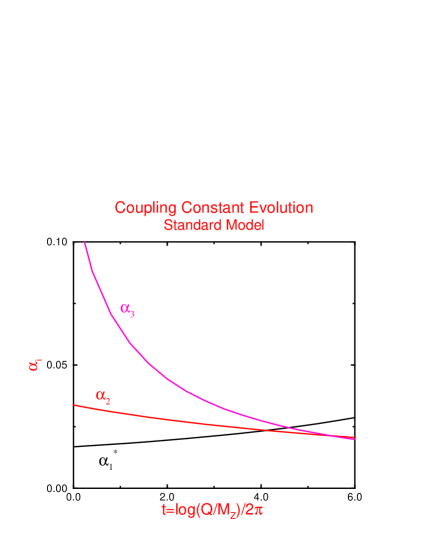
Figure 7: Evolution of the gauge coupling constants in the Standard Model from the experimentally measured values at the $Z$-pole. $\alpha_{1}^{*}\equiv 5/3\alpha_{1}$, since this is the relevant coupling in Grand Unified Theories.

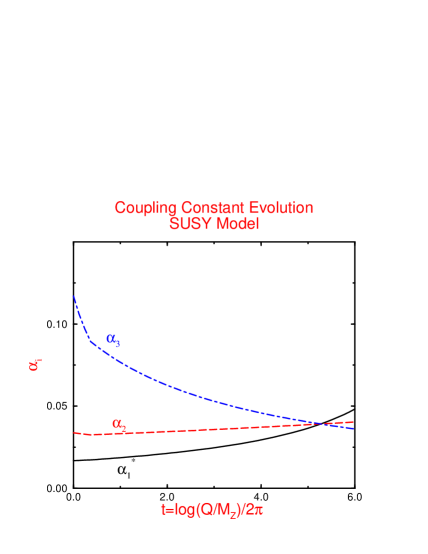
Figure 8: Evolution of the coupling constants in a low energy SUSY model from the experimentally measured values at the $Z$-pole. The SUSY thresholds are taken to be at $1~{}TeV$. $\alpha_{1}^{*}\equiv 5/3\alpha_{1}$, since this is the relevant coupling in Grand Unified Theories.

If the theory is supersymmetric, then the spectrum is different and the new particles contribute to the evolution of the coupling constants. In this case we have,[betafuns]

$$b_{1} = 2N_{g}+{3\over 10}N_{H}$$

$$b_{2} = -6+2N_{g}+{N_{h}\over 2}$$

$$b_{3} = -9+2N_{g}\quad.$$ (44)

Because a SUSY model of necessity contains two Higgs doublets, we have $N_{H}=2$. If we assume that the mass of all the SUSY particles is around $1~{}TeV$, then the coupling constants scale as shown in Fig. 8. We see that the coupling constants meet at a scale around $10^{16}$ GeV.[early, unif, ccunif] This meeting of the coupling constants is a necessary feature of a Grand Unified Theory (GUT).

• SUSY theories can be naturally incorporated into Grand Unified Theories.

There are many variations on this theme including two loop beta functions, effects from passing through SUSY particle thresholds, etc., but they all allow us to take the picture of SUSY as resulting from a GUT theory seriously.[ccunif, jb]

SUSY GUTS

The observation that the measured coupling constants tend to meet at a point when evolved to high energy assuming the $\beta$-function of a low energy SUSY model has led to widespread acceptance of a standard SUSY GUT model. We assume that the $SU(3)\times SU(2)_{L}\times U(1)$ gauge coupling constants are unified at a high scale $M_{X}\sim 10^{16}~{}GeV$:

$$\sqrt{{5\over 3}}g_{1}(M_{X})=g_{2}(M_{X})=g_{3}(M_{X})\equiv g_{X}\quad.$$ (45)

The gaugino masses, $M_{i}$, are also assumed to unify,

$$M_{i}(M_{X})\equiv m_{1/2}\quad.$$ (46)

At lowest order, the gaugino masses then scale in the same way as the corresponding coupling constants,

$$M_{i}(M_{W})=m_{1/2}{g_{i}^{2}(M_{W})\over g_{X}^{2}}$$ (47)

yielding

$$M_{2} = {\alpha\over\sin^{2}\theta_{W}}{1\over\alpha_{s}}M_{3}$$

$$M_{1} = {5\over 3}\tan^{2}\theta_{W}M_{2}\quad.$$ (48)

The gluino mass is always the heaviest of the gaugino masses. This relationship between the gaugino masses is a fairly robust prediction of SUSY GUTS and persists in models where the supersymmetry is broken dynamically.[snow, mess]

Typical SUSY GUTS also assume that there is a common scalar mass at $M_{X}$,

$$m_{1}^{2}(M_{X})= m_{2}^{2}(M_{X})\equiv m_{0}^{2}$$

$${\tilde{M}}_{Q}^{2}(M_{X})={\tilde{M}}_{d}^{2}(M_{X})= {\tilde{M}}_{u}(M_{X})= {\tilde{M}}_{L}^{2}(M_{X})={\tilde{M}}_{e}^{2}(M_{X})\equiv m_{0}^{2}\quad.$$ (49)

The neutral Higgs boson masses at $M_{X}$ are then $M_{h,H}^{2}=m_{0}^{2}+\mu^{2}$. As a final simplifying assumption, a common $A$ parameter is assumed,

$$A_{T}(M_{X})=A_{b}(M_{X})=....\equiv A_{0}\quad.$$ (50)

With these assumptions, the SUSY sector is completely described by 5 input parameters at the GUT scale,[fp]

1. A common scalar mass, $m_{0}$.

2. A common gaugino mass, $m_{1/2}$.

3. A common trilinear coupling, $A_{0}$.

4. A Higgs mass parameter, $\mu$.

5. A Higgs mixing parameter, $B$.

This set of assumptions is often called the “superstring inspired SUSY GUT” or SUGRA (although the connection with superstrings and/or supergravity is mostly wishful thinking) or the “constrained MSSM” (CMSSM). Although this framework is somewhat ${\it ad~{}hoc}$, it does provide guidance to reduce the immense parameter space of a SUSY model. In actual practice, these relationships are satisfied only in the simplest models.

The strategy is now to input the $5$ parameters given above at $M_{X}$ and to use the renormalization group equations to evolve the parameters to $M_{W}$. In fact, the requirement that the $Z$ boson obtain its measured value when the parameters are evaluated at low energy can be used to restrict $\mid\mu B\mid$, leaving the $sign(\mu)$ as a free parameter. We can also trade the parameter $B$ for $\tan\beta$. In this way the parameters of the model become

$$m_{0},m_{1/2},A_{0},\tan\beta,{\rm sign}(\mu)\quad.$$ (51)

This form of a SUSY theory is extremely predictive, as the entire low energy spectrum is predicted in terms of a few input parameters. Within this scenario, contours for the various SUSY particle masses can be found as a function of $m_{0}$ and $m_{1/2}$ for given values of $\tan\beta$, $A_{0}$ and ${\rm sign}(\mu)$.[jb, fp]

It is instructive to study the scalar masses within this scenario. The evolution of the sleptons between $M_{X}$ and $M_{W}$ is small and we have the approximate result for the slepton masses,[xerxes, jb]

$${\tilde{M}}_{L}(M_{W})^{2}\sim{\tilde{M}}_{e}(M_{W})^{2}\sim m_{0}^{2},$$ (52)

while the squark masses are roughly

$${\tilde{M}}_{q}^{2}(M_{W})\sim m_{0}^{2}+4m_{1/2}^{2}\quad.$$ (53)

Since the squarks have strong interactions, (which drives the masses upwards), their masses at the weak scale tend to be larger than the sleptons. Once all the particle masses have been computed in this scheme, then their production cross sections and decay rates at any given accelerator can be computed unambiguously.

Changing the input parameters at $M_{X}$ (for example, assuming non-universal scalar masses) of course changes the phenomenology at the weak scale. A preliminary investigation of the sensitivity of the low energy predictions to these assumptions has been made in Ref. [snow]. For now, we will consider the Grand Unified Model described above as a starting point for phenomenological investigations into SUSY and hope that the general search strategies developed for this model will be applicable to other models.

Electroweak Symmetry Breaking

The simple SUSY model described above has the appealing feature that it explains the mechanism of electroweak symmetry breaking. Below, we sketch the argument.

In the Standard Model (non-supersymmetric) with a single Higgs field, $\phi$, the scalar potential is given by:

$$V(\phi)=\mu^{2}\phi^{2}+\lambda\phi^{4}\quad.$$ (54)

By convention, $\lambda>0$. If $\mu^{2}>0$, then $V(\phi)>0$ for all $\phi$ not equal to $0$ and there is no electroweak symmetry breaking. If, however, $\mu^{2}<0$, then the minimum of the potential is not at $\phi=0$ and the potential has the familiar Mexican hat shape. When the Lagrangian is expressed in terms of the physical field, $\phi^{\prime}\equiv\phi-v$, which has zero vacuum expectation value, then the electroweak symmetry is broken and the $W$ and $Z$ gauge bosons acquire non-zero masses. We saw in the previous sections that this same mechanism gives the $W$ and $Z$ gauge bosons their masses in the MSSM. This simple picture leaves one looming question:

$${\rm Why~{}is~{}\mu^{2}<0?}$$

It is this question which the SUSY GUT models can answer.

In the minimal SUGRA model which we have described above, the neutral Higgs bosons both have masses, $M_{h,H}^{2}=m_{0}^{2}+\mu^{2}$, at $M_{X}$ while the squarks and sleptons have mass $m_{0}$ at $M_{X}$. Clearly, at $M_{X}$, the electroweak symmetry is not broken since the Higgs bosons have positive mass-squared. The masses scale with energy according to the renormalization group equations.[yukren] If we neglect gauge couplings and consider only the scaling of the third generation scalars we have,[ewsbtop]

$${d\over d\log(Q)}\left(\begin{array}[]{c}M_{h}^{2}\\ {\tilde{M}}_{t_{R}}^{2}\\ {\tilde{M}}_{Q_{L}^{3}}^{2}\end{array}\right)=-{8\alpha_{s}\over 3\pi}M_{3}^{2}\left(\begin{array}[]{c}0\\ 1\\ 1\end{array}\right)+{\lambda_{T}^{2}\over 8\pi^{2}}\biggl{(}{\tilde{M}}_{Q_{L}^{3}}^{2}+{\tilde{M}}_{t_{R}}^{2}+M_{h}^{2}+A_{T}^{2}\biggr{)}\left(\begin{array}[]{c}3\\ 2\\ 1\end{array}\right)\quad,$$ (55)

where ${\tilde{Q}}_{L}^{3}$ is the $SU(2)_{L}$ doublet containing ${\tilde{t}}_{L}$ and ${\tilde{b}}_{L}$, $h$ is the lightest Higgs boson, $\lambda_{T}$ is the top quark Yukawa coupling constant given in Eq. 31, and $Q$ is the effective scale at which the masses are measured. The signs are such that the Yukawa interactions (proportional to $M_{T}$) decrease the masses, while the gaugino interactions increase the masses. Because of the $3-2-1$ structure of the last term in Eq. 55, the Higgs mass decreases faster than the squark masses and it is possible to drive $M_{h}^{2}<0$ at low energy, while keeping ${\tilde{M}}_{Q_{L}^{3}}^{2}$ and ${\tilde{M}}_{t_{R}}^{2}$ positive. A generic set of scalar masses in a typical SUSY GUT model is shown in Fig. 9. We can clearly see that the lightest Higgs boson mass becomes negative around the electroweak scale.[masssamp]

For large $\lambda_{T}$, we have the approximate solution,

$$M_{h}^{2}(Q)=M_{h}^{2}(M_{X})-{3\over 8\pi^{2}}\lambda_{T}^{2}({\tilde{M}}^{2}_{Q_{L}^{3}}+{\tilde{M}}_{t_{R}}^{2}+M_{h}^{2}+A_{T}^{2})\log\biggl{(}{M_{X}\over Q}\biggr{)}\quad.$$ (56)

Hence the larger $M_{T}$ is, the faster $M_{h}^{2}$ goes negative. This of course generates electroweak symmetry breaking. If $M_{T}$ were light, $M_{h}^{2}$ would remain positive.[ewsbtop] This observation was made ten years ago when we thought the top quark was light, ($\sim 40~{}GeV$). At that time it was ignored as not being phenomenologically relevant. In fact, this mechanism only works for $M_{T}\sim 175~{}GeV$!

• SUSY GUTS can explain electroweak symmetry breaking. The lightest Higgs boson mass is negative, $m_{h}^{2}<0$, because $M_{T}$ is large.

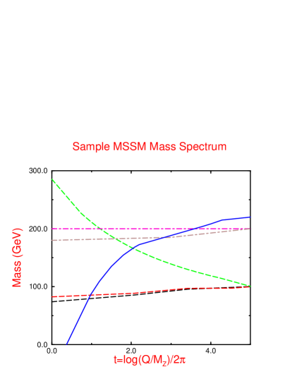
Figure 9: Sample masses of SUSY particles in a SUSY GUT. At the GUT scale $M_{X}$, we have taken $m_{0}=200~{}GeV,m_{1/2}=100~{}GeV,\mu=100~{}GeV$ and $A_{i}=0$. The solid line is the lightest neutral Higgs boson mass. The dashed lines are the gaugino masses (the largest is the gluino) and the dot-dashed lines are typical squark masses.

The $3-2-1$ structure of Eq. 55 drives $M_{h}^{2}$ negative faster than the squark masses. This is important because driving the squark mass negative would have the undesired effect of breaking the color $SU(3)$ symmetry. The requirement that the electroweak symmetry breaking occur through the renormalization group scaling of the Higgs boson mass, (as given in Eq. 55) also restricts the allowed values of $\tan\beta$ to $\tan\beta>1$. (Remember that $\lambda_{T}$ depends on $\beta$ through Eq. 31.)

Fixed Point Interactions

In the previous subsection we saw that a large top quark mass could generate electroweak symmetry breaking in a SUSY GUT model. Here we show that the simplest SUSY GUT actually ${\it predicts}$ a large top quark mass.

The top quark mass is determined in terms of its Yukawa coupling and scales with energy, $Q$,[btau]

$$\lambda_{T}(Q)={M_{T}(Q)\over M_{W}}{g\over\sqrt{2}\sin\beta}\quad.$$ (57)

Including both the gauge couplings and the Yukawa couplings to the $t$- and $b$- quarks, the scaling is:

$${d\lambda_{T}\over d\log(Q)}={\lambda_{T}\over 16\pi^{2}}\biggl{\{}-{13\over 9}g_{1}^{2}-3g_{2}^{2}-{16\over 3}g_{3}^{2}+6\lambda_{T}^{2}+\lambda_{B}^{2}\biggr{\}}\quad.$$ (58)

To a good approximation, we can consider only the contributions from the strong coupling constant, $g_{3}$, and the top quark Yukawa coupling, $\lambda_{T}$. If we begin our scaling at $M_{X}$ and evolve $\lambda_{T}$ to lower energy, we will come to a point where the evolution of the Yukawa coupling stops,

$${d\lambda_{T}\over d\log(Q)}=0\quad.$$ (59)

At this point we have roughly,

$$-{16\over 3}g_{3}^{2}+6\lambda_{T}^{2}=0$$ (60)

which gives,

$$\lambda_{T}\sim{4\over 3}\sqrt{2\pi\alpha_{s}}\sim 1,$$ (61)

or

$$M_{T}\sim(200~{}GeV)\sin\beta\quad.$$ (62)

This point where the top quark mass stops evolving is called a ${\it fixed~{}point}$. What this means is that no matter what the initial condition for $\lambda_{T}$ is at $M_{X}$, it will always evolve to give the same value at low energy. For $\tan\beta\sim 2$, the fixed point value for the top quark mass is close to the experimental value. More sophisticated analyses do not change this picture substantially.

• SUSY GUTS can naturally accommodate a large top quark mass for $\tan\beta\sim 1-3.$

$b-\tau$ Unification

The unification of the $b$- and $\tau$- Yukawa coupling constants, $\lambda_{B}$ and $\lambda_{\tau}$, at the GUT scale is a concept much beloved by theorists since

$$\lambda_{B}(M_{X})=\lambda_{\tau}(M_{X})$$ (63)

occurs naturally in many GUT models. Requiring that the $b$ quark have its experimental value at low energy leads to a prediction for the top quark mass in terms of $\tan\beta$. There are two solutions which yield $M_{T}=175~{}GeV$,[btau]

$$\tan\beta \sim 1$$

$${\rm or}\quad\tan\beta \sim {M_{T}\over M_{b}}\quad.$$ (64)

The first solution roughly corresponds to the fixed point solution of the previous subsection. The second solution with $\tan\beta\sim 35$ has interesting phenomenological consequences, since for large $\tan\beta$ the coupling of the lightest Higgs boson to $b$ quarks is enhanced relative to the Standard Model. (See Fig. 3). The values in the $\tan\beta-M_{T}$ plane allowed by $b-\tau$ unification depend sensitively on the exact value of the strong coupling constant, $\alpha_{s}$, used in the evolution and so there is a significant uncertainly in the prediction.

• SUSY GUTs allow for the unification of the $b-\tau$ Yukawa coupling constants at the GUT scale along with the experimentally observed value for the top quark mass.

Similar relationships to Eq. 63 involving the first two generations do not work.

Comments

We see that SUSY plus grand unification has many desirable features and can explain a lot:

1. There are no troubling quadratic divergences requiring disagreeable cancellations.

2. $M_{T}$ is large because $\lambda_{T}$ evolves from the GUT scale to its fixed point.

3. Electroweak symmetry is broken, $m_{h}^{2}<0$, because $M_{T}$ is large.

4. $b-\tau$ unification can be incorporated, leading to the experimentally observed value for the top quark mass.

Afficianados of SUSY can add many more items to this list.[topten] For instance, the LSP is a leading candidate for cold, dark matter.[dark] The conclusion is inescapable:

SUSY IS  HERE TO  STAY !

SEARCHING FOR SUSY

We begin this section with a description of the effects of SUSY particles on precision measurements and rare decays. We then turn to experimental limits on the various particles and search strategies at current and future machines. A more detailed expose can be found in the lectures of Tata[xerxes] along with up to the minute limits in Refs. [mer, sch].

Indirect Hints for SUSY

One might hope that the precision measurements at the $Z$-pole could be used to garner information on the SUSY particle spectrum. Since the precision electroweak measurements are overwhelmingly in good agreement with the predictions of the Standard Model, it would appear that stringent limits could be placed on the existence of SUSY particles at the weak scale. There are two reasons why this is not the case.

The first is that SUSY is a ${\it decoupling~{}theory}$. With the exception of the Higgs particles, the effects of SUSY particles at the weak scale are suppressed by powers of $M_{W}^{2}/M_{SUSY}^{2}$, where $M_{SUSY}$ is the relevant SUSY mass scale, and so for $M_{SUSY}$ larger than a few hundred $GeV$, the SUSY particles give negligible contributions to electroweak processes. The second reason why there are not stringent limits from precision results at LEP has to do with the Higgs sector. The Higgs bosons are the only particles in the spectrum which do not decouple from the low energy physics when they are very massive. The fits to electroweak data tend to prefer a Higgs boson in the $100~{}GeV$ mass range.[dpf] Since the MSSM requires a light Higgs boson with a mass in this region anyways, the electroweak data is completely consistent with a SUSY model with a light Higgs boson and all other SUSY particles significantly heavier.

Attempts have been made to perform global fits to the electroweak data and to fix the SUSY spectrum this way.[deb, ewsusy] It is possible to obtain a fit where the $\chi^{2}$/degree of freedom is roughly the same as in the Standard Model fit. Although the fits do not yield stringent limits on the SUSY particle masses, they do exhibit several interesting features. They tend to prefer either small $\tan\beta$, $\tan\beta\sim 2$, or relatively large values, $\tan\beta\sim 30$. In addition, the fitted values for the strong coupling constant at $M_{Z}$, $\alpha_{s}(M_{Z})$, are slightly smaller in SUSY models than in the Standard Model. (For $\tan\beta=1.6$, Ref. [deb] finds $\alpha_{s}(M_{Z})=.116\pm.005$ and for $\tan\beta=34$, they find $\alpha_{s}(M_{Z})=.119\pm.005$.) It is clear that all precision electroweak measurements can be accommodated within a SUSY model, but the data show no preference for these models.

There are also numerous indirect limits coming from the effects of SUSY particles on rare decays. Since the SUSY particles circulate in loops, they can affect rare $B$ and $K$ decays (among others). One of the most restrictive limits is from the CLEO measurement of the inclusive decay $B\rightarrow X_{s}\gamma$,[cleo]

$$BR(B\rightarrow X_{s}\gamma)=(2.32\pm.67)\times 10^{-4},\qquad{\rm CLEO}$$ (65)

which is sensitive to loops containing the new particles of a SUSY model. The contribution from $tH^{\pm}$ loops always adds constructively to the Standard Model result and hence non- supersymmetric two- Higgs doublet models are severely restricted by the measurement of $b\rightarrow s\gamma$.

The situation is different in a SUSY model, however, since there are additional contributions from squark-chargino loops, squark- neutralino loops, and squark-gluino loops. The contributions from the squark-neutralino and squark-gluino loops are small and are typically neglected. The dominant contribution from the squark-chargino loops is proportional to $A_{T}\mu$ and thus can have either sign relative to the Standard Model and charged Higgs loop contributions. There will therefore be regions of SUSY parameter space which are excluded depending upon whether there is constructive or destructive interference between the Standard Model/ charged Higgs contributions and the squark-chargino contribution.[bsg] The limit which can be obtained is obviously very sensitive to the sign$(A_{T}\mu)$ and can be easily understood for large $\tan\beta$ where the squark-chargino contribution is completely dominant. Neglecting QCD corrections (which are significant) we have,[bsg2]

$${BR(b\rightarrow s\gamma)\over BR(b\rightarrow ce{\overline{\nu}})}\sim{\mid V_{ts}V_{tb}\mid^{2}\over\mid V_{cb}\mid^{2}}{6\alpha\over\pi}\biggl{\{}C+{M_{T}^{2}A_{T}\mu\over{\tilde{m}}_{T}^{4}}\tan\beta\biggr{\}}^{2}\quad,$$ (66)

where $C$ (positive) is the contribution from the Standard Model and charged Higgs loops and ${\tilde{m}}_{T}$ is the stop mass. For $A_{T}\mu$ positive, this leads to a larger branching ratio, $BR(b\rightarrow s\gamma)$, than in the Standard Model. Since the Standard Model prediction is already somewhat above the measured value, we require $A_{T}\mu<0$ to avoid conflict with the experimental measurement if ${\tilde{m}}_{T}$ is at the electroweak scale and $\tan\beta$ is large. Detailed plots of the allowed regions for various assumptions about $\tan\beta$, $\mu$, and $A_{T}$ are given in Ref. [bb]. Depending on $\tan\beta$ and the sign of $A_{T}\mu$, this process probes stop masses in the $100-300~{}GeV$ region. For large $\tan\beta$, $B\rightarrow X_{s}\gamma$ may probe mass scales as large as a $TeV$.[jhjw]

Another class of important indirect limits on SUSY models comes from flavor changing neutral current (FCNC) processes such as $K^{0}-{\overline{K}}^{0}$ mixing. In general, the matrix which diagonalizes the squark mass matrix is different from that which diagonalizes the quark mass matrix and so there are off-diagonal interactions which can mediate FCNC’s. The contributions from squarks to FCNC processes vanish if the squarks have degenerate masses and so the limits are typically of the form:

$${\Delta{\tilde{m}}^{2}\over{\tilde{m}}^{2}}<{\cal O}(10^{-3})\qquad,$$ (67)

where $\Delta{\tilde{m}}^{2}$ is the mass-squared splitting between the different squarks and ${\tilde{m}}$ is the average squark mass. A detailed discussion of FCNCs in SUSY models and references to the literature is given in Ref. [fcnc]. As a practical matter, the assumption is often made that there are $10$ degenerate squarks, corresponding to the scalar partners of the $u,d,c,s,$ and $b$ quarks, while the stop squarks are allowed to have different masses from the others. This avoids phenomenological problems with FCNCs.

Experimental Limits and Search Strategies

We turn now to a discussion of some of the existing experimental limits on the various SUSY particles and also to the search strategies applicable at present and future accelerators. This section is intended only to give the flavor of how SUSY searches proceed and not as a comprehensive guide. We begin with the Higgs sector.

Observing SUSY Higgs Bosons

The goal in the Higgs sector is to observe the $5$ physical Higgs particles, $h,H,A,H^{\pm}$, and to measure as many couplings as possible to verify that the couplings are those of a SUSY model. The lightest neutral Higgs boson in the minimal SUSY model is unique in the SUSY spectrum because there is an upper bound to its mass,

$$M_{h}<130~{}GeV.$$ (68)

All other SUSY particles in the model can be made arbitrarily heavy just by adjusting the soft SUSY breaking parameters in the model and so be just out of reach of today’s or tomorrow’s accelerators (although if they are heavier than around $1~{}TeV$, much of the motivation for low energy SUSY disappears). The lightest SUSY Higgs boson, however, cannot be much outside the range of LEPII and can almost certainly be observed at the LHC . Hence an extraordinary theoretical effort has gone into the study of the reach of various accelerators in the SUSY Higgs parameter space since in this sector it will be possible to experimentally exclude the MSSM if a light Higgs boson is not observed.

If we find a light neutral Higgs boson, then we want to map out the parameter space to see if we can distinguish it from a Standard Model Higgs boson. The only way to do this is to measure a variety of production and decay modes and attempt to extract the various couplings of the Higgs bosons to fermions and gauge bosons. Since as $M_{A}\rightarrow\infty$, the $h$ couplings approach those of the standard model, there will clearly be a region where the SUSY Higgs boson and the Standard Model Higgs boson are indistinguishable. This is obvious from Figs. 3 and 4.

The search strategies for the SUSY Higgs boson depend sensitively on the Higgs boson branching ratios, which in turn depend on $\tan\beta$. In Figs. 10 and 11, we show the branching ratios for the lightest SUSY Higgs boson, $h$, into some interesting decay modes assuming that there are no SUSY particles light enough for the $h$ to decay into. (These figures include radiative corrections to the branching ratios, which can be important.[squrad]) For a Higgs boson below the $WW$ threshold, the decay into $b{\overline{b}}$ is completely dominant. Unfortunately, there are large QCD backgrounds to this decay mode and so it is often necessary to look at rare decay modes. The branching ratios to $b{\overline{b}}$, $\tau^{+}\tau^{-}$, and $\mu^{+}\mu^{-}$ are relatively insensitive to $\tan\beta$, but the $WW^{*}$, $ZZ^{*}$, and $\gamma\gamma$ rates have strong dependences on $\tan\beta$ as we can see from Figs. 10 and 11.

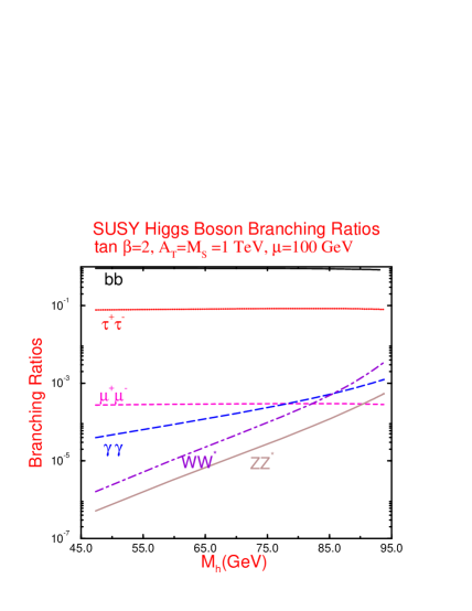
Figure 10: Branching ratios of the lightest Higgs boson assuming decays into other SUSY particles are kinematically forbidden. $WW^{*}$ and $ZZ^{*}$ denote decays with one off-shell gauge boson and $M_{S}$ is a typical squark mass.[32]

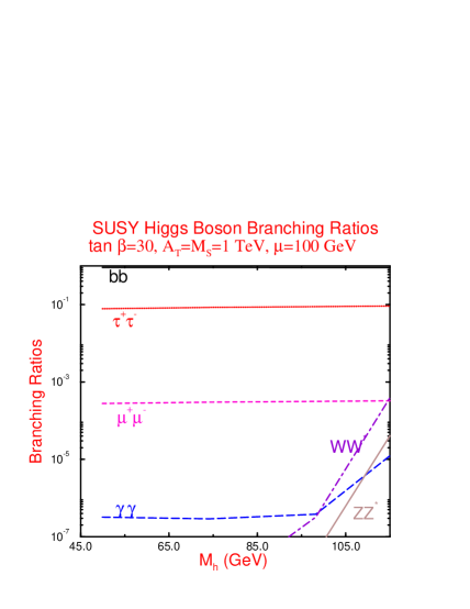
Figure 11: Branching ratios of the lightest Higgs boson assuming decays into other SUSY particles are kinematically forbidden.[32]

Direct limits on SUSY Higgs production have been obtained at LEP by searching for the complementary processes,[lephiggs]

$$e^{+}e^{-} \rightarrow Zh$$

$$e^{+}e^{-} \rightarrow Ah\quad.$$ (69)

From the couplings of Eq. 33, we see that the process $e^{+}e^{-}\rightarrow Zh$ is suppressed by $\sin^{2}(\beta-\alpha)$ relative to the Standard Model Higgs boson production process, while $e^{+}e^{-}\rightarrow Ah$ is proportional to $\cos^{2}(\beta-\alpha)$. The moral is that it is impossible to suppress both processes simultaneously if both the $h$ and the $A$ are kinematically accessible! The experimental searches look for final states with $b$’s and $\tau$’s since these have the largest branching ratios. Because the Higgs sector can be described by the two parameters, $M_{h}$ and $\tan\beta$, searches exclude a region in this plane. (Remember that $M_{A}$ can be expressed in terms of $M_{h}$ and $\tan\beta$ at lowest order. When radiative corrections are included, there will be a dependence on the mixing parameters, $A_{i}$ and $\mu$, and on the squark masses). The LEP searches for Higgs bosons, $e^{+}e^{-}\rightarrow Zh$ and $e^{+}e^{-}\rightarrow AH$, exclude the region, [lephiggs]

$$M_{h}>44~{}GeV,~{}{\rm for~{}any~{}}\tan\beta\quad.$$ (70)

For a given value of $\tan\beta$, there may be a stronger bound. It is important to note that the LEP searches do not leave any window for a very light (on the order of a few $GeV$) Higgs boson. The limit on a SUSY Higgs boson is weaker than the corresponding limit on the Standard Model Higgs boson, $M_{h}^{SM}>65~{}GeV$, due to the suppression in the couplings of the Higgs boson to vector bosons.

Figure 12: Cross sections for $e^{+}e^{-}\rightarrow Zh$ and $e^{+}e^{-}\rightarrow Ah$ at LEP. From Ref. [31].

At LEPII, the cross section for either $Zh$ (small $\tan\beta$) or $Ah$ (large $\tan\beta$) is roughly $.5~{}pb$. With a luminosity of $150/pb/yr$, this leads to $75$ events/yr before the inclusion of branching ratios. Fig. 12 shows the cross sections for two different values of $\tan\beta$ and the complementarity of the two processes can be clearly observed. (The dependence on the top quark mass arises from the inclusion of radiative corrections.)

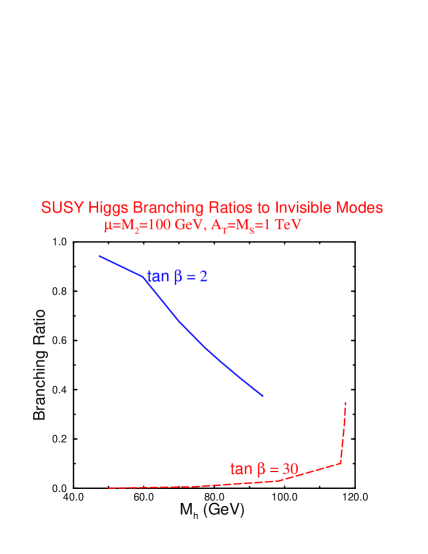
Figure 13: Branching ratio of the lightest Higgs boson to ${\tilde{\chi}}_{1}^{0}{\tilde{\chi}}_{1}^{0}$. The curve with $\tan\beta=30$ has $M_{\chi_{1}^{0}}=33~{}GeV$, while that with $\tan\beta=2$ has $M_{\chi_{1}^{0}}=7~{}GeV$.[32]

The limits on the Higgs boson mass could be substantially altered if there is a significant branching rate into invisible decay modes, such as the neutralinos,

$$h,A\rightarrow{\tilde{\chi}}_{1}^{0}{\tilde{\chi}}_{1}^{0}\quad.$$ (71)

These branching ratios could be as high as $80\%$, but are extremely model dependent since they depend sensitively on the parameters of the neutralino mixing matrix. In Fig. 13, we show the branching ratio of the lightest Higgs boson to ${\tilde{\chi}}_{1}^{0}{\tilde{\chi}}_{1}^{0}$ for several choices of parameters. For $\tan\beta=2$, with the set of parameters which we have chosen, the branching ratio is always greater than $40\%$. If the invisible decay modes are significant, a different search strategy for the Higgs boson must be utilized and LEPII can put a limit on the product of the Higgs boson mixing angles, $\beta-\alpha$, and the branching ratio to invisible modes:

$$R_{1}^{2} \equiv \sin^{2}(\beta-\alpha)BR(h\rightarrow{\hbox{visible}})$$

$$R_{2}^{2} \equiv \sin^{2}(\beta-\alpha)BR(h\rightarrow{\hbox{invisible}})\quad.$$ (72)

For $M_{h}=40~{}GeV$, the $95\%$ confidence level excluded region from LEP is,[lephiggs]

$$R_{1}^{2} < .3$$

$$R_{2}^{2} < .1\quad.$$ (73)

These limits can be reinterpreted in terms of the parameters of the MSSM ($A_{i}$, $\mu$, $M_{2}$, $M_{1}$, ${\tilde{m}}$, etc.) and will be greatly improved at LEPII. For $M_{h}=80~{}GeV$ and an integrated luminosity of $150/pb$ at $\sqrt{s}=192~{}GeV$, the $95\%$ confidence level limit will be:

$$R_{1}^{2} < .1$$

$$R_{2}^{2} < .3\quad.$$ (74)

These limits will significantly restrict the allowed SUSY parameter space.

A $\mu^{+}\mu^{-}$ collider could in principle obtain stringent bounds on a SUSY Higgs boson through its $s$-channel couplings to the Higgs.[bargermm] Since these couplings are proportional to the lepton mass, the $s$-channel Higgs couplings will be much larger at a $\mu^{+}\mu^{-}$ collider than at an $e^{+}e^{-}$ collider. For large $\tan\beta$, the lighter Higgs boson could be found in the process $e^{+}e^{-}\rightarrow Zh$ at LEPII or at an NLC.[lephiggs, nlchiggs] However, for large $\tan\beta$, the coupling of the heavier Higgs boson to gauge boson pairs is highly suppressed, (see Eq. 33), so the $H$ can’t be found through $e^{+}e^{-}\rightarrow ZH$. Instead the $H$ can be found through $\mu^{+}\mu^{-}\rightarrow H\rightarrow b{\overline{b}}$, which is enhanced by the factor $\tan^{2}\beta$ relative to $\mu^{+}\mu^{-}\rightarrow h_{SM}\rightarrow b{\overline{b}}$.

A muon collider could also be very useful for obtaining precision measurements of the lighter Higgs boson mass. The idea is that the $h$ has been discovered through either the process $e^{+}e^{-}\rightarrow Zh$ or $\mu^{+}\mu^{-}\rightarrow Zh$ and so we have a rough idea of the Higgs boson mass. A muon collider could be tuned to sit right on the resonance, $\mu^{+}\mu^{-}\rightarrow h$. By doing an energy scan around the region of the resonance, a precise value of the mass could be obtained due in large part to the narrowness of the muon beam as compared to the beam in an electron collider. (The narrowness of the beam is due to the suppression of synchrotron radiation in a muon collider.)

At the LHC, for most Higgs masses the dominant production mechanism is gluon fusion, $gg\rightarrow h,H$ or $A$. These processes proceed through triangle diagrams with internal $b$ and $t$ quarks and also through squark loops. In the limit in which the top quark is much heavier than the Higgs boson, the top quark contribution is a constant, while the $b$ quark contribution is suppressed by $(M_{b}/v)^{2}\log(M_{h}/M_{b})$ and so only the top quark contribution is numerically important. For large $\tan\beta$, however, the dominance of the top quark loop is overtaken by the large ${\overline{b}}bh$ coupling and the bottom quark contribution becomes important, (as seen in Fig. 3). The production rate is therefore extremely sensitive to $\tan\beta$. Both QCD corrections and squark loops can also be numerically important.[spira] In fact, the QCD corrections increase the rate by a factor between $1.5$ and $2$. The rate for $pp\rightarrow h$ at the LHC is shown in Fig. 14 as a function of $\tan\beta$ for $M_{h}=80~{}GeV$. We see that there are a relatively large number of events. For example, for $M_{h}\sim 80~{}GeV$, the LHC cross section is roughly $100~{}pb$. With a luminosity of $10^{33}/cm^{2}/sec$, this yields $10^{6}$ events/year.

Figure 14: Cross section for production of the lightest SUSY Higgs boson at the LHC as a function of $\tan\beta$.

Unfortunately, there are large backgrounds to the dominant decay modes, ( $b\overline{b},\mu^{+}\mu^{-}$, and $\tau^{+}\tau^{-}$), for a Higgs boson in the $100~{}GeV$ region.[lhchiggs] The decay $h\rightarrow ZZ^{*}$ will be useful, but its branching ratio decreases rapidly with decreasing Higgs mass. In order to cover the region around $M_{h}\sim 80-100~{}GeV$, it will be necessary to look for the Higgs decay to $\gamma\gamma$,

$$gg\rightarrow h,H\rightarrow\gamma\gamma\quad.$$ (75)

(From Figs. 10 and 11, we see that the $BR(h\rightarrow\gamma\gamma)$ is typically $<10^{-3}-10^{-5}$.) This process will be extremely difficult to observe at the LHC due to the small rate and the desire to observe the $h\rightarrow\gamma\gamma$ decay has been one of the driving forces behind the design of both LHC detectors.[lhcprop] For large $M_{A}$, the rate is roughly independent of $\tan\beta$ for $\tan\beta>3$ and can be used to exclude $M_{A}>150~{}GeV$ with the full design luminosity of $3\times 10^{5}/pb$. (With a smaller luminosity of $3\times 10^{4}/{\rm pb}$, the $h\rightarrow\gamma\gamma$ process is sensitive to roughly $M_{A}>270~{}GeV$. See Fig. 15 for the exact region.)

In order to exclude the region with smaller $\tan\beta$, the process $pp\rightarrow Wh\rightarrow l\nu{\overline{b}}b$ can be used.[wm] This process can exclude a region with $M_{A}>100~{}GeV$ and $\tan\beta<4$ (see Fig. 15) and demonstrates the crucial need for $b$-tagging at the LHC in order to cover all regions of SUSY parameter space. In Fig. 15, we see the excluded region formed by combining the LHC and LEP limits.[dfr] A variety of Higgs production and decay channels can be utilized in order to probe the entire $\tan\beta-M_{A}$ plane. The most striking feature of Fig. 15 is the region around $M_{A}\sim 100~{}GeV$ for $\tan\beta>5$ where the lightest Higgs boson cannot be observed. In the region with $M_{A}\sim 100-200~{}GeV$, both the $h{\overline{t}}t$ coupling and the $h\rightarrow\gamma\gamma$ branching ratios are suppressed relative to the Standard Model rates. Furthermore, the dominant decays, $h\rightarrow b{\overline{b}}$ and $h\rightarrow\tau^{+}\tau^{-}$, have large backgrounds from $Z$ decays. It will be necessary to look for the decays of the heavier neutral Higgs boson, $H$, or the pseudoscalar, $A$, to $\tau^{+}\tau^{-}$ pairs in order to probe this region,

$$H,A\rightarrow\tau^{+}\tau^{-}\rightarrow l\nu{\overline{q}}q\quad.$$ (76)

Detector studies by the ATLAS and CMS collaborations suggest that these decay modes may be accessible.

Figure 15: LHC (with low luminosity) and LEPII discovery limits for SUSY Higgs bosons. Figure from Ref. [60].

Finding the Zoo of SUSY Particles

In addition to the multiple Higgs particles associated with SUSY models, there is a whole zoo of other new particles. There are the squarks and gluinos which are produced through the strong interactions and the sleptons, charginos, and neutralinos which are produced weakly.

We begin by discussing some generic signals for supersymmetry. All SUSY particles in a theory with $R$ parity conservation eventually decay to the LSP, which is typically taken to be the lightest neutralino, ${\tilde{\chi}}_{1}^{0}$, although in some models it could be the gravitino.[wein] The LSP’s interactions with matter are extremely weak and so it escapes detection leading to missing energy.

• A basic SUSY signature is missing energy, $E_{T}^{miss}$, from the undetected LSP.

A SUSY model typically produces a cascade of decays, until the final state consists of only the LSP plus jets and leptons. Hence typical final states are:

• $l^{\pm}+{\rm jets}+E_{T}^{miss}$

• $l^{\pm}l^{\pm}+{\rm jets}+E_{T}^{miss}$

• $l^{\pm}l^{\mp}+{\rm jets}+E_{T}^{miss}$  .

Because of the presence of the LSP in the final state, it is not possible to completely reconstruct the masses of the SUSY particles, although a significant amount of information about the masses can be obtained from the event structure.

• A combination of characteristic signatures may determine the SUSY model.

Because the gluinos are Majorana particles, they have some special characteristics which may be useful for their experimental detection. They have the property:

$$\Gamma({\tilde{g}}\rightarrow l^{+}X)=\Gamma({\tilde{g}}\rightarrow l^{-}X)\quad.$$ (77)

Hence gluino pair production can lead to final states with same sign $l^{\pm}l^{\pm}$ pairs.[fp, ssll] The standard model background for this type of signature is rather small.

• Same sign di-lepton pairs are a useful signature for gluino pair production.

Another generic signature for SUSY particles is tri-lepton production.[tri] If we consider the process of chargino-neutralino production,then it is possible to have the process:

$${\tilde{\chi}}_{1}^{\pm}{\tilde{\chi}}_{2}^{0}\rightarrow l\nu{\tilde{\chi}}_{1}^{0}+{\overline{l}}^{\prime}l^{\prime}{\tilde{\chi}}_{1}^{0}\quad.$$ (78)

Again this is a signature with a small standard model background.

In the following sections we will examine several of these signatures in detail. In order to predict the SUSY particle production rates, it is necessary to have an event generator which includes both the production and decays of the SUSY particles. A number of generators exist for both $e^{+}e^{-}$ and hadronic colliders. The physics assumptions of two of the most commonly used event generators for SUSY (ISASUSY and SPYTHIA) are reviewed in Ref. [eventgen].

Chargino and Neutralino Production

As an example of SUSY particle searches, we consider the search for chargino pair production at an electron-positron collider,

$$e^{+}e^{-}\rightarrow{\tilde{\chi}}_{1}^{+}{\tilde{\chi}}_{1}^{-}\quad,$$ (79)

(where ${\tilde{\chi}}_{1}^{\pm}$ are the lightest charginos.) The chargino mass matrix has a contribution from both the fermionic partner of the $W^{\pm}$, ${\tilde{\omega}}^{\pm}$, and from the fermionic partner of the charged Higgs, ${\tilde{h}}^{\pm}$, and so depends on the two unknown parameters in the mass matrix, $\mu$ and $M_{2}$. (See Eq. 40). If $\mid\mu\mid<<M_{2}$, we say the chargino is “Higgsino-like”, while if $\mid\mu\mid>>M_{2}$, it is termed “gaugino-like”. Results are usually presented in terms of the mass of the lightest chargino, $M_{\tilde{\chi}^{+}_{1}}$, and $\mu$.

There are two types of Feynman diagrams contributing to chargino pair production: the first is an $s$-channel exchange of a $\gamma$ or a $Z$, and the second is the $t$-channel exchange of the scalar partner of the neutrino, ${\tilde{\nu}}_{L}$. There is a destructive interference between the two types of diagrams. The largest interference occurs for light ${\tilde{\nu}}_{L}$ and ${\tilde{\chi}}^{\pm}_{1}$ “Gaugino-like”. For light ${\tilde{\nu}}_{L}$, ${\tilde{m}}_{\nu_{L}}<60~{}GeV$, the destructive interference can make the cross section significantly smaller, leading to a weaker limit. For a heavy ${\tilde{\nu}}_{L}$, the interference between the diagrams is small and the production cross section at LEP is $\sigma\sim 6-18~{}pb$ for $M_{{\tilde{\chi}}_{1}^{+}}\sim 60~{}GeV$. Hence any limits which may be obtained will depend on ${\tilde{m}}_{\nu_{L}}$, as well as $\mu$ and $M_{2}$.

The search proceeds by looking for the decay ${\tilde{\chi}}^{\pm}_{1}\rightarrow{\tilde{\chi}}^{0}_{1}l^{\pm}\nu$ . The assumption is made that the ${\tilde{\chi}}^{0}_{1}$ is stable and escapes the detector unseen. Using this technique, ALEPH obtains a limit,[aleph]

$$M_{\tilde{\chi}^{\pm}}>67.8~{}GeV\quad@95\%CL$$

$${\rm For}:\quad\quad\left\{\begin{array}[]{l}~{}m_{\tilde{\nu}_{L}}>200~{}GeV\\ M_{\tilde{\chi}^{\pm}}~{}{\rm gaugino-like},~{}~{}\mid\mu\mid>>M_{2}\quad.\end{array}\right.$$ (80)

This limit is not very sensitive to $\tan\beta$, but is considerably weaker when $\mid\mu\mid\leq 100~{}GeV$. It is clearly important to understand the input assumptions about the various SUSY parameters when interpreting this limit, as is the case with most limits on SUSY particles.

It is interesting to compare the search for charginos and neutralinos at LEP with what is possible at the LHC. At the LHC one clear signature will be,[charg]

$$pp\rightarrow{\tilde{\chi}}^{\pm}_{1}{\tilde{\chi}}^{0}_{2}$$

with,

$${\tilde{\chi}}^{\pm}_{1} \rightarrow l^{\prime\pm}\nu{\tilde{\chi}}_{1}^{0}$$

$${\tilde{\chi}}^{0}_{2} \rightarrow l{\overline{l}}{\tilde{\chi}}_{1}^{0}\quad.$$ (81)

The cross section for this process is $\sigma\sim 1-100~{}pb$ for masses below $1~{}TeV$. This gives a “tri-lepton signature” with three hard, isolated leptons, significant $E_{T}$ and little jet activity.[tri] The dominant Standard Model backgrounds are from $t{\overline{t}}$ production (which can be eliminated by requiring that the 2 fastest leptons have the same sign) and $W^{\pm}Z$ production (which is eliminated by requiring that $M_{ll}\neq M_{Z}$).

To get reliable predictions at a hadron collider, it is not enough to use your Monte Carlo generator to simulate the process of interest (here chargino pair production). One must also simulate all the other SUSY production processes.[multi] It is amusing to note that at the LHC the largest background to chargino and neutralino production is indeed from other SUSY particles, such as squark and gluino production, which also give events with leptons, multi-jets, and missing $E_{T}$. Since the squarks and gluinos are strongly interacting, they will generate more jets and a harder missing $E_{T}$ spectrum than the charginos and neutralinos. This can be used to separate squark and gluino production from the chargino and neutralino production process of interest.[fp]

• The biggest background to SUSY is SUSY itself.

As an example, we quote from a study of the tri-lepton signature at the LHC which assumes relatively light charginos and neutralinos,[fp]

$$M_{{\tilde{\chi}}_{1}^{+}} = 96~{}GeV$$

$$M_{{\tilde{\chi}}_{2}^{0}} = 96~{}GeV$$

$$M_{{\tilde{\chi}}_{1}^{0}} = 45~{}GeV\quad.$$ (82)

Once the SUSY particle masses are specified all the production rates can be computed unambiguously. After cuts, Ref. [fp] finds (at the LHC):

$${\rm Signal}: 41~{}fb$$

$$t{\overline{t}}~{}{\rm bkdg}: 2.4~{}fb$$

$$WZ~{}{\rm bkgd}: .5fb$$

$${\tilde{g}},{\tilde{q}}~{}{\rm bkgd}: 5.6~{}fb,$$ (83)

demonstrating the viability of this signature at the LHC.

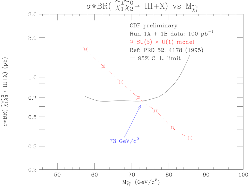
Figure 16: Limits on the tri-lepton signature in the reaction $p{\overline{p}}\rightarrow{\tilde{\chi}}^{\pm}_{1}{\tilde{\chi}}^{0}_{2}$ from CDF. This figure from Ref. [67].

• The tri-lepton signal offers the possibility of untangling the ${\tilde{\chi}}^{+}{\tilde{\chi}}^{0}$ signal from the gluino and squark background.

CDF has searched for this decay chain and we see the results in Fig. 16.[cdflim] Since the branching ratio to tri-leptons depends on the parameters of the chargino and neutralino mass matrix they also show the prediction from a specific Grand Unified Theory. Within this model, the limit translates to $M_{{\tilde{\chi}}_{1}^{\pm}}>73~{}GeV$. This is roughly the same limit as that found at LEP, but involves different assumptions about the parameters of the model.

Aside from observing the process and verifying the existence of charginos and neutralinos, we would also like to obtain a handle on the masses of the SUSY particles. The kinematics are such that,

$$0<M_{ll}<M_{{\tilde{\chi}}^{0}_{2}}-M_{{\tilde{\chi}}^{0}_{1}}\quad,$$ (84)

and hence the distribution $d\sigma/dM_{ll}$ has a sharp cut-off at the kinematic boundary which can be used to obtain information on the masses. Recently, significant progress has been made in our understanding of the capabilities of a hadron collider for extracting values of the SUSY particle masses from different event distributions.[fpsnow]

Squarks, Gluinos, and Sleptons

Squarks and sleptons,(${\tilde{f}}_{i}$), can be produced at both $e^{+}e^{-}$ and hadron colliders. At LEP, they would be pair produced via

$$e^{+}e^{-}\rightarrow\gamma,Z\rightarrow{\tilde{f}}_{i}{\tilde{f}}^{*}_{i}.$$ (85)

If there were a scalar with mass less than half the $Z$ mass, it would increase the total width of the $Z$, $\Gamma_{Z}$. Since $\Gamma_{Z}$ agrees quite precisely with the Standard Model prediction, the measurement of the $Z$ lineshape gives

$${\tilde{m}}>35-40~{}GeV$$ (86)

for squarks and sleptons. The limit from the $Z$ width is particularly important because it is independent of the squark or slepton decay mode and so applies for any model with low energy supersymmetry.

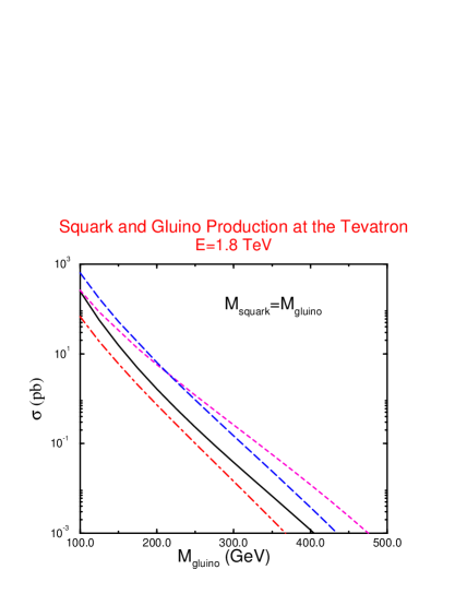
Figure 17: Squark and gluino production at the Tevatron assuming $M_{\tilde{q}}=M_{\tilde{g}}$. The solid line is $p{\overline{p}}\rightarrow{\tilde{g}}{\tilde{g}}$, the dot-dashed ${\tilde{q}}{\tilde{q}}$, the dotted ${\tilde{q}}{\tilde{q}}^{*}$, and the dashed is ${\tilde{q}}{\tilde{g}}$. This figure includes only the Born result and assumes $10$ degenerate squarks.

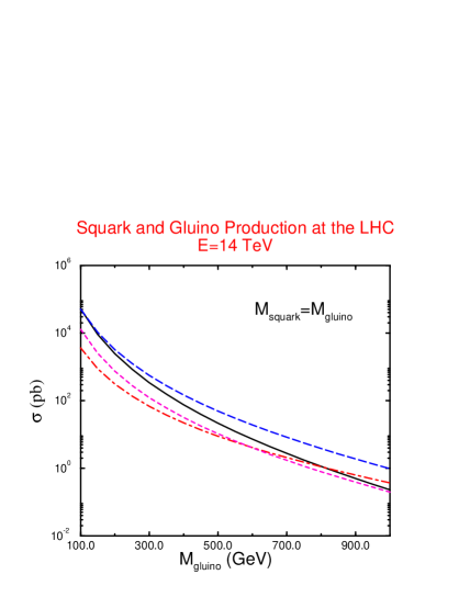
Figure 18: Squark and gluino production at the LHC assuming $M_{\tilde{q}}=M_{\tilde{g}}$. The solid line is $p{\overline{p}}\rightarrow{\tilde{g}}{\tilde{g}}$, the dot-dashed ${\tilde{q}}{\tilde{q}}$, the dotted ${\tilde{q}}{\tilde{q}}^{*}$, and the dashed is ${\tilde{q}}{\tilde{g}}$. This figure includes only the Born result and assumes $10$ degenerate squarks.

There are limits on the direct production of squarks and gluinos from the Tevatron. The rates for squark and gluino production at both the Tevatron and the LHC are shown in Figs. 17 and 18 and analytic expressions for the Born cross sections can be found in Ref. [sigsusy]. The QCD radiative corrections to these process are large and increase the cross sections by up to a factor of two.[squglu] We neglect the mixing effects in the squark mass matrix and assume that there are $10$ degenerate squarks associated with the light quarks. (The top squarks are assumed to be different since here mixing effects are clearly relevant.) The cross sections are significant, around $1~{}pb$ for squarks and gluinos in the few hundred GeV range.

The cleanest signatures for squark and gluino production are jets plus missing $E_{T}$ from the undetected LSP, assumed to be ${\tilde{\chi}}_{1}^{0}$, and jets plus multi leptons plus missing $E_{T}$.[squark] It will clearly be exceedingly difficult to separate the effects of squarks and gluino production, since they both contribute to the same experimental signature. The patterns of squark decays in various scenarios are examined in Ref. [squarkdecay]. To obtain a limit on the gluino mass, we must therefore assume a limit on the squark mass. For 10 degenerate squarks, the limit from the Tevatron is, [mer, pdg]

$$M_{\tilde{q}}>218~{}GeV\qquad{\rm for}M_{\tilde{g}}=M_{\tilde{q}}\quad.$$ (87)

This limit assumes a cascade decay, ${\tilde{q}}\rightarrow(....){\tilde{\chi}}_{1}^{0}$. (There are similar limits for $M_{\tilde{g}}<<M_{\tilde{q}}$ and $M_{\tilde{g}}>>M_{\tilde{q}}$.)

Limits on the stop squark are particularly interesting since in many models it is the lightest squark. There are 2 types of stop squark decays which are relevant. The first is,

$${\tilde{t}}\rightarrow b{\tilde{\chi}}^{+}_{1}\rightarrow bf{\overline{f}}^{\prime}{\tilde{\chi}}_{i}^{0}\quad.$$ (88)

The signal for this decay channel is jets plus missing energy. This signal shares many features with the dominant top quark decay, $t\rightarrow bW^{+}$, and in fact there have been suggestions in the literature that there may be some experimental confusion between the $2$ processes.[barn] Another possible decay chain for the stop squark is

$${\tilde{t}}\rightarrow c{{\tilde{\chi}}_{1}^{0}},$$ (89)

which also leads to jets plus missing energy. The $2$ cases must be analyzed separately. The current limit on the stop squark mass from D0 is shown in Fig. 19.[d0lim] We see that the limit depends sensitively on the mass of the LSP, ${\tilde{\chi}}_{1}^{0}$.

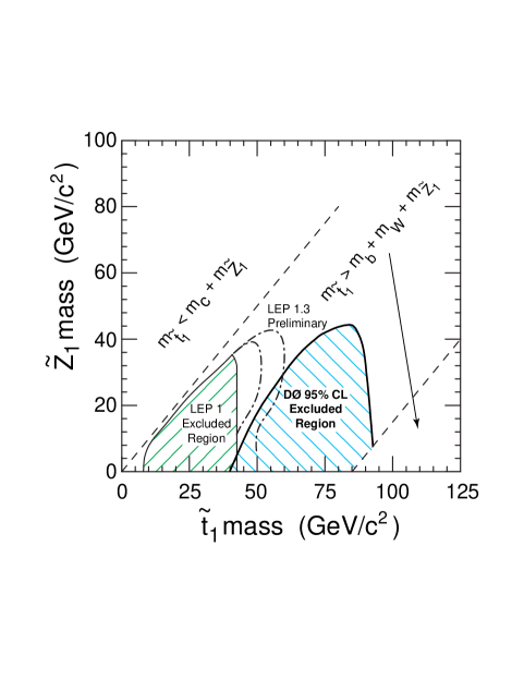
Figure 19: Limit on the lightest stop squark mass here labelled ${\tilde{t}}_{1}$, as a function of the lightest chargino mass (here labelled ${\tilde{Z}}_{1}$) from D0. This figure from Ref. [74].

A spectacular signal for squark pair production which can result from the cascade decays is the production of same sign leptons,

$$pp\rightarrow{\tilde{q}}{\tilde{q}}^{*}\rightarrow(l^{\pm}l^{\pm})+{\rm jets}+E_{T}^{\rm miss}$$ (90)

At the Tevatron with $M_{\tilde{q}}\sim M_{\tilde{g}}\sim 100~{}GeV$, the cross section for jets + $E_{T}^{\rm miss}$ is $\sigma\sim 1~{}pb$, while the rate for $l^{\pm}l^{\pm}+{\rm~{}jets}+E_{T}^{\rm miss}$ is $\sigma\sim.1pb$, which is still significant. The Standard Model background for this signal is quite small.

From the examples we have given, it is clear that searching for SUSY at a hadron collider is particularly challenging since there will typically be many SUSY particles which are kinematically accessible. Hadron colliders thus have a large discovery potential, but it is difficult to separate the various processes. To a large extent, one must trust the generic signatures of supersymmetry: $E_{T}^{\rm miss}$, plus multi-jet and multi-lepton signatures. One will need to observe a signal in many channels in order to verify the consistency of the model.

A Case Study

It is instructive to consider an example of how the discovery of a SUSY particle might occur. Several years ago, CDF presented a single event,

$$p{\overline{p}}\rightarrow e^{+}e^{-}\gamma\gamma+E_{T}^{miss},$$ (91)

for which it was difficult to find a Standard Model explanation.[cdfdata] By now, you all know that events with large missing energy are candidates for SUSY particle production. The scenario which we can construct is then,

$$p{\overline{p}}\rightarrow{\tilde{e}}{\tilde{e}}^{*}\quad,$$ (92)

where ${\tilde{e}}$ is the scalar partner of either the right- or left-handed electron. The production cross section is then fixed unambiguously in terms of the selectron mass. The fact that only one event was seen fixes the selectron mass to be in the $100~{}GeV$ region. The selectron is then assumed to decay to an electron and a neutralino,

$${\tilde{e}}\rightarrow e{\tilde{\chi}}^{0}\quad.$$ (93)

The question which has engendered furious debate is how the neutralino might decay,

$${\tilde{\chi}}^{0}\rightarrow{\tilde{X}}\gamma,$$ (94)

where ${\tilde{X}}$ is either the lightest neutralino or a gravitino.[cdfevent] By examining the kinematics of the event, we could hope to learn about the underlying SUSY model. Unfortunately, examination of the $2$ photon plus $E_{T}^{miss}$ spectrum has produced no more SUSY candidates of the type of Eq. 94.[cdfgam]

CONCLUSIONS

Weak scale supersymmetry is a theory in desperate need of experimental input. The theoretical framework has evolved to a point where predictions for cross sections, branching ratios, and decay signatures can be reliably made. In many cases, calculations exist beyond the leading order in perturbation theory. However, without experimental observation of a SUSY particle or a precision measurement which disagrees with the Standard Model (which could be explained by SUSY particles in loops) there is no way of choosing between the many possible manifestations of low energy SUSY and thereby fixing the parameters in the soft SUSY breaking Lagrangian.

With the coming of LEPII, the Fermilab Main Injector, and the LHC, large regions of SUSY parameter space will be explored and we can only hope that some evidence for supersymmetry will be uncovered. The ball is definitely in the experimentalist’s court !

Acknowledgments

I thank all the students at this school who asked such wonderful questions and really made me think about the experimental consequences of supersymmetry I also thank Tom Ferbel for his superb organization of all the lectures and other happenings at this school. I am grateful to Michael Spira for the use of his program HDECAY for the calculation of the radiatively corrected SUSY Higgs decay widths and also for discussions. Helpful discussions with Frank Paige are also gratefully acknowledged. I am indebted to Ken Kiers for a careful reading of the manuscript. This work has been supported by the DOE under contract number DE-AC02-76-CH-00016.

REFERENCES

1. B. Lee, C. Quigg, and H. Thacker, Phys. Rev. D16 (1977) 1519; D. Dicus and V. Mathur, Phys. Rev. D7 (1973) 3111.

2. G. t’Hooft in Recent Developments in Gauge Theories, eds. G. t’Hooft et.al. (Plenum, N.Y., 1980).

3. J. Amundson et.al., Report of the Supersymmetry Theory Subgroup, Snowmass, 1996, hep-ph/9609374.

4. W. Merritt, Proceedings of the 1996 DPF Meeting, Minneapolis, MN.

5. M. Schmidt, Proceedings of the 1996 DPF Meeting, Minneapolis, MN.

6. H. Haber and G. Kane, Phys. Rep. 117C (1985) 75.

7. J. Bagger, Lectures presented at the 1991 Theoretical Advanced Study Institute, Boulder, CO, June, 1991; Lectures presented at the 1995 Theoretical Advanced Study Institute, Boulder, CO, June, 1995, hep-ph/9604232; H.P. Nilles, Phys. Rep. 110 (1984) 1; H. Haber, Lectures presented at the 1986 Theoretical Advanced Study Institute, Santa Cruz, CA, June, 1986; R. Arnowitt, A. Chamseddine and P. Nath, Applied N=1 Supergravity, (World Scientific, 1984); V. Barger and R. Phillips, Recent Advances in the Superworld, J. Lopez and D. Nanopoulos, Ed. (World Scientific, 1994).

8. X. Tata, Lectures presented at the 1995 Theoretical Advanced Study Institute, QCD and Beyond, Boulder, CO, June, 1995, hep-ph/9510287.

9. H. Murayama and M. Peskin, Ann. Rev. Nucl. Part. Sci. 1996, hep-ex/9606003.

10. G. Anderson, D. Castano, and A. Riotto, hep-ph/9609463, 1996.

11. J. Wess and J. Bagger, Supersymmetry and Supergravity, (Princeton University Press, Princeton, N.J. 1983); P. Fayet and S. Ferrara, Phys. Rep. 32 (1977) 249.

12. D. Gross and R. Jackiw, Phys.Rev. D6 (1972) 477; C. Bouchiat, J. Iliopoulos and P. Meyer, Phys. Lett. B38 (1972) 519; H. Georgi and S. Glashow, Phys. Rev. D6 (1972) 429; L. Alvarez-Gaume and E. Witten, Nucl. Phys. B234 (1983) 269.

13. S. Dimopoulos and H. Georgi, Nucl. Phys. B193 (1981) 150; N. Sakai, Z. Phys. C11 (1981) 153; P. Fayet, Phys. Lett. B69 (1977) 489; B84 (1979) 416.

14. M. Dine, A. Nelson, Y. Shirman, Phys. Rev. D51 (1995) 1362; M. Dine, A. Nelson, Y. Nir, and Y. Shirman, Phys. Rev. D53 (1996) 2658.

15. S. Weinberg, Phys. Rev.D26 (1982) 287; N. Sakai and T. Yanagida, Nucl. Phys. B197 (1982) 533; S. Dimopoulos, S. Raby, and F. Wilczek, Phys. Lett. B112 (1982) 133; J. Ellis, D. Nanopoulos, and S. Rudaz, Nucl. Phys. B202 (1982) 43.

16. C. Carlson, P. Roy, and M. Sher, Phys. Lett B357 (1995) 99.

17. G. Bhattacharyya, hep-ph/9608415 ,1996.

18. G. Farrar and P. Fayet, Phys. Lett. B76 (1978) 575; F. Zwirner, Phys. Lett. 132B (1983) 103; L. Hall and M. Suzuki, Nucl. Phys. B231 (1984) 419; J. Ellis, G. Gelmini, C. Jarlskog, G. Ross, and J. Valle, Phys. Lett. B150 (1985) 142; G. Ross and J. Valle, Phys. Lett. B151 (1985) 375; S. Dawson, Nucl. Phys. B261(1985) 297; S. Dimopoulos and L. Hall, Phys. Lett.B207 (1988) 210.

19. Particle Data Group, Phys. Rev. D 54, (1996) 1.

20. P. Smith et.al., Nucl. Phys. B144 (1979) 525; Nucl Phys. B206 (1982) 333; E. Norman et.al., Phys. Rev. Lett. 58 (1987) 1403; T. Hemmik et.al., Phys. Rev. D41 (1990) 2074; S. Wolfram, Phys. Lett. B82 (1979) 65; C. Dover, T. Gaisser, and G. Steigman, Phys. Rev. Lett. 42 (1979) 1117.

21. H. Baer, C. Kao, and X. Tata, Phys. Rev. D51 (1995) 2180; H. Baer, C. Chen, and X. Tata, hep-ph/9608221, 1996.

22. L. Hall, J. Lykken, and S. Weinberg, Phys. Rev. D 27 (1973) 2359.

23. L. Giradello and M. Grisaru, Nucl. Phys. B194 (1982) 65; K. Harada and N. Sakai, Prog. Theor. Phys. 67 (1982) 67.

24. H. Haber, G. Kane, and T. Sterling, Nucl. Phys. B161 (1979) 493.

25. E. Witten, Nucl. Phys. B185 (1981) 513; M. Dine, W. Fischler, and M. Srednicki, Nucl. Phys. B189 (1981) 575; S. Dimopoulos and S. Raby, Nucl. Phys. B192 (1981) 353; J. Polchinski and L. Susskind, Phys. Rev. D26 (1982) 3661; L. Ibanez and G. Ross, Phys. Lett. B105 (1981) 439.

26. J. Gunion, H. Haber, G. Kane, and S. Dawson, The Higgs Hunter’s Guide (Addison Wesley, Menlo Park, CA) 1990.

27. S. Li and M. Sher, Phys. Lett. B140 (1984) 339; H. Nilles and M. Nusbaumer, Phys. Lett. B145 (1984) 73; J. Gunion and H. Haber, Nucl. Phys. B272 (1986) 1.

28. P. Chankowski, S. Pokorski, and J. Rosiek, Phys. Lett. B274 (1992) 191; B281 (1992) 100; Y. Okada, M. Yamaguchi, and T. Yanagida, Prog. Theor. Phys. 85 (1991) ; Phys. Lett. B262 (1991) 54; J. Espinosa and M. Quiros, Phys. Lett. B267 (1991) 27; Phys. Lett. B266 (1991) 389; H. Haber and R. Hempfling, Phys. Rev. D48 (1993)4280; Phys. Rev. Lett. 66 (1991) 1815; J. Gunion and A. Turski, Phys. Rev. D39 (1989) 2701; D40 (1990) 2333; M. Berger, Phys. Rev. D41 (1990) 225; K. Sasaki, M. Carena and C. Wagner, Nucl. Phys. B381 (1992) 66; R. Barbieri and M. Frigeni, Phys. Lett. B258 (1991) 395; J. Ellis, G. Ridolfi and F. Zwirner, Phys. Lett. B257 (1991) 83; B262 (1991) 477; R. Hempfling and A. Hoang, Phys. Lett. B331 (1994) 99; R. Barbieri, F. Caravaglios, and M. Frigeni, Phys. Lett. B258 (1991)167; H.Haber, R. Hempfling, and H. Hoang, hep-ph/9609331,1996; M.Carena, M. Quiros, and C. Wagner, Nucl. Phys. B461 (1996) 407; M. Carena, J. Espinosa, M. Quiros, and C. Wagner, Phys. Lett. B355 (1995) 209.

29. M. Quiros, XXIV International Meeting on Fundamental Physics: From Tevatron to LHC, Gandia, Spain, 1996, hep-ph/9609392; T. Elliot, S. King, and P. White, Phys. Lett. B305 (1993) 71; G. Kane, C. Kolda, and J. Wells, Phys. Rev. Lett. 70 (1993) 2686.

30. H. Haber and J. Gunion, Nucl. Phys. B272 (1986) 1; Nucl. Phys. B278 (1986) 449; erratum, B402 (1993) 567.

31. M. Carena, P. Zerwas, et.al., Higgs Physics at LEPII, hep-ph/9602250, 1996.

32. The FORTRAN program HDECAY is documented in M. Spira, CERN-TH-95-285, hep-ph/9610350 along with references to the original calculations.

33. S. Mrenna and C. Yuan, Phys. Lett. B367 (1996) 188.

34. J. Bagger, S. Dimopoulos, and E. Masso, Phys. Lett. B156 (1985) 357; Phys. Rev. Lett. 55 (1985) 920; M. Einhorn and D. Jones, Nucl. Phys. B196 (1982) 475.

35. S. Dimopoulos, S. Raby, and F. Wilczek, Phys. Rev. D24 (1981) 1681; U. Amaldi et.al., Phys. Rev. D36 1987 1385; P. Langacker and M. Luo, Phys. Rev. D44 (1991) 514; J. Ellis, S. Kelley, and D. Nanopoulos, Phys. Lett. B260 (1991) 447; U. Amaldi, W. deBoer, and H. Furstenau, Phys. Lett. B260 (1991) 447; N. Sakai, Z. Phys C11 (1982) 153.

36. J. Ellis, S. Kelley, and D. Nanopoulos, Phys. Lett. B260 (1991)131; P. Langacker and M. Luo, Phys. Rev. D44 (1991) 817; U. Amaldi, W. deBoer, and H. Furstenau, Phys. Lett. B260(1991) 447; M. Carena, S. Pokorski, and C. Wagner, Nucl. Phys. B406 (1993) 59; P. Langacker and N. Polonsky, Phys. Rev. D47 (1993) 4028.

37. J. Bagger, K. Matchev, D. Pierce, and R. Zhang, hep-ph/9608444, 1996; J. Bagger, K. Matchev, and D. Pierce, Phys. Lett. B348 (1995) 443; D. Pierce, J. Bagger, K. Matchev, and R. Zhang, hep-ph/9606211, 1996.

38. H. Baer, C. Chen, F. Paige, and X. Tata, Phys. Rev. D54 (1996) 5866; op. cit. D53 (1996) 6241; op.cit. D52 (1995) 1565; D52 (1995) 2746. 39. M. Machacek and M. Vaughn, Nucl. Phys. B222 (1983) 83; C. Ford, D. Jones, P. Stephenson, and M.  Einhorn, Nucl. Phys. B395 (1993) 17.

40. L. Ibanez, Nucl. Phys. B218 (1983) 514; Phys. Lett. B118 (1982) 73; L. Ibanez and G. Ross, Phys. Lett. B110 (1982) 215; J. Ellis, D. Nanopoulos, and K. Tamvakis, Phys. Lett. B121 (1983) 123; L. Alvarez-Gaume, J. Polchinski, and M. Wise, Nucl. Phys. B221 (1983) 495; B. Ananthanarayan, G. Lazarides, and Q. Shafi, Nucl. Phys.D44 (1991) 1613.

41. V. Barger, M. Berger, and P. Ohmann, Phys. Rev. D49 (1994) 4908.

42. B. Pendleton and G. Ross, Phys. Lett. B98 (1981)291; V. Barger, M. Berger, P. Ohmann, and R. Phillips, Phys. Lett. B314 (1993) 351; S. Kelley, J. Lopez, and D. Nanopoulos, Phys. Lett. B274 (1992) 387; M. Carena, M. Olechowski, S. Pokorski, and C. Wagner, Nucl. Phys. B426 (1994) 269; N. Polonsky, Phys. Rev. D54 (1996)4537; N. Polonsky, LMU-TPW-96-04, hep-ph/9602206, 1996..

43. G. Kane in Proceedings of the 28th Rencontres de Moriond, Les Arcs, France, 1993; H. Haber in Workshop on Recent Advances in the Superworld, Woodlands, TX, 1993.

44. H. Goldberg, Phys. Rev. Lett. 50 (1983) 1419; J. Ellis, K. Olive, D. Nanopoulos, J. Hagelin, and M. Srednicki, Nucl. Phys. B328 (1984) 453; M. Drees and M. Nojiri, Phys. Rev.D47 (1993) 376; H. Baer, M. Brhlik, and D. Castano, hep-ph/9607465, 1996.

45. S. Dawson, Invited talk given at the 1996 DPF Meeting, Minneapolis, MN, hep-ph/9609340,1996.

46. W.deBoer et.al., IEKP-KA/96-08, KA-TP-18-96, hep-ph/969209, 1996.

47. P. Chankowski and S. Pokorski, Acta. Phys. Polon. 27 (1996) 1719; G. Kane, R. Stuart, and J. Wells, Phys. Lett. B354 (1995) 350; T. Blazek, M. Carena, S. Raby, and C. Wagner, OHSTPY-HEP-T-96-026, hep-ph/9611217, 1996.

48. M. Alam et.al., (CLEO Collaboration), Phys. Rev. Lett 74 (1995) 2885.

49. S. Bertolini, F. Borzumati, A. Masiero and G. Ridolfi, Nucl. Phys. B353 (1991) 591; R. Barbieri and G. Giudice, Phys. Lett. 309 (1993) 86; P. Nath and R. Arnowitt, Phys. Lett. B336 (1994) 395; G. Kane, C. Kolda, L. Roszkowsi, and J. Wells, Phys. Rev. D49 (1994) 6173; V. Barger, M. Berger, P. Ohmann, and R. Phillips, Phys. Rev. D51 (1995) 2438; B. deCarlos and J. A. Casas, Phys. Lett. B349 (1995) 300, ibid B351 (1995) 604.

50. W. deBoer et.al., IEKP-KA/96-04, hep-ph/9603350, 1996.

51. H. Baer and M. Brhlik, FSU-HEP-961001, hep-ph/9610224, 1996.

52. J. Hewett and J. Wells, SLAC-PUB-7290, hep-ph/9610323, 1996.

53. F. Gabbiani, E. Gabrielli, A. Masiero, and L. Silvestrini, ROM2F/96/21, hep-ph/9604387, 1996; L. Hall, A. Kostelecky, and S. Raby, Nucl. Phys. B267 (1986) 415; L. Hall and L. Randall, Phys. Rev. Lett. 65 (1990) 2939; M. Dine, R. Leigh, and A. Kagan, Phys. Rev. D48 (1993) 4269; Y. Nir and N. Seiberg, Phys. Rev. Lett. B309 (1993) 337 .

54. V. Barger, M. Berger, J. Gunion, and T. Han, hep-ph/9606417, 1996; Proceedings of the 3rd International Conference on Physics Potential and Development of $\mu^{+}\mu^{-}$ Colliders, San Francisco, Dec. 1995, hep-ph/9604334.

55. A. Djouadi et. al., Proceedings of the Workshop Physics with $e^{+}e^{-}$ Linear Colliders, (Annecy-Gran Sasso-Hamburg, 1995), Ed. P.  Zerwas, hep-ph/9605437.

56. M. Spira, A. Djouadi, D. Graudenz, and P. Zerwas, Nucl. Phys. B453 (1995) 17; Phys. Lett. B318 (1993) 347; S. Dawson, A. Djouadi, and M. Spira, Phys. Rev. Lett. 77 (1996) 16.

57. J. Gunion, A.  Stange, and S. Willenbrock, to appear in Electroweak Symmetry Breaking and Physics at the TeV Scale, Ed. T. Barklow, S. Dawson, H. Haber, and J. Siegrist, (World Scientific, 1996), hep-ph/9602238.

58. ATLAS Collaboration, Technical Proposal, LHCC/P2 (1994); CMS Collaboration, Technical Proposal, LHCC/P1 (1994).

59. A. Stange, W. Marciano, and S. Willenbrock, Phys. Rev. D50 (1994) 4491; D49 (1994) 1354.

60. D. Froidevaux et.al. ATLAS internal note, PHYS-No-74 (1995).

61. R.M. Barnett, J. Gunion, and H. Haber, Phys. Lett. B315 (1993) 349; H. Baer, X. Tata, and J. Woodside, Phys. Rev. D41 (1990) 906; M. Guchait and D.P. Roy, Phys. Rev. D52 (1995) 133.

62. H. Baer, C. Chen, F. Paige, and X. Tata, Phys. Rev. D50 (1994) 4516.

63. S. Mrenna, hep-ph/9609360, 1996; H. Baer, F. Paige, S. Protopopescu, and X. Tata, FSU-HEP-930329, hep-ph/9305342, 1993.

64. D. Buskulic et.al., (ALEPH Collaboration), Phys. Lett. B 373 (1996) 246.

65. H. Baer, C. Kao, and X. Tata, Phys. Rev. D48 (1993) 5175.

66. H. Baer, C. Chen, R. Monroe, F. Paige, and X. Tata, Phys. Rev. D51 (1995) 1046; S. Mrenna, G. Kane, G. Kribs, and J. Wells, Phys. Rev. D53 (1996) 1168.

67. T. Kamon, Proceedings of XXXI Rencontres de Moriond, Les Arcs, France, 1996, hep-ex/9605006; F. Abe et.al., (CDF Collaboration), Phys. Rev. Lett. 76 (1996) 4307.

68. I. Hinchliffe, F. Paige, M. Shapiro, J. Soderqvist, and W. Yao, hep-ph/9610544, 1996.

69. S. Dawson, E. Eichten, and C. Quigg, Phys. Rev. D31 (1985) 1581; H. Baer, A. Bartl, D.  Karatas, W. Majerotto, and X. Tata, Int. Jour. Mod. Phys. A4 (1989) 4111.

70. W. Beenakker, R. Hoper, M. Spira, and P. Zerwas, Z. Phys. C69 (1995) 163.

71. H. Baer, J. Ellis, G. Gelmini, D. Nanopoulos, and X. Tata, Phys. Lett. B (1985) 175; H. Baer, V. Barger, D. Karatas, and X. Tata, Phys. Rev. D36 (1987) 96; R. Barnett, J. Gunion, and H. Haber, Phys. Rev. D37 (1988) 1892; Phys. Lett. B315 (1993) 349; H. Baer, C. Kao, and X. Tata, Phys. Rev. D48 (1993) 2978.

72. R. Barnett, J. Gunion, and H. Haber, Phys. Rev. D37 (1988) 1892; A. Bartl et.al., Z. Phys. C52 (1991) 477; H. Baer et.al., Phys. Lett. B161 (1985) 175; Phys. Rev. D36 (1987) 96; G. Gamberini, Z. Phys. C30 (1986) 605; G. Gamberini et.al. Phys. Lett. B203 (1988) 453.

73. R.  Barnett and L. Hall, hep-ph/9609313, 1996, Proceedings of the 1996 DPF Meeting, Minneapolis, MN.

74. W. Merritt, Proceedings of the 4th International Conference on Supersymmetries in Physics, College Park, MD, 1996, FERMILAB-CONF-96-242-E; A. Abachi et.al., Phys. Rev. Lett. 76 (1976) 2222.

75. S. Park, Proceedings of the 10th Topical Workshop on $p{\overline{p}}$ Collider Physics, Ed. R. Raja and J. Yoh, AIP Press, 1995.

76. S. Ambrosanio, G. Kane, G. Kribs, S. Martin, and S. Martin, hep-ph/9607414; Phys. Rev. Lett. 75 (1996) 3498; S. Dimopoulos, M. Dine, S. Raby, and S. Thomas, Phys. Rev. Lett. 76 (1996) 3494; K. Babu, C. Kolda, and F. Wilczek, Phys. Rev. Lett. 77 (1996) 3070.

77. D. Toback, Proceedings of the 1996 DPF Meeting, Minneapolis, MN.