FTUV/96-85

IFIC/96-94

Hard $m_{t}$ Corrections as a Probe of the
Symmetry Breaking Sector

J. Bernabéu, D. Comelli, A. Pich and A. Santamaria
Departament de Física Teòrica, IFIC,
CSIC-Universitat de València
46100 Burjassot, València, Spain

Abstract

Non-decoupling effects related to a large $m_{t}$ affecting non-oblique radiative corrections in vertices ($Z\bar{b}b$) and boxes ($B$–$\bar{B}$ mixing and $\epsilon_{K}$) are very sensitive to the particular mechanism of spontaneous symmetry breaking. We analyze these corrections in the framework of a chiral electroweak standard model and find that there is only one operator in the effective lagrangian which modifies the longitudinal part of the $W^{+}$ boson without touching the oblique corrections. The inclusion of this operator affects the $Z\bar{b}b$ vertex, the $B$–$\bar{B}$ mixing and the CP-violating parameter $\epsilon_{K}$, generating interesting correlations among the hard $m_{t}^{4}\log m_{t}^{2}$ corrections to these observables, for example, the maximum vertex $Z\ b\bar{b}$ correction allowed by low energy physics is about one percent.

One of the basic ingredients of the standard model (SM) is the spontaneous breaking of the electroweak gauge symmetry. In the SM it is implemented through the Higgs mechanism in which the would-be Goldstone excitations are absorbed into the longitudinal degrees of freedom of the gauge bosons. The spontaneous symmetry breaking (SSB) is realized linearly, that means, by the use of a scalar field which acquires a non-zero vacuum expectation value. The spectrum of physical particles contains then not only the massive vector bosons but also a neutral scalar Higgs field which must be relatively light.

In a more general scenario, the SSB can be parametrized in terms of a non-renormalizable lagrangian which contains the SM gauge symmetry realized non-linearly[1, 2] . This non-linearly realized SM is also called the chiral realization of the SM ($\chi$SM ) due to of its similarity with low energy QCD chiral lagrangians. It includes, with a particular choice of the parameters of the lagrangian, the SM, as long as the energies involved are small compared with the Higgs mass which is not present in the effective Lagrangian. In addition it can also accommodate any model that reduces to the SM at low energies as happens in many technicolour scenarios. The price to be payed for this general parametrization is the lose of renormalizability and, therefore, the appearance of many couplings which must be determined from experiment or computed in a more fundamental theory.

Since the SSB is related to the bosonic sector, one would expect that any deviation from the SM SSB mechanism would affect especially the gauge boson propagation properties, the so-called oblique corrections, which are parametrized in terms of the S,T,U parameters[3] (or the $\epsilon_{1},\epsilon_{2}$ and $\epsilon_{3}$ pameters[4]). In fact these corrections have been extensively studied in the framework of the $\chi$SM  [5] . In particular, one would think that one should look into quantities which are $M_{H}$-dependent in the SM to test the SSB sector. However, it is interesting to realize that the only $M_{H}$-dependent radiative correction, $\Delta\rho$, has an agreement with the SM prediction at the per-mil level. Vertex corrections, whose $M_{H}$ dependence appears only at the two loop level, are not so well known.

On the other hand, the would-be Goldstone bosons coming from SSB also couple to fermions. In fact, all non-decoupling effects of the SM related to a large top quark mass, $m_{t}$, come from the coupling of the would-be Goldstone bosons to the top quark. Therefore, we can expect any non-decoupling quantity related to a heavy top-quark to be sensitive to the would-be Goldstone boson propagation properties and couplings, that is, to the specific mechanism of SSB.

In the SM, large $m_{t}^{2}$ effects appear, in addition to the oblique corrections, in the vertex $Zb\bar{b}$, that is in $R_{b}=\Gamma_{b}/\Gamma_{h}$, and in $B$–$\bar{B}$ and $K$–$\bar{K}$ mixing. Then, we will use these quantities to explore possible deviations of the SM spontaneous symmetry breaking mechanism. To do so we will use a $\chi$SM only for the bosonic sector of the theory and leave fermion couplings as in the linear SM.

It turns out that there is only one operator in the effective lagrangian that affects the $Zb\bar{b}$ vertex without touching the oblique corrections (which as commented before agree with the SM at the per-mil level). This operator modifies the propagation properties of the charged would-be Goldstone bosons, that is, the longitudinal component of the $W^{+}$ boson. Therefore, it will also affect any observable in which the non-decoupling effects of a large $m_{t}$ are important, in particular $B$–$\bar{B}$ mixing, and $\epsilon_{K}$.

In the non-linear realization of the SM the Goldstone bosons $\pi^{a}$ associated to the SSB of $SU(2)_{L}\times SU(2)_{R}\rightarrow SU(2)_{L+R}$ are collected in a matrix field $U(x)=\mathrm{Exp}\{i\,\pi^{a}\tau^{a}/v\}$. The operators in the effective chiral Lagrangian are classified according to the number of covariant derivatives acting on $U(x)$.

The lowest-order operators just fix the values of the $Z$ and $W$ mass at tree level and do not carry any information on the underlying physics. Therefore, in order to extract some information on new physics we must start studying the effects coming from higher-order operators. Departure of those coefficients from the SM predictions can be a hint for the existence of new physics.

The lowest order effective chiral lagrangian can be written in the following way:

$$L=L_{B}+L_{\psi}+L_{Y}~{},$$ (1)

where

$$L_{B}=-\frac{1}{2}{\mathrm{Tr}}\{\hat{W}_{\mu\nu}\hat{W}^{\mu\nu}+\hat{B}_{\mu\nu}\hat{B}^{\mu\nu}\}+\frac{v^{2}}{4}{\mathrm{Tr}}\{D_{\mu}U^{+}D^{\mu}U\}~{},$$ (2)

with $\hat{W}_{\mu\nu}=W^{a}_{\mu\nu}\tau^{a}/2\;\;\;\hat{B}^{\mu\nu}=B^{\mu\nu}\tau^{3}/2$, and $D^{\mu}U=\partial^{\mu}U+i\frac{g}{2}W_{a}^{\mu}\tau^{a}U-i\frac{g^{\prime}}{2}B^{\mu}U\tau^{3}$. $L_{\psi}$ is the usual fermionic kinetic lagrangian and

$$L_{Y}=-\bar{Q}_{L}UM_{q}Q_{R}+h.c~{},$$ (3)

where $M_{q}$ is a $2\times 2$ block-diagonal matrix containing the $3\times 3$ mass matrices of the up and down quarks and $Q_{L}$ and $Q_{R}$ are doublets containing the up and down quarks for the three families in the weak basis.

At the next order, that is containing at most four derivatives, the $CP$ and $SU(2)_{L}\otimes U(1)_{Y}$ invariant effective chiral Lagrangian with only gauge bosons and Goldstone fields, is described by the 15 operators reported in ref. 2: $L=\sum_{i=0}^{14}a_{i}O_{i}$.

The usual oblique corrections are only sensitive to $a_{0}$, $(a_{8}+a_{13})$ and $(a_{1}+a_{13})$. On the other hand, the operators proportional to $a_{2},\;a_{3},a_{9}$ and $a_{14}$ parametrize the effective non-abelian gauge couplings that are tested by LEP2. All the other couplings remain not tested because they only contribute to four-point Green functions ($a_{4},a_{5},a_{6},a_{7},a_{10}$) or because, although quadratic in the Goldstone fields, they do not contribute to the one-loop oblique corrections ($a_{11},a_{12}$). For instance, the operator proportional to $a_{11}$:

$$O_{11}={\mathrm{Tr}}\{\left(D_{\mu}V^{\mu}\right)^{2}\}~{},$$ (4)

with $V_{\mu}=(D_{\mu}U)U^{+}$ and $D^{\mu}V_{\mu}=\partial^{\mu}V_{\mu}+ig[\hat{W}_{\mu},V^{\mu}]$ generates corrections to the two point Green function of the $W^{+},\;Z$ and would-be Goldstone bosons:

$$O_{11} = g^{2}W_{\mu}^{+}\partial^{\mu}\partial^{\nu}W_{\nu}^{-}+\frac{g_{Z}^{2}}{2}Z_{\mu}\partial^{\mu}\partial^{\nu}Z_{\nu}-4\pi^{+}\frac{\partial^{4}}{v^{2}}\pi^{-}$$ (5)

$$- 2\pi_{3}\frac{\partial^{4}}{v^{2}}\pi_{3}+\frac{2g}{v}W_{\mu}^{+}\partial^{\mu}\partial^{2}\pi^{-}+\frac{2g}{v}W_{\mu}^{-}\partial^{\mu}\partial^{2}\pi^{+}+\frac{2g_{Z}}{v}Z_{\mu}^{+}\partial^{\mu}\partial^{2}\pi_{3}+O(\phi^{3})~{}.$$

However, all these interactions involve always the longitudinal components of the gauge bosons and so do not enter directly into the $\epsilon_{i}$ parameters. The same happens to the operators $O_{12}$ and $O_{13}$ which affect only the longitudinal part of the neutral Z boson.

The effects of the operator $O_{11}$ can be seen more easily once we use the following equation of motion involving the operators of the Lagrangian to lowest order :

$$D_{\mu}V^{\mu}=\frac{i}{v^{2}}D_{\mu}\left(\bar{Q}_{L}\gamma^{\mu}\tau^{a}Q_{L}\tau^{a}\right)~{},$$ (6)

$$i\not D\hskip 0.43057ptQ_{L}=UM_{q}Q_{R}\ ,\hskip 28.45274pti\not D\hskip 0.43057ptQ_{R}=M_{q}^{+}U^{+}Q_{L}~{}.$$ (7)

Then the operator $O_{11}$ can be rewritten as

$$O_{11}=\frac{g^{4}}{8M_{W}^{4}}\left[\bar{Q}(\tau^{a}UM_{q}P_{R}-M_{q}^{+}U^{+}\tau^{a}P_{L})Q\right]^{2}~{},$$ (8)

where $P_{L}$ and $P_{R}$ are the left and right chirality projectors. By writing (8) in terms of the mass eigenstates and keeping only the terms proportional to the top quark mass we obtain

$$O_{11}=\frac{g^{4}}{8M_{W}^{4}}m_{t}^{2}\left((\bar{t}\gamma_{5}t)^{2}-4\sum_{f,f^{\prime}}^{d,s,b}(\bar{f^{\prime}}_{L}t_{R})(\bar{t}_{R}f_{L})V_{tf}V^{*}_{tf^{\prime}}\right)~{}.$$ (9)

Therefore, the effect to lowest order of the modification of the would-be Goldstone propagator can be written as a four-fermion interaction proportional to quark masses. This kind of operators appears also in the analysis of new physics with an effective Lagrangian with SSB realized linearly[6] .

Four fermion interactions are much more convenient for explicit calculations and also to understand the effects of the new operator. For instance, it is clear that the four-fermion interaction can only contribute to the gauge-boson self-energies at two loops and therefore do not contribute to the $\epsilon_{i}$ parameters at one loop.

We discuss now some observables affected by the new interaction.

$R_{b}$ .–

We start with the evaluation of the corrections to the $Z\bar{b}b$ vertex. We parametrize the effective $Z\bar{b}b$ vertex as:

$$\frac{g}{c_{W}}Z^{\mu}\left(g_{L}^{b}\bar{b}_{L}\gamma_{\mu}b_{L}+g_{R}^{b}\bar{b}_{R}\gamma_{\mu}b_{R}\right)]~{},$$ (10)

with the values of the tree level couplings, $g_{L}^{b}=-1/2+s_{W}^{2}/3$ and $g_{R}^{b}=s_{W}^{2}/3$.

At one loop we parametrize the effect of new physics as a shift in the couplings:

$$g_{L,R}^{b}\rightarrow g_{L,R}^{b}+\delta g_{L,R}^{b}~{}.$$ (11)

We calculate the one-loop contribution of the operator $O_{11}$ keeping only the divergent logarithmic piece. This means we neglect any possible local contribution from the chiral lagrangian at order $p^{6}$. The relevant diagram is depicted in fig. (1.a) and the result is:

$$\delta g_{L}=-\frac{\alpha}{4\pi s_{w}^{2}}a_{11}\frac{g^{2}}{4}\frac{m_{t}^{4}}{M_{W}^{4}}\log\frac{\Lambda^{2}}{m_{t}^{2}}~{}.$$ (12)

A shift in the $Zb\bar{b}$ couplings gives a shift in $R_{b}$ given by

$$R_{b}=R_{b}^{SM}\frac{1+\delta^{NP}_{bV}}{1+R_{b}^{SM}\delta^{NP}_{bV}}~{},$$ (13)

with

$$\delta^{NP}_{bV}=\frac{\delta\Gamma_{b}}{\Gamma_{b}^{SM}}\approx 2\frac{g_{L}^{b}}{(g_{L}^{b})^{2}+(g_{R}^{b})^{2}}\delta g_{L}^{b}=-4.58\,\delta g_{L}^{b}~{}.$$ (14)

The ALEPH collaboration has presented a new analysis of $R_{b}$ data which leads to results which are compatible with the standard model predictions at the one sigma level[7] . In fact the new world average is[8] $R_{b}=0.2178\pm 0.0011$ to be compared with the SM expectation for $m_{t}=175$ GeV $R_{b}^{SM}=0.2157\pm 0.0002$. Clearly the new value of $R_{b}$ is within two standard deviations of the standard model predictions[9] .

Using these data on $R_{b}$ we get

$$\delta^{NP}_{bV}=0.012\pm 0.007~{}.$$ (15)

$K$–$\bar{K}$ and $B$–$\bar{B}$ Mixing .–

In the SM, the mixing between the $B^{0}$ meson and its antiparticle is completely dominated by the top contribution. The explicit $m_{t}$ dependence of the corresponding box diagram is given by the loop function[10]

$$S(x_{t})_{\mbox{\rm\scriptsize SM}}={x_{t}\over 4}\left[1+{9\over 1-x_{t}}-{6\over(1-x_{t})^{2}}-{6x_{t}^{2}\ln{x_{t}}\over(1-x_{t})^{3}}\right],\qquad\quad x_{t}\equiv{\overline{m}_{t}^{2}\over M_{W}^{2}}~{},$$ (16)

which contains the hard $m_{t}^{2}$ term, $S(x_{t})\sim x_{t}/4$, induced by the longitudinal $W$ exchanges. The same function regulates the top–quark contribution to the $K$–$\bar{K}$ mixing parameter $\varepsilon_{K}$. The measured top–mass, $m_{t}=175\pm 6$ GeV [$\overline{m}_{t}\equiv\overline{m}_{t}(m_{t})=167\pm 6$ GeV], implies $S(x_{t})_{\mbox{\rm\scriptsize SM}}=2.40\pm 0.13$.

The correction induced by the new operator, $O_{11}$, can be parametrized as a shift on the function $S(x_{t})$. The calculation of the diagrams^§ in fig. (1.b) leads to the result:

$$S(x_{t})=S(x_{t})_{\mbox{\rm\scriptsize SM}}+\delta S(x_{t})\,,\qquad\quad\delta S(x_{t})=-a_{11}\,\frac{g^{2}m_{t}^{4}}{2M_{W}^{4}}\,\ln{\Lambda^{2}\over m_{t}^{2}}\ \ .$$ (17)

Thus, the hard $m_{t}^{4}\ln{m_{t}^{2}}$ contributions to $\delta^{NP}_{bV}$ and $\delta S(x_{t})$ are correlated:

$$\delta S(x_{t})\,=\,{32\pi^{2}\over|V_{tb}|^{2}g^{2}}\delta g_{L}^{b}\,=\,-163\,\delta^{NP}_{bV}.$$ (18)

We can use the measured $B^{0}_{d}$–$\bar{B}^{0}_{d}$ mixing[11] , $\Delta M_{B^{0}_{d}}=(0.464\pm 0.018)\times 10^{12}\,\mbox{\rm s}^{-1}$, to infer the experimental value of $S(x_{t})$ and, therefore, to set a limit on the $\delta g_{L}^{b}$ contribution. The explicit dependence on the quark–mixing parameters can be resolved putting together the constraints from $\Delta M_{B^{0}_{d}}$, $\varepsilon_{K}$ and $\Gamma(b\to u)/\Gamma(b\to c)$. Using the Wolfenstein parametrization[12] of the quark–mixing matrix, one has:

$$\left|\frac{V_{td}}{\lambda V_{cb}}\right|\,=\,\sqrt{(1-\rho)^{2}+\eta^{2}}\,=\,{(1.21\pm 0.09)\over\sqrt{S(x_{t})}}\,{185\>\mbox{\rm MeV}\over\sqrt{\eta_{B}}\,(\sqrt{2}f_{B}\sqrt{B_{B}})}\,=\,{(1.21^{+0.50}_{-0.30})\over\sqrt{S(x_{t})}}\,,$$ (19)

$$\eta\left[(1-\rho)\,A^{2}\eta_{2}\,S(x_{t})+P_{0}\right]A^{2}B_{K}\,=\,0.226$$ (20)

$$\left|\frac{V_{ub}}{\lambda V_{cb}}\right|\,=\,\sqrt{\rho^{2}+\eta^{2}}\,=\,0.36\pm 0.09\,.$$ (21)

We have taken $\lambda\equiv|V_{us}|=0.2205\pm 0.0018$, $|V_{cb}|\equiv A\lambda^{2}=0.040\pm 0.003$ and $|V_{ub}|/|V_{cb}|=0.08\pm 0.02$. The numerical factor on the rhs of eq. (19) should be understood as an allowed range, because the error is dominated by the large theoretical uncertainties in the hadronic matrix element of the $\Delta B=2$ operator; it corresponds to[13, 14] $\sqrt{\eta_{B}}\,(\sqrt{2}f_{B}\sqrt{B_{B}})=(185\pm 45)$ MeV. In eq. (20), $\eta_{2}=0.57\pm 0.01$ is the short–distance QCD correction[15] , while $P_{0}=0.31\pm 0.02$ takes into account the charm contributions[13] . For the $\Delta S=2$ hadronic matrix element we have chosen the range[14] $B_{K}=0.6\pm 0.2$.

Both the circle (19) and the hyperbola (20) depend on the the value of $S(x_{t})$. The intersection of the two circles (19) and (21) restricts $S(x_{t})$ to be in the range $0.39<|S(x_{t})|<9.7$. The request of simultaneous intersection with the hyperbola $\epsilon_{K}$ imposes a further constraint. Since a positive value of $B_{K}$ is obtained by all present calculations and $S(x_{t})_{\mbox{\rm\scriptsize SM}}>0$, the SM implies a positive value for $\eta$. In our case, the constraint that the total $S(x_{t})=S(x_{t})_{\mbox{\rm\scriptsize SM}}+\delta S(x_{t})$ is positive does not exist and this opens the possibility of solutions also with $\eta<0$; however, this would imply a huge correction $\delta S(x_{t})$. Taking $\eta>0$, the three curves (bands) intersect if $S(x_{t})>S(x_{t})_{\mbox{\rm\scriptsize min}}=1.0$.

The minimum value of $S(x_{t})$ is reached for $V_{cd}^{\mbox{\rm\scriptsize max}}$, $B_{K}^{\mbox{\rm\scriptsize max}}$ and $|V_{ub}/V_{cb}|^{\mbox{\rm\scriptsize max}}$. Taking a more conservative $\pm 0.14$ error in eq. (21) (corresponding to $|V_{ub}/V_{cb}|=0.08\pm 0.03$) would result in $S(x_{t})_{\mbox{min}}=0.8$.

The shift in $g_{L}^{b}$ required by $R_{b}$ [eq. (15)] and the relation (18) imply

$$\delta S=-2.0\pm 1.1~{},$$ (22)

i.e., $-0.7<S(x_{t})<1.5$. Thus, the present experimental measurements of $R_{b}$ and the low-energy constraints from the usual unitarity triangle fits are compatible with the introduction of the operator $O_{11}$. From eq. (18) and eq. (15) and the constraint $S\geq S_{min}=1$ we can see that the maximum (positive) value of $\delta_{bV}^{NP}$ allowed by low-energy physics is

$$\delta_{bV}^{NP}<0.01~{},$$

which is even stronger than the values obtained by present direct measurements of $R_{b}$ (eq. (15).

We acknowledge interesting discussions with Misha Bilenky, Domenec Espriu and Joaquim Matias. One of us (D.C.) is indebted to the Spanish Ministry of Education and Science for a postdoctoral fellowship. This work has been supported by the Grant AEN-96/1718 of CICYT, Spain.

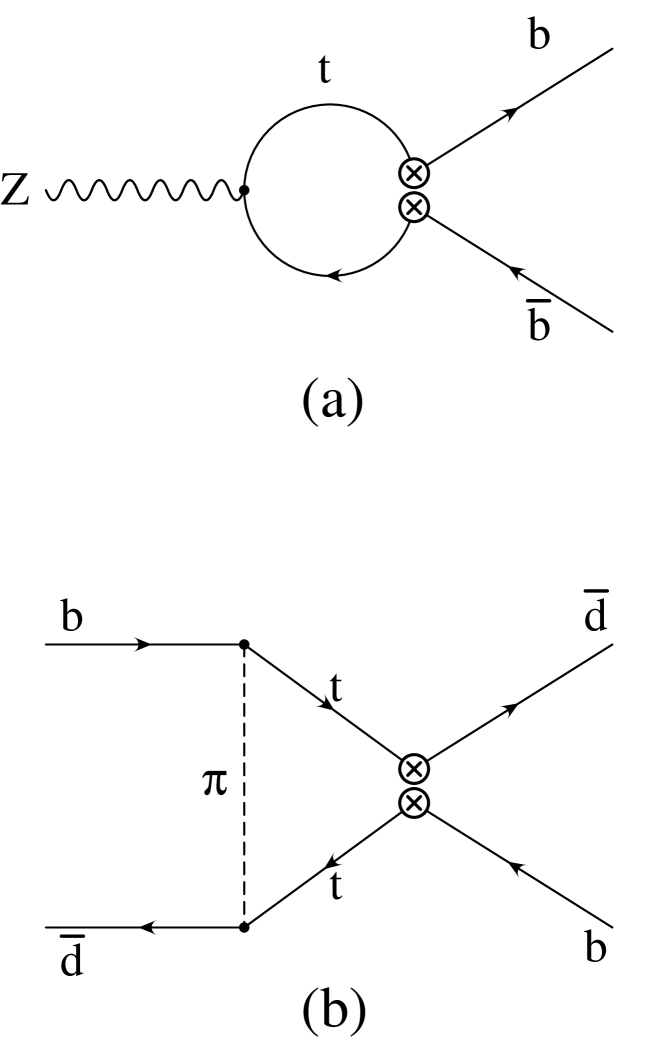
Figure 1: a) Contribution of the effective operator $O_{11}$ to $Z\rightarrow b\bar{b}$. b) Contribution of the effective operator $O_{11}$ to $B$–$\bar{B}$ mixing

References

• [1] T. Appelquist, β€œGauge Theories and Experiments at High Energies”, ed. K.C. Brower and D.G. Sutherland (Scottish University Summer School in Physics, St. Andrews); T. Appelquist and C. Bernard, Phys. Rev. D22, 200 (1980)
• [2] A.C. Longhitano, Phys. Rev. D22, 1166 (1980); Nucl. Phys. B188, 188 (1981)
• [3] M.E. Peskin and T. Takeuchi, Phys. Rev. Lett. 65, 964 (1990); Phys. Rev. D46, 381 (1992); W. Marciano and J. Rosner, Phys. Rev. Lett 65, 2963 (1990)
• [4] G. Altarelli and R. Barbieri, Phys. Lett. B253, 161 (1990); G. Altarelli, R. Barbieri and J.Β Jadach, Nucl. Phys. B369, 3 (1992)
• [5] See for instance F. Feruglio, Int. J. Mod. Phys. A8, 4937 (1993)
• [6] J. Bernabeu, D. Comelli, A.Β Pich and A.Β Santamaria in preparation.
• [7] I. Tomalin, β€œRbsubscript𝑅𝑏R_{b} with Multivariate Analysis”, talk at the ICHEP 96 Conference, Warsaw, July 1996.
• [8] The LEP Electroweak Working Group and the SLD Heavy Flavor Group, β€œA Combination of Preliminary LEP and SLD Electroweak Measurements and Constraints on the Standard Model”. Report LEPEWWG/96-02, 1996.
• [9] A.Β Akundov, D.Β Bardin and T.Β Riemann, Nucl.Β Phys. B276, 1 (1986); J.Β BernabΓ©u, A.Β Pich, and A.Β Santamaria, Phys.Β Lett. B200, 569 (1988); Nucl. Phys. B363, 326 (1991); W.Β Beenakker and W.Β Hollik, Z.Β Phys. C40, 141 (1988)
• [10] G. Buchalla, A.J. Buras and M.E. Lautenbacher, β€œWeak Decays Beyond Leading Logarithms” Submitted to Rev. Mod. Phys. [hep-ph/9512380].
• [11] L. Gibbons, Quark Masses and Mixing from Weak Processes, Plenary talk at the $28^{\mbox{\rm\scriptsize th}}$ International Conference on High Energy Physics (Warsaw, 1996)
• [12] L. Wolfenstein, Phys. Rev. Lett. 51, 1945 (1983)
• [13] A.J. Buras, Flavour Changing Neutral Current Processes, Plenary talk at the $28^{\mbox{\rm\scriptsize th}}$ International Conference on High Energy Physics (Warsaw, 1996), [hep-ph/9610461].
• [14] A. Pich and J. Prades, Phys.Β Lett. B346, 342 (1995);
• [15] A.J. Buras, M. Jamin and P.H. Weisz, Nucl. Phys. B347, 491 (1990)
Refer to caption