Factorization for hard exclusive electroproduction of mesons in QCD

Abstract

We formulate and prove a QCD factorization theorem for hard exclusive electroproduction of mesons in QCD. The proof is valid for the leading power in $Q$ and all logarithms. This generalizes previous work on vector meson production in the diffractive region of small $x$. The amplitude is expressed in terms of off-diagonal generalizations of the usual parton densities. The full theorem applies to all kinds of meson and not just to vector mesons. The parton densities used include not only the ordinary parton density, but also the helicity density ($g_{1}$ or $\Delta q$) and the transversity density ($h_{1}$ or $\delta q$), and these can be probed by measuring the polarization of the produced mesons with unpolarized protons.

I Introduction

In two recent papers [1, 2] it was shown how the cross section for diffractive electroproduction of vector mesons can be predicted in perturbative QCD. This process provides a novel probe of the dynamics of diffractive scattering in QCD. One notable prediction is that the cross section is proportional to the square of the gluon density in the hadron. Experimental data [4, 5, 6] appear to be in accord with the predictions, including an enhancement due to the rapid rise of the gluon density at small $x$.

In this paper we extend the factorization theorem to the general case of electroproduction of any meson, and we provide a general proof of the theorem. The theorem expresses the amplitude for the process in terms of off-diagonal generalizations of the usual parton densities. Our demonstration is valid for the whole leading power for the process, in contrast with the calculations in Ref. [1, 2], which were in a leading-logarithm approximation. Our results will enable the process to be treated with the inclusion of non-leading logarithms. Apart from establishing the factorization theorem for the process, one aim of this paper is to attempt a pedagogical exposition of the methods by which the theorem is derived, since many of the concepts are unfamiliar.

Most importantly, the process of constructing a proof led us to new results. First, the theorem applies to the general case of two-body final states at low transverse momentum in electroproduction at large $Q$. The diffractive case simply corresponds to the small-$x$ region, with vacuum quantum number exchange. So we have extended the theorem to the full range of $x$ and to all mesons, pions in particular, not just vector mesons. In addition we find that we need not only the usual unpolarized parton densities (generalized to be off-diagonal), but also the helicity densities ($g_{1}$ or $\Delta q$) and the transversity densities ($h_{1}$ or $\delta q$). Since the cross section is proportional to the square of the densities, it is sensitive to the polarized parton densities without needing a polarized proton beam and without needing a measurement of the polarization of the final-state proton. Indeed we can choose which kind of density is probed merely by choosing the final state meson. The amplitude for longitudinally polarized vector mesons depends only on the unpolarized parton densities. The amplitude for transversely polarized vector mesons depends only on the transversity densities ($h_{1}$). The amplitude for pseudoscalar mesons depends only on the helicity densities.

This result clearly adds to the meager list of processes where the transversity of valence quarks can be probed without the need of some other unknown quantity (such as an antiquark density or a polarized fragmentation function).

All the above statements apply when the incoming virtual photon is longitudinally polarized. We also prove that the cross section is suppressed by a power of $Q$ when the photon is transversely polarized.

We give a fairly detailed account of the proof of the factorization theorem. The style of proof is based on that of Refs. [8, 9, 10, 11], which treat inclusive hard scattering. There are some differences. First, our derivation of the power-counting formula shows some useful improvements. Secondly, and rather importantly, we have to examine more closely exchanges of relatively soft quarks, since, in contrast to the case of inclusive scattering, there can be leading contributions from soft quark exchange (otherwise known as the endpoint contributions). Thus we have to examine the power-counting arguments in more detail.

After this work was substantially complete, Radyushkin [12] published a preprint treating some of the same processes that we consider. His work appears to be completely compatible with ours; he takes the same point of view as we do concerning a generalized operator product expansion, although the details of his notation are a little different. However, he considered only the diffractive limit of small $x$ for vector meson production, and hence, just as in Ref. [1], he did not include the quark contribution. (The quark operator is presumably unimportant at small $x$.) He does not present a complete proof of factorization. Ji [13] and Radyushkin [14] also showed how the same operators appear in an expansion for deeply virtual Compton scattering.

In a future paper we hope to explore further consequences of our results, including detailed calculations.

II Definition of process

The process we treat is the diffractive exclusive production of mesons in deep-inelastic electroproduction. We can express the lepto-production cross section in terms of the cross section for the scattering of virtual photons:

$$\gamma^{*}(q)+p\to V(q+\Delta)+p^{\prime}(p-\Delta).$$ (1)

The target, of momentum $p^{\mu}$, can be a proton or nucleus (or any other hadron), and the diffracted hadron $p^{\prime}$, of momentum $p-\Delta$, may or may not have the same flavor quantum numbers as the incoming hadron $p$. The other final-state particle, $V$, can be any possible meson, e.g., $\rho^{0}$, $\omega$, $J/\psi$, $\Upsilon$ or $\pi$. When we treat charge exchange scattering within our framework, the direct connection to the parton densities in the proton [1, 2, 3, 7] is lost. We will assume that the meson has quantum numbers such that it cannot decay to a gluon pair. This choice will eliminate certain subprocesses, and covers the mesons of interest.

The process depends on three kinematic variables: the virtual photon’s virtuality, $Q^{2}\equiv-q^{2}$, the square of the center-of-mass energy, $s$ (for the photon-proton system), and the momentum transfer squared, $t=\Delta^{2}\leq 0$. The region we consider is where $Q^{2}\gg\Lambda^{2}_{\rm QCD}$, while $|\Delta^{2}|$ is small, of order $\Lambda^{2}_{\rm QCD}$. We also assume that the meson mass obeys $m_{V}^{2}\ll s$. We are thus treating the asymptotics as $Q$ gets large. The Bjorken variable is $x=Q^{2}/2p\cdot q\approx Q^{2}/(s+Q^{2})$ (where the target mass is neglected). In Refs. [1, 2] the diffractive case $x\ll 1$ was treated. Our considerations will apply to large $x$ as well.

We will mostly restrict our attention to the case that the virtual photon is longitudinally polarized. The cross section with transversely polarized photons is somewhat smaller — this was a prediction of Refs. [1, 2], and is confirmed experimentally, although the suppression is not as much as one might expect. Indeed, we find we can derive a simple factorization theorem only for longitudinally polarized photons, since then the contributions from the endpoints $z\to 0$ and $z\to 1$ of the meson wave function are power suppressed, given that the meson wave function at its endpoints behaves approximately as $z(1-z)$. For transverse polarization, this suppression does not happen, and a more complicated theorem is needed—see Sec. X. At high enough $Q$, there is a Sudakov suppression, but the physics of this goes beyond the simple factorization theorem, just as in the analogous case of the electromagnetic form factor of the proton [16].

It is convenient to use light-front coordinates defined with respect to the collision axis: $v^{\mu}=(v^{+},v^{-},v_{\perp})$, with $v^{\pm}=(v^{0}\pm v^{3})/\sqrt{2}$. Then we can write

$$p^{\mu} = \left(p^{+},\frac{m^{2}}{2p^{+}},{\bf 0}_{\perp}\right),$$ (2)

$$q^{\mu} \approx \left(-xp^{+},\frac{Q^{2}}{2xp^{+}},{\bf 0}_{\perp}\right),$$ (3)

$$\Delta^{\mu} \approx \left(xp^{+},-\frac{\Delta_{\perp}^{2}+m^{2}x}{2(1-x)p^{+}},{\bf\Delta}_{\perp}\right),$$ (4)

$$V^{\mu} \approx \left(\frac{\Delta_{\perp}^{2}+m_{V}^{2}}{Q^{2}}xp^{+},\frac{Q^{2}}{2xp^{+}},{\bf\Delta}_{\perp}\right).$$ (5)

Here, $V^{\mu}$ is the momentum of the meson. In these equations, we have neglected small terms in the longitudinal components, of relative size $\Lambda_{\rm QCD}^{2}/Q^{2}$. These coordinates agree with the ones used in Refs. [8, 11], but differ from those in Refs. [1, 2] by a factor of $\sqrt{2}$, and by a change of the use of the $+$ and $-$ labels: $v^{+}_{\rm this\ paper}={v_{-}}_{\rm Ref.\ \cite[cite]{[\@@bibref{Number}{BFGMS}{}{}]}}/\sqrt{2}$, and similarly for $v^{-}$.

III Statement of theorem

A Theorem

The theorem we will prove is that the amplitude for the process Eq. (1) is [1]

$${\cal M} = \sum_{i,j}\int_{0}^{1}dz\int dx_{1}f_{i/p}(x_{1},x_{1}-x,t,\mu)\,H_{ij}(Q^{2}x_{1}/x,Q^{2},z,\mu)\,\phi^{V}_{j}(z,\mu)$$ (7)

$$+\mbox{power-suppressed corrections}.$$

Here, $f_{i/p}$ is just like the distribution function for partons of type $i$ in hadron $p$, except that it is a non-forward matrix element. We will give the definition later. The factor $\phi^{V}_{j}$ is the light-cone wave function for the meson, and $H_{ij}$ is the hard scattering function. The sums are over the parton types $i$ and $j$ that connect the hard scattering to the distribution function and to the meson. Since the meson has non-zero flavor, the parton $j$ is restricted to be a quark. The factorization theorem Eq. (7) is illustrated in Fig. 1.

The above formula is correct for the production of longitudinally polarized vector mesons. For the production of transversely polarized vector mesons or of pseudo-scalar mesons, we have a formula of exactly the same structure, but in which the unpolarized parton density is replaced by a polarized parton density (the transversity density for transverse vector mesons, and the helicity density for pseudo-scalar mesons). Similar changes will need to be made to the definition of the meson wave function.

FIG. 1.: Factorization theorem.

The parameter $\mu$ in Eq. (7) is the usual renormalization/factorization scale. It should be of order $Q$, in order that the hard scattering function $H_{ij}$ be calculable by the use of finite-order perturbation theory. The $\mu$-dependence of the distribution $f_{i/p}$ and of the light-cone wave function $\phi_{j}^{V}$ are given by equations of the Dokshitzer-Gribov-Lipatov-Altarelli-Parisi (DGLAP) kind, as we will discuss in Sec. VIII.

Typical lowest order graphs for $H$ are shown in Fig. 2. Consider first graph (a), all of whose external lines are quarks. After we go through the derivation of the factorization theorem, and have constructed definitions of the distribution $f_{i/p}$ and of the light-cone wave function $\phi^{V}$, we will be able to see that the definition of $H$ is the sum of graphs such as Fig. 2(a) contracted with suitable external line factors that correspond to the Dirac wave functions of the partons. In the case of longitudinal vector meson production, the factors are $\frac{1}{2}p^{+}\gamma^{-}$ for the lower two lines and $\frac{1}{2}V^{-}\gamma^{+}$ for the lines connected to the outgoing meson. These factors are related to spin averages of Dirac wave functions for the quarks.

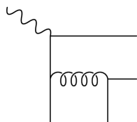
(a)	(b)

FIG. 2.: Typical lowest-order graphs for $H$.

In the case of the gluon-induced subprocess, Fig. 2(b), the external fermion lines of $H$ are to be contracted with the same factors as before, but the two gluon lines are to be contracted with $\delta^{\alpha\beta}/2$, where $\alpha$ and $\beta$ are transverse indices, and the $1/2$ represents a kind of spin average.

See Sec. IX for more information on the precise normalization conventions for the hard scattering function.

B Definitions of light-cone distributions and amplitudes: longitudinal vector meson

1 Quark distribution

The distribution function $f_{i/p}$ and meson amplitude $\phi^{V}_{j}$ are defined, as usual, as matrix elements of gauge-invariant bilocal operators on the light-cone. In the case of a quark of flavor $i$, we define

$$f_{i/p}(x_{1},x_{2},t,\mu) = \int_{-\infty}^{\infty}\frac{dy^{-}}{4\pi}\;e^{-ix_{2}p^{+}y^{-}}\langle p^{\prime}|\;T{\bar{\psi}}(0,y^{-},{\bf 0}_{T})\gamma^{+}{\cal P}\psi(0)\;|p\rangle,$$ (8)

where $\cal P$ is a path-ordered exponential of the gluon field along the light-like line joining the two operators for a quark of flavor $i$. We have defined $x_{1}$ to be the fractional momentum given by the quark to the hard scattering and $-x_{2}$ to be the momentum given by the antiquark; in the factorization theorem they obey $x_{1}-x_{2}=x$, with $x$ being the usual Bjorken variable. At first sight the right-hand-side of Eq. (8) appears to depend only on $x_{2}$ and not on $x_{1}$ nor on $t$. The dependence on the other two variables comes from the fact that the matrix element is non-forward. The difference in momentum between the states $|p\rangle$ and $|p^{\prime}\rangle$ together with the use of a light-cone operator brings in dependence on $x_{1}$ and on $t$. It is necessary to take only the connected part of the matrix element.

The same definition has recently been given and discussed by Ji and Radyushkin [12, 13, 14]. As Ji points out, when $t\not=0$ there are in fact two separate parton densities, with different dependence on the nucleon spin. For the purposes of our proof, it will be unnecessary to take this into account explicitly; we can simply suppose that this and the other parton densities have dependence on the spin state of the hadron states $|p\rangle$ and $|p^{\prime}\rangle$.

The usual quark density $f_{i/p}(x,\mu)$ is obtained by setting $t=0$ and $x_{1}=x_{2}=x$ in Eq. (8). In addition, it would appear that one has to remove the time-ordering operation from the operator operators in Eq. (8) to obtain the operator used for the parton densities associated with inclusive scattering [17]. We need time-ordered operators in our present work because we are discussing amplitudes rather than cut amplitudes. Thus if one sets $t=0$ and $x_{1}=x_{2}=x$ in our parton distributions, one would naturally suppose that the conventional inclusive parton densities are the discontinuities of ours. Relating the new parton densities to the standard ones, even in the forward limit would therefore appear to need dispersion relations.

In fact, the two kinds of parton density are equal, at least in the forward limit. A proof of this not very obvious fact was given many years ago by Jaffe [18]. However, his proof applies only to two-particle-irreducible graphs for the parton densities, a restriction we suspect to be unnecessary. We hope to return to this issue in a later paper, particularly because there are some additional complications in the non-forward parton densities that particularly appear when one treats dispersion relations for the amplitude for our process.

It is also worth noting that there is a limit on $t$:

$$-t>t_{\rm min}=\frac{m^{2}(x_{1}-x_{2})^{2}}{1-x_{1}+x_{2}},$$ (9)

which comes from the kinematics of the scattering proton. Note that the same limit is obtained from the kinematics of the scattering process we consider, (1), in the limit $Q\gg m$. We deduce that the limit $t\to 0$ cannot be accessed directly in exclusive meson production. Indeed, since $x_{1}-x_{2}=x_{\rm bj}$, the analytic continuation from $t\not=0$ to $t=0$ is hard to perform in practice, except at small $x_{\rm bj}$.

2 Gluon distribution

An exactly similar definition applies for the gluon distribution:

$$f_{g/p}(x_{1},x_{2},t,\mu) = -\int_{-\infty}^{\infty}\frac{dy^{-}}{2\pi}\,\frac{1}{x_{1}x_{2}p^{+}}\;e^{-ix_{2}p^{+}y^{-}}\langle p^{\prime}|\;TG_{\nu}{}^{+}(0,y^{-},{\bf 0}_{T})\,{\cal P}\,G^{\nu+}(0)\;|p\rangle.$$ (10)

The $1/x_{1}x_{2}$ factor cancels a inverse factor that appears in the derivative part of the fields $G_{\nu}{}^{+}(0,y^{-},{\bf 0}_{T})G^{\nu+}(0)$. The normalization is now a little different from that of the diagonal distribution:

$$f_{g~{}\rm diag}(x)=xf_{g~{}\rm non-diag}(x,x),$$ (11)

i.e., one sets $x_{1}=x_{2}=x$, and puts in a factor $x$. To avoid this complication while preserving symmetry between the two gluon lines would involve square root factors, or changing the hard scattering formula Eq. (7) when the partons are gluons. The square roots are undesirable, because they change the analyticity properties of the formula in the neighborhood of $x_{1}=0$ and $x_{2}=0$.

3 Wave function

The light-cone wave function for a longitudinally polarized vector meson is [19]

$$\phi^{V}_{j}(z,\mu^{2}) = \frac{1}{\sqrt{2N_{c}}}\int_{-\infty}^{\infty}\frac{dy^{+}}{4\pi}\;e^{-izV^{-}y^{+}}\langle 0|\;{\bar{\psi}}(y^{+},0,{\bf 0}_{T})\gamma^{-}{\cal P}\psi(0)\;|V\rangle,$$ (12)

where the factor of $1/\sqrt{2N_{c}}$ is the convention established by Brodsky and Lepage [20]—see their Eq. (64). This convention results in a elegant normalization condition for light-cone wave functions, Eq. (26) of Ref. [20].

Our definition appears to disagree with theirs, but this is fact not so. We have an extra overall factor $2$ which merely results from the $1/\sqrt{2}$’s in our definition of light-cone coordinates. We are missing a $\gamma_{5}$ that they have, because our meson is a vector instead of a pseudoscalar, and we therefore need a different operator to pick out the nonzero component. In addition, we have exchanged the use of the $+$ and $-$ components of vectors. This simply corresponds to the fact that we wish to apply the definition to a meson that travels in the $-z$ direction in our coordinate system. The factor of $P_{\pi}^{+}$ in Brodsky and Lepage’s definition is an error, and should be omitted [21]: their definition is not invariant under boosts in the $z$ direction.

All of the above definitions have ultra-violet divergences. So they are defined [17] to be renormalized by some suitable prescription, of which minimal subtraction is the standard one. We do not explicitly indicate the renormalization, which is done by a factor convoluted with the right-hand sides of these definitions. The scale associated with the renormalization is $\mu$, and the DGLAP evolution equations are the renormalization-group equations for the $\mu$ dependence.

As stated in footnote § ‣ III A, there is a more general theorem, in which the final-state hadron in the distribution Eq. (8) has quantum numbers different from the proton. Then it would be necessary to modify this definition, so that the quark and antiquark fields have different flavors. (The gluon distribution would also be zero.) Similar modifications would be needed to the meson amplitude Eq. (12).

C Definitions of light-cone distributions and amplitudes: pseudo-scalar meson and transverse vector meson

When we write the factorization formula for a pseudo-scalar meson, different components components of Dirac matrices dominate in the amplitudes. We will see that the following changes are needed in the definitions, Eqs. (8), (10) and (12):

Object original replacement (pseudo-scalar meson)

Meson wave function $$\gamma^{-}$$

Quark density

Gluon density Not used

Coupling of to quarks from meson

Coupling of to quarks from proton

Coupling of to gluons from proton Not used

(13)

The parton densities in the diagonal limit then correspond to the helicity densities [22] $\Delta f$ that are used in the treatment of the polarized structure function $g_{1}$. However, the gluon density is not used: charge conjugation invariance implies that the hard scattering coefficient is zero when it couples a virtual photon and a pseudo-scalar meson to a pair of gluons.

For a transversely polarized vector meson, we use the following replacements

Object original replacement (transverse vector meson)

Meson wave function $$\gamma^{-}$$

Quark density

Gluon density Not used

Coupling of to quarks from meson

Coupling of to quarks from proton

Coupling of to gluons from proton Zero

(14)

Note that the gluon density does not appear in this case, for reasons of helicity conservation in the hard scattering. In the diagonal limit, the quark density we use with transversely polarized vector mesons becomes the transversity density [22] $\delta f_{q}$, also called $h_{1}$.

The combinations of Dirac matrices in the wave functions for longitudinal vector mesons and pseudo-scalar mesons pick out pairs quark and antiquarks that have opposite helicity and hence of the chirality; this is correct for making a meson of zero helicity. In contrast for a transverse vector meson, the quark and antiquark have the same helicities and the opposite chiralities.

D Real and imaginary parts of amplitude

In the factorization theorem, Eq. (7), the amplitude for our process at the hadronic level is expressed in terms of a hard scattering amplitude together with a generalized parton density in the proton and a light-cone wave function of the meson. Now both the hadronic amplitude and the hard scattering amplitude satisfy dispersion relations that relate their real and imaginary parts, and it is not entirely obvious that the dispersion relations for the two amplitudes are consistent with the factorization theorem. Moreover, one might suppose that complications arise because the cut of the amplitude needed to obtain the discontinuity of the hadronic amplitude must cut both the hard scattering amplitude and the parton density in Fig. 1.

We now demonstrate that the two dispersion relations are in fact consistent. The proof will be to demonstrate that the dispersion relation for the hadronic amplitude follows from the corresponding dispersion relation for the hard scattering amplitude. This is important because one of the approaches to calculations has been to calculate the imaginary part of the amplitude first and then to use dispersion relations to compute the full amplitude. A consequence is that the real and imaginary parts of the hadronic amplitude are separately expressed in terms of the real and imaginary parts of the hard scattering amplitude with the same parton densities.

We will find it convenient to write the amplitude as a function of $\nu\equiv 2p\cdot q=Q^{2}/x$ rather than $s=\nu-Q^{2}$. We have ${\cal M}={\cal M}(Q^{2}/x,t,Q^{2})$ and $H=H(Q^{2}x_{1}/x,Q^{2},z)$, where $x_{1}$ is the same variable as in Eq. (7). The important fact that lets our derivation work is that $H$ depends on the ratio $x_{1}/x$ but not on $x_{1}$ and $x$ separately. This is proved by observing that $H$ is invariant under Lorentz boosts in the $z$ direction and that a change of $x_{1}$ and $x$ by a common ratio is equivalent to a boost.

The dispersion relation for the hard scattering amplitude is

$$H(\nu,Q^{2},z) = \int\frac{d\nu^{\prime}}{2\pi i}\frac{1}{\nu^{\prime}-\nu}{\rm disc}\,H(\nu^{\prime},Q^{2},z).$$ (15)

By choosing the contour to run along the real axis, we have made the right-hand side of this equation involve only the discontinuity (or imaginary part) of the amplitude. Any subtractions needed in the dispersion relation will not affect the principles of the derivation.

We now substitute Eq. (15) in the factorization theorem. Then writing $\nu^{\prime}=x_{1}\hat{\nu}$ gives the dispersion relation for $\cal M$:

$${\cal M}(\nu,Q^{2},t) = \int dx_{1}dz\frac{d\nu^{\prime}}{2\pi i}\frac{1}{\nu^{\prime}-\nu x_{1}}H(\nu^{\prime},Q^{2},z)\phi(z)f(x_{1},x^{\prime}).\$$ (16)

$$= \int dx_{1}dz\frac{d\hat{\nu}}{2\pi i}\frac{1}{\hat{\nu}-\nu}H(x_{1}\hat{\nu},Q^{2},z)\phi(z)f(x_{1},x^{\prime}).$$ (17)

$$= \int\frac{d\hat{\nu}}{2\pi i}\frac{1}{\hat{\nu}-\nu}{\rm disc}\,{\cal M}(\hat{\nu},Q^{2},z),$$ (18)

where in the last line, we have used the factorization theorem again. This equation is just the expected dispersion relation for the hadronic amplitude.

The discontinuity of an amplitude is obtained by making a cut that puts some intermediate states on shell. The only possible cut of $\cal M$ in its factorized form Fig. 1 is one that cuts both the hard scattering amplitude $H$ and the parton density $f$. The statement that the parton densities are the same whether the operators are unordered or are time-ordered is equivalent to saying that the cut amplitude equals the uncut amplitude. This is consistent with our derivation of the dispersion relation for $\cal M$.

IV Regions

We wish to calculate the asymptotics in a double limit: $Q/m\to\infty$ and $x\to 0$, but it is the $Q\to\infty$ limit that we will concentrate on, since that will result in the perturbatively calculable factors in our theorem. It will also give us a more general theorem, that is applicable at large $x$. In this and the next section we follow the treatment of Libby and Sterman [10, 23, 24] adapted to our process.

Graphs for the process have integrals over all their loop momenta, and we wish to classify the regions of loop momenta in a suitable way for extracting the asymptotics as $Q\to\infty$. To expose the powers of $Q$, we choose to work in the Breit frame where the virtual photon has zero rapidity, $xp^{+}=Q^{2}/2xp^{+}=Q/\sqrt{2}$. In such a frame the meson $V$ is moving very fast in one direction, and the incoming and outgoing protons are moving very fast in the opposite direction. The steps in the proof are as follows:

1. Scale all momenta by a factor $Q/m$, so that we are in effect attempting to take a massless on-shell limit of the amplitude.

2. Use the Coleman-Norton theorem to locate all pinch-singular surfaces in the space of loop integration momenta, in the zero-mass limit.

3. Identify the relevant regions of integration as neighborhoods of these pinch singular surfaces.

4. The scattering amplitude is a sum of contributions, one for each pinch singular surface, plus a term where all lines have virtuality of at least of order $Q^{2}$. Appropriate subtractions are made to prevent double counting.

5. Perform power counting to determine which regions give the largest power of $Q$.

6. Finally, show that the contributions for the leading power of $Q$ give the factorization formula Eq. (7).

Any terms that do not contribute to the leading power are dropped. The factorization formula is intended to include all logarithmic corrections to the leading power, whether they are leading or non-leading logarithms.

A Scaling of momenta

Following Libby and Sterman[23] we write a general momentum $k^{\mu}$ and a general mass $m$ in units of the large momentum scale $Q$:

$$k^{\mu}=Q\tilde{k}^{\mu},~{}~{}~{}m=Q\tilde{m}.$$ (19)

Since we work in the rest frame of the virtual photon, i.e., in the Breit frame, both of the light-cone components of its momentum are of order $Q$. When everything is expressed in terms of the scaled variables, $\tilde{k}$ and $\tilde{m}$, simple dimensional analysis shows that the large-$Q$ limit is equivalent to a zero-mass limit, $\tilde{m}\to 0$. Since the amplitude $\cal M$ is dimensionless, we have

$${\cal M}(Q^{2};p,p_{V},\Delta,m;\mu)={\cal M}(1;\tilde{p},\tilde{p}_{V},\tilde{\Delta},\tilde{m};\mu/Q),$$ (20)

by ordinary dimensional analysis. Notice that in the limit $Q\to\infty$

$$\tilde{p}^{\mu} \to (p^{+}/Q,0,{\bf 0}_{\perp}),$$ (21)

$$\tilde{q}^{\mu} \to (-xp^{+}/Q,Q/(2xp^{+}),{\bf 0}_{\perp}),$$ (22)

$$\tilde{\Delta}^{\mu} \to 0,$$ (23)

$$\tilde{V}^{\mu} \to (0,Q/(2xp^{+}),{\bf 0}_{\perp}),$$ (24)

so that $\tilde{p}$ and $\tilde{V}$ become light-like vectors, cf. Eq. (5).

We consider the most basic region to be where all internal lines obey $k^{2}\gtrsim Q^{2}$, and thus the scaled momenta $\tilde{k}$ have virtualities of order unity, or bigger. In such a region, we can legitimately set the mass parameters to zero, and make the external hadrons light-like. Most importantly, we will be entitled to choose the renormalization scale $\mu$ of order $Q$ without obtaining any large logarithms. Consequently, in this region an expansion to low order in powers of the small coupling $\alpha_{s}(Q)$ is useful.

However, this basic region is not the only one. Indeed, it does not even provide a leading contribution for the amplitude for our particular process. But now one observes [23] that all other relevant regions correspond to singularities of massless Feynman graphs. They are neighborhoods of surfaces where the loop momenta are trapped at singularities, i.e., of pinch-singular surfaces of the massless graphs. The conditions for a pinch singularity are exactly the Landau conditions for a singularity of a graph. Only pinch singularities are relevant, since at a non-pinched singularity, we may deform the (multi-dimensional) integration contour such that at least one of the singular propagators is no longer near its pole.

If there is a pinch singularity caused by certain propagator poles in the massless limit, then in the real graph, with nonzero masses but large $Q$, the contour of integration is forced to pass near the propagator poles. Consequently it is not possible to neglect the masses in this region. Conversely, if the contour is not trapped by the poles, then the contour may be deformed away from the poles, and masses may be neglected in evaluating the corresponding propagators.

B Coleman-Norton theorem

We now review the theorem of Coleman and Norton [25], and show how [24] to apply it. The theorem shows in a physically appealing fashion how to determine the configurations of loop momenta that give pinch singularities; it states that they correspond to classically allowed scattering processes, treated in coordinate space.

More precisely, the theorem states that each point on a pinch-singular surface (in loop momentum space) corresponds to a space-time diagram obtained as follows. First we obtain a reduced graph by contracting to points all of the lines whose denominators are not pinched. Then we assign space-time points to each vertex of the reduced graph in such a way that the pinched lines correspond to classical particles. That is, to each line we assign a particle propagating between the space-time points corresponding to the vertices at its ends. The momentum of the particle is exactly the momentum carried by the line, correctly oriented to have positive energy. If for some set of momenta, it is not possible to construct such a reduced graph, then we are free to deform the contour of integration.

A reduced diagram corresponds to a classically allowed space-time scattering process. The construction of the most general reduced graph becomes extremely simple in the zero mass limit, since then all pinched lines must carry either a light-like momentum or zero momentum. Moreover, as was explained by Libby and Sterman, each light-like momentum must be parallel to one of the (light-like) external lines.

C Reduced graphs

In the zero mass limit, our process, represented in Fig. 3, has

• One light-like incoming proton line of momentum $p_{A}^{\mu}=(p^{+},0,0_{\perp})$.

• One light-like outgoing proton line of a slightly different, but parallel, momentum
  $p_{A}^{\prime\mu}=((1-x)p^{+},0,0_{\perp})$.

• One light-like outgoing meson line of momentum $p_{B}^{\mu}=(0,Q^{2}/2xp^{+},0_{\perp})$.

• One incoming virtual photon of momentum $q^{\mu}=(-xp^{+},Q^{2}/2xp^{+},0_{\perp})$.

We have chosen the symbols for the light-like momenta, $p_{A}$, $p_{A}^{\prime}$, and $p_{B}$, to be different from the symbols for the corresponding physical momenta, $p$, $p^{\prime}$, and $V$, precisely to emphasize that they are distinct (if related) momenta.

FIG. 3.: Quasi-elastic scattering of a virtual photon on a proton.

FIG. 4.: General reduced graph for Fig. 3. The dots represent the possibility of an arbitrary number of lines connecting the collinear subgraphs ($A$ and $B$) to the hard subgraph $H$. Any number of lines connect the soft subgraph $S$ to the other subgraphs.

As we will prove in Sec. IV F, the most general reduced graph is depicted in Fig. 4. One vertex of the reduced graph is the hard subgraph $H$, to which is attached the virtual photon. The incoming and outgoing protons go into the collinear subgraph $A$; at the corresponding pinched momentum configuration, lines in $A$ have only a $+$ component. Similarly, the outgoing meson is attached to another collinear subgraph $B$ where there are momenta with only a $-$ component. Each of the collinear subgraphs is attached to the hard subgraph by at least one line, and these three subgraphs are all connected; these restrictions are needed so that momentum conservation works out. Finally there may be a soft subgraph, $S$, composed of zero momentum lines at the pinch singular surface. It connects to any of the other subgraphs, and it may have more than one connected component.

Within any of $A$, $B$ and $S$, there may be subgraphs composed of hard lines; these form reduced vertices that couple the different lines within the subgraphs. In the leading regions, these are of the form of the possible ultra-violet divergent subgraphs.

D Space-time interpretation

The corresponding space-time diagram is Fig. 5. There, each solid line corresponds to a light-like line of the reduced graph, with a $45^{\circ}$ orientation to correspond to their light-like lines of propagation. The dashed lines correspond to the soft lines, in the subgraph $S$. From the point of view of the Coleman-Norton theorem, they are rather degenerate lines. Indeed, the fact that they are carrying zero-momentum (at the singular point) implies that they have no specific orientation. Thus we indicate them by curved lines of no particular orientation. The locations of the endpoints of the soft lines, where they attach to the collinear subgraphs, can be anywhere along the world lines of the collinear lines. The hard vertex $H$ occurs at the intersection of the collinear lines.

Since there can in general be more than one collinear line moving in each of the $+$ and $-$ directions, the solid lines in Fig. 5 must each be thought of as a group of lines which undergo interactions as they propagate.

FIG. 5.: Space-time diagram for Fig. 4.

When the space-time representation of a Feynman graph is used, there is normally an exponential suppression when there are large space-time separations between the vertices. One obtains a singularity when the exponential suppression fails, and the Coleman-Norton construction gives exactly the relevant configurations of the vertices. A common scaling can be applied to all the world lines in the reduced graph without affecting its properties, and the singularity is generated by the possibility of integrating over arbitrarily large scalings in coordinate space without obtaining an exponential suppression.

The whole of the discussion above relies on the use of a covariant gauge. Although the use of the axial gauge and in particular of the light-cone gauge is very convenient, for example, for a physical interpretation of the light-cone wave function, the propagators in such a gauge have unphysical singularities. The unphysical singularities do not give the normal rules of causal relativistic propagation of particles, and, beyond the leading-logarithm approximation, they make the derivation of the factorization theorem very difficult — see [8, 26].

E Examples

To understand what Fig. 5 means, let us look at a few examples of regions of momentum space that correspond to reduced graphs obtained from the Feynman graph of Fig. 6(a). There the couplings between the quarks and the hadrons may be considered as Bethe-Salpeter wave functions. We will not give an exhaustive list of all possible reduced graphs, but will only give some typical examples that correspond to leading power contributions to the amplitude.

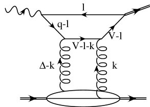
(a)	(b)
(c)	(d)

FIG. 6.: A low order graph for diffractive meson production, together with three of its reduced graphs. The solid lines are meant to be at a $45^{\circ}$ angle to represent light-like propagation, but have been separated to permit the structure to be seen.

1 First example

We first consider a region defined as follows: The upper two loops have momenta

$$k \sim \left(x_{1}p^{+},O(m^{2}/xp^{+}),O(m)\right),$$ (25)

$$l \sim \left(O(m^{2}/Q),zQ^{2}/2xp^{+},O(m)\right).$$ (26)

where $m$ represents a typical hadronic scale. We continue to use a coordinate system like the Breit frame where $xp^{+}\sim Q$, and we label the components in the order $(+,-,\perp)$. The parameter $z$, for the $-$ component of $l$ lies between 0 and 1, and is not close to its endpoints. The parameter $x_{1}$, for the $+$ component of $k$ is chosen such that both $x_{1}$ and $x-x_{1}$ are of order $x$ and are both positive. Finally, the region is such that all the lower three lines have momentum components of size $\left(O(p^{+}),O(m^{2}/p^{+}),O(m)\right)$.

Another way of defining the region is to say that the quark lines $l$ and $V-l$ are collinear to $V$, the quark lines $q-l$ and $V-l-k$ are hard, and all the remaining lines are collinear to $p$.

This region forms a neighborhood of the configuration defined by the reduced diagram in Fig. 6(b). In this configuration, the lines of momenta $q-l$ and $V-l-k$ form the hard vertex, since they have virtuality of order $Q^{2}$. The lower 3 quark lines, and the two gluons have momenta proportional to $(p^{+},0,0_{\perp})$, while the lines $l$ and $V-l$ have momenta proportional to $(0,Q^{2}/p^{+},0_{\perp})$. In the reduced diagram, the light-like momenta are represented by lines in approximately the $45^{\circ}$ directions that represent their world lines. Since both of $k$ and $\Delta-k$ have positive $+$ momenta, they are forward moving lines.

It is important to make a pedantically exact distinction between the momentum configuration represented by the reduced graph and the region of integration that we attach to it. Confusion between the two concepts results in misunderstanding of the content of parton-model concepts. The configuration contains a collection of light-like momenta derived by certain rules, while the region is a neighborhood of this configuration. The graph, Fig. 6(a), is not singular when the momenta become light-like in the way labeled by the reduced graph. Apart from anything else, the external hadrons have fixed nonzero mass. The singularity arises when the masses are set to zero. What the use of the reduced diagram terminology does is to usefully identify a certain region of momentum space.

As we explained earlier, a singularity is obtained in the massless case when one integrates over arbitrary scalings of the coordinates of the vertices of a reduced graph. So when we actually need to integrate over a small neighborhood of the momentum configuration, that corresponds in coordinate space to integrating over scalings of the positions of the vertices, but up to a large instead of an infinite limit; larger scalings are exponentially suppressed. The space-time diagram obtained from a reduced graph then gives a region for the positions of the vertices of the Feynman graph where (some of) the vertices are separated by much more than order $1/Q$ in the Breit frame.

2 Second example

Our second reduced graph, Fig. 6(c), is the same as the first, except that the parameter $x_{1}$, defining the longitudinal momentum fraction of $k$, has the opposite sign. The space-time direction of the line $k$ is therefore reversed. Previously, in Fig. 6(b), we had a two-gluon state emitted from the proton and then entering the hard scattering; this corresponds to the idea of the Pomeron as a particle-like object. But now that we have reversed the direction of $k$, we have a situation in which one gluon out of the proton generates a hard scattering, by scattering off the virtual photon, and then continues into final state where it coherently recombines with the remnants of the target, to form the diffracted proton.

3 Third example

Our final example is where the gluon $k$ has soft momentum: all its momentum components in the Breit frame are much less than $Q$ in size. This gives Fig. 6(d) for a reduced graph. Note that the quark of momentum $V-l-k$ is now collinear to $V$ rather than being hard. Physically we have a situation in which most of the Pomeron momentum is carried by one gluon, and the hard scattering is photon-gluon fusion. The second, soft gluon just transfers color. This is the kinematic situation of the super-hard or coherent Pomeron [27].

As we will see later, although such configurations do give leading contributions to the amplitude from individual graphs, there is a cancellation after summing over different graphs. The remaining leading configurations correspond only to the first two reduced graphs (and a third similar graph with $x_{1}>0$ and $x-x_{1}<0$). Other configurations give sub-leading contributions for the case of a longitudinally polarized photon.

F General construction of reduced graphs

The simplicity of Figs. 4 and 5, which represent the most general situation for our process, follows simply from momentum conservation applied to classical processes, as we will now show. Since we have taken a massless limit, all the explicitly displayed lines are light-like or have zero momentum. The diagram must lie entirely in a plane spanned by the $+$ and $-$ axes. If not, there is a reduced vertex with a maximum transverse position relative to the main hard vertex. Transverse momentum conservation cannot be satisfied at such a vertex since we have no external lines with non-zero transverse momentum, in the massless limit we are taking.

If one starts from some line with momentum in the $-$ direction and follows it backward on a connected series of lines with $-$ momenta, one arrives at an earliest vertex. This must be the hard vertex $H$, where the virtual photon attaches, since this is the only place where large $-$ momentum is injected into the graph. Then if we go forward again, we get to a latest vertex, necessarily later than the hard scattering. This is where the outgoing meson attaches. The fact that all the $B$ lines are later than the hard scattering will be important later when we analyze soft gluon attachments to the $B$ subgraph.

Similarly on the $A$ lines, if one goes back one arrives at either $H$ or the incoming proton. If one goes forward one arrives at either $H$ on the outgoing proton.

There are in fact three distinct topologies, as shown in Fig. 7, where, to enable the topologies to be visualized, we have slightly deformed the $A$ lines. In the first class, the hard scattering has incoming $A$ lines, but no outgoing $A$ lines. The partons that construct the outgoing proton are all emitted before the hard scattering in this class of graphs.

(a)	(b)	(c)

FIG. 7.: Examples of the three classes of space-time diagram.

In the second class, the hard scattering has one or more outgoing $A$ lines, so that the hard scattering directly influences the outgoing proton. But there are also $A$ lines that bypass the hard scattering.

Finally, in the third class of graphs, no collinear lines bypass the hard scattering. In fact, such graphs have too many partons entering the hard scattering to be leading; this will follow from the power-counting arguments in the next section.

In all cases the number of lines entering and leaving the hard subgraph is completely arbitrary. It is the power-counting properties explained in Sec. V that will restrict the situation for the leading power in $Q$; these are results that follow from the specific dynamics of the theory.

Note that there will be quantum mechanical interference between the different classes of graph, when one adds all the different contributions to make the complete amplitude. Moreover in each reduced graph, the positions of the vertices along the lines must be integrated over. Thus the different space-time positions for the vertices do not represent independent happenings.

We have constructed the reduced graphs and the space-time diagrams with the ansatz of exactly massless external lines. To avoid any confusion, let us reiterate that the actual process has external hadron lines that are massive, even though these masses are much less than $Q$. The quarks also have nonzero masses. The space-time method has enabled us to identify in complete and simple generality the locations of the pinch singular surfaces of corresponding massless Feynman graphs for our process. The significance of these surfaces is that we will classify contributions to the actual amplitude by neighborhoods of these surfaces in loop-momentum space (with all the masses preserved). Most importantly, the construction of the factorization theorem will rely on identifying all significant contributions to the amplitude with particular singular surfaces.

V Power counting

We now wish to identify the power of $Q$ associated with each of the pinch singular surfaces catalogued in the previous section, and hence to identify those surfaces that give contributions to the leading power. Again, the basic results are those of Libby and Sterman. Their results were mostly obtained in an axial gauge, such as $A^{0}=0$ or $A^{3}=0$. However, the unphysical singularities in the gluon propagator for a “physical gauge” prevent us from using certain contour deformation arguments, so we prefer to work in a covariant gauge—compare Ref. [8]. The method for obtaining the powers that we present here is rather different to that given by Sterman [10], and relies more on general properties of dimensional analysis and Lorentz transformations than on a more detailed analysis of the numbers of loops, lines and vertices of graphs and subgraphs.

A complication to working in a covariant gauge is that graphs with collinear gluons attached to the hard part are enhanced by a power of up to $Q^{2}$ compared to the power obtained in axial gauge. The enhancement occurs when the gluons have scalar polarization. As Labastida and Sterman [28] showed, Slavnov-Taylor identities can be used to show a cancellation of the enhanced contributions, so that the final result for the power counting is the same as in axial gauge. We will use a somewhat different, but equivalent, method of obtaining this result, in Sec. VII D.

The result we will prove in the remainder of the present section is that, before these cancellations, the power of $Q$ associated with a pinch singular surface $\pi$ is $Q^{p(\pi)}$, with

$$p(\pi) = 3-n(H)-{\rm No.}(\mbox{quarks from soft to collinear})-3{\rm No.}(\mbox{quarks from soft to hard})$$ (28)

$$-2{\rm No.}(\mbox{gluons from soft to hard}).$$

Here $n(H)$ is the number of external collinear quark and transversely polarized gluon lines of the hard subgraph. The other two terms involve the number of quark lines that attach the soft subgraph to either of the collinear subgraphs and the number of lines going from the soft subgraph to the hard subgraph.

Notice that the power decreases as the number of external lines of the hard scattering increases; this is the essential rationale for the parton model, where the minimum number of partons is used in the hard scattering. For the gluons we must, as we will see, split their polarizations into what we will call “scalar” and “transverse” components. There is only a suppression for extra transverse gluons entering the hard scattering; any number of collinear gluons with “scalar polarization” can attach to the hard subgraph, without a penalty in powers of $Q$.

Our arguments will use rather general properties of dimensional analysis and Lorentz boosts. When we examine the dependence on the polarization of the virtual photon, in Sec. X, we will find that the power given in Eq. (28) is normally obtained only for one photon polarization, longitudinal or transverse, depending on the region.

A Proof of power counting formula, Eq. (28)

The strategy of our proof is first to prove it for certain particularly simple cases, and then to extend it.

1 Case of collinear and hard subgraphs only

First consider a case of Fig. 4 when we only have collinear and hard subgraphs, but no soft subgraph. Let the hard subgraph $H$ have $N_{q}$ external quark (and antiquark) lines and $N_{g}$ external gluons, as well as a single photon line.

By definition, all components of loop momenta in the hard subgraph have size $Q$, in the Breit frame, and all the lines in the subgraph have virtuality of order $Q^{2}$. Since the hard subgraph has dimension $d_{H}=3-\frac{3}{2}N_{q}-N_{g}$ and all the couplings are dimensionless, it contributes a power

$$Q^{d_{H}}=Q^{3-\frac{3}{2}N_{q}-N_{g}}$$ (29)

to the amplitude.

For the momenta collinear to the meson we assign orders of magnitude

$$\mbox{typical $V$ momentum}\sim\left(xp^{+}\frac{m^{2}}{Q^{2}},\frac{Q^{2}}{xp^{+}},m\right)\sim\left(\frac{m^{2}}{Q},Q,m\right),$$ (30)

in $(+,-,\perp)$ coordinates, with $m$ being a typical hadronic mass. Similarly we assign momenta collinear to the proton a magnitude

$$\mbox{typical $A$ momentum}\sim\left(Q,\frac{m^{2}}{Q},m\right).$$ (31)

Since the Bjorken variable $x$ is small, there are also collinear momenta with $+$ components much larger than $Q$. We will deal with this complication later; for the moment let us treat the case that $x$ is not small.

The collinear configurations can be obtained by boosts from a frame in which all components of all momenta are of order $m$. Since virtualities and the sizes of regions of momentum integration are boost invariant, we start by assigning the collinear subgraphs an order of magnitude $m^{{\rm dimension}}$, which contributes exactly unity to the power of $Q$. This also enables us to see that non-perturbative effects, as coded in a Bethe-Salpeter wave function, for example, do not change the power of $Q$. Note that we define the collinear factors to include the integrals over the momenta of the loops that couple the collinear subgraphs and the hard subgraph.

Next we must allow for the fact that the collinear subgraphs are coupled to the hard subgraph by Dirac and Lorentz indices. Now, the effect of boosting a Dirac spinor from rest to a large energy $Q$ is to make its largest component of order $(Q/m)^{1/2}$ bigger than the rest frame value, and the effect on a Lorentz vector is to give similar factor $(Q/m)^{1}$. The exponents $1/2$ and 1 are just the spins of the fields. The resulting powers multiply Eq. (29) to give

$$Q^{3-N_{q}}.$$ (32)

This agrees with Eq. (28) in the case that all the external lines of the hard subgraph are quarks, but is a factor $Q^{N_{g}}$ larger whenever there are external gluons.

Later, in Sec. VII D, we will show how cancellations between different graphs cause a suppression of the highest powers associated with collinear gluons attaching to the hard subgraph. As we have already stated, these are contributions from gluons of scalar polarization. For the moment we just need to define the concepts of scalar and transverse polarization in the sense that we will use, and to show how this affects the power counting.

Consider the attachment of one gluon, of momentum $k^{\mu}$, from the $A$ subgraph to the hard subgraph. We have a factor ${\cal A}^{\mu}(k)\,g_{\mu\nu}\,{\cal H}^{\nu}(k)$, where ${\cal A}^{\mu}$ and ${\cal H}^{\nu}$ denote the $A$ and $H$ subgraphs, and $g_{\mu\nu}$ is the numerator of the gluon propagator in Feynman gauge. We decompose this factor into components:

$${\cal A}\cdot{\cal H}={\cal A}^{+}{\cal H}^{-}+{\cal A}^{-}{\cal H}^{+}-{\cal A}_{\perp}\cdot{\cal H}_{\perp},$$ (33)

and we observe that after the boost from the proton rest frame, the largest component of ${\cal A}^{\mu}$ is the $+$ component. The largest term is therefore ${\cal A}^{+}{\cal H}^{-}$, and this is the term that gives the power stated above, in Eq. (32). The other two terms are suppressed by one or two powers of $Q$.

So we now define the following decomposition:

$${\cal A}^{\mu}=k^{\mu}\frac{{\cal A}^{+}}{k^{+}}\,+\,\left({\cal A}^{\mu}-k^{\mu}\frac{{\cal A}^{+}}{k^{+}}\right).$$ (34)

The first term we call the scalar component of the gluon: it gives a polarization vector proportional to the momentum of the gluon. The second term, the transverse part of the gluon, has a zero $+$ component: it therefore gives a contribution to ${\cal A}\cdot{\cal H}$ that is one power of $Q$ smaller than the contribution of the scalar component. The $k^{\mu}$ factor in the scalar term multiplies the hard subgraph, and this gives a quantity that can be simplified by the use of Ward identities, as we will find in Sec. VII D. .

We now apply this decomposition to every gluon joining the subgraphs $A$ and $H$, and the analogous decomposition for gluons joining $B$ and $H$. The contribution of our region to the amplitude is now a sum of terms in which each of these gluons is either scalar or transverse. Each term has a power

$$Q^{3-N_{q}-N_{g}}Q^{N_{s}}=Q^{3-N_{q}-N_{T}},$$ (35)

where $N_{s}$ is the number of scalar gluons, and $N_{T}=N_{g}-N_{s}$ is the number of transverse gluons that enter the hard scattering. This is the exact power that we wrote in Eq. (28), given that we have no soft subgraph.

In should be noted that in Sec. VII D we will slightly modify the definitions of “scalar” and “transverse” polarizations—see Eq. (60) below. This will be to take account of the Taylor expansion we will apply to the hard subgraph, and also to apply an exactly analogous argument to the couplings of soft gluons to a collinear subgraph.

We also will need to to pick out the largest component of the Dirac structure of the collinear subgraphs, but do not need to make the operation explicit here, since we do not have a cancellation of the highest power. We just note that the projection of the largest Dirac component is directly reflected in the factors of $\gamma^{+}$ and $\gamma^{-}$ in the definitions of the quark distribution and wave function, Eqs. (8) and (12).

2 Small $x$

The derivation of the power Eq. (35) assumed that $x$ was not small. Now if $x$ is made small, we must boost some parts of the collinear-to-$A$ subgraph to get $+$ momenta of order $p^{+}$ instead of $xp^{+}$, so that groups of lines have very different rapidities. It is known that in Feynman graphs the effect is simply to give a factor $1/x$ (times logarithms), but only provided that all the lines exchanged between the regions of different rapidity are gluons. For example, see Ref. [29]. If any quarks are exchanged, there is a suppression by a factor of $x$. None of this affects the power of $Q$.

3 Soft lines

We now add in a soft subgraph $S$. A problem is to choose an appropriate scaling of the momenta, a problem that has not entirely been solved satisfactorily in the literature. One possibility is to assign all components of soft momenta a size $m$. This has the advantage of being immune to non-perturbative effects in the soft subgraph, and the disadvantage of sending at least some lines in the collinear subgraphs off-shell, by order $Qm$. A second possibility is to assign all the soft momenta a size $m^{2}/Q$. This avoids sending collinear lines far off-shell, but forces us to treat a region where the momenta are unphysically soft in a confining theory, and where the power counting is sensitive to mass effects.

In fact we will choose the second scaling. All other possibilities will be covered by the arguments in Sec. V A 4.

A more general treatment [10] would assign a size $k\sim\lambda Q$ to the components of a soft momentum. Here $\lambda$ is an integration variable that is much less than one. To determine the power of $Q$, one has to determine how small $\lambda$ can be made: there are significant changes when $\lambda=O(m/Q)$ and when $\lambda=O(m^{2}/Q^{2})$, from mass effects in the soft propagators and the collinear propagators respectively.

Given that we assign all momenta in $S$ a magnitude $m^{2}/Q$ for all their components in the Breit frame, the basic power for the soft subgraph is $m^{2}/Q$ to a power which is the dimension of the soft subgraph. This power includes the integration over the soft loop momenta that circulate between $S$ and the rest of the graph, and it assumes that we can neglect masses in the propagators. The numerical value of the power is

$$-N_{gS}-\frac{3}{2}N_{qS},$$ (36)

where $N_{gS}$ and $N_{qS}$ are the numbers of external gluons and quarks of the soft subgraph $S$.

These external lines go into either the hard subgraph or one of the collinear subgraphs. The dimension of the hard subgraph is reduced by $3/2$ for each extra soft gluon that enters it and $1$ for each quark. The dimensions of the collinear subgraphs are changed, but this does not affect the power of $Q$. But there are spinor and vector indices joining the soft and collinear subgraphs, and just as with the collinear-to-hard connections we get a factor of $Q^{1/2}$ for each quark and a factor $Q$ for each gluon.

Putting all the factors together gives Eq. (28) for the power of $Q$ for the contribution of our region to the amplitude. The qualitative features to note are that:

• Extra external lines for the hard subgraph always reduce the power of $Q$, except in the case of scalar gluons.

• There is no suppression for soft gluons attaching to the collinear subgraphs, as is well-known.

• There is a penalty for soft quarks attaching to the collinear subgraphs, as is also well-known.

But observe that there is no penalty for having quark loops inside the soft subgraph. This is a fact that is sometimes forgotten, because in the corresponding infra-red-divergence problem in QED, no loops of massive fermions need to be considered. When we allow a general scaling $\lambda Q$ for soft momenta there is no necessary suppression of quark loops inside the soft subgraph.

4 Other scalings

Any other scalings of the momenta can be considered as intermediate between those we have listed. The one exception we will discuss in a moment. We have catalogued all pinch singular surfaces of massless graphs for our process and have defined the regions as neighborhoods of these surfaces. The scalings of momenta defined above may be called canonical scalings for each of the regions.

When the asymptotics of graphs are treated, all other scalings can be treated as a way of interpolating between the canonical scalings for different regions. The methods we use will treat the intermediate regions correctly once the canonical scalings are taken into account, and intermediate scalings between two or more different leading regions will be responsible for the omnipresent logarithms in the asymptotics of Feynman graphs.

The one exception to the above rule are the truly infra-red regions, where some momenta go to zero. In a theory of confined quarks and gluons these regions are not genuinely physical, but they do appear in Feynman graphs. They are treated by a sufficiently careful treatment of the soft region as we have defined it.

B Catalog of leading regions

When all cancellations have been taken into account, we will find that the amplitude behaves like $1/Q$ (times logarithms), for large $Q$. In addition, for the $x\to 0$ asymptotics, there is a power $1/x$ that corresponds to spin-$1$ exchange in the $t$-channel (from the simplest models of the Pomeron). Thus the overall power is $s/Q^{3}$, so that the cross section $d\sigma/dt\sim 1/Q^{6}$, in agreement with the results of [1]. Our actual proof of the factorization theorem will be rather indirect, to take account of the cancellations caused by gauge invariance. But it is useful to identify the regions that give the $1/Q$ behavior or larger; no other regions can give a contribution to the leading power.

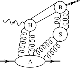
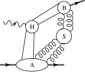
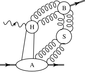
(a)	(b)	(c)
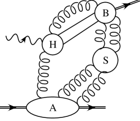
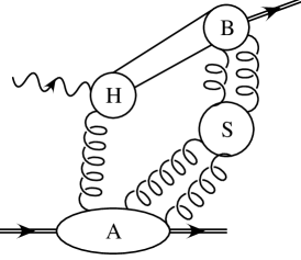
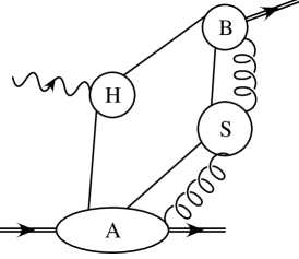
(d)	(e)	(f)

FIG. 8.: Leading regions for our process, when gluons entering the hard subgraph are transversely polarized, and when we do not explicitly indicate terms where the meson couples to a set of gluons. Each soft subgraph may have any number of external gluons, including zero.

Compared to the usual factorization theorem for inclusive scattering, the discussion is more involved, since we need to treat cases where the hard scattering amplitude has four external lines, instead of just two. So, to simplify the discussion, we will restrict our attention to the case that the collinear gluons attaching to the hard subgraph have transverse polarization. The other cases will be taken care of by gauge-invariance. The resulting list of regions is shown in Fig. 8.

First we observe that, by Eq. (28), we need to consider only hard subgraphs with at most four external quark and transverse gluon lines.

Two cases with four external lines for $H$ are (a) and (b), which have a quark-antiquark pair going from the hard scattering to the meson, and with either a gluon pair or a quark-antiquark pair joining the hard part to the proton. There is a possible soft part joined to the collinear subgraphs by arbitrarily many gluons. These terms correspond to the final factorization theorem, after a cancellation of the effects of the soft gluons. A third possibility is where all the collinear-$B$ lines of the hard subgraph are transverse gluons, as in graph (c). In this case we can make a cut of the graph such that the meson couples to gluons; such graphs we will call “glue-ball” graphs. We will find that they all cancel at the leading power $1/Q$. A fourth possibility is in graph (d), where one collinear gluon comes from the proton, and three collinear partons go to the meson. In the final factorization theorem, this would need a color octet operator in the proton factor, and such an operator has a zero matrix element between proton states.

Next we can have graphs with two or three external lines for the hard scattering, Fig. 8(e) and (f). These are harder to treat, as we will see in Sec. VII E. In fact, graph (f) will make a leading contribution in the case of a transversely polarized photon and will not make a factorization theorem of the form Eq. (7). Graph (e) will combine with those of type (a), with two collinear gluons entering the hard part, when we construct the appropriate operator product expansion.

According to Eq. (28), we have a leading $1/Q$ contribution from graph (f), where the hard part has two external quark lines, and the quark loop is completed in the soft part. But now observe that the hard part, to the leading power of $Q$, is the on-shell electromagnetic form factor of a massless quark. (Subtractions to prevent the double counting of different regions will remove the infra-red divergences of the form factor.) This form factor is proportional to

$$\epsilon_{\gamma^{*}}^{\mu}\bar{u}_{B}\gamma_{\mu}u_{A},$$ (37)

where $u_{A}$ and $u_{B}$ are Dirac wave functions for the external quarks of the hard scattering, and $\epsilon_{\gamma^{*}}$ is the polarization vector of the virtual photon. By the rules for computing a hard scattering amplitude, the momenta of the quarks are massless and are in the $+$ and $-$ directions. Since we have chosen the photon to be longitudinally polarized, $\epsilon_{\gamma^{*}}^{\mu}$ is a linear combination of the momenta of the two quarks. Hence the Dirac equation for massless spinors gives us zero for Eq. (37).

Notice that this argument does not apply when the photon is transverse; graph (f) exactly corresponds to the endpoint contribution discussed in Ref. [1]. We will discuss this issue in more detail in Sec. X.

C Other gluons joining the collinear subgraphs to the hard part

We have now seen that all the leading regions, that give the power $1/xQ$ for the amplitude have the form of Fig. 8 (a), (b) and (e), given that the photon is longitudinally polarized. For clarity, the figures are not drawn quite correctly since we have not yet treated the cancellation of gluons with scalar polarization. In the graphs, any number of extra gluons may join each collinear subgraph to the hard subgraph. An example is shown in Fig. 9. As shown in Sec. V A, the addition of extra scalar gluons does not change the power of $Q$.

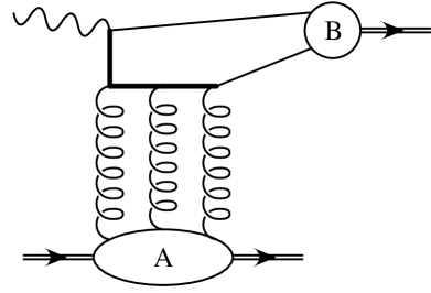
FIG. 9.: Example of region with extra gluons joining collinear subgraphs to hard subgraph. All lines are supposed to be collinear to the meson or the proton, as appropriate, except for the two thick lines, which have virtuality of order $Q^{2}$.

The fact that scalar gluons have a polarization proportional to their momentum suggests that they can be eliminated by a gauge transformation. In fact, we will use gauge invariance, in Sec. VII D, to show that only matrix elements of gauge-invariant operators are needed in the definitions of the parton-density and the wave-function factors in the factorization theorem, Eq. (7). The result will be that the contributions of scalar gluons will give the path-ordered exponentials in the gauge-invariant operators that define the distribution and density functions in Eqs. (8) and (12).

In an appropriate axial gauge, the contributions of the scalar gluons are power-suppressed, and correspondingly the path-ordered exponentials in the operators are unimportant. This fact would render the use of an axial gauge very attractive in proving factorization, were it not for the complications in treating soft gluons that result from the unphysical poles of the gluon propagator in these ‘physical gauges’. Compare the work in Refs. [8, 26] on proofs of factorization theorems for inclusive processes.

VI Subtractions

For each graph $\Gamma$, there may be several different regions of loop-momentum space that contribute to the leading power. Each region is associated with a pinch-singular surface $\pi$ of the corresponding massless graph, and we write the graph as a sum of contributions each associated with one surface:

$${\rm Asy}\,\Gamma=\sum_{\pi}\Gamma_{\pi},$$ (38)

where ‘Asy’ denotes the asymptotic behavior of the graph. In this section we will summarize the construction of the terms on the right-hand-side of this equation.

Roughly speaking, the term $\Gamma_{\pi}$ is obtained by Taylor expanding the hard and collinear subgraphs in powers of the small variables, an operation we denote by $T_{\pi}$. Since there may be more than one region contributing for a given graph, we must make subtractions which will avoid double counting; the operation of applying the subtractions we will denote by $R$, since it is a kind of renormalization. Thus we will write

$${\rm Asy}\,\Gamma=\sum_{\pi}RT_{\pi}(\Gamma).$$ (39)

This structure is completely analogous to that of the Bogoliubov $R$-operation for renormalization. The most convenient way we have found for formulating the procedure is due to Tkachov and collaborators [30]. Although the detailed exposition of the method given in [30] is tied to Euclidean problems, the general principles are not. In this method, the integrand of each graph $\Gamma$ as a distribution. Thus we define

$$\langle\Gamma,f\rangle=\int dk\,\Gamma(k,p)\,f(k),$$ (40)

where $k$ denotes the collection of loop momenta, $p$ the external momenta, and $f(k)$ is a test function. The contribution of the graph to the scattering amplitude is given by replacing the test function by unity.

The advantages of using these distributional techniques [30] stem from the fine control they give by enabling us to treat different regions of momentum space separately without having to make sharp boundaries between the different regions. This last point is particularly important in problems like ours, where it is important to be able to deform contours of integration away from non-pinch singularities; the use of sharp boundaries between regions prevents the use of contour deformation.

In this language, the contribution $\Gamma_{\pi}$ to ${\rm Asy}\,\Gamma$ from the neighborhood of a pinch-singular surface $\pi$ is localized on the surface; that is, it is proportional to a $\delta$-function (with possible derivatives) that restricts the integration to the surface. To obtain a convenient form for $\Gamma_{\pi}$, we observe that the graph is a product of a factor that is singular on $\pi$ and a factor that is non-singular there. Thus we write

$${\rm Asy}\,\Gamma(k)=\sum_{\pi}C_{\pi}(k;p,\mu)E_{\pi}(\mu),$$ (41)

where $C_{\pi}(k)$ is a distribution that is localized on the surface $\pi$ and is obtained by expanding the hard subgraph $H$ in Fig. 4 in powers of its small external variables (with appropriate subtractions). The quantity $E_{\pi}$ corresponds to the product of the singular factors, $A$, $B$, and $S$ in the reduced graph. Essentially, $C_{\pi}$ corresponds to the short distance factor on the surface $\pi$, and $E_{\pi}$ to the long-distance factor.

We will only present a summary of proof that this all works. An important observation is that the issues are identical to those for other kinds of factorization. We first define a hierarchy of regions, by simple set-theoretic inclusion: i.e., we define $\pi_{1}>\pi_{2}$ to mean that the pinch singular surface $\pi_{1}$ contains the pinch singular surface $\pi_{2}$. For any given pinch-singular surface $\pi$, we construct its corresponding term in Eq. (41) on the assumption that the terms for all bigger regions have already been constructed. Thus the construction of Eq. (41) is recursive, starting from the largest region.

Suppose, then, that we have constructed the terms $\Gamma_{\pi^{\prime}}$ for all regions bigger than $\pi$. Let us decompose ${\rm Asy}\,\Gamma$ as

$${\rm Asy}\,\Gamma=\sum_{\pi^{\prime}>\pi}\Gamma_{\pi^{\prime}}+\Gamma_{\pi}+\mbox{other terms}.$$ (42)

The “other terms” correspond to the three classes of surface that are illustrated in Fig. 10:

• Those that are smaller than $\pi$.

• Those that intersect $\pi$ in a subset (necessarily a manifold of lower dimension).

• Those that do not intersect $\pi$ at all.

We assume as an inductive hypothesis that the sum of $\Gamma_{\pi^{\prime}}$ over $\pi^{\prime}>\pi$ gives a good approximation to the original $\Gamma$ except in neighborhoods of the smaller surfaces for which $\Gamma_{\pi}$ has not yet been constructed. The integrals defining the $\Gamma_{\pi^{\prime}}$’s cover the whole of the space of integration variables, but they are only required to give good approximations when one excludes neighborhoods of smaller surfaces; more precisely we will require them only to give good approximations when the test function in Eq. (40) has a zero of an appropriate strength on these smaller surfaces.

FIG. 10.: Illustrating the three classes for the “other terms” in Eq. (42).

We now construct $\Gamma_{\pi}$. When combined with the $\Gamma_{\pi^{\prime}}$ for larger surfaces it must give a good approximation to $\Gamma$ on a neighborhood of $\pi$. It is sufficient for our purposes to require only that we have a good approximation when the test function has an appropriate zero on the smaller surfaces. It is not necessary to have constructed $\Gamma_{\pi^{\prime}}$ for the smaller surfaces, since they will give zero with such a test function. This is sufficient to prove the inductive hypothesis for the next use of the recursion.

Since $\Gamma_{\pi}$ is localized on the surface $\pi$, it is necessary only to consider a neighborhood of $\pi$. This combined with our remarks in the previous paragraph ensures that we do not need the unconstructed “other terms” in Eq. (42) in order to construct $\Gamma_{\pi}$.

Therefore we define

$$\Gamma_{\pi}=T_{\pi}\left(\Gamma-\sum_{\pi^{\prime}>\pi}R\Gamma_{\pi^{\prime}}\right),$$ (43)

where $T_{\pi}$ represents the Taylor expansion in powers of the small variables on $\pi$. The first term is the Taylor expansion of the original graph, and the remaining terms can be thought of as subtractions that prevent double counting of contributions to the integral over a neighborhood of $\pi$.

The result is that a sum over $\Gamma_{\pi}$ and the terms for larger regions,

$$\Gamma_{\pi}+\sum_{\pi^{\prime}>\pi}R\Gamma_{\pi^{\prime}},$$ (44)

correctly gives the contribution to the asymptotics of $\Gamma$ that comes from a neighborhood of $\pi$ and of all larger regions, but with neighborhoods of smaller regions being excluded.

Now, in general, $\Gamma_{\pi}$ gives a divergence when we integrate it with a test function over a neighborhood of any of these smaller regions. So it is defined only when integrated with a test function that is zero on these smaller regions. We now extend it to a distribution defined on all test functions by adding infra-red counterterms to cancel the divergences. (We will not specify the details, but just observe that the construction is exactly analogous to the construction of the well-known distribution $(1/x)_{+}$.) We call the result $R\Gamma_{\pi}$. The counterterms are local in momentum space. Since we have not yet considered how to approximate $\Gamma$ in regions smaller than $\pi$, it is perfectly satisfactory that we can choose a definition of $\Gamma_{\pi}$ on the smaller surfaces. We only require that the result, $R\Gamma_{\pi}$, be finite, and that the counterterms be localized on smaller surfaces than $\pi$, so that we do not affect the good approximation we have already obtained for $\pi$ and larger surfaces.

In the later stages of the recursion, we obtain the appropriate approximations for these smaller regions. The subtraction terms, as defined in Eq. (43), ensure that changes in the choice of counterterms localized on any particular surface $\pi$ are cancelled by corresponding changes in the subtraction terms when we define $\Gamma_{\pi}$. Hence the overall result for the asymptotic expansion of $\Gamma$ is independent of these choices.

This completes the summary of the construction of the ${\rm Asy}\,\Gamma$.

VII Completion of proof

A Summary of previous results

The results so far can be summarized in Eq. (39). In the asymptotic large $Q$ limit, each graph is written as a sum of contributions from a set of regions. We have identified the regions and computed the power of $Q$ associated with each region.

Any particular region can be conveniently summarized by a diagram of the form of Fig. 4. It is specified by a decomposition of a graph $\Gamma$ into two collinear subgraphs, $A$ and $B$, a soft subgraph, $S$, and a hard subgraph, $H$. When we sum Eq. (39) over all graphs $\Gamma$, we can represent the result by independent summations over the possibilities for the subgraphs $A$, $B$, $S$, and $H$:

$${\rm Asy}\,{\cal M}=\sum_{\Gamma}{\rm Asy}\,\Gamma=A\times B\times S\times H.$$ (45)

Here, $A$, for example, represents the sum over all possibilities for a collinear-to-$A$ subgraph. Implicit in Eq. (45) are appropriate Taylor expansions in small variables, together with suitable subtractions to avoid double counting, etc. The symbol $\times$ represents integrations over the momenta of loops that circulate between the different factors and also a summation over the flavors of the parton lines joining the different subgraphs.

Each subgraph comes with a specification of its external lines, and the summation is restricted to compatible subgraphs. For example, in Fig. 8(a) we require that $H$ have as its external lines two collinear-to-$A$ gluons, a collinear-to-$B$ quark, a collinear-to-$B$ antiquark, and the virtual photon. To be compatible with this, the subgraph $A$ must have as its external lines two collinear gluons, as well as the hadrons $p$, $p^{\prime}$ and the soft gluons. Such restrictions can be enforced by a suitable definition of the $\times$ operation in Eq. (45).

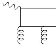
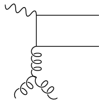
(a)	(b)

FIG. 11.: (a) An allowed graph, and (b) a disallowed graph for a hard part whose external lines are two collinear-to-$A$ gluons, a collinear-to-$B$ quark, a collinear-to-$B$ antiquark, and a photon.

As always for a hard subgraph, it is required that $H$ be one-particle-irreducible (1PI) in the $A$ lines and the $B$ lines. Thus, Fig. 11(a) is allowed as a hard subgraph. However, Fig. 11(b) is not allowed, since it has an internal line (the vertical gluon) that is forced to be collinear (by the two external gluons).

B Taylor expansion: collinear case

We now Taylor expand the factors in Eq. (45) in powers of small variables. To understand the general principles by which this operation gives the factorization theorem, with its operator definitions of the collinear factors, let us first treat the case that there is no soft factor and that exactly two lines connect each collinear graph to the hard part—Fig. 12. We then have

$$A\times B\times H = \int d^{4}k_{A}\,d^{4}k_{B}\,A(k_{A},\Delta-k_{A})\,B(k_{B},V-k_{B})\,H(q,k_{A},\Delta-k_{A},k_{B},V-k_{B})$$ (46)

$$\simeq \int d^{4}k_{A}\,d^{4}k_{B}\,A(k_{A},\Delta-k_{A})\,B(k_{B},V-k_{B})$$ (48)

$$~{}H\!\left(q,(k_{A}^{+},0,0_{\perp}),(\Delta^{+}-k_{A}^{+},0,0_{\perp}),(0,k_{B}^{-},0_{\perp}),(0,V^{-}-k_{B}^{-},0_{\perp})\right).$$

The notation is unfortunately cumbersome, but it makes precise the operations we have applied to the hard part: We have replaced the momenta collinear to $A$ by their $+$ components, and the momenta collinear to $B$ by their $-$ components. This represents the first term in the expansion of $H$ in powers of the other components of these momenta.

FIG. 12.: Simple region: collinear and hard subgraphs only, with two lines joining each collinear graph to the hard subgraph.

Only the $k_{A}^{+}$ and $k_{B}^{-}$ integrals now couple the different factors. This gives

$$A\times B\times H \simeq \int dk_{A}^{+}\,dk_{B}^{-}\,\,$$ (51)

$$\int dk_{A}^{-}\,d^{2}k_{A\perp}\,A(k_{A},\Delta-k_{A})\,\,\int dk_{B}^{+}\,d^{2}k_{B\perp}\,B(k_{B},V-k_{B})$$

$$~{}H\!\left(q,(k_{A}^{+},0,0_{\perp}),(\Delta^{+}-k_{A}^{+},0,0_{\perp}),(0,k_{B}^{-},0_{\perp}),(0,V^{-}-k_{B}^{-},0_{\perp})\right),$$

which has the general structure of the factorization formula Eq. (7). To see this more explicitly, we observe that:

• Scaling $k_{A}^{+}$ and $k_{B}^{-}$ by factors of $p^{+}$ and $V^{-}$, respectively, gives the integration variables $x_{1}$ and $z$ in Eq. (7).

• The factor $A$ is a matrix element of a time-ordered product of two fields. Integrating over all $k_{A}^{-}$ and $k_{A\perp}$ puts the difference of coordinates of the two fields on the light-like line $(0,y^{-},0_{\perp})$. This is a matrix element of an operator like those in the definition of the parton density Eq. (8).

• Similarly, the $B$ factor becomes like the meson wave function Eq. (12).

At this point we have matrix elements of light-cone operators that consist of two operators that are integrated along a light-like line.

C Taylor expansion with soft factor; Glauber region

To complete the proof, we now have to deal with the soft factor in an analogous fashion and to show that the only operators we need are the precise ones in the definitions Eq. (8)–(12). It is convenient to start by considering $A\times S$ and $H\times B$ as units. Then we write

$$A\times B\times S\times H = \left(\prod_{i}d^{4}k_{i}\right)\,H\times B(q,V,k)\,\,A\times S(p,p^{\prime},k)$$ (52)

$$= \left(\prod_{i}d^{4}k_{i}\right)\,{\cal H}(q,V,k)\,\,{\cal A}(p,p^{\prime},k),$$ (53)

where, the $k_{i}$’s are the loop momenta coupling the two factors. Notice that ${\cal H}\equiv H\times B$ is 1PI in the lines entering it from ${\cal A}\equiv A\times S$, because any linear combination of momenta that are each collinear to $A$ or soft is itself collinear to $A$ or soft. On the other hand, ${\cal A}=A\times S$ includes all graphs with the appropriate number of external lines.

Clearly we may neglect the components $k_{i}^{-}$ of the soft momenta within ${\cal H}=H\times B$, since by definition the momenta in both $B$ and $H$ have $-$ components of order $Q$. We may also neglect $k_{i\perp}$ within $H$. But to derive the factorization theorem, we will also need to neglect $k_{i\perp}$ within the $B$ subgraph. In a general situation this is not necessarily true, since the broadest definitions of soft momenta and collinear-to-$B$ momenta only insist that their $\perp$ components be small without specifying their relative sizes. Hence one cannot always neglect a soft transverse momentum with respect to a collinear transverse momentum.

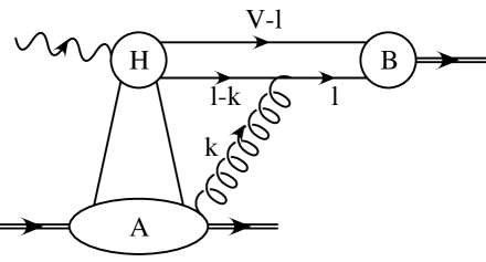
FIG. 13.: When $k$ is soft, this graph illustrates the need for contour deformation of $k^{+}$.

We use a version of the argument devised by Collins and Sterman [26] for proving factorization for inclusive processes in $e^{+}e^{-}$ annihilation. The graph of Fig. 13 illustrates the problem and its solution. We choose the gluon momentum $k$ to be soft, and the quark momentum $l$ to be collinear to the meson. The momenta in the $A$, $B$, and $H$ subgraphs are, of course, chosen to be collinear-to-$A$, collinear-to-$B$, and hard, respectively. Consider the integral over $k^{+}$, whose size is much less than $Q$, since $k$ is soft. For this reason, we neglect $k^{+}$ in the subgraphs $A$ and $H$, and the only $k^{+}$ dependence is from the $S$ and $B$ subgraphs

$$\int_{{\rm soft~{}}k}dk^{+}\,\frac{1}{[(l-k)^{2}-m^{2}+i\epsilon]\,(k^{2}+i\epsilon)}$$ (54)

$$= \int_{{\rm soft~{}}k}dk^{+}\,\frac{1}{[2(l^{+}-k^{+})(l^{-}-k^{-})-(l_{\perp}-k_{\perp})^{2}-m^{2}+i\epsilon]\,(2k^{+}k^{-}-k_{\perp}^{2}+i\epsilon)}$$ (55)

$$\simeq \int dk^{+}\,\frac{1}{[2(l^{+}-k^{+})l^{-}-(l_{\perp}-k_{\perp})^{2}-m^{2}+i\epsilon]\,(2k^{+}k^{-}-k_{\perp}^{2}+i\epsilon)},$$ (56)

where we have omitted inessential numerator factors. In the second line of this equation, we have neglected $k^{-}$ with respect to the large variable $l^{-}$. Except for $l^{-}$, all the momentum components used in this equation are small compared with $Q$.

We distinguish two cases:

1. $k^{+}k^{-}\gtrsim k_{\perp}^{2}$. In this case, we can indeed neglect $k_{\perp}$ in the first denominator. Because $k$ is soft, while $l$ is collinear to $B$, the terms involving $k_{\perp}$ are small compared with the $k^{+}l^{-}$ term.

2. $k^{+}k^{-}\ll k_{\perp}^{2}$. This is called the Glauber region in the terminology of [32]. In this region $k^{+}l^{-}$ may be comparable to $k_{\perp}^{2}$, so that we apparently cannot neglect $k_{\perp}$ in the collinear subgraph $B$. However, in this region the only dependence on $k^{+}$ is in the collinear propagator, and so we may deform the $k^{+}$ contour into the complex plane until we recover the first case.

So in fact we can neglect $k_{\perp}$ as well as $k^{-}$ in the collinear propagator.

In general, we will have several soft momenta $k_{i}$ entering the $B$ subgraph, and to use the above proof, we must ensure that none of the collinear propagators give obstructions to the contour deformations for each $k_{i}^{+}$. In other words, all the poles must be on one side of the real axis for each $k_{i}^{+}$. To prove this [26], we note that all the collinear-to-$B$ lines go forward from the hard scattering, but not backward—compare the reduced graphs in Fig. 7. Thus we can route all the $k_{i}^{+}$’s back along collinear lines to the hard scattering, and thus all the poles that collinear propagators give are in the upper-half-plane, just as in Eq. (56).

It should be observed that we cannot apply the same argument to the $k^{-}$ dependence of the $A$ subgraph, since we have collinear-to-$A$ lines both before and after the hard scattering. This fact alone resulted in enormous complications in the proof of factorization in the Drell-Yan process [8, 9].

D Gauge-invariance

Now that we have proved that the $+$ and $\perp$ components of soft momenta may be neglected in both $B$ and $H$, we can write

$$A\times B\times S\times H\simeq\int\prod_{i}dk_{i}^{+}\,{\cal H}(q,V,k^{+})\left(\int\prod_{i}dk_{i}^{-}d^{2}k_{i\perp}\,\,{\cal A}(p,p^{\prime},k).\right)$$ (57)

This gets us much closer to the desired factorization. It is exactly a kind of operator product expansion, since the ${\cal A}$ factor is a matrix element of a light-cone operator, apart from the consequences of subtractions. In fact, the subtractions needed to define ${\cal A}$ are associated with regions with larger singular surfaces, and thus in fact to ultra-violet divergences associated with the operator vertices. That is, the subtractions are just an implementation of the ultra-violet counterterms needed to define renormalized operators. We therefore write Eq. (57) as

$$A\times B\times S\times H\simeq\sum_{i}C_{i}(q,V,k^{+})\,O_{i}(p,p^{\prime},k^{+}),$$ (58)

where the $O_{i}$ are the matrix elements of renormalized light-cone operators, and we will call the $C_{i}$’s coefficient functions. We use $i$ to label the different possible operators.

But there are many possible operators, even when we restrict ourselves to the leading power. Each case of the graphs of Fig. 8 with a different set of external lines for the $A\times S$ graph corresponds to a different operator. But now we can appeal to the new results by Collins [33]. These show that we can restrict the sum to gauge invariant operators. Such operators consist of gauge covariant operators (like $G_{\mu\nu}$, $\psi$) joined by path-ordered exponentials (often called “string operators”).

We must now determine which of these operators is needed to give a leading power. First, we construct a modified version of the decomposition of gluons into scalar and transverse polarizations. Consider one particular external gluon, of momentum $k$, that attaches ${\cal A}$ to ${\cal H}$. We have a factor

$${\cal A}^{\mu}(k)\,g_{\mu\nu}\,{\cal H}^{\nu}(k^{+}),$$ (59)

where $g_{\mu\nu}$ is the numerator of the gluon propagator. Recall, from Sec. V, that the largest term in the sum over the vector indices is the one with $\mu=+$ and $\nu=-$, i.e., ${\cal A}^{+}{\cal H}^{-}$. This happens because the collinear subgraphs are highly boosted in the Breit frame and after the boosts the ${\cal A}^{+}{\cal H}^{-}$ term is the one with the largest components. The arguments apply both to the connection of collinear-to-$A$ lines to the hard subgraph $H$ and of soft lines to the collinear-to-$B$ subgraph $B$, i.e., to all the gluons connecting ${\cal A}$ to ${\cal H}$.

From the point of view of the ${\cal H}$ factor, the gluon $k$ is an on-shell massless gluon with a polarization vector proportional to ${\cal A}^{\mu}$, and a momentum in the $+$ direction: $k^{\prime}\equiv(k^{+},0,0_{\perp})$. The big term in ${\cal A}\cdot{\cal H}$ therefore corresponds to a polarization exactly proportional to the momentum of the gluon. This we call a scalar gluon, and we therefore make the following decomposition:

$${\cal A}^{\mu}=p_{A}^{\mu}\frac{{\cal A}\cdot p_{B}}{p_{A}\cdot p_{B}}\,+\,\left({\cal A}^{\mu}-p_{A}^{\mu}\frac{{\cal A}\cdot p_{B}}{p_{A}\cdot p_{B}}\right).$$ (60)

To make a covariant formula, we used the previous definitions that $p_{A}$ and $p_{B}$ are vectors purely in the $+$ and $-$ directions. The first term on the right-hand-side of this equation we label as corresponding to scalar polarization, and the second term as corresponding to transverse polarization. Since the scalar polarization is exactly proportional to the approximated momentum $k^{\prime}$ used in ${\cal H}$, it gives a factor $k^{\prime}\cdot{\cal H}(k^{\prime})$. This is precisely the kind of situation in which Ward identities simplify the sum over all graphs. The indirect methods of Ref. [33] give a very efficient implementation of the relevant identities.

With the modified definitions, it is still true that there is no penalty for attaching a scalar gluon to ${\cal H}$, but that there is a penalty for every transverse gluon line and every quark line. Now, the factors for the external lines of ${\cal A}$ correspond to the Feynman rules for light-cone operators. So scalar gluons are associated with factors of $A^{+}$ in an operator, where $A^{+}$ is the $+$ component of the gluon field. The gauge invariant gluon operator with the lowest number of transverse gluons is of the form

$$G^{i+}(0,y^{-},0_{\perp})\,{\cal P}\,G^{j+},$$ (61)

where ${\cal P}$ is a path-ordered exponential of the gluon field. The indices $i$ and $j$ label transverse components. Notice that the operator associated with the scalar gluons, $A^{+}$, is exactly the one that appears, exponentiated, in ${\cal P}$.

The operator, Eq. (61), is a $2\times 2$ matrix on transverse coordinates. We now find the restrictions due to angular momentum conservation that restrict those components of this matrix that have a non-zero coupling to the hard scattering. Consider the hard part times the meson wave function as a scattering process for collinear gluons plus the virtual photon to make the meson. Angular momentum conservation plus the fact that the photon is longitudinally polarized implies that the angular momentum of the gluons around the collision axis equals the helicity of the meson.

The matrix has components of helicities 0, $+2$ and $-2$. So if the meson is a transversely polarized vector, then we have a zero hard part, as indicated on the fourth line of Eq. (14).

If the meson is a longitudinally vector or a pseudo-scalar meson, then either of the two matrices of zero helicity contribute:

$$\left(\begin{array}[]{cc}1&0\\ 0&1\end{array}\right),\ \ \left(\begin{array}[]{cc}0&i\\ -i&0\end{array}\right).$$ (62)

Parity conservation implies that the first matrix is the only one to which the hard scattering couples for the case of a longitudinal vector meson. For the factorization theorem for longitudinal vector mesons, we therefore find that the gluon density needed is the one defined in Eq. (10); it defines the ${\cal A}$ factor, with the normalization factor being a matter of convention.

For case of pseudo-scalar mesons, the second matrix in Eq. (62) is the one that satisfies parity invariance. However, charge-conjugation invariance, as indicated below Eq. (13), implies that the hard-scattering coefficient is zero.

Similar arguments give Eq. (8) as the definition containing the smallest relevant gauge-invariant operator with quarks, when we are treating production of longitudinally polarized vector mesons, with Eq. (12) being the definition of the meson wave function. The $\gamma^{+}$ factor in Eq. (8) picks out the largest components of the quark and antiquark fields.

Next we apply the same arguments about angular momentum conservation to the production of pseudo-scalar mesons and of transversely polarized vector mesons. We find that the changes needed in the definitions of the parton densities and the wave functions are those indicated in Eqs. (13) and (14).

In our expansion of the form of Eq. (58), the operators can be expanded in powers of the fields in the path-ordered exponentials. Thus we may regard Eq. (58) in two equivalent ways. One way is to restrict the operators to exactly the gauge invariant operators. The number of terms is then $2N_{f}+1$: one operator for each flavor of quark and antiquark and one for the gluon. Another way to look at the formula is to sum over terms for each of the operators obtained in the expansion of the gauge-invariant operators. This gives an infinity of terms, but in $2N_{f}+1$ groups, with identical Wilson coefficients within each group.

The second point of view is useful because it shows that, to obtain the coefficient $C_{i}$ for each gauge-invariant operator, it is sufficient to examine graphs for the $H\times B$ factor that have the minimum number of external lines, viz., two transverse gluons or two quarks (in addition to the photon and the meson).

E Endpoint contributions

We have now shown that the leading power for our amplitude is given by a convolution of operator matrix elements for the proton, times coefficients that are obtained from hard subgraphs times collinear subgraphs associated with the meson. The coefficients are obtained from graphs for ${\cal H}=H\times B$ with exactly the two external lines that correspond to the two parton fields in Eqs. (8) and (10) that we have when the path-ordered exponentials are omitted in the operators.

Only if both external lines connect to the hard part can we proceed to the next step of factoring $H\times B$ into the hard factor in the factorization formula times the wave-function factor Eq. (12). Unfortunately, the external lines of $H\times B$ can connect either to the hard subgraph or to the collinear subgraph, a situation summarized in the following equation:

$$\raisebox{-18.06749pt}{\epsfbox{hb.eps}}~{}=\raisebox{-18.06749pt}{\epsfbox{h2b0.eps}}~{}+\raisebox{-18.06749pt}{\epsfbox{h1b1.eps}}.$$ (63)

The first term corresponds to the region of Fig. 8(b), and the second to Fig. 8(f), in the case that there are no extra gluons attaching $S$ to $B$. The dots between the $H$ and $B$ subgraphs indicate an arbitrary number of lines being exchanged.

A similar equation applies with external gluons, and corresponds to the regions of Fig. 8(a), (d), and (e). Note that the gluon attaching to $B$ now has to be transverse, so that we have lost one power of $Q$ for graph (e), which has only three partons connecting to the hard subgraph. This brings the power for all cases down to $1/Q$, and hence there are no further power law cancellations that we will need to take into account.

In Eq. (63), we call the term where one of the lines attaches to $B$ an “end-point” contribution, for the following reason. In the factorization equation (7), the longitudinal momentum fractions of the two lines relative to the incoming proton are $x_{1}$ and $x-x_{1}$. When one of the lines attaches to $B$, that means that the line is soft, that is, that we are examining the contribution of a small neighborhood of either $x_{1}=0$ or $x-x_{1}=0$. We can equally well think of the contribution as being obtained from a region of the form of Fig. 8(a) or (b), when one of the quarks joining the meson to the hard part becomes soft. That is, the term can also be thought of as related to one of the endpoints $z=0$ or $z=1$ of the $z$ integral.

Suppression of endpoint contribution for longitudinal photon: According to our power counting formula, the end-point contribution is leading, being proportional to $1/Q$. There is in fact an additional suppression. Consider Fig. 8(e). The hard part is proportional to

$$\epsilon_{g}^{i}\epsilon_{\gamma}^{\mu}h_{i\mu},$$ (64)

where $\epsilon_{g}$ and $\epsilon_{\gamma}$ are the polarizations of the gluon and photon, and the gluon index $i$ is purely transverse. The tensor $h_{i\mu}$ is obtained from the diagrams with a trace with $\gamma^{+}$. Thus $h_{i\mu}$ is a tensor constructed from vectors in the $+$ and $-$ direction and from the metric tensor. It is therefore zero when $g=+$ or $\mu=-$, and therefore we get a zero when the photon is longitudinally polarized. The proofs we have made previously are appropriate for the leading power of $Q$, so the zero corresponds to a suppression by another power of $Q$. Recall that we have already proved that at least one of the gluons joining $S$ to $B$ must be transverse, and that results in a suppression compared with the $Q^{0}$ given by the power-counting formula.

We therefore conclude that the endpoint contribution from Fig. 8(e) is of order $1/Q^{2}$. Since we have already proved—around Eq. (37)—the corresponding result for Fig. 8(f), where the hard scattering has two quark lines, we now know that all endpoint contributions are suppressed, and we saw above that this is sufficient to obtain the factorization theorem.

But clearly, the situation is different when the photon is transversely polarized. We will discuss this further in Sec. X.

F End of proof

We have now proved that the endpoint contributions are power-suppressed, in the case that the photon has longitudinal polarization. So the only term that survives in Eq. (63) is the one where both partons from the proton attach to the hard scattering.

We can now apply the operator expansion argument to the $H\times B$ factor, to obtain the product of a coefficient times a suitable vacuum-to-meson matrix element. The matrix element is the one given in Eq. (12), with no purely gluonic operator being allowed, because of our choice for the quantum numbers of the meson. This result immediately gives the factorization theorem, Eq. (7), provided only that we adjust the normalization of the hard-scattering factor appropriately.

VIII Evolution equations

The definitions of the off-diagonal parton densities, Eq. (8) and (10), are just the same as those of the ordinary diagonal parton densities. In both cases, there are ultra-violet divergences and corresponding anomalous dimensions. The divergences are properties of the operators themselves. Since the same operators appear in the light-cone wave function, Eq. (12), this permits us to give a unified treatment for both the parton densities and the wave functions.

The resulting renormalization-group equations give the DGLAP evolution that is essential to phenomenology. The two non-perturbative factors in the factorization theorem depend on a renormalization/factorization scale $\mu$. We need to choose it of order $Q$ in order to make effective perturbative calculations of the hard scattering factor. Therefore we need the evolution equations with respect to $\mu$, in order to compute predictions in terms of the non-perturbative factors evaluated at a fixed scale.

Only minor generalizations in previously existing treatments for the diagonal densities are needed [17]. Balitsky and Braun [34] have given a more general treatment, and recently Ji and Radyushkin [12, 13, 14] treated exactly the operators we are considering.

The essential point is that the ultra-violet divergences arise when momenta get infinite in a subgraph attached to the operator vertex. The relevant regions of loop momentum can be labeled by diagrams of the form of Fig. 14, which is to be interpreted in a similar fashion to those for the leading regions for the scattering amplitude itself.

FIG. 14.: Regions for UV divergences of parton densities. The momenta in the upper blob have large virtualities, and the momenta in the lower blob are collinear to the hadron. Removing one external hadron gives the regions for UV divergences of light-cone wave functions.

After use of gauge invariance to make a kind of operator product expansion, the divergences will be of the form of the parton densities themselves convoluted with ultra-violet renormalization factors. Hence the right-hand side of the evolution equation is of the form of a kernel convoluted with the parton densities. The derivation and the result is just the same as for the diagonal densities, except that one must take account of the longitudinal momentum flow in the $t$-channel. For the distributions, we have

$$\mu\frac{d}{d\mu}f_{i/p}(x_{1},x_{2},t,\mu)=\sum_{j}\int d\xi P_{ij}(x_{1},x_{2},\xi;\alpha_{s}(\mu))f_{j/p}(\xi,x_{2}-x_{1}+\xi,t,\mu).$$ (65)

When $t=0$ and $x_{1}=x_{2}=x$, the equation reduces to the standard Altarelli-Parisi equation, with a kernel $\xi P_{ij}(x,x,\xi;\alpha_{s}(\mu))$. Since the ultra-violet divergences are independent of the transverse and $-$ components of momenta, the kernel $P_{ij}$ is independent of $t$.

This implies that when the individual momentum fractions $x_{1}$ and $x_{2}$ are much larger than $x\equiv x_{1}-x_{2}$, the distributions approach the diagonal ones, and the limit $x_{1}=x_{2}$ can be taken in the kernel.

The same operator occurs in the meson’s light-cone wave function, so that its evolution equation contains the same kernel

$$\mu\frac{d}{d\mu}\phi^{V}_{i}(z,\mu)=\sum_{j}\int d\zeta P_{ij}(z,\zeta;\alpha_{s}(\mu))\phi^{V}_{j}(\zeta,\mu).$$ (66)

Corresponding Altarelli-Parisi equations apply to the other parton densities and wave functions needed for treating the production of pseudo-scalar mesons and transversely polarized vector mesons.

IX Rules for Hard scattering function

The hard scattering function $H_{ij}$ in Eq. (7) is obtained from graphs with the appropriate external parton lines for the $H$ subgraph Fig. 8(a) and (b). The graphs are 1PI in the two lines from the proton and in the two lines from the meson. Lowest order graphs are given in Fig. 2. Subtractions are made to cancel the collinear divergences. Minimal subtraction can be used for the subtractions just as in inclusive hard scattering, and in the same fashion. Normal Feynman rules are applied to the interior of the graphs, so it remains to construct the normalization factors and the external line factors.

Consider first graphs in which the proton factor is connected by quark lines to the hard scattering. The leading power is obtained from a factor of the form

$${\rm tr}\,\left(\mbox{$\gamma^{+}$ part of $H$}\times\mbox{$\gamma^{-}$ part of $A$}\right),$$ (67)

which we can write as

$$\frac{1}{2}{\rm tr}\,(\gamma^{-}H)\,\frac{1}{2}{\rm tr}\,(\gamma^{+}A).$$ (68)

The $1/2$ and the $\gamma^{+}$ in the second factor appear directly in the definition of the parton density, Eq. (8), with the $1/2$ multiplying a $1/2\pi$ associated with the Fourier transform.

As to the integral over the loop momentum $k$ connecting $A$ and $H$, the $1/(2\pi)^{4}$ factor is completely inside the parton density, as are the integrals over the transverse and $-$ components of the momentum. We rewrite the integral over $k^{+}$ as

$$\int dk^{+}\,\dots=\int dx_{1}\,p^{+}\dots.$$ (69)

In addition there is a trace over color indices between $A$ and $H$. Since $A$ is a unit matrix in color space—the protons are color singlet—and since the parton density is defined to include a sum over colors, we need to trace $H$ over color and divide by the number of quark colors, $N_{c}=3$.

Hence the external line factor associated with quarks entering the hard scattering from the proton blob is

$$\mbox{$A$-quark factor}=\frac{1}{2N_{c}}p^{+}\,\,{\rm tr}\,\gamma^{-}\dots,$$ (70)

with the trace being over both Dirac and color indices, and where “$\dots$” represent the rest of the hard subgraph, with ordinary Feynman rules. The factor $1/2N_{c}$ is in effect an average over spin and color, just as we would have in an inclusive process.

With one exception, exactly similar considerations apply to the connection of the hard scattering to the meson factor, apart from a need to exchange the $+$ and $-$ coordinates. The exception is that the definition Eq. (12) of the wave function contains an extra factor $1/\sqrt{2N_{c}}$. Hence the external line factor associated with quarks entering the hard scattering from the meson blob is

$$\mbox{$V$-quark factor}=\frac{1}{\sqrt{2N_{c}}}V^{-}\,\,{\rm tr}\,\gamma^{+}\dots.$$ (71)

Finally there is the case of gluons attaching the proton blob to the hard subgraph. Here we get similarly

$$\mbox{$A$-gluon factor}=\frac{1}{2(N_{c}^{2}-1)}\delta_{ij},$$ (72)

where we have an average over the two transverse polarizations and the $N_{c}^{2}-1$ colors of a gluon.

X Transversely polarized photons

Our proof of the factorization theorem Eq. (7) is valid when the photon is longitudinally polarized, since we were able to show that the contribution of endpoint regions was power suppressed. Order-by-order in perturbation, an amplitude of order $1/Q$ times logarithms was obtained, but with an enhancement due to scaling violations when we apply DGLAP evolution.

In this section we will show that the amplitude for transversely polarized photons is suppressed by one power of $Q$. First we will show this for the non-endpoint contribution, as a consequence of Lorentz invariance. Then we will treat the endpoint terms.

A Power-counting: non-endpoint case

Consider first the non-endpoint contributions, where the hard scattering has four external lines, Fig. 8(a) and (b). For region (a), the hard part has a polarization-dependence of the form

$$\epsilon_{1}^{i}\epsilon_{2}^{j}\epsilon_{\gamma^{*}}^{\mu}h_{ij\mu},$$ (73)

where $\epsilon_{1}$ and $\epsilon_{2}$ are the transverse gluon polarizations, and $h_{ij\mu}$ is a tensor constructed out of longitudinal vectors and out of Lorentz invariants. The tensor is therefore invariant under rotations in the transverse plane, and hence it can only be nonzero if $\mu=+$ or $\mu=-$. So we get a non-zero result for the leading power only for a longitudinally polarized photon.

For the quark graph, 8(b), the result is even simpler, since after the trace over Dirac matrices, the hard part just gives a vector

$$\epsilon_{\gamma^{*}}^{\mu}h_{\mu}.$$ (74)

The same argument that we applied to Eq. (73) gives exactly the same result.

Therefore in the case of the non-endpoint contribution the leading $1/Q$ power is only obtained when the photon is longitudinally polarized. There must be at least a $1/Q$ suppression for transversely polarized photons, which gives a final power $1/Q^{2}$. Now in Sec. VII E, we showed that the endpoint terms obey exactly the opposite rule: longitudinal photons are suppressed, and transverse photons give the $1/Q$ contributions.

B How soft is soft?

However, to get the $1/Q$ contribution with a transverse photon, we depend on the soft momenta being treated as having a magnitude of $m^{2}/Q$. This is evidently very small: the corresponding virtuality is of order $m^{4}/Q^{2}$. Clearly, we must expect non-perturbative confinement effects to restrict all significant virtualities to being $m^{2}$ or larger. We now show that this results in a power suppression.

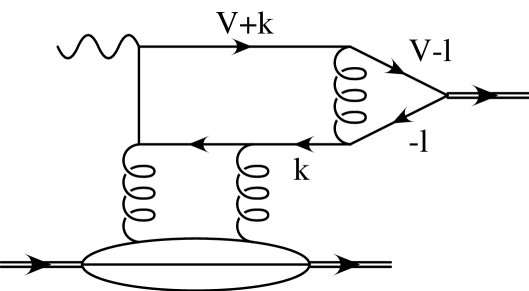
FIG. 15.: Graph to illustrate endpoint contribution with transversely polarized photon.

To see what is happening, let us examine a particular graph, Fig. 15. There are many ways in which regions of the form of Fig. 4 can be constructed. For our purposes it will be sufficient to restrict our attention to cases where the momentum $l$ that goes through the meson vertex is always collinear to $B$ and not close to either of its endpoints. Similarly, we choose all momenta in subgraph $A$ to be collinear to $A$.

The region of interest for this purpose is where the loop momentum $k$ becomes soft. So let us suppose that all components of $k$ are of order $\lambda Q$, where $\lambda$ is a parameter that we will vary between $m^{2}/Q^{2}$ and unity. The upper limit of this range is where $k$ becomes a hard momentum, and the lower limit is where $k^{\pm}$ become comparable to the small components of collinear momenta. Thus when $\lambda$ is outside of these limits we get a power-law suppression.

All the propagators and loop integrals give factors of order unity except for those in the loop $k$. So we just need to focus our attention on the following factor:

$$\int d^{4}k~{}{\rm tr}\, \left[\not\!\epsilon_{\gamma^{*}}\frac{\not\!V+\not\!k}{(V+k)^{2}}\frac{1}{(k+l)^{2}}\gamma^{\mu}\not\!B\gamma_{\mu}\frac{\not\!k}{k^{2}}\not\!\epsilon_{1}\frac{\not\!A_{1}+\not\!k}{(A_{1}+k)^{2}}\not\!\epsilon_{2}\frac{\not\!A_{2}+\not\!k}{(A_{2}+k)^{2}}\right].$$ (75)

Here $A_{1}$ and $A_{2}$ represent two collinear momenta associated with the two lower gluons, while $\epsilon_{1}$, $\epsilon_{2}$ and $\epsilon_{\gamma^{*}}$ are the polarizations of these two gluons and of the photon. We use $B^{\mu}$ to denote a collinear vector associated with the right-hand-loop through the meson. In $(+,-,\perp)$ coordinates, the magnitudes of the $A$ and $B$ momenta are

$$A_{1}^{\mu},A_{2}^{\mu} \sim \left(Q,\frac{m^{2}}{Q},m\right),$$ (76)

$$B^{\mu} \sim \left(\frac{m^{2}}{Q},Q,m\right).$$ (77)

Hard region for $k$: When $\lambda\sim 1$, so that all components of $k$ are of order $Q$, we get an overall power $1/Q$ made up as follows:

• $Q^{4}$ for the integration $d^{4}k$.

• $1/Q^{10}$ for five hard denominators.

• $Q^{5}$ for the five numerators, each of which has at least one term of order $Q$.

As always, we are working in the Breit frame. The power $1/Q$ is exactly what we obtained from general arguments; the hard subgraph consists of the $k$ loop and has external line four partons and the photon. Given the cancellations proved in Sec. VII D, we know that we can take the gluon polarizations to be transverse; this fact was used in obtaining the power of $Q$ for the numerator. Furthermore, the argument in Sec. X A shows that after the integration over the azimuth of $k_{\perp}$, the power $1/Q$ is only obtained when the photon has longitudinal polarization; one power of $Q$ is lost for transverse polarization.

Soft region for $k$: Next we consider smaller values of $\lambda$. There are two ranges to consider: $1>\lambda>m/Q$ and $m/Q>\lambda>m^{2}/Q^{2}$. The breakpoint $\lambda=m/Q$ between the two ranges occurs where the components of $k$ are comparable to masses and typical collinear transverse momenta.

In the higher range $1>\lambda>m/Q$ we obtain a power $\lambda/Q$, as follows:

• $\lambda^{4}Q^{4}$ for the integration $d^{4}k$.

• $1/(\lambda^{4}Q^{8})$ for the four denominators of the form $\left(\mbox{Collinear momentum}+k\right)^{2}$.

• $1/(\lambda^{2}Q^{2})$ from the $k^{2}$ denominator.

• $\lambda^{3}Q^{5}$ for the five numerators.

The numerator is the product of a $\not\!k$ factor, which is of order $\lambda Q$, and of four factors each with a largest component of order $Q$. But the large components of collinear momenta are in a light-like direction. Since $(\gamma^{+})^{2}=(\gamma^{-})^{2}=0$, we cannot be restricted to just the biggest terms in the momenta, and examination of the surviving terms shows that the result for the numerator is in fact $\lambda^{3}Q^{5}$.

Note that the two lines of momenta $A_{1}+k$ and $A_{2}+k$ are off-shell by much more than of order $m^{2}$. Thus they are hard relative to the collinear gluons and the argument that the gluons are transverse still holds. We do not have to be concerned about a scalar gluon polarization.

The overall result, $\lambda/Q$, is correct if the photon has longitudinal polarization. If the photon is transverse, the power is in fact $1/Q^{2}$. This can be seen on an examination of the trace algebra by noting that the number of gamma matrices in the transverse direction must be even, and that after an azimuthal average over $k_{\perp}$, the number of factors of $k_{\perp}$ must be even. The transverse $\not\!\epsilon_{\gamma^{*}}$ must be balanced by using the transverse part of $\not\!B$, which is of order $\lambda^{0}Q^{0}$. This results in replacing one factor of $\lambda Q$ by unity.

Hence the amplitude for a transverse photon is smaller than the amplitude for a longitudinal photon until the lower end of the region we are considering, at $\lambda\sim m/Q$. In any event we always have a power suppression compared to the dominant part of the amplitude with a longitudinal photon.

Super-soft region for $k$: The situation changes once $\lambda$ goes below $m/Q$. In the real world, we must suppose that this region, which we will call the ‘super-soft region,’ is suppressed due to confinement effects. We could model such effects within perturbation theory by giving the partons non-zero masses. But as an exercise, it is instructive to obtain the size of the contribution when the partons have zero masses.

First we observe over the whole of this region, $m/Q>\lambda>m^{2}/Q^{2}$, the power counting for the range of integration and the denominators remains true, to give $1/(\lambda^{2}Q^{6})$; all the changes are in the numerator factor. The numerator is a sum of terms each of which is the product of five individual momentum components. The biggest terms have two factors of $Q$ from the large components of the collinear momenta, and one factor of $\lambda Q$ from $\not\!k$. In the remaining two factors, the largest components are of order $m$ instead of $\lambda Q$. (Here is one motivation for separating the two parts of the soft region at $\lambda\sim m/Q$.) Hence the numerator must be treated as begin of order $\lambda Q^{3}m^{2}$ to give a total power $1/(\lambda Q^{3})$. Note that this term only exists for transverse photons, as we proved at the end of Sec. V B; it is power suppressed for longitudinal photons.

At the lower end of the region, $\lambda\sim m^{2}/Q^{2}$, we obtain a leading power contribution.

C Summary of results for transversely polarized photon

We have shown that for a transversely polarized photon, there is a suppression of $1/Q$ in the amplitude relative the the case of a longitudinal photon. Now we discuss the significance of this, and in particular the apparent lack of a simple factorization theorem, and of a simple parton model interpretation of the results.

For the non-endpoint contribution, the suppression results from the properties of the Dirac traces. For example, in Eq. (75) we cannot replace all the factors in the trace by their largest components without obtaining the trace over an odd number of transverse Dirac matrices. The $1/Q^{2}$ contribution is obtained by replacing one of the matrices by an order $m$ term instead of an order $Q$ term. This may involve either circulating transverse momentum in the hard subgraph, or a replacement of $\not\!B$ by a transverse part. In either case, the operators needed to define the collinear factors are no longer the ones in the definitions of the parton densities and wave functions, Eqs. (8)–(12), since we need to project out different components of Dirac matrices and/or define an operator sensitive to parton transverse momentum. Hence the factorization theorem Eq. (7) does not hold, even when we restrict attention to the the non-endpoint contribution; with a transverse photon, we must not only change the hard scattering factor but we must also put in more general objects for the non-perturbative factors.

For the endpoint contribution, we have to allow for a non-perturbative soft factor. Just as in the case of the transverse-momentum distribution for the Drell-Yan and other processes [35], we should be able to do this by defining a suitable phenomenological function to be convoluted with the other factors in the amplitude. It would be an interesting result to derive a general result beyond leading logarithm approximation.

In any event the results for transverse photons appear to be more complicated and difficult than for longitudinal photons. It is not possible to use a naive generalization of the factorization theorem we have derived with a longitudinal photon.

Previous work [1, 2, 3] on this process has used the proton rest frame rather than the photon rest frame. Although that is a useful frame for deriving leading logarithm results, and for gaining intuition about how the process works, it is not so useful in constructing a complete factorization theorem. However, it is worth noting the corresponding results. We let $z$ be the momentum fraction carried by the quark joining the meson to the hard scattering. Then $z$ is very similar to the parameter $\lambda$ we used in investigating the endpoint contribution, in Sec. X B. The endpoint contribution arises when $z$ is close to $0$ or $1$. If $z$ is of order $m/Q$ a $1/Q^{2}$ contribution for the amplitude was obtained with a transverse photon [1], and if $z$ gets unphysically small, of order $m^{2}/Q^{2}$, we get a $1/Q$ contribution. There are additional Sudakov suppressions when $Q^{2}$ is large enough.

XI Predictions for relations between cross sections for different mesons

As in the case of inclusive processes, the factorization theorem leads to predictions for the flavor dependence, in this case for relations between the cross section for productions of mesons of different flavors.

A Small $x$

At small $x$, the parton densities are dominated by exchange of vacuum quantum numbers, since this is just a normal Regge limit. Thus to a good approximation the factor of the hard scattering times the parton density will be proportional to the square of the charge of the quark connecting the hard subgraph to the meson. If we now make the approximation that the wave functions for the different mesons, $\rho^{0}$, $\omega$, $\phi$ and $J/\psi$, are the same apart from the obvious flavor dependence, we get the prediction [2] that their production cross sections are in the ratios

$$\rho^{0}:\omega:\phi:J/\psi=9:1:2:8.$$ (78)

We should expect this approximation to be reasonable for the three light mesons, but not so good for the $J/\psi$. Since the $J/\psi$ is smaller than the light mesons, we should expect its production cross section to be even larger than predicted by this formula. [The particular prediction Eq. (78) for the $J/\psi$ also depends on $Q^{2}$ being large enough that the charmed quark mass can be neglected in the hard scattering.]

What the results of this paper give is that the prediction Eq. (78) is immune to higher order QCD corrections. That is, its accuracy only depends on the use of small $x$ and on the similarity of the meson wave functions.

B Large $x$

At large $x$, the dominant parton flavors in the proton are the valence quarks. Although we do not know the non-diagonal parton densities, it is highly likely that they will be qualitatively similar to the diagonal densities. In particular, the biggest will be those for the $u$ and $d$ quarks, and the $u$ density in a proton will be rather bigger than density of $d$ quarks. So the production of the $\phi$ and $J/\psi$ mesons will be suppressed compared with the values at small $x$. Also the fact that there are fewer down than up quarks will reduce the suppression of $\omega$ production. We see this as follows. Let the meson wave function have flavor dependence of the form $a\bar{u}u+b\bar{d}d$, and let $R$ be the ratio of up to down quarks in the proton. Recall that for the $\rho^{0}$, $a=-b$, whereas for the singlet $\omega$, we have $a=+b$.

Let us work to lowest order in the hard scattering and ignore the small gluon contribution. Then the cross section is proportional to $(2Ra-b)^{2}$, since the lowest-order hard scattering amplitude depends on quark flavor only through a factor of the quark charge. Notice that there is interference in the amplitude between the terms with different flavors of quark, and we have destructive interference for the singlet $\omega$.

The ratio of cross sections is

$$\rho^{0}:\omega=(2R+1)^{2}:(2R-1)^{2}.$$ (79)

When $R=1$ this is the $9:1$ ratio in Eq. (78). When $R$ increases above $1$, the $\rho^{0}/\omega$ ratio gets a lot closer to unity. For example, when $R=2$ which is natural for $x\sim 0.2$ we get a ratio of $2.8:1$.

We also observe that the $\phi/\rho$ ratio should decrease with increasing $x$, compared with Eq. (78), which assumed vacuum quantum number exchange. The decrease results from the lack of strange quarks in the proton. This may be relevant for the significantly smaller $\phi/\rho$ ratio that is observed at the New Muon Collaboration (NMC) compared to the DESY collider HERA at similar $Q^{2}$.

C Production of transversely polarized vector mesons

The production of transversely polarized vector mesons involves the quark transversity density $\delta q$ (or $h_{1}$). Normally one would imagine that at small $x$, such parton densities are a power of $x$ smaller than the regular, unpolarized parton densities, and in particular than the gluon density. This is because the transversity density involves a helicity flip. It is usually expected that this requires exchange of non-vacuum quantum numbers, whereas small $x$ physics is dominated by something like Pomeron exchange.

Thus the ratio of transversely polarized vector mesons to longitudinally polarized vector mesons should be small at small $x$, and go to zero at $x=0$. Thus we are unable to explain the reported ratio from ZEUS: $\sigma_{L}/\sigma_{T}=1.5{+2.5\atop-0.6}$[4], since the ZEUS data are at small $x$, around $10^{-2}$. It is possible that the $Q^{2}$ of the data is small enough that there is significant production by transversely polarized photons. The selection rules in this case are different, and one need not have the same suppression of transverse polarization for the meson.

On the other hand, there is no reason for the same suppression at large $x$, in the domain of fixed target experiments. The ratio of the cross sections for transversely and longitudinally polarized vector mesons will give a measure of $h_{1}$ provided one does not have contamination by the higher twist process where the photon is transversely polarized. The interesting fact here is that one does not need to polarize the proton. Now $h_{1}$ involves a matrix element off-diagonal in helicity (in the limit $t=0=x_{1}-x_{2}$). So in an inclusive experiment we have to polarize the protons if we are to measure $h_{1}$. But in our process, one of the protons in the matrix element is in the final-state. To get the cross section we square the matrix element and sum over all spin states for the outgoing proton. Thus the off-diagonal nature of the matrix element is compatible with an unpolarized cross section (as regards the proton).

D Production of pseudo-scalar mesons

Exclusive pion production involves the helicity parton densities. So it should not be suppressed at large $x$ compared to vector meson production. But it should be much smaller at small $x$.

A number of predictions can be made for ratios of cross sections of different mesons, if some approximations are made. These are that the meson wave functions are SU(3) symmetric, that the strange quark helicity density $\Delta s$ is small, and that the helicity distribution of the up and down quarks are approximately equal and opposite: $\Delta d\approx-\Delta u$ (this follows from the observation that $F_{2}$ for the deuteron is small and the assumption that this same property is valid for the off-diagonal parton densities).

Using the SU(3) wave functions and these approximations for the parton densities, it can be verified that

$$\frac{d\sigma(e+p\to\eta+p)/dt}{d\sigma(e+p\to\pi^{0}+p)/dt} \approx \frac{1}{3}\left(\frac{2\Delta u_{V}-\Delta d_{V}}{2\Delta u_{V}+\Delta d_{V}}\right)^{2}\approx 3,$$ (80)

$$\frac{d\sigma(e+p\to\eta+p)/dt}{d\sigma(e+n\to\eta+n)/dt} \approx \left(\frac{2\Delta u_{V}-\Delta d_{V}}{2\Delta d_{V}-\Delta u_{V}}\right)^{2}\approx 1,$$ (81)

$$\frac{d\sigma(e+p\to\pi^{0}+p)/dt}{d\sigma(e+n\to\pi^{0}+n)/dt} \approx \left(\frac{2\Delta u_{V}+\Delta d_{V}}{2\Delta d_{V}+\Delta u_{V}}\right)^{2}\approx 1.$$ (82)

Here $\Delta u_{V}=\Delta u-\Delta\bar{u}$ and $\Delta d_{V}=\Delta d-\Delta\bar{d}$.

XII Conclusions

We have proved a factorization theorem for exclusive meson production in high $Q$ electroproduction. The level of the proof is comparable to that for the classic inclusive hard scattering processes, like Drell-Yan. An important consequence is that higher-order corrections can be systematically calculated in powers of $\alpha_{s}(Q)$.

We have derived new results that the theorem applies to large $x$ as well as to small $x$, and that it applies to the production of all mesons, and not just vector mesons. Thus we are able to treat the process

$$\gamma^{*}+p\to\pi^{+}+n,$$ (83)

for example.

In addition, we have shown that the theorem applies separately to the case of production of transversely polarized vector mesons. In that case we probe the $h_{1}$ or transversity distribution. Although we expect this case to be suppressed at small $x$, we see no reason for a suppression at large $x$. This process then provides an interesting new method to measure $h_{1}$, admittedly the off-diagonal version. An important consideration is that it is not necessary to have any polarization information about the proton, unlike the situation when one measures $h_{1}$ in inclusive scattering.

The proof applies only to the case of that the virtual photon that induces the scattering has longitudinal polarization. The treatment of the same process with transversely polarized photons appears to be a much harder problem in QCD, with a definite power suppression.

An important question that needs further study is to understand how much predictive power there is in the theorem. As always with perturbative QCD, the problem is that physical quantities are represented in terms of parton densities etc which we are unable to calculated perturbatively. If we had predictions for the non-perturbative quantities, we would have complete predictions for the cross-sections. But at the present state of the art, we only have models for the non-perturbative quantities, and very little that can be regarded as QCD predictions from first principles. Only for the perturbative quantities, the hard scattering and the evolution kernels, do we possess a systematic method of calculation within QCD.

Now, for ordinary inclusive processes, we able to measure the parton densities from a limited set of processes at one energy and then predict many other processes at all energies that allow the hard scattering to be perturbative. The reason that this is straightforward is that the parton densities are functions of just one longitudinal variable, and that the deep-inelastic structure functions depend on a corresponding variable, $x$. Indeed, with the lowest order hard scattering, the structure functions are just simple linear combinations of parton densities. Obvious generalizations of these remarks apply to other processes, in hadron-hadron scattering, for example. An immediate consequence is that it is possible to make many real predictions from QCD for inclusive hard scattering. (Of course, practical limitations arise from uncalculated higher order corrections and from substantial experimental errors.)

But the situation is totally different for our process of elastic meson production. The cross section is function of one momentum-fraction variable, but we have total of three such variables in the factorization formula. It is not so obvious that we can measure the non-perturbative quantities, even in principle.

At small $x$, the situation is better, since the parton densities are dominated by exchange of vacuum quantum numbers: we have a normal Regge limit. To the extent that there are universal Regge trajectories, we get a relation between the power laws for the $x$ dependence in our process and in ordinary deep-inelastic scattering. Since there is an integral over a longitudinal momentum fraction there need not be an exact relation between the off-diagonal parton densities and the diagonal ones probed in ordinary deep-inelastic scattering. Thus we may not be able to get precise quantitative information on the diagonal gluon density, particularly as regards the normalization. Our hope is that by some kind of Regge factorization we could say that the two parton densities differ by some kind of Regge vertex, and that since this Regge vertex would be probed at large virtuality, we might be able to calculate it.

In the leading $\ln x$ approximation, the leading non-diagonal terms are in fact computable in terms of the diagonal parton densities (in the limit $t\to 0$). Similarly, after evolution in $Q^{2}$, the non-diagonal terms come dominantly from the calculated evolution kernel, rather than from the non-diagonal terms in the initial distribution.

Our proof of the theorem also applies to charge exchange scattering. Then the generalized parton densities are off-diagonal in flavor. They are related by an isospin transformation to non-singlet parton densities (at non-zero momentum transfer). There should therefore be some possibilities to improve the phenomenology of the ordinary non-singlet quark densities from an analysis of processes like

$$\gamma^{*}+p\to\rho^{+}+n.$$ (84)

Our analysis also has direct implications for scattering off nuclei implying that color transparency phenomena should be present for exclusive production of leading mesons. We leave the discussion of this subject to a separate paper.

Note added in proof: In fact, the “off-diagonal parton distributions” that we use were actually introduced long ago in Ref. [36], where the diffractive production of the Z boson in DIS was considered. Subsequently there is a long history [37], including the previously cited paper by Balitsky and Braun [34].

REFERENCES

- [1] S.J. Brodsky, L. Frankfurt, J.F. Gunion, A.H. Mueller, and M. Strikman, Phys. Rev. D 50, 3134 (1994).
- [2] L. Frankfurt, W. Koepf, and M. Strikman, Phys. Rev. D 54, 3194 (1996).
- [3] M.G. Ryskin, Z. Phys. C 57, 89 (1993).
- [4] M. Derrick et al., Phys. Lett. B 356, 601 (1995).
- [5] T. Ahmed et al., Phys. Lett. B 338, 507 (1994).
- [6] M. Derrick et al., Phys. Lett. B 350, 120 (1995).
- [7] M.G. Ryskin, R.G. Roberts, A.D. Martin, and E.M. Levin, e-print hep-ph/9511228.
- [8] J.C. Collins, D.E. Soper, and G. Sterman, Nucl. Phys. B261, 104 (1985) and B308, 833 (1988).
- [9] G. Bodwin, Phys. Rev. D 31, 2616 (1985); 34, 3932 (1986).
- [10] A pedagogical treatment can be found in: G. Sterman, Partons, Factorization and Resummation, e-print hep-ph/9606312, to appear in “Theoretical Advanced Study Institute in Elementary Particle Physics, 1995: QCD and Beyond”, D.E. Soper, ed., (World Scientific, Singapore).
- [11] For a review see J.C. Collins, D.E. Soper, and G. Sterman, Factorization of Hard Processes in QCD, in Perturbative QCD, edited by A.H. Mueller (World Scientific, Singapore, 1989).
- [12] A.V. Radyushkin, Phys. Lett. B 385, 333 (1996).
- [13] X.-D. Ji, Phys. Rev. D 55, 7114 (1997); X.-D. Ji, Phys. Rev. Lett. 78, 610 (1997).
- [14] A.V. Radyushkin, Phys. Lett. B 380, 417 (1996).
- [15] A. Donnachie and P.V. Landshoff, Phys. Lett. B 185, 403 (1987); Nucl. Phys. B311, 509 (1989).
- [16] A. Duncan and A.H. Mueller, Phys. Rev. D 21, 1636 (1980).
- [17] J.C. Collins and D.E. Soper, Nucl. Phys. B194, 445 (1982).
- [18] R.L. Jaffe, Nucl. Phys. B229, 205 (1983).
- [19] S.J. Brodsky, Y. Frishman, and G.P. Lepage, Phys. Lett. 91B, 239 (1980); S.J. Brodsky and G.P. Lepage, Phys. Rev. D 22, 2157 (1980).
- [20] S.J. Brodsky and G.P. Lepage, Exclusive Process in Quantum Chromodynamics, in Perturbative QCD, edited by A.H. Mueller (World Scientific, Singapore, 1989); see also [19].
- [21] S.J. Brodsky (private communication).
- [22] For operator definitions of polarized and unpolarized parton densities, and for further references, see p. 191 of CTEQ Collaboration, G. Sterman et al., Rev. Mod. Phys. 67, 157 (1995).
- [23] S. Libby and G. Sterman, Phys. Rev. D 18, 3252 (1978); 18, 4737 (1978).
- [24] G. Sterman, Phys. Rev. D 17, 2773 (1978); 17, 1789 (1978).
- [25] S. Coleman and R. Norton, Nuovo Cimento 28, 438 (1965).
- [26] J.C. Collins and G. Sterman, Nucl. Phys. B185, 172 (1981).
- [27] J.C. Collins, L. Frankfurt, and M. Strikman, Phys. Lett. B 307, 161 (1993).
- [28] J.M.F. Labastida and G. Sterman, Nucl. Phys. B254, 425 (1985).
- [29] Ya.I. Azimov, Phys. Lett. 3, 195 (1963).
- [30] F.V. Tkachov, Int. J. Mod. Phys. A 8, 2047 (1993).
- [31] J.C. Collins and F.V. Tkachov, Phys. Lett. B 294, 403 (1992).
- [32] G.T. Bodwin, S.J. Brodsky, and G.P. Lepage, Phys. Rev. Lett. 47, 1799 (1981).
- [33] J.C. Collins, “Gauge invariance in the operator product expansion and factorization theorems”, preprint in preparation.
- [34] I.I. Balitsky and V.M. Braun, Nucl. Phys. B311, 541 (1989).
- [35] J.C. Collins and D.E. Soper, Nucl. Phys. B193, 381 (1981); J.C. Collins, D.E. Soper, and G. Sterman, Nucl. Phys. B250, 199 (1985).
- [36] J. Bartels and M. Loewe, Z. Phys. C 12, 263 (1982).
-
[37]
L.V. Gribov, E.M. Levin, and M.G. Ryskin, Phys. Rep. 100, 1 (1983);
B. Geyer et al., Z. Phys. C 26, 591 (1985);
T. Braunschweig et al., Z. Phys. C 33, 275 (1987);
T. Braunschweig, B. Geyer, and D. Robaschik, Annalen Phys. (Leipzig) 44, 403 (1987). F.-M. Dittes et al., Phys. Lett. B 209, 325 (1988) ;
P. Jain and J.P. Ralston, in: Future Directions in Particle and Nuclear Physics at Multi-GeV Hadron Beam Facilities, BNL, March 1993;