Nucleon form factors: From the space–like to the time–like region

Abstract

I discuss how dispersion relations can be used to analyse the nucleon electromagnetic form factors, with particular emphasis on the constraints from unitarity and pQCD. Results for nucleon radii, vector-meson couplings, the onset of pQCD and bounds on the strangeness form factors are presented. The em form factors in the time–like region reveal some interesting physics which is not yet understood in full detail. The need for a better data basis at low, intermediate and large momentum transfer and also in the time–like region is stressed.

1 Objectives

There are many reasons to analyse the nucleon electromagnetic (em) form factors (ffs) with a precise theoretical tool, in this case dispersion relations:

• Nucleon radii: The structure of the nucleon in the non–perturbative regime is characterized by certain scale parameters, like the magnetic moments, em radii, em polarizabilities and so on. Since the form factors are essentially Fourier-transforms of the charge and magnetization distribution in the nucleon, they give information on the first moments, i.e. the em radii. A precise knowledge of these quantities is not only interesting per se, but also is mandatory to further reduce the theoretical uncertainty in the Lamb shift analysis which serves as an excellent high precision test of QED [1].

• Coupling constants: It is well known that the spectral functions of the em form factors contain information about the vector-meson–nucleon coupling constants, in particular the tensor-to-vector coupling ratio. Remember that the vector mesons were indeed predicted from studies of electron–nucleon scattering data before they were actually detected in pion–nucleon reactions [2][3][4].

• Strangeness in the nucleon: The spectral functions contain also information about the much discussed strange vector form factors, which are and will be measured at SAMPLE, TJNAF and MAMI. As I will show, there is still very active debate how to extract such information either via $\phi$-meson couplings and/or kaon loops and to what extend such estimates are reliable.

• Onset of pQCD: Perturbative QCD (pQCD) tells us how the nucleons ffs behave at very large momentum transfer (in the space– and the time–like region) based on dimensional counting arguments supplemented with the leading logs due to QCD [5]. The dispersive analysis can shed some light on were the onset of QCD scaling could be expected.

• Mystery of the time–like ffs: The recent analysis of the FENICE group of the ADONE data for the nucleon ffs in the time–like region hints at some interesting structure just below the two nucleon threshold (isovector resonance, dibaryon, $\ldots$?) [6]. To understand these data consistently with the space–like ones is a major challenge.

In the following, I will show how one can address these questions in the framework of dispersion relations and discuss the pertinent results.

2 The tool: Dispersion relations

The structure of the nucleon (denoted by ’$N$’) as probed with virtual photons is parametrized in terms of four form factors,

$$<N(p^{\prime})\,|\,{\cal J}_{\mu}\,|\,N(p)>=e\,\bar{u}(p^{\prime})\,\biggl{\{}\gamma_{\mu}F_{1}^{N}(t)+\frac{i\sigma_{\mu\nu}k^{\nu}}{2m_{N}}F_{2}^{N}(t)\biggr{\}}\,u(p)\,,\quad N=p,n\,,$$ (1)

with $t=k_{\mu}k^{\mu}=(p^{\prime}-p)^{2}$ the invariant momentum transfer squared, ${\cal J}_{\mu}$ the em current related to the photon field and $m_{N}$ the nucleon mass. In electron scattering, $t<0$ and it is thus convenient to define the positive quantity $Q^{2}=-t>0$. $F_{1}$ and $F_{2}$ are called the Pauli and the Dirac form factor, respectively, with the normalizations $F_{1}^{p}(0)=1$, $F_{1}^{n}(0)=0$, $F_{2}^{p}(0)=\kappa_{p}$ and $F_{2}^{n}(0)=\kappa_{n}$. Here, $\kappa$ denotes the anomalous magnetic moment. Also used are the electric and magnetic Sachs ffs,

$$G_{E}=F_{1}-\tau F_{2}\,,\quad G_{M}=F_{1}+F_{2}\,,\quad\tau=Q^{2}/4m_{N}^{2}\,.$$ (2)

In the Breit–frame, $G_{E}$ and $G_{M}$ are nothing but the Fourier–transforms of the charge and the magnetization distribution, respectively. There exists already a large body of data for the proton and also for the neutron. In the latter case, one has to perfrom some model–dependent extractions to go from the deuteron or ³He to the neutron. More accurate data are soon coming (ELSA, MAMI, TJNAF, $\dots$). There are also data in the time–like region from the reactions $e^{+}e^{-}\to p\bar{p},n\bar{n}$ and from annihilation $p\bar{p}\to e^{+}e^{-}$, for $t\geq 4m_{N}^{2}$. It is thus mandatory to have a method which allows to analyse all these data in a mostly model–independent fashion. That’s were dispersion theory comes into play. Although not proven strictly (but shown to hold in all orders in perturbation theory), one writes down an unsubtracted dispersion relation for $F(t)$ (which is a generic symbol for any one of the four ff’s),

$$F(t)=\frac{1}{\pi}\int_{t_{0}}^{\infty}\,dt^{\prime}\,\frac{{\rm Im}\,F(t)}{t^{\prime}-t}\,\,,$$ (3)

with $t_{0}$ the two (three) pion threshold for the isovector (isoscalar) ffs. Im $F(t)$ is called the spectral function. It is advantageous to work in the isospin basis, $F_{i}^{s,v}=(F_{i}^{p}\pm F_{i}^{n})/2$, since the photon has an isoscalar ($I=s$) and an isovector ($I=v$) component. These spectral functions are the natural meeting ground for theory and experiment, like e.g. the partial wave amplitudes in $\pi N$ scattering. In general, the spectral functions can be thought of as a superposition of vector meson poles and some continua, related to n-particle thresholds, like e.g. $2\pi$, $3\pi$, $K\bar{K}$, $N\bar{N}$ and so on. For example, in the Vector Meson Dominance (VMD) picture one simply retains a set of poles. If the data were to be infinitely precise, the continuation from negative $t$ (data) to positive $t$ (spectral functions) in the complex–$t$ plane would lead to a unique result for the spectral functions. Since that is not the case, one has to make some extra assumption guided by physics to overcome the ensuing instability as will be discussed below. Let me first enumerate the various constraints one has for the spectral functions.

3 Constraining the spectral functions

It is important to realize that there are some powerful constraints which the spectral functions have to obey. Needless to say that in many models of the nucleon em ffs, only some of these are fulfilled. Consider first the spectral functions just above threshold. Here, unitarity plays a central role. As pointed out by Frazer and Fulco [2] long time ago, extended unitarity leads to a drastic enhancement of the isovector spectral functions on the left wing of the $\rho$ resonance. Leaving out this contribution from the two–pion cut leads to a gross underestimation of the isovector charge and magnetic radii. This very fundamental constraint is very often overlooked. In the framework of chiral pertubation theory, this enhancement is also present at the one–loop level as first shown in ref.[7].

Figure 1: Isoscalar spectral functions weigthed with $1/t^{2}$ for the electric (lower) and magnetic (upper line) Sachs ff (right panel). In the left panel the underlying two–loop graphs are shown (solid, dashed, wiggly lines: Nucleons, pions and photons).

Recently, the question whether a similar phenomenon appears in the isoscalar spectral function has been answered [8]. For that, one has to consider two–loop graphs as shown in fig.1. Although the analysis of Landau equations reveals a branch point on the second Riemann sheet, $t_{c}=8.9\,M_{\pi}^{2}$, close to the threshold $t_{0}=9M_{\pi}^{2}$, the three–body phase factors suppress its influence in the physical region. Consequently, the spectral functions rise smoothly up to the $\omega$ pole and the common practise of simply retaining vector meson poles at low $t$ in the isoscalar channel is justified. Another constraint comes from the neutron radius. Over the last years, the charge radius of the neutron has been determined very accurately by measuring the neutron–atom scattering length, i.e. $dF_{1}^{n}(Q^{2})/dQ^{2}$ at $Q^{2}=0$. This value, which we take from the recent paper [9], has to be imposed as a boundary condition on the pertinent spectral functions. Furthermore, pQCD at large $-t$ in its most simple fashion leads to the so–called dimensional counting, i.e. the large–$Q^{2}$ fall–off behaviour of the ffs is given by the number of constituents and additional spin–flip suppression factors. For the dispersion relations, this leads to a set of superconvergence relations for Im $F_{1}(t)$, Im $F_{2}(t)$ and Im $t\,F_{2}(t)$, which have to be imposed ($F_{2}$ is suppressed by one more power in $t$ than $F_{1}$ due to the spin–flip). Logarithmic corrections due to the QCD evolution can also be implemented. The simplest (but not unique) way to build these in the spectral functions is by means of a logarithm,

$$L(t)\equiv\biggl{[}\ln\biggl{(}\frac{\Lambda^{2}-t}{Q_{0}^{2}}\biggr{)}\biggr{]}^{-\gamma}\quad,$$ (4)

where $\gamma=2.15$ is the anomalous dimension, $Q_{0}\sim\Lambda_{QCD}$ and the parameter $\Lambda$ can be considered as a boundary between the hadronic and the quark phase. It thus signals the onset of pQCD. Note also that asymptotically, pQCD predicts the same values for the ffs in the space– and time–like regions up to a correction of ${\cal O}(\alpha_{s})$ [10]. To summarize, the isovector spectral functions are completely fixed from $t=(4\ldots 50)\,M_{\pi}^{2}$ due to unitarity (this contribution $F^{2\pi}$ includes the $\rho$ meson). At large $|t|$, pQCD determines the behaviour of all isovector/isoscalar spectral functions. In additon, we have a few more isovector and isoscalar poles and thus the corresponding fit functions [11]

$$F_{i}^{s,v}(t)=\biggl{[}\tilde{F}^{2\pi}(t)\delta_{Iv}+\sum_{s,v}\frac{a_{i}^{s,v}L^{-1}\,(M^{2}_{s,v})}{M^{2}_{s,v}-t}\biggr{]}\,L(t)\,,\quad(i=1,2)\,.$$ (5)

I did not yet specify the number of poles. This is were the stability criterion has to be applied. It states that the number of meson poles is minimized by the requirement that the data can be well fitted, i.e. increasing this number does not improve the $\chi^{2}$ any more (for details, see Refs.[11],[12]).

4 Results for the space–like form factors

It is instructive to count parameters. Applying the stability criterion leads to three isocalar and three isovector poles. We thus have 19 free parameters (6 masses, 12 residua and $\Lambda/Q_{0}$). The ff normalization conditions and superconvergence relations together with the slope of $F_{1}^{n}$ lead to 11 constraints, leaving 8 free parameters. In contrast to a previous dispersive analysis [12], we are able to identify all three isoscalar poles with physical ones, ${S^{\prime}}=\omega$, ${S^{\prime\prime}}=\phi$, ${S^{\prime\prime\prime}}=\omega(1600)$ or $\omega(1420)$ (both options are equally viable and lead to the same results, with the exception of some strangeness components, see below), and similarly for two of the isovector ones, $\rho^{\prime}(1450)$ and $\rho^{\prime\prime}(1690)$. Only the third isovector mass is so tightly fixed by the constraints that it can not be chosen freely. This leaves us with just three fit parameters. The best fit to the nucleon form factors is shown in Fig.1 (to be precise, we show the ffs normalized to the dipole fit, $G_{D}(Q^{2})=(1+Q^{2}/.71\,{\rm GeV}^{2})^{-2}$. In case of $G_{E}^{n}$ we normalize to the Saclay data [13] for the Paris potential with the parameters adjusted to give the exact radius). For a review on the present status of extracting these form factors, see Klein’s talk [14].

Figure 2: Best fit to the nucleon em form factors. Dashed lines: Space-like data only. Solid lines: Inclusion of the time-like data as given before this workshop.

From these, we deduce the following nucleon electric (E) and magnetic (M) radii [11]:

$$r_{E}^{p}=0.847~{}{\rm fm}\,,\,\,r_{M}^{p}=0.853~{}{\rm fm}\,,\,\,r_{M}^{n}=0.889~{}{\rm fm}\,,\,\,$$ (6)

all with an uncertainty of about 1%. These results are similar to the ones found by Höhler et al.[12] with the exception of $r_{M}^{n}$ which has increased by 5% (due to the neglect of one superconvergence relation in Ref.[12]). From the residua at the two lowest isovector poles, we can determine the $\omega NN$ and $\phi NN$ coupling constants,

$$\frac{g_{\omega NN}^{2}}{4\pi}=34.6\pm 0.8\,,\,\,\,\kappa_{\omega}=-0.16\pm 0.01\,,\,\,\frac{g_{\phi NN}^{2}}{4\pi}=6.7\pm 0.3\,,\,\,\,\kappa_{\phi}=-0.22\pm 0.01\,,$$ (7)

where $\kappa_{V}$ ($V=\omega,\phi$) is the tensor–to–vector coupling strength ratio. These results are similar to the ones in Ref.[12]. The $\phi$ couplings will be discussed in more detail below.

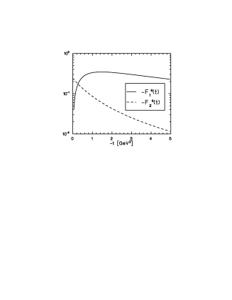
Figure 5: Strange ffs based on the approach with maximal OZI violation.

Of particular interest is the onset of pQCD. Only for $G_{M}^{p}(t)$ data for $Q^{2}>10$ GeV² exist. While these data are consistent with the pQCD scaling $L^{-1}(Q^{2})Q^{4}G_{M}^{p}(Q^{2})\to\,\,$constant, where $L^{-1}(Q^{2})$ accounts for the leading logs, they are not precise enough to rule out a non–scaling behaviour, compare Fig.5 in ref.[11]. Also shown in that figure is the same quantity without the log corrections. All data for the much discussed quantity $Q^{2}F_{2}^{p}(Q^{2})/F_{1}^{p}(Q^{2})$ are below $Q^{2}=10$ GeV² which in our approach is still in the hadronic region since $\Lambda^{2}\simeq 10$ GeV² for the best fit. Stated differently, the tails of the vector meson poles are still sizeable at $Q^{2}\simeq\Lambda^{2}$ and thus the onset of pQCD can not be expected in this regime.

5 Inclusion of the time–like data

In the time–like region, the form factors can be determined either in $\bar{p}p$ annihilation or in $e^{+}e^{-}\to\bar{p}p,\bar{n}n$ collisions [15]. In particular, the FENICE experiment [16] has for the first time measured the (magnetic) neutron form factor. These data and the corresponding ones for the proton, complemented by the total cross section measurement of $e^{+}e^{-}\to mh$ below the threshold, seem to indicate a narrow structure at $\sqrt{t}=1.85\,$GeV, as discussed in detail by Voci at this workshop [6]. For a comprehensive summary of the status before, see Ref.[17]. It is important to add the following remarks on the extraction of the time–like form factors to be discussed. At the nucleon–anti-nucleon threshold, one has only S–wave production, consequently

$$G_{M}(4m^{2})=G_{E}(4m^{2})\quad.$$ (8)

Furthermore, at large momentum transfer one expects the magnetic form factor to dominate. From the data, one can not separate $|G_{M}|$ from $|G_{E}|$ so one has to make an assumption, either setting $|G_{M}|=|G_{E}|=|G|$ or $|G_{E}|=0$. Most recent data are presented for the magnetic form factors [17] and it thus natural to proceed accordingly in the dispersive analysis, i.e. to fit the magnetic form factors in the time–like region. In fig.3, we show the fit to the available space– and time–like data available before the workshop[18] for $t\leq 6\,$GeV². At larger momentum transfer, the unphysical cut due to the logaritm at $t_{\Lambda}=\Lambda^{2}-Q_{0}^{2}$ starts to distort the time–like ffs. This should be eventually overcome by choosing another function that allows to implement the leading QCD corrections to the power law fall–off of the ffs. These fits are optimized by keeping the masses of two isovector poles on physical values and by letting $\Lambda$ vary. This leads to $\Lambda^{2}=12.0\,$GeV², slightly larger than if one fits the space–like data alone. In that figure, we also show the result with an additional isoscalar pole at 1680 MeV [18]. Clearly, the trend of the proton data can be described, although the sharp rise close to threshold is underestimated. In contrast, the magnitude of the neutron data can not be explained by our three–pole fits. This is further quantified in fig.4. There, one of the isovector poles is forced to be at 1850 MeV and the highest isoscalar one at 1600 MeV. The proton magnetic ff is almost unchanged and the neutron ff still rises with decreasing $t$, in contrast to the trend of the new FENICE data. Interestingly, the electric neutron ff (shown by the dashed line) has a zero close to threshold. It is important to stress that these data are still too scarce and imprecise to have an essential effect on the total $\chi^{2}$ of the fit. Even if one decreases the empirical uncertainties to tiny numbers, the three–pole fit can not be forced to have a vanishing neutron form factor at the nucleon–anti-nucleon threshold. Finally, I mention that the values for the nucleon radii and meson couplings given above are not affected by the inclusion of the time–like data. For a more phenomenological approach, see ref.[19].

Figure 3: Fit to the space– and time-like data with three (solid lines) and four (dashed lines) isoscalar poles as described in the text.

Figure 4: Fit to the space– and time-like data with three is/iv poles. One isovector pole fixed at 1.85 GeV as described in the text. Dashed lines: Electric ff.

6 Strangeness in the nucleon

The isoscalar electromagnetic ffs contain some information about the matrix elements of the strange vector current $\bar{s}\gamma_{\mu}s$ in the nucleon. This is most easily seen in the vector dominance model, where one has a photon–hadron coupling mediated by the $\phi$ meson, which is almost entirely an $\bar{s}s$ state. On the other hand, the OZI rule lets one expect that such a contribution is small since the nucleon is made of non–strange constituent quarks. In the following, I will discuss two very different approaches. The first one amounts to a strong violation of the OZI rule whereas in the second, this rule is respected. The corresponding strange matrix elements are very different in size, showing that we have not yet reached a very deep theoretical understanding of this issue.

6.1 Maximal OZI violation

The large $\phi$ meson coupling to the nucleon given in eq.(7) was already observed in the fits of the Karlsruhe–Heksinki group and the consequences concerning the validity of the OZI rule were discussed in [20]. Jaffe [21] has shown how one can get bounds on the strange vector form factors in the nucleon from such dispersion theoretical results. It amounts to separating the strangeness contribution from the three isoscalar poles. For the $\omega$ and the $\phi$, this is done naturally by observing that there is a small mixing angle with respect to the nonet flavor eigenstates. The strangeness component of the third pole is fixed by demanding normalization conditions like $F_{1}^{s}(0)=0$ and conditions on the large momentum fall-off of $F_{1,2}^{s}(t)$ as $t\to-\infty$. The main assumption of this approach is that these strange form factors have the same large–$t$ behaviour as the non–strange isoscalar ones. If the fall–off for the strange form factors is faster, the strange matrix elements will be reduced. Using the best fit together with a better treatment of the symmetry breaking in the vector nonet, it is straightforward to update Jaffe’s analysis. One finds for the strange magnetic moment and the strangeness radius [22] (see also ref.[23]),

$$\mu_{s}=-0.24\,\,{\rm n.m.}\,,\,\,\,r_{s}^{2}=0.17\ldots 0.21\,\,{\rm fm}^{2}\,,$$ (9)

for the fit with the third isoscalar pole at 1.42 GeV (smaller value) and at 1.6 GeV (larger value for the strange radius). The value for $\mu_{s}$ is stable. Furthermore, the strange ff $F_{2}^{s}(t)$ follows a dipole with a cut–off mass of 1.46 GeV, $F_{2}^{s}(t)=\mu_{s}/(1-t/2.41\,{\rm GeV}^{2})^{2}$. The corresponding strange ffs are shown in fig.6. It is important to stress that these numbers should be considered as upper bounds. Such a strongly coupled $\phi$ meson subsumes other effects like the strong $\pi\rho$ correlations and it is therefore mandatory to consider an alternative scenario, in which strength is moved from the $\phi$.

6.2 OZI resurrected

The $\phi$ meson has a sizeable branching fraction into the $\pi\rho$ final state. Furthermore, it is well known that in meson exchange models there is an important contribution from the $\pi\rho$ continuum to the 3–pion ($\omega$) exchange. In the Bonn–Jülich Potential, this contribution has been calculated in ref.[24]. There, a parametrization of the corresponding $\pi\rho$ spectral function with a mass of $M_{\omega^{\prime}}=1.22\,$GeV and fixed coupling constants was given. This approach has further been extended to include kaon loops and hyperon excitations, with the parameters fixed from a study of the reactions $p\bar{p}\to\Lambda\bar{\Lambda}$ and $p\bar{p}\to\Sigma\bar{\Sigma}$. There are sizeable cancellations between the various contributions from graphs with intermediate $K$’s, $K^{*}$’s and diagrams with the direct hyperon interactions [25] leading to a very small $\phi$ coupling,

$$\frac{g_{\phi NN}^{2}}{4\pi}\simeq 0.005\,,\,\,\,\kappa_{\phi}\simeq\pm 0.2\,\,.$$ (10)

The sign of the tensor coupling is very sensitive to the details of the calculation. Neglecting the $\omega\,\phi$ mixing, one can now perform a fit with the OZI rule imposed. For that, one takes the poles corresponding to the $\pi\rho$ continuum and the $\omega$ and $\phi$ mesons with fixed couplings given by the model and has as remaining free parameters the mass of the fourth isoscalar pole ($M_{S}$), the strength $a_{1}^{S}$ and the mass of the third isovector pole. The other parameters are constrained as described before (normalizations, superconvergence relations etc). It is important to stress that one has to include a fourth isoscalar pole so as to be able to fulfill all these constraints. The corresponding strange form factors take the form [26]

$$F_{1}^{s}(t)=t\,L(t)\,a_{1}^{\phi}L_{\phi}^{-1}\,\frac{M_{\phi}^{2}-M_{S}^{2}}{(t-M_{\phi}^{2})(t-M_{S}^{2})}\,,\,\,F_{2}^{s}(t)=L(t)\,a_{2}^{\phi}L_{\phi}^{-1}\,\frac{M_{\phi}^{2}-M_{S}^{2}}{(t-M_{\phi}^{2})(t-M_{S}^{2})}\,,\,\,$$ (11)

imposing the same large-$t$ constraints as for the isoscalar ffs and $L_{\phi}^{-1}=1/L(M_{\phi}^{2})$. Clearly, the size of these strange ffs is given by the strength of the $\phi$–nucleon couplings (as encoded in the residua $a_{1,2}^{\phi}$). For a typical set of coupling constants, we find (for a more detailed account, see ref.[26])

$$\mu_{s}=0.003\,\,{\rm n.m.}\,,\,\,\,r_{s}^{2}=0.002\,\,{\rm fm}^{2}\,,$$ (12)

which are two orders of magnitude smaller than the numbers based on the ansatz with maximal OZI violation. The corresponding strange ffs are shown in fig.6. Including the $\omega\,\phi$ mixing would lead to somewhat larger values but not change the conclusion that the extraction of the strange vector current matrix elements from a dispersion-theoretical fit to the em ffs hinges strongly on whether one views the $\phi$ as an isolated pole with a large effective coupling or whether one shifts a large amount of the strength from the region around $t\simeq 1\,$GeV² into a pole that parametrizes the strong $\pi\rho$–correlations seen in the analysis of the NN interaction.

Figure 6: Strange ffs based on the approach with the OZI rule imposed. Notice the different y-scale compared to fig.5.

6.3 Strangeness and unitarity

A different approach to get bounds on the matrix elements of the strange vector current $\bar{s}\gamma_{\mu}s$ has been discussed in ref.[27]. Dispersion relations are used to study the contribution from the $\bar{K}K$ intermediate state to the ff spectral functions. As expected, a direct calculation shows that using the $K\bar{K}\to N\bar{N}$ amplitudes in the Born (tree) approximation in the dispersion relations is equivalent to a one-loop calculation within the effective field theory approach. For the latter, the SU(3) non–linear $\sigma$ model is chosen. A serious violation of unitarity is found if one translates the bounds on the helicity amplitudes for the $KN$ scattering amplitude into bounds for the spectral functions. This means that resonant and non–resonant kaon rescattering (or higher loop effects) can not be neglected in such type of analysis. This agrees with the findings of the model discussed in the previous paragraph. Furthermore, it is pointed out in [27] that the effect of the strange kaon ff defined via

$$\langle 0|\bar{s}\gamma_{\mu}s|K^{-}(k_{1})K^{+}(k_{2})\rangle=(k_{1}-k_{2})_{\mu}\,F^{s}_{K}(t)\,\,\,,$$ (13)

is non–negligible if e.g. $F^{s}_{K}(t)$ is modelled by a Gounaris–Sakurai form peaked around the mass of the $\phi$. A refined analysis which uses the empirical information on $KN\to KN$ or $K\bar{K}\to N\bar{N}$ data continued appropriately to get more stringent bounds on the strange radius and magnetic moment is possible but not yet available.

7 Outlook

To my opinion, there are three major issues to be resolved.

• Better and more consistent data in the space–like region for low, intermediate and large momentum transfer are necessary to further sharpen the values of the nucleon radii and vector meson coupling constants. This is an experimental problem. The feasibility of improving upon the existing data basis is discussed in Klein’s talk [14].

• More theoretical work is needed to get a better handle on the matrix elements of the strange vector current, as exemplified in Sec. 6 by the approach which accounts for the strong $\pi\rho$ correlations and the bounds from unitarity. A deeper theoretical understanding is necessary for setting the stage for the strange form factor measurements at TJNAF.

• The neutron ffs in the time–like region have to be measured more precisely close to the nucleon–anti-nucleon threshold. If the interesting structure indicated by the FENICE data persists, theory is challenged to explain it. This might finally be the trace of the much searched for dibaryon states.

Finally, it is important to stress that all these problems are intertwined. For example, the extraction of the strange ffs from parity–violation experiments can only be done precisely if the data are accurate enough but also the non–strange ffs are known precisely, since in most parity–violation experiments the latter are used as amplification factors.

References

- [1] M. Weitz et al., Phys. Rev. Lett. 72 (1994) 328; D.J. Berkeland et al., Phys. Rev. Lett. 75 (1995) 2470
- [2] W.R. Frazer and F.J. Fulco, Phys. Rev. Lett. 2 (1959) 365; Phys. Rev. 117 (1960) 1609
- [3] Y. Nambu, Phys. Rev. 106 (1957) 1366
- [4] J.J. Sakurai, Ann. Phys. (NY) 11 (1960) 1
- [5] S.J. Brodsky and G. Farrar, Phys. Rev. D11 (1975) 1309
- [6] C. Voci, these proceedings; R. Baldini, private communication
- [7] J. Gasser, M.E. Sainio and A. varc, Nucl. Phys. B307 (1988) 779
- [8] V. Bernard, N. Kaiser and Ulf-G. Meißner, [hep-ph/9607428], Nucl. Phys. A, in print
- [9] S. Kopecky et al., Phys. Rev. Lett. 74 (1995) 2427
- [10] L. Magnea and G. Sterman, Phys. Rev. D42 (1990) 4222
- [11] P. Mergell, Ulf-G. Meißner and D. Drechsel, Nucl. Phys. A596 (1996) 367
- [12] G. Höhler et al., Nucl. Phys. B114 (1976) 505
- [13] S. Platchkov et al., Nucl. Phys. A510 (1990) 740
- [14] F. Klein, these proceedings
- [15] M. Castellano et al., Nuovo Cim. A14 (1973) 1; G. Bassompierre et al., Phys. Lett. B64 (1976) 475, B68 (1977) 477, Nuovo Cim. A73 (1983) 347; B. Delcourt et al., Phys. Lett. B86 (1979) 395; D. Bisello et al., Nucl. Phys. B224 (1983) 379; G. Bardin et al., Phys. Lett. B255 (1991) 149; B257 (1991) 514; Nucl. Phys. B411 (1994) 3
- [16] A. Antonelli et al., Phys. Lett. B313 (1993) 283; B334 (1994) 431
- [17] R. Baldini and E. Pasqualucci, in ”Chiral Dynamics: Theory and Experiment”, A.M. Bernstein and B.R. Holstein (eds.), Springer, Heidelberg, 1995
- [18] H.–W. Hammer, Ulf-G. Meißner and D. Drechsel, Phys. Lett. B385 (1996) 343
- [19] Z. Dziembowski and A. Szczurek, Phys. Lett. B387 (1996) 875
- [20] H. Genz and G. Höhler, Phys. Lett. B61 (1976) 389
- [21] R.L. Jaffe, Phys. Lett. B229 (1989) 275
- [22] H.–W. Hammer, Ulf-G. Meißner and D. Drechsel, Phys. Lett. B367 (1996) 323
- [23] H. Forkel, preprint ECT*/Sept/014-95, 1995
- [24] G. Janßen, Dissertation, University of Bonn, 1995
- [25] V. Mull, Dissertation, University of Bonn, 1996
- [26] Ulf-G. Meißner, J. Speth and W. van Orden, in preparation
- [27] M. Musolf, H.–W. Hammer and D. Drechsel, preprint [hep-ph/9610402]