Abstract

Using a known result by Falk et al. for the $1/m_{b}^{2}$ correction to the dilepton invariant mass spectrum in the decay $B\rightarrow X_{s}\,\mu^{+}\mu^{-}$, we calculate the $1/m_{b}^{2}$ correction to the left-right muon polarization asymmetry in this decay. Employing an up-to-date range of values for the non-perturbative parameter $\lambda_{1}$, we find that the correction is much smaller than it should have been expected from the previous work by Falk et al.

To appear in Physical Review D.

Introduction

Rare decays of $B$ mesons have been studied extensively in the last few years. Such decays are forbidden in the tree-level approximation and proceed through loop diagramms only. Consequently, they are sensitive to the complete particle content of a given theory and their analysis may thus shed some light on possible new physics beyond the standard model (SM). In this paper, we focus on the inclusive decay $B\rightarrow X_{s}\,\mu^{+}\mu^{-}$, where $X_{s}$ denotes an arbitrary hadronic final state with total strangeness $-1$. In contrast to the decay $B\rightarrow X_{s}\,\gamma$, the three-body decay $B\rightarrow X_{s}\,\mu^{+}\mu^{-}$ allows one to define and measure several kinematic distributions. Beside the invariant mass spectrum of the lepton pair a forward-backward charge asymmetry [1] and a left-right polarization asymmetry [2, 3] have been proposed. The simultaneous measurement of these distributions allows one to extract the values of the Wilson coeffients which govern the decay amplitude and contain the short distance physics [4]. The values of these Wilson coefficients are sensitive to new physics and in a measurement of the kinematic distributions one might be able to detect deviations from the SM prediction. For this reason the distributions mentioned above should be calculated as precise as possible.

Meanwhile a complete next-to-leading order (NLO) calculation of the relevant Wilson coefficients is available [5, 6]. These coefficients properly include the short distance QCD effects and the NLO approximation considerably reduces the (otherwise significant) theoretical uncertainty in the final result which stems from its dependence on the renormalization scale.

Apart from these perturbative calculations which rely entirely on the spectator model (defined as the free quark decay model including perturbative QCD), long distance effects due to the non-perturbative physics at low scales have to be taken into account. Important corrections are first of all generated by intermediate $c\bar{c}$ bound states (e. g. the channel $b\rightarrow s\,J/\psi\rightarrow s\mu^{+}\mu^{-}$) which influence the kinematic distributions even far away from the resonance region. For a way to deal with these effects we refer to the literature [7, 8, 9, 10].

Additionally, there are non-perturbative effects due to the binding of the $b$ quark inside the $B$ meson. It is strongly expected that for inclusive decays of heavy quarks such effects may be incorporated by a controlled expansion in inverse powers of the mass of the decaying quark, the so-called heavy quark expansion (HQE) [11, 12]. The first term of this expansion can be shown to reproduce the spectator model. Falk, Luke and Savage [14] calculated the first non-vanishing – i. e. $O(1/m_{b}^{2})$ – correction to the dilepton invariant mass spectrum in the decay $B\rightarrow X_{s}\,\mu^{+}\mu^{-}$ some time ago.

It is this type of corrections we are dealing with in the following. We slightly extend the work of Liu and Delbourgo [3] about the left-right polarization asymmetry by presenting the $1/m_{b}^{2}$ correction to this distribution. It should particularly be stressed that in the numercial analysis we take into account a present range of values for $\lambda_{1}$ (one of the non-perturbative parameters that occur by performing the HQE), and that these values differ drastically from the one used in Ref. [14].

The left-right asymmetry

The general framework for decays like $B\rightarrow X_{s}\,\mu^{+}\mu^{-}$ is the effective theory approach with the effective Hamiltonian as the central element. Once the effective Hamiltonian is given one can calculate the decay amplitude and the kinematic distributions mentioned above. The effective Hamiltonian for the decay $B\rightarrow X_{s}\,\mu^{+}\mu^{-}$ has been calculated in the NLO approximation by Misiak [5] and independently by Buras and Münz [6]. In our paper we entirely use the notation introduced in Ref. [6] and we refer to this paper for the operator basis, the analytic expressions of the Wilson coefficients and for the details concerning the NLO calculation.

Let us now consider the left-right asymmetry. It is defined as

$$\frac{dA^{LR}}{d\hat{s}} = \frac{d\Gamma^{L}}{d\hat{s}}-\frac{d\Gamma^{R}}{d\hat{s}},$$

where

$$\hat{s} = \frac{(p_{\mu^{+}}+p_{\mu^{-}})^{2}}{m_{b}^{2}}$$

is the scaled 4-momentum transfer to the muons and $d\Gamma^{L}/d\hat{s}$  ($d\Gamma^{R}/d\hat{s}$) denotes the invariant mass spectrum for a decay into purely left-handed (right-handed) muons. Instead of calculating $d\Gamma^{L}/d\hat{s}$ and $d\Gamma^{R}/d\hat{s}$ separately, $dA^{LR}/d\hat{s}$ can alternatively be obtained directly from the invariant mass spectrum $d\Gamma/d\hat{s}$. With the operator basis used in Ref. [6], $d\Gamma/d\hat{s}$ is derived in terms of the Wilson coefficients $C_{9}$ and $C_{10}$. The corresponding operator $Q_{9}$ contains a vector coupling of the muons, $Q_{10}$ an axial-vector coupling. Defining a left-handed and a right-handed operator by

$$Q_{L} = Q_{9}-Q_{10},$$

$$Q_{R} = Q_{9}+Q_{10},$$

one obtains $d\Gamma/d\hat{s}$ in terms of the corresponding Wilson coefficients $C_{L}$ and $C_{R}$ by the simple substitution

$$C_{9} = C_{L}+C_{R},$$

$$C_{10} = C_{R}-C_{L}.$$

Since the remaining operators $Q_{1}\cdots Q_{8}$ contain only vector couplings to the muons, one finds in this basis

$$\frac{dA^{LR}}{d\hat{s}} = \left.\frac{d\Gamma}{d\hat{s}}\right|_{C_{R}=0}-\left.\frac{d\Gamma}{d\hat{s}}\right|_{C_{L}=0}.$$

The final result may be transformed back to the basis $Q_{9}$, $Q_{10}$ and re-expressed in terms of $C_{9}$ and $C_{10}$. Following these steps one reproduces the result for the left-right asymmetry in Ref. [3] if one starts with the invariant mass spectrum as given in Ref. [6]. Keeping this procedure in mind one can extract the $1/m_{b}^{2}$-correction to the left-right asymmetry from the $1/m_{b}^{2}$-correction to the invariant mass spectrum given in [14]. We stress that it is not necessary to repeat the full calculation Falk et al. have done in order to find the $1/m_{b}^{2}$-correction for the left-right asymmetry. We obtain

$$\frac{dA^{LR}}{d\hat{s}} = \frac{dA_{0}^{LR}}{d\hat{s}}\,+\,\frac{dA_{2}^{LR}}{d\hat{s}},$$

$$\frac{dA_{0}^{LR}}{d\hat{s}} = -\,\frac{\Gamma(b\rightarrow cl^{-}\overline{\nu})}{f(z)\cdot\kappa(z)}|V_{tb}|^{2}\,\left|\frac{V_{ts}}{V_{cb}}\right|^{2}\,\frac{\alpha^{2}}{2\pi^{2}}\,(1-\hat{s})^{2}\tilde{C}_{10}\left[(1+2\hat{s})\mbox{Re}\left(\tilde{C}_{9}^{eff}\right)\,+\,6\,C_{7}^{(0)eff}\right],$$

$$\frac{dA_{2}^{LR}}{d\hat{s}} = -\,\frac{\Gamma(b\rightarrow cl^{-}\overline{\nu})}{f(z)\cdot\kappa(z)}|V_{tb}|^{2}\,\left|\frac{V_{ts}}{V_{cb}}\right|^{2}\,\frac{\alpha^{2}}{2\pi^{2}}\,(1-\hat{s})\tilde{C}_{10}\left(k_{1}^{LR}(\lambda_{1},\hat{s})+k_{2}^{LR}(\lambda_{2},\hat{s})\right),$$

where we defined $z=m_{c}/m_{b}$ and

$$k_{1}^{LR}(\lambda_{1},\hat{s}) = \frac{\lambda_{1}}{2m_{b}^{2}}\left\{\left(-2\hat{s}^{2}+3\hat{s}+5\right)\mbox{Re}\left(\tilde{C}_{9}^{eff}\right)-2(3\hat{s}-5)C_{7}^{(0)eff}\right\},$$

$$k_{2}^{LR}(\lambda_{2},\hat{s}) = \frac{\lambda_{2}}{2m_{b}^{2}}\left\{3\left(-10\hat{s}^{2}+15\hat{s}+1\right)\mbox{Re}\left(\tilde{C}_{9}^{eff}\right)-6(7\hat{s}-5)C_{7}^{(0)eff}\right\}.$$

$dA_{0}^{LR}/d\hat{s}$ denotes the spectator model result. It agrees with the result in Ref. [3]. The functions $f(z)$ and $\kappa(z)$ are the phase-space factor and the one gluon correction to the decay $b\rightarrow ce\bar{\nu}$ given in Eqn. (2.31) and (2.32) of Ref. [6]. The Wilson coefficients $C_{7}^{(0)eff},\,\tilde{C}_{9}^{eff}\mbox{and }\tilde{C}_{10}$ are also defined in Ref. [6], Eqn. (2.3), (2.28) and (2.8). Note that the effective coefficient $\tilde{C}_{9}^{eff}$ depends explicitely on $\hat{s}$ because it contains the influence of the operators $Q_{1}\cdots Q_{6}$. Finally, $dA_{2}^{LR}/d\hat{s}$ denotes the $1/m_{b}^{2}$-correction, given in terms of the two HQET parameter $\lambda_{1}$ and $\lambda_{2}$. A definition of them as matrix elements can be found in Ref. [14], Eq. (2.21).

Numerics

Let us now examine the size of the correction compared with the spectator model result. In doing this we do not incorporate the long distance effects due to intermediate $c\bar{c}$ resonances. We do not neglect them because they are small – in fact, as already mentioned, they do have a large effect on the shape of the spectra even far away from the resonance region. The common way to deal with these resonances is a simple replacement of $\tilde{C}_{9}^{eff}$ by $\tilde{C}_{9}^{eff}+\mbox{Res($\hat{s}$)}$ (see e. g. Ref. [10]), where the function Res$(\hat{s})$ is chosen to produce resonance peaks at the masses of the intermediate $c\bar{c}$ bound states. The relative correction to the spectator model, however, is nearly the same with or without this replacement of $\tilde{C}_{9}^{eff}$. So, for simplicity, we show the non-resonant results only.

In the appendix we give a list of the numerical values of all input parameter we used. Some remarks should be made concerning the non-perturbative parameter $\lambda_{1}$ and $\lambda_{2}$. From the $B\,-\,B^{*}$ mass splitting the numerical value of $\lambda_{2}$ is well known to be 0.12$\,\mbox{GeV}^{2}$ [15]. $\lambda_{1}$ is much less understood. In Ref. [14] $\lambda_{1}=0.5\,\mbox{GeV}^{2}$ was used in the numerical analysis. These values led to an enhancement of roughly 10 percent over the full range of $\hat{s}$ in the invariant mass spectrum. This value of $\lambda_{1}$, however, is no longer appropriate. Even if there is still some controversary about the magnitude, the sign of $\lambda_{1}$ is strongly believed to be negative. There have been attempts to calculate $\lambda_{1}$ using QCD sum rules [16, 17, 18, 19] and, alternatively, to extract it by a fit to the data from $B$ and $D$ decays [20, 21]. Even an upper bound has been proposed [22, 23, 24]. However, the values found lie in the range $-0.6\,\mbox{GeV}^{2}\leq\,\lambda_{1}\,\leq\,-0.1\,\mbox{GeV}^{2}$, which is quite large.

In Fig. 1 we plot the spectator model prediction with and without the $1/m_{b}^{2}$ correction.

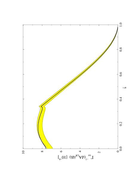
Figure 1: The left-right asymmetry in the decay $B\rightarrow X_{s}\mu^{+}\mu^{-}$ (normalized to the total decay width of the $B$ meson). The solid line represents the spectator model result. The shaded area corresponds to the left-right asymmetry including the $1/m_{b}^{2}$ correction, varying $\lambda_{1}$ between $-0.6\,\mbox{GeV}^{2}$ and $-0.1\,\mbox{GeV}^{2}$. The upper edge of the area is given by $\lambda_{1}\,=\,-0.1\,\mbox{GeV}^{2}$, the lower edge by $\lambda_{1}\,=\,-0.6\,\mbox{GeV}^{2}$.

The influence of the correction never exceeds a rate of 3.5% in the high $\hat{s}$-region $(\hat{s}\geq 0.4)$ and maximally reduces the spectrum by 9.5% for very small values of $\hat{s}$. We emphasize that the smallness of the correction is due to an accidental cancellation of the corrections $k_{1}^{LR}$ and $k_{2}^{LR}$. With $\lambda_{1}\approx-3\,\lambda_{2}$ the functions $k_{1}^{LR}$ and $k_{2}^{LR}$ almost cancel in the high $\hat{s}$ region. For the integrated left-right asymmetry the correction lies between +3% and –5% compared to the spectator model result.

This small correction in mind it is interesting to show again the $1/m_{b}^{2}$ correction to the invariant mass distribution with negative values of $\lambda_{1}$. This is done in Fig. 2.

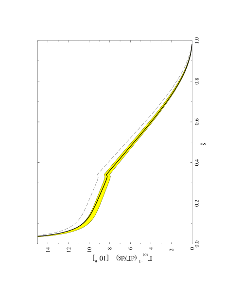
Figure 2: The dilepton invariant mass spectrum in the decay $B\rightarrow X_{s}\mu^{+}\mu^{-}$ (normalized to the total decay width of the $B$ meson). The solid line represents the spectator model result. The shaded area corresponds to the spectrum including the $1/m_{b}^{2}$ correction, varying $\lambda_{1}$ between $-0.6\,\mbox{GeV}^{2}$ and $-0.1\,\mbox{GeV}^{2}$. As in Fig. 1 the upper edge of the area is given by $\lambda_{1}\,=\,-0.1\,\mbox{GeV}^{2}$, the lower edge by $\lambda_{1}\,=\,-0.6\,\mbox{GeV}^{2}$. The dashed line is the result obtained by Falk et al. using $\lambda_{1}=0.5\,\mbox{GeV}^{2}$.

The overall correction is significantly reduced compared to the result in Ref. [14]. As in the case for the left-right asymmetry, the correction to the spectator model is at most 3.5% for $\hat{s}\geq 0.4$ and maximally differs by 5.2% near $\hat{s}=0.1$. The correction results in a maximal decrease of the integrated spectrum of 3.8% for $\lambda_{1}=-0.6\,\mbox{GeV}^{2}$. In comparison, the integrated spectrum increases by 9.3% taking $\lambda_{1}$ as high as the value used in Ref. [14].

As long as $\lambda_{1}$ is poorly known, the following numerical formulae might be useful. They describe the relative size of the $1/m_{b}^{2}$ correction to the spectator model results of the integrated left-right asymmetry and the branching ratio:

$$\frac{\Delta A^{LR}}{A^{LR}_{0}} = \left(\left[\frac{\lambda_{1}}{\mbox{GeV}^{2}}\right]\,+\,0.28\right)\times 15.3\,\%\,,$$

$$\frac{\Delta{\cal B}[B\rightarrow X_{s}\mu^{-}\mu^{+}]}{{\cal B}[B\rightarrow X_{s}\mu^{-}\mu^{+}]_{0}} = \left(\left[\frac{\lambda_{1}}{\mbox{GeV}^{2}}\right]\,+\,0.28\right)\times 12.0\,\%\,.$$

Note that the $1/m_{b}^{2}$ correction depends linearly on $\lambda_{1}$, therefore these formulae are valid for all values of $\lambda_{1}$. They also imply that for $\lambda_{1}=-0.28\,\mbox{GeV}^{2}$ (and $\lambda_{2}=0.12\,\mbox{GeV}^{2}$) one obtains the spectator model results

$$\Gamma_{tot}^{-1}\,A_{0}^{LR} = 4.74\times 10^{-6},$$

$${\cal B}[B\rightarrow X_{s}\mu^{-}\mu^{+}]_{0} = 6.03\times 10^{-6}.$$

It is instructive to compare the size of the $1/m_{b}^{2}$ correction to the left-right asymmetry with that of other unkown corrections or uncertainties preventing a precise theoretical prediction of this quantity. We looked at various sources of uncertainties, a complete list of the corresponding errors is given in Table 1.

Uncertainty due to …	$\Delta A^{LR}/A^{LR}_{0}$	$\Delta{\cal B}/{\cal B}$
long-distance effects	$+15\%$	+10%
$m_{b}/2<\mu<2m_{b}$	$\pm 8\%$	$\pm 2\%$
$m_{t}=(167\pm 6)\,{\rm GeV}$	$\pm 6\%$	$\pm 7\%$
$m_{c}=(1.4\pm 0.1)\,{\rm GeV}$	$\pm 6\%$	$\pm 6\%$
${\cal B}[B\rightarrow X_{c}l^{-}\overline{\nu}]$	$\pm 4.8\%$	$\pm 4.8\%$
$|V_{ts}/V_{cb}|^{2}=0.95\pm 0.04$	$\pm 4.2\%$	$\pm 4.2\%$
$\alpha_{s}(M_{Z})=0.118\pm 0.003$	$\pm 1.5\%$	$\pm 0.2\%$
$m_{b}=(4.8\pm 0.3)\,{\rm GeV}$	$\pm 0.7\%$	$\pm 1.1\%$
$m_{s}=(0.1\pm 0.1)\,{\rm GeV}$	$\pm 0.7\%$	$\pm 0.6\%$

Table 1: Various sources of uncertainty for the integrated left-right asymmetry as well as for the total branching ratio of the decay $B\rightarrow X_{s}\mu^{+}\mu^{-}$, in order of their numerical importance. For the first two entries, see the explanations in the text.

The most important error stems from the lack of the next-to-next-to-leading order QCD calculation. This truncation of the perturbative series manifests itself in the renormalization scale dependence of the spectra and integrated rates. By varying the renormalization scale $\mu$ between $m_{b}/2$ and $2m_{b}$ (i. e. in such a manner that $\ln m_{b}/\mu$ remains small) we estimated the corresponding uncertainty to be about $\pm 8\%$. Apart from this we have to cope with our insufficient knowledge of the masses of the top and charm quark, which enter through loop diagrams and the phase-space factor $f(z)$. Both of these masses give rise to an uncertainty of roughly $\pm 6\%$. The errors due to the CKM matrix elements and the semileptonic branching ratio are not large, but also comparable to the $1/m_{b}^{2}$ correction. The other inaccurate known paramters, including $\alpha_{s}(M_{Z})$ and the masses of the remaining quarks, affect the left-right asymmetry only by a small amount (i. e. not more than $\pm 1\%$). Apart from these rather trivial dependences on the parameters, there remains one potential systematic error, namely the long-distance contributions due to $c\bar{c}$-resonances. Modelling the resonances as in Ref. [10], we estimated them to enlarge the left-right asymmetry by roughly 15% (whereby this number depends to some extent on the applied experimental cuts). In the worst case, lacking anything better, the associated error should be taken to be in the same order of magnitude than the correction itself, albeit we would call this a very conservative and perhaps unnecessary pessimistic view.

The numbers of Table 1 show that the $1/m_{b}^{2}$ corrections are numerically not very significant compared to all the other uncertainties presently existing. However, two remarks should be made. On the one hand, we would have arrived at a much larger correction of about 10% if we had used the old value $\lambda_{1}=0.5\,{\rm GeV}^{2}$ as in Ref. [14] (which was published only three years ago). It is interesting to note that at the moment most experimental and theoretical developments are in favour of the assumption that the $1/m_{b}^{2}$ corrections are generically small. On the other hand, the $1/m_{b}^{2}$ corrections are quantities of principle interest. Assuming the validity of the HQE, there existence is a fundamental and predictable property of QCD. So they should be calculated indepently of their actual size (which, of course, is by no means known a priori). Even if today the overall error is dominated by the uncertainties in the SM parameters, one cannot say how this picture will change during the forthcoming years.

Summary

In this brief note we presented the nonperturbative $1/m_{b}^{2}$ correction to the left-right asymmetry for the rare decay $B\rightarrow X_{s}\,\mu^{+}\mu^{-}$. With a present range of values for the parameter $\lambda_{1}$ we found a correction as small as roughly four percent for the integrated left-right asymmetry. We also showed the invariant mass spectrum with these new values for $\lambda_{1}$ and found the correction significantly smaller than in Ref. [14].

Note added in proof

After completion of this work a recalculation [25] of the $1/m_{b}^{2}$-correction to the decay $B\rightarrow X_{s}\,\mu^{+}\mu^{-}$ appeared. The authors of Ref. [25] use the same method as Falk, Luke and Savage [14] but obtain a different result. If Ref. [25] should be confirmed, our numerical results would of course change.

Appendix: Input parameter

$m_{b}=4.8\,\mbox{GeV}$, $m_{c}=1.4\,\mbox{GeV}$, $m_{s}=0.1$, $m_{\mu}=0$, $m_{t}=167\,\mbox{GeV}$, $M_{W}=80.2\,\mbox{GeV}$, $\mu=5\,\mbox{GeV}$, $\left|V_{tb}\right|=1$, $\left|V_{ts}/V_{cb}\right|=0.95$, $\sin^{2}\theta_{W}=0.23$, $\alpha=\alpha(M_{Z})=1/129$, $\alpha_{s}(M_{Z})=0.118$, ${\cal B}(B\rightarrow X_{c}l^{-}\bar{\nu})=0.105$, $\lambda_{2}=0.12\,\mbox{GeV}^{2}$, $-0.6\,\mbox{GeV}^{2}\leq\lambda_{1}\leq-0.1\,\mbox{GeV}^{2}$ (see text).

References

- [1] A. Ali, T. Mannel, and T. Morozumi, Phys. Lett. B273 (1991) 505.
- [2] J. Hewett, Phys. Rev. D53 (1996) 4964.
- [3] D. Liu and R. Delbourgo, Phys. Rev. D53 (1996) 548.
- [4] A. Ali, G. F. Guidice, and T. Mannel, Z. Phys. C67 (1995) 417.
- [5] M. Misiak, Nucl. Phys. B393 (1993) 23, ibid. B439 (1995) 461E.
- [6] A. J. Buras and M. Münz, Phys. Rev. D52 (1995) 186.
- [7] C. S. Lim, T. Morozumi, and A. I. Sanda, Phys. Lett. B218 (1989) 343.
- [8] N. G. Deshpande, J. Trampetić, and K. Panose, Phys. Rev. D39 (1989) 1461.
- [9] P. O’Donnel and H. K. K. Tung, Phys. Rev. D43 (1991) R2067.
- [10] F. Krüger and L. M. Sehgal, Phys. Lett. B380 (1996) 199.
- [11] J. Chay, H. Georgi, and B. Grinstein, Phys. Lett. B247 (1990) 399.
- [12] I. Bigi, N. Ultrasev, and A. Vainstein, Phys. Lett. B293 (1992) 430, ibid. B297 (1993) 477E.
- [13] B. Chibisov, R. D. Dikeman, M. Shifman, and N. Uraltsev, preprint TPI-MINN-96-05-T, hep-ph/9605465.
- [14] A. F. Falk, M. Luke, and M. J. Savage, Phys. Rev. D49 (1994) 3367.
- [15] M. Neubert, Phys. Rep. 245 (1994) 259.
- [16] M. Neubert, Phys. Rev. D46 (1992) 1076.
- [17] V. Eletskii and E. Shuryak, Phys. Lett. B276 (1992) 191.
- [18] P. Ball and V. M. Braun, Phys. Rev. D49 (1994) 2472.
- [19] M. Neubert, preprint CERN-TH/96-208, hep-ph/9608211 .
- [20] A. F. Falk, M. Luke, and M. J. Savage, Phys. Rev. D53 (1996) 6316.
- [21] M. Gremm, A. Kapustin, Z. Ligeti, and M. B. Wise, Phys. Rev. Lett. 77 (1996) 20.
- [22] I. I. Bigi, M. A. Shifman, N. G. Uraltsev, and A. L. Vainshtein, Int. J. Mod. Phys. A9 (1994) 2467.
- [23] I. I. Bigi, M. A. Shifman, N. G. Uraltsev, and A. L. Vainshtein, Phys. Rev. D52 (1995) 196.
- [24] A. Kapustin, Z. Ligeti, M. B. Wise, and B. Grinstein, Phys. Lett. B375 (1996) 327.
- [25] A. Ali, G. Hiller, L. T. Handoko, and T. Morozumi, preprint DESY 96-206, hep-ph/9609449.