Abstract

A quantum-kinetic formulation of the dynamical evolution of a high-energy non-equilibrium gluon system at finite density is developed, to study the interplay between quantum fluctuations of high-momentum (hard) gluons and the low-momentum (soft) mean color-field that is induced by the collective motion of the hard particles. From the exact field-equations of motion of QCD, a self-consistent set of approximate quantum-kinetic equations are derived by separating hard and soft dynamics and choosing a convenient axial-type gauge. This set of master equations describes the momentum space evolution of the individual hard quanta, the space-time development of the ensemble of hard gluons, and the generation of the soft mean-field by the current of the hard particles. The quantum-kinetic equations are approximately solved to order $g^{2}(1+g\overline{A})$ for a specific example, namely the scenario of a high-energy gluon beam along the lightcone, demonstrating the practical applicability of the approach.

I INTRODUCTION AND SUMMARY

The physics of high-density QCD becomes an increasingly popular object of research, both from the experimental, phenomenological interest, and from the theoretical, fundamental point of view. Presently, and in the near future, the collider facilities HERA ($ep$, $eA$?), Tevatron ($p\bar{p}$, $pA$), RHIC and LHC ($p\bar{p}$, $AA$) are able to probe new regimes of dense quark-gluon matter at very small Bjorken-$x$ or/and at large $A$, with rather different dynamical properties. The common feature of high-density QCD matter that can be produced in these experiments, is an expected novel exhibition of the interplay between the high-momentum (short-distance) perturbative regime and the low-momentum (long-wavelength) non-perturbative physics. For example, with HERA and Tevatron experiments, one hopes to gain insight into problems concerning the saturation of the strong rise of the proton structure functions at small Bjorken-$x$, possibly due to color-screening effects that are associated with the overlappping of a large number of small-$x$ partons. Another example is the anticipated formation of a quark-gluon plasma in RHIC and LHC heavy ion collisions, where multiple parton rescattering and cascading may generate a high-density environment, in which the collective motion of the quanta can give rise to non-abelian long-wavelength excitations and screening of color charges.

In any case, the study of coherent low-momentum excitations in QCD, that are generated by, and interacting with, the high-momentum partonic color charges, is of fundamental interest in several respects: Firstly, it provides insight into the basic features of non-abelian multiparticle dynamics and a step towards a rigorous decription of parton transport properties in a dense environment. Secondly, it may help to resolve current problems encountered in perturbative QCD, for instance the absence of static magnetic color-screening [1], the problem of infrared renormalons [2] connected with the resummation of perturbation theory in the small-$x$ regime, or, the problem of confinement associated with collective ‘glue’-behavior of non-perturbative gluons [3]. Interesting progress in these areas is continously being made, and consistent schemes have emerged to perform calculations of the parton evolution at very small-$x$ [4], at very large density [5, 6] and for high-temperature QCD of a quark-gluon plasma [7].

Most progress in the context of bulk multi-parton dynamics at high density has been made by studying ‘hot QCD’ with a thermally equilibrated quark-gluon system at very high temperature $T$. ‘Hot QCD’ has the attractive advantage that the parton density is homogenous and isotropic in momentum, and its exact form $\propto T^{3}$ is known, since $T\gg\Lambda\approx 200$ MeV is the only energy scale in the problem. For this academic scenario, inconsistencies of former perturbative calculations have been resolved by gauge-invariant resummation techniques [8] as studied in various applications [9], and moreover, a self-consistent kinetic theory has been formulated [10].

The present paper, extending previous work of Ref. [11], is to be viewed in this very context: it takes the ‘hot QCD’ developments as inspirational guideline, but aims to describe the opposite physics extreme, namely a highly non-equilibrium , non-uniform and non-isotropic parton system. Specifically, the attempt is made to derive from first principles a self-consistent kinetic description for a non-quilibrium scenario of a gluon beam directed along the lightcone, that is, a high-density system of gluons, moving with very large energies $k_{0}\simeq k_{z}\gg k_{\perp}\gg\Lambda$ along a beam direction (the $k_{z}$-axis), as it would be typical for the initial stage of a high-energy collider experiment (an extreme example is a collision of two heavy nuclei at the LHC, involving many thousands of gluons coming down the beam pipe). For simplicity the quark degrees of freedom are ignored, but are straightforward to include.

As illustrated schematically in Fig. 1, the initial multi-gluon state is imagined as a highly Lorentz contracted sheet of bare gluons, characterized by a very large momentum scale $Q$ (e.g. in an ultra-relativistic nuclear collision, the typical momentum transfer of hard scatterings that materialize the gluons out of the colliding beam nuclei). Hence the typical energy and longitudinal momentum of the initial gluons is $\sim Q$. The subsequent evolution of these bare quanta is, at leading order $\alpha_{s}$, well known to lead to a rapid multiplication and diffusion of gluons through real and virtual radiation, corresponding to brems-strahlung and Coulomb-field regeneration, respectively [12]. As a consequence, the typical gluon momenta both in longitudinal and transverse direction, decrease (see Fig. 1 a). As long as the average transverse momentum is sufficiently large, $k_{\perp}\geq\mu\sim 1-2$ GeV, $\alpha_{s}(\mu^{2})\ll 1$, a perturbative description of the evolution of the gluon density ${\tt G}$ is appropriate, but when $k_{\perp}<\mu$, non-perturbative dynamics is expected to take over, governed by the collective infrared behavior of a large number of long-wavelength gluons. If the number density of low-mometum gluons below $\mu$ is large, their dynamics may approximately be described classically [5, 13] in terms of a coherent mean field $\overline{A}$ (see Fig. 1b).

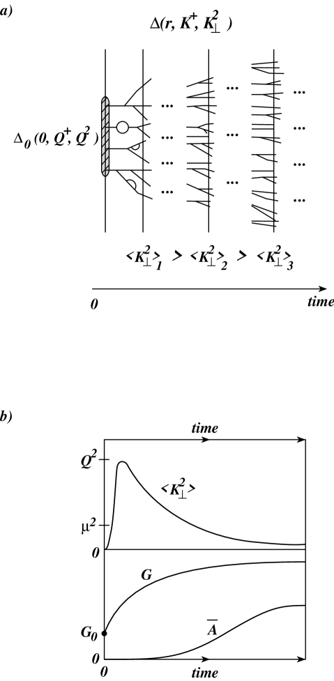
FIG. 1.: Non-equilibrium scenario of gluon beam along the lightcone: a) The initial multi-gluon state, prepared at time $t_{0}=0$ at the hard scale $Q$ with initial condition $\Delta_{0}(0,Q^{+},Q^{2})$, develops forward in time which is described by the evolution of the gluon propagator $\widehat{\Delta}(r,K^{+},K_{\perp}^{2})$ being a function of both space-time $r^{\mu}=(t,\vec{r})$ and momentum $K^{\mu}=(E,\vec{K})$. The gluons, propagating with large $K^{+}=E+K_{z}\gg K_{\perp}$ along the $z$-axis, are accompanied by real and virtual radiation which causes a diffusion in both transverse direction $r_{\perp}$ and transverse momentum $K_{\perp}$ as time goes on: The emission of gluons increases the multiplicity and decreases the average transverse momenta $\langle K_{\perp}^{2}\rangle$ at given lightcone time $r^{-}=t-z$ and position lightcone position $r^{+}=t+z$. b) Top: Qualitative picture of time evolution of the typical transverse momentum $\langle K_{\perp}^{2}\rangle$ of hard gluons, where the earliest emitted daughter gluons have the largest $K_{\perp}^{2}\,\lower 3.0pt\hbox{$\buildrel<\over{\sim}$}\,Q^{2}$ and later produced gluons have much smaller $K_{\perp}^{2}$. Eventually modes with $K_{\perp}^{2}<\mu^{2}$ will be populated significantly. Bottom: Corresponding time development of the number density ${\tt G}$ of hard gluons from initial value ${\tt G}_{0}$ and of the average soft field $\overline{A}$ that is induced by the population of gluons with $K_{\perp}^{2}<\mu^{2}$ , starting from zero initial value. Speculatively, one would expect a saturation at asymptotic times due to screening of further gluon emission by the presence of the soft mean field.

Given this heuristic picture, the near-at-hand rationale is therefore to subdivide the dynamical development of the gluon ensemble into a perturbative quantum evolution in the short-distance regime $Q^{2}\geq k_{\perp}^{2}\geq\mu^{2}$, and a non-perturbative, but classical, mean-field in the long-wavelength regime $k_{\perp}^{2}<\mu^{2}$. The corresponding degrees of freedom are referred to as hard gluons for $k_{\perp}\geq\mu$, whereas excitations with $k_{\perp}<\mu$ represent the soft mean field.

Because the hard gluons have small transverse extent $\lambda\sim 1/k_{\perp}\leq 0.2$ fm (for $\mu=1$GeV), they can be considered, locally in space-time, as incoherent self-interacting quanta, if the interparticle distance is significantly larger than $\lambda$. On the other hand, when the typical transverse momenta drop below $\mu$, the gluons begin to act coherently, and collectivity arises, because the motion taking place over a distance scale $1/\mu$ or larger, involves coherently a large number of hard particles, which gives rise to an average soft color field. The crucial point of this hard-soft separation is that the over long distances $\lambda>1/\mu$, the soft mean field represents the average gluon motion, but at short-distances $\lambda\leq 1/\mu$ the hard gluons may be described approximately as in free space. Certainly, such a rigid division of hard and soft physics in terms of a single parameter $\mu$, is at his point an arbitrary and idealizing definition. However, the arbitrariness can in principle be removed by considering the variation with respect to $\mu$, as in the usual renormalization-group framework. This interesting task is beyond the scope of this paper, and remains to be addressed in the future.

The non-quilibrium scenario of a lightcone beam of gluons along the lightcone has two major advantages over the opposite thermal equilibrium extreme, the isotropic quark-gluon plasma: First, it favors the 2-scale separation between hard and soft physics. Second, it allows to choose an axial-type gauge which eliminates to large extent the problems of non-linearities and of ghost degrees of freedom that are encountered in usual covariant gauges. The 2-scale separation arises naturally here, because Lorentz contraction and time dilation along the beam direction plus the limited transverse momenta, force the hard gluon fluctuations and self-interactions to be highly localized to short-distances, and separates their quantum motion from the low-momentum mean-field dynamics over comparably long distances. On the other hand, the choice of a non-covariant axial gauge, characterized by a directed four-vector $n$ along a fixed axis, is very suggestive, because the geometry and kinematics allows to choose $n$ paralell to the gluon momentum $k_{z}$, in which case perturbative QCD calculations formally reduce in many respects to the abelian QED counter parts. This is not possible for an isotropic thermal system, where all possible directions of gluon motion are equally probable. Given these premises, the quantum dynamics is dominated by the self-interactions of the hard gluons, which make them fluctuate localized around the lightcone, whereas the kinetic dynamics can well be desribed statistical-mechanically in terms of mutual interactions among them and in the presence of their generated soft mean field. As elaborated in Ref. [11], these notions are the keys to formulating a quantum-kinetic description, by combining standard techniques of parton evolution and renormalization group, with relativistic many-body transport theory.

The main result of this study within the outlined physics framework, is a set of three master equations, which couple the quantum evolution of short-distance fluctuations of the individual hard gluons, the space-time development of the gluon system as-a-whole, and the generation of the soft mean field:

  

(i) an evolution equation for the spectral density $\widehat{\rho}$ of each individual hard gluon, which determines the intrinsic gluon distribution of a hard gluon in accord with mass- and coupling-constant renormalization, and which dresses up the bare initial gluons to renormalized ‘quasi-particles’.

  

(ii) a transport equation for the space-time development of the whole ensemble of these renormalized gluons with respect to their propagation in the self-generated soft mean field, as well as due to their scatterings off each other, which determines the physical gluon phase-space density ${\tt G}$.

  

(iii) a Yang-Mills equation for the generation of the soft mean field $\overline{A}$, which is induced by the effective color current of the hard, renormalized gluons, where the current is obtained from the momentum-weighted gluon phase-space density.

Although this set of equations appears at first sight to be of impractical complexity, it allows in fact for a practical applicable calculation scheme, as will be demonstrated with an explicit sample calculation.

To arrive at the above master equations, three essential aspects of the problem have to be merged: first, the physics-dictated aspect of space-time, kinematics and geometry, second, the quantum field aspect of gluon excitations and self-interactions, and third, the statistical aspect of multi-particle interactions in the presence of the mean field. The non-trivial interconnection of these aspects require to work directly at the level of equations of motion, rather than on the level of Feynman diagrams, because the relative proportions and interactions of hard and soft quanta must can only be calculated self-consistently from the equations of motion.

The strategy for deriving the above three-some of master equations follows closely the previous work of Refs. [11]. The path-integral representation of the Yang-Mills action gives an infinite set of equations of motion for the non-equilibrium $n$-point Green functions, which is the well known analogue of the BBGKY hierarchy [14]. This hierarchy, which represents the exact theory, is truncated to a system of equations involving only the 1- and 2-point functions, by arguing that higher-order correlators $n\geq 3$ are comparably small. To achieve self-consistency of the truncated set of equations at the $n=2$ level, the $n\geq 3$ functions must be implicitely lumped into the 1- and 2-point functions. After separating hard and soft field modes, as alluded before, the 1-point function is identified with the soft average field $\overline{A}_{\mu}=\langle A_{\mu}(x)\rangle$ and the 2-point function is given by the hard gluon correlator $i\widehat{\Delta}_{\mu\nu}=\langle a_{\mu}(x)\,a_{\nu}(y)\rangle_{P}$, where $A_{\mu}$ and $a_{\mu}$ represent the soft and hard modes, repectively. The truncated set of equations of motion then involves the non-equilibrium version of the Dyson-Schwinger equation for $\widehat{\Delta}$ and the classical Yang-Mills equation for the soft mean-field $\overline{A}$. The two field-equations of motion for $\widehat{\Delta}$ and $\overline{A}$ can be cast into much simpler quantum-kinetic equations with the help of the Wigner-function technique and gradient expansion, and the assumption of 2-scale separation implying that the long-wavelength $\overline{A}$-field is slowly varying on the short-distance scale of the hard quantum fluctuations. The result is then the above set of master equations.

A powerful theoretical framework to derive from the exact field equations of motions the above approximate quantum kinetic equations, is the so-called Closed-Time-Path formalism (CTP). The CTP formalism is a general tool for treating initial value problems of irreversible multi-particle dynamics in quantum field theory. It therefore provides an appropriate language to describe the problem of non-equilibrium gluon dynamics within a well-established theoretical framework. Originally introduced by Schwinger [15] and Keldysh [16] the CTP formalism and its diverse applications is documented in great detail in the literature [17, 18, 19, 20, 21, 22, 23]. In particular, I refer to Ref. [11], where the CTP method is applied to high-energy QCD, and to Appendices B and C.

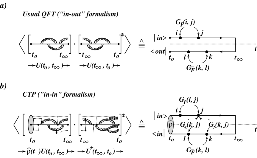
FIG. 2.: Difference between in-out formalism of usual quantum field theory (in free space or ‘vacuum’) and the in-in formalism of the CTP formulation (in the presence of surrounding particles or ‘medium’). a) The in-out amplitude describes by the evolution of an asymptotic $|in\rangle$ state at $t_{0}\rightarrow-\infty$ to an asymptotic $|out\rangle$ state at $t_{\infty}\rightarrow\infty$ by means of the time evolution operator $U(t_{0},t_{\infty})$. Because $U(t_{0},t_{\infty})=U^{\dagger}(t_{\infty},t_{0})$, forward and backward evolution are identical, and there is no correlation between the two time branches. Consequently, the Feynman propagator $G_{F}=G_{\overline{F}}^{\ast}$ contains the full dynamics of the 2-point correlations. b) The in-in amplitude starts at $t_{0}$ with a non-trivial initial multi-particle state described by the density matrix $\widehat{\rho}(t_{0})$ and evolves again by means of time evolution operator $U(t_{0},t_{\infty})$. Due to statistical interactions among the many evolving particles acting as a medium, in this case $\widehat{\rho}(t_{0})U(t_{0},t_{\infty})\neq U^{\dagger}(t_{\infty},t_{0})$. Consequently, the statistical correlation between the two time branches have the effect that $G_{F}\neq G_{\overline{F}}^{\ast}$, and moreover require the introduction of additional correlation functions $G_{>}$ and $G_{<}$ to account for the cross-talk between upper and lower time branches.

The fundamental starting point of non-equilibrium field theory in the CTP formalism is to write down the in-in amplitude $Z_{P}$ for the evolution of the initial quantum state $|in\rangle$ forward in time into the remote future. As reviewed in Appendix B, this generalizes the usual quantum field theory approach based on the vacuum-vacuum transition amplitude, or in-out amplitude, to account for the a-priori-presence of medium particles described by the density matrix $\hat{\rho}(t_{0})$ and to evolve this non-trivial initial state in the presence of the medium from $t_{0}$ to $t_{\infty}$ in the future, The in-in amplitude $Z_{P}$ is graphically depicted in Fig. 2, and formally it is given by $Z_{P}[{\cal J},\hat{\rho}]=\langle\;in\;|\;in\;\rangle_{{\cal J},\hat{\rho}}$, where ${\cal J}=({\cal J}^{+},{\cal J}^{-})$ is an external source with components on the upper $+$ and lower $-$ time branch, and $\hat{\rho}(t_{0})$ denotes the the initial state density matrix. From the path-integral representation of $Z_{P}$ one obtains then the non-equilibrium Green functions. The convenient feature of this Green function formalism on the closed-time path $P$ is that it is formally analogous to standard quantum field theory, based on the vacuum-vacuum, or in-out amplitude $Z[{\cal J}]=\langle\;out\;|\;in\;\rangle_{{\cal J}}=\langle 0|0\rangle_{{\cal J}}$, except for the fact that in the CTP formalism, the fields have contributions from both time branches. For details I refer to Appendix B, where the basics of the CTP formalism are summarized, in particular, how to obtain the path-integral for $Z_{P}$ that generates the Green functions on the closed-time-path $P$.

The interpretation of this formal apparatus for the evolution along the closed-time path $P$ is rather simple: If the initial state is the vacuum itself, that is, the absence of a medium generated by other particles, then the density matrix $\hat{\rho}$ is diagonal and one has $|in\rangle\rightarrow|0\rangle$. In this case the evolution along the $+$ branch is identical to the anti-time ordered evolution along the $-$ branch (modulo an irrelevant phase), and space-time points on different branches cannot cross-talk. In the presence of a medium however, the density matrix contains off-diagonal elements, and there are statistical correlations between the quantum system and the medium particles (e.g. scatterings) that lead to correlations between space-time points on the $+$ branch with space-time points on the $-$ branch. Hence, when addressing the evolution of a multi-particle system, both the deterministic self-interaction of the quanta, i.e. the time- (anti-time-) ordered evolution along the $+$ ($-$) branch, and the statistical mutual interaction with each other, i.e. the non-time-ordered cross-talk between $+$ and $-$ branch, must be included in a self-constistent manner. The CTP method achieves this through the time integtation along the contour $P$. Although for physical observables the time values are on the $+$ branch, both $+$ and $-$ branches will come into play at intermediate steps in a self-consistent calculation.

The outline of the paper is as follows: In Section 2 the field equations of motion for the hard gluon propagator and the soft mean field are derived from the path-integral representation of the in-in amplitude $Z_{P}$ for non-covariant gauges. After separating hard and soft degrees of freedom, two key approximations are made, that allow to cast the infinite hierarchy of exact equations of motion in terms of a truncated system of only two approximate equations, namely a Dyson-Schwinger equation for the hard gluon propagator, and a Yang-Mills equation for the soft field. In Section 3 the transition to a quantum kinetic description is worked out. This requires one further key approximation in conjunction with a clear definition of quantum and kinetic space-time regimes, such that the aforementioned 2-scale separation is guaranteed. This also defines the limits for the applicability of the quantum kinetic approximation. Provided that the separability condition is satisfied, one finally arrives at the set of master equations discussed above, for which a systematic calculation scheme is proposed. In Section 4 an explicit calculation to solve the master equations is presented for the physics scenario depicted in Fig. 1. I consider the evolution of an initial incoherent ensemble of bare gluons moving colinearly along the lightcone as it proceeds in its momentum- and space-time development and generates its soft mean field. To avoid overkill of too many technical details, each Section is accompanied by Appendices. Appendix A defines the notation and conventions used throughout the paper. Appendix B reviews the basics of the CTP formalism. Appendix C discusses the application of the CTP method to QCD for non-covariant gauges. Appendix D shows the advantagous absence of ghosts in non-covariant gauges. Appendix E gives details on how to obtain from the in-in amplitude ${\cal Z}_{P}$ an approximate effective action functional from which the of motion for the hard gluon propagator and the soft field are derived. Appendix F summarizes some basic analycity properties of the free-field propagators in the CTP formalism and discusses their relation to the gluon phase-space density.

Finally some remarks on most closely related work in the literature (for an extended discussion, see introduction of Ref. [11]):

Blaizot and Iancu [10] have in a series of papers developed a kinetic theory for ‘hot QCD’, i.e. the case of a high-temperature quark-gluon plasma. One of the key elements of their approach is the formulation of well-defined and consistent approximation scheme. I adopted many features of this approach to the present, rather different physics context. New is here the inclusion of the aspect of quantum evolution and renormalization.

McLerran, Venugopalan, et al. [24], as well as Makhlin [25], have developed different approaches to calculate the quantum evolution of parton systems with lightcone dominance, i.e. in a beam-type scenario as considered in the present work. The McLerran-Venugopalan model also gives a predictive estimate for the feedback effect of the coherent mean field on the hard gluon evolution that generates this field. In several respects I follow a similar route. New in the present work is that it embodies in addition the aspect of space-time development of the evolution.

Boyanovski et al. have intensly studied the non-equilibrium evolution in scalar field theory, using extensively the techniques of the CTP formalism in conjunction with a large-$N$ expansion. Although the focus on this paper is rather different, many of the concepts and results in their papers concerning the first-principle time evolution of quantum system with associated particle production, dissipation, mean-field dynamics, etc., may serve as a scalar toy model for QCD.

II INTERPLAY OF ‘HARD’ AND ‘SOFT’ GLUON DYNAMICS

A The in-in amplitude for QCD in non-covariant gauges and the concept of approximation

The in-in amplitude $Z_{P}$ introduced in Sec. 1 admits a path-integral representation which is the generating functional for the non-equilibrium Green functions defined on closed-time-path $P$, as discussed in Appendices B and C:

$$Z_{P}[{\cal K}]\;=\;\int\,{\cal D}{\cal A}\;\exp\left\{i\left(\frac{}{}I\left[{\cal A},{\cal K}\right]\right)\right\}\;,$$ (1)

where ${\cal A}_{\mu}^{a}=({\cal A}^{a\;+}_{\mu},{\cal A}^{a\;-}_{\mu})$ has two components, living on the upper ($+$) and lower ($-$) time branches of Fig. 2, with ${\cal D}{\cal A}=\prod_{\mu,a}{\cal D}{\cal A}^{a\;+}_{\mu}{\cal D}{\cal A}^{a\;-}_{\mu}$, and ${\cal K}$ represents the presence of external sources. I consider here the class of non-covariant gauges defined by [27, 28],

$$\langle\;n^{\mu}\,{\cal A}_{\mu}^{a}(x)\;\rangle\;=\;0\;,$$ (2)

where $n^{\mu}$ is a constant 4-vector, being either space-like ($n^{2}<0$), time-like ($n^{2}>0$), or light-like ($n^{2}=0$). The particular choice of the vector $n^{\mu}$ is usually dictated by the physics or computational convenience, and distinguishes axial gauge ($n^{2}<0$), temporal gauge ($n^{2}>0$), and lightcone gauge ($n^{2}=0$). Referring to Appendix D, the great advantage of these gauges is that the Fadeev-Popov ghosts decouple, so that in practical calculations the ghost degrees of freedom can be ignored, just as in abelian gauge theories.

Then the action $I$ in the exponential of (1) is given by (c.f. Appendix C),

$$I\left[{\cal A},{\cal K}\right]\;\equiv\;I_{YM}\left[{\cal A}\right]\;+\;I_{GF}\left[n\cdot{\cal A}\right]\;+\;{\cal K}[{\cal A}]\;,$$ (3)

containing the Yang-Mills action $I_{YM}$, the gauge fixing term $I_{GF}$, and the initial state source term ${\cal K}$, containing multi-point correlations concentrated at $t=t_{0}$:

$$I_{YM}\left[{\cal A}\right] = -\frac{1}{4}\int_{P}d^{4}x\,{\cal F}_{\mu\nu}^{a}(x){\cal F}^{\mu\nu,\,a}(x)\;,\;\;\;\;\;\;\;\;\;\;\;\;\;\;\;I_{GF}\left[n\cdot{\cal A}\right]\;=\;-\frac{1}{2\alpha}\int_{P}d^{4}x\,\left[n\cdot{\cal A}^{a}(x)\right]^{2}\;,$$ (4)

$${\cal K}[{\cal A}] = {\cal K}^{(0)}\;+\;\int_{P}d^{4}x\;{\cal K}^{(1)\;a}_{\;\;\;\,\mu}(x)\;{\cal A}^{\mu,\,a}(x)\;+\;\frac{1}{2}\int_{P}d^{4}xd^{4}y\;{\cal K}^{(2)\;ab}_{\;\;\;\,\mu\nu}(x,y)\;{\cal A}^{\mu,\,a}(x)\,{\cal A}^{\nu,\,b}(y)\;\;+\;\;\ldots\;.$$ (5)

The exact knowledge of the in-in amplitude $Z_{P}$ from (1), would require to the calculation of all Green functions up to infinite order, and would correspond to the full solution of QCD in non-equilibrium media. Rather than that, the realistic goal is to formulate a practical calculation scheme for the kinetic evolution of a multi-guon system. In order to make progress, one needs to make reasonable approximations that are consistent with the specific physical problem under study, and truncate the infinite hierarchy of Green functions.

In this Section a closed set of approximate equations is derived that are in principle solvable, given a suitable physics scenario. The basic idea is to describe an evolving gluon system in terms of two distinct components, namely, hard, short-range quantum fluctuations and soft, long-wavelength collective excitations, which I assume to be separable by a characteristic space-time distance. It is clear that the relative proportions and interactions of hard and soft degrees of freedom must be calculated self-consistently from the equations of motion.

Starting from the in-in amplitude (1), the strategy of procedure is the following:

  1.

The exact expression of the in-in amplitude $Z_{P}\equiv\exp(iW_{P})$ is rewritten in terms of soft and hard field modes by splitting the gauge field ${\cal A}_{\mu}=A_{\mu}+a_{\mu}$. Therefrom one obtains an infnite set of coupled equations for the Green functions. In order to reduce this to a finite system, I make

• approximation 1: The functional $W_{P}=-i\ln Z_{P}$ is expressed in terms of connected 1- and 2-point functions ${\cal G}^{(1)}$, ${\cal G}^{(2)}$ alone by eliminating ${\cal G}^{(n)}$ for $n\geq 3$ as dynamical variables. Then the expectation values of ${\cal G}^{(1)}$ and ${\cal G}^{(2)}$ describe the induced soft mean field $\overline{A}_{\mu}$ and the hard (soft) correlation functions $\widehat{\Delta}_{\mu\nu}$ ($\widehat{D}_{\mu\nu}$).

  2.

From the truncated functional $W_{P}$ the corresponding effective action $\Gamma_{P}$ is obtained, which generates the desired self-consistent equations of motion for $\overline{A}_{\mu}$, $\widehat{\Delta}_{\mu\nu}$ and $\widehat{D}_{\mu\nu}$. Here I make

• approximation 2: It is assumed that the soft field dynamics can be treated classically by the non-propagating average field $\overline{A}_{\mu}$, and that the long-range propagation of soft modes, described by $\widehat{D}_{\mu\nu}$ may be ignored at this level, i.e. $\widehat{D}_{\mu\nu}\ll\overline{A}_{\mu}\overline{A}_{\nu}$. This assumption is motivated by the widely studied [24, 13] observation that a classical treatment of the long-distance dynamics of bosonic quantum fields at high density, obeying the classical field equations, should provide a good approximation, if the soft modes are sufficiently occupied.

The original infinite equation system can then be reduced to a Yang-Mills equation for the classical, soft field $\overline{A}_{\mu}$, as it is induced by the current of hard quanta, and a Dyson-Schwinger equation for the hard propagator $\widehat{\Delta}_{\mu\nu}$ subject to the presence of the soft mean field and to quantum fluctuations. These field equations of motion are still of very intractable non-linear character. They are further simplified to quantum-kinetic equations in Sec. III.

B Separating soft and hard dynamics

The first step in the strategy is the separation of soft and hard physics in the path-integral formalism with Green functions of both the soft and hard quanta in the presence of the soft classical field that is induced by and feeding back to the quantum dynamics. A frequently used method for separate treatment of quantum and classical dynamics in field theory is the so-called ‘background field method’ [29] which has been studied, e.g., in the context of dynamical symmetry breaking, vacuum structure, confinement and gravity, or for hot plasmas in finite temperature QCD. Within the background field method, one would split up the gauge field appearing in the classical action into an external classical background field and a quantum field which remains the sole dynamical variable in the path integral. I will however not follow this path, and rather prefer to treat soft and hard physics on equal footing, that is, to separate the gauge field into a soft classical field plus its soft quantum excitations, and a hard quantum field. Then both soft and hard fields can quantized and remain as dynamical variables a priori.

The gauge field ${\cal A}_{\mu}$ appearing in the classical action $I_{YM}\left[{\cal A}\right]$ is split up into a soft ( long-range) part $A_{\mu}$, and a hard (short-range) quantum field $a_{\mu}$:

$${\cal A}_{\mu}^{a}(x)\;=\;\int\frac{d^{4}k}{(2\pi)^{4}}\,e^{+ik\cdot x}{\cal A}_{\mu}^{a}(k)\;\,\theta(\mu^{2}-k_{\perp}^{2})\;\,+\;\,\int\frac{d^{4}k}{(2\pi)^{4}}\,e^{+ik\cdot x}{\cal A}_{\mu}^{a}(k)\,\;\theta(k_{\perp}^{2}-\mu^{2})\;\;\equiv\;\;A_{\mu}^{a}(x)\;+\;a_{\mu}^{a}(x)\;.$$ (6)

This is the formal definition of the terms ‘soft’ and ‘hard’, as used in this paper. The soft and hard physics are separated by the momentum scale $\mu$ which is at this point arbitrary. However, this arbitrariness can in principle be overcome by considering $\mu(x)$ as a dynamical variable depending on the space-time point $x$, rather than a fixed parameter, and determining it self-consistently from the local stability condition $d{\cal A}_{\nu}(x)/d\mu^{2}(x)=0$. From (6) it is obvious, that the corresponding scale in space-time, $\lambda\equiv 1/\mu$, divides soft and hard regimes in terms of the transverse wavelength of field modes, so that one may associate the soft field $A_{\mu}$ being responsible for long range color collective effects, and the hard field $a_{\mu}$ embodying the short-range quantum dynamics. Consequently, the field strength tensor receives a soft part, a hard part, and a mixed contribution,

$${\cal F}_{\mu\nu}^{a}(x)\;\equiv\;\left(\frac{}{}F_{\mu\nu}^{a}[A]\;+\;f_{\mu\nu}^{a}[a]\;+\;\phi_{\mu\nu}^{a}[A,a]\right)(x)\;.$$ (7)

When quantizing this decomposed theory by writing down the appropriate in-in-amplitude $Z_{P}$, one must be consistent with the gauge field decomposition (6) into soft and hard components and with the classical character of the former. Substituting the soft-hard mode decomposition (6) into (1), the functional integral of the in-in amplitude (C17) becomes:

$$Z_{P}[{\cal K}]\;=\;\int\,{\cal D}A\,{\cal D}a\;\exp\left\{i\left(\frac{}{}I\left[A\right]\;+\;I\left[a\right]\;+\;I\left[A,a\right]\right)\right\}\;,$$ (8)

with the soft, hard, and mixed contribution, respectively,

$$I\left[A\right] = \int d^{4}x\left(\frac{}{}-\frac{1}{4}F_{\mu\nu}^{a}F^{\mu\nu,\;a}-\frac{1}{2\alpha}\,(n\cdot A^{a})^{2}\right)$$ (10)

$$\;\;\;\;\;\;\;\;\;\;\;\;\;\;\;\;\;\;\;\;\;\;\;\;\;\;\;\;\;\;\;\;\;\;\;\;\;\;\;\;\;\;+\;\int d^{4}x\;{\cal K}_{\;\;\;\mu}^{(1)\;a}A^{\mu,\;a}\;+\;\int d^{4}xd^{4}y\;A^{\mu,\;a}\,{\cal K}_{\;\;\;\mu\nu}^{(2)\;ab}\,A^{\nu,\;b}\;\;+\;\;\ldots\;,$$

$$I\left[a\right] = \int d^{4}x\left(\frac{}{}-\frac{1}{4}f_{\mu\nu}^{a}f^{\mu\nu,\;a}-\frac{1}{2\alpha}\,(n\cdot a^{a})^{2}\right)$$ (12)

$$\;\;\;\;\;\;\;\;\;\;\;\;\;\;\;\;\;\;\;\;\;\;\;\;\;\;\;\;\;\;\;\;\;\;\;\;\;\;\;\;\;\;+\;\int d^{4}x\;{\cal K}_{\;\;\;\mu}^{(1)\;a}a^{\mu,\;a}\;+\;\int d^{4}xd^{4}y\;a^{\mu,\;a}\,{\cal K}_{\;\;\;\mu\nu}^{(2)\;ab}\,a^{\nu,\;b}\;\;+\;\;\ldots\;,$$

$$I\left[A,a\right] = \int d^{4}x\left(\frac{}{}-\frac{1}{4}\phi_{\mu\nu}^{a}\phi^{\mu\nu,\;a}-\frac{1}{2}\left\{\phi_{\mu\nu}^{a}F^{\mu\nu,\;a}\;+\;\phi_{\mu\nu}^{a}f^{\mu\nu,\;a}\;+\;F_{\mu\nu}^{a}f^{\mu\nu,\;a}\right\}\right)$$ (13)

$$= \int d^{4}x\left\{\frac{}{}-gf^{abc}\left[\frac{}{}\;(\partial_{\mu}^{x}A_{\nu}^{a})\;\left(a^{\mu,\;b}a^{\nu,\;c}+A^{\mu,\;b}a^{\nu,\;c}+a^{\mu,\;b}A^{\nu,\;c}\right)\right.\right.$$ (16)

$$\left.\frac{}{}\;\;\;\;\;\;\;\;\;\;\;\;\;\;\;\;\;\;\;\;\;\;\;\;\;\;\;\;\;\;\;\;\;\;\;\;\;+\;(\partial_{\mu}^{x}a_{\nu}^{a})\;\left(A^{\mu,\;b}A^{\nu,\;c}+a^{\mu,\;b}A^{\nu,\;c}+A^{\mu,\;b}a^{\nu,\;c}\right)\right]$$

$$\left.\;\;\;\;\;\;\;\;\;\;\;\;-\;g^{2}f^{ace}f^{bde}\left[\frac{}{}2\,A_{\mu}^{a}A_{\nu}^{b}a^{\mu,\;c}a^{\nu,\;d}\;+\;A_{\mu}^{a}A_{\nu}^{b}A^{\mu,\;c}a^{\nu,\;d}\;+\;a_{\mu}^{a}a_{\nu}^{b}a^{\mu,\;c}A^{\nu,\;d}\right]\;\right\}\;.$$

Note that in (12) and (16) terms involving 2-products $\propto a_{\mu}\,A_{\nu}$ do not contribute to $Z_{P}$, because their expectation value vanishes due to the soft-hard separation (6) which defines $a_{\mu}$ and $A_{\nu}$ as complimentary.

At this point I make approximation 1 from above. It is assumed that initial state can be represented as an ensemble of incoherent hard gluons, each of which has very small spatial extent $\Delta r_{\perp}\ll\lambda=1/\mu$, corresponding to transverse momenta $k_{\perp}^{2}\gg\mu^{2}$. By definition of $\mu$, the short-range character of these quantum fluctuations implies that the expectation value $\langle a_{\mu}\rangle$ vanishes at all times. However, the long-range correlations of the eventually populated soft modes with small momenta $k_{\perp}^{2}\leq\mu^{2}$ may lead to a collective mean field with non-vanishing $\langle A_{\mu}\rangle$. Accordingly, I impose the following condition on the expectation values of the fields:

$$\langle\;A_{\mu}^{a}(x)\;\rangle\;\left\{\begin{array}[]{ll}\;=\;0\;\;\;\mbox{for}\;t\,\leq\,t_{0}\\ \;\geq\;0\;\;\;\mbox{for}\;t\,>\,t_{0}\end{array}\right.\;\;\;\;\;\;\;\;\;\;\;\;\;\;\;\;\;\;\;\;\langle\;a_{\mu}^{a}(x)\;\rangle\;\stackrel{{\scriptstyle!}}{{=}}\;0\;\;\;\mbox{for all}\;t\;.$$ (17)

Now I make approximation 2, that is, the quantum fluctuations of the soft field are ignored, assuming any multi-point correlations of soft fields to be small,

$$\langle\;A_{\mu_{1}}^{a_{1}}(x_{1})\;\ldots A_{\mu_{n}}^{a_{n}}(x_{n})\;\rangle\ll\;\langle\;A_{\mu_{1}}^{a_{1}}(x_{1})\;\rangle\;\ldots\;\langle\;A_{\mu_{1}}^{a_{n}}(x_{n})\;\rangle\;\;\;\;\;\;\mbox{for all $n\geq 2$}\;,$$ (18)

i.e. take $A_{\mu}$ as a non-propagating and non-fluctuating, classical field. In particular,

$$iD_{\mu\nu}^{ab}(x,y)\;\equiv\;\langle\;A_{\mu}^{a}(x)A_{\nu}^{b}(y)\;\rangle\ll\;\langle\;A_{\mu}^{a}(x)\;\rangle\;\langle\;A_{\nu}^{b}(y)\;\rangle\;,$$ (19)

so that the limit ”$D_{\mu\nu}\rightarrow 0$” can be considered.

As explained in more detail in Appendix E, the generating functional for the connected Green functions,

$$W_{P}\left[{\cal K}\right]\;\;=\;\;-i\,\ln\,Z_{P}\left[{\cal K}\right]\;,$$ (20)

which generates the infinite set of connected $n$-point Green functions ${\cal G}^{(n)}$ via

$$(-i)\,{\cal G}_{\;\;\;\;\mu_{1}\ldots\mu_{n}}^{(n)\;a_{1}\ldots a_{n}}(x_{1},\ldots,x_{n})\;\equiv\;\left.\frac{\delta}{i\,\delta{\cal K}^{(n)}}W_{P}[{\cal K}]\right|_{{\cal K}=0}\;\;=\;\;\langle\;a_{\mu_{1}}^{a_{1}}(x_{1})\ldots a_{\mu_{k}}^{a_{k}}(x_{k})\,A_{\mu_{k+1}}^{a_{k+1}}(x_{k+1})\ldots A_{\mu_{n}}^{a_{n}}(x_{n})\;\rangle_{P}^{(c)}\;,$$ (21)

is truncated at level $n\geq 3$ on the basis of approximation (17) and (19). As a result, $W_{P}$ becomes a functional of the 1-point function (soft mean field $\overline{A}$) and the 2-point function (hard propagator $\widehat{\Delta}$) only:

$${\cal G}_{\;\;\;\;\mu}^{(1)\;a}(x)\;=\;\langle\;A_{\mu}^{a}(x)\;\rangle_{P}^{(c)}\;\;\equiv\;\;\overline{A}_{\mu}^{a}(x)\;\;\;\;\;\;\;\;\;{\cal G}_{\;\;\;\;\mu\nu}^{(2)\;ab}(x,y)\;=\;\langle\;a_{\mu}^{a}(x)a_{\nu}^{b}(y)\;\rangle_{P}^{(c)}\;\;\equiv\;\;i\widehat{\Delta}_{\mu\nu}^{ab}(x,y)\;.$$ (22)

These relations define the soft, classical mean field $\overline{A}$, and the hard quantum propagator $\widehat{\Delta}$ in terms of expectation values of soft and hard field operators $A_{\mu}$ and $a_{\mu}$, respectively. One now readily one obtains the effective action $\Gamma_{P}$ (or proper vertex functional) via Legendre transformation (c.f. Appendix E):

$$\Gamma_{P}\left[{\cal G}\right]\;\;\approx\;\;\Gamma_{P}\left[\overline{A},\widehat{\Delta}\right]\;\;=\;\;W_{P}\left[{\cal K}^{(1)},{\cal K}^{(2)}\right]\;-\;{\cal K}^{(1)}\circ\overline{A}\;-\;\frac{1}{2}\;{\cal K}^{(2)}\circ\left(\,i\widehat{\Delta}\;+\;\overline{A}\;\overline{A}\right)\;,$$ (23)

which is a functional of only the soft field $\overline{A}$ and the hard propagator $\widehat{\Delta}$ as independent dynamical degrees of freedom.

The equations of motion for the mean field $\overline{A}$ and for the hard propagator $\widehat{\Delta}$ in the presence of sources, follow now by differentiaition of (23) with respect to $\overline{A}$ and $\widehat{\Delta}$ (c.f. Appendix E):

$$\frac{\delta\Gamma_{P}}{\delta\overline{A}_{\mu}^{a}(x)} = -{\cal K}^{(1)\;\mu,a}(x)\;-\;\int_{P}d^{4}y\,K^{(2)\;\mu\nu,ab}(x,y)\;\overline{A}^{\nu,\,b}(y)\;,$$ (24)

$$\frac{\delta\Gamma_{P}}{\delta\widehat{\Delta}_{\mu\nu}^{ab}(x,y)} = \frac{1}{2i}\;{\cal K}^{(2)\;\mu\nu,ab}(x,y)\;.$$ (25)

The self-consistent equations of motion of the dynamically evolving system are then obtained from (24) and (25) by (i) imposing initial conditions in terms of the ${\cal K}$ kernels at $t=t_{0}$, and (ii) by obtaining an explicit formula for $\Gamma_{P}$ in terms of $\overline{A}_{\mu}$ and $\widehat{\Delta}_{\mu\nu}$. Concerning the initial conditions, I restrict to non-equilibrium initial states of Gaussian form (i.e. quadratic in the hard modes) and do not consider possible linear force terms. That is, I set

$$\left.{\cal K}^{(1)}(x)\right|_{x^{0}=t_{0}}\;=\;0\;,\;\;\;\;\;\;\left.{\cal K}^{(2)}(x,y)\right|_{x^{0}=y^{0}=t_{0}}\;\geq\;0\;.$$ (26)

To obtain an explicit expression for $\Gamma_{P}$, the formal loop expansion of (23) results in the well known Cornwall-Jackiw-Tomboulis formula [30]:

$$\Gamma_{P}\left[\overline{A},\widehat{\Delta}\right]\;=\;\;\overline{I}_{eff}[\overline{A},a]\;-\;\frac{i}{2}\,\mbox{Sp}\left[\;\ln(\Delta_{0}^{-1}\widehat{\Delta})\,-\,\overline{\Delta}_{0}^{\;-1}\widehat{\Delta}\,+\,1\;\right]\;\;+\;\;\Gamma_{P}^{(2)}\left[\overline{A},\widehat{\Delta}\right]\;,$$ (27)

where $\mbox{Sp}[AB\ldots]\equiv\mbox{Tr}\int_{P}d^{4}x_{1}d^{4}x_{2}\ldots A(x_{1})B(x_{2})\ldots$ stands for both the trace over color and Lorentz indices, as well as the integration over all space-time positions, hence giving the expectation value $\langle AB\ldots\rangle_{P}$ as defined in Appendix C. The physical interpretation of the various terms in this expression for $\Gamma_{P}$ is the following [11]:

  (i)

The first term is of order $\hbar^{0}$ and is given by the classical action (10)-(12) at $A=\overline{A}$ and switched-off sources ${\cal K}$:

$$\overline{I}_{eff}[\overline{A},a]\;\equiv\;\left[\frac{}{}I\left[A\right]\;+\;I\left[a\right]\;+\;I\left[A,a\right]\right]_{A=\overline{A},\,{\cal K}=0}\;.$$ (28)

Notice that in the limit $a=0$, this reduces to the classical action for the soft mean field, $\overline{I}_{eff}[\overline{A},0]=I_{YM}[\overline{A}]+I_{GF}[n\cdot\overline{A}]$.

  (ii)

The second term in (27) is of order $\hbar^{1}$ and contains the the contributions of the coupling between the soft mean field $\overline{A}$ and the hard quantum propagator $\widehat{\Delta}$. The free propagator (see Fig. 3a) is given by $[\delta^{2}\overline{I}_{eff}[\overline{A},a]/\delta a(x)\delta a(y)]_{A=0;\,a=0}$ with $\overline{A}$ switched off, which yields

$$(\Delta_{0}^{-1})_{\mu\nu}^{ab}(x,y)\;\;=\;\;-\;\delta_{ab}\,\delta_{P}^{4}(x,y)\;\;d_{\mu\nu}(\partial_{x})\;\;\partial_{x}^{2}\;,$$ (29)

where it is understood that the space-time arguments $x$ and $y$ in $\Delta_{0}$ satisfy $(x-y)_{\perp}^{2}<1/\mu^{2}$, and

$$d_{\mu\nu}(\partial_{x})\;\equiv\;g^{\mu\nu}\;-\;\frac{n^{\mu}\partial_{x}^{\nu}+n^{\nu}\partial_{x}^{\mu}}{n\cdot\partial_{x}}\;+\;\left(n^{2}+\alpha^{-1}\partial_{x}^{2}\right)\,\frac{\partial^{\mu}_{x}\partial^{\nu}_{x}}{(n\cdot\partial_{x})^{2}}\;,$$ (30)

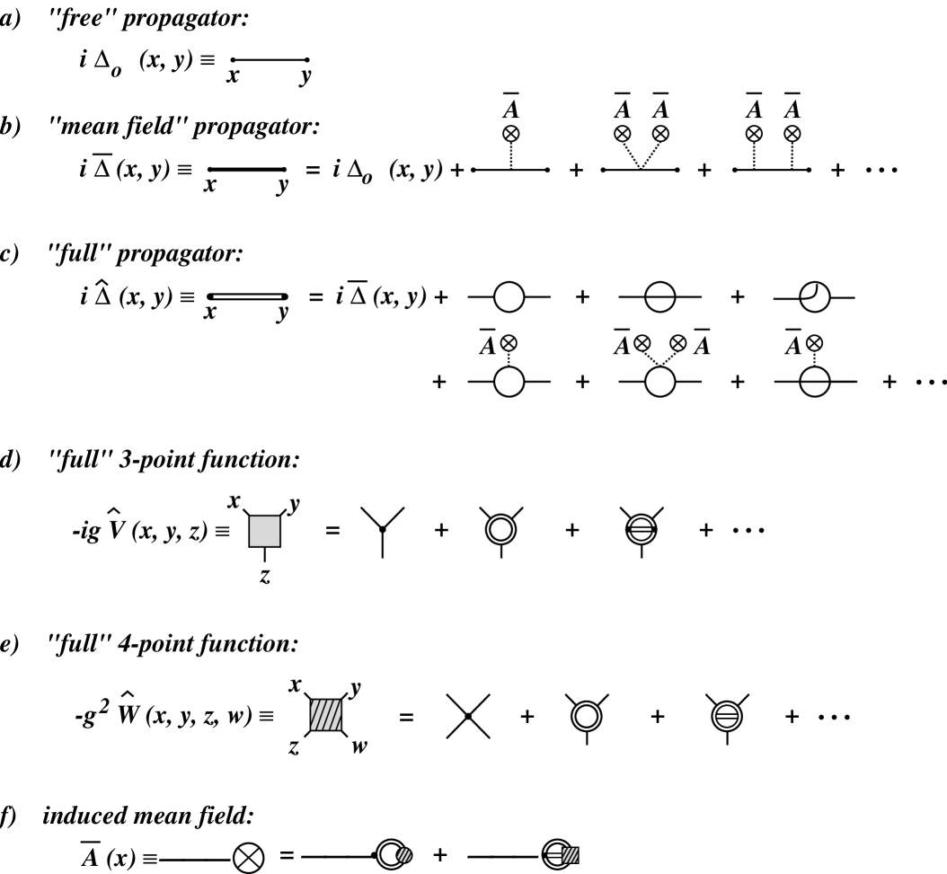
FIG. 3.: Diagrammatics of the various terms used for the $n$-point functions appearing in the text. The 2-point function ${\cal G}^{(2)}=i\Delta$ is the hard gluon propagator with the free-field propagator $\Delta_{0}$ (no interactions), the mean-field propagator $\overline{\Delta}$ (including the interactions with the classical soft field $\overline{A}$), and the full propagator $\widehat{\Delta}$ (including both mean-field and quantum (loop) interactions). Similarly, the connected 3-point function ${\cal G}^{(3)}=-ig\widehat{V}$ and the 4-point function ${\cal G}^{(4)}=-g^{2}\widehat{W}$ contain soft mean-field plus hard quantum contributions with internal full propagator $\widehat{\Delta}$. Finally, the 1-point function is the soft mean field $\overline{A}$ that is generated by the hard gluons through the coupling to the full 3-point and 4-point functions $\widehat{V}$ and $\widehat{W}$.

Even in the absence of quantum fluctuations, these contributions amount to a modification of the free propagator, such that the free propagator $\Delta_{0}$ becomes an effective propagator $\overline{\Delta}$ in the mean field, dressed up by the presence of $\overline{A}$. This mean field propagator (see Fig. 3b), denoted by $\overline{\Delta}$, is obtained from $[\delta^{2}\overline{I}_{eff}[\overline{A},a]/\delta a(x)\delta a(y)]_{A=\overline{A};\,a=0}$ with finite $\overline{A}\neq 0$, which results in

$$(\overline{\Delta}^{\;-1})_{\mu\nu}^{ab}(x,y)\;\;=\;\;(\Delta_{0}^{-1})_{\mu\nu}^{ab}(x,y)\;\,-\;\,\overline{\Pi}_{\mu\nu}^{ab}(x,y)\;,$$ (31)

where $\overline{\Pi}$ denotes the self-energy contribution associated with the presence of the mean-field $\overline{A}\neq 0$. Its explicit expression is given below in (59). In other words, the effect of the mean field is to shift the pole in the free propagator $\Delta_{0}$ of (29) by a dynamically induced ‘mass’ term $\propto\overline{\Pi}$, which can produce screening and damping effects. Note that $\Delta_{0}^{-1}=\overline{\Delta}^{\;-1}|_{\overline{A}=0}$. It is important to realize that this mean field effect is still on the classical tree-level, and does not involve quantum fluctuations associated with radiative self-interactions among the hard gluons.

  (iii)

The last term $\Gamma_{P}^{(2)}$ in (27) represents the sum of all two-particle irreducible graphs of order $\hbar^{2},\hbar^{3},\ldots$ [30], with the full propagator $\widehat{\Delta}$, dressed by both the soft mean field and the quantum self-interactions (see Fig. 3c),

$$\widehat{\Delta}_{\mu\nu}^{ab}(x,y)\;\equiv\;\widehat{\Delta}_{[\overline{0}]\;\mu\nu}^{ab}(x,y)\;+\;\delta\widehat{\Delta}_{[\overline{A}]\;\mu\nu}^{ab}(x,y)\;,$$ (32)

where the dependence of the full propagator on the soft mean field $\overline{A}$ is indicated by an explicit subscript, and

$$\widehat{\Delta}_{[\overline{0}]\;\mu\nu}^{ab}\;=\;\left.\widehat{\Delta}_{[\overline{A}]\;\mu\nu}^{ab}\right|_{\overline{A}=0}\;\;\;\;\;\;\;\;\;\;\;\left.\delta\widehat{\Delta}_{[\overline{A}]\;\mu\nu}^{ab}\right|_{\overline{A}=0}\;=\;0\;.$$ (33)

Note that $\widehat{\Delta}_{[\overline{0}]}\neq\Delta_{0}$, that is, $\widehat{\Delta}_{[\overline{0}]}$ denotes the full propagator for $\overline{A}=0$, whereas $\Delta_{0}$ is the free propagator (29). The real (dispersive) part of $\Gamma_{P}^{(2)}$ contains the virtual loop corrections associated with the gluon self-interactions, whereas the imaginary (dissipative) part contains the emission, absorption, and scattering processes of hard gluons. In other words, $\Gamma_{P}^{(2)}$ embodies all the interesting quantum dynamics that is connected with renormalization group, entropy generation, dissipation, etc.. The explicit form of $\Gamma_{P}^{(2)}$ is diagramatically shown in Fig. 4, with the vertices and lines defined by Fig. 3. Suppressing color and Lorentz indices and employing a condensed notation, e.g., $\widehat{\Delta}(x_{1},x_{2})\equiv\widehat{\Delta}_{\mu\nu}^{ab}(x_{1},x_{2})$, the corresponding formula is,

$$\Gamma_{P}^{(2)}\left[\overline{A},\widehat{\Delta}\right]\;=\;\Gamma_{(1)}\;+\;\Gamma_{(2)}\;+\;\Gamma_{(3)}\;+\;\Gamma_{(4)}\;,$$ (34)

with the following contributions,

$$\Gamma_{(1)} = \;\frac{1}{8}\,g^{2}\;\;\int_{P}d^{4}xd^{4}y\int_{P}d^{4}x_{1}d^{4}y_{1}W_{0}(x,y,x_{1},y_{1})\;\widehat{\Delta}(y_{1},x_{1})\;\widehat{\Delta}(y,x)$$ (35)

$$\Gamma_{(2)} = \;\frac{i}{12}\,g^{2}\;\;\int_{P}d^{4}xd^{4}y\int_{P}\prod_{i=1}^{2}d^{4}x_{i}d^{4}y_{i}\;\;V_{0}(x,x_{1},x_{2})\;\;\widehat{\Delta}(x_{1},y_{1})\;\widehat{\Delta}(x_{2},y_{2})\;\widehat{V}(y_{2},y_{1},y)\;\widehat{\Delta}(y,x)$$ (36)

$$\Gamma_{(3)} = \;\frac{1}{48}\,g^{4}\;\;\int_{P}d^{4}xd^{4}y\int_{P}\prod_{i=1}^{3}d^{4}x_{i}d^{4}y_{i}\;\;W_{0}(x,x_{1},x_{2},x_{3})\;\;\widehat{\Delta}(x_{1},y_{1})\;\widehat{\Delta}(x_{2},y_{2})\;\widehat{\Delta}(x_{3},y_{3})\;$$ (38)

$$\;\;\;\;\;\;\;\;\;\;\;\;\;\;\;\;\;\;\;\;\;\;\;\;\;\;\;\;\;\;\;\;\;\;\;\;\;\;\;\;\;\;\;\;\;\;\;\;\;\;\;\;\;\;\;\times\;\widehat{W}(y_{3},y_{2},y_{1},y)\;\;\widehat{\Delta}(y,x)$$

$$\Gamma_{(4)} = \;\frac{i}{96}\,g^{4}\;\;\int_{P}d^{4}xd^{4}y\int_{P}\prod_{i=1}^{2}d^{4}x_{i}d^{4}y_{i}d^{4}z_{i}\;\;W_{0}(x,x_{1},x_{2},x_{3})\;\;\widehat{\Delta}(x_{2},z_{2})\;\widehat{\Delta}(x_{3},z_{3})\;$$ (40)

$$\;\;\;\;\;\;\;\;\;\;\;\;\;\;\;\;\;\;\;\;\;\;\;\;\;\;\;\;\;\;\;\;\;\;\;\;\;\;\;\;\;\;\;\;\;\;\;\;\;\;\;\;\;\;\;\;\times\;\widehat{V}(z_{3},z_{2},z_{1})\;\;\widehat{\Delta}(z_{1},y_{1})\;\widehat{\Delta}(x_{1},y_{2})\;\;\widehat{V}(y_{1},y_{2},y)\;\;\widehat{\Delta}(y,x)\;.$$

The functions $\widehat{V}$ and $\widehat{W}$ are the full proper vertex functions for the 3-gluon and 4-gluon coupling, respectively. Their diagramatic representation is shown in Fig. 3d and 3e, and formally they are given by the functional derivatives of $\Gamma_{P}$ at $\overline{A}\neq 0$, namely, $\left[\delta^{n}\Gamma_{P}/\delta a(x_{1})\ldots\delta a(x_{i})\delta A(x_{i+1})\ldots\delta A(x_{n})\right]_{A=\overline{A};\,a=0}$ for $n=3$ and $n=4$, respectively:

$$\;\;\;\;-ig\;\widehat{V}^{abc}_{\lambda\mu\nu}(x,y,z)\;\;=\;\;-ig\;V^{\;\;abc}_{0\;\lambda\mu\nu}(x,y,z)\;\;+\;\;O(g^{3})$$ (41)

$$-g^{2}\;\widehat{W}^{abcd}_{\lambda\mu\nu\sigma}(x,y,z,w)\;\;=\;\;-g^{2}\;W^{\;\;abcd}_{0\;\lambda\mu\nu\sigma}(x,y,z,w)\;\;+\;\;O(g^{4})\;,$$ (42)

which, to lowest order in the coupling constant, reduce to the bare 3- and 4-gluon vertices $V_{0}$ and $W_{0}$, respectively:

$$V_{0\;\lambda\mu\nu}^{\;\;abc}(x,y,z) = f^{abc}\;\left\{\frac{}{}g_{\lambda\mu}(\partial_{y}-\partial_{x})_{\nu}\,\delta^{4}_{P}(x,z)\delta^{4}_{P}(y,z)\;+\;g_{\mu\nu}(\partial_{z}-\partial_{y})_{\lambda}\,\delta^{4}_{P}(y,x)\delta^{4}_{P}(z,x)\right.$$ (44)

$$\left.\frac{}{}\;\;\;\;\;\;\;\;\;\;\;\;\;\;\;\;\;\;\;\;\;\;\;+\;g_{\nu\lambda}(\partial_{x}-\partial_{z})_{\mu}\,\delta^{4}_{P}(x,y)\delta^{4}_{P}(z,y)\right\}$$

$$W_{0\;\lambda\mu\nu\sigma}^{\;\;abcd}(x,y,z,w) = -\;\left\{\frac{}{}\left(f^{ace}f^{bde}-f^{ade}f^{cbe}\right)\,g_{\lambda\mu}g_{\nu\sigma}\;+\;\left(f^{abe}f^{cde}-f^{ade}f^{bce}\right)\,g_{\lambda\nu}g_{\mu\sigma}\right.$$ (46)

$$\left.\frac{}{}\;\;\;\;\;\;\;\;\;\;\;\;+\;\left(f^{ace}f^{dbe}-f^{abe}f^{cde}\right)\,g_{\lambda\sigma}g_{\nu\mu}\right\}\;\delta^{4}_{P}(x,y)\delta^{4}_{P}(z,w)\delta^{4}_{P}(y,z)\;.$$

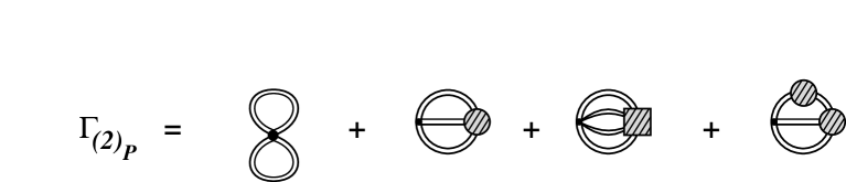
FIG. 4.: The 2-loop contribution $\Gamma^{(2)}_{P}$ , eqs. (34)-(40), to the effective action $\Gamma_{P}$ of eq. (27), in the diagrammatic representation of Fig. 3. Formally, $\Gamma^{(2)}_{P}$ is the sum of all two-particle irreduclible graphs with internal lines representing the full gluon propagators $\widehat{\Delta}$ and full 3- and 4-gluon vertices $\widehat{V}$ and $\widehat{W}$.

C Equations of motion

As scetched above and discussed in more detail in Appendix E, the equations of motion (24) and (25) result from approximating the exact theory by truncation of the infinite hierarchy of equations for the $n$-point Green functions to the 1-point function (the soft mean field $\overline{A}(x)$) and the 2-point function (the hard propagator $i\widehat{\Delta}(x,y)$), with all higher-point functions being combinations of these and connected by the 3-gluon and 4-gluon vertices $-ig\widehat{V}(x,y,z)$ and $-g^{2}\widehat{W}(x,y,z,w)$, respectively. Before writing down the explicit form of the resulting equations of motion, it is useful to summarize the terminology introduced in the course of the above discussion:

• mean field $\overline{A}$ (Fig. 3f): denotes the classical soft field as the expectation value of the gauge field $A$, which is induced by the abundance of emitted hard gluons and their collective motion.

• free propagator $i\Delta_{0}$ (Fig. 3a): refers to the free propagation of hard gluons in the absence of interactions, i.e. vanishing coupling $g=0$.

• mean-field propagator $i\overline{\Delta}$ (Fig. 3b): denotes to the tree-level propagator without quantum corrections, i.e. the free propagator with an arbitrary number $\geq 0$ of attached external legs coupling to the soft mean field, but without closed loops that correspond to quantum self-interactions.

• full propagator $i\widehat{\Delta}$ (Fig. 3c): terms the dressed propagator of the hard quanta, that is renormalized by both the interactions with the soft mean field and the self-interactions among the hard quanta.

• full vertex functions $-ig\widehat{V},\;-g^{2}\widehat{W}$ (Fig. 3d, 3e): represent the 3-gluon and 4-gluon vertices with the internal lines being the full hard propagator including mean-field and quantum interactions.

1 Yang-Mills equation for the soft mean field

The equation of motion for the soft field $\overline{A}_{\mu}^{a}(x)$, is given by (24), i.e., $\delta\Gamma_{P}/\delta\overline{A}=-{\cal K}^{(1)}-{\cal K}^{(2)}\circ\overline{A}$, from which one obtains, upon taking into account the initial condition (26), ${\cal K}^{(1)}=0$, the Yang-Mills equation for $\overline{A}$:

$$\left[\frac{}{}\overline{D}^{\lambda,\;ab},\;\overline{F}_{\lambda\mu}^{b}\right](x)\;=\;-\,\widehat{j}_{\mu}^{a}(x)\;-\;\left(\frac{}{}{\cal K}_{\;\;\;\mu\lambda}^{(2)\,ab}\,\circ\,\overline{A}^{\lambda,\,b}\right)(x)\;,$$ (47)

where $[\overline{D},\overline{F}]=\overline{D}\,\overline{F}-\overline{F}\,\overline{D}$ with the covariant derivative defined as $\overline{D}^{\lambda}\equiv D^{\lambda}[\overline{A}]=\partial_{x}^{\lambda}-ig\overline{A}^{\lambda}(x)$, and $\overline{F}_{\lambda\mu}\equiv F_{\lambda\mu}[\overline{A}]=\left[\overline{D}_{\lambda}\,,\,\overline{D}_{\mu}\right]/(-ig)$. The second term on the right side is the initial state contribution to the current, according to the condition (26), ${\cal K}^{(2)}\circ\overline{A}=\int_{P}d^{4}y\,{\cal K}_{\;\;\;\mu\lambda}^{(2)\,ab}(x,y)\,\overline{A}^{\lambda,\,b}(y)$.

Rewriting the left hand side of (47) as

$$\left[\frac{}{}\overline{D}^{\lambda,\;ab},\;\overline{F}_{\lambda\mu}^{b}\right](x)\;=\;{\cal D}_{0\;\mu\lambda}^{-1\;\;ab}\;\overline{A}^{\lambda,\,b}(x)\;\;+\;\;\overline{\Xi}_{\mu}^{a}(x)\;\;\;\;\;\;\;\;\;\;\;\;\;\;\;{\cal D}_{0\;\mu\lambda}^{-1\;\;ab}\;\equiv\;\delta^{ab}\,\left(g_{\mu\lambda}\partial_{x}^{2}-\partial^{x}_{\mu}\partial^{x}_{\lambda}-n_{\mu}n_{\lambda}\right)\;,$$ (48)

where, upon taking into account the gauge constraint (2), the $-n_{\mu}n_{\lambda}\overline{A}^{\lambda}$ in ${\cal D}_{0\;\mu\lambda}^{-1}\;\overline{A}^{\lambda}$ does not contribute, because $0=\langle n\cdot A\rangle=n^{\nu}\overline{A}_{\nu}$, eq. (47) may be expressed in the alternative form (see Fig. 5a):

$$\left\{\frac{}{}\left({\cal D}_{0}^{-1}\;+\;{\cal K}^{(2)}\,\right)\,\overline{A}\right\}_{\mu}^{a}(x)\;\;+\;\;\overline{\Xi}_{\mu}^{a}(x)\;\;+\;\;\widehat{j}_{\mu}^{a}(x)\;\;=\;\;0\;.$$ (49)

Here the function $\overline{\Xi}$ contains the soft-field self-coupling,

$$\overline{\Xi}_{\mu}^{a}(x)\;\;=\;\;\overline{\Xi}_{(1)\;\mu}^{a}(x)\;\;+\;\;\overline{\Xi}_{(2)\;\mu}^{a}(x)$$ (50)

$$\overline{\Xi}_{(1)\;\mu}^{a}(x) = \;-\;\frac{g}{2}\,\int_{P}\prod_{i=1}^{2}d^{4}x_{i}\;V_{0\;\mu\nu\lambda}^{\;\;\;\;abc}(x,x_{1},x_{2})\;\overline{A}^{\nu,\,b}(x_{1})\overline{A}^{\lambda,\,c}(x_{2})$$ (51)

$$\overline{\Xi}_{(2)\;\mu}^{a}(x) = \;+\;\frac{i\,g^{2}}{6}\,\int_{P}\prod_{i=1}^{3}d^{4}x_{i}\;W_{0\;\mu\nu\lambda\sigma}^{\;\;\;\;abcd}(x,x_{1},x_{2},x_{3})\;\overline{A}^{\nu,\,b}(x_{1})\overline{A}^{\lambda,\,c}(x_{2})\overline{A}^{\sigma,\,d}(x_{3})\;,$$ (52)

and the current $\widehat{j}$ is the induced current due to the hard quantum dynamics in the presence of the soft field $\overline{A}$:

$$\widehat{j}_{\mu}^{a}(x)\;\;=\;\;\widehat{j}_{(1)\;\mu}^{a}(x)\;\;+\;\;\widehat{j}_{(2)\;\mu}^{a}(x)\;\;+\;\;\widehat{j}_{(3)\;\mu}^{a}(x)$$ (53)

$$\widehat{j}_{(1)\;\mu}^{a}(x) = -\;\frac{i\,g}{2}\,\int_{P}\prod_{i=1}^{2}d^{4}x_{i}\;V_{0\;\mu\nu\lambda}^{\;\;\;\;abc}(x,x_{1},x_{2})\;\widehat{\Delta}^{\nu\lambda,\,bc}(x_{1},x_{2})$$ (54)

$$\widehat{j}_{(2)\;\mu}^{a}(x) = -\;\frac{g^{2}}{2}\,\;\int_{P}\prod_{i=1}^{3}d^{4}x_{i}\;\;W_{0\;\mu\nu\lambda\sigma}^{\;\;\;\;abcd}(x,x_{1},x_{2},x_{3})\;\overline{A}^{\nu,\,b}(x_{1})\;\widehat{\Delta}^{\lambda\sigma,\,cd}(x_{2},x_{3})$$ (55)

$$\widehat{j}_{(3)\;\mu}^{a}(x) = -\;\frac{ig^{3}}{6}\,\;\int_{P}\prod_{i=1}^{3}d^{4}x_{i}d^{4}y_{i}\;\;W_{0\;\mu\nu\lambda\sigma}^{\;\;\;\;abcd}(x,x_{1},x_{2},x_{3})\;\widehat{\Delta}^{\nu\nu^{\prime},\,bb^{\prime}}(x_{1},y_{1})\;\widehat{\Delta}^{\lambda\lambda^{\prime},\,cc^{\prime}}(x_{2},y_{2})\;$$ (57)

$$\;\;\;\;\;\;\;\;\;\;\;\;\;\;\;\;\;\;\;\;\;\;\;\;\;\;\;\;\;\;\;\;\;\;\;\;\;\;\;\;\times\;\widehat{\Delta}^{\sigma\sigma^{\prime},\,dd^{\prime}}(x_{3},y_{3})\;\;V_{0\;\mu^{\prime}\nu^{\prime}\lambda^{\prime}\sigma^{\prime}}^{\;\;\;\;abcd}(y_{1},y_{2},y_{3})\;.$$

It should be remarked that the function $\overline{\Xi}$ on the left hand side of (47) contains the non-linear self-coupling of the soft field $\overline{A}$ alone, whereas the induced current $\widehat{j}$ on the right hand side is determined by the hard propagator $\widehat{\Delta}$, thereby generating the soft field.

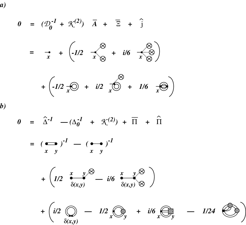
FIG. 5.: Diagrammatic representation in terms of the rules of Fig. 3, of the equations of motion: a) The Yang-Mills equation (47), (48) for the soft field $\overline{A}$ with the self-coupling contribution $\overline{\Xi}$, eqs. (50)-(52) and the generating hard gluon current $\widehat{j}$, eqs. (243)-(247). a) The Dyson-Schwinger equation (58) for the hard propagator $\widehat{\Delta}$ with the mean-field polarization tensor $\overline{\Pi}$, eqs. (59)-(61) and the quantum contribution $\widehat{\Pi}$, eqs. (62)-(68).

2 Dyson-Schwinger equation for the hard gluon propagator

From the equation of motion (25) for the hard propagator, $\widehat{\Delta}_{\mu\nu}^{ab}(x,y)$, that is, $\delta\Gamma_{P}/\delta\widehat{\Delta}={\cal K}^{(2)}/(2i)$, one finds after incorporating condition (26), ${\cal K}^{(1)}=0$, the Dyson-Schwinger equation for $\widehat{\Delta}$ (see Fig. 5b):

$$\left\{\frac{}{}\;\left(\widehat{\Delta}\right)^{-1}\;\;-\;\;\left(\Delta_{0}\right)^{-1}\;\;-\;\;{\cal K}^{(2)}\;\;+\;\;\overline{\Pi}\;\;+\;\;\widehat{\Pi}\;\right\}_{\mu\nu}^{ab}(x,y)\;\;=\;\;0\;,$$ (58)

where $\widehat{\Delta}$ is the fully dressed propagator of the hard quantum fluctuations in the presence of the soft mean field, defined by (32), whereas $\Delta_{0}$ is the free propagator, given by (29). The polarization tensor $\Pi$ has been decomposed in two parts, a mean-field part $\overline{\Pi}$ and a quantum fluctuation part $\widehat{\Pi}$. The mean-field polarization tensor $\overline{\Pi}$ incorporates the local interaction between the hard quanta and the soft mean field,

$$\overline{\Pi}_{\mu\nu}^{ab}(x,y)\;\;=\;\;\overline{\Pi}_{(1)\;\mu\nu}^{\;\;\;\;ab}(x,y)\;\;+\;\;\overline{\Pi}_{(2)\;\mu\nu}^{\;\;\;\;ab}(x,y)$$ (59)

$$\overline{\Pi}_{(1)\;\mu\nu}^{\;\;\;\;ab}(x,y) = \frac{ig}{2}\;\delta_{P}^{4}(x,y)\;\,\int_{P}d^{4}z\,V_{0\;\mu\nu\lambda}^{abc}(x,y,z)\,\overline{A}^{\lambda,\,c}(z)$$ (60)

$$\overline{\Pi}_{(2)\;\mu\nu}^{\;\;\;\;ab}(x,y) = \frac{g^{2}}{6}\;\delta_{P}^{4}(x,y)\;\,\int_{P}d^{4}zd^{4}w\,W_{0\;\mu\nu\lambda\sigma}^{abcd}(x,y,z,w)\,\overline{A}^{\lambda,\,c}(z)\,\overline{A}^{\sigma,\,d}(w)\;.$$ (61)

plus terms of order $g^{3}\overline{A}^{3}$ which one may safely ignore within the present approximation scheme. The fluctuation polarization tensor $\widehat{\Pi}$ contains the quantum self-interaction among the hard quanta in the presence of $\overline{A}$. It is given by the variation $2i\delta\Gamma_{P}^{(2)}/\delta\widehat{\Delta}$ of the 2-loop part $\Gamma_{P}^{(2)}$, eq. (34), of the effective action $\Gamma_{P}$,

$$\widehat{\Pi}^{ab}_{\mu\nu}(x,y)\;\;=\;\;\widehat{\Pi}^{\;\;\;\;ab}_{(1)\;\mu\nu}(x,y)\;\;+\;\;\widehat{\Pi}^{\;\;\;\;ab}_{(2)\;\mu\nu}(x,y)\;\;+\;\;\widehat{\Pi}^{\;\;\;\;ab}_{(3)\;\mu\nu}(x,y)\;\;+\;\;\widehat{\Pi}^{\;\;\;\;ab}_{(4)\;\mu\nu}(x,y)\;,$$ (62)

$$\widehat{\Pi}^{\;\;\;\;ab}_{(1)\;\mu\nu}(x,y) = -\,\frac{g^{2}}{2}\;\int_{P}d^{4}x_{1}d^{4}y_{1}\;\;W_{0\;\mu\nu\lambda\sigma}^{\;\;\;\;abcd}(x,y,x_{1},y_{1})\;\widehat{\Delta}^{\lambda\sigma\,,cd}(y_{1},x_{1})\;$$ (63)

$$\widehat{\Pi}^{\;\;\;\;ab}_{(2)\;\mu\nu}(x,y) = -\,\frac{i\,g^{2}}{2}\;\int_{P}\prod_{i=1}^{2}d^{4}x_{i}d^{4}y_{i}\;\;V_{0\;\mu\lambda\sigma}^{\;\;\;\;acd}(x,x_{1},x_{2})\;\;\widehat{\Delta}^{\lambda\lambda^{\prime},\,cc^{\prime}}(x_{1},y_{1})\;\widehat{\Delta}^{\sigma\sigma^{\prime},\,dd^{\prime}}(x_{2},y_{2})\;\widehat{V}_{\sigma^{\prime}\lambda^{\prime}\nu}^{d^{\prime}c^{\prime}b}(y_{2},y_{1},y)$$ (64)

$$\widehat{\Pi}^{\;\;\;\;ab}_{(3)\;\mu\nu}(x,y) = -\;\frac{g^{4}}{6}\;\int_{P}\prod_{i=1}^{3}d^{4}x_{i}d^{4}y_{i}\;\;W_{0\;\mu\lambda\sigma\tau}^{\;\;\;\;acde}(x,x_{1},x_{2},x_{3})\;\;\widehat{\Delta}^{\lambda\lambda^{\prime},\,cc^{\prime}}(x_{1},y_{1})\;\widehat{\Delta}^{\sigma\sigma^{\prime},\,dd^{\prime}}(x_{2},y_{2})\;$$ (66)

$$\;\;\;\;\;\;\;\;\;\;\;\;\;\;\;\;\;\;\;\;\;\;\;\;\;\;\;\;\;\;\;\;\;\;\;\;\;\;\;\;\;\;\;\;\;\;\;\;\;\;\;\;\;\;\;\;\times\;\widehat{\Delta}^{\tau\tau^{\prime},\,ee^{\prime}}(x_{3},y_{3})\;\widehat{W}_{\tau^{\prime}\sigma^{\prime}\lambda^{\prime}\nu}^{e^{\prime}d^{\prime}c^{\prime}b}(y_{3},y_{2},y_{1},y)$$

$$\widehat{\Pi}^{\;\;\;\;ab}_{(4)\;\mu\nu}(x,y) = -\;\frac{i\,g^{4}}{24}\;\int_{P}\prod_{i=1}^{2}d^{4}x_{i}d^{4}y_{i}d^{4}z_{i}\;\;W_{0\;\mu\lambda\sigma\tau}^{\;\;\;\;acde}(x,x_{1},x_{2},x_{3})\;\;\widehat{\Delta}^{\sigma\rho^{\prime},\,df^{\prime}}(x_{2},z_{2})\;\widehat{\Delta}^{\tau\rho^{\prime\prime},\,ef^{\prime\prime}}(x_{3},z_{3})\;$$ (68)

$$\;\;\;\;\;\;\;\;\;\;\;\;\;\;\;\;\;\;\;\;\;\;\;\;\;\;\;\;\;\;\;\times\;\widehat{V}_{\rho^{\prime\prime}\rho^{\prime}\rho}^{f^{\prime\prime}f^{\prime}f}(z_{3},z_{2},z_{1})\;\;\widehat{\Delta}^{\rho\lambda^{\prime},\,fc^{\prime}}(z_{1},y_{1})\;\widehat{\Delta}^{\lambda\sigma^{\prime},\,cd^{\prime}}(x_{1},y_{2})\;\;\;\widehat{V}_{\lambda^{\prime}\sigma^{\prime}}^{c^{\prime}d^{\prime}}(y_{1},y_{2},y)\;.$$

Note that the usual Dyson-Schwinger equation in vacuum is contained in (58) -(68) as the special case when the mean field vanishes, $\overline{A}(x)=0$, and initial state correlations are absent, ${\cal K}^{(2)}(x,y)=0$. In this case, the propagator becomes the usual vacuum propagator, since the mean-field contribution $\overline{\Pi}$ is identically zero, and the quantum part $\widehat{\Pi}$ reduces to the vacuum contribution.

III TRANSITION TO QUANTUM KINETICS

The equations of motion (47) or (49) for $\overline{F}_{\mu\nu}$ or $\overline{A}_{\mu}$, and (58) for $\widehat{\Delta}_{\mu\nu}$, are non-linear integro-differential equations and clearly not solvable in all their generality. However, the field-equations of motion (47) or (58) can be cast into much simpler quantum-kinetic equations with the help of the Wigner-function technique and gradient expansion, and the assumption of 2-scale separation. As a result one obtains finally the three master equations mentionened in Sec. 1: a simplified Yang-Mills equation decribing the space-time change of $\overline{A}$, and two equations for the gluon propagator $\widehat{\Delta}$, namely, first, an evolution equation for the QCD evolution in momentum space, and second, a transport equation for the space-time development in the presence of $\overline{A}$. In order to achieve this result, one needs to make a third key approximation (in addition to the two approximations of Sec. II A), namely,

• approximation 3: It is assumed that the induced soft field $\overline{A}_{\mu}$ is slowly varying on the scale of the short-range, hard quantum fluctuations, that is, the gradient of the soft field is small compared to the Compton wavelength of the hard quanta. Then one can treat the quantum fluctuations of $\widehat{\Delta}(r,k)$ at short distances separately from the collective effects represented by to the soft field $\overline{A}(r)$ with long wavelength.

A Quantum and kinetic space-time regimes

The key to derive from (47) or (58) the corresponding approximate quantum-kinetic equations is the separability of hard and soft dynamics in terms of the space-time scale $\lambda\equiv 1/\mu$, where $\mu$ is the parametric momentum scale introduced in (6). This implies that one may characterize the dynamical evolution of the gluon system by a short-range quantum scale $r_{qua}\ll\lambda$, and a comparably long-range kinetic scale $r_{kin}\,\lower 3.0pt\hbox{$\buildrel>\over{\sim}$}\,\lambda$. Low-momentum collective excitations that may develop at the particular momentum scale $g\mu$ are thus well separated from the typical hard gluon momenta $k_{\perp}\geq\mu$, if $g\ll 1$. Therefore, collectivity can arise, because the wavelength of the soft oscillations $\sim 1/g\mu$ is much larger than the typical extention of the hard quantum fluctuations $\sim 1/\mu$. I emphasize that this notion of two characteristic scales is not just an academic construction, but rather is a typical property of quantum field theory. A simple example is a freely propagating electron: In this case, the quantum scale is given its the Compton wavelength $\sim 1/m_{e}$ in the restframe of the charge, and measures the size of the radiative vacuum polarization cloud around the bare charge. The kinetic scale, on the other hand, is determined by the mean-free-path of the charge, which is infinite in vacuum, and in medium is inversely proportional to the local charge density times the interaction cross-section, $\sim 1/(n_{e}\,\sigma_{int})$. Adopting this notion to the present case of gluon dynamics, I define $r_{qua}$ and $r_{kin}$ as follows:

• The quantum scale $r_{qua}$ measures the spatial extension of quantum fluctuations associated with virtual and real radiative emission and re-absorption off a given hard gluon, described by the hard propagator $\widehat{\Delta}$. It can thus be interpreted as its Compton wavelength, corresponding to the typical transverse extension of the fluctuations and thus inversely proportional to the average transverse momentum,

  $$r_{qua}\;\,\equiv\;\,\widehat{\lambda}\;\;\simeq\;\;\frac{1}{\langle\;k_{\perp}\;\rangle}\;,\;\;\;\;\;\;\;\;\;\;\;\;\;\;\;\langle\;k_{\perp}\;\rangle\;\geq\;\mu\;,$$ (69)

  where the second relation is imposed by means of the definition (6) of hard and soft modes. In general, $\widehat{\lambda}$ can be space-time dependent quantity, because the magnitude of $\langle k_{\perp}\rangle$ is determined by both the radiative self-interactions of the hard gluons and ther interactions with the soft field.

• The kinetic scale $r_{kin}$ measures the range of the long-wavelength correlations, described by the soft mean-field $\overline{A}$, and may be parametrized in terms of the average transverse wavelength of soft modes $\langle q_{\perp}\rangle$, such that

  $$r_{kin}\;\,\equiv\;\,\overline{\lambda}\;\;\simeq\;\;\frac{1}{\langle\;q_{\perp}\;\rangle}\;,\;\;\;\;\;\;\;\;\;\;\;\;\;\;\;\langle\;q_{\perp}\;\rangle\;\,\lower 3.0pt\hbox{$\buildrel<\over{\sim}$}\,\;g\,\mu\;,$$ (70)

  where $\overline{\lambda}$ may vary from one space-time point to another, because the population of soft modes $\overline{A}(q)$ is determined locally by the hard current $\widehat{j}$ with dominant contribution from gluons with transverse momentum $\simeq\mu$.

The above classification of quantum- (kinetic-) scales specifies in space-time the relevant regime for the hard (soft) dynamics, so that the separability of the two scales $r_{qua}$ and $r_{kin}$ imposes the following condition on the relation between space-time and momentum:

$$\widehat{\lambda}\;\;\ll\;\;\overline{\lambda}\;,\;\;\;\;\;\;\;\;\;\;\;\;\;\mbox{or}\;\;\;\;\;\;\;\;\;\;\;\;\;\;\langle\;k_{\perp}\;\rangle\;\;\;\geq\;\mu\;\;\gg\;\;g\,\mu\;\;\approx\;\;\;\langle\;q_{\perp}\;\rangle\;.$$ (71)

The physical interpretation of (71) is simple: At short distances $r_{qua}\ll 1/(g\mu)$ a hard gluon can be considered as an incoherent quantum which emits and partly reabsorbs daughter gluons, corresponding to the combination of real brems-strahlung and virtual radiative fluctuatiuons. Only a hard probe with a short wavelength $\widehat{\lambda}\leq r_{qua}$ can resolve this quantum dynamics. On the other hand, at larger distances $r_{kin}\approx 1/(g\mu)$, a gluon appears as a coherent quasi-particle, that is, as an extended object with a changing transverse size corresponding to the extent of its intrinic quantum fluctuations. This dynamical substructure is however not resolvable by long-wavelength modes $\overline{\lambda}\geq r_{kin}$ of the soft field $\overline{A}$.

Accordingly, one may classify the quantum and kinetic regimes, respectively, by associating with two distinct space-time points $x^{\mu}$ and $y^{\mu}$ the following characteristic scales:

$$s^{\mu}\; \equiv \;\;\;\;\;\;x^{\mu}\;-\;y^{\mu}\;\;\;\;\;\sim\;\widehat{\lambda}\;=\;\frac{1}{g\mu}\;,\;\;\;\;\;\;\;\;\;\;\;\;\;\partial_{s}^{\mu}\;=\;\frac{1}{2}\;\left(\partial_{x}^{\mu}\;-\;\partial_{y}^{\mu}\right)\;\;\sim\;\;g\,\mu$$ (72)

$$r^{\mu}\; \equiv \frac{1}{2}\;\left(x^{\mu}\;+\;y^{\mu}\right)\;\;\;\;\sim\;\overline{\lambda}\;=\;\frac{1}{\mu}\;,\;\;\;\;\;\;\;\;\;\;\;\;\;\;\;\partial_{r}^{\mu}\;=\;\;\;\;\;\partial_{x}^{\mu}\;+\;\partial_{y}^{\mu}\;\;\;\;\sim\;\;\;\mu\;.$$ (73)

On the kinetic scale the effect of the soft field modes of $\overline{A}$ on the hard quanta involves the coupling $g\overline{A}$ to the hard propapgator and is of the order of the soft wavelength $\overline{\lambda}=1/(g\mu)$, so that one may characterize the soft field strength by

$$g\overline{A}_{\mu}(r)\;\;\sim\;\;g\mu\;,\;\;\;\;\;\;\;\;\;\;\;\;g\overline{F}_{\mu\nu}(r)\;\;\sim\;\;g^{2}\,\mu^{2}\;,$$ (74)

plus corrections of order $g^{2}\mu^{2}$ and $g^{3}\mu^{3}$, respectively, which are assumed to be small.

On the quantum scale, on the other hand,

$$\widehat{\Delta}_{\mu\nu}^{-1}\;\;\sim k_{\perp}^{2}\;\,\lower 3.0pt\hbox{$\buildrel>\over{\sim}$}\,\;\mu^{2}\;\;\gg\;\;g^{2}\mu^{2}\;\;\sim\;\;g\,\overline{F}_{\mu\nu}\;,$$ (75)

and one expects that that the short-distance fluctuations corresponding to emission and reabsorption of gluons with momenta $k_{\perp}\geq\mu$, are little affected by the long-range, soft mean field, because the color force $\sim g\overline{F}$ acting on a gluon with momentum $k_{\perp}\sim\mu$ produces only a very small change in its momentum.

B The kinetic approximation

The realization of the two space-time scales, short-distance quantum and quasi-classical kinetic, allows to reformulate the quantum field-theoretical problem as a relativistic many-body problem within kinetic theory. The key element is to establish the connection between the preceding description in terms of Green functions and a probabilistic kinetic description in terms of of so-called Wigner functions [31]. Whereas the 2-point functions, such as the propagator or the polarization tensor, depend on two separate space-time points $x$ and $y$, their Wigner transforms utilizes a mixed space-time/momentum representation, which is particularly convenient for implementing the assumption of separated quantum and kinetic scales, i.e., that the long-wavelength field $\overline{A}$ is slowly varying in space-time on the scale of short-range quantum fluctuations. Moreover, the trace of the Wigner-transformed propagator is the quantum analogue of the single particle phase-space distribution of gluons, and therefore provides the basic quantity to make contact with kinetic theory of multi-particle dynamics [18].

In terms of the center-of-mass coordinate, $r=\frac{1}{2}(x+y)$, and relative coordinate $s=x-y$, of two space-time points $x$ and $y$, eq. (73), one can express any 2-point function ${\cal G}(x,y)$, such as $\widehat{\Delta},\Pi$, in terms of these coordinates,

$${\cal G}_{\mu\nu}^{ab}(x,y)\;=\;{\cal G}_{\mu\nu}^{ab}\left(r+\frac{s}{2},r-\frac{s}{2}\right)\;\;\equiv\;\;{\cal G}_{\mu\nu}^{ab}\left(r,s\right)\;,\;\;\;\;\;\;\;\;\;\;\;\;\;\;.$$ (76)

The Wigner transform ${\cal G}(r,k)$ is then defined as the Fourier transform with respect to the relative coordinate $s$, being the canonical conjugate to the momentum $k$. In general, the necessary preservation of local gauge symmetry requires a careful definition that obeys the gauge transformation properties [7], but for the specific choice of gauge (2), the Wigner transform is simply [32]:

$${\cal G}(r,s)\;=\;\int\frac{d^{4}k}{(2\pi)^{4}}\,e^{-i\,k\,\cdot\,s}\;\,{\cal G}\left(r,k\right)\;\;,\;\;\;\;\;\;\;\;\;\;\;\;\;{\cal G}\left(r,k\right)\;=\;\int d^{4}s\,e^{i\,k\,\cdot\,s}\;\,{\cal G}\left(r,s\right)\;.$$ (77)

The Wigner representation (77) will facilitate a systematic identification of the dominant contributions of the soft field $\overline{A}$ to the hard propagator $\widehat{\Delta}$, a concept that has been developed by Blaizot and Iancu [7]: First, one expands both $\overline{A}$ and $\widehat{\Delta}=\widehat{\Delta}_{[\overline{0}]}+\delta\widehat{\Delta}_{[\overline{A}]}$ in terms of gradients of the long-range variation with the kinetic scale $r$, and second, one makes an additional expansion in powers of the soft field $\overline{A}$ and of the induced perturbation $\delta\widehat{\Delta}_{[\overline{A}]}\sim g\widehat{\Delta}_{[\overline{0}]}$.

1 Gradient expansion

To proceed, recall that the coordinate $r^{\mu}$ describes the kinetic space-time dependence $\sim r_{kin}$, whereas $s$ measures the quantum space-time distance $\sim r_{qua}$. In translational invariant situations, e.g. in vacuum or thermal equilibrium, ${\cal G}(r,s)$ in (77) is independent of $r^{\mu}$ and sharply peaked about $s^{\mu}=0$. Here the range of the variation is fixed by $\lambda=1/\mu$, eq. (69), corresponding to the confinement length $const.\times 1/\Lambda$ in the case of vacuum, or to the thermal wavelength $const.\times 1/T$ in equilibrium. On the other hand, in the presence of a slowly varying soft field $\overline{A}$ with a wavelength $\overline{\lambda}=1/(g\mu)$, eq. (70), the $s^{\mu}$ dependence is little affected, while the acquired $r^{\mu}$ dependence will have a long-wavelength variation. In view of the estimates (73), one may therefore neglect the derivatives of ${\cal G}(r,k)$ with respect to $r^{\mu}$ which are of order $g\mu$, relative to those with respect to $s^{\mu}$ which are of order $\mu$.

Hence one can perform the so-called gradient expansion of the soft field and the hard propagator and polarization tensor in terms of gradients $(s\cdot\partial_{r})^{n}$, and keep only terms up to first order $n=1$, i.e.,

$$\overline{A}_{\mu}(x)\;=\;\overline{A}_{\mu}\left(r+\frac{s}{2}\right)\;\simeq\;\overline{A}_{\mu}(r)+\frac{s}{2}\cdot\partial_{r}\overline{A}_{\mu}(r)\;,$$ (78)

and similarly for $\overline{A}_{\mu}(y)=\overline{A}_{\mu}(r-s/2)$, as well as

$$\widehat{\Delta}_{\mu\nu}\left(x,y\right) = \widehat{\Delta}_{\mu\nu}\left(r,s\right)\;\simeq\;\widehat{\Delta}_{\mu\nu}\left(0,s\right)\;+\;s\,\cdot\,\partial_{r}\,\widehat{\Delta}_{\mu\nu}\left(r,s\right)$$ (79)

$$\widehat{\Pi}_{\mu\nu}\left(x,y\right) = \widehat{\Pi}_{\mu\nu}\left(r,s\right)\;\simeq\;\widehat{\Pi}_{\mu\nu}\left(0,s\right)\;+\;s\,\cdot\,\partial_{r}\,\widehat{\Pi}_{\mu\nu}\left(r,s\right)\;,$$ (81)

Then, by using the following conversion rules [11, 23] to carry out the Wigner transformations,

$$\int d^{4}x^{\prime}f(x,x^{\prime})\,g(x^{\prime},y)\;\Rightarrow\;f(r,k)\,g(r,k)\, + \,\frac{i}{2}\;\left[(\partial_{k}f)\cdot(\partial_{r}g)\;-\;(\partial_{r}f)\cdot(\partial_{k}g)\right]$$ (82)

$$h(x)\,g(x,y)\;\Rightarrow\;h(r)\,g(r,k)\;-\;\frac{i}{2}\,(\partial_{r}h)\cdot(\partial_{k}g)\;\;\; \;\;\;h(y)\,g(x,y)\;\Rightarrow\;h(r)\,g(r,k)\;+\;\frac{i}{2}\,(\partial_{r}h)\cdot(\partial_{k}g)$$ (83)

$$\partial_{x}^{\mu}f(x,y)\;\Rightarrow\;(-ik^{\mu}\,+\,\frac{1}{2}\partial_{r}^{\mu})\,f(r,k)\;\;\; \;\;\;\partial_{y}^{\mu}f(x,y)\;\Rightarrow\;(+ik^{\mu}\,+\,\frac{1}{2}\partial_{r}^{\mu})\,f(r,k)\;,$$ (84)

the transformed polarization tensor $\Pi(r,k)$ is obtained from $\Pi(x,y)$, eqs. (59) and (62), with

$$\Pi_{\mu\nu}(r,k)=\overline{\Pi}_{\mu\nu}(r,k)+\widehat{\Pi}_{\mu\nu}(r,k)$$ (85)

where the soft mean-field contribution [c.f. (60), (61)] is

$$\overline{\Pi}_{\mu\nu}^{ab}(r,k)\;\;=\;\;\left(\frac{}{}\overline{\Pi}_{(1)}\;+\;\overline{\Pi}_{(2)}\right)_{\mu\nu}^{ab}(r,k)$$ (86)

$$\overline{\Pi}_{(1)\;\mu\nu}^{\;\;\;\;ab}(r,k) = \frac{ig}{2}\,V_{0\;\mu\nu\lambda}^{abc}(k,0,-k)\,\overline{A}^{\lambda,\,c}(r)$$ (87)

$$\overline{\Pi}_{(2)\;\mu\nu}^{\;\;\;\;ab}(r,k) = \;-\;\frac{ig}{6}\,W_{0\;\mu\nu\lambda\sigma}^{abcd}(k,0,0,-k)\,\overline{A}^{\lambda,\,c}(r)\,\overline{A}^{\sigma,\,d}(r)\;,$$ (88)

and the quantum contribution [c.f. (62)-(68)] is

$$\widehat{\Pi}_{\mu\nu}^{ab}(r,k)\;\;=\;\;\left(\frac{}{}\widehat{\Pi}_{(1)}\;+\;\widehat{\Pi}_{(2)}\;+\;\widehat{\Pi}_{(3)}\;+\;\widehat{\Pi}_{(4)}\right)_{\mu\nu}^{ab}(r,k)$$ (89)

$$\widehat{\Pi}^{\;\;\;\;ab}_{(1)\;\mu\nu}(r,k) = +\,\frac{ig^{2}}{2}\;\int\frac{d^{4}q}{(2\pi)^{4}\;i}\;\;W_{0\;\mu\nu\lambda\sigma}^{\;\;\;\;abcd}(k,q,-q,-k)\;\widehat{\Delta}^{\lambda\sigma\,,cd}(r,k)\;$$ (90)

$$\widehat{\Pi}^{\;\;\;\;ab}_{(2)\;\mu\nu}(r,k) = +\,\frac{g^{2}}{2}\;\int\frac{d^{4}q}{(2\pi)^{4}\;i}\;\;V_{0\;\mu\lambda\sigma}^{\;\;\;\;acd}(k,-q,-q^{\prime})\;\;\widehat{\Delta}^{\lambda\lambda^{\prime},\,cc^{\prime}}(r,q)\;\widehat{\Delta}^{\sigma\sigma^{\prime},\,dd^{\prime}}(r,q^{\prime})\;\widehat{V}_{\sigma^{\prime}\lambda^{\prime}\nu}^{d^{\prime}c^{\prime}b}(r;q^{\prime},q,-k)$$ (91)

$$\widehat{\Pi}^{\;\;\;\;ab}_{(3)\;\mu\nu}(r,k) = -\;\frac{g^{4}}{6}\;\int\frac{d^{4}q}{(2\pi)^{4}\;i}\frac{d^{4}p}{(2\pi)^{4}\;i}\;\;W_{0\;\mu\lambda\sigma\tau}^{\;\;\;\;acde}(k,-q,-q^{\prime},-p)\;\;\widehat{\Delta}^{\lambda\lambda^{\prime},\,cc^{\prime}}(r,q)\;\widehat{\Delta}^{\sigma\sigma^{\prime},\,dd^{\prime}}(r,q^{\prime})\;$$ (93)

$$\;\;\;\;\;\;\;\;\;\;\;\;\;\;\;\;\;\;\;\;\;\;\;\;\;\;\;\;\;\;\;\;\;\;\;\;\;\;\;\;\;\;\;\;\;\;\;\;\;\;\;\;\;\;\;\;\times\;\widehat{\Delta}^{\tau\tau^{\prime},\,ee^{\prime}}(r,p)\;\widehat{W}_{\tau^{\prime}\sigma^{\prime}\lambda^{\prime}\nu}^{e^{\prime}d^{\prime}c^{\prime}b}(r;q,q^{\prime},p,-k)$$

$$\widehat{\Pi}^{\;\;\;\;ab}_{(4)\;\mu\nu}(r,k) = -\;\frac{g^{4}}{24}\;\int\frac{d^{4}q}{(2\pi)^{4}\;i}\frac{d^{4}p}{(2\pi)^{4}\;i}\;\;W_{0\;\mu\lambda\sigma\tau}^{\;\;\;\;acde}(k,-q,-q^{\prime},-p^{\prime})\;\;\widehat{\Delta}^{\sigma\rho^{\prime},\,df^{\prime}}(r,q)\;\widehat{\Delta}^{\tau\rho^{\prime\prime},\,ef^{\prime\prime}}(r,q^{\prime})\;$$ (95)

$$\;\;\;\;\;\;\;\;\;\;\;\;\;\;\;\;\;\;\;\;\;\;\;\;\;\;\;\;\;\;\;\times\;\widehat{V}_{\rho^{\prime\prime}\rho^{\prime}\rho}^{f^{\prime\prime}f^{\prime}f}(r;q,q^{\prime},-p)\;\;\widehat{\Delta}^{\rho\lambda^{\prime},\,fc^{\prime}}(r,p)\;\widehat{\Delta}^{\lambda\sigma^{\prime},\,cd^{\prime}}(r,p^{\prime})\;\;\;\widehat{V}_{\lambda^{\prime}\sigma^{\prime}}^{c^{\prime}d^{\prime}}(r;p,p^{\prime},-k)\;.$$

Here the 3- and 4-gluon vertex functions from (42), (44) and (46) depend explicitly on $r$,

$$\widehat{V}(r;k_{i})=V_{0}(k_{i})+O\left(g^{4}f(r,k_{i})\right)\;\;\;\;\;\;\;\;\;\;\;\;\;\;\;\;\widehat{W}(r;k_{i})=W_{0}(k_{i})+O\left(g^{4}f(r,k_{i})\right)$$ (96)

with the bare point-like vertices $V_{0}$, $W_{0}$ being $r$-independent and given by

$$V_{0\;\lambda\mu\nu}^{abc}(k_{1},k_{2},k_{3}) = -\,i\,f^{abc}\,\left\{\frac{}{}g_{\lambda\mu}(k_{1}-k_{2})_{\nu}\;+\;g_{\mu\nu}(k_{2}-k_{3})_{\lambda}\;+\;g_{\nu\lambda}(k_{3}-k_{2})_{\mu}\right\}$$ (97)

$$W_{0\;\lambda\mu\nu\sigma}^{abcd}(k_{1},k_{2},k_{3},k_{4}) = -\;\left\{\frac{}{}\left(f^{ace}f^{bde}-f^{ade}f^{cbe}\right)\,g_{\lambda\mu}g_{\nu\sigma}\;+\;\left(f^{abe}f^{cde}-f^{ade}f^{bce}\right)\,g_{\lambda\nu}g_{\mu\sigma}\right.$$ (99)

$$\left.\frac{}{}\;\;\;\;\;\;\;\;\;\;\;\;\;\;\;\;\;\;\;\;\;\;\;+\;\left(f^{ace}f^{dbe}-f^{abe}f^{cde}\right)\,g_{\lambda\sigma}g_{\nu\mu}\right\}\;.$$

With the above formulae, one can now convert both the Yang-Mills equation (47) and the Dyson-Schwinger equation (58) into a set of much simpler equations. For the Dyson-Schwinger equation, the Wigner transformation together with the gradient expansion yields two distinct equations for the hard propagator $\widehat{\Delta}^{\mu\nu}(r,k)$, namely, (i) an evolution equation , and (ii) a transport equation. They are obtained [11, 23] by taking the sum and difference of Wigner-transform of (58) and its adjoint, using the rules (82)-(84),

(i) evolution equation:

$$(ii) \;\;\;\left(k^{2}-\frac{1}{4}\partial_{r}^{2}\right)\;\widehat{\Delta}^{\mu\nu}(r,k)\;\;-\;\frac{1}{2}\;\left\{\overline{\Pi}^{\mu}_{\sigma}\,,\,\widehat{\Delta}^{\sigma\nu}\right\}(r,k)\;+\;\frac{i}{4}\;\left[\partial^{\lambda}_{r}\overline{\Pi}^{\mu}_{\sigma}\,,\partial_{\lambda}^{k}\widehat{\Delta}^{\sigma\nu}\right](r,k)$$ (101)

$$\;\;\;\;\;\;\;\;\;\;\;\;\;\;\;\;\;\;\;\;\;\;=\;\;\,d^{\mu\nu}(k)\,\,\hat{1}_{P}\;+\;\frac{1}{2}\;\left\{\widehat{\Pi}^{\mu}_{\sigma}\,,\,\widehat{\Delta}^{\sigma\nu}\right\}(r,k)\;+\;\frac{i}{4}\;\left[\partial^{\lambda}_{k}\widehat{\Pi}^{\mu}_{\sigma}\,,\partial_{\lambda}^{r}\widehat{\Delta}^{\sigma\nu}\right](r,k)\;-\;\frac{i}{4}\;\left[\partial^{\lambda}_{r}\widehat{\Pi}^{\mu}_{\sigma}\,,\partial_{\lambda}^{k}\widehat{\Delta}^{\sigma\nu}\right](r,k)$$

(ii) transport equation:

$$\;\;\;\;\;\;\left(k\cdot\partial_{r}\right)\;\;\widehat{\Delta}^{\mu\nu}(r,k)\;\;+\;\frac{i}{2}\;\left[\overline{\Pi}^{\mu}_{\sigma}\,,\,\widehat{\Delta}^{\sigma\nu}\right](r,k)\;-\;\frac{1}{4}\;\left\{\partial^{\lambda}_{r}\overline{\Pi}^{\mu}_{\sigma}\,,\partial_{\lambda}^{k}\widehat{\Delta}^{\sigma\nu}\right\}(r,k)$$ (102)

$$\;\;\;\;\;\;\;\;\;\;\;\;\;\;\;\;\;\;\;\;\;\;=\;\;-\;\frac{i}{2}\;\left[\widehat{\Pi}^{\mu}_{\sigma}\,,\,\widehat{\Delta}^{\sigma\nu}\right](r,k)\;+\;\frac{1}{4}\;\left\{\partial^{\lambda}_{k}\widehat{\Pi}^{\mu}_{\sigma}\,,\partial_{\lambda}^{r}\widehat{\Delta}^{\sigma\nu}\right\}(r,k)\;-\;\frac{1}{4}\;\left\{\partial^{\lambda}_{r}\widehat{\Pi}^{\mu}_{\sigma}\,,\partial_{\lambda}^{k}\widehat{\Delta}^{\sigma\nu}\right\}(r,k)\;,$$ (103)

where $\partial_{r}^{2}\equiv\partial_{r}\cdot\partial_{r}$, $[A,B]\equiv AB-BA$, $\{A,B\}\equiv AB+BA$. In (101) and (103), $\hat{1}_{P}=1\;(0)$ for $\widehat{\Delta}^{F},\widehat{\Delta}^{\overline{F}}$ ($\widehat{\Delta}^{>},\widehat{\Delta}^{<}$) arises as the transform of $\delta^{4}_{P}(x,y)$. The function $d_{\mu\nu}(k)$ is the sum over the gluon polarizations $s$, (emerging from the Fourier transform of the operator (30)),

$$d_{\mu\nu}(k)\;=\;\sum_{s=1,2}\,\varepsilon_{\mu}(k,s)\cdot\varepsilon_{\nu}^{\ast}(k,s)\;=\;g_{\mu\nu}-\frac{n_{\mu}k_{\nu}+n_{\nu}k_{\mu}}{n\cdot k}\;+\;(n^{2}\,+\,\alpha\,k^{2})\,\frac{k_{\mu}k_{\nu}}{(n\cdot k)^{2}}\;.$$ (104)

with the properties $d_{\mu}^{\mu}(k)=2$ , $k_{\mu}d^{\mu\nu}(k)\stackrel{{\scriptstyle k^{2}\rightarrow 0}}{{\longrightarrow}}0$ and $n_{\mu}d^{\mu\nu}=0=d^{\mu\nu}n_{\nu}$. Furthermore, the initial state contribution ${\cal K}^{(2)}$ appearing in (47) and (58), which contributes only at $r^{0}=t_{0}$, has been absorbed into the hard propagator,

$$\widehat{\Delta}_{\mu\nu}^{-1}(r,k)\;\;\equiv\;\;\widehat{\Delta}_{\mu\nu}^{-1}(r,k)\;\;-\;\;{\cal K}^{(2)}_{\mu\nu}(r,k)\;\delta(r^{0}-t_{0})\;.$$ (105)

For the Yang-Mills equation (47), determining $\overline{F}^{\mu\nu}(r)$, one obtains on the same level of approximation a compact expression in terms of the hard current $\widehat{j}$ :

$$\;\;\;\left[\frac{}{}\overline{D}^{\lambda,\;ab},\;\overline{F}_{\lambda\mu}^{b}\right](r)\;\;=\;\;-\;\widehat{j}_{\mu}^{a}(r)\;\;=\;\;-\,g\,\gamma^{\mu\nu\lambda\sigma}\;\int\frac{d^{4}k}{(2\pi)^{2}}\;\mbox{Tr}\left\{\;T^{a}\,\left(k_{\lambda}\,\widehat{\Delta}_{\nu\sigma}(r,k)\;+\;\frac{i}{2}\left[\overline{D}_{\lambda}^{r},\widehat{\Delta}_{\nu\sigma}(r,k)\right]\right)\right\}\;,$$ (106)

where $\gamma_{\mu\nu\lambda\sigma}\;=\;2\,g_{\mu\nu}\,g_{\lambda\sigma}\;-\;g_{\mu\lambda}\,g_{\nu\sigma}\;-\;g_{\mu\sigma}\,g_{\nu\lambda}$ and $\overline{D}_{\lambda}^{r}=\partial_{\lambda}^{r}-ig\overline{A}_{\lambda}(r)$.

2 Expansion in powers of $g\overline{A}$

In order to isolate the leading effects of the soft mean field $\overline{A}$ on the hard quantum propagator $\widehat{\Delta}$, I follow Ref. [7] to separate the quantum contribution from the mean field contribution on the basis of the assumption that the $\overline{A}$ field is slowly varying on the short-range scale of the quantum fluctuations. To do so, recall eq. (32),

$$\widehat{\Delta}(r,k)\;\;\equiv\;\;\widehat{\Delta}_{[\overline{0}]}(r,k)\;\,+\;\,\delta\widehat{\Delta}_{[\overline{A}]}(r,k)$$ (107)

with the quantum piece $\widehat{\Delta}_{[\overline{0}]}$ and the mean-field part $\delta\widehat{\Delta}_{[\overline{A}]}$ defined by

$$\widehat{\Delta}_{[\overline{0}]}^{\;-1}\;=\;\left.\widehat{\Delta}^{-1}\right|_{\overline{A}=0}\;=\;\Delta_{0}^{-1}\;-\;\left.\widehat{\Pi}\right|_{\overline{A}=0}\;\;\;\;\;\;\;\;\;\;\;\;\;\;\;\;\;\;\delta\widehat{\Delta}_{[\overline{A}]}^{-1}\;=\;\overline{\Delta}^{\,-1}\;-\;\Delta_{0}^{-1}\;=\;-\;\overline{\Pi}\;,$$ (108)

and the free-field propagator ${\Delta}_{0}$ and the mean-field proagator $\overline{\Delta}$ are given by (29) and (31), respectively. Given the ansatz (107), with the feedback of the induced soft field to the hard propagator being contained in $\delta\widehat{\Delta}_{[\overline{A}]}$, the latter is now be expanded in powers of the soft field coupling $g\overline{A}$, and it is anticipated that the mean-field induced part $\delta\widehat{\Delta}_{[\overline{A}]}$, is a correction being at most $g$ times the quantum piece $\widehat{\Delta}_{[\overline{0}]}$, that is,

$$\delta\widehat{\Delta}_{[\overline{A}]}(r,k)\;=\;\sum_{n=1,\infty}\frac{1}{n!}\,\left(g\overline{A}(r)\cdot\partial_{k}\right)^{n}\widehat{\Delta}_{[\overline{0}]}(k)\;\;\simeq\;\;g\overline{A}(r)\cdot\partial_{k}\widehat{\Delta}_{[\overline{0}]}(r,k)\;,$$ (109)

and, to the same order of approximation,

$$\partial_{r}^{\mu}\delta\widehat{\Delta}_{[\overline{A}]\,\mu\nu}(r,k)\;\simeq\;g(\partial_{r}^{\mu}\overline{A}^{\lambda})\partial_{k}^{\lambda}\widehat{\Delta}_{[\overline{0}]\;\mu\nu}(r,k)\;,$$ (110)

where, on the right side, the space-time derivative acts only on $\overline{A}$. Now the decomposition (107) with the approximation (109) is inserted into eqs. (101), (103), (106), and all terms up to order $g^{2}\mu^{2}\widehat{\Delta}_{[\overline{0}]}$ are kept. The resulting equations can be compactly expressed in terms of the kinetic momentum $K_{\mu}$ rather than the canonical momentum $k_{\mu}$ (as always in the context of interactions with a gauge field [33]), which for the class of axial-type gauges (2) amounts to the replacements

$$k_{\mu}\;\longrightarrow\;K_{\mu}\;=\;k_{\mu}\;-\;g\overline{A}_{\mu}(r)\;\;,\;\;\;\;\;\;\;\;\;\;\partial^{r}_{\mu}\;\longrightarrow\;\overline{D}_{\mu}^{r}\;=\;\partial^{r}_{\mu}\;-\;g\partial^{r}_{\mu}\overline{A}^{\nu}(r)\,\partial_{\nu}^{k}\;.$$ (111)

Taking into account the approximation 3 of Sec. III A implying $K^{2}\widehat{\Delta}\gg\overline{D}_{r}^{2}\widehat{\Delta}$, one finds for the the evolution-, transport-, and Yang-Mills equation, eqs. (101), (103), and (106), respectively,

$$\left\{\;K^{2}\,,\;\widehat{\Delta}^{\mu\nu}_{[\overline{0}]}\right\}(r,K) = \,d^{\mu\nu}(K)\,\,\;+\;\frac{1}{2}\;\left\{\widehat{\Pi}^{\mu}_{\sigma}\,,\,\widehat{\Delta}^{\sigma\nu}_{[\overline{0}]}\right\}(r,K)$$ (112)

$$\left[K\cdot\overline{D}_{r},\;\widehat{\Delta}^{\mu\nu}\;\right](r,K) = -\;\frac{i}{2}\;\left[\overline{\Pi}^{\mu}_{\sigma}\,,\,\widehat{\Delta}^{\sigma\nu}_{[\overline{0}]}\right](r,K)\;-\;\frac{i}{2}\;\left[\widehat{\Pi}^{\mu}_{\sigma}\,,\,\widehat{\Delta}^{\sigma\nu}_{[\overline{0}]}\right](r,K)$$ (114)

$$\left[\frac{}{}\overline{D}_{r}^{\lambda},\;\overline{F}_{\lambda\mu}\right](r) = -\;\widehat{j}_{\mu}(r)\;\;=\;\;-g\;\int\frac{d^{4}K}{(2\pi)^{2}}\;\mbox{Tr}\left\{\;-K_{\mu}\,\widehat{\Delta}_{\nu}^{\;\;\;\;\nu}(r,K)\;+\;\widehat{\Delta}_{\mu}^{\;\;\;\;\nu}(r,K)\,K_{\nu}\right\}\;,$$ (116)

where the color indices are suppressed, noting that $\widehat{\Delta}_{\mu\nu}^{ab}=\widehat{\Delta}_{\mu\nu}$, $\overline{F}_{\lambda\mu}=T^{a}\overline{F}_{\lambda\mu}^{a}$, $\widehat{j}_{\mu}=T^{a}\widehat{j}_{\mu}^{a}$, and $\mbox{Tr}[\ldots]=\mbox{Tr}T^{a}[\ldots]$.

3 The physical representation

One sees that the original Dyson-Schwinger equation (58) reduces in the kinetic approximation to the set of algebraic equations (112) and (114). Now recall (c.f. Appendix B3) that in the CTP framework these equations are still $2\times 2$ matrix equations which mix the four different components of $\widehat{\Delta}=(\widehat{\Delta}^{F},\widehat{\Delta}^{>},\widehat{\Delta}^{<},\widehat{\Delta}^{\overline{F}})$ and of $\widehat{\Pi}=(\widehat{\Pi}^{F},\widehat{\Pi}^{>},\widehat{\Pi}^{<},\widehat{\Pi}^{\overline{F}})$. For the following it is more convenient to employ instead an equivalent set of independent functions, namely, the retarded and advanced functions $\widehat{\Delta}^{ret}$, $\widehat{\Delta}^{adv}$, plus the correlation function $\widehat{\Delta}^{cor}$, and analogously for $\widehat{\Pi}$. This latter set is more directly connected with physical, observable quantities, and is commonly referred to as physical representation [19]:

$$\widehat{\Delta}^{ret}\;=\;\widehat{\Delta}^{F}\;-\;\widehat{\Delta}^{<}\;\;\;\;\;\;\;\;\;\;\;\;\;\;\;\widehat{\Delta}^{adv}\;=\;\widehat{\Delta}^{F}\;-\;\widehat{\Delta}^{>}\;\;\;\;\;\;\;\;\;\;\;\;\;\;\;\widehat{\Delta}^{cor}\;=\;\widehat{\Delta}^{<}\;+\;\widehat{\Delta}^{>}$$ (117)

Similarly, for the polarization tensor the retarded, advanced and correlation functions are defined as (note the subtle difference to (117)):

$$\widehat{\Pi}^{ret}\;=\;\widehat{\Pi}^{F}\;+\;\widehat{\Pi}^{<}\;\;\;\;\;\;\;\;\;\;\;\;\;\;\;\widehat{\Pi}^{adv}\;=\;\widehat{\Pi}^{F}\;+\;\widehat{\Pi}^{>}\;\;\;\;\;\;\;\;\;\;\;\;\;\;\;\widehat{\Pi}^{cor}\;=\;-\left(\widehat{\Pi}^{>}\;-\;\widehat{\Pi}^{<}\right)$$ (118)

Loosely speaking, the retarded and advanced functions characterize the intrinsic quantum nature of a ‘dressed’ gluon, describing its substructural state of emitted and reabsorbed gluons, whereas the correlation function describes the kinetic correlations among different such ‘dressed’ gluons. The great advantage [19, 22] of this physical representation is that in general the dependence on the phase-space occupation of gluon states (the local density) is essentially carried by the correlation functions $\widehat{\Delta}^{>}$, $\widehat{\Delta}^{<}$, whereas the dependence of the retarded and advanced functions, $\widehat{\Delta}^{ret}$, $\widehat{\Delta}^{adv}$, on the local density is weak. More precisely, the retarded and advanced propagators and the imaginary parts of the self-energies embody the renormalization effects and dissipative quantum dynamics that is associated with short-distance emission and absorption of quantum fluctuations, whereas the correlation function contains both the effect of interactions with the soft mean field and of statistical binary scatterings among the hard gluons.

In going over to the physical representation, one finds then that eqs. (112) and (114) give a set of ‘self-contained’ equations for the retarded and advanced functions alone,

$$\left\{\;K^{2}\,,\;\widehat{\Delta}^{\mathchoice{~{}\raise 1.74805pt\hbox{$ret$}\mkern-14.8mu\lower 1.56723pt\hbox{$ret$}~{}}{~{}\raise 1.74805pt\hbox{$ret$}\mkern-14.8mu\lower 1.56723pt\hbox{$ret$}~{}}{\raise 2.04941pt\hbox{{$\scriptstyle ret$}}\mkern-22.0mu\lower 1.89876pt\hbox{{$\scriptstyle adv$}}}{}}\right\}_{\mu\nu} = d^{\mu\nu}\;+\;\frac{1}{2}\;\left(\frac{}{}\Pi^{\mathchoice{~{}\raise 1.74805pt\hbox{$ret$}\mkern-14.8mu\lower 1.56723pt\hbox{$ret$}~{}}{~{}\raise 1.74805pt\hbox{$ret$}\mkern-14.8mu\lower 1.56723pt\hbox{$ret$}~{}}{\raise 2.04941pt\hbox{{$\scriptstyle ret$}}\mkern-22.0mu\lower 1.89876pt\hbox{{$\scriptstyle adv$}}}{}}\,\widehat{\Delta}^{\mathchoice{~{}\raise 1.74805pt\hbox{$ret$}\mkern-14.8mu\lower 1.56723pt\hbox{$ret$}~{}}{~{}\raise 1.74805pt\hbox{$ret$}\mkern-14.8mu\lower 1.56723pt\hbox{$ret$}~{}}{\raise 2.04941pt\hbox{{$\scriptstyle ret$}}\mkern-22.0mu\lower 1.89876pt\hbox{{$\scriptstyle adv$}}}{}}\;+\;\widehat{\Delta}^{\mathchoice{~{}\raise 1.74805pt\hbox{$ret$}\mkern-14.8mu\lower 1.56723pt\hbox{$ret$}~{}}{~{}\raise 1.74805pt\hbox{$ret$}\mkern-14.8mu\lower 1.56723pt\hbox{$ret$}~{}}{\raise 2.04941pt\hbox{{$\scriptstyle ret$}}\mkern-22.0mu\lower 1.89876pt\hbox{{$\scriptstyle adv$}}}{}}\,\Pi^{\mathchoice{~{}\raise 1.74805pt\hbox{$ret$}\mkern-14.8mu\lower 1.56723pt\hbox{$ret$}~{}}{~{}\raise 1.74805pt\hbox{$ret$}\mkern-14.8mu\lower 1.56723pt\hbox{$ret$}~{}}{\raise 2.04941pt\hbox{{$\scriptstyle ret$}}\mkern-22.0mu\lower 1.89876pt\hbox{{$\scriptstyle adv$}}}{}}\right)_{\mu\nu}$$ (119)

$$\left[K\cdot\overline{D}_{r}\,,\,\widehat{\Delta}^{\mathchoice{~{}\raise 1.74805pt\hbox{$ret$}\mkern-14.8mu\lower 1.56723pt\hbox{$ret$}~{}}{~{}\raise 1.74805pt\hbox{$ret$}\mkern-14.8mu\lower 1.56723pt\hbox{$ret$}~{}}{\raise 2.04941pt\hbox{{$\scriptstyle ret$}}\mkern-22.0mu\lower 1.89876pt\hbox{{$\scriptstyle adv$}}}{}}\right]_{\mu\nu} = -\;\frac{i}{2}\;\left(\frac{}{}\Pi^{\mathchoice{~{}\raise 1.74805pt\hbox{$ret$}\mkern-14.8mu\lower 1.56723pt\hbox{$ret$}~{}}{~{}\raise 1.74805pt\hbox{$ret$}\mkern-14.8mu\lower 1.56723pt\hbox{$ret$}~{}}{\raise 2.04941pt\hbox{{$\scriptstyle ret$}}\mkern-22.0mu\lower 1.89876pt\hbox{{$\scriptstyle adv$}}}{}}\,\widehat{\Delta}^{\mathchoice{~{}\raise 1.74805pt\hbox{$ret$}\mkern-14.8mu\lower 1.56723pt\hbox{$ret$}~{}}{~{}\raise 1.74805pt\hbox{$ret$}\mkern-14.8mu\lower 1.56723pt\hbox{$ret$}~{}}{\raise 2.04941pt\hbox{{$\scriptstyle ret$}}\mkern-22.0mu\lower 1.89876pt\hbox{{$\scriptstyle adv$}}}{}}\;-\;\widehat{\Delta}^{\mathchoice{~{}\raise 1.74805pt\hbox{$ret$}\mkern-14.8mu\lower 1.56723pt\hbox{$ret$}~{}}{~{}\raise 1.74805pt\hbox{$ret$}\mkern-14.8mu\lower 1.56723pt\hbox{$ret$}~{}}{\raise 2.04941pt\hbox{{$\scriptstyle ret$}}\mkern-22.0mu\lower 1.89876pt\hbox{{$\scriptstyle adv$}}}{}}\,\Pi^{\mathchoice{~{}\raise 1.74805pt\hbox{$ret$}\mkern-14.8mu\lower 1.56723pt\hbox{$ret$}~{}}{~{}\raise 1.74805pt\hbox{$ret$}\mkern-14.8mu\lower 1.56723pt\hbox{$ret$}~{}}{\raise 2.04941pt\hbox{{$\scriptstyle ret$}}\mkern-22.0mu\lower 1.89876pt\hbox{{$\scriptstyle adv$}}}{}}\right)_{\mu\nu}\;,$$ (120)

plus a set of ‘mixed’ equations for the correlation functions,

$$\left\{\;K^{2}\,,\;\widehat{\Delta}^{\mathchoice{~{}\raise 1.74805pt\hbox{$>$}\mkern-12.8mu\lower 1.56723pt\hbox{$<$}~{}}{~{}\raise 1.74805pt\hbox{$>$}\mkern-12.8mu\lower 1.56723pt\hbox{$<$}~{}}{\raise 1.86859pt\hbox{{$\scriptscriptstyle>$}}\mkern-12.0mu\lower 0.1507pt\hbox{{$\scriptscriptstyle<$}}}{}}\right\}_{\mu\nu} = -\frac{1}{2}\;\left(\frac{}{}\Pi^{{\mathchoice{~{}\raise 1.74805pt\hbox{$>$}\mkern-12.8mu\lower 1.56723pt\hbox{$<$}~{}}{~{}\raise 1.74805pt\hbox{$>$}\mkern-12.8mu\lower 1.56723pt\hbox{$<$}~{}}{\raise 1.86859pt\hbox{{$\scriptscriptstyle>$}}\mkern-12.0mu\lower 0.1507pt\hbox{{$\scriptscriptstyle<$}}}{}}}\,\widehat{\Delta}^{adv}\;+\;\Pi^{ret}\,\widehat{\Delta}^{{\mathchoice{~{}\raise 1.74805pt\hbox{$>$}\mkern-12.8mu\lower 1.56723pt\hbox{$<$}~{}}{~{}\raise 1.74805pt\hbox{$>$}\mkern-12.8mu\lower 1.56723pt\hbox{$<$}~{}}{\raise 1.86859pt\hbox{{$\scriptscriptstyle>$}}\mkern-12.0mu\lower 0.1507pt\hbox{{$\scriptscriptstyle<$}}}{}}}\;+\;\widehat{\Delta}^{\mathchoice{~{}\raise 1.74805pt\hbox{$>$}\mkern-12.8mu\lower 1.56723pt\hbox{$<$}~{}}{~{}\raise 1.74805pt\hbox{$>$}\mkern-12.8mu\lower 1.56723pt\hbox{$<$}~{}}{\raise 1.86859pt\hbox{{$\scriptscriptstyle>$}}\mkern-12.0mu\lower 0.1507pt\hbox{{$\scriptscriptstyle<$}}}{}}\,\Pi^{adv}\;+\;\widehat{\Delta}^{ret}\,\Pi^{\mathchoice{~{}\raise 1.74805pt\hbox{$>$}\mkern-12.8mu\lower 1.56723pt\hbox{$<$}~{}}{~{}\raise 1.74805pt\hbox{$>$}\mkern-12.8mu\lower 1.56723pt\hbox{$<$}~{}}{\raise 1.86859pt\hbox{{$\scriptscriptstyle>$}}\mkern-12.0mu\lower 0.1507pt\hbox{{$\scriptscriptstyle<$}}}{}}\right)_{\mu\nu}$$ (121)

$$\left[K\cdot\overline{D}_{r}\,,\,\widehat{\Delta}^{\mathchoice{~{}\raise 1.74805pt\hbox{$>$}\mkern-12.8mu\lower 1.56723pt\hbox{$<$}~{}}{~{}\raise 1.74805pt\hbox{$>$}\mkern-12.8mu\lower 1.56723pt\hbox{$<$}~{}}{\raise 1.86859pt\hbox{{$\scriptscriptstyle>$}}\mkern-12.0mu\lower 0.1507pt\hbox{{$\scriptscriptstyle<$}}}{}}\right]_{\mu\nu} = -\;\frac{i}{2}\;\left(\frac{}{}\Pi^{{\mathchoice{~{}\raise 1.74805pt\hbox{$>$}\mkern-12.8mu\lower 1.56723pt\hbox{$<$}~{}}{~{}\raise 1.74805pt\hbox{$>$}\mkern-12.8mu\lower 1.56723pt\hbox{$<$}~{}}{\raise 1.86859pt\hbox{{$\scriptscriptstyle>$}}\mkern-12.0mu\lower 0.1507pt\hbox{{$\scriptscriptstyle<$}}}{}}}\,\widehat{\Delta}^{adv}\;+\;\Pi^{ret}\,\widehat{\Delta}^{{\mathchoice{~{}\raise 1.74805pt\hbox{$>$}\mkern-12.8mu\lower 1.56723pt\hbox{$<$}~{}}{~{}\raise 1.74805pt\hbox{$>$}\mkern-12.8mu\lower 1.56723pt\hbox{$<$}~{}}{\raise 1.86859pt\hbox{{$\scriptscriptstyle>$}}\mkern-12.0mu\lower 0.1507pt\hbox{{$\scriptscriptstyle<$}}}{}}}\;-\;\widehat{\Delta}^{\mathchoice{~{}\raise 1.74805pt\hbox{$>$}\mkern-12.8mu\lower 1.56723pt\hbox{$<$}~{}}{~{}\raise 1.74805pt\hbox{$>$}\mkern-12.8mu\lower 1.56723pt\hbox{$<$}~{}}{\raise 1.86859pt\hbox{{$\scriptscriptstyle>$}}\mkern-12.0mu\lower 0.1507pt\hbox{{$\scriptscriptstyle<$}}}{}}\,\Pi^{adv}\;-\;\widehat{\Delta}^{ret}\,\Pi^{\mathchoice{~{}\raise 1.74805pt\hbox{$>$}\mkern-12.8mu\lower 1.56723pt\hbox{$<$}~{}}{~{}\raise 1.74805pt\hbox{$>$}\mkern-12.8mu\lower 1.56723pt\hbox{$<$}~{}}{\raise 1.86859pt\hbox{{$\scriptscriptstyle>$}}\mkern-12.0mu\lower 0.1507pt\hbox{{$\scriptscriptstyle<$}}}{}}\right)_{\mu\nu}$$ (122)

The equations (119)-(122) may be further manipulated by the following trick. Let the imaginary and real components of the retarded and advanced propagators be denoted by

$$\widehat{\rho}_{\mu\nu}\;\equiv\;2\,\mbox{Im}\widehat{\Delta}_{\mu\nu}\;=\;i\,\left(\widehat{\Delta}^{ret}-\widehat{\Delta}^{adv}\right)_{\mu\nu}\;\;\;\;\;\;\;\;\;\;\;\;\mbox{Re}\widehat{\Delta}_{\mu\nu}\;=\;\frac{1}{2}\,\left(\widehat{\Delta}^{ret}+\widehat{\Delta}^{adv}\right)_{\mu\nu}\;.$$ (123)

with $\widehat{\Delta}^{ret}=(\widehat{\Delta}^{adv})^{\ast}$ and $\theta(K^{0})\,\widehat{\Delta}^{ret}=\theta(-k^{0})\,\widehat{\Delta}^{adv}$. The analogous decomposition of the polarization tensor in terms of its real and imaginary components defines the quantum part $\widehat{\Pi}$ as the sum and difference of the retarded and advanced contributions, respectively,

$$\widehat{\Gamma}_{\mu\nu}\;\equiv\;2\,\mbox{Im}\widehat{\Pi}_{\mu\nu}\;=\;i\,\left(\widehat{\Pi}^{ret}-\widehat{\Pi}^{adv}\right)_{\mu\nu}\;\;\;\;\;\;\;\;\;\;\;\;\mbox{Re}\widehat{\Pi}_{\mu\nu}\;=\;\frac{1}{2}\,\left(\widehat{\Pi}^{ret}+\widehat{\Pi}^{adv}\right)_{\mu\nu}\;,$$ (124)

and similarly for the mean-field part $\overline{\Pi}$, associated with presence of soft field. The imaginary parts $\widehat{\rho}$ and $\widehat{\Gamma}$ are the spectral density and spectral width, respectively, of the hard gluons.

In terms of this representation one obtains from eqs. (114)-(116) and (119)-(122) the following final set of master equations:

$$\left\{\;K^{2}\,,\;\widehat{\rho}\right\}_{\mu\nu} = \left\{\mbox{Re}\widehat{\Pi}\,,\,\widehat{\rho}\right\}_{\mu\nu}\;+\;\left\{\widehat{\Gamma}\,,\,\mbox{Re}\widehat{\Delta}_{[\overline{0}]}\right\}_{\mu\nu}\;+\;g\left(\overline{F}_{\mu}^{\lambda}\,\widehat{\rho}_{\lambda\nu}+\widehat{\rho}_{\mu}^{\;\lambda}\,\overline{F}_{\lambda\nu}\right)$$ (125)

$$\left[K\cdot\overline{D}_{r}\,,\,\widehat{\Delta}^{cor}\right]_{\mu\nu} = +\,i\left[\widehat{\Pi}^{cor}\,,\,\mbox{Re}\widehat{\Delta}_{[\overline{0}]}\right]_{\mu\nu}\;+\;i\left[\mbox{Re}\widehat{\Pi}\,,\,\widehat{\Delta}^{cor}_{[\overline{0}]}\right]_{\mu\nu}\;-\;\frac{1}{2}\left\{\widehat{\Pi}^{cor}\,,\,\widehat{\rho}\right\}_{\mu\nu}\;-\;\frac{1}{2}\left\{\widehat{\Gamma}\,,\,\widehat{\Delta}^{cor}_{[\overline{0}]}\right\}_{\mu\nu}\;,$$ (128)

$$\;-\;g\,K_{\lambda}\overline{F}^{\lambda\sigma}\partial^{K}_{\sigma}\widehat{\Delta}^{cor}_{[\overline{0}]\;\mu\nu}\;-\;g\left(\overline{F}_{\mu}^{\lambda}\,\widehat{\Delta}^{cor}_{[\overline{0}]\;\lambda\nu}-\widehat{\Delta}_{[\overline{0}]\;\mu}^{cor\;\lambda}\,\overline{F}_{\lambda\nu}\right)\;,$$

$$\left[\frac{}{}\overline{D}_{r}^{\lambda},\;\overline{F}_{\lambda\mu}\right] = -\;\widehat{j}_{\mu}\;\;=\;\;-g\;\int\frac{d^{4}k}{(2\pi)^{2}}\;\mbox{Tr}\left\{\;\left(-K_{\mu}\,\widehat{\Delta}_{\;\nu}^{cor\;\nu}\;+\;\widehat{\Delta}_{\;\mu}^{cor\;\nu}\,K_{\nu}\right)\right\}\;.$$ (130)

The physical significance of the (125) and (128) is the following [11]: Eq. (125) determines, in terms of the spectral density $\widehat{\rho}$, the state of a single gluon with respect to its virtual fluctuations and real emission (absorption) processes, corresponding to the real and imaginary parts of the retarded and advanced polarization tensor in the presence of the soft field $\overline{F}$. Eq. (128), on the other hand characterizes, in terms of the correlation function $\widehat{\Delta}^{cor}$, the correlations among different such gluon states. The polarization tensor appears here in distinct ways. The first two terms on the right hand side account for scatterings between the single-gluon states. The next two terms incorporate the renormalization effects which result from the fact that the gluons between collisions do not behave as free particles, but change their dynamical structure due to virtual fluctuations, as well as real emission and absorption of quanta. The last two terms account for the soft interaction with the mean field $\overline{F}$. Eq. (130) finally determines the rate of change of he soft field $\overline{F}$ by the hard gluon current, which involves the full correlation function $\widehat{\Delta}^{cor}$.

The interlinked structure of eqs. (125)-(130) is very convenient for explicit calculations (demonstrated in Sec. 4). It provides a systematic solution scheme, as discussed below, to solve for the three quantities of interest, namely, the spectral density $\widehat{\rho}$, the correlation function $\widehat{\Delta}^{cor}$, and the mean field $\overline{A}$. In view of (125)-(130) the natural logic is a stepwise determination of $\widehat{\rho}\rightarrow\widehat{\Delta}^{cor}_{[\overline{0}]}\rightarrow\delta\widehat{\Delta}^{cor}_{[\overline{A}]}\rightarrow\widehat{\Delta}^{cor}\rightarrow\widehat{j}\rightarrow\overline{F}$.

C General solution scheme

Let me exemplify the above interpretation of (125) and (128) in more quantitative detail (see also Refs. [19, 22]). The formal solution of (125) for the retarded and advanced functions is [19],

$$\widehat{\Delta}^{ret}_{\mu\nu}\;=\;{\Delta}^{ret}_{0\;\mu\nu}\;+\;\left({\Delta}^{ret}_{0}\;{\Pi}^{ret}\;\widehat{\Delta}^{ret}\right)_{\mu\nu}\;\;\;\;\;\;\;\;\;\;\widehat{\Delta}^{adv}_{\mu\nu}\;=\;{\Delta}^{adv}_{0\;\mu\nu}\;+\;\left({\Delta}^{adv}_{0}\;{\Pi}^{adv}\;\widehat{\Delta}^{adv}\right)_{\mu\nu}\;,$$ (131)

where $\Pi^{\mathchoice{~{}\raise 1.74805pt\hbox{$ret$}\mkern-14.8mu\lower 1.56723pt\hbox{$ret$}~{}}{~{}\raise 1.74805pt\hbox{$ret$}\mkern-14.8mu\lower 1.56723pt\hbox{$ret$}~{}}{\raise 2.04941pt\hbox{{$\scriptstyle ret$}}\mkern-22.0mu\lower 1.89876pt\hbox{{$\scriptstyle adv$}}}{}}=\widehat{\Pi}^{\mathchoice{~{}\raise 1.74805pt\hbox{$ret$}\mkern-14.8mu\lower 1.56723pt\hbox{$ret$}~{}}{~{}\raise 1.74805pt\hbox{$ret$}\mkern-14.8mu\lower 1.56723pt\hbox{$ret$}~{}}{\raise 2.04941pt\hbox{{$\scriptstyle ret$}}\mkern-22.0mu\lower 1.89876pt\hbox{{$\scriptstyle adv$}}}{}}+\overline{\Pi}^{\mathchoice{~{}\raise 1.74805pt\hbox{$ret$}\mkern-14.8mu\lower 1.56723pt\hbox{$ret$}~{}}{~{}\raise 1.74805pt\hbox{$ret$}\mkern-14.8mu\lower 1.56723pt\hbox{$ret$}~{}}{\raise 2.04941pt\hbox{{$\scriptstyle ret$}}\mkern-22.0mu\lower 1.89876pt\hbox{{$\scriptstyle adv$}}}{}}$. This determines $\widehat{\rho}_{\mu\nu}$ via (123). Once $\widehat{\Delta}^{\mathchoice{~{}\raise 1.74805pt\hbox{$ret$}\mkern-14.8mu\lower 1.56723pt\hbox{$ret$}~{}}{~{}\raise 1.74805pt\hbox{$ret$}\mkern-14.8mu\lower 1.56723pt\hbox{$ret$}~{}}{\raise 2.04941pt\hbox{{$\scriptstyle ret$}}\mkern-22.0mu\lower 1.89876pt\hbox{{$\scriptstyle adv$}}}{}}$ is known, the solution of (128) for the correlation function is given by [19],

$$\widehat{\Delta}^{cor}_{\mu\nu}\;=\;-\left(\widehat{\Delta}^{ret}\;\left.{\Delta}^{cor}_{0}\right.^{-1}\;\widehat{\Delta}^{adv}\right)_{\mu\nu}\;+\;\left(\widehat{\Delta}^{ret}\;\widehat{\Pi}^{cor}\;\widehat{\Delta}^{adv}\right)_{\mu\nu}\;,$$ (132)

with $\Pi^{cor}=\widehat{\Pi}^{cor}+\overline{\Pi}^{cor}$. It has the general form [22]

$$\widehat{\Delta}^{cor}_{\mu\nu}(r,K)\;=\;-i\,\widehat{\rho}_{\mu\nu}(r,K)\;{\tt G}(r,K)\;,$$ (133)

i.e., the convolution of the spectral density $\widehat{\rho}_{\mu\nu}$ with the phase-space density of hard gluons ${\tt G}$,

$${\tt G}(r,K)\;=\;1\;+\;2{\tt g}(r,K)$$ (134)

where the 1 comes from the vacuum contribution of a single gluon state, and the $2{\tt g}$ represents the correlations with other hard gluons that are close by in phase-space. Note that the function ${\tt g}$ is constrained to be a real and even function in $K$ (c.f. Appendix F). From (133) it follows that the total number of gluons ${\tt N}$ in a space-time element $d^{4}r$ is

$${\tt N}(r)\;\equiv\;\frac{d{\tt N}}{d^{4}r}\;=\;\int\frac{d^{4}K}{(2\pi)^{4}}\;\mbox{Tr}\left[d_{\mu\nu}^{-1}(K)\,i\widehat{\Delta}^{cor}_{\mu\nu}(r,K)\right]\;=\;\int\frac{d^{4}K}{(2\pi)^{4}}\;\widehat{\rho}(r,K)\;{\tt G}(r,K)\;,$$ (135)

where $d_{\mu\nu}(K)$ is the polarization sum given by (104), $d_{\mu\nu}^{-1}=2d_{\mu\nu}$, and $\widehat{\rho}=\frac{1}{2}d_{\mu\nu}\widehat{\rho}_{\mu\nu}$ and an averaging over the transverse polarizations and the color degrees of freedom is understood.

The above formulae become immediately familiar, when considering for illustration the simplest case of a non-interacting system of gluons, the free-field case. In this case, $\Pi=0$ and one finds, utilizing the formulae of Appendix F, for the free retarded and advanced functions:

$${\Delta}_{0\;\mu\nu}^{ret}(K)\;=\;\frac{d_{\mu\nu}(K)}{K^{2}+i\epsilon}\;\;\;\;\;\;\;\;\;\;\;{\Delta}_{0\;\mu\nu}^{adv}(K)\;=\;\frac{d_{\mu\nu}(K)}{K^{2}-i\epsilon}\;.$$ (136)

Hence, the free-field spectral density $\rho_{0}$ which is the difference between ${\Delta}_{0}^{ret}$ and ${\Delta}_{0}^{adv}$, is on-shell,

$$-i\,{\rho}_{0\;\mu\nu}\;=\;{\Delta}_{0\;\mu\nu}^{ret}-{\Delta}_{0\;\mu\nu}^{adv}\;=\;2\pi\delta(K^{2})d_{\mu\nu}(K)\;,$$ (137)

by means of the principal-value formula $(K^{2}\pm i\epsilon)^{-1}=\mbox{PV}(1/K^{2})\mp i\pi\delta(K^{2})$. The free-field correlation function ${\Delta}^{cor}_{0}$ is then readily determined via (133),

$${\Delta}^{cor}_{0\;\mu\nu}(r,K)\;=\;-2\pi i\,\delta(K^{2})\;{\tt G}_{0}(r,K)\;\,d_{\mu\nu}(K)\;,$$ (138)

and so, with ${\tt G}_{0}=1+2{\tt g}_{0}$, the number of on-shell gluons per $d^{4}r$ is

$${\tt N}_{0}(r)\;=\;\int\frac{d^{3}K}{(2\pi)^{3}\,2K^{0}}\;{\tt G}_{0}(r,\vec{K})\;\;,\;\;\;\;\;\;\;\;\;{\tt G}_{0}(r,\vec{K})\;=\;\left.{\tt G}_{0}(r,K)\right|_{K^{0}=|\vec{K}|}\;=\;(2\pi)^{3}\,2K^{0}\frac{d{\tt N}_{0}}{d^{3}K}$$ (139)

The free-field exercise, eqs. (136)-(139), illustrates the two main properties, which hold also for the general interacting case, eqs. (131)-(135):

  (i)

The spectral density $\widehat{\rho}_{\mu\nu}(r,K)$ describes the ‘dressing’ of a single gluon state with momentum $K$ with respect to its radiative quantum fluctuations, i.e., its fluctuating coat of emitted and reabsorbed gluons. The function $\mbox{Tr}[d_{\mu\nu}^{-1}\widehat{\rho}^{\mu\nu}]$ is the intrinsic gluon distribution, that is, the number of gluons inside this gluon state. The spectral density is a property of the state itself and therefore is nonvanishing even in vacuum, in the absence of a medium. For on-shell particles, $\widehat{\rho}_{\mu\nu}\propto\delta(K^{2})$ and therefore there are no intrinsic gluons present.

  (ii)

The correlation function $\widehat{\Delta}^{cor}_{\mu\nu}(r,K)$ describes an interacting ensemble of such fluctuating gluon states, and is given by the number density ${\tt G}(r,K)$ of those gluons weighted with their spectral density $\widehat{\rho}_{\mu\nu}$, containing the intrinsic gluon density of each of them. For the non-interacting case, it obviously reduces to an ensemble of on-shell particles with $K^{0}=|\vec{K}|$.

In closure of this Section, a generic solution scheme may be the following iteration recipe (which is exemplified in the next Section):

  1.

Solve the evolution equation (125) for $\widehat{\Delta}^{\mathchoice{~{}\raise 1.74805pt\hbox{$ret$}\mkern-14.8mu\lower 1.56723pt\hbox{$ret$}~{}}{~{}\raise 1.74805pt\hbox{$ret$}\mkern-14.8mu\lower 1.56723pt\hbox{$ret$}~{}}{\raise 2.04941pt\hbox{{$\scriptstyle ret$}}\mkern-22.0mu\lower 1.89876pt\hbox{{$\scriptstyle adv$}}}{}}$ and the associated spectral density $\widehat{\rho}$ at starting point $t=t_{0}$ with specified initial condition $\widehat{\rho}(t_{0})=\rho_{0}$ at a large initial momentum or energy scale $Q$. This can be done just as in free space, except that the kinetic momentum $K=k-g\overline{A}$ carries now an implicit dependence on the soft field $\overline{A}$ with specified initial value $\overline{A}(t_{0})$.

  2.

Solve the transport equation (128) for the correlation function $\widehat{\Delta}^{cor}=\widehat{\Delta}^{cor}_{[\overline{0}]}+\delta\widehat{\Delta}^{cor}_{[\overline{A}]}$. This involves, a) the construction of $\widehat{\Delta}^{cor}_{[\overline{0}]}$ with the help of $\widehat{\rho}$ and $\widehat{\Delta}^{\mathchoice{~{}\raise 1.74805pt\hbox{$ret$}\mkern-14.8mu\lower 1.56723pt\hbox{$ret$}~{}}{~{}\raise 1.74805pt\hbox{$ret$}\mkern-14.8mu\lower 1.56723pt\hbox{$ret$}~{}}{\raise 2.04941pt\hbox{{$\scriptstyle ret$}}\mkern-22.0mu\lower 1.89876pt\hbox{{$\scriptstyle adv$}}}{}}$ from step 1, and b) the calculation of the mean-field induced correction $\delta\widehat{\Delta}^{cor}_{[\overline{0}]}$ from the right side of (128). The resulting space-time evolution of $\widehat{\Delta}^{cor}$ describes then the evolution of the gluon density ${\tt G}$ within a time interval between $t_{0}$ and $t_{1}\sim 1/\langle K_{\perp 1}\rangle$, corresponding to the evolution from $Q$ down to a mean $K_{\perp 1}$ at $t_{1}$.

  3.

Insert the solution for the full correlation function $\widehat{\Delta}^{cor}$ into the current $\widehat{j}_{\mu}$ on the left side of (130) and integrate over all momenta $K$ from the initial momentum scale $Q$ down to the hard-soft scale $\mu$. This gives the current induced by the motion of the total aggregat of hard gluons during the evolution between $t_{0}$ and $t_{1}$. Then solve the Yang-Mills equation (130) to determine the soft field $\overline{A}$ (equivalently $\overline{F}$) that is generated at $t_{1}$ as a result of the hard gluon evolution.

  4.

Return to 1., and proceed with second iteration, replacing $\overline{A}(t_{0})$ by $\overline{A}(t_{1})$, and so forth.

IV Sample calculation: hard gluon evolution with self-generated soft field

This Section is devoted to exemplify the practical applicability of the developed formalism by following the solution scheme of Sec. III C for the specific physics scenario advocated in the introduction and schematically illustrated in Fig. 1. I consider a high-energy beam current of hard gluons as it evolves in space-time and momentum space, and eventually induces its soft mean field.

A The physics scenario

  (i)

The initial state is modeled as an ensemble of a number ${\cal N}_{0}$ of uncorrelated hard gluons. The Lorentz-frame of reference is the one where the gluons move with the speed of light in $+z$-direction. The initial gluon beam is prepared at

$$r_{0}^{\mu}\;=\;(t_{0},\vec{r}_{\perp 0},z_{0})\;,\;\;\;\;\;\;\;\;\;t_{0}\;=\;z_{0}\;=\;0\;,\;\;\;\;\;\;\;\;\;0\;\leq\;\,r_{\perp 0}\;\,\leq\;\,R\;,$$ (140)

corresponding at $t_{0}$ to a sheet located with longitudinal position $z_{0}$ with transverse extent up to a maximum $R$, specified later.

  (ii)

The initial hard gluons are imagined to be produced at some very large momentum scale $Q^{2}\gg\Lambda^{2}$, with their energies and longitudinal momentum along the $z$-axis being $\simeq Q$. These gluons are therefore strongly concentrated around the lightcone with momenta

$$k^{0}\;\simeq\;k^{3}\approx\;Q\;,\;\;\;\;\;\;\;\;\;\frac{k_{\perp}^{2}}{Q^{2}}\;\approx\;0\;,$$ (141)

and hence have very small spatial extent $\Delta r\sim 1/Q$. That is, the initial state gluons are taken as bare quanta without any radiation field around them.

  (iii)

The subsequent time-like evolution of these bare gluons proceeds then by two competing processes: a) the regeneration of the radiation field by emission and re-absorpton of virtual quanta, and b) the brems-strahlung emission of real gluonic off-spring. As a consequence, phase-space will be populated with progressing time by more and more gluons. The typical energies decrease, whereas the average transverse momentum increases (c.f. Fig. 1a), but yet within the hard momentum range

$$Q^{2}\;\gg\;k_{\perp}^{2}\;\geq\mu^{2}\;\,\gg\;\,\Lambda^{2}\;.$$ (142)

Eventually, the evolving gluon system reaches the point at which the transverse momenta become of the order of the energies. This point is defined to be characterized by the scale $\mu$ - the transition from hard, perturbative to soft, non-perturbative regimes. When $K_{\perp}^{2}\,\lower 3.0pt\hbox{$\buildrel<\over{\sim}$}\,\mu^{2}$, the individual gluons cannot be resolved anymore, and their coherent color current acts as the source of the soft mean field.

  (iv)

Because of the restricted kinematic region (142) of the hard gluon dynamics, the coupling $\alpha_{s}=g^{2}/4\pi$ satisfies

$$\alpha_{s}(k_{\perp}^{2})\;\ll\;1\;\;\;\;\;\;\;\;\;\alpha_{s}(k_{\perp}^{2})\ln\left(Q^{2}/k_{\perp}^{2}\right)\;\simeq\;1\;\;\;\;\;\;\;\;\;\mbox{for all}\;\;k_{\perp}^{2}\;\geq\;\mu^{2}\;,$$ (143)

so that a perturbative evaluation of the hard gluon interactions is applicable, provided $\mu\,\lower 3.0pt\hbox{$\buildrel>\over{\sim}$}\,1$ GeV. The perturbative analysis in the following subsections will be restricted to leading order: the hard gluon interactions then includes only radiative self-interactions $\sim g^{2}$, but no gluon-gluon scatterings $\sim g^{4}$ , or other higher-loop contributions. Hence, for the hard gluon propagator $\widehat{\Delta}=\widehat{\Delta}_{[\overline{0}]}+\delta\widehat{\Delta}_{[\overline{A}]}$ of (107), (108), the required accuracy for the quantum contribution $\widehat{\Delta}_{[\overline{0}]}$ is,

$$\widehat{\Delta}_{[\overline{0}]}\;=\;\Delta_{0}\;+\;\;\widehat{C}(g^{2};\Delta_{0})\;\;\;+\;\;\;O(g^{4})\;,$$ (144)

where $\Delta_{0}$ is the free-field solution. On top of this the interaction of the hard gluons with the soft field is treated as a correction $\delta\widehat{\Delta}_{[\overline{A}]}$ as in (109), to leading order $\sim g\overline{A}$ to the solution $\widehat{\Delta}_{[\overline{0}]}$ of (144),

$$\delta\widehat{\Delta}_{[\overline{A}]}\;=\;\overline{C}(g\overline{A};\Delta_{[\overline{0}]})\;\;\;+\;\;\;O(g^{2}\overline{A}^{2})\;.$$ (145)

Although this so defined physics scenario, with an initial state of bare gluons, being only stastistically correlated and incoherent, may appear to be rather academic, it has in fact valuable physical relevance: For example, it may be viewed as the idealized version of the initial density of materialized gluons in the very early stage of a high-energy collision of two heavy nuclei. In this example, one expects the materialization of a large number ${\cal N}_{0}$ of virtual gluons in the wavefunctions of the colliding nuclei, to occur very shortly after the nuclear overlap by means of hard scatterings. If one imagines the time of nuclear overlap equal to $t_{0}=0$, and assume the average momentum transfer of initial hard scatterings $\approx Q^{2}$, then the above idealistic scenario acquires a more realistic meaning.

B Choice of lightcone gauge and kinematics

For purpose of calculational convenience, I will henceforth work in the lightcone gauge which is a special case of the axial-type gauges (2). It is defined by (C3)-(C9) of Appendix C, that is,

$$n\cdot{\cal A}^{a}\;=\;0\;,\;\;\;\;\;\;\;n^{2}\;=\;0\;\;\;\;\;\;\;\;\;\;({\cal A}_{\mu}^{a}=\overline{A}_{\mu}^{a},a_{\mu}^{a})\;,$$ (146)

corresponding to the gauge fixing term in (3),

$$I_{GF}\left[n\cdot{\cal A}\right]\;=\;\int_{P}d^{4}x\;\left(-\frac{1}{2\alpha}\left[n\cdot{\cal A}^{a}(x)\right]^{2}\right)\;,\;\;\;\;\;\;\;\;\mbox{with}\;\alpha\;\longrightarrow\;0\;.$$ (147)

I choose the lightlike vector $n^{\mu}$ parallel to the direction of motion of the gluon beam along the forward lightcone,

$$n^{\mu}\;=\;\left(n^{0},\vec{n}_{\perp},n^{3}\right)\;=\;(1,\vec{0}_{\perp},-1)$$ (148)

and employ lightcone variables, i.e., for any four-vector $v^{\mu}$,

$$v^{\mu}\;=\;\left(v^{+},v^{-},\vec{v}_{\perp}\right)\;\;\;\;\;\;\;\;v^{2}\;=\;v^{+}v^{-}\;-\;v_{\perp}^{2}$$ (149)

$$v^{\pm}\;=\;v_{\mp}\;=\;v^{0}\pm v^{3}\;\;\;\;\;\;\;\vec{v}_{\perp}\;=\;\left(v^{1},v^{2}\right)\;\;\;\;\;\;\;v_{\perp}\;=\;\sqrt{\vec{v}_{\perp}^{\;2}}$$ (150)

$$v_{\mu}w^{\mu}\;=\;\frac{1}{2}\,\left(v^{+}w^{-}+v^{-}w^{+}\right)\;-\;\vec{v}_{\perp}\cdot\vec{w}_{\perp}\;.$$ (151)

Then $n^{\mu}=\left(n^{+},n^{-},\vec{n}_{\perp}\right)=(0,1,\vec{0}_{\perp})$, so that the gauge constraint (146) reads

$$n\cdot{\cal A}\;=\;{\cal A}^{+}\;=\;{\cal A}_{-}\;=\;0\;,$$ (152)

and the non-vanishing components of the gauge-field tensor $\overline{F}^{\mu\nu}=-\overline{F}^{\nu\mu}$ are

$$\;\;\;\;\;\;\;\overline{F}^{+-}\;=\;-\partial^{+}\overline{A}^{-}\;\;\;\;\;\;\;\overline{F}^{+\,i}\;=\;\partial^{+}\overline{A}^{i}$$ (153)

$$\;\;\;\;\;\;\;\overline{F}^{-\,i}\;=\;\partial^{-}\overline{A}^{i}-\partial^{i}\overline{A}^{-}-ig\left[\overline{A}^{-},\overline{A}^{i}\right]$$ (154)

$$\;\;\;\;\;\;\;\overline{F}^{ij}\;=\;\partial^{i}\overline{A}^{j}-\partial^{j}\overline{A}^{i}-ig\left[\overline{A}^{i},\overline{A}^{j}\right]\;,$$ (155)

where $\partial^{\pm}=\partial/\partial r^{\pm}$ and the index $i=1,2$ labels the transverse components.

Finally, the kinematic imposition (141) reads in terms of lightcone variables

$$K^{+}K^{-}\;=\;K^{2}\;+\;K_{\perp}^{2}\;\;\ll\;\;\left(K^{+}\right)^{2}$$ (156)

$$K^{+}\;\simeq\;2K^{0}\;\simeq\;2K^{3}\;\;\;\;\;\;\;\;K^{-}\;\simeq\;0\;.\;\;\;\;\;\;\;\;K_{\perp}^{2}\,\gg\,K^{2}$$ (157)

Physically this implies that the hard gluons are effectively on mass shell, i.e., their actual virtuality (degree of off-shellness) $K^{2}$ is small compared to $K_{\perp}^{2}$, the transverse momentum squared, and negligibly small compared to the scale $(K^{+})^{2}$. Within this kinematic regime, I henceforth consider $K^{2}/(K^{+})^{2}\rightarrow 0$.

C Properties of $\widehat{\Delta}_{\mu\nu}$ and $\Pi_{\mu\nu}$ in lightcone representation

The most general Lorentz decomposition of the polarization tensor $\Pi=\widehat{\Pi}+\overline{\Pi}$ in lightcone gauge can be written as $\Pi^{ab}_{\mu\nu}(r,K)=\delta^{ab}\Pi_{\mu\nu}(r,K)$, with

$$\Pi_{\mu\nu}(r,K)\;=\;\left(g_{\mu\nu}-\frac{K_{\mu}K_{\nu}}{K^{2}}\right)\,\Pi_{\perp}\;+\;\left(\frac{K_{\mu}K_{\nu}}{K^{2}}\right)\,\Pi_{\parallel}\;+\;\left(\frac{n_{\mu}K_{\nu}+K_{\mu}n_{\nu}}{n\cdot K}\right)\,\Pi_{1}\;+\;\left(\frac{K^{2}n_{\mu}n_{\nu}}{(n\cdot K)^{2}}\right)\,\Pi_{2}$$ (158)

where $\Pi_{\perp},\Pi_{\parallel},\Pi_{1},\Pi_{2}$ are scalar functions of dimension mass squared and depend on the four-vectors $r^{\mu}$ and $K^{\mu}=k^{\mu}-g\overline{A}^{\mu}$. In lightcone gauge, the Ward identity for the gluon propagator [27]

$$\lim_{\alpha\rightarrow 0}\left\{\frac{1}{\alpha}\,(n\cdot K)\,n^{\mu}\widehat{\Delta}_{\mu\nu}\;+\;\frac{1}{(2\pi)^{4}}\,K_{\nu}\right\}\;\stackrel{{\scriptstyle!}}{{=}}\;0$$ (159)

enforces $\Pi_{\mu\nu}$ to be transverse with respect to $n_{\mu}$ and symmetric in its arguments and indices,

$$n^{\mu}\Pi^{ab}_{\mu\nu}\;=\;0\;=\;\Pi^{ab}_{\mu\nu}n^{\nu}\;\;\;\;\;\;\;\;\;\;\;\;\Pi^{ab}_{\mu\nu}\;=\;\Pi^{ba}_{\nu\mu}\;,$$ (160)

which implies that

$$\Pi_{\parallel}\;=\;-\Pi_{1}\;=\;+\Pi_{2}\;.$$ (161)

Therefore, with $n\cdot K=K^{+}$,

$$\Pi_{\mu\nu}^{ab}(r,K)\;=\;\delta^{ab}\;\left(g_{\mu\nu}-\frac{K_{\mu}K_{\nu}}{K^{2}}\right)\,\Pi_{\perp}\;+\;\delta^{ab}\;\left(\frac{K_{\mu}K_{\nu}}{K^{2}}+\frac{n_{\mu}K_{\nu}+K_{\mu}n_{\nu}}{K^{+}}+\frac{K^{2}n_{\mu}n_{\nu}}{(K^{+})^{2}}\right)\,\Pi_{\parallel}$$ (162)

$$\Pi_{\perp}\;=\;\frac{1}{2}\left(g_{\mu\nu}+\frac{K^{2}}{(K^{+})^{2}}\,n_{\mu}n_{\nu}\right)\,\Pi^{\mu\nu}\;\;\;\;\;\;\;\;\;\;\Pi_{\parallel}\;=\;3\,\Pi_{\perp}\;-\;\Pi_{\mu}^{\mu}\;.$$ (163)

The corresponding full gluon propagator is given by the inverse of $(\widehat{\Delta})^{-1}=(\Delta_{0})^{-1}-\Pi$. Using the free-field form

$$\Delta_{0\;\mu\nu}^{ab}(r,K)\;=\;\delta^{ab}\,d_{\mu\nu}(K)\;\Delta_{0}(r,K)\;,\;\;\;\;\;\;\;\;\;\;\;\;\;\;\;d_{\mu\nu}(K)\;=\;g_{\mu\nu}-\frac{n_{\mu}K_{\nu}+K_{\mu}n_{\nu}}{K^{+}}+\frac{K^{2}n_{\mu}n_{\nu}}{(K^{+})^{2}}\;,$$ (164)

with the scalar functions $\Delta_{0}\equiv(\Delta_{0}^{ret},\Delta_{0}^{adv},\Delta_{0}^{cor})$ [c.f. eqs.(136)-(138)],

$$\Delta_{0}^{\mathchoice{~{}\raise 1.74805pt\hbox{$ret$}\mkern-14.8mu\lower 1.56723pt\hbox{$ret$}~{}}{~{}\raise 1.74805pt\hbox{$ret$}\mkern-14.8mu\lower 1.56723pt\hbox{$ret$}~{}}{\raise 2.04941pt\hbox{{$\scriptstyle ret$}}\mkern-22.0mu\lower 1.89876pt\hbox{{$\scriptstyle adv$}}}{}}(K)\;=\;\frac{1}{K^{2}\pm i\epsilon}\;,\;\;\;\;\;\;\;\;\;\;\;\;\;\;\;\;\Delta_{0}^{cor}(r,K)\;=\;-2\pi\,i\delta(K^{2})\;{\tt G}_{0}(r,K)\;,$$ (165)

one finds

$$\widehat{\Delta}_{\mu\nu}^{ab}(r,K)\;=\;\delta^{ab}\;\Delta_{0}(r,K)\;\left(\frac{1}{1-\Pi_{\perp}/K^{2}}\right)\;\left\{g_{\mu\nu}-\frac{n_{\mu}K_{\nu}+K_{\mu}n_{\nu}}{K^{+}}+\frac{K^{2}n_{\mu}n_{\nu}}{(K^{+})^{2}}\;\left(\frac{\Pi_{\parallel}/K^{2}}{1-(\Pi_{\perp}-\Pi_{\parallel})/K^{2}}\right)\right\}\;.$$ (166)

Now, because of (157), the last term in (166) vanishes for $K^{2}/(K^{+})^{2}\rightarrow 0$, and the full propagator $\widehat{\Delta}$ can be expressed as the free-field counterparts $\Delta_{0}$ times a scalar formfactor function ${\cal Z}$ whose momentum dependence contains only the Lorentz invariants $n\cdot K=K^{+}$ and $K_{\perp}^{2}$:

$$\widehat{\Delta}_{\mu\nu}^{ab}(r,K)\;=\;\delta^{ab}\,d_{\mu\nu}(K)\;\Delta_{0}(r,K)\;\;{\cal Z}(r,K^{+},K_{\perp}^{2})\;,$$ (167)

where, because of $K^{2}/(K^{+})^{2}\rightarrow 0$, the function $d_{\mu\nu}$ reduces now to

$$d_{\mu\nu}(K)\;=\;g_{\mu\nu}-\frac{n_{\mu}K_{\nu}+K_{\mu}n_{\nu}}{K^{+}}$$ (168)

and the formfactor ${\cal Z}$ is related to the polarization tensor by

$${\cal Z}(r,K^{+},K_{\perp}^{2})\;=\;\frac{1}{1\,-\,\Pi_{\perp}/K^{2}}\;,$$ (169)

with boundary condition

$$\left.{\cal Z}(0,K^{+},K_{\perp}^{2})\right|_{K=Q}\;\;=\;\;1\;.$$ (170)

Here $Q$ is the renormalization point, determined by the momentum scale of the initial state hard gluons (which specified in the next subsection).

The great advantage of the lightcone gauge becomes evident now: the solution of the full retarded, advanced and correlation functions (131)-(133) boils down to calculating a single scalar function for each of them, namely the formactor ${\cal Z}$, which is simply multiplied to the free-field forms (136)-(138). For the retarded and advanced functions, with

$${\cal Z}^{\mathchoice{~{}\raise 1.74805pt\hbox{$ret$}\mkern-14.8mu\lower 1.56723pt\hbox{$ret$}~{}}{~{}\raise 1.74805pt\hbox{$ret$}\mkern-14.8mu\lower 1.56723pt\hbox{$ret$}~{}}{\raise 2.04941pt\hbox{{$\scriptstyle ret$}}\mkern-22.0mu\lower 1.89876pt\hbox{{$\scriptstyle adv$}}}{}}\;=\;\frac{1}{1-\Pi_{\perp}^{\mathchoice{~{}\raise 1.74805pt\hbox{$ret$}\mkern-14.8mu\lower 1.56723pt\hbox{$ret$}~{}}{~{}\raise 1.74805pt\hbox{$ret$}\mkern-14.8mu\lower 1.56723pt\hbox{$ret$}~{}}{\raise 2.04941pt\hbox{{$\scriptstyle ret$}}\mkern-22.0mu\lower 1.89876pt\hbox{{$\scriptstyle adv$}}}{}}/K^{2}}$$ (171)

one has

$$\widehat{\Delta}_{\mu\nu}^{ret}(K)\;=\;\frac{d_{\mu\nu}(K)}{K^{2}+i\epsilon}\;{\cal Z}^{ret}(r,K^{+},K_{\perp}^{2})\;\;\;\;\;\;\;\;\;\;\;\widehat{\Delta}_{0\;\mu\nu}^{adv}(K)\;=\;\frac{d_{\mu\nu}(K)}{K^{2}-i\epsilon}\;{\cal Z}^{adv}(r,K^{+},K_{\perp}^{2})\;,$$ (172)

which satisfy the useful relations $\widehat{\Delta}_{\mu\nu}^{ret}=(\widehat{\Delta}_{\mu\nu}^{adv})^{\ast}$ and $\widehat{\Delta}_{\mu\nu}^{ret}(K^{0},\vec{K})=\widehat{\Delta}_{\mu\nu}^{adv}(-K^{0},\vec{K})$. Defining

$${\cal Z}^{\rho}\;\,\equiv\;\,{\cal Z}^{ret}-{\cal Z}^{adv}\;,$$ (173)

the spectral density follows immediately as

$$\widehat{\rho}_{\mu\nu}(r,K)\;=\;i\left(\widehat{\Delta}^{ret}-\widehat{\Delta}^{adv}\right)_{\mu\nu}(r,K)\;=\;d_{\mu\nu}(K)\;(-2\pi\,i)\;\,{\cal Z}^{\rho}(r,K^{+},K_{\perp}^{2})\;,$$ (174)

and the correlation function is obtained as

$$\widehat{\Delta}^{cor}_{\mu\nu}(r,K)\;=\;d_{\mu\nu}(K)\;(-2\pi\,i)\;\,{\cal Z}^{\rho}(r,K^{+},K_{\perp}^{2})\;\left(1+2\,{\tt g}(r,K)\right)\;.$$ (175)

D Specifying the initial state

To fix the initial conditions for the scenario described in Sec. VI A, both $\widehat{\Delta}$ and $\overline{A}$ have to be provided with initial values at $r^{0}\equiv t_{0}=0$. The initial condition for the hard propagator is chosen as

$$\left.\widehat{\Delta}_{\mu\nu}(r,K)\right|_{r^{0}=r^{3}=0}\;\;=\;\;\Delta_{0\;\;\mu\nu}(0,\vec{r}_{\perp},K)\;,$$ (176)

referring to a statistical ensemble of bare gluon states at time $r^{0}=0$, which can be characterized by a single-particle density matrix of the Gaussian form as given by eq. (B16) of Appendix B. This ansatz corresponds to an initial state source term in (58) of the form

$$\left.\Delta_{0\;\mu\nu}^{cor}(r,K)\right|_{(r=(0,\vec{r}_{\perp},0)}\;=\;{\cal K}^{(2)}_{\mu\nu}(r,K)\,\delta(r^{0})\delta(r^{3})\;=\;\rho_{0\;\mu\nu}(K)\,{\tt G}_{0}(r,K)\;.$$ (177)

As assumed in Sec. IV A, the initial ensemble consists of a total number ${\cal N}_{0}$ of bare gluons with total invariant mass ${\cal Q}^{2}$, all moving with equal fractions of the total momentum ${\cal Q}^{\mu}=Q^{\mu}/{\cal N}_{0}$. That is, each gluon moves initially with momentum $Q^{\mu}=(Q^{+},0,0_{\perp})$ colinearly to the others along the lightcone. Throughout the ultra-relativistic limit is understood, $"Q^{2}\rightarrow\infty"$, i.e. $Q^{+}\gg\Lambda$, where $\Lambda\approx 0.2-0.3$ GeV. The spatial distribution of these ${\cal N}_{0}$ initial gluons at $r^{0}=0$ is taken as a $\delta$-distribution along the lightcone at $r^{3}\equiv z_{0}=0$, and a random distribution transverse to the lightcone motion. That is, the initial multi-gluon ensemble is prepared at lightcone position $r^{+}=t_{0}+z_{0}=0$, lightcone time $r^{-}=t_{0}-z_{0}$ with a transverse smearing $0\leq r_{\perp}\leq{\cal N}_{0}/\sqrt{Q^{2}}$, where the typical transverse extent of each gluon is $\delta r_{\perp}\approx 1/Q^{2}\ll 1$ fm. Accordingly, the initial state spectral density $\rho_{0}$ in (177) is taken as

$$\rho_{0}(K)\;=\;\frac{(2\pi)^{4}}{K^{+}}\;\delta\left(K^{+}-Q^{+}\right)\;\delta\left(K^{-}-\frac{K_{\perp}^{2}+Q^{2}}{K^{+}}\right)\;\delta^{2}\left(\vec{K}_{\perp}\right)\;,\;\;\;\;\;\;\;\;\;\;\;\;\;\;\;\;\;\int\frac{dK^{+}dK^{-}d^{2}K_{\perp}}{(2\pi)^{4}}\;\rho_{0}(K)\;=\;1\;.$$ (178)

The corresponding retarded and advanced functions $\Delta_{0}^{\mathchoice{~{}\raise 1.74805pt\hbox{$ret$}\mkern-14.8mu\lower 1.56723pt\hbox{$ret$}~{}}{~{}\raise 1.74805pt\hbox{$ret$}\mkern-14.8mu\lower 1.56723pt\hbox{$ret$}~{}}{\raise 2.04941pt\hbox{{$\scriptstyle ret$}}\mkern-22.0mu\lower 1.89876pt\hbox{{$\scriptstyle adv$}}}{}}$ are of the form (136)

$$\Delta_{0}^{\mathchoice{~{}\raise 1.74805pt\hbox{$ret$}\mkern-14.8mu\lower 1.56723pt\hbox{$ret$}~{}}{~{}\raise 1.74805pt\hbox{$ret$}\mkern-14.8mu\lower 1.56723pt\hbox{$ret$}~{}}{\raise 2.04941pt\hbox{{$\scriptstyle ret$}}\mkern-22.0mu\lower 1.89876pt\hbox{{$\scriptstyle adv$}}}{}}(K)\;=\;\mbox{PV}\left(\frac{1}{K^{2}}\right)\;\,\mp\;\,\frac{i}{2}\,\rho_{0}(K)\;.$$ (179)

Finally, the initial state correlation function $\Delta^{cor}_{0}$ is the convolution of $\rho_{0}$ with the density of bare gluons at the scale $Q$ and lightcone time (position) $r^{-}=r^{+}=0$,

$$\Delta_{0\;\mu\nu}^{cor}(r,K)\;=\;\int{d^{4}K^{\prime}}{(2\pi)^{4}}\;d_{\mu\nu}(K^{\prime})\;\rho_{0}(K^{\prime})\;{\tt G}_{0}(r,K)\;,$$ (180)

where ${\tt G}_{0}(r,K)\equiv{\tt G}_{0}(r){\tt G}_{0}(K)$ with

$${\tt G}_{0}(r) = \frac{{\cal N}_{0}}{\pi}\;\delta(r^{-})\;\delta(r^{+})\;\theta\left(1-{\cal N}_{0}r_{\perp}^{2}Q^{2}\right)$$ (181)

$${\tt G}_{0}(K) = \;=\;\frac{(2\pi)^{4}}{K^{+}}\;\delta\left(K^{+}-Q^{+}\right)\;\delta\left(K^{-}-\frac{K_{\perp}^{2}+Q^{2}}{K^{+}}\right)\;\delta^{2}\left(\vec{K}_{\perp}\right)\;.$$ (182)

The visualization of the initial gluon density ${\tt G}_{0}$ in (182) is a 2-dimensional color-charge density: It is spread out in the two transversee directions $\vec{r}_{\perp}$ in a disc with radius $R=1/\sqrt{{\cal N}_{0}Q^{2}}=1/{\cal Q}$, and a delta-function in longitudinal direction at $r^{+}=0$ at time $r^{-}=0$. The normalization is such that the total number ${\cal N}_{0}$ of initial bare gluons is given by

$$\int dr^{-}dr^{+}d^{2}r_{\perp}\;{\tt G}_{0}(r,K)\;\equiv\;{\cal N}_{0}\;{\tt G}_{0}(K)\;.$$ (183)

Finally, because of this statistical ensemble of almost pointlike, bare gluons, one does not expect any collective mean-field behaviour at initial time $r^{0}=t_{0}=0$ and at large $Q^{2}$, so that the magnitude of the soft field is initially equal to zero which is consistent with (17):

$$\overline{A}_{\mu}(r^{+},r^{-},\vec{r}_{\perp})|_{r^{-}=r^{+}=0}\;=\;0\;.$$ (184)

This completes the construction of the initial state, starting from which, I now address the solution of the set of equations (125)-(130).

E Solving for the spectral density $\widehat{\rho}_{\mu\nu}$

To find the spectral density $\widehat{\rho}_{\mu\nu}$, the solution of $\widehat{\Delta}^{ret}_{[\overline{0}]}$ and $\widehat{\Delta}^{adv}_{[\overline{0}]}$ is needed. The first correction to the free-field solution (137) arises from two contributions: a) from one-loop hard gluon self-interaction of order $g^{2}$ that is contained in the hard polarization tensor $\widehat{\Pi}$, and b) from the coupling of the hard gluon propagator to the soft field $\overline{A}$ in $\overline{\Pi}$ which is of order $g\overline{A}$. Within the perturbative scheme (144) and (145) the retarded and advanced propagators are to be evaluated to order $g^{2}$ from eq. (131) with the internal propagators in $\Pi^{\mathchoice{~{}\raise 1.74805pt\hbox{$ret$}\mkern-14.8mu\lower 1.56723pt\hbox{$ret$}~{}}{~{}\raise 1.74805pt\hbox{$ret$}\mkern-14.8mu\lower 1.56723pt\hbox{$ret$}~{}}{\raise 2.04941pt\hbox{{$\scriptstyle ret$}}\mkern-22.0mu\lower 1.89876pt\hbox{{$\scriptstyle adv$}}}{}}$ taken as the free-field solutions,

$$\widehat{\Delta}^{\mathchoice{~{}\raise 1.74805pt\hbox{$ret$}\mkern-14.8mu\lower 1.56723pt\hbox{$ret$}~{}}{~{}\raise 1.74805pt\hbox{$ret$}\mkern-14.8mu\lower 1.56723pt\hbox{$ret$}~{}}{\raise 2.04941pt\hbox{{$\scriptstyle ret$}}\mkern-22.0mu\lower 1.89876pt\hbox{{$\scriptstyle adv$}}}{}}_{[\overline{0}]}=\;{\Delta}^{\mathchoice{~{}\raise 1.74805pt\hbox{$ret$}\mkern-14.8mu\lower 1.56723pt\hbox{$ret$}~{}}{~{}\raise 1.74805pt\hbox{$ret$}\mkern-14.8mu\lower 1.56723pt\hbox{$ret$}~{}}{\raise 2.04941pt\hbox{{$\scriptstyle ret$}}\mkern-22.0mu\lower 1.89876pt\hbox{{$\scriptstyle adv$}}}{}}_{0}\;\;+\;\;{\Delta}^{\mathchoice{~{}\raise 1.74805pt\hbox{$ret$}\mkern-14.8mu\lower 1.56723pt\hbox{$ret$}~{}}{~{}\raise 1.74805pt\hbox{$ret$}\mkern-14.8mu\lower 1.56723pt\hbox{$ret$}~{}}{\raise 2.04941pt\hbox{{$\scriptstyle ret$}}\mkern-22.0mu\lower 1.89876pt\hbox{{$\scriptstyle adv$}}}{}}_{0}\;\;\widehat{\Pi}^{\mathchoice{~{}\raise 1.74805pt\hbox{$ret$}\mkern-14.8mu\lower 1.56723pt\hbox{$ret$}~{}}{~{}\raise 1.74805pt\hbox{$ret$}\mkern-14.8mu\lower 1.56723pt\hbox{$ret$}~{}}{\raise 2.04941pt\hbox{{$\scriptstyle ret$}}\mkern-22.0mu\lower 1.89876pt\hbox{{$\scriptstyle adv$}}}{}}\left[g^{2};\Delta_{0}\right]\;\;{\Delta}^{\mathchoice{~{}\raise 1.74805pt\hbox{$ret$}\mkern-14.8mu\lower 1.56723pt\hbox{$ret$}~{}}{~{}\raise 1.74805pt\hbox{$ret$}\mkern-14.8mu\lower 1.56723pt\hbox{$ret$}~{}}{\raise 2.04941pt\hbox{{$\scriptstyle ret$}}\mkern-22.0mu\lower 1.89876pt\hbox{{$\scriptstyle adv$}}}{}}_{0}\;,$$ (185)

with the subsidary condition $[K\cdot\overline{D}_{r},\widehat{\Delta}^{\mathchoice{~{}\raise 1.74805pt\hbox{$ret$}\mkern-14.8mu\lower 1.56723pt\hbox{$ret$}~{}}{~{}\raise 1.74805pt\hbox{$ret$}\mkern-14.8mu\lower 1.56723pt\hbox{$ret$}~{}}{\raise 2.04941pt\hbox{{$\scriptstyle ret$}}\mkern-22.0mu\lower 1.89876pt\hbox{{$\scriptstyle adv$}}}{}}_{[\overline{0}]}]=0+O(g^{4})$. To order $g^{2}$, the gluon polarization tensor $\widehat{\Pi}$ as given by (89)-(95), reduces to the one-loop term $\widehat{\Pi}^{(2)}$, because the tadpole term $\widehat{\Pi}^{(1)}$ vanishes as usual in the context of dimensional regularization [27], and the two-loop terms $\widehat{\Pi}^{(3)}$, $\widehat{\Pi}^{(4)}$ are of order $g^{4}$. Hence, $\left(\widehat{\Pi}^{ret}-\widehat{\Pi}^{adv}\right)\left[g^{2};\Delta_{0}\right]$ in (185) reduces to

$$\left(\widehat{\Pi}^{ret}-\widehat{\Pi}^{adv}\right)^{ab}_{\mu\nu}(r,K)\;=\;-\frac{ig^{2}}{2}\;\int\frac{d^{4}q}{(2\pi)^{4}}\;\;V_{0\;\mu\lambda\sigma}^{\;\;\;\;acd}(K,-q,-K+q)\;\;\widehat{V}_{0\;\sigma^{\prime}\lambda^{\prime}\nu}^{d^{\prime}c^{\prime}b}(r;K-q,q,-K)$$ (186)

(187)

$$\;\;\;\;\;\;\;\;\;\;\;\;\;\times\;\delta^{cc^{\prime}}\delta^{dd^{\prime}}\;d^{\lambda\lambda^{\prime}}(q)\;d^{\sigma\sigma^{\prime}}(K-q)\;\;\left\{\frac{}{}{\Delta}_{0}^{adv}(r,q)\;{\Delta}_{0}^{cor}(r,K-q)\;\,-\,{\Delta}_{0}^{cor}(r,q)\;{\Delta}_{0}^{ret}(r,K-q)\right\}\;,$$ (188)

where the $\Delta_{0\;\,\mu\nu}^{ab}(r,K)=\Delta_{0}(r,K)\,d^{\mu\nu}(K)\,\delta^{ab}$ are the zeroth order solutions (136) and (138).

The mean-field contribution (86)-(88) to the retarded and advanced components of $\overline{\Pi}$, on the other hand, vanishes, because $\overline{F}_{\mu\nu}=T^{a}\overline{F}^{a}_{\mu\nu}$ is antismmetric and traceless .

$$\left(\overline{\Pi}^{{\mathchoice{~{}\raise 1.74805pt\hbox{$ret$}\mkern-14.8mu\lower 1.56723pt\hbox{$ret$}~{}}{~{}\raise 1.74805pt\hbox{$ret$}\mkern-14.8mu\lower 1.56723pt\hbox{$ret$}~{}}{\raise 2.04941pt\hbox{{$\scriptstyle ret$}}\mkern-22.0mu\lower 1.89876pt\hbox{{$\scriptstyle adv$}}}{}}}\;\widehat{\Delta}^{\mathchoice{~{}\raise 1.74805pt\hbox{$ret$}\mkern-14.8mu\lower 1.56723pt\hbox{$ret$}~{}}{~{}\raise 1.74805pt\hbox{$ret$}\mkern-14.8mu\lower 1.56723pt\hbox{$ret$}~{}}{\raise 2.04941pt\hbox{{$\scriptstyle ret$}}\mkern-22.0mu\lower 1.89876pt\hbox{{$\scriptstyle adv$}}}{}}\right)^{ab}_{\mu\nu}(r,K)\;=\;-2\,g\;\delta^{ab}\,d_{\mu\nu}\;\Delta^{\mathchoice{~{}\raise 1.74805pt\hbox{$ret$}\mkern-14.8mu\lower 1.56723pt\hbox{$ret$}~{}}{~{}\raise 1.74805pt\hbox{$ret$}\mkern-14.8mu\lower 1.56723pt\hbox{$ret$}~{}}{\raise 2.04941pt\hbox{{$\scriptstyle ret$}}\mkern-22.0mu\lower 1.89876pt\hbox{{$\scriptstyle adv$}}}{}}_{0}(r,K)\;\left(\frac{1}{3}g^{\rho\lambda}\,\overline{F}_{\rho\lambda}(r)\right)\;\;=\;\;0\;.$$ (189)

Hence, the dependence on the soft field $\overline{F}_{\mu\nu}$ or $\overline{A}_{\mu}$ is resident only implicitely in the kinetic momentum $K_{\mu}=k_{\mu}-g\overline{A}_{\mu}$, so that eq. (125) becomes formally identical to the case of $\overline{A}=0$, in which $K_{\mu}=k_{\mu}$. Exploiting this formal analogy, one can evaluate explicitly $\widehat{\Pi}_{\mu\nu}^{ret}-\widehat{\Pi}_{\mu\nu}^{adv}$ in the kinematic range $Q^{2}\,\lower 3.0pt\hbox{$\buildrel>\over{\sim}$}\,(K^{+})^{2}\gg K_{\perp}^{2}\geq\mu^{2}$ by using standard techniques of QCD evolution calculus [11, 35]. Inserting into (188) the free-field expressions for $\Delta_{0}^{ret}$, $\Delta_{0}^{adv}$, and $\Delta_{0}^{cor}$, from eqs. (136), (138), one finds that to $O(g^{2})$ the polarization tensor $\widehat{\Pi}^{\mathchoice{~{}\raise 1.74805pt\hbox{$ret$}\mkern-14.8mu\lower 1.56723pt\hbox{$ret$}~{}}{~{}\raise 1.74805pt\hbox{$ret$}\mkern-14.8mu\lower 1.56723pt\hbox{$ret$}~{}}{\raise 2.04941pt\hbox{{$\scriptstyle ret$}}\mkern-22.0mu\lower 1.89876pt\hbox{{$\scriptstyle adv$}}}{}}$ does not depend on $r$, hence one may write

$$\widehat{\Pi}^{\mathchoice{~{}\raise 1.74805pt\hbox{$ret$}\mkern-14.8mu\lower 1.56723pt\hbox{$ret$}~{}}{~{}\raise 1.74805pt\hbox{$ret$}\mkern-14.8mu\lower 1.56723pt\hbox{$ret$}~{}}{\raise 2.04941pt\hbox{{$\scriptstyle ret$}}\mkern-22.0mu\lower 1.89876pt\hbox{{$\scriptstyle adv$}}}{}}(r,K)\;\equiv\widehat{\Pi}^{\mathchoice{~{}\raise 1.74805pt\hbox{$ret$}\mkern-14.8mu\lower 1.56723pt\hbox{$ret$}~{}}{~{}\raise 1.74805pt\hbox{$ret$}\mkern-14.8mu\lower 1.56723pt\hbox{$ret$}~{}}{\raise 2.04941pt\hbox{{$\scriptstyle ret$}}\mkern-22.0mu\lower 1.89876pt\hbox{{$\scriptstyle adv$}}}{}}(K)\;\;\;\;\;\;\;{\cal Z}^{\mathchoice{~{}\raise 1.74805pt\hbox{$ret$}\mkern-14.8mu\lower 1.56723pt\hbox{$ret$}~{}}{~{}\raise 1.74805pt\hbox{$ret$}\mkern-14.8mu\lower 1.56723pt\hbox{$ret$}~{}}{\raise 2.04941pt\hbox{{$\scriptstyle ret$}}\mkern-22.0mu\lower 1.89876pt\hbox{{$\scriptstyle adv$}}}{}}(r,K)\;\equiv{\cal Z}^{\mathchoice{~{}\raise 1.74805pt\hbox{$ret$}\mkern-14.8mu\lower 1.56723pt\hbox{$ret$}~{}}{~{}\raise 1.74805pt\hbox{$ret$}\mkern-14.8mu\lower 1.56723pt\hbox{$ret$}~{}}{\raise 2.04941pt\hbox{{$\scriptstyle ret$}}\mkern-22.0mu\lower 1.89876pt\hbox{{$\scriptstyle adv$}}}{}}(K)\;.$$ (190)

Using the lightcone variables (151), for the momenta, together with the lightcone phase-space element

$$d^{4}q\;\stackrel{{\scriptstyle"q^{2}\rightarrow 0"}}{{=}}\;\frac{1}{2}\,dq^{+}dq^{-}d^{2}q_{\perp}\,\delta\left(q^{+}q^{-}-q_{\perp}^{2}\right)\;=\;\frac{\pi}{2}\,\frac{dq^{+}}{q^{+}}dq_{\perp}^{2}\;,$$ (191)

and using (163) and (169), $\widehat{\Pi}_{\perp}^{ret}-\widehat{\Pi}_{\perp}^{adv}=\frac{1}{2}(\widehat{\Pi}^{\mathchoice{~{}\raise 1.74805pt\hbox{$ret$}\mkern-14.8mu\lower 1.56723pt\hbox{$ret$}~{}}{~{}\raise 1.74805pt\hbox{$ret$}\mkern-14.8mu\lower 1.56723pt\hbox{$ret$}~{}}{\raise 2.04941pt\hbox{{$\scriptstyle ret$}}\mkern-22.0mu\lower 1.89876pt\hbox{{$\scriptstyle adv$}}}{}})_{\mu}^{\;\mu}$ one finds the formfactors ${\cal Z}^{\mathchoice{~{}\raise 1.74805pt\hbox{$ret$}\mkern-14.8mu\lower 1.56723pt\hbox{$ret$}~{}}{~{}\raise 1.74805pt\hbox{$ret$}\mkern-14.8mu\lower 1.56723pt\hbox{$ret$}~{}}{\raise 2.04941pt\hbox{{$\scriptstyle ret$}}\mkern-22.0mu\lower 1.89876pt\hbox{{$\scriptstyle adv$}}}{}}=(1\,-\,\Pi_{\perp}^{\mathchoice{~{}\raise 1.74805pt\hbox{$ret$}\mkern-14.8mu\lower 1.56723pt\hbox{$ret$}~{}}{~{}\raise 1.74805pt\hbox{$ret$}\mkern-14.8mu\lower 1.56723pt\hbox{$ret$}~{}}{\raise 2.04941pt\hbox{{$\scriptstyle ret$}}\mkern-22.0mu\lower 1.89876pt\hbox{{$\scriptstyle adv$}}}{}}/K^{2})^{-1)}$ to leading-log accuracy:

$${\cal Z}^{ret}(K^{+},K_{\perp}^{2})\;=\;\exp\left\{-\,\frac{1}{2}\,\int_{K_{\perp}^{2}}^{K^{+\,2}=Q^{2}}dq_{\perp}^{2}\int_{0}^{K^{+}}\frac{dq^{+}}{q^{+}}\;\frac{\alpha_{s}(q_{\perp}^{2})}{2\pi q_{\perp}^{2}}\,\,\gamma\left(\frac{q^{+}}{K^{+}}\right)\right\}\;,$$ (192)

$${\cal Z}^{adv}(K^{+},K_{\perp}^{2})\;\theta(K^{+})\;=\;-\;{\cal Z}^{ret}(-K^{+},K_{\perp}^{2})\;\theta(-K^{+})\;,$$ (193)

where

$$\alpha_{s}(q_{\perp}^{2})\;=\;\frac{4\pi}{11\ln(q_{\perp}^{2}/\Lambda^{2})}\;\;\;\;\;\;\;\;\;\;\;\;\;\gamma(z)\;=\;2\,N_{c}\;\left(z(1-z)+\frac{1-z}{z}+\frac{z}{1-z}\right)\;,$$ (194)

and $z=q^{+}/{K^{+}}$, $1-z=q^{{}^{\prime}\;+}/{K^{+}}$, $q^{{}^{\prime}}=K-q$. The effective formfactor function ${\cal Z}^{\rho}$ can be approximately evaluated,

$${\cal Z}^{\rho}(K^{+},K_{\perp}^{2})\;=\;\;{\cal Z}^{ret}-{\cal Z}^{adv}\;\;\approx\;\;\left\{\begin{array}[]{l}\exp\left\{-\frac{3\alpha_{s}}{2\pi}\;\ln^{2}\left(\frac{Q^{2}}{K_{\perp}^{2}}\right)\right\}\;\;\;\;\;\;\;\;\;\;\;\;\;\;\;\;\;\;\;\;\;\;\;\;\;\;\;\;\;\;\;\;\;\;\mbox{for}\;\;K_{\perp}^{2}\,\geq\,\mu\,Q\\ \exp\left\{-\frac{3\alpha_{s}}{2\pi}\;\left[\frac{1}{2}\ln^{2}\left(\frac{Q^{2}}{\mu^{2}}\right)-\ln^{2}\left(\frac{K_{\perp}^{2}}{\mu^{2}}\right)\right]\right\}\;\;\;\;\;\;\;\;\;\mbox{for}\;\;K_{\perp}^{2}\,<\,\mu\,Q\end{array}\right.$$ (195)

Substituting ${\cal Z}^{\rho}$ into eq. (172) for $\widehat{\Delta}^{ret}_{\mu\nu}$ and $\widehat{\Delta}^{adv}_{\mu\nu}$, one obtains for the spectral density $\widehat{\rho}=id_{\mu\nu}^{-1}\left(\widehat{\Delta}_{\mu\nu}^{ret}-\widehat{\Delta}_{\mu\nu}^{adv}\right)$,

$$\widehat{\rho}(K^{+},K_{\perp}^{2}) = {\cal Z}^{\rho}(K^{+},K_{\perp}^{2})\;\frac{(2\pi)^{4}}{K^{+}}\;\;\left[\frac{}{}\delta\left(K^{+}-Q^{+}\right)\;\delta\left(K_{\perp}^{2}\right)\right.$$ (197)

$$\;\;\;\;\;\;\;\;\;\;\;\;\;\;\;\;\;\;\;\;\;\;\;\;\;\;\;\;\;\;+\;\left.\frac{}{}\int_{K_{\perp}^{2}}^{Q^{2}}\frac{dq_{\perp}^{2}}{q_{\perp}^{2}}\;\frac{\alpha_{s}(q_{\perp}^{2})}{2\pi}\;\int_{0}^{1}dz\;\gamma(z)\;\widehat{\rho}\left(\frac{K^{+}}{z},q_{\perp}^{2}\right)\;{\cal Z}^{\rho\;\;\;-1}\left(K^{+},\frac{q_{\perp}^{2}}{z}\right)\right]\;.$$

The previously advocated interpretation of the spectral density $\widehat{\rho}$ of an initial state gluon as the density of its ‘intrinsic’ gluon fluctuations becomes clearer now: $\widehat{\rho}$ represents the structure function of a gluon that was initialized as a bare state at $Q^{2}$. Looking at this gluon state with a resolution scale $K_{\perp}^{2}$, one sees at $K_{\perp}^{2}=Q^{2}$ only the initial bare gluon itself, because ${\cal Z}^{\rho}(Q^{+},Q^{2})=1$, eq. (170), and the integral term in (197) vanishes. For $K_{\perp}^{2}<Q^{2}$, the formfactor ${\cal Z}^{\rho}(K^{+},K_{\perp}^{2})$ decreases (c.f. eqs. (192), (195)), and so the first term, which is the probablity that the gluon remains in its bare initial state, is suppressed by ${\cal Z}^{\rho}$, whereas the integral term, which is adjoint probability that the gluon contains a distribution of intrinsic gluons, increases with weight ${\cal Z}^{\rho}(K^{+},K_{\perp}^{2})/{\cal Z}^{\rho}(K^{+},q_{\perp}^{2}/z)$. Hence the evolution of the spectral density $\widehat{\rho}$ describes the change of structure of the initially bare gluon state due to real and virtual emission and absorption of daughter gluons, corresponding to the generation of virtual Coulomb field coat and real brems-strahlung, respectively.

Eq. (197) can be solved in closed form by using the following trick to effectively eliminate ${\cal Z}^{\rho}$. First, note that $\widehat{\rho}$ satisfies the momentum sum rule [19],

$$\int_{0}^{K^{+}}dq^{+}\,q^{+}\,\widehat{\rho}\left(q^{+},q_{\perp}^{2}\right)\;=\;(K^{+})^{2}\;\;\;\;\;\;\;\;\;\;\;\;\;\;\;\int_{0}^{K^{+}}dq^{+}\,q^{+}\,\frac{\partial}{\partial q_{\perp}^{2}}\,\widehat{\rho}\left(q^{+},q_{\perp}^{2}\right)\;=\;0\;,$$ (198)

for any value of $q_{\perp}^{2}$. Eq. (198) is nothing but a manifestation of lightcone-momentum conservation, meaning that the aggregat of $q^{+}$ momentum from intrinsic gluons must add up to the total $K^{+}$ of the gluon state composed of those. This is a general property, which is immediately evident in the free-field case. Next, multiply (197) by $q^{+}/K^{+}$ and integrate over $q^{+}$ from 0 to $K^{+}$, which yields on account of the sumrule (198),

$$1\;\;=\;\;{\cal Z}^{\rho}(K^{+},K_{\perp}^{2})\;\left[\frac{}{}1\;\;+\;\;\frac{}{}\int_{K_{\perp}^{2}}^{Q^{2}}\frac{dq_{\perp}^{2}}{q_{\perp}^{2}}\;\frac{\alpha_{s}(q_{\perp}^{2})}{2\pi}\;\int_{0}^{1}dz\;\gamma(z)\;\;{\cal Z}^{\rho\;\;\;-1}\left(K^{+},\frac{q_{\perp}^{2}}{z}\right)\right]\;,$$ (199)

which does not contain $\widehat{\rho}$. Next, multiply this formula with ${\cal Z}^{\rho\;\;-1}(K^{+},K_{\perp}^{2})$ from the left, and then differentiate with respect to $K_{\perp}^{2}$ by applying $K_{\perp}^{2}\partial/\partial K_{\perp}^{2}$:

$$\left(K_{\perp}^{2}\frac{\partial}{\partial K_{\perp}^{2}}{\cal Z}^{\rho\;\;\;-1}(K^{+},K_{\perp}^{2})\right)\;\widehat{\rho}(K^{+},K_{\perp}^{2})\;+\;{\cal Z}^{\rho\;\;\;-1}(K^{+},K_{\perp}^{2})\;\left(K_{\perp}^{2}\frac{\partial}{\partial K_{\perp}^{2}}\widehat{\rho}(K^{+},K_{\perp}^{2})\right)$$ (200)

$$\;\;\;\;=\;-{\cal Z}^{\rho\;\;\;-1}(K^{+},K_{\perp}^{2})\;\frac{\alpha_{s}(K_{\perp}^{2})}{2\pi}\;\int_{0}^{1}dz\;\gamma(z)\;\frac{1}{z}\widehat{\rho}\left(\frac{K^{+}}{z},zK_{\perp}^{2}\right)\;.$$ (201)

Using (192), the derivative $\partial{\cal Z}^{\rho}/\partial K_{\perp}^{2}$ on the left hand side can be rewritten as

$$K_{\perp}^{2}\frac{\partial}{\partial K_{\perp}^{2}}{\cal Z}^{\rho\;\;\;-1}(K^{+},K_{\perp}^{2})\;=\;-{\cal Z}^{\rho\;\;\;-1}(K^{+},K_{\perp}^{2})\;\frac{1}{2}\;\frac{\alpha_{s}(K_{\perp}^{2})}{2\pi}\;\int_{0}^{1}dz\;\gamma(z)\;\;.$$ (202)

Substituing this into (197) and multiplying by ${\cal Z}^{\rho}$, one obtains a differential evolution equation á la DGLAP [34, 35] that involves only $\widehat{\rho}$, but not ${\cal Z}^{\rho}$ anymore :

$$K_{\perp}^{2}\frac{\partial}{\partial K_{\perp}^{2}}\widehat{\rho}(K^{+},K_{\perp}^{2})\;=\;\;\frac{\alpha_{s}(K_{\perp}^{2})}{2\pi}\;\int_{0}^{1}\frac{dz}{z}\;\;\gamma(z)\;\left[\widehat{\rho}\left(\frac{K^{+}}{z},K_{\perp}^{2}\right)-\frac{z}{2}\;\widehat{\rho}\left(K^{+},K_{\perp}^{2}\right)\right]\;.$$ (203)

The explicit solution of this equation is well known [36, 37]:

$$\widehat{\rho}\left(K^{+},K_{\perp}^{2}\right)\;=\;\rho_{0}\left(K^{+},K_{\perp}^{2}\right)\;+\;\rho_{1}\left(K^{+},K_{\perp}^{2}\right)\;\exp\left[-\frac{N_{c}}{12\pi}g\left(K_{\perp}^{2}\right)\right]\;\exp\left[\sqrt{\frac{4N_{c}}{11\pi}\;g\left(K_{\perp}^{2}\right)\;h\left(K^{+}\right)}\right]$$ (204)

where

$$\;\;\;\;\;\;\;\;\rho_{0}\left(K^{+},K_{\perp}^{2}\right)\;=\;\frac{(2\pi)^{4}}{K^{+}}\;\delta(K^{+}-Q^{+})\,\delta(K_{\perp}^{2}-Q^{2})$$ (205)

$$\;\;\;\;\;\;\;\;\rho_{1}\left(K^{+},K_{\perp}^{2}\right)\;=\;\frac{(2\pi)^{4}}{K^{+}}\;\,\frac{1}{\sqrt{4\pi}}\;\left[\frac{N_{c}}{11\pi}\,g(K_{\perp}^{2})\right]^{1/4}\;\left[h(K^{+})\right]^{-3/4}$$ (206)

$$g(K_{\perp}^{2})\;=\;\ln\left[\frac{\ln(Q^{2}/\Lambda^{2})}{\ln(K_{\perp}^{2}/\Lambda^{2})}\right]\;\;\;\;\;\;\;\;\;\;\;\;\;\;h(K^{+})\;=\;\ln\left(\frac{Q^{+}}{K^{+}}\right)\;.$$ (207)

F Solving for the correlation function $\widehat{\Delta}^{cor}_{\mu\nu}$

Within the perturbative scheme (144) and (145), the calculation of $\widehat{\Delta}^{cor}=\widehat{\Delta}_{[\overline{0}]}^{cor}+\delta\widehat{\Delta}_{[\overline{A}]}^{cor}$ is most conveniently split into two steps:

  1.

The quantum contribution $\widehat{\Delta}_{[\overline{0}]}^{cor}$ is evaluated to order $g^{2}$ from (132), i.e., the hard polarization tensor $\widehat{\Pi}^{cor}[g^{2},\Delta_{0}]$ is to be calculated again in one-loop approximation with free-field internal propagators. The mean-field part polarization tensor, on the other hand, is set to zero in this first step: $\overline{\Pi}^{cor}=0$.

  2.

The mean-field induced correction $\delta\widehat{\Delta}_{[\overline{A}]}^{cor}$ in leading order $g\overline{A}$ is then added by calculating $\overline{\Pi}^{cor}[g;\Delta_{0}]$. The quantum part now is set to zero in this second step: $\widehat{\Pi}^{cor}=0$ (as it is already contained in $\widehat{\Delta}^{cor}_{[\overline{0}]}$ from Step 1).

1 The contribution $\widehat{\Delta}_{[\overline{0}]}^{cor}$

Since to order $g^{2}$ only the radiative self-interaction contributes to to the hard propagator $\widehat{\Delta}_{[\overline{0}]}$, and scattering processes that could alter the gluon trajectories are absent, the transport equation for the part $\widehat{\Delta}_{[\overline{0}]}$ simplifies to,

$$\left[K\cdot\overline{D}_{r}\,,\,\widehat{\Delta}^{cor}_{[\overline{0}]}\right]\;=\;\;0\;\;+\;\;O(g^{4})\;.$$ (208)

Therefore, with respect to the space-time variable $r$, (208) implies free-streaming behavior in the presence of the soft mean field, as implicitly contained in $K=k-g\overline{A}$, that is, $\widehat{\Delta}^{cor}_{[\overline{0}]}(r,K)=\widehat{\Delta}^{cor}_{[\overline{0}]}(r^{\prime}-Vr^{-})$ with $V_{\mu}=K_{\mu}/K^{+}$ and $r^{\prime}<r$. Hence, it remains to consider eq. (132) with $\widehat{\Delta}^{cor}_{[\overline{0}]}\rightarrow\Delta^{cor}_{0}$:

$$\widehat{\Delta}^{cor}_{[\overline{0}]}\;=\;-{\Delta}^{ret}_{0}\;\left(\frac{}{}{\Delta}^{cor\;\;-1}_{0}\;\;-\;\widehat{\Pi}^{cor}\left[g^{2},\Delta_{0}\right]\right)\;{\Delta}^{adv}_{0}\;.$$ (209)

The easiest way to obtain $\widehat{\Delta}_{[\overline{0}]}^{cor}$ is to use the formula (133) and simply convolute the total number density of gluons ${\tt G}=1+2{\tt g}$ with the spectral density $\widehat{\rho}$ obtained in the preceeding subsection. To prove that the relation (133) is indeed consistent, one calculates instead $\widehat{\Delta}_{[\overline{0}]}^{cor}$ from (209) directly. The procedure is fully analogous to the previous subsection, except that, instead of $\Pi^{ret}-\Pi^{adv}$, one needs to evaluate $\Pi^{>}+\Pi^{<}$. The resulting form of $\widehat{\Pi}^{cor}\left[g^{2},\Delta_{0}\right]$ in (209) is

$$\left(\widehat{\Pi}^{cor}\right)^{ab}_{\mu\nu}(r,K)\;\;=\;\;-\left(\widehat{\Pi}^{>}+\widehat{\Pi}^{<}\right)^{ab}_{\mu\nu}(r,K)$$ (210)

$$\;\;\;\;\;\;\;\;\;\;\;\;\;\;\;\;\;=\;\frac{ig^{2}}{2}\;\int\frac{d^{4}q}{(2\pi)^{4}}\;\;V_{0\;\mu\lambda\sigma}^{\;\;\;\;acd}(K,-q,-K+q)\;\;\widehat{V}_{0\;\sigma^{\prime}\lambda^{\prime}\nu}^{d^{\prime}c^{\prime}b}(r;K-q,q,-K)$$ (211)

(212)

$$\;\;\;\;\;\;\;\;\;\;\;\;\;\;\;\;\;\;\;\;\;\;\;\;\;\;\times\;\delta^{cc^{\prime}}\delta^{dd^{\prime}}\;d^{\lambda\lambda^{\prime}}(q)\;d^{\sigma\sigma^{\prime}}(K-q)\;\;\left\{\frac{}{}{\Delta}_{0}^{>}(r,q)\;{\Delta}_{0}^{<}(r,K-q)\;\,+\,{\Delta}_{0}^{<}(r,q)\;{\Delta}_{0}^{>}(r,K-q)\right\}\;,$$ (213)

where in the integral, the free-field forms $\Delta_{0\;\,\mu\nu}^{\mathchoice{~{}\raise 1.74805pt\hbox{$>$}\mkern-12.8mu\lower 1.56723pt\hbox{$<$}~{}}{~{}\raise 1.74805pt\hbox{$>$}\mkern-12.8mu\lower 1.56723pt\hbox{$<$}~{}}{\raise 1.86859pt\hbox{{$\scriptscriptstyle>$}}\mkern-12.0mu\lower 0.1507pt\hbox{{$\scriptscriptstyle<$}}}{}}$ are given by (c.f. Appendix F):

$$\Delta_{0\;\,\mu\nu}^{{\mathchoice{~{}\raise 1.74805pt\hbox{$>$}\mkern-12.8mu\lower 1.56723pt\hbox{$<$}~{}}{~{}\raise 1.74805pt\hbox{$>$}\mkern-12.8mu\lower 1.56723pt\hbox{$<$}~{}}{\raise 1.86859pt\hbox{{$\scriptscriptstyle>$}}\mkern-12.0mu\lower 0.1507pt\hbox{{$\scriptscriptstyle<$}}}{}}\;\;\;ab}(r,K)\;=\;\Delta_{0}^{\mathchoice{~{}\raise 1.74805pt\hbox{$>$}\mkern-12.8mu\lower 1.56723pt\hbox{$<$}~{}}{~{}\raise 1.74805pt\hbox{$>$}\mkern-12.8mu\lower 1.56723pt\hbox{$<$}~{}}{\raise 1.86859pt\hbox{{$\scriptscriptstyle>$}}\mkern-12.0mu\lower 0.1507pt\hbox{{$\scriptscriptstyle<$}}}{}}(r,K)\,d^{\mu\nu}(K)\,\delta^{ab}\;,\;\;\;\;\;\;\;\Delta_{0}^{\mathchoice{~{}\raise 1.74805pt\hbox{$>$}\mkern-12.8mu\lower 1.56723pt\hbox{$<$}~{}}{~{}\raise 1.74805pt\hbox{$>$}\mkern-12.8mu\lower 1.56723pt\hbox{$<$}~{}}{\raise 1.86859pt\hbox{{$\scriptscriptstyle>$}}\mkern-12.0mu\lower 0.1507pt\hbox{{$\scriptscriptstyle<$}}}{}}(r,K)\;=\;(-2\pi i)\;\delta(K^{2})\left(\frac{}{}\theta(\pm K^{+})\,+\,{\tt g}_{0}(r,\pm K)\right)\;.$$ (214)

Inserting into (213) the expressions (214), and observing that in (132) $\Pi^{cor}$ is sandwiched between $\widehat{\Delta}^{ret}$ and $\widehat{\Delta}^{adv}$, i.e. appears only in the combination

$$\widehat{\Delta}_{\mu\lambda}^{ret}\;\widehat{\Pi}^{cor}_{\lambda\rho}\;\widehat{\Delta}^{adv}_{\rho\nu}\;\propto\;d_{\mu\lambda}(K)\,d_{\lambda\tau}(q)\,d_{\tau\rho}(K-q)\,d_{\rho\nu}(K)\;\propto\;d_{\mu\nu}(K)\;\widehat{\Pi}_{\perp}^{cor}(K)\;,$$ (215)

where $\widehat{\Pi}^{cor}_{\perp}=g_{\rho\tau}\widehat{\Pi}^{cor}_{\rho\tau}$, and $d_{\mu\lambda}d_{\lambda\nu}=d_{\mu\nu}$, one finds after a calculation analogous as in the preceding subsection the following result for the $\widehat{\Delta}_{[\overline{0}]}$ part of the correlation function:

$$\widehat{\Delta}_{[\overline{0}]}^{cor}\left(r,K^{+},K_{\perp}^{2}\right)\;\;=\;\;\mbox{Tr}\left[d_{\mu\nu}^{-1}(K)\,\widehat{\Delta}_{[\overline{0}]\;\mu\nu}^{cor}\left(r,K\right)\right]$$ (216)

$$\;\;\;\;\;\;\;\;\;\;\;=\;\int_{K_{\perp}^{2}}^{Q^{2}}\frac{dK_{\perp}^{{}^{\prime}\,2}}{K_{\perp}^{{}^{\prime}\,2}}\;\frac{\alpha_{s}(K_{\perp}^{{}^{\prime}\,2})}{2\pi}\;\int_{0}^{1}\frac{dz}{z}\;\;\gamma(z)\;\left[\left\{\frac{}{}\widehat{\rho}\left(1+2{\tt g}\right)\right\}\left(r,K^{+}/z,K_{\perp}^{{}^{\prime}\,2}\right)\;-\;\frac{z}{2}\left\{\frac{}{}\widehat{\rho}\left(1+2{\tt g}\right)\right\}\left(r,K^{+},K_{\perp}^{{}^{\prime}\,2}\right)\right]\;.$$ (217)

Comparison with (203) reveals that $\widehat{\Delta}^{cor}_{[\overline{0}]}$ is indeed the convolution of the spectral density $\widehat{\rho}$ with the total gluon density ${\tt G}=1+2{\tt g}$, as advocated by eq. (133). Hence,

$${\tt G}_{[\overline{0}]}(r,K^{+},K_{\perp}^{2})\;=\;{\tt G}_{0}(r,Q^{+},0_{\perp})\;+\;\int_{K_{\perp}^{2}}^{Q^{2}}\frac{dK_{\perp}^{{}^{\prime}\,2}}{K_{\perp}^{{}^{\prime}\,2}}\;\frac{\alpha_{s}(K_{\perp}^{{}^{\prime}\,2})}{2\pi}\;\int_{0}^{1}dz\;\;\gamma(z)\;\left[\frac{1}{z}{\tt G}_{[\overline{0}]}\left(r,\frac{K^{+}}{z},K_{\perp}^{{}^{\prime}\,2}\right)\;-\;\frac{1}{2}{\tt G}_{[\overline{0}]}\left(r,K^{+},K_{\perp}^{{}^{\prime}\,2}\right)\right]\;,$$ (218)

where ${\tt G}_{0}(r,Q^{+},0_{\perp})$ is the initial gluon density (182). In the limit $z\ll 1$ the integral (218) can be approximately evaluated analytically [39, 38]. This gives an estimate of the gluon multiplicity [40, 41] as a function of $K_{\perp}^{2}$ at fixed space-time point $r$:

$${\tt G}_{[\overline{0}]}(r,K_{\perp}^{2}) = i\;\int_{0}^{Q^{+}}dK^{+}\;{\tt G}_{[\overline{0}]}(r,K^{+},K_{\perp}^{2})$$ (219)

$$= {\tt G}_{0}(r,Q^{2})\;\left(\frac{\ln(Q^{2}/\Lambda^{2})}{\ln(K_{\perp}^{2}/\Lambda^{2})}\right)^{-1/4}\;\exp\left[2\,\sqrt{\frac{N_{c}}{11\pi}}\;\left(\frac{}{}\sqrt{\ln\left(\frac{Q^{2}}{\Lambda^{2}}\right)}\;-\;\sqrt{\ln\left(\frac{K_{\perp}^{2}}{\Lambda^{2}}\right)}\right)\right]\;,$$ (220)

where ${\tt G}_{0}(r,Q^{2})$ is given by (182). It is evident that in the kinematic regime $Q^{2}\geq K_{\perp}^{2}\geq\mu^{2}$, the hard gluon multiplicity is characterized by a rapid growth as the gap between the initial scale $Q^{2}$ and $K_{\perp}^{2}$ increases.

2 The contribution $\delta\widehat{\Delta}_{[\overline{A}]}^{cor}$

The leading-order mean-field contribution $\delta\widehat{\Delta}_{[\overline{A}]}^{cor}$ is now to be added to the result for $\widehat{\Delta}_{[\overline{0}]}^{cor}$, eq. (217). To do so, one needs to evaluate $\overline{\Pi}^{cor}$ to order $g\overline{A}$, using the free-field solutions (136)-(138) and set $\widehat{\Pi}^{cor}=0$. The analogon of (209) for $\delta\widehat{\Delta}^{cor}_{[\overline{A}]}$ is

$$\delta\widehat{\Delta}^{cor}_{[\overline{A}]}\;=\;-{\Delta}^{ret}_{[\overline{0}]}\;\overline{\Pi}^{cor}\left[g,\Delta_{0}\right]\;{\Delta}^{adv}_{[\overline{0}]}\;,$$ (221)

and $\overline{\Pi}^{cor}\left[g,\Delta_{0}\right]$ can be read off from (128), giving the contribution

$$g\,K_{\lambda}\overline{F}^{\lambda\sigma}(r)\;\partial^{K}_{\sigma}\Delta_{[\overline{0}]\;\mu\nu}^{cor\;\;ab}(K)\;+\;g\left(\overline{F}_{\mu}^{\lambda}(r)\,{\Delta}_{[\overline{0}]\;\lambda\nu}^{cor}(K)-{\Delta}_{[\overline{0}]\;\mu}^{cor\;\;\lambda}(K)\,\overline{F}_{\lambda\nu}(r)\right)^{ab}$$ (222)

$$\;\;\;\;\;\;\;\;\;\;\;\;\;\;\;\;\;\;\;\;\;\;\;\;\;\;\;\;\;\;\;\;\;\;\;\;\;\;\;\;\;\;\;\;\;\;\;\;\;\;\;\;\;\;\;\;\;\;\;\;\;\;\;\;\;\;\;\;\;\;\;\;\;\;\;\;\;\;\;\;\;\;\;\;\;\;\;\;\;=\;g\,\delta^{ab}\;d_{\mu\nu}(K)\;K_{\lambda}\overline{F}^{\lambda\sigma}(r)\partial^{K}_{\sigma}{\Delta}_{[\overline{0}]}^{cor\;\;ab}(K)\;.$$ (223)

The second term on the left side cancels, because $\overline{F}_{\mu}^{\lambda}\,\widehat{\Delta}_{[\overline{0}]\;\lambda\nu}^{cor}\propto\overline{F}_{\mu}^{\lambda}\,g_{\lambda\nu}-\overline{F}_{\mu}^{\lambda}\,(n_{\lambda}K_{\nu}+K_{\lambda}n_{\nu})/K^{+}$, and $n^{+}=-n^{-}=1,\;n_{\perp}=0$, $K^{-}=0$. Notice that this is a specific feature of the employed lightcone representation, and does not hold in a general non-covariant gauge. With (223), the function $\delta\widehat{\Delta}_{[\overline{A}]}^{cor}$ satisfies the transport equation

$$\left[K\cdot\overline{D}_{r}\,,\,\delta\widehat{\Delta}^{cor}_{[\overline{A}]}\right]\;=\;-\;g\;d_{\mu\nu}\;K_{\lambda}\overline{F}^{\lambda\sigma}\partial^{K}_{\sigma}{\Delta}_{[\overline{0}]}^{cor}\;.$$ (224)

To solve (224), it is convenient to express $\delta\widehat{\Delta}_{[\overline{A}]\;\mu\nu}^{cor}$ in terms of a new function $\Phi_{\mu}=T^{a}\Phi_{\mu}^{a}$ [7], defined by

$$\delta\widehat{\Delta}_{[\overline{A}]\;\mu\nu}^{cor}(r,K)\;=\;d_{\mu\nu}(K)\;\;g\,\Phi^{\lambda}(r,K)\,\;\partial^{K}_{\lambda}\widehat{\Delta}_{[\overline{0}]}^{cor}(r,K)\;,$$ (225)

where $\widehat{\Delta}_{[\overline{0}]}^{cor}$ is the solution (217). In terms of the function $\Phi^{\mu}$, the transport equation (224) becomes now

$$\left[K\cdot\overline{D}_{r}\,,\,\Phi_{\mu}(r,K)\right]\;=\;\overline{F}_{\mu\nu}(r)\,K^{\nu}\;.$$ (226)

The function $\Phi^{\mu}$ evidently satisfies

$$K_{\mu}\,\Phi^{\mu}(r,K)\;=\;0\;\;\;\;\;\;\;\Longrightarrow\;\;\;\;\;\;\;\;\;\;\Phi^{-}\;=\;\frac{2}{K^{+}}\;\vec{K}_{\perp}\cdot\vec{\Phi}_{\perp}\;\;\;\;\;\;\;\;\;\Phi^{+}\;=\;0\;,$$ (227)

i.e., $\Phi^{-}$ is not an independent variable, but is expressable in terms of the transverse components $\vec{\Phi}_{\perp}$, and $\Phi^{+}$ is suppressed by $K^{-}/K^{+}$ and therefore may be set to zero. The interpretation of the function $\Phi_{\mu}$, as was pointed out by Blaizot and Iancu [7], is the following: The component $g\Phi_{\mu}$ corresponds to the kinetic momentum $K_{\mu}=k_{\mu}-g\overline{A}_{\mu}$ that is acquired by a gluon propagating in the presence of the soft field $\overline{A}_{\mu}$, or $\overline{F}_{\mu\nu}$. The condition (227) reflects then the fact that the lightcone energy transferred by the soft field, namely $g\Phi^{-}$, equals the mechanical work done by the Lorentz force $g\vec{V}_{\perp}\cdot\Delta\vec{K}_{\perp}=g\vec{V}_{\perp}\cdot\vec{\Phi}_{\perp}$, where $V^{\mu}=K^{\mu}/K^{+}=(1,0,\vec{V}_{\perp})$ is the velocity.

The transport equation (226) for $\Phi_{\mu}$ can be readily solved [7] with the help of the retarded and advanced functions ${\Delta}^{\mathchoice{~{}\raise 1.74805pt\hbox{$ret$}\mkern-14.8mu\lower 1.56723pt\hbox{$ret$}~{}}{~{}\raise 1.74805pt\hbox{$ret$}\mkern-14.8mu\lower 1.56723pt\hbox{$ret$}~{}}{\raise 2.04941pt\hbox{{$\scriptstyle ret$}}\mkern-22.0mu\lower 1.89876pt\hbox{{$\scriptstyle adv$}}}{}}_{{0}\;\;\mu\nu}=d_{\mu\nu}\,{\Delta}^{\mathchoice{~{}\raise 1.74805pt\hbox{$ret$}\mkern-14.8mu\lower 1.56723pt\hbox{$ret$}~{}}{~{}\raise 1.74805pt\hbox{$ret$}\mkern-14.8mu\lower 1.56723pt\hbox{$ret$}~{}}{\raise 2.04941pt\hbox{{$\scriptstyle ret$}}\mkern-22.0mu\lower 1.89876pt\hbox{{$\scriptstyle adv$}}}{}}_{{0}}$,

$$\Phi_{\mu}(r,K)\;=\;i\int d^{4}r^{\prime}\;{\Delta}^{ret}_{0}(r-r^{\prime},K)\;\overline{F}_{\mu\nu}(r^{\prime})\;K^{\nu}\;-\;i\int d^{4}r^{\prime}\;{\Delta}^{adv}_{0}(r-r^{\prime},K)\;\overline{F}_{\mu\nu}(r^{\prime})\;K^{\nu}$$ (228)

The free-field retarded and advanced functions admit the space-time representation [7],

$${\Delta}^{ret}_{{0}}(r-r^{\prime},K) = -i\;\theta(r^{-}-r^{{}^{\prime}-})\,\delta\left({r}^{+}-{r}^{{}^{\prime}+}-(r^{-}-r^{{}^{\prime}-})\right)\;\delta^{2}\left(\vec{r}_{\perp}-\vec{r}^{\;{}^{\prime}}_{\perp}-\frac{\vec{K_{\perp}}}{K^{+}}(r^{-}-r^{{}^{\prime}-})\right)$$ (229)

$${\Delta}^{adv}_{{0}}(r-r^{\prime},K) = +i\;\theta(r^{{}^{\prime}\;-}-r)\,\delta\left({r}^{{}^{\prime}+}-r^{+}-(r^{{}^{\prime}-}-r^{-})\right)\;\delta^{2}\left(\vec{r}^{\;{}^{\prime}}_{\perp}-\vec{r}_{\perp}-\frac{\vec{K_{\perp}}}{K^{+}}(r^{{}^{\prime}-}-r^{-})\right)\;,$$ (230)

and therefore $i\left({\Delta}^{ret}_{{0}}-{\Delta}^{adv}_{{0}}\right)(r-r^{\prime},K)=2\;\delta\left({r}^{+}-{r}^{{}^{\prime}+}-(r^{-}-r^{{}^{\prime}-})\right)\delta^{2}\left(\vec{r}_{\perp}-\vec{r}^{\;{}^{\prime}}_{\perp}-(\vec{K_{\perp}}/K^{+})(r^{-}-r^{{}^{\prime}-})\right)$. Insertion into (228) then yields,

$$\Phi_{\mu}(r,K)\;=\;2\;K^{\nu}\;\int_{0}^{r^{-}}dr^{{}^{\prime}-}\;\;\overline{F}_{\mu\nu}\left(r-\frac{K}{K^{+}}\,r^{{}^{\prime}-}\right)\;\;\equiv\;\;2\;K^{\nu}\;\;\overline{{\tt F}}_{\mu\nu}(r)\;.$$ (231)

Substituting this result into (225) and using the lightcone components of $\overline{{\tt F}}_{\mu\nu}$, eq. (155), the result for the mean-field induced correction $\delta\widehat{\Delta}^{cor}_{[\overline{A}]}$ is,

$$\delta\widehat{\Delta}^{cor}_{[\overline{A}]}(r,K)\;=\;\mbox{Tr}\left[d_{\mu\nu}^{-1}(K)\,\delta\widehat{\Delta}_{[\overline{A}]\;\mu\nu}^{cor}\left(r,K\right)\right]\;=\;-g\;{\overline{\tt F}}_{\perp+}(r)\;\left(K_{\perp}\,\frac{\partial}{\partial K^{+}}\;-\;K^{+}\,\frac{\partial}{\partial K_{\perp}}\right)\;\widehat{\Delta}^{cor}_{[\overline{0}]}(r,K)$$ (232)

where $\perp$ denotes the transverse vector components $i=1,2$, and $\Phi_{\perp}=\frac{1}{2}(\Phi^{1}+\Phi^{2})$, $K_{\perp}=\frac{1}{\sqrt{2}}(K^{1}+K^{2})$.

With (231), the addition $\delta{\tt G}_{[\overline{A}]}(r,K^{+},K_{\perp}^{2})$ to the gluon density ${\tt G}_{[\overline{0}]}(r,K^{+},K_{\perp}^{2})$ of eq. (218) is,

$$\delta{\tt G}_{[\overline{A}]}(r,K^{+},K_{\perp}^{2})\;=\;-2g\;\frac{K^{+}}{K_{\perp}}\;{\overline{\tt F}}_{\perp+}(r)\;\left(K_{\perp}^{2}\,\frac{\partial}{\partial K_{\perp}^{2}}\,{\tt G}_{[\overline{0}]}(r,K^{+},K_{\perp}^{2})\right)\;\;+\;\;O\left(K_{\perp}^{2}/(K^{+})^{2}\right)\;,$$ (233)

where the explicit form of derivative term in brackets can be easily read off the right-hand-side of (218).

G Expansion in space-time of the hard gluon ensemble

As argued before in (208), the evolution of the hard gluon density ${\tt G}$, described by $\widehat{\Delta}^{cor}$, can in the present context be viewed as a purely multiplicative casade of gluon emissions , since to order $g^{2}$ and due to the quasi-collinear motion of the gluons, statistical scatterings between them do not contribute. Therefore the space-time development of ${\tt G}(r,K^{+},K_{\perp}^{2})$ with respect to $r=(r^{-},r^{+},\vec{r}_{\perp})$ is of ‘free-streaming nature’. That is, the expansion with time of the ensemble of gluons as-a-whole proceeds through a deterministic diffusion in momentum and space-time, as qualitatively scetched in Fig. 1a.

To quantify this heuristic picture, one needs to invoke the uncertainty principle to relate the development in space and time to the evolution in momentum space, i.e. with respect to $K^{+}$ and $K_{\perp}^{2}$. Specifically, what is the characteristic time $r^{-}$ in the chosen Lorentz fame, that it takes to build up the density ${\tt G}(r,K^{+},K_{\perp}^{2})$ from the initial form ${\tt G}_{0}(r_{0},Q^{+},0_{\perp})$ at time $r^{-}_{0}=0$. Viewing the gluon evolution as a cascade of successive branchings $K_{n-1}\rightarrow K_{n}+K_{n}^{\prime}$, where $n$ labels the generation in the cascade tree, the life-time of gluon $K_{n-1}$ is given by the time span $\Delta r^{-}_{n}$ that it takes to emit and form the daughters $K_{n}$ and $K_{n}^{\prime}$ as individual off-spring, that is, by the formation time

$$\Delta r^{-}_{n}\;=\;\frac{1}{2}\left(\frac{K_{n}^{+}}{K_{\perp n}^{2}}-\frac{K_{n}^{+\,^{\prime}}}{K_{\perp n}^{{}^{\prime}\;2}}\right)\;=\;\frac{K_{n-1}^{+}}{K_{\perp n}^{2}}\;\;\equiv\;\;\tau_{n}\;\gamma_{n}\;,$$ (234)

with $K_{n}^{+\,^{\prime}}=K_{n-1}^{+}-K_{n}^{+}$, $\vec{K}_{\perp n}=-\vec{K}_{\perp n}^{\prime}$, and $K_{\perp n}\equiv\sqrt{\vec{K}_{\perp n}^{2}}$. Here $\tau_{n}=1/K_{\perp n}$ and $\gamma_{n}=K^{+}_{n-1}/K_{\perp n}$ play the role of the proper time and the Lorentz gamma-factor, respectively , in agreement with the uncertainty principle. Similarly, the average longitudinal and transverse distances travelled by the gluons $K_{n}$ and $K_{n}^{\prime}$ during the time span $\Delta r^{-}_{n}$ are

$$\Delta r^{+}_{n} = \frac{1}{2}\left(V_{n}^{+}+V_{n}^{+\,^{\prime}}\right)\;\Delta r^{-}_{n}\;\simeq\;\frac{K_{n-1}^{+}}{K_{\perp n}^{2}}$$ (235)

$$\Delta r_{\perp n} = \;\;\;\;\left|\vec{V}_{\perp n}-\vec{V}_{\perp n}^{\prime}\right|\;\Delta r^{-}_{n}\;\simeq\;\frac{2}{K_{\perp n}}\;,$$ (236)

where $V^{\mu}=K^{\mu}/K^{+}$ and $K_{\perp}\ll K^{+}$ is assumed as before. The average total time $\langle\,r^{-}\,\rangle$ elapsed up to the $n$-th cascade generation with mean gluon momentum $K^{+}$ and $K_{\perp}^{2}$, and the associated spatial spread $\langle\,r^{+}\,\rangle$, $\langle\,r_{\perp}\,\rangle$, of the diffusing gluon ensemble, is then obtained by weighting the evolution of the gluon density ${\tt G}$, eq. (218), with $\Delta r(K^{+},K_{\perp}^{2})\equiv(\Delta r^{-},\Delta r^{+},\Delta r_{\perp})$ from (234)-(236). Taking the real emission part of eq. (218), differentiating it with respect to $K_{\perp}^{2}$, convoluting it with the weight $\Delta r(K^{+},K_{\perp}^{2})$, integrating over all possible branchings, and normalizing it to the density ${\tt G}(r,K^{+},K_{\perp}^{2})$ itself, the desired average is

$$\langle\;\,r(K^{+},K_{\perp}^{2})\;\,\rangle = \frac{1}{{\tt G}(r,K^{+},K_{\perp}^{2})}\;\;\int_{K_{\perp}^{2}}^{Q^{2}}\frac{dK_{\perp}^{{}^{\prime}\,2}}{K_{\perp}^{{}^{\prime}\,2}}\;\frac{\alpha_{s}(K_{\perp}^{{}^{\prime}\,2})}{2\pi}\;\left[\frac{}{}\int_{K^{+}}^{Q^{+}}\frac{dK^{+\,^{\prime}}}{K^{+\,^{\prime}}}\;{\tt G}(r,K^{+\,},K_{\perp}^{{}^{\prime}\,2})\;\,\Delta r(K^{+\,^{\prime}},K_{\perp}^{{}^{\prime}\,2})\right]$$ (238)

$$\;\;\;\;\;\;\;\;\;\;\;\;\;\;\;\;\;\;\;\;\;\;\;\;\;\;\;\;\;\;\;\;\;\;\;\;\times\;\int_{0}^{1}\frac{dz}{z}\;\;\gamma(z)\;{\tt G}\left(r,K^{+}/z,K_{\perp}^{{}^{\prime}\,2}\right)\;.$$

This complicated formula can be approximately evaluated from the known behaviour of ${\tt G}$, as has been worked out in detail in [42]. For $K^{+}\ll Q^{+}$ the result is, up to powers of $\ln(Q^{+}/K^{+})$, the following estimate:

$$\langle\;\,r^{-}(K^{+},K_{\perp}^{2})\;\,\rangle \simeq \langle\;\,r^{+}(K^{+},K_{\perp}^{2})\;\,\rangle\;=\;\frac{K^{+}}{K_{\perp}^{2}}\;{\cal T}(K^{+},K_{\perp}^{2})$$ (239)

$$\langle\;\,r_{\perp}(K^{+},K_{\perp}^{2})\;\,\rangle = \frac{2}{K_{\perp}}\;{\cal T}(K^{+},K_{\perp}^{2})\;,$$ (240)

where

$${\cal T}(K^{+},K_{\perp}^{2})\;=\ c_{1}(K_{\perp}^{2})\;\exp\left[-\,c_{2}(K_{\perp}^{2})\;\sqrt{\ln\left(\frac{Q^{+}}{K^{+}}\right)}\right]\;,$$ (241)

with $c_{1},c_{2}>0$ very slowly varying functions of $K_{\perp}^{2}$. This estimate shows that those gluons which are emitted either with large $K_{\perp}^{2}$, or with small $K^{+}/Q^{+}$, appear the earliest in time $r^{-}$ and contribute the quickest to the diffusion in $r^{+}$, $r_{\perp}$.

H Constructing the hard current $\widehat{j}_{\mu}$ and the induced soft field $\overline{A}_{\mu}$

The final task of the solution scheme Sec. III C is to solve for the soft field $\overline{A}_{\mu}$, or $\overline{F}_{\mu\nu}$, which is induced by the color current $\widehat{j}_{\mu}$, being generated by the aggregat of initial plus emitted hard gluons from the evolution of the gluon density (218). In the equation of motion for $\overline{F}_{\mu\nu}$, recall (130),

$$\left[\frac{}{}\overline{D}_{r}^{\lambda},\;\overline{F}_{\lambda\mu}\right]^{a}(r)\;=\;-\;\widehat{j}^{a}_{\mu}(r)\;,$$ (242)

the current on the right-hand-side is determined by the hard gluon correlation function $\widehat{\Delta}^{cor}_{\mu\nu}=\widehat{\Delta}^{cor}_{[\overline{0}]\;\mu\nu}+\delta\widehat{\Delta}^{cor}_{[\overline{A}]\;\mu\nu}$, and therefore by the gluon density ${\tt G}={\tt G}_{[\overline{0}]}+\delta{\tt G}_{[\overline{A}]}$, as obtained in the previous subsection,

$$\widehat{j}_{\mu}(r)\;=\;T^{a}\,\widehat{j}^{a}_{\mu}(r)\;=\;-g\;\int\frac{d^{4}k}{(2\pi)^{2}}\;\mbox{Tr}\left[T^{a}\,\left(K_{\mu}\,\widehat{\Delta}_{\;\nu}^{cor\;\nu}(r,K)\;-\;K_{\nu}\,\widehat{\Delta}_{\;\mu}^{cor\;\nu}(r,K)\right)\right]\;.$$ (243)

The first point to be made here is that, for the lightcone gauge condition $A^{+}=0$, the gauge-field tensor $\overline{F}_{\mu\nu}$ has only the non-vanishing components (155), and if one requires in addition $A^{-}=0$, then in (242), $\overline{D}^{\lambda}\,\overline{F}_{\lambda\mu}=\delta^{\lambda}_{\;\,\perp}\,\delta_{\mu+}\;\,\overline{D}_{\perp}\,\overline{F}_{\perp+}$. The second observation is that the left-hand-side of (243) is essentially the density ${\tt G}$ of hard gluons weighted with their momentum $K^{\mu}$. Because the gluons evolve with the velocity $V^{\mu}=K^{\mu}/K^{+}$ along the lightcone, at a given lightcone time $r^{-}$ and corresponding coordinate $r^{+}=r_{0}^{+}+V^{+}r^{-}=r^{-}$, these gluons appear as an extremely thin Lorentz-contracted sheet, but are spread out in transverse direction $r_{\perp}$ over a disc with radius $\sim 1/\langle K_{\perp}\rangle$. As a consequence, the gluon current $\widehat{j}^{\mu}=(\widehat{j}^{+},\widehat{j}^{-},\vec{\widehat{j}}_{\perp})$ has only a component in $+$-direction, $\widehat{j}^{\mu}=\delta^{\mu+}\;\widehat{j}^{+}$ [24, 43]. Denoting as before the two transverse vector components $i=1,2$ by $\perp$ with summation convention $a_{\perp}b_{\perp}\equiv\sum_{i=1,2}a_{i}b_{i}$, eq. (242) now becomes,

$$\left[\frac{}{}\overline{D}_{\perp},\;\overline{F}_{+\perp}\right]^{a}(r)\;=\;\left[\frac{}{}\delta^{ab}\partial_{\perp}-gf^{abc}\overline{A}_{\perp}^{c}(r)\,,\;\overline{F}_{+\perp}^{b}\right](r)\;=\;-\;\widehat{j}_{+}^{a}(r)\;,$$ (244)

where $\widehat{j}_{+}^{a}$ is the color-charge density at $r^{-}=r^{+}$,

$$\widehat{j}_{+}^{a}(r)\;=\;g\;T^{a}\,{\cal J}(\vec{r}_{\perp})\;\delta(r^{-}-r^{+})\;,$$ (245)

where

$${\cal J}(\vec{r}_{\perp})\;=\;2\pi\;\int_{0}^{Q^{+}}\frac{dK^{+}}{(2\pi)^{3}\,2K^{+}}\int_{\mu^{2}}^{Q^{2}}dK_{\perp}^{2}\;\mbox{Tr}\left[T^{a}\,K^{+}\widehat{\Delta}^{cor}(r,K^{+},K_{\perp}^{2})\right]$$ (246)

and, $\widehat{\Delta}^{cor}=d_{\mu\nu}^{-1}\,(\widehat{\Delta}_{[\overline{0}]\;\mu\nu}^{cor}+\delta\widehat{\Delta}_{[\overline{A}]\;\mu\nu}^{cor})$, using (218), (233),

$$\widehat{\Delta}^{cor}\left(r,K^{+},K_{\perp}^{2}\right)\;=\;2\;\left(\frac{}{}1\;-\;2\,g\,\frac{K^{+}}{K_{\perp}}\;{\overline{\tt F}}_{\perp+}(r)\;K_{\perp}^{2}\,\frac{\partial}{\partial K_{\perp}^{2}}\right)\,{\tt G}_{[\overline{0}]}(r,K^{+},K_{\perp}^{2})\;.$$ (247)

Eqs. (246) and (247) follow from the fact that, on the left-hand-side of (243), the correlation function obeys the transversality condition $K^{\mu}\widehat{\Delta}^{cor}_{\mu\nu}=K^{\mu}d_{\mu\nu}\widehat{\Delta}^{cor}=0$ and because $K^{\mu}\widehat{\Delta}_{\nu}^{cor\;\,\nu}=K^{\mu}d_{\nu}^{\nu}\widehat{\Delta}^{cor}=2K^{\mu}\widehat{\Delta}^{cor}$. Notice that in (246) the limits of the integration over $K^{+}$ and $K_{\perp}^{2}$ correspond to the average time $r^{-}$ and spatial extent $r_{\perp}$ of the gluon system, as estimated in (240) above, and hence, ${\cal J}$ accounts for the total gluon multiplicity accumulated by the evolution between $Q$ and $\mu$.

Integrating both sides of (244) over $r^{+}$, $r^{-}$, and using (246), (247), gives

$${\cal J}(\vec{r}_{\perp})\;=\;\int_{0}^{r^{+}}dr^{+}\int_{0}^{r^{-}}dr^{-}\;\left(\frac{}{}\partial_{\perp}\overline{F}_{\perp+}\;-\;ig\left[\overline{A}_{\perp}\,,\,\partial_{\perp}\overline{F}_{\perp+}\right]\right)(r^{+},r^{-},\vec{r}_{\perp})\;.$$ (248)

An approximate method to determine the soft field from (248), is to adopt the approach of Kovchegov [43], who recently calculated the lightcone gauge field induced by an ultra-relativistic current of quarks with a uniform momentum distribution, using the known form of the lightcone gauge potential of a single color charge [44]. Applying his concept to the present case of gluons with a non-uniform distribution ${\tt G}(r,K)$, the first step is to write the color-charge density ${\cal J}$ of (246) in a ‘discretized version’ as a superposition of ${\cal N}$ individual gluon charges,

$$\widehat{j}_{+}^{a}(r)\;=\;\,g\;\mbox{Tr}\left[\frac{}{}\sum_{i=1}^{{\cal N}}\,T_{i}^{a}\,\delta(r^{+}-r^{+}_{i})\delta(r^{-}-r^{-}_{i})\delta^{2}(\vec{r}_{\perp}-\vec{r}_{\perp\,i})\;\,{\cal J}(\vec{r}_{\perp\,i})\right]\;\delta(r^{-}-r^{+})\;,$$ (249)

where ${\cal N}$ is the total number of gluons at a given $r^{+}=r^{-}$, ${\cal N}(r)=\pi\int_{0}^{Q^{+}}\frac{dK^{+}}{(2\pi)^{3}\,2K^{+}}\int_{\mu^{2}}^{Q^{2}}dK_{\perp}^{2}\;{\tt G}(r,K)$. Now the approximate solution to (248) for the lightcone gauge-potential $\overline{A}_{\mu}$ at space-time point $r$ is obtained, by the superposition of contributions that are induced by the hard gluons at points $r_{i}$. Following Kovchegov [43] in detail, the result is that $\overline{A}_{\mu}$ has only non-vanishing transverse components,

$$\overline{A}^{+}(r) = \overline{A}^{\,-}(r)\;=\;0$$ (250)

$$\vec{\overline{A}}_{\perp}(r) = 2\pi g\,\;\sum_{i=1}^{{\cal N}}\,\theta(r^{+}-r^{+}_{i})\,\theta(r^{-}-r^{-}_{i})\;\ln\left(\frac{\vec{r}_{\perp}-\vec{r}_{\perp\,i}}{|\vec{r}_{\perp}-\vec{r}_{\perp\,i}|^{2}}\right)\;\,{\cal J}(\vec{r}_{\perp\,i})\;\;\mbox{Tr}\left[T_{i}^{a}\,S(r)\,T^{a}\,S^{-1}(r)\right]\;,$$ (251)

where

$$S(r)\;=\;\prod_{i=1}^{{\cal N}}\exp\left[\;\frac{}{}2\pi i\,g^{2}\,\;T^{a}\,T^{a}_{i}\;\theta(r^{+}-r^{+}_{i})\,\theta(r^{-}-r^{-}_{i})\;\ln\left(\frac{\vec{r}_{\perp}-\vec{r}_{\perp\,i}}{|\vec{r}_{\perp}-\vec{r}_{\perp\,i}|^{2}}\right)\right]\;.$$ (252)

It is important to note that eq. (251) is only an approximate solution of (248) for the induced soft field. It is an estimate of the classical equation of motion for the soft mean field $\vec{\overline{A}}_{\perp}$ that is generated by the collective motion of a given configuration of hard gluons with a distribution ${\tt G}(r,K)$. In other words, eq. (251) is the non-abelian Weizsäcker-Williams field due to the hard gluons.

I Resumé

Let me summarize the input and results of the preceding sample calculation for the evolution of a high-energy gluon beam along the lightcone. On the basis of the calculation scheme of Sec. III C, the logic of application proceeded in the following steps:

  1.

Choice of lightcone gauge with gauge vector $n$ along the gluon beam direction $K^{+}/K$ and gauge constraint $A^{+}=0$.

  2.

Specification of the initial bare gluon ensemble at time $r^{-}=0$ with a momentum distribution of equal momenta $K^{+}=Q^{+}$, $K_{\perp}=0$, and a spatial distribution being uniform $r_{\perp}\leq R$ in the transverse plane, but a delta-function sheet in longitudinal beam direction at $r^{+}=0$.

  3.

Calculation of the retarded and advanced functions $\widehat{\Delta}^{\mathchoice{~{}\raise 1.74805pt\hbox{$ret$}\mkern-14.8mu\lower 1.56723pt\hbox{$ret$}~{}}{~{}\raise 1.74805pt\hbox{$ret$}\mkern-14.8mu\lower 1.56723pt\hbox{$ret$}~{}}{\raise 2.04941pt\hbox{{$\scriptstyle ret$}}\mkern-22.0mu\lower 1.89876pt\hbox{{$\scriptstyle adv$}}}{}}$ and the associated spectral density $\widehat{\rho}$ to order $g^{2}$ from the initial values of the hard gluon propagators. The result is stated by eqs. (204), (207).

  4.

Evaluation of the quantum part $\widehat{\Delta}^{cor}_{[\overline{0}]}$ of the correlation function, involving the result for $\widehat{\Delta}^{\mathchoice{~{}\raise 1.74805pt\hbox{$ret$}\mkern-14.8mu\lower 1.56723pt\hbox{$ret$}~{}}{~{}\raise 1.74805pt\hbox{$ret$}\mkern-14.8mu\lower 1.56723pt\hbox{$ret$}~{}}{\raise 2.04941pt\hbox{{$\scriptstyle ret$}}\mkern-22.0mu\lower 1.89876pt\hbox{{$\scriptstyle adv$}}}{}}$ of point 3. The solution for $\widehat{\Delta}^{cor}_{[\overline{0}]}$ and the corresponding gluon phase-space-density ${\tt G}_{[\overline{0}]}$ is given by (218) and (220), respectively.

  5.

Evaluation of the mean-field part $\delta\widehat{\Delta}^{cor}_{[\overline{A}]}$, involving the solution for $\widehat{\Delta}^{cor}_{[\overline{0}]}$ of point 4. The result for $\delta\widehat{\Delta}^{cor}_{[\overline{A}]}$ and the correction to the gluon density $\delta{\tt G}_{[\overline{A}]}$ is given by (232) and (233), respectively.

  6.

Construction of the hard gluon current $\widehat{j}$ from the solution $\widehat{\Delta}^{cor}=\widehat{\Delta}^{cor}_{[\overline{0}]}+\delta\widehat{\Delta}^{cor}_{[\overline{A}]}$ of points 4. and 5., with explcit form given by the formulae (245)-(247). Approximate evaluation of the soft mean field $\overline{A}$ from the classical Yang-Mills equation (244) with resulting Weizsäcker-Williams form (251).

With this procedure, the original master equations (125)-(130) are solved in first iteration to order $g^{2}(1+g\overline{A})$. One could in principle now repeat this cycle, with the first order solutions replacing the zeroth-order forms as input. This, however, is another story. The story of this paper ends here. Cheers.

ACKNOWLEDGEMENTS

Most sincere thanks to Edmond Iancu (for inspiration and teaching of tricky details), to Berndt Müller (for his guidance throughout this work and for careful proof-reading), and to Rob Pisarski (for lots of confusion, clearification and enthusiasm). Moreover I thank the INT at the University of Washington, Seattle, for its hospitality during my time at the workshop on ‘Ultrarelativistic nuclei: from structure functions to the quark-gluon plasma’, which was organized with fun by Larry McLerran and Miklos Gyulassy.

This work was supported in part by the D.O.E under contract no. DE-AC02-76H00016.

A Conventions and notation

Throughout the paper pure $SU(3)_{c}$ Yang-Mills theory for $N_{c}=3$ colors is considered, in the absence of quark degrees of freedom, with the gauge field tensor

$${\cal F}_{\mu\nu}^{a}\;=\;\partial^{x}_{\mu}{\cal A}_{\nu}^{a}\;-\;\partial^{x}_{\nu}{\cal A}_{\mu}^{a}\;+\;g\,f^{abc}\,{\cal A}_{\mu}^{b}{\cal A}_{\nu}^{c}\;,$$ (A1)

and the classical Yang-Mills Lagrangian

$${\cal L}_{YM}(x)\;=\;-\;\frac{1}{4}{\cal F}_{\mu\nu}^{a}(x){\cal F}^{\mu\nu,\,a}(x) = -\;\frac{1}{2}\left\{\frac{}{}\left(\partial^{x}_{\mu}{\cal A}_{\nu}^{a}\right)^{2}\;-\;\left(\partial^{x}_{\mu}{\cal A}_{\nu}^{a}\right)\left(\partial_{x}^{\nu}{\cal A}^{\nu,\,a}\right)\right\}(x)$$ (A3)

$$\;+\;g\,f_{abc}\left\{\frac{}{}\left(\partial^{x}_{\mu}{\cal A}_{\nu}^{a}\right){\cal A}^{\mu,\,b}{\cal A}^{\nu,\,c}\right\}(x)\;+\;g^{2}\,f^{abc}f^{ab^{\prime}c^{\prime}}\left\{\frac{}{}{\cal A}_{\mu}^{b}{\cal A}_{\nu}^{c}{\cal A}^{\mu,\,b^{\prime}}{\cal A}^{\nu,\,c^{\prime}}\right\}(x)$$

Because only gluonic degrees of freedom are considered, only the fundamental representation of color space is relevant, with the color indices $a,b,\ldots$ running from $1$ to $N_{c}$. The generators of the $SU(3)$ color group are the traceless hermitian matrices $T_{a}$ with the structure constants $f^{abc}$, as matrix elements, satisfying

$$\mbox{Tr}\left(T^{a},T^{b}\right)\;=\;N_{c}\;\delta^{ab}\;,\;\;\;\;\;\;\;\;\left[T^{a},T^{b}\right]\;=\;+i\,f^{abc}T_{c}\;,\;\;\;\;\;\;\;\;-i\,f^{abc}\;=\;\left(T^{a}\right)^{bc}\;.$$ (A4)

In compact notation,

$${\cal A}_{\mu}\;\equiv\;T^{a}\,{\cal A}_{\mu}^{a}\;,\;\;\;\;\;\;\;\;\;\;\;\;{\cal F}_{\mu\nu}\;\equiv\;T^{a}\,{\cal F}_{\mu\nu}^{a}\;=\;\partial^{x}_{\mu}{\cal A}_{\nu}\;-\;\partial^{x}_{\nu}{\cal A}_{\mu}\;-\;i\,g\,\left[{\cal A}_{\mu},\,{\cal A}_{\nu}\right]\;=\;\frac{1}{(-ig)}\,\left[D_{\mu}\,,D_{\nu}\right]\;,$$ (A5)

where $\partial_{\mu}^{x}\equiv\partial/\partial x^{\mu}$ acting on the space-time argument $x^{\mu}=(x^{0},\vec{x})$. The covariant derivative, denoted by $D_{\mu}$, is defined as

$$D_{\mu}(x)\;\equiv\;\partial_{\mu}^{x}\,-\,ig\,T^{a}\,{\cal A}_{\mu}^{a}(x)\;=\;\partial_{\mu}^{x}\,-\,ig\,{\cal A}_{\mu}(x)\;,$$ (A6)

and its adjoint is $D_{\mu}^{\dagger}(y)\equiv\partial_{\mu}^{y}\,+\,ig\,{\cal A}_{\mu}(y)$. In components, using (A4),

$$D_{\mu}^{ab}(x)\;=\;\delta^{ab}\partial^{x}_{\mu}\,-\,g\,f^{abc}\,{\cal A}_{\mu}^{c}(x)\;,$$ (A7)

with the color coupling strength $g$ being related to the strong coupling $\alpha_{s}=g^{2}/(4\pi)$. In general, for any color matrix $O$ with matrix elements $O_{ab}(x)$, the action of the covariant derivative is

$$\left[D_{\mu}\,,O(x)\right]\;\equiv\;\partial^{x}_{\mu}O(x)\;-\;i\,g\,\left[{\cal A}_{\mu}(x),O(x)\right]\;,$$ (A8)

and in particular, the covariant derivative of the field strength tensor reads $\left[D_{\mu}\,,{\cal F}_{\nu\lambda}\right]=\partial^{x}_{\mu}{\cal F}_{\nu\lambda}-ig\left[{\cal A}_{\mu},{\cal F}_{\nu\lambda}\right]$.

The convention for placing indices and labels are such that color indices $a,b,\ldots$ are always written as superscripts, whereas all other labels may be subscripts or superscripts. In particular, the Lorentz vector indices $\mu,\nu,\ldots$ may be raised or lowered according to the Minkowski metric $g_{\mu\nu}=\mbox{diag}(1,-1,-1,-1)$, and the usual convention for summation over repeated indices is understood. Finally, some shorthand notations are employed, namely

$$A\cdot B \equiv A_{\mu}g^{\mu\nu}B_{\nu}\;,\;\;\;\;\;\;\;\;\;\;\;\;\;\;\;\;\;\;\;\;\;\;\;\;\;\;\;\;\;\;\;\;K\cdot\left(A\,B\right)\;\equiv\;K_{\mu\nu}\,A^{\mu}B^{\nu}$$ (A9)

$$A\circ B \equiv \int_{P}d^{4}x\,A(x)\cdot B(x)\;,\;\;\;\;\;\;\;\;\;\;\;\;\;\;\;\;K\circ\left(A\,B\right)\;\equiv\;\int_{P}d^{4}xd^{4}y\,K(x,y)\cdot\left(\frac{}{}A(x)\,B(y)\right)\;,$$ (A10)

where the label $P$ under the integral sign refers to the integration of the time components $x^{0}$ ($y^{0}$) along a closed path in the complex time plane.

B Basics of the Closed-Time-Path formalism

1 The in-in amplitude $Z_{P}$

The key problem in this paper is to describe the dynamical development of a multi-particle system (here gluons), that evolves from an initially prepared quantum state, e.g., produced by a high-energy particle collision. There is a crucial difference between the evolution of the system in in vacuum (which means, free space in the absence of surrounding matter), and in medium (which could be either an external matter distribution, or an internal particle density induced by the gluons themselves). As illustrated by Fig. 2 in the introduction, this difference arises from the interactions, and hence, non-trivial statistical correlations between the gluons and the particles of the environment.

In the case of vacuum, the usual quantum field theory desrcibes the time evolution of the system by the vacuum-vacuum transition amplitude, also called in-out amplitude (see Fig. 2a, left panel). That is, one starts at time $t_{0}$ in the remote past with appropriate asymptotic in-state and evolves it to $t_{\infty}$ in the asymptotic future, by means of the time evolution operator $U(t_{\infty},t_{0})$. Multiplication with the hermitian conjugate counterpart, which corresponds to a backward evolution from $t_{\infty}$ to $t_{0}$ under the action of $U^{\dagger}(t_{0},t_{\infty})$. The resulting in-out amplitude may be interpreted as the sum over all $n$-point Green functions for space-time points along a path in the complex $t$ plane, exclusively on the upper (lower) branch for the forward (backward) evolution. In vacuum there is no correlation between the two time branches, and so, for instance, the 2-point Greenfunctions are the usual time-ordered Feynman $\Delta^{F}$ (anti-time-ordered $\Delta^{\overline{F}}$) propagator (see Fig. 2a, right panel). Because $U^{\dagger}(t_{0},t_{\infty})=U(t_{\infty},t_{0})$, one has $\Delta^{F}(t_{1},t_{2})=-\Delta^{\overline{F}}(t_{2},t_{1})$.

In the case of a medium, the above concept fails, because of the a-priori-presence of medium particles described by the density matrix $\hat{\rho}(t_{0})$. Instead one has to construct a generalized transition amplitude, called in-in amplitude, which accounts for the non-trivial initial state at $t_{0}$ embodied in the density matrix $\hat{\rho}(t_{0})$, and evolves the system in the presence of the medium from $t_{0}$ to $t_{\infty}$ in the future, by means of the time evolution operator $U(t_{0},t_{\infty})$ (see Fig. 2b, left panel). Because now $U^{\dagger}(t_{0},t_{\infty})\neq U(t_{\infty},t_{0})\hat{\rho}(t_{0})$, forward and backward contributions are not merely conjugate to each other, but interfere, giving rise to statistical correlations between upper and lower time branch of the contour in the $t$-plane. As a consequence the space of Green functions is enlarged by non-time-ordered correlation functions. For example, the 2-point functions are now $\Delta^{F}$, $\Delta^{\overline{F}}$ plus the new functions $\Delta^{<}$ and $\Delta^{>}$ (see Fig. 2b, right panel).

The fundamental quantity of interest is the in-in amplitude $Z_{P}$ for the evolution of the initial quantum state $|in\rangle$ forward in time into the remote future, starting from a specified initial state that could be either the vacuum or a medium. Within the CTP formalism the amplitude $Z_{P}$ can be evaluated by time integration over the closed-time-path $P$ in the complex $t$-plane. As illustrated in Fig. 6, this closed contour extends from $t=t_{0}$ to $t=t_{\infty}$ in the remote future along the positive ($+$) branch and back to $t=t_{0}$ along the negative ($-$) branch. where any point on the $+$ branch is understood at an earlier instant than any point on the $-$ branch:

$$Z_{P}[{\cal J},\hat{\rho}]\;\equiv\;Z_{P}[{\cal J}^{+},{\cal J}^{-},\,\hat{\rho}]\;=\;\mbox{Tr}\left\{U^{\dagger}_{{\cal J}^{-}}(t_{0},t)\,U(t,t_{0})_{{\cal J}^{+}}\,\;\hat{\rho}(t_{0})\right\}\;,$$ (B1)

where the $\hat{\rho}(t_{0})$ is the initial state density matrix, and $U$ and $U^{\dagger}$ are the time evolution operator and its adjoint,

$$U_{{\cal J}^{+}}(t,t_{0}) = T\,\exp\left\{-i\left[\int_{t_{0}}^{t}dt^{\prime}d^{3}x^{\prime}\,{\cal J}^{+}(x^{\prime})\cdot{\cal A}^{+}(x^{\prime})\right]\right\}$$ (B2)

$$U_{{\cal J}^{+}}^{\dagger}(t_{0},t) = T^{\dagger}\,\exp\left\{+i\left[\int_{t_{0}}^{t}dt^{\prime}d^{3}x^{\prime}\,{\cal J}^{-}(x^{\prime})\cdot{\cal A}^{-}(x^{\prime})\right]\right\}\;,$$ (B3)

with $T$ ($T^{\dagger}$) denoting the time (anti-time) ordering operator. Note that $J_{+}$ ($J_{-}$) is the source along the positive (negative) branch of the closed-time-path of Fig. 6, and in general $J_{+}\neq J_{-}$, so that $Z_{P}$ depends on two different sources. If these are set equal, one has $Z_{P}(J,J,\rho)=\mbox{Tr}\hat{\rho}$, which is equal to unity in the absence of initial correlations, being a statement of unitarity.

$Z_{P}$ contains the full information about the development of the initial state via the creation, interaction, and destruction of quanta, through the agency of the sources: the quanta are initially created (e.g., by particle collision), they evolve by further creation and annihilation (real and virtual emission/absorption as well as scattering), and are finally destroyed (e.g., by detection in a calorimeter). Both the act of initial creation and final destruction represent the external sources ${\cal J}$ in the sense of a probing aparatus, whereas the intermediate dynamics is governed by the underlying quantum theory. Hence, in order to describe the time evolution of the initially prepared quantum system, to the final detected state, the knowledge of $Z_{P}$ allows to extract objectively the self-contained development of the system, when the external influence removed (i.e. the sources are switched off).

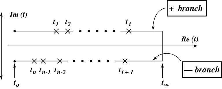
FIG. 6.: The close-time-path in the complex $t$-plane for the evolution of operator expectation values in an arbitrary initial state. Any point on the forward, positive branch $t_{0}\rightarrow t_{\infty}$ is understood at an earlier instant than any point on the backward, negative branch $t_{\infty}\rightarrow t_{0}$.

The functional $Z_{P}$ can be represented as a path integral by imposing boundary conditions in terms of complete sets of eigenstates of the gauge fields ${\cal A}_{\mu}$ at initial time $t=t_{0}$,

$${\cal A}(t_{0},\vec{x})\,|\,{\cal A}^{+}(t_{0})\,\rangle\;=\;{\cal A}^{+}(\vec{x})\,|\,{\cal A}^{+}(t_{0})\,\rangle\;,\;\;\;\;\;\;\;\;\;\;\;\;\;{\cal A}(t_{0},\vec{x})\,|\,{\cal A}^{-}(t_{0})\,\rangle\;=\;{\cal A}^{-}(\vec{x})\,|\,{\cal A}^{-}(t_{0})\,\rangle\;,$$ (B4)

and in the remote future at $t=t_{\infty}$,

$${\cal A}^{\prime}(t_{\infty},\vec{x})\,|\,{\cal A}^{\prime}(t_{\infty})\,\rangle\;=\;{\cal A}^{\prime}(\vec{x})\,|\,{\cal A}^{\prime}(t_{\infty})\,\rangle\;.$$ (B5)

Then, making use of the completeness of the eigenstates, one obtains from (B1) the following functional integral representation for $Z_{P}$,

$$Z_{P}[{\cal J}^{+},{\cal J}^{-},\hat{\rho}] = \int\,{\cal D}{\cal A}^{+}{\cal D}{\cal A}^{-}{\cal D}{\cal A}^{\prime}\;\langle\,{\cal A}^{-}(t_{0})\,|\,U^{\dagger}_{{\cal J}^{-}}(t_{0},t_{\infty})\,|\,{\cal A}(t_{\infty})\,\rangle$$ (B7)

$$\;\;\;\;\;\;\;\;\;\times\;\langle\,{\cal A}(t_{\infty})\,|\,U_{{\cal J}^{+}}(t_{\infty},t_{0})\,|\,{\cal A}^{+}(t_{0})\,\rangle\;\times\;\langle\,{\cal A}^{+}(t_{0})\,|\,\hat{\rho}\,|\,{\cal A}^{+}(t_{0})\,\rangle\;.$$

The first two amplitudes are the transition amplitudes in the presence of ${\cal J}^{+}$ and ${\cal J}^{-}$, whereas the density matrix element incorporates the initial state correlations at $t_{0}$ at the endpoints of the closed-time path $P$. Hence, one obtains the path integral representation for $Z_{P}$ in analogy to usual field theory [20, 21]

$$Z_{P}[{\cal J}^{+},{\cal J}^{-},\hat{\rho}]\;=\;\int\,{\cal D}{\cal A}^{+}{\cal D}{\cal A}^{-}\;\,\exp\left[i\left(\frac{}{}I[{\cal A}^{+}]\,+\,{\cal J}^{+}\circ{\cal A}^{+}\right)\;-\;i\left(\frac{}{}I^{\ast}[{\cal A}^{-}]\,+\,{\cal J}^{-}\circ{\cal A}^{-}\right)\right]\;{\cal M}[\hat{\rho}]\;,$$ (B8)

where

$${\cal M}(\hat{\rho})\;=\;\langle\,{\cal A}^{+}(t_{0})|\,{\hat{\rho}}\,|\,{\cal A}^{-}(t_{0})\,\rangle\;.$$ (B9)

The generalized classical action $I[{\cal A}]$ accounts for all four field orderings on the closed-time path $P$:

$$I[{\cal A}]\;\equiv\;I[{\cal A}^{+}]\,-I^{\ast}[{\cal A}^{-}]\;=\;I^{(0)}[u_{\alpha\beta}{\cal A}^{\alpha}_{\mu}{\cal A}^{\beta}_{\nu}]\;+\;I^{(1)}[g\,v_{\alpha\beta\gamma}(\partial_{\mu}{\cal A}_{\nu}^{\alpha}){\cal A}_{\mu}^{\beta}{\cal A}_{\nu}^{\gamma}]\;+\;I^{(2)}[g^{2}\,w_{\alpha\beta\gamma\delta}{\cal A}_{\mu}^{\alpha}{\cal A}_{\nu}^{\beta}{\cal A}_{\mu}^{\gamma}{\cal A}_{\nu}^{\delta}]\;,$$ (B10)

where the correspondance with the terms with the ones of (A3) is obvious (the color indices are suppressed here), and where $\alpha,\beta,\gamma,\delta=+,-$,

$$u_{\alpha\beta}\;=\;u^{\alpha\beta}\;=\;\mbox{diag}(1,-1)\;\;\;\;\;\;\;\;\;v_{\alpha\beta\gamma}\;=\;\delta_{\alpha\beta}u_{\beta\gamma}\;\;,\;\;\;\;\;\;w_{\alpha\beta\gamma\delta}\;=\;\mbox{sign}(\alpha)\,\delta_{\alpha\beta}\delta_{\beta\gamma}\delta_{\gamma\delta}\;,$$ (B11)

with the usual summation convention over repeated greek indices $\alpha,\beta,..$. Eqs. (B8)-(B10) represent the detailed version of the compact form (C1) used in Sec. 2 as the starting point, except for the Fadeev-Popov determinant and the gauge fixing constraint, which is omitted here, and which is addressed in Appendix C.

2 The density matrix and the initial state

Turning to the properties of the initial state incorporated in the functional ${\cal M}(\hat{\rho})$ with the density matrix $\hat{\rho}(t_{0})$, we denote by $t_{0}$ the initial point of time from which on the evolution of the multi-gluon state is followed, and assume that all the dynamics prior to $t_{0}$ is contained in the form of the initial state

$$|\;in\;\rangle\;\equiv\;|\;{\cal A}(t_{0})\;\rangle\;=\;\prod_{\mu,a}\,|\,{\cal A}_{\mu}^{a}(t_{0})\,\rangle\;.$$ (B12)

The initial state at $t=t_{0}$ can be constructed by expanding the gauge field operator ${\cal A}$ in the Heisenberg representation in terms of a Fock basis of non-interacting single-gluon states, the in-basis,

$${\cal A}_{\mu}^{a}(t_{0},\vec{x})\;=\;\int\frac{d^{3}k}{(2\pi)^{3}}\,\theta(k^{0})\,(2\pi)\delta(k^{2})\;\sum_{s}\left(e^{-ik\cdot x}\,\hat{c}_{\mu}^{a}(k,s)\;+\;e^{ik\cdot x}\,\hat{c}_{\mu}^{a\;\dagger}(k,s)\right)$$ (B13)

so that a particular Fock state is given by (supressing color and Lorentz indices)

$$|\,n^{(1)},n^{(2)},\ldots,n^{(\infty)}\,\rangle\;=\;\prod_{i}\,\frac{1}{\sqrt{n^{(i)}!}}\;\left(\frac{}{}\hat{c}^{\dagger}(k_{i},s_{i})\right)^{n^{(i)}}\,\;|\;0\;\rangle\;.$$ (B14)

Here $\hat{c}^{\dagger}$ ($\hat{c}$) is the creation (annihilation) operator for a single-gluon state with definite 4-momentum $k$ and spin $s$, satisfying $\hat{c}^{\dagger}\,|\,0\,\rangle=1$ ($\hat{c}\,|\,0\,\rangle=0$). and the $n^{(i)}$ are the occupation numbers of the different gluon states, $n^{(i)}\equiv\langle\,n^{(i)}|\hat{c}(k_{i},s_{i})\hat{c}^{\dagger}(k_{i},s_{i})|\,n^{(i)}\,\rangle$. Finally, $|\,0\,\rangle$ denotes the vacuum state or a ground state different from vacuum (e.g. a hadron). Thus, a general multi-gluon state $|\phi\rangle$ at time $t_{0}$ is given by a superposition of such states,

$$|\,{\cal A}(t_{0})\,\rangle\;=\;\prod_{\mu,a}\,\sum_{n^{(i)}}\,C_{\mu}^{a}(n^{(1)},n^{(2)},\ldots,n^{(\infty)})\;|\,n^{(1)},n^{(2)},\ldots,n^{(\infty)}\,\rangle\;,$$ (B15)

with real-valued coefficients $C$. Alternatively, the initial state of the system at $t_{0}$ can be characterized by the density matrix,

$$\hat{\rho}(t_{0})\;\equiv\;|\,{\cal A}(t_{0})\,\rangle\,\langle\,{\cal A}(t_{0})\,|\;\;\;\;\;\;\;\;\;\left(\,\hat{\rho}_{0}\,\right)_{ij}\;\equiv\;\langle\,n^{(i)}\,|\,\hat{\rho}(t_{0})\,|\,n^{(j)}\,\rangle\;.$$ (B16)

For instance, the case of empty vacuum corresponds to a diagonal density matrix $\hat{\rho}(t_{0})=|0\rangle\langle 0|$ with $\left(\,\hat{\rho}_{0}\,\right)_{ij}\propto\delta_{ij}$, whereas a general density matrix that describes any form of a single-particle density distribution at $t_{0}$ is

$$\hat{\rho}(t_{0})\;=\;N\;\exp\left[\sum_{s}\,\int_{\Omega}d^{3}x\int\frac{d^{3}k}{(2\pi)^{3}\,2k_{0}}\,\theta(k_{0})\,F(t_{0},\vec{x},k)\;\hat{c}_{\mu}^{a\;\dagger}(k,s)\hat{c}_{\mu}^{a}(k,s)\;\right]\;,$$ (B17)

where $\Omega$ denotes the hypersurface of the initial values and $F$ is a $c$-number function related to the single-particle phase-space density of gluons around $\vec{x}+d\vec{x}$ with four-momentum within $k^{\mu}+dk^{0}d\vec{k}$, and $N$ a normalization factor. The form (B17) describes a large class of intreresting non-equilibrium systems [19], and contains as a special case the thermal equilibrium distribution, namely when $t\rightarrow-i/T$ and $F(t_{0},\vec{x},k)\rightarrow k_{0}\,\delta(k^{2})\,T^{-1}$, so that $\hat{\rho}(T_{0})\rightarrow N\;\exp\left[-\hat{\cal H}_{YM}/T\right]$.

3 Perturbation theory and Feynman rules

The convenient feature of the CTP formalism is that it is formally completely analogous to standard quantum field theory, except for the fact that the fields have contributions from both time branches. In particular, one obtains as in usual field theory, from the path-integral representation (C17) the $n$-point Green functions $G^{(n)}(x_{1},\ldots,x_{n})$, which however now include all correlations between points on either positive and negative time branches,

$$G^{(n)}_{\alpha_{1}\alpha_{2}\ldots\,\alpha_{n}}(x_{1},\ldots,x_{n})\;\;=\;\;\left.\frac{1}{Z_{P}[0]}\;\frac{\delta}{i\,\delta{\cal K}^{(n)}}Z_{P}[{\cal K}]\right|_{{\cal K}=0}\;\;,\;\;\;\;\;\;\;\;\;\;\;\;\alpha_{i}\;=\pm\;,$$ (B18)

depending on whether the space-time points $x_{i}$ lie on the $+$ or $-$ time branch. One can then construct a perturbative expansion of the non-equilibrium Green functions in terms of modified Feynman rules (as compared to standard field theory) [18, 19, 22].

  (i)

All local 1-point functions $G^{(1)}_{\alpha}(x)$, such as the gauge-field or the color current, are ‘vectors’ with 2 components,

$${\cal A}(x)\;\equiv\;\left(\begin{array}[]{c}{\cal A}^{+}\\ {\cal A}^{-}\end{array}\right)\;\;\;\;\;\;\;\;\;\;\;\;\;\;\;\;{\cal J}(x)\;\equiv\;\left(\begin{array}[]{c}{\cal J}^{+}\\ {\cal J}^{-}\end{array}\right)$$ (B19)

Similarly, all 2-point functions $G^{(2)}_{\alpha\beta}(x,y)$, such as the as the gluon propagator $i\Delta_{\mu\nu}$ and the polarization tensor $\Pi_{\mu\nu}$, are 2$\times$2 matrices with components,

$$\Delta(x_{1},x_{2})\;\equiv\;\left(\begin{array}[]{cc}\Delta^{++}&\;\Delta^{+-}\\ \Delta^{-+}&\;\Delta^{--}\end{array}\right)\;\;\;\;\;\;\;\;\;\;\;\;\;\;\;\;\Pi(x_{1},x_{2})\;\equiv\;\left(\begin{array}[]{cc}\Pi^{++}&\;\Pi^{+-}\\ \Pi^{-+}&\;\Pi^{--}\end{array}\right)\;.$$ (B20)

Explicitely, the components of the propagator are

$$\Delta_{\mu\nu}^{F}(x,y)\; \equiv \Delta_{\mu\nu}^{++}(x,y)\;=\;-i\,\langle\;T\,{\cal A}_{\mu}^{+}(x)\,{\cal A}_{\nu}^{+}(y)\;\rangle\;\;\;\;\;\;\;\;\;\;\;\;\Delta_{\mu\nu}^{<}(x,y)\;\;\equiv\;\Delta_{\mu\nu}^{+-}(x,y)\;=\;-i\,\langle\;{\cal A}_{\nu}^{+}(y)\,{\cal A}_{\mu}^{-}(x)\;\rangle$$ (B21)

$$\Delta_{\mu\nu}^{>}(x,y)\; \equiv \Delta_{\mu\nu}^{-+}(x,y)\;=\;-i\,\langle\;{\cal A}_{\mu}^{-}(x)\,{\cal A}_{\nu}^{+}(y)\;\rangle\;\;\;\;\;\;\;\;\;\;\;\;\;\;\Delta_{\mu\nu}^{\overline{F}}(x,y)\;\;\equiv\;\Delta_{\mu\nu}^{--}(x,y)\;=\;-i\,\langle\;\overline{T}\,{\cal A}_{\mu}^{-}(x)\,{\cal A}_{\nu}^{-}(y)\;\rangle\;,$$ (B22)

where $\Delta^{F}$ is the usual time-ordered Feynman propagator, $\Delta^{\overline{F}}$ is the corresponding anti-time-ordered propagator, and $\Delta^{>}$ ($\Delta^{<}$) is the unordered correlation function for $x_{0}>y_{0}$ ($x_{0}<y_{0}$). In compact notation,

$$\Delta_{\mu\nu}(x,y)\;=\;-i\,\langle\,T_{P}{\cal A}(x){\cal A}(y)(y)\,\rangle\;,$$ (B23)

where the generalized time-ordering operator $T_{P}$ is defined as

$$T_{P}\,A(x)B(y)\;:=\;\theta_{P}(x_{0},y_{0})\,A(x)B(y)\;+\;\theta_{P}(y_{0},x_{0})\,B(y)A(x)\;,$$ (B24)

with the $\theta_{P}$-function defined as

$$\theta_{P}(x_{0},y_{0})\;=\;\left\{\begin{array}[]{ll}1&\;\;\mbox{if $x_{0}$ {\it succeeds} $y_{0}$ on the contour $P$}\\ 0&\;\;\mbox{if $x_{0}$ {\it precedes} $y_{0}$ on the contour $P$}\end{array}\right.\;.$$ (B25)

Higher order products $A(x)B(y)C(z)\ldots$ are ordered analogously. Finally, the generalized $\delta_{P}$-function on the closed-time path $P$ is defined as:

$$\delta^{4}_{P}(x,y)\;\,:=\;\,\left\{\begin{array}[]{ll}+\delta^{4}(x-y)&\;\;\mbox{if}\;x_{0}\;\mbox{and}\;y_{0}\;\mbox{from positive branch}\\ -\delta^{4}(x-y)&\;\;\mbox{if}\;x_{0}\;\mbox{and}\;y_{0}\;\mbox{from negative branch}\\ 0&\;\;\mbox{otherwise}\end{array}\right.\;.$$ (B26)

  (ii)

The number of elementary vertices is doubled, because each propagator line of a Feynman diagram can be either of the four components of the Green functions. The interaction vertices in which all the fields are on the $+$ branch are the usual ones, while the vertices in which the fields are on the $-$ branch have the opposite sign. On the other hand, combinatoric factors, rules for loop integrals, etc., remain the same as in usual field theory. Specifically, the 3-gluon and 4-gluon vertices,

$$G^{(3)}_{\alpha\beta\gamma}(x_{1},x_{2},x_{3}) \equiv \int_{P}d^{4}x\,G^{(2)}_{\alpha^{\prime}\alpha}(x_{1},x)G^{(2)}_{\beta^{\prime}\beta}(x_{2},x)G^{(2)}_{\gamma^{\prime}\gamma}(x_{3},x)\;\;\Gamma^{(3)}_{\alpha^{\prime}\beta^{\prime}\gamma^{\prime}}(x)$$ (B27)

$$G^{(4)}_{\alpha\beta\gamma\delta}(x_{1},x_{2},x_{3},x_{4}) \equiv \int_{P}d^{4}x\,G^{(2)}_{\alpha^{\prime}\alpha}(x_{1},x)G^{(2)}_{\beta^{\prime}\beta}(x_{2},x)G^{(2)}_{\gamma^{\prime}\gamma}(x_{3},x)G^{(2)}_{\delta^{\prime}\delta}(x_{4},x)\;\;\Gamma^{(4)}_{\alpha^{\prime}\beta^{\prime}\gamma^{\prime}\delta^{\prime}}(x)\;,$$ (B28)

with $\Gamma^{(3)}(x)$ and $\Gamma^{(4)}(x)$ denoting the elementary, amputated vertices (with the external legs removed), have, for fixed $\alpha,\beta,\gamma,\delta$ two components. For instance, as in Fig. 7, for the external points on the $+$-branch,

$$\mbox{for $\alpha=\beta=\gamma=\,+$}: \;\;\;\;\;\;\Gamma^{(3)}_{\alpha^{\prime}\beta^{\prime}\gamma^{\prime}}(x)\;\;=\;\;\left(\Gamma^{(3)}_{+++},\;-\,\Gamma^{(3)}_{---}\right)$$ (B29)

$$\mbox{for $\alpha=\beta=\gamma=\delta=\,+$}: \;\;\;\;\Gamma^{(4)}_{\alpha^{\prime}\beta^{\prime}\gamma^{\prime}\delta^{\prime}}(x)\;=\;\left(\Gamma^{(4)}_{++++},-\,\Gamma^{(4)}_{----}\right)$$ (B30)

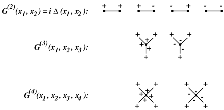
FIG. 7.: Example for the appearance of additional contributions to the $n$-point functions $G^{(n)}$ for the propagator $G^{(2)}$, the 3-vertex $G^{(3)}$, and the 4-vertex $G^{(4)}$ In usual quantum field theory referring to free space or ‘vacuum’, only the $+$-graphs are non-zero. In the CTP formalism, accounting for the presence of surrounding matter or ‘medium’, new diagrams arise that correspond to statistical correlations between the field living on the $+$ and $-$ time branches of Fig. 6.

C The in-in amplitude $Z_{P}$ for QCD in non-covariant gauges

For the case of QCD, path-integral representation of the in-in amplitude $Z_{P}$ is obtained along the lines of Appendix B1, except that one has to extend the generic formula (B8) to account for eliminating the spurious gauge degrees of freedom by the usual Fadeev-Popov procedure [45]. The gauge theory version of (B8) for the class of non-covariant gauges (2) reads therefore:

$$Z_{P}[{\cal J},\hat{\rho}]\;=\;{\cal N}\;\int\,{\cal D}{\cal A}\;\mbox{det}{\cal F}\;\delta\left(f[{\cal A}]\right)\;\,\exp\left\{i\left(\frac{}{}I\left[{\cal A},{\cal J}\right]\right)\right\}\;\;{\cal M}(\hat{\rho})\;,$$ (C1)

where ${\cal A}=({\cal A}^{+},{\cal A}^{-})$ and ${\cal J}=({\cal J}^{+},{\cal J}^{-})$ have two components, living on the $+$ and $-$ time branches of Fig. 2. Physical expectation values are defined as functional averages over $T_{P}$-ordered products of $n$ field operators ($n\geq 1$), weighted by $Z_{P}$,

$$\langle\;{\cal O}_{1}(x_{1})\ldots{\cal O}_{n}(x_{n})\;\rangle_{P}\;\equiv\;\frac{1}{Z_{P}[0,\hat{\rho}]}\;\int\,{\cal D}{\cal A}\;\mbox{det}{\cal F}\;\delta\left(f[{\cal A}]\right)\exp\left\{i\left(\frac{}{}I\left[{\cal A},{\cal J}\right]\right)\right\}\,\,{\cal M}(\hat{\rho})\;\;\;T_{P}\left[{\cal O}_{1}(x_{1})\ldots{\cal O}_{n}(x_{n})\right]\;.$$ (C2)

The structure of the functional $Z_{P}$ in (C1) and (C2) is the following:

  (i)

The functional integral (with normalization ${\cal N}$) is over all gauge field configurations with measure ${\cal D}{\cal A}\equiv\prod_{\mu,a}{\cal D}{\cal A}_{\mu}^{a}$, subject to the condition of gauge fixing, here for the class of non-covariant gauges defined by

$$f^{a}[{\cal A}]\;:=\;n\cdot{\cal A}^{a}(x)\;-\;B^{a}(x)\;\;\;\;\;\;\;\;\;\;\;\Longrightarrow\;\;\;\;\;\;\;\;\;\;\langle\;n^{\mu}\,{\cal A}_{\mu}^{a}(x)\;\rangle\;=\;0\;,\;\;\;\;\;\;\;\;\;\;\;\;\;n^{\mu}\,\equiv\,\frac{n^{\mu}}{\sqrt{|n^{2}|}}\;,$$ (C3)

where $n^{\mu}$ is a constant 4-vector, being either space-like ($n^{2}<0$), time-like ($n^{2}>0$), or light-like ($n^{2}=0$). With this choice of gauge class the local gauge constraint on the fields ${\cal A}^{a}_{\mu}(x)$ in the path-integral (C1) becomes,

$$\mbox{det}{\cal F}\;\delta\left(n\cdot{\cal A}^{a}-B^{a}\right)\;=\;\mbox{const}\,\times\,\exp\left\{i\,I_{GF}\left[n\cdot{\cal A}\right]\right\}$$ (C4)

$$I_{GF}\left[n\cdot{\cal A}\right]\;=\;-\frac{1}{2\alpha}\int_{P}d^{4}x\,\left[n\cdot{\cal A}^{a}(x)\right]^{2}\;,$$ (C5)

where $\mbox{det}{\cal F}$ is the Fadeev-Popov determinant (which in the case of the non-covariant gauges turns out to be a constant factor, c.f. Appendix C), and where $\delta(n\cdot{\cal A})\equiv\prod_{a}\delta(n\cdot{\cal A}^{a})$. The right side translates this constraint into a the gauge fixing functional $I_{GF}$. The particular choice of the vector $n^{\mu}$ and of the real-valued parameter $\alpha$ is dictated by the physics or computational convenience, and distinguishes further within the class of non-covariant gauges [27, 28]:

$$\mbox{homogenous axial gauge}:\; \;\;\;\;\;n^{2}\;<\;0\;\;\;\;\;\;\alpha\;=\;0$$ (C6)

$$\mbox{inhomogenous axial gauge}:\; \;\;\;\;\;n^{2}\;<\;0\;\;\;\;\;\;\alpha\;=\;1$$ (C7)

$$\mbox{temporal axial gauge}:\; \;\;\;\;\;n^{2}\;>\;0\;\;\;\;\;\;\alpha\;=\;0$$ (C8)

$$\mbox{lightcone gauge}:\; \;\;\;\;\;n^{2}\;=\;0\;\;\;\;\;\;\alpha\;=\;0\;.$$ (C9)

  (ii)

The exponential $I$ is the effective classical action with respect to both the $+$ and the $-$ time contour, $I\left[{\cal A},{\cal J}\right]\equiv I\left[{\cal A}^{+},{\cal J}^{+}\right]\;-\;I^{\ast}\left[{\cal A}^{-},{\cal J}^{-}\right]$, including the usual Yang-Mills action $I_{YM}=\int d^{4}x{\cal L}_{YM}$, plus the source ${\cal J}$ coupled to the gauge field ${\cal A}$:

$$I\left[{\cal A},{\cal J}\right] = -\frac{1}{4}\int_{P}d^{4}x\,{\cal F}_{\mu\nu}^{a}(x){\cal F}^{\mu\nu,\,a}(x)\;+\;\int_{P}d^{4}x\,{\cal J}_{\mu}^{a}(x){\cal A}^{\mu,\,a}(x)$$ (C10)

$$\equiv \;\;\;\;\;\;\;\;I_{YM}\left[{\cal A}\right]\;\;\;+\;\;\;{\cal J}\circ{\cal A}\;.$$ (C12)

  (iii)

The form of the initial state at $t=t_{0}$ as described by the density matrix $\hat{\rho}$ (an example is given in Appendix B2, eq. (B16)) is embodied in the function ${\cal M}(\hat{\rho})$ which is the density-matrix element of the gauge fields at initial time $t_{0}$,

$${\cal M}(\hat{\rho})\;=\;\langle\,{\cal A}^{+}(t_{0})|\,{\hat{\rho}}\,|\,{\cal A}^{-}(t_{0})\,\rangle\;\equiv\;\,\exp\left(i\;{\cal K}[{\cal A}]\right)\;,$$ (C13)

where ${\cal A}^{\pm}$ refers to the $+$ and $-$ time branch at $t_{0}$, respectively (c.f. Fig. 2). The functional ${\cal K}$ may be expanded in a series of non-local kernels corresponding to multi-point correlations concentrated at $t=t_{0}$,

$${\cal K}[{\cal A}] = {\cal K}^{(0)}\;+\;\int_{P}d^{4}x\;{\cal K}^{(1)\;a}_{\;\;\;\,\mu}(x)\;{\cal A}^{\mu,\,a}(x)\;+\;\frac{1}{2}\int_{P}d^{4}xd^{4}y\;{\cal K}^{(2)\;ab}_{\;\;\;\,\mu\nu}(x,y)\;{\cal A}^{\mu,\,a}(x)\,{\cal A}^{\nu,\,b}(y)\,\ldots$$ (C15)

$$\;\;\;\;\;\;\;\;\;\;\;\;\;\;\equiv\;\sum_{n=0}^{\infty}\;\,\frac{1}{n!}\;{\cal K}^{(n)}\circ\left(\frac{}{}{\cal A}(1)\,{\cal A}(2)\,\ldots\,{\cal A}(n)\right)\;.$$

Clearly, the sequence of kernels ${\cal K}^{(n)}$ contains as much information as the original density matrix. In the special case that $\hat{\rho}$ is diagonal, the kernels ${\cal K}^{(n)}=0$ for all $n$, and the usual ‘vacuum field theory’ is recovered.

The path-integral representation (C1) can be rewritten in a more convenient form: First, the gauge-fixing functional $I_{GF}[n\cdot{\cal A}]$ is implemented, using (C5). Second, the series representation (C15) is inserted into the initial state functional ${\cal M}(\hat{\rho})$. Third, ${\cal K}^{(0)}$ is absorbed in the overall normalization ${\cal N}$ of $Z_{P}$ (henceforth set to unity), and the external source ${\cal J}$ in the 1-point kernel ${\cal K}^{(1)}$:

$${\cal K}^{(0)}\;:=\;i\,\ln{\cal N}\;,\;\;\;\;\;\;\;\;\;\;\;\;\;\;{\cal K}^{(1)}\;:=\;{\cal K}^{(1)}\;+\;{\cal J}\;.$$ (C16)

Then (C1) becomes,

$$Z_{P}[{\cal J},\hat{\rho}]\;\;\Longrightarrow\;\;Z_{P}[{\cal K}]\;=\;\int\,{\cal D}{\cal A}\;\exp\left\{i\left(\frac{}{}I\left[{\cal A},{\cal K}\right]\right)\right\}\;,$$ (C17)

where, instead of (C12),

$$I\left[{\cal A},{\cal K}\right]\;\equiv\;I_{YM}\left[{\cal A}\right]\;+\;I_{GF}\left[n\cdot{\cal A}\right]\;+\;{\cal K}^{(1)}\circ{\cal A}\;+\;\frac{1}{2}\,{\cal K}^{(2)}\circ\left({\cal A}\,{\cal A}\right)\;+\;\frac{1}{6}\,{\cal K}^{(3)}\circ\left({\cal A}\,{\cal A}\,{\cal A}\right)\;+\;\ldots\;.$$ (C18)

The objects of physical relevance are the $n$-point Green functions $G^{(n)}$, defined as the coefficients in a functional expansion of $Z_{P}$,

$$Z_{P}[{\cal K}]\;=\;Z_{P}[0]\;\,\sum_{n=1}^{\infty}\,\frac{i^{n}}{n!}\int\prod_{i=1}^{n}d^{4}x_{i}\;G^{(n)}(x_{1},\ldots,x_{n})\,\;{\cal K}^{(n)}(x_{1},\ldots,x_{n})\;,$$ (C19)

that is, the $G^{(n)}$ are functional averages in the sense of (C2),

$$G_{\;\;\;\mu_{1}\ldots\mu_{n}}^{(n)\;a_{1}\ldots a_{n}}(x_{1},\ldots,x_{n})\;\;\equiv\;\;\langle\;{\cal A}_{\mu_{1}}^{a_{1}}(x_{1})\ldots{\cal A}_{\mu_{n}}^{a_{n}}(x_{n})\;\rangle_{P}\;\;=\;\;\left.\frac{1}{Z_{P}[0]}\;\frac{\delta}{i\,\delta{\cal K}^{(n)}}Z_{P}[{\cal K}]\right|_{{\cal K}=0}\;.$$ (C20)

The practical evaluation of $Z_{P}$ amounts therefore to calculating the $G^{(n)}$ in the expansion (C19) up to the order of desired accuracy. For instance, the 1-, 2-, and 3-point Green functions according to (C20) are

$$G_{\;\;\;\;\mu}^{(1)\;a}(x) = \langle\;{\cal A}_{\mu}^{a}(x)\;\rangle_{P}$$ (C21)

$$G_{\;\;\;\;\mu\nu}^{(2)\;ab}(x,y) = \langle\;{\cal A}_{\mu}^{a}(x){\cal A}_{\nu}^{b}(y)\;\rangle_{P}\;=\;\frac{\delta}{i\,\delta{\cal K}_{\;\;\;\mu}^{(1)\;a}(x)}\,\langle\;{\cal A}_{\nu}^{b}(y)\;\rangle_{P}\;+\;\langle\;{\cal A}_{\mu}^{a}(x)\;\rangle_{P}\langle\;{\cal A}_{\nu}^{b}(y)\;\rangle_{P}$$ (C22)

$$G_{\;\;\;\;\mu\nu\lambda}^{(3)\;abc}(x,y,z) = \langle\;{\cal A}_{\mu}^{a}(x){\cal A}_{\nu}^{b}(y){\cal A}_{\lambda}^{c}(z)\;\rangle_{P}\;=\;\frac{1}{2}\left(\frac{\delta}{i\,\delta{\cal K}_{\;\;\;\mu\nu}^{(2)\;ab}(x,y)}\;+\;\frac{\delta}{i\,\delta{\cal K}_{\;\;\;\mu}^{(1)\;a}(x)}\frac{\delta}{i\,\delta{\cal K}_{\;\;\;\nu}^{(1)\;b}(y)}\right)\,\langle\;{\cal A}_{\lambda}^{c}(z)\;\rangle_{P}$$ (C24)

$$\;\;\;\;\;\;\;\;\;+\;\frac{\delta}{i\,\delta{\cal K}_{\;\;\;\mu}^{(1)\;a}(x)}\left(\frac{}{}\langle\;{\cal A}_{\nu}^{b}(y)\;\rangle_{P}\langle\;{\cal A}_{\lambda}^{c}(z)\;\rangle_{P}\right)\;+\;\langle\;{\cal A}_{\mu}^{a}(x)\;\rangle_{P}\langle\;{\cal A}_{\nu}^{b}(y)\;\rangle_{P}\langle\;{\cal A}_{\lambda}^{c}(z)\;\rangle_{P}\;.$$

Higher order Green functions are generated similarly from ((C20).

D Non-covariant gauges and the absence of ghosts

In this appendix the standard procedure of gauge field quantization is applied to the class of non-covariant gauges (C9), and it is shown that ghost degrees of freedom are indeed absent, reducing the general non-linear dynamics in of QCD essentially to a linear QED type dynamics. For an excellent review and bibliography, see Ref. [27]. Recall that under local gauge transformations

$$g[\theta^{a}]\;\equiv\;\exp\left(-i\,\theta^{a}(x)\,T^{a}\right)\;,$$ (D1)

the gauge fields transform as

$${\cal A}_{\mu}^{a}\;\longrightarrow\;{\cal A}_{\mu}^{(\theta)\;a}\;=\;g[\theta^{a}]\;{\cal A}_{\mu}^{a}\;g^{-1}[\theta^{a}]\;,$$ (D2)

implying that ${\cal F}_{\mu\nu}^{a}{\cal F}_{\mu\nu}^{a}\;=\;{\cal F}_{\mu\nu}^{(\theta)\;a}{\cal F}_{\mu\nu}^{(\theta)\;a}$, that is the gauge invariance of the Yang-Mills action $I_{YM}[{\cal A}]$. However, the source term ${\cal J}\circ{\cal A}$ in the generating functional $Z_{P}$ of (C1) is not gauge invariant under the transformations (D1). Consequently, the naive functional

$$Z_{P}^{(naive)}\;=\;\int\,{\cal D}{\cal A}\;\exp\left\{i\left(\frac{}{}I_{YM}\left[{\cal A}\right]+{\cal J}\circ{\cal A}\right)\right\}\,\times\,{\cal M}(\hat{\rho})$$ (D3)

is also not a gauge invariant quantity. As is well known, this can be remedied by applying the formal Fadeev-Popov [45] procedure and integrate in the path-integral $Z_{P}$ over all possible gauge transformations $g(\theta^{a})$ subject to the linear subsidiary condition

$$\phi^{a}[{\cal A}_{\mu}^{(\theta)}]\;\equiv\;n^{\mu}\,{\cal A}_{\mu}^{(\theta)\;a}(x)\;-\;\beta^{a}(x)\;\stackrel{{\scriptstyle!}}{{=}}\;0$$ (D4)

with normalized space-like vector $n^{\mu}$ and $\beta^{a}(x)$ an arbitrary weight function. The Fadeev-Popov trick to implement the constraint (D4) in the non-invariant functional $Z_{P}^{(naive)}$ by multiplying with

$$1\;\,=\;\,\int{\cal D}\theta\;\prod_{a}\delta\left(\phi^{a}[{\cal A}_{\mu}^{(\theta)}]\right)\;\mbox{det}{\cal F}\;,$$ (D5)

where the determinant is the Jacobian for the change of variables $\phi^{a}\rightarrow\theta^{a}$,

$$\left(\frac{}{}\mbox{det}{\cal F}\right)^{ab}\;=\;\mbox{det}\left(\frac{\delta\phi^{a}[{\cal A}_{\mu}^{(\theta)}]}{\delta\theta^{b}}\right)_{\phi^{a}[{\cal A}_{\mu}^{(\theta)}]=0}\;=\;\left\{\int{\cal D}\theta\;\prod_{a}\delta\left(\phi^{a}[{\cal A}_{\mu}^{(\theta)}]\right)\right\}^{-1}\;.$$ (D6)

Following this procedure one arrives at

$$Z_{P}^{(naive)}\;\longrightarrow\;Z_{P}\;=\;\int\,{\cal D}{\cal A}\;\mbox{det}{\cal F}\;\prod_{a}\delta\left(\phi^{a}[{\cal A}_{\mu}]\right)\;\exp\left\{i\left(\frac{}{}I_{YM}\left[{\cal A}\right]+{\cal J}\circ{\cal A}\right)\right\}\,\times\,{\cal M}(\hat{\rho})\;,$$ (D7)

which is now a gauge invariant expression due to the proper account of the subsidiary condition (D4) that guarantees the correct transformation properties of the gauge fields in the presence of the sources ${\cal J}$.

To obtain the final form of $Z_{P}$ as quoted in (C1), one integrates functionally over the arbitrary funtions $\beta^{a}(x)$ introduced in (D4), by choosing, e.g., a Gaussian weight functional

$$w[\beta^{a}]\;=\;\exp\left\{-\frac{i}{2\alpha}\,\int_{P}d^{4}x\,\left[\beta^{a}(x)\right]^{2}\right\}\;,$$ (D8)

with the real valued parameter $0\leq\alpha\leq 1$, upon which the Fadeev-Popov determinant $\mbox{det}{\cal F}$ can be rewritten in a more suitable way:

$$\mbox{det}{\cal F}\;=\;\int{\cal D}\beta\;\prod_{a}\;\exp\left\{-\frac{i}{2\alpha}\,\int_{P}d^{4}x\,\left[\beta^{a}(x)\right]^{2}\right\}\;\delta\left(n^{\mu}\,{\cal A}_{\mu}^{(\theta)\;a}(x)\;-\;\beta^{a}(x)\right)\;.$$ (D9)

In order to calculate the determinant, it is sufficient to integrate over $\theta^{a}$ in a small vicinity where the argument of the $\delta$-function passes through zero at given ${\cal A}^{(\theta)\;a}$ and $\beta^{a}$. For infinitesimal gauge transformations

$$g[\theta^{a}]\;\longrightarrow\;\delta g[\theta^{a}]\;=\;1\;-\;i\theta^{a}(x)\,T^{a}\;,$$ (D10)

the gauge fields transform as

$${\cal A}_{\mu}^{a}\;\longrightarrow\;{\cal A}_{\mu}^{a}\;+\;\delta{\cal A}_{\mu}^{a}\;\;,\;\;\;\;\;\;\;\;\;\;\;\;\;\;\delta{\cal A}_{\mu}^{a}\;=\;f^{abc}\theta^{b}{\cal A}_{\mu}^{c}\;-\;\frac{1}{g}\,\partial_{\mu}^{x}\theta^{a}\;,$$ (D11)

so that one obtains

$$\;\delta\left(n^{\mu}\,{\cal A}_{\mu}^{(\theta)\;a}(x)\;-\;\beta^{a}(x)\right) = \;\delta\left(n^{\mu}\,{\cal A}_{\mu}^{(\theta)\;a}(x)\;+\;f^{abc}\theta^{b}\,n^{\mu}{\cal A}_{\mu}^{(\theta)\;c}\;-\;\frac{1}{g}\,n^{\mu}\partial_{\mu}^{x}\,\theta^{a}\;-\;\beta^{a}\right)$$ (D12)

$$= \;\delta\left(f^{abc}\theta^{b}\,\beta^{c}\;-\;\frac{1}{g}\,n^{\mu}\partial_{\mu}^{x}\,\theta^{a}\right)\;,$$ (D13)

because $n^{\mu}{\cal A}_{\mu}^{(\theta)\;a}=\beta^{a}$. This latter expression is evidently independent of ${\cal A}_{\mu}^{a}$. Therefore, when substituted into (D9), $\mbox{det}{\cal F}$ is also explicitely independent of the gauge fields, and hence can be pulled out of the path-integral $Z_{P}$ and absorbed in an (irrelevant) normalization, which may be set equal to unity. The final result is then:

$$Z_{P}[{\cal J},\hat{\rho}]\;=\;\int\,{\cal D}{\cal A}\;\;\exp\left\{i\left(\frac{}{}I_{YM}\left[{\cal A}\right]\;+\;I_{GF}\left[n\cdot{\cal A}\right]\;+\;{\cal J}\circ{\cal A}\right)\right\}\,\times\,{\cal M}(\hat{\rho})\;,$$ (D14)

where, from (D9),

$$I_{GF}\left[n\cdot{\cal A}\right]\;\equiv\;\exp\left\{-\frac{i}{2\alpha}\,\int_{P}d^{4}x\,\left[n\cdot{\cal A}^{a}(x)\right]^{2}\right\}\;.$$ (D15)

In conclusion: the property of gauge field independence of the Fadeev-Popov determinant proves that there are indeed no ghost fields coupling to the gluon fields, hence the formulation is ghost-free!

E The truncated effective action $\Gamma_{P}\left[\overline{A},\widehat{\Delta}\right]$

The generating functional for the connected Green functions, denoted by ${\cal G}^{(n)}$, is defined as usual:

$$W_{P}\left[{\cal K}\right]\;\;=\;\;-i\,\ln\,Z_{P}\left[{\cal K}\right]\;.$$ (E1)

From $W_{P}$ one obtains the connected Green functions ${\cal G}^{(n)}$ by functional differentiation analogous to (C20), in terms of mixed products of $a_{\mu}$ and $A_{\mu}$ fields

$$(-i)\,{\cal G}_{\;\;\;\;\mu_{1}\ldots\mu_{n}}^{(n)\;a_{1}\ldots a_{n}}(x_{1},\ldots,x_{n})\;\equiv\;\left.\frac{\delta}{i\,\delta{\cal K}^{(n)}}W_{P}[{\cal K}]\right|_{{\cal K}=0}\;\;=\;\;\langle\;a_{\mu_{1}}^{a_{1}}(x_{1})\ldots a_{\mu_{k}}^{a_{k}}(x_{k})\,A_{\mu_{k+1}}^{a_{k+1}}(x_{k+1})\ldots A_{\mu_{n}}^{a_{n}}(x_{n})\;\rangle_{P}^{(c)}\;,$$ (E2)

where the superscript $(c)$ indicates the ‘connected parts’. It follows then that

$$\frac{\delta W_{P}}{\delta{\cal K}^{(1)\;\mu,a}(x)} = \;\;\;\;{\cal G}_{\;\;\;\;\mu}^{(1)\;a}(x)$$ (E3)

$$\frac{\delta W_{P}}{\delta{\cal K}^{(2)\;\mu\nu,ab}(x,y)} = \frac{1}{2}\,\left({\cal G}_{\;\;\;\;\mu\nu}^{(2)\;ab}(x,y)\;+\;{\cal G}_{\;\;\;\mu}^{(1)\;a}(x){\cal G}_{\;\;\;\nu}^{(1)\;b}(y)\right)$$ (E4)

$$\frac{\delta W_{P}}{\delta{\cal K}^{(3)\;\mu\nu\lambda,abc}(x,y,z)} = \frac{1}{6}\,\left({\cal G}_{\;\;\;\;\mu\nu\lambda}^{(3)\;abc}(x,y,z)\;+\;3\;{\cal G}_{\;\;\;\;\mu\nu}^{(2)\;ab}(x,y)\,{\cal G}_{\;\;\;\;\lambda}^{(1)\;c}(z)\;+\;{\cal G}_{\;\;\;\mu}^{(1)\;a}(x){\cal G}_{\;\;\;\nu}^{(1)\;b}(y){\cal G}_{\;\;\;\lambda}^{(1)\;c}(z)\right)\;,$$ (E5)

where, for example,

$${\cal G}_{\;\;\;\;\mu}^{(1)\;a}(x) = \langle\;A_{\mu}^{a}(x)\;\ \rangle_{P}^{(c)}\;+\;\langle\;a_{\mu}^{a}(x)\rangle_{P}^{(c)}$$ (E6)

$${\cal G}_{\;\;\;\;\mu\nu}^{(2)\;ab}(x,y) = \langle\;A_{\mu}^{a}(x)A_{\nu}^{b}(y)\;\rangle_{P}^{(c)}\;+\;\langle\;a_{\mu}^{a}(x)a_{\nu}^{b}(y)\;\rangle_{P}^{(c)}$$ (E7)

$${\cal G}_{\;\;\;\;\mu\nu\lambda}^{(3)\;abc}(x,y,z) = \langle\;A_{\mu}^{a}(x)A_{\nu}^{b}(y)A_{\lambda}^{c}(z)\;\rangle_{P}^{(c)}\;+\;\langle\;a_{\mu}^{a}(x)a_{\nu}^{b}(y)a_{\lambda}^{c}(z)\;\rangle_{P}^{(c)}\;,$$ (E8)

and similarly expressions higher order Green functions which involve 4, 5 … space-time points.

$W_{P}$ of (E1) involves the sources ${\cal K}$ that do not have any immediate physical interpretation, it is more convenient to work with the corresponding effective action $\Gamma_{P}$, the generating functional for the proper vertex functions, which determines the equations of motion for the physically relevant Green functions. The effective action $\Gamma_{P}$ is defined as the multiple Legendre transform, and is obtained by eliminating the source variables ${\cal K}$ in favor of the connected Green functions ${\cal G}$:

$$\Gamma_{P}\left[{\cal G}\right] = W_{P}\left[{\cal K}\right]\;-\;{\cal K}^{(1)}\circ{\cal G}^{(1)}\;-\;\frac{1}{2}{\cal K}^{(2)}\circ\left({\cal G}^{(2)}+{\cal G}^{(1)}{\cal G}^{(1)}\right)$$ (E10)

$$\;\;\;\;\;\;\;\;\;\;\;\;\;\;\;\;-\;\frac{1}{6}{\cal K}^{(3)}\circ\left({\cal G}^{(3)}+3\,{\cal G}^{(2)}{\cal G}^{(1)}+{\cal G}^{(1)}{\cal G}^{(1)}{\cal G}^{(1)}\right)\;-\;\ldots\;.$$

So far no approximations have been made. The variation of $\Gamma_{P}$ with respect to the Green functions ${\cal G}^{(n)}$ would yield an infinite set of coupled equations, the analogue of the BBGKY hierarchy [14]:

$$\frac{\delta\Gamma_{P}}{{\cal G}^{(1)}} = -{\cal K}^{(1)}\;-\;{\cal K}^{(2)}\circ{\cal G}^{(1)}\;-\;-\frac{1}{2}{\cal K}^{(3)}\circ\left({\cal G}^{(2)}+{\cal G}^{(1)}{\cal G}^{(1)}\right)\;-\;\ldots$$ (E11)

$$\frac{\delta\Gamma_{P}}{{\cal G}^{(2)}} = -\frac{1}{2}{\cal K}^{(2)}-\frac{1}{2}{\cal K}^{(3)}\circ{\cal G}^{(1)}\;-\;\ldots$$ (E12)

$$\frac{\delta\Gamma_{P}}{{\cal G}^{(3)}} = -\frac{1}{6}{\cal K}^{(3)}\;-\;\ldots\;,\;\;\;\;\;\;\;\;\;\;\mbox{etc.}$$ (E13)

At this point approximation 1 and 2 of Section II A are invoked. It is assumed that the initial state is a (dilute) ensemble of hard gluons of very small spatial extent $\ll\lambda$, corresponding to transverse momenta $k_{\perp}^{2}\gg\mu^{2}$. By definition of $\lambda$, or $\mu$, the short-range character of these quantum fluctuations implies that the expectation value $\langle a_{\mu}\rangle$ vanishes at all times. However, the long-range correlations of the eventually populated soft modes with very small momenta $k_{\perp}^{2}\ll\mu^{2}$ may lead to a collective mean field with non-vanishing $\langle A\rangle$. Accordingly, the following condition is imposed on the expectation values of the fields:

$$\langle\;A_{\mu}^{a}(x)\;\rangle\;\left\{\begin{array}[]{ll}\;=\;0\;\;\;\mbox{for}\;t\,\leq\,t_{0}\\ \;\geq\;0\;\;\;\mbox{for}\;t\,>\,t_{0}\end{array}\right.\;\;\;\;\;\;\;\;\;\;\;\;\;\;\;\;\;\;\;\;\langle\;a_{\mu}^{a}(x)\;\rangle\;\stackrel{{\scriptstyle!}}{{=}}\;0\;\;\;\mbox{for all}\;t\;.$$ (E14)

Furthermore, the quantum fluctuations of the soft field are ignored, assuming any multi-point correlations of soft fields to be small,

$$\langle\;A_{\mu_{1}}^{a_{1}}(x_{1})\;\ldots A_{\mu_{n}}^{a_{n}}(x_{n})\;\rangle\ll\;\langle\;A_{\mu_{1}}^{a_{1}}(x_{1})\;\rangle\;\ldots\;\langle\;A_{\mu_{1}}^{a_{n}}(x_{n})\;\rangle\;\;\;\;\;\;\mbox{for all $n\geq 2$}\;,$$ (E15)

i.e., $A_{\mu}$ is treated as a non-propagating and non-fluctuating, classical field. Hence, the set of Green functions (E8) reduces to

$${\cal G}_{\;\;\;\;\mu}^{(1)\;a}(x)\;=\;\langle\;A_{\mu}^{a}(x)\;\rangle_{P}^{(c)}\;\;\equiv\;\;\overline{A}_{\mu}^{a}(x)\;\;\;\;\;\;\;\;\;{\cal G}_{\;\;\;\;\mu\nu}^{(2)\;ab}(x,y)\;=\;\langle\;a_{\mu}^{a}(x)a_{\nu}^{b}(y)\;\rangle_{P}^{(c)}\;\;\equiv\;\;i\widehat{\Delta}_{\mu\nu}^{ab}(x,y)\;.$$ (E16)

These relations define the soft, classical mean field $\overline{A}$, and the hard quantum propagators $\widehat{\Delta}$.

Now the hierarchy is truncated for $n\geq 3$. However, to perform this truncation properly, one must eliminate all the ${\cal G}_{\mu}^{(3)}$, ${\cal G}_{\mu}^{(4)}$, etc., as dynamical variables by introducing [20]

$$\Gamma_{P}\left[{\cal G}^{(1)},{\cal G}^{(2)}\right]\;\equiv\;\Gamma_{P}\left[{\cal G}^{(1)},{\cal G}^{(2)},\widetilde{{\cal G}}^{(3)},\widetilde{{\cal G}}^{(4)},\ldots\right\}\;\;\;\;\;\;\;$$ (E17)

where $\widetilde{{\cal G}}^{(n)}$ for all $n\geq 3$ are functionals of of the 1- and 2-point functions alone, and are determined by the implicit equations

$$\widetilde{{\cal G}}^{(n)}\;:=\;\widetilde{{\cal G}}^{(n)}\left[{\cal G}^{(1)},{\cal G}^{(2)}\right]\;,\;\;\;\;\;\;\;\;\;\;\;\;\;\frac{\delta\Gamma_{P}\left[{\cal G}^{(1)},{\cal G}^{(2)}\right]}{\delta\widetilde{{\cal G}}^{(n)}\left[{\cal G}^{(1)},{\cal G}^{(2)}\right]}\;=\;0\;\;\;\;\;\;\;\;\;\;\;\mbox{ for all $n\geq 3$}\;.$$ (E18)

From (E5) and (E8) one sees that then the infinite set of Green functions reduces to involve only ${\cal G}_{\mu}^{(1)}=\overline{A}_{\mu}$ and ${\cal G}_{\mu\nu}^{(2)}=i\widehat{\Delta}_{\mu\nu}$, so that $\Gamma_{P}$ becomes a functional of only the soft mean field $\overline{A}_{\mu}$ and the hard propagator $\widehat{\Delta}_{\mu\nu}$:

$$\Gamma_{P}\left[{\cal G}\right]\;\;\approx\;\;\Gamma_{P}\left[\overline{A},\widehat{\Delta}\right]\;\;=\;\;W_{P}\left[{\cal K}^{(1)},{\cal K}^{(2)}\right]\;-\;{\cal K}^{(1)}\circ\overline{A}\;-\;\frac{1}{2}\;{\cal K}^{(2)}\circ\left(\,i\widehat{\Delta}\;+\;\overline{A}\;\overline{A}\right)\;.$$ (E19)

The equations of motion for the mean field $\overline{A}$ and for the hard propagator $\widehat{\Delta}$ in the presence of external sources, follow now from (E8), (E13) and (E19):

$$\frac{\delta\Gamma_{P}}{\delta\overline{A}_{\mu}^{a}(x)} = -{\cal K}^{(1)\;\mu,a}(x)\;-\;\int_{P}d^{4}y\,K^{(2)\;\mu\nu,ab}(x,y)\;\overline{A}^{\nu,\,b}(y)\;,$$ (E20)

$$\frac{\delta\Gamma_{P}}{\delta\widehat{\Delta}_{\mu\nu}^{ab}(x,y)} = \frac{1}{2i}\;{\cal K}^{(2)\;\mu\nu,ab}(x,y)\;.$$ (E21)

F Analytic properties of the free-field propagators

The components of the free-field propagator $\Delta_{0\;\mu\nu}^{\;\;\;\;ab}$ are defined as in (B22), i.e.,

$$\Delta_{0\;\mu\nu}^{F\;ab}(x,y) = -i\langle\;T\,a_{\mu}^{a}(x)a_{\nu}^{b}(y)\;\rangle\;\;\;\;\;\;\;\;\;\;\Delta_{0\;\mu\nu}^{\overline{F}\;ab}(x,y)\;=\;-i\langle\;\overline{T}\,a_{\mu}^{a}(x)a_{\nu}^{b}(y)\;\rangle$$ (F1)

$$\Delta_{0\;\mu\nu}^{>\;ab}(x,y) = -i\langle\;a_{\mu}^{a}(x)a_{\nu}^{b}(y)\;\rangle\;\;\;\;\;\;\;\;\;\;\;\;\;\;\Delta_{0\;\mu\nu}^{<\;ab}(x,y)\;=\;-i\langle\;a_{\nu}^{b}(y)a_{\mu}^{a}(y)\;\rangle\;.$$ (F2)

For free fields, one may write

$$\Delta_{0\;\mu\nu}^{\;\;\;\;ab}(x,y)\;=\;\delta^{ab}\;d_{\mu\nu}(\partial_{x})\;\Delta_{0}(x,y)\;\;\;\;\;\;\;\;\;(\Delta\equiv\Delta^{F},\Delta^{\overline{F}},\Delta^{>},\Delta^{<})\;,$$ (F3)

where $d_{\mu\nu}(\partial_{x})$ is defined by (30), and the functions $\Delta_{0}$ on the right side are the scalar parts of the propagators. The $F,\overline{F},>,<$ components of the latter obey the following free-field equations with different boundary conditions:

$$\stackrel{{\scriptstyle\rightarrow}}{{\partial}}_{x}^{2}\,\Delta_{0}^{F}(x,y) = \Delta_{0}^{F}(x,y)\,\stackrel{{\scriptstyle\leftarrow}}{{\partial}}_{y}^{2}\;\;=\;\;+\delta^{4}(x,y)$$ (F4)

$$\stackrel{{\scriptstyle\rightarrow}}{{\partial}}_{x}^{2}\,\Delta_{0}^{\overline{F}}(x,y) = \Delta_{0}^{\overline{F}}(x,y)\,\stackrel{{\scriptstyle\leftarrow}}{{\partial}}_{y}^{2}\;\;=\;\;-\delta^{4}(x,y)$$ (F5)

$$\stackrel{{\scriptstyle\rightarrow}}{{\partial}}_{x}^{2}\,\Delta_{0}^{>}(x,y) = \Delta_{0}^{>}(x,y)\,\stackrel{{\scriptstyle\leftarrow}}{{\partial}}_{y}^{2}\;\;=\;\;0$$ (F6)

$$\stackrel{{\scriptstyle\rightarrow}}{{\partial}}_{x}^{2}\,\Delta_{0}^{<}(x,y) = \Delta_{0}^{<}(x,y)\,\stackrel{{\scriptstyle\leftarrow}}{{\partial}}_{y}^{2}\;\;=\;\;0\;,$$ (F7)

and the identities

$$\Delta_{0}^{F}(x,y) = \theta(x_{0},y_{0})\,\Delta_{0}^{>}(x,y)\;+\;\theta(y_{0},x_{0})\,\Delta_{0}^{<}(x,y)$$ (F8)

$$\Delta_{0}^{\overline{F}}(x,y) = \theta(x_{0},y_{0})\,\Delta_{0}^{<}(x,y)\;+\;\theta(y_{0},x_{0})\,\Delta_{0}^{>}(x,y)\;.$$ (F9)

Because of the relations (F9), the set of equations (F7) can be solved by only two independent functions, namely, (i) a purely imaginary and odd function $i\Delta^{-}$, and (ii) a purely real and even function $\Delta^{+}$:

$$i\,\Delta^{-}(x,y) \equiv \delta^{ab}\;d_{\mu\nu}(\partial_{x})\;\langle\;\left[a_{\mu}(x)\,,\,a_{\nu}^{b}(y)\right]\;\rangle\;=\;i\left(\Delta_{0}^{>}-\Delta_{0}^{<}\right)(x,y)$$ (F10)

$$\;\,\Delta^{+}(x,y) \equiv \delta^{ab}\;d_{\mu\nu}(\partial_{x})\;\langle\;\left\{a_{\mu}(x)\,,\,a_{\nu}^{b}(y)\right\}\;\rangle\;=\;i\left(\Delta_{0}^{>}+\Delta_{0}^{<}\right)(x,y)$$ (F11)

From (F7) it follows that these functions obey

$$\stackrel{{\scriptstyle\rightarrow}}{{\partial}}_{x}^{2}\,\Delta^{-}(x,y) = \Delta^{-}(x,y)\,\stackrel{{\scriptstyle\leftarrow}}{{\partial}}_{y}^{2}\;\;=\;\;0\;\;\;\;\;\;\;\;\;\Delta^{-}(x,y)\;=\;-\Delta^{-}(y,x)$$ (F12)

$$\stackrel{{\scriptstyle\rightarrow}}{{\partial}}_{x}^{2}\,\Delta^{+}(x,y) = \Delta^{+}(x,y)\,\stackrel{{\scriptstyle\leftarrow}}{{\partial}}_{y}^{2}\;\;=\;\;0\;\;\;\;\;\;\;\;\;\Delta^{+}(x,y)\;=\;+\Delta^{+}(y,x)\;,$$ (F13)

with the general solutions

$$\Delta^{-}(x,y) = -i\,\int\frac{d^{4}k}{(2\pi)^{4}}\;e^{-ik\cdot(x-y)}\;2\pi\delta(k^{2})\;\left(g_{1}(k)\;-\;g_{2}(-k)\right)$$ (F14)

$$\Delta^{+}(x,y) = \;\;\;\,\int\frac{d^{4}k}{(2\pi)^{4}}\;e^{-ik\cdot(x-y)}\;2\pi\delta(k^{2})\;\left(g_{1}(k)\;+\;g_{2}(-k)\right)\;,$$ (F15)

where the functions

$$g_{1}(k)\;\equiv\;\theta(k_{0})\,+\,f_{1}(k)\;\;\;\;\;\;\;\;g_{2}(-k)\;\equiv\;\theta(-k_{0})\,+\,f_{2}(-k)$$ (F16)

contain the positive and negative frequency modes, respectively. Here $\theta(\pm k_{0})$ is the vacuum contribution, while $f_{1,2}(\pm k)$ are the additional contributions from a medium.

From (F11)-(F15), one can now infer immediately the analytic properties of $f_{1}$, $f_{2}$, corresponding to those of $g_{1}$, $g_{2}$.

  1.

First, one observes, because $\Delta^{-}$ is purely imaginary and $\Delta^{+}$ is purely real, that it must hold

$$f_{1}(k),f_{2}(k)\;\;=\;\;\mbox{real}\;.$$

  2.

Second, because the commutator of free fields, i.e. the imaginary function $\Delta^{-}$, must be independent of the state of the medium,

$$\Delta^{-}(x,y)\stackrel{{\scriptstyle!}}{{=}}\;-i\,\int\frac{d^{4}k}{(2\pi)^{4}}\;e^{-ik\cdot(x-y)}\;2\pi\delta(k^{2})\;\left(\theta(k_{0})-\theta(-k_{0})\right)\;,$$

it follows that

$$f_{1}(k)\;=\;f_{2}(-k)\;\;\equiv\;\;f(k)\;.$$

  3.

Finally, because the anticommutator, i.e. the real function $\Delta^{+}$ must satisfy

$$\int d^{4}xd^{4}y\;h^{\ast}(x)\;\Delta^{+}(x,y)\;h(y)\;\stackrel{{\scriptstyle!}}{{\geq}}\;0$$

for any smooth, but in general complex-valued function $h$, it follows that

$$f(\vec{k})\;\equiv\;\int dk^{0}f(k^{0},\vec{k})\;\geq\;\;0\;\;\;\;\;\;\;\;\mbox{for all $\vec{k}$}\;,$$

and so the ‘on-shell’ function $f(\vec{k})$ is positive definite may indeed be identified with the positive definite phase-space density $dN/d^{3}k$.

The free-field solutions of $\Delta^{F},\Delta^{\overline{F}},\Delta^{>},\Delta^{<}$ can now easily reconstructed using the following identities implied by (F2) and (F9):

$$2\Delta^{F}(x,y) = -i\Delta^{+}(x,y)\;+\;\left(2\theta(x^{0},y^{0})-1\right)\Delta^{-}(x,y)$$ (F17)

$$2\Delta^{\overline{F}}(x,y) = -i\Delta^{+}(x,y)\;+\;\left(2\theta(y^{0},x^{0})-1\right)\Delta^{-}(x,y)$$ (F18)

$$2\Delta^{>}(x,y) = -i\Delta^{+}(x,y)\;+\;\Delta^{-}(x,y)$$ (F19)

$$2\Delta^{<}(x,y) = -i\Delta^{+}(x,y)\;-\;\Delta^{-}(x,y)\;,$$ (F20)

from which, upon Fourier transformation, one obtains

$$\Delta_{0}^{F}(x,y) = \int\frac{d^{4}k}{(2\pi)^{4}}\,e^{-ik\cdot(x-y)}\;\left(\frac{+1}{k^{2}+i\epsilon}\;-\;i\,2\pi\delta(k^{2})\;f(k)\right)$$ (F21)

$$\Delta_{0}^{\overline{F}}(x,y) = \int\frac{d^{4}k}{(2\pi)^{4}}\,e^{-ik\cdot(x-y)}\;\left(\frac{-1}{k^{2}-i\epsilon}\;-\;i\,2\pi\delta(k^{2})\;f(k)\right)$$ (F22)

$$\Delta_{0}^{>}(x,y) = \int\frac{d^{4}k}{(2\pi)^{4}}\,e^{-ik\cdot(x-y)}\;\left(\frac{}{}\;-\;i\,2\pi\delta(k^{2})\;\left(\theta(k_{0})+f(k)\right)\right)$$ (F23)

$$\Delta_{0}^{<}(x,y) = \int\frac{d^{4}k}{(2\pi)^{4}}\,e^{-ik\cdot(x-y)}\;\left(\frac{}{}\;-\;i\,2\pi\delta(k^{2})\;\left(\theta(-k_{0})+f(k)\right)\right)\;.$$ (F24)

Finally, it is straight forward to infer the corresponding free-field forms of the retarded, advanced and correlation functions,

$$\Delta^{ret}_{0}(x,y) = +\theta(x_{0},y_{0})\,\Delta^{-}(x,y)\;=\;\left(\Delta_{0}^{F}-\Delta_{0}^{<}\right)(x,y)\;=\;\int\frac{d^{4}k}{(2\pi)^{4}}\,e^{-ik\cdot(x-y)}\;\left(\frac{1}{k^{2}+2i\epsilon}\right)$$ (F25)

$$\Delta^{adv}_{0}(x,y) = -\theta(y_{0},x_{0})\,\Delta^{-}(x,y)\;=\;\left(\Delta_{0}^{F}-\Delta_{0}^{>}\right)(x,y)\;=\;\int\frac{d^{4}k}{(2\pi)^{4}}\,e^{-ik\cdot(x-y)}\;\left(\frac{1}{k^{2}-2i\epsilon}\right)$$ (F26)

$$\Delta^{cor}_{0}(x,y) = -i\,\Delta^{+}(x,y)\;=\;\left(\Delta_{0}^{>}+\Delta_{0}^{<}\right)(x,y)$$ (F28)

$$\;\;\;\;\;\;\;\;\;\;\;\;\;\;\;\;\;\;\;\;\;\;\;\;\;\;\;\;\;\;\;\;\;\;\;\;\;=\;\int\frac{d^{4}k}{(2\pi)^{4}}\,e^{-ik\cdot(x-y)}\;\left(\frac{}{}-i\,2\pi\delta(k^{2})\;\left(1+2f(k)\right)\right)\;.$$

REFERENCES

-
- [1] A. Billoire, G. Lazarides, and Q. Shafi, Phys. Lett. B103, 450 (1981); T. S. Biro and B. Müller, Nucl. Phys. A561, 477 (1993); G. Alexanian and V. P. Nair, preprint CCNY-HEP 2/95 (hep-ph/9504256).
- [2] M. Bonini, M. D’Attanasio, and G. Marchesini, Nucl. Phys B444, 602 (1995); M. Bonini, G. Marchesini, and M. Simionato, preprint UPRF-96-464 (hep-ph/9604114).
- [3] M. Baker, J. S. Ball, and F. Zachariasen, Nucl. Phys. B186, 531 (1981); M. Baker and J. S. Ball, Nucl. Phys. B229, 456 (1983).
- [4] See e.g., G. Marchesini, Nucl. Phys. 445, 49 (1995); J. Kwiecinski, Jour. Phys. G22, 685 (1996).
- [5] R. Rajugopalan, preprint DOE-ER-40561-261, (hep-ph/9605327)
- [6] M. Gyulassy and X.-N. Wang, Nucl. Phys. B420, 583 (1994); R. Baier, Yu. L. Dokshitzer, S. Peigné, and D. Schiff, Phys. Lett. B345, 277 (1995); E. Levin, in the proceedings of the RHIC Summer Study 96, edited by D. Kahana, Y. Pang and S. Kahana, BNL-publication (1996) (hep-ph/9608304).
- [7] J.-P. Blaizot and E. Iancu, in Quark-Gluon Plasma 2, ed. R. Hwa (World Scientific, Singapore 1996); J.-P. Blaizot and E. Iancu, to appear in Phys. Rep.
- [8] R. D. Pisarski, Phys. Rev. Lett. 63, 1129 (1989); J. Frenkel and J. C. Taylor, Nucl. Phys. B334, 199 (1990); E. Braaten and R. D. Pisarski, Nucl. Phys. B337, 569 (1990); R. Kobes, G. Kunstatter, and A. Rebhahn, Nucl. Phys. B355, 1 (1991).
- [9] A. Weldon, Phys. Rev. D42, 2384 (1990); E. Braaten and R. D. Pisarski, Phys. Rev. D42, 2156 (1990); ibid. D46, 1829 (1992); P. Boźek and M. Ploszajczak, Phys. Rev. D41, 634 (1990); E. Braaten and M. Thoma, Phys. Rev. D44, 1298 (1991).
- [10] J.-P. Blaizot and E. Iancu, Nucl. Phys. B417, 608 (1993); ibid. B421, 565 (1994); ibid. B459, 588 (1996); preprint SACLAY-T96-085 (hep-ph/9607303), Saclay 1996.
- [11] K. Geiger, Phys. Rev. D54, 949 (1996).
- [12] Yu. L. Dokshitzer, V. A. Khoze, A. H. Mueller, and S. I. Troyan, Basics of Perturbative QCD, Advanced Series on Directions in High Energy Physics, Vol. 5 (Editions Frontieres, Gif-sur-Yvette Cedex, France, 1991)
- [13] C. Greiner and B. Müller, preprint DUKE-TH-96-99 (hep-ph/9605048) D. Bödeker, L. McLerran and A. Smilga, Phys. Rev. D52, 4675 (1995); F. Lombardo and F. D. Mazzitelli, Phys. Rev. D53, 2001 (1996).
- [14] For a review see e.g.: H.-Th. Elze and U. Heinz, CERN Report TH-5325/89, 1989 (unpublished).
- [15] J. Schwinger, J. Math. Phys. 2, 407 (1961).
- [16] L. V. Keldysh, Sov. Phys. JETP 20, 1018 (1965).
- [17] L. P. Kadanoff and G. Baym, Quantum Statistical Mechanics (Benjamin, New York 1962).
- [18] E. M. Lifshitz and L. P. Pitaevskii, Physical Kinetics, Pergamon Press 1981.
- [19] K. C. Chou, Z.-B. Su, B.-L. Hao, and L. Yu, Phys. Rep. 118, 1 (1985).
- [20] E. Calzetta and B. L. Hu, Phys. Rev. D37, 2887 (1988).
- [21] R. D. Jordan, Phys. Rev. D33, 44 (1986).
- [22] J. Rammer and H. Smith, Rev. Mod. Phys. 58, 323 (1986).
- [23] S. Mrówczyński and U. Heinz, Ann. Phys.229, 1 (1994).
- [24] L. McLerran and R. Venugopalan, Phys. Rev. D49, 2233 (1994); ibid. 3352; A. Ayala, J. Jalilian-Marian, L. McLerran and R. Venugopalan, Phys. Rev. D53, 458 (1996); J. Jalilian-Marian, A. Kovner, L. McLerran and H. Weigert, preprint TPI-MINN-96-1429 (hep-ph/9606337);
- [25] A. Makhlin, Phys. Rev. C51, 3454 (1995); ibid. C52 (1995).
- [26] D. Boyanovski, H. J. Vega, R. Holman, D. S. Lee, and A. Singh, Phys. Rev. D51, 4419 (1994); D. Boyanovski, M. D. Attanasio, H. J. Vega, and R. Holman, Phys. Rev. D52, 6805 (1995).
- [27] G. Leibbrandt, Rev. Mod. Phys. 59, 1067 (1987), and references therein.
- [28] A. Bassetto, G. Nardelli and R. Soldati, Yang-Mills theories in algebraic non-covariant gauges (World Scientific, Singapore 1991).
- [29] B. S. deWitt, Phys. Rev. 162, 1195 (1067); L. F. Abbott, Nucl. Phys. B185, 189 (1981); D. G. Boulware, Phys. Rev. D23, 389 (1981); H.-T. Elze, Z. Phys. C47, 647 (1990)
- [30] J. M. Cornwall, R. Jackiw, and E. Tomboulis, Phys. Rev. D10, 2428 (1974).
- [31] E. P. Wigner, Phys. Rev. 40, 749 (1932); M. Hillery, R. F. O’Connell, M. O. Scully, and E. P. Wigner, Phys. Rep. 106, 121 (1984).
-
[32]