The Constrained MSSM Revisited

Within the Constrained Minimal Supersymmetric Model (CMSSM) it is possible to predict the low energy gauge couplings and masses of the 3 generation particles from a few supergravity inspired parameters at the GUT scale. Moreover, the CMSSM predicts electroweak symmetry breaking due to large radiative corrections from the Yukawa couplings, thus relating the $Z^{0}$ boson mass to the top quark mass via the renormalization group equations (RGE). In addition, the cosmological constraints on the lifetime of the universe are considered in the fits. The new precise measurements of the strong coupling constant and the top mass as well as higher order calculations of the ${b\rightarrow s\gamma}$ rate exclude perfect fits in the CMSSM, although the discrepancies from the best fit parameters are below the $2\sigma$ level.

1 The Constrained MSSM

The Minimal Supersymmetric Standard Model (MSSM) $\!{}^{{\bf?}}$ has become the leading candidate for a low energy theory consistent with the GUT requirements. At this conference several new results have been presented, which are crucial for the consistency checks of GUT’s. First of all, the $\alpha_{s}$ crisis has disappeared, since the LEP value went down and the DIS measurement as well as the value froms lattice calculations went up, and the error on the strong coupling constant has come down to an astonishing low level of about 3%$\!{}^{{\bf?}}$. In this analysis I will use for the coupling constants ${\alpha_{s}}=0.120\pm 0.003$ and $\sin^{2}\Theta_{\overline{MS}}=0.2317\pm 0.004$, which are the global fit values$\!{}^{{\bf?}}$ including the top mass from the combined data of CDF and D0, ($175\pm 6$ GeV$\!{}^{{\bf?}}$) and the new higher order calculations for the important $b\rightarrow s\gamma$ rate$\!{}^{{\bf?}}$. The latter indicate that next to leading log (QCD) corrections increase the SM value by about 10%. This can be simulated in the lowest level calculation by choosing a renormalization scale $\mu=0.65m_{b}$, which will be done in the following. Here we repeat our previous analysis$\!{}^{{\bf?}}$ with the new input values mentioned above. The input data and fitted parameters have been summarized in table 1.

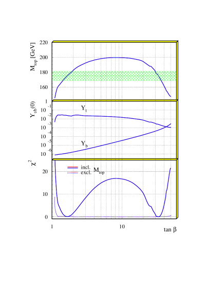
Figure 1: The top quark mass as function of ${\tan\beta}$ (top) for values of ${m_{0}},{m_{1/2}}~{}\approx 1$ TeV. The dependence shown is mainly determined by the $b-\tau$ Yukawa coupling unification. The middle part shows the corresponding values of the Yukawa coupling at the GUT scale and the lower part the $\chi^{2}$ values. If the top constraint (${m_{t}}=175\pm 6$, horizontal band) is not applied, all values of ${\tan\beta}$ between 1.2 and 50 are allowed (thin dotted lines at the bottom), but if the top mass is constrained to the experimental value, only the regions $1\leq{\tan\beta}\leq 3$ and $20\leq{\tan\beta}\leq 40$ are allowed.

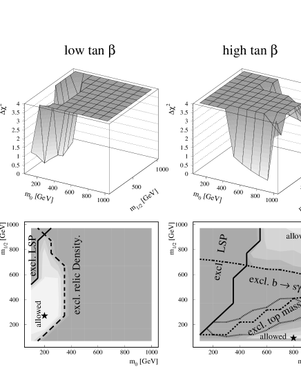
Figure 2: Contours of the $\chi^{2}$-distribution for the low and high ${\tan\beta}$ solutions. The different shades indicate steps of $\Delta\chi^{2}=1$, so basically only the light shaded region is allowed. The stars indicate the optimum solution. Contours enclose domains excluded by the particular constraints used in the analysis.

input data	$\Rightarrow$	Fit parameters
$\alpha_{1},\alpha_{2},\alpha_{3}$	min.	$M_{\rm GUT}$ , $\alpha_{\rm GUT}$
$m_{t}$  $m_{b}$ , $m_{\tau}$	$\chi^{2}$	$Y_{t}^{0},~{}Y_{b}^{0}=Y_{\tau}^{0}$
$M_{Z}$		$m_{0},~{}m_{1/2},~{}\mu$,  $\tan\beta$
$b\rightarrow s\gamma$		$A_{0}$
$\tau_{universe}$

Table 1: Summary of input data and fit parameters, which are determined from a global fit. They are mainly sensitive to the following input data: The GUT scale $M_{\rm GUT}$   and corresponding coupling constant $\alpha_{\rm GUT}$   are determined from gauge coupling unification, the Yukawa couplings $Y_{(t,b,\tau)}^{0}$ at the GUT scale from the masses of the 3th generation, $\mu$ from electroweak symmetry breaking (EWSB) and ${\tan\beta}$ from $b\tau$-unification. For the low ${\tan\beta}$ scenario the trilinear coupling $A_{0}$ is not very relevant, but for large ${\tan\beta}$ it is determined by ${b\rightarrow s\gamma}$ and $b\tau$-unification. The scalar- and gaugino masses $(m_{0},m_{1/2})$ enter in all observables.

Fitted SUSY parameters and masses in GeV
Symbol	low ${\tan\beta}$	high ${\tan\beta}$
$m_{0}$,  $m_{1/2}$	230,  225	850, 115
$\mu({M_{Z}})$, $\tan\beta$	-880, 1.7	-190, 30
$Y_{t}({m_{t}})$, $A_{t}({M_{Z}})$	0.008, -370	0.006, 86
$\tilde{\chi}^{0}_{1}$, $\tilde{\chi}^{0}_{2}$	96, 194	47, 92
$\tilde{\chi}^{0}_{3}$, $\tilde{\chi}^{0}_{4}$	509, 519	414, 417
$\tilde{\chi}^{\pm}_{1}$, $\tilde{\chi}^{\pm}_{2}$	194, 518	92, 422
$\tilde{g}$, $\tilde{q}$, $\tilde{l}$	558, 545, 563	300, 885, 854
$h,~{}H$	74, 673	109, 624
$A,~{}H^{\pm}$	680, 684	624, 630

Table 2: Values of the fitted SUSY parameters (upper part) and corresponding susy masses (lower part) for low and high ${\tan\beta}$ solutions using the new input data discussed in the text.

2 Results

The most restrictive constraints are the coupling constant unification and the requirement that the unification scale has to be above $10^{15}$ GeV from the proton lifetime limits, assuming decay via s-channel exchange of heavy gauge bosons. They exclude the SM $\!{}^{{\bf?}}$ as well as many other models $\!{}^{{\bf?}}$.
Constraints from $b-\tau$ unification
The requirement of bottom-tau Yukawa coupling unification strongly restricts the possible solutions in the ${m_{t}}$ versus ${\tan\beta}$ plane. For $m_{t}=175\pm 6$ GeV only two regions of ${\tan\beta}$ give an acceptable $\chi^{2}$ fit, as shown in the bottom part of fig. 1. The curves in the upper parts are determined by the relations between top and bottom masses and ${\tan\beta}$:

$$m_{t}^{2}=4\pi Y_{t}v^{2}\frac{\tan^{2}\beta}{1+\tan^{2}\beta}$$ (1)

$$m_{b}^{2}=4\pi Y_{b}v^{2}\frac{1}{1+\tan^{2}\beta}$$ (2)

For increasing ${\tan\beta}$ $m_{t}^{2}$ reaches quickly its plateau $4\pi Y_{t}v^{2}$; for large ${\tan\beta}$ $Y_{b}$ has to compensate the $1/\tan^{2}\beta$ term, so it quickly increases (see middle part). But then the (negative) $Y_{b}$ contributions to the running of $Y_{t}$ from loops involving both top and bottom cannot be neglected anymore, which decrease $Y_{t}$ and correspondingly the top mass for high ${\tan\beta}$.
Electroweak Symmetry Breaking (EWSB)
Radiative corrections can trigger spontaneous symmetry breaking in the electroweak sector. In this case the Higgs potential does not have its minimum for all fields equal zero, but the minimum is obtained for non-zero vacuum expectation values of the fields. Solving ${M_{Z}}$ from the minimum of the Higgs potential yields:

$$\frac{{M_{Z}}^{2}}{2}=\frac{m_{1}^{2}+\Sigma_{1}-(m_{2}^{2}+\Sigma_{2})\tan^{2}\beta}{\tan^{2}\beta-1},$$ (3)

where $m_{1,2}$ are the mass terms in the Higgs potential and $\Sigma_{1}$ and $\Sigma_{2}$ their radiative corrections. Note that the radiative corrections are needed, since unification at the GUT scale with $m_{1}=m_{2}$ would lead to $M_{Z}<0$. In order to obtain $M_{Z}>0$ one needs to have which happens at low energy since $\Sigma_{2}$ ($\Sigma_{1}$) contains large negative corrections proportional to $Y_{t}$ ($Y_{b}$) and $Y_{t}\gg Y_{b}$. Electroweak symmetry breaking for the large ${\tan\beta}$ scenario is not so easy, since eq. 3 can be rewritten as:

$$\tan^{2}\beta = \frac{m_{1}^{2}+\Sigma_{1}+\frac{1}{2}M_{Z}^{2}}{m_{2}^{2}+\Sigma_{2}+\frac{1}{2}M_{Z}^{2}}.$$ (4)

For large ${\tan\beta}$ $Y_{t}\approx Y_{b}$, so $\Sigma_{1}\approx\Sigma_{2}$. Eq. 4 then requires the starting values of $m_{1}$ and $m_{2}$ to be different in order to obtain a large value of $\tan\beta$, which could happen if the symmetry group above the GUT scale has a larger rank than the SM, like e.g. SO(10)$\!{}^{{\bf?}}$. In this case the quartic interaction (D-) terms in the Higgs potential can generate quadratic mass terms, if the Higgs fields develop non-zero v.e.v’s after spontaneous symmetry breaking.

Alternatively, one has to assume the simplest GUT group $SU(5)$, which has the same rank as the SM, so no additional groups are needed to break SU(5) and consequently no D-terms are generated. In this case EWSB can only be generated, if $Y_{b}$ is sufficiently below $Y_{t}$, in which case the splitting between $m_{1}$ and $m_{2}$ at low energies is sufficient to generate EWSB. The resulting SUSY mass spectrum is not very sensitive to the two alternatives for obtaining $m_{1}^{2}+\Sigma_{1}>m_{2}^{2}+\Sigma_{2}$: either through a splitting between $m_{1}$ and $m_{2}$ already at the GUT scale via D-terms or by generating a difference via the radiative corrections.
Discussion of the remaining constraints
In fig. 2 the total $\chi^{2}$ distribution is shown as a function of ${m_{0}}$ and ${m_{1/2}}$ for the two values of ${\tan\beta}$ determined above. One observes minima at ${m_{0}},{m_{1/2}}$ around (200,270) and (800,90), as indicated by the stars. These curves were still produced with the data from last year. With the new coupling constants one finds slightly different minima, as given in table 2. In this case the minimum $\chi^{2}$ is not as good, since the fit wants ${\alpha_{s}}\approx 0.125$, i.e. about 1.6$\sigma$ above the measured LEP value and the calcaluted ${b\rightarrow s\gamma}$ rate is above the experimental value too, if one takes as renormalization scale $\mu\approx 0.65m_{b}$. At this scale the next higher order corrections, as calculated by $\!{}^{{\bf?}}$, are minimal.

The contours in fig. 2 show the regions excluded by different constraints used in the analysis:
LSP Constraint: The requirement that the LSP is neutral excludes the regions with small $m_{0}$ and relatively large $m_{1/2}$, since in this case one of the scalar staus becomes the LSP after mixing via the off-diagonal elements in the mass matrix. The LSP constraint is especially effective at the high $\tan\beta$ region, since the off-diagonal element in the stau mass matrix is proportional to $A_{t}m_{0}-\mu\tan\beta$.
$b\rightarrow s\gamma$ Rate: At low $\tan\beta$ the $b\rightarrow s\gamma$ rate is close to its SM value for most of the plane. The charginos and/or the charged Higgses are only light enough at small values of $m_{0}$ and $m_{1/2}$ to contribute significantly. The trilinear couplings were found to play a negligible role for low $\tan\beta$ . However, for large ${\tan\beta}$ the trilinear coupling needs to be left free, since it is difficult to fit simultaneously ${b\rightarrow s\gamma}$, $m_{b}$ and $m_{\tau}$. The reason is that the corrections to $m_{b}$ are large for large values of $\tan\beta$ due to the large contributions from $\tilde{g}-\tilde{q}$ and $\tilde{\chi}^{\pm}-\tilde{t}$ loops proportional to $\mu{\tan\beta}$. They become of the order of 10-20%. In order to obtain $m_{b}(M_{Z})$ as low as 2.84 GeV, these corrections have to be negative, thus requiring $\mu$ to be negative. The $b\rightarrow s\gamma$ rate is too large in most of the parameter region for large $\tan\beta$ , because of the dominant chargino contribution, which is proportional to $A_{t}\mu$. For positive (negative) values of $A_{t}\mu$ this leads to a larger (smaller) branching ratio $BR(b\rightarrow s\gamma)$ than for the Standard Model with two Higgs doublets. In order to reduce this rate one needs $A_{t}(M_{Z})>0$ for $\mu<0$. Since for large $\tan\beta$ $A_{t}$ does not show a fix point behaviour, this is possible.
Relic Density: The long lifetime of the universe requires a mass density below the critical density, else the overclosed universe would have collapsed long ago. This requires that the contribution from the LSP to the relic density has to be below the critical density, which can be achived if the annihilation rate is high enough. Annihilation into electron-positron pairs proceeds either through t-channel selectron exchange or through s-channel $Z^{0}$ exchange with a strength given by the Higgsino component of the lightest neutralino. For the low $\tan\beta$ scenario the value of $\mu$ from EWSB is large$\!{}^{{\bf?}}$. In this case there is little mixing between the higgsino- and gaugino-type neutralinos as is apparent from the neutralino mass matrix: for $|\mu|\gg M_{1}\approx 0.4m_{1/2}$ the mass of the LSP is simply $0.4m_{1/2}$ and the “bino” purity is 99%$\!{}^{{\bf?}}$. For the high $\tan\beta$ scenario $\mu$ is much smaller and the Higgsino admixture becomes larger. This leads to an enhancement of $\tilde{\chi}^{0}-\tilde{\chi}^{0}$ annihilation via the s-channel Z boson exchange, thus reducing the relic density. As a result, in the large ${\tan\beta}$ case the constraint $\Omega h_{0}^{2}<1$ is almost always satisfied unlike in the case of low ${\tan\beta}$.

Figure 3: The mass of the lightest CP-even Higgs as function of the top mass at Born level (dotted lines), including complete one-loop contributions of all particles (dashed lines). Two-loop contributions reduce the one-loop corrections significantly as shown by the dashed area (the upper boundary corresponds to $\mu>0$, the lower one to $\mu<0$). The solid line just below the dashed line is the one-loop prediction from the third generation only, which apparently gives the main contribution. The upper scale indicates the value of ${\tan\beta}$, as calculated from the top mass by the requirement of $b\tau$-unification.

3 Discovery Potential at LEP II

Table 2 shows that charginos, neutralinos and the lightest Higgs belong to the lightest particles in the MSSM. Charginos are expected to be easy to discover, since they will be pair produced with a large cross section of several $pb$ and lead to events with characteristic decays similar to $W^{\pm}$ pairs plus missing energy.

The Higgs mass depends on the top mass as shown in fig. 3. Here the most significant second order corrections to the Higgs mass have been incorporated $\!{}^{{\bf?}}$, which reduces the Higgs mass by about 15 GeV $\!{}^{{\bf?}}$. In this case the Higgsmass is below 90 GeV, provided the top mass is below 180 GeV (see fig. 3), which implies that the foreseen LEP energy of 192 GeV is sufficient to cover the whole parameter space.

4 Summary

The new precise determinations of the strong coupling constant ${\alpha_{s}}=0.120\pm 0.003$ are slightly below the preferred CMSSM fit value of about 0.125. In addition, the ${b\rightarrow s\gamma}$ value of $(2.32\pm 0.6)10^{-4}$ is below the predicted values, at least for the SM $(3.2\cdot 10^{-4})$ and low ${\tan\beta}$ scenario of the MSSM. For high ${\tan\beta}$ the gluino-neutralino loop can decrease ${b\rightarrow s\gamma}$ somewhat.

The lightest particles preferred by these fits are charginos and higgses. The latter has a mass below 90 GeV for a top mass below 180 GeV in the low ${\tan\beta}$ scenario, which is within reach of LEP II.

It should be noted that recent speculation about evidence for SUSY from the $ee\gamma\gamma$ event observed by the CDF collaboration$\!{}^{{\bf?}}$, the too high value of $R_{b}$$\!{}^{{\bf?},{\bf?},{\bf?}}$ and the ALEPH 4-jet events$\!{}^{{\bf?},{\bf?}}$ all pointed to a SUSY parameter space inconsistent with the CMSSM, since they require very light sparticles (selectron, stop, chargino and/or neutralino). However, the $R_{b}$ anomaly has practically disappeared$\!{}^{{\bf?},{\bf?}}$ and the ALEPH 4-jet events observed at 135 GeV have not been confirmed at 161 GeV$\!{}^{{\bf?}}$.
Acknowledgments:
Thanks go to my close collaborators R. Ehret, D. Kazakov, and Ulrich Schwickerath during this analysis. This work was partly done during a sabbatical and support from the Volkswagen-Stiftung (Contract I/71681) is greatly appreciated.
References:

References

-
[1]
For references see e.g. the review papers:
H.-P. Nilles, Phys. Rep. 110 (1984) 1;
H.E. Haber, G.L. Kane, Phys. Rep. 117 (1985) 75; W. de Boer, Progr. in Nucl. and Particle Phys., 33 (1994) 201. - [2] M. Schmelling, these proceedings.
- [3] W. de Boer, A. Dabelstein, W. Hollik, W. Mösle and U. Schwickerath, hep-ph/9609209
- [4] A. Blondel, these proceedings.
- [5] M. Misiak, these proceedings.
- [6] W. de Boer et al., Z. Phys. C71 (1996) 415.
- [7] U. Amaldi, W. de Boer, and H. Fürstenau, Phys. Lett. B260 (1991) 447;
- [8] U. Amaldi,et al., Phys. Lett. B281 (1992) 374.
- [9] H. Murayama, M. Olechowski, and S. Pokorski, Phys. Lett. B371 (1996) 57 and ref. therein.
- [10] A.V. Gladyshev et al. IEKP-KA/96-03, hep-ph/9603346 and references therein.
- [11] M.Carena et al., hep-ph/9602250
- [12] G. Kane, these proceedings; S. Dimopoulos et al, Phys. Rev. D54 (1996) 3283.
- [13] W. de Boer, these proceedings.
- [14] J. Marco, these proceedings.
- [15] S. Pokorski, these proceedings.
- [16] Presentations by the 4 LEP Collaborations at the LEPC Meeting, CERN, Oct. 8, 1996.