Chiral Symmetry Breaking in Axial Gauge QCD from the Dyson-Schwinger Equations

Abstract

We investigate the nonperturbative behaviour of the quark propagator in axial gauge using a truncation of the Dyson-Schwinger equations which respects the Ward-Takahashi identity and multiplicative renormalisability. We demonstrate that above a critical coupling $\alpha_{c}$, which depends on the form of the gluon propagator, one can obtain massive solutions for both explicit and dynamically generated quark masses. The stability of these is discussed in the context of the Cornwall-Jackiw-Tomboulis effective action.

I Introduction

The Dyson-Schwinger equations (DSEs), in effect the functional Euler-Lagrange equations of quantum field theory, provide a natural framework for investigating nonperturbative Green functions. Whilst this infinite tower of equations encodes all information relating Green functions of different order, their use was restricted until quite recently because of the often brutal approximations which were necessary to render them soluble. A great deal of progress has been made subsequently, much of which is reviewed in Ref. [1], which comprehensively covers QED, QCD and applications to hadronic physics. We will be concerned with the DSE for the inverse quark propagator, shown diagrammatically in Fig.1, which relates the fully dressed quark and gluon propagators to the complete quark-gluon vertex. Early studies replaced the gluon propagator and quark-gluon vertex by their perturbative expressions, violating the the Ward-Takahashi identity (WTI) connecting the quark propagator to the vertex and destroying the universality of the QCD coupling constant. More recently, Bashir and Pennington, extending previous work by Curtis and Pennington, have shown how imposing the constraint that the critical coupling marking the onset of chiral symmetry breaking be gauge covariant places strong restrictions on the transverse component of the quark-gluon vertex [2, 3]. The longitudinal part can of course be determined from the WTI [4]. Whilst studies of DSEs in such a scheme appear to be at an early stage due to the complex nature of the expressions involved, the weaker condition of requiring that multiplicative renormalisability be respected, which also puts strong constraints on the transverse vertex, has been used widely and with considerable success; particularly in massive quenched strongly-coupled ${\rm QED}_{4}$ [5].

Lattice simulations hold out the possibility of a first principles determination of nonperturbative propagators [6]. However, their use has been hampered because with current technology they are unreliable below $\sim 1$ GeV, where the most interesting and novel behaviour is expected to lie. Additionally, gauge fixing on the lattice reduces the number of gauge configurations available for analysing whilst at the same time introducing ambiguities due to the presence of Gribov copies. The latter could be avoided by implementing an axial gauge fixing procedure on the lattice, rather than the more usual Landau gauge, but unfortunately there are then further complications associated with imposing periodic boundary conditions. It would seem therefore that at the present time DSEs are the most reliable tool for studying the infrared behaviour of propagators in the continuum limit.

In what follows we consider the quark propagator $S(p)$, given in terms of functions $F(p)$ and $M(p)$ by

$$S^{-1}(p)=\frac{\gamma.p-M(p)}{F(p)}$$ (1)

and with the form for the quark-gluon vertex specified by Curtis and Pennington [3]. In axial gauge the propagator may have additional structure of the the type $\gamma.n(\gamma.p\,G+H)$, $n$ being the four-vector appearing in the axial gauge fixing condition $n_{\mu}A^{\mu}=0$. The addition of such terms, although potentially important, results in a large increase in the complexity of the problem, and represents a direction for future research. We choose also to work with $p.n=0$ as a further condition on the specification of the gauge, again for practical reasons to make the equations more tractable. The general gauge dependence of the quark propagator is extremely interesting, but lies beyond the scope of present DSE studies except in the case of ${\rm QED}_{4}$ in covariant gauges, where details are now beginning to emerge [7, 8]

II The Quark DSE

The quark DSE for $S(p)$ at spacelike momenta, $-p^{2}>0$, may be written formally as

$$1=\gamma.p\,S(p)-\frac{\alpha C_{f}}{4\pi}\int D_{\mu\nu}(k-p)S(k)\Gamma^{\nu}(k,p)S(p)\,d^{4}k,$$ (2)

where $\alpha$ is the strong coupling, $C_{f}$ is the quark Casimir, $D_{\mu\nu}(k-p)$ is the full gluon propagator and $\Gamma^{\nu}(k,p)$ is the quark-gluon vertex. The ansatz which we shall use for the latter function is

$$\Gamma^{\nu}(k,p)=\Gamma^{\nu}_{L}(k,p)+\Gamma^{\nu}_{T}(k,p),$$ (3)

with

$$\Gamma^{\nu}_{L}(k,p) = {\gamma^{\nu}\over 2}\left({1\over{F(k)}}+{1\over{F(p)}}\right)+{1\over 2}\frac{(k+p)^{\nu}(\gamma.k+\gamma.p)}{k^{2}-p^{2}}\left({1\over{F(k)}}-{1\over{F(p)}}\right)$$ (4)

$$- \left({{M(k)}\over{F(k)}}-{{M(p)}\over{F(p)}}\right)\frac{(k+p)^{\nu}}{k^{2}-p^{2}}$$ (5)

and

$$\Gamma^{\nu}_{T}(k,p) = {1\over 2}\left({1\over{F(k)}}-{1\over{F(p)}}\right)\frac{\gamma^{\nu}(k^{2}-p^{2})-(k+p)^{\nu}(\gamma.k-\gamma.p)}{D(k,p)},$$ (6)

in which $D(k,p)$ is a regular function of $k$ and $p$ which behaves as $k^{2}$ for $k^{2}\gg p^{2}$. The transverse contribution $\Gamma_{T}$ cannot be specified uniquely. However, its form may be strongly constrained by demanding that the quark propagator respects the requirements of multiplicative renormalisability, as described by Curtis and Pennington. We have described previously the insensitivity of solutions of the quark DSE to the precise form of $D(k,p)$ [9] and will adopt here

$$D(k,p)=\frac{(k^{2}-p^{2})^{2}+\left[M^{2}(k)+M^{2}(p)\right]^{2}}{k^{2}+p^{2}},$$ (7)

which guarantees that multiplicative renormalisability is respected to all orders in leading- and next-to-leading logarithms. This is the form suggested by Curtis and Pennington in their important study of the structure of the transverse vertex and is the most widely used in recent DSE work. Upon substituting expressions (6) for the vertex into the quark DSE, it is clear that in the absence of any mass terms, i.e. with $M(p)=0$, there is a single linear integral equation for the wavefunction $F(p)$ which looks generically like

$$1=F(p)-\beta\int^{\Lambda}\frac{\Delta_{1}(k,p)F(p)+\Delta_{2}(k,p)F(k)}{k^{2}}Z\left((k-p)^{2}\right)d^{4}k,$$ (8)

where the shorthand $4\pi\beta=\alpha C_{f}$ has been used and the kernels $\Delta_{1}(k,p)$ and $\Delta_{2}(k,p)$ are functions to be specified. $Z(k^{2})$ represents the nonperturbative aspect of the gluon propagator, as will be described in more detail in the next section. The form of equation (8) follows from noting that the integral on the right-hand side of the DSE is proportional to $F(p)F(k)$, whilst the vertex contains terms which are inversely proportional to $F(p)$ or $F(k)$ separately. $\Lambda$ is an ultraviolet regulator in the guise of a sharp momentum cutoff.

In earlier work we elected to evaluate the angular integrals analytically by means of a shift in variables to remove the angular dependence from the gluon propagator and then by assuming that $F(p)$ was sufficiently flat that the approximation $F\left((k-p)^{2}\right)\approx F(k^{2}+p^{2})$ could be made [9]. This idea had been used previously in a study of the gluon propagator in axial gauge [10], but its validity is highly questionable and we shall show that it leads to spurious errors in the solution for $F(p)$.

We have indicated elsewhere how unique, finite solutions to (8) exist provided that the function $\phi(p)$ defined by

$$\phi(p)=1-\beta\int\frac{\Delta_{1}(k,p)}{k^{2}}Z(k^{2})\,d^{4}k$$ (9)

is nonzero for all $p^{2}$ [9]. Since $\Delta_{1}(k,p)$ and therefore $\phi(p)$ is independent of $F(p)$, this implies the existence of a value of $\beta$ for which $\phi$ can be made zero and which results in the breakdown of solutions for $F(p)$ with $M(p)=0$. If the integral in $\phi(p)$ is positive, this $\beta$ defines a critical value of the strong coupling $\alpha$ which is interpreted as signalling chiral symmetry breaking. When the mass function $M(p)$ is reintroduced, $\phi(p)$ is changed to become

$$\phi^{\prime}(p)=1-\beta\int\frac{\Delta_{1}(k,p)}{k^{2}+M^{2}(k)}Z(k^{2})\,d^{4}k,$$ (10)

which has an integrand suppressed at the origin relative to $\phi(p)$ provided $M(k^{2}\rightarrow 0)\neq 0$. This lifts the condition $\phi(p)=0$ and means that solutions for $F$ can be recovered beyond the critical coupling exhibited above. $M(p)$ may be introduced by hand as an explicit quark mass, or it may be generated by the dynamics of the quark-gluon interactions.

The $F(p)$ appearing in equation (8) is a bare quantity which has an inherent dependence on the ultraviolet regulator $\Lambda^{2}$ and should be written strictly as $F(p^{2};\Lambda^{2})$. Its subtractive renormalisation follows from introducing a renormalisation constant $F_{\mu}(\mu^{2},\Lambda^{2})$ so that $\widetilde{F}(p^{2};\mu^{2})=F_{\mu}(\mu^{2},\Lambda^{2})F(p^{2};\Lambda^{2})$ is the renormalised wavefunction which depends on $p^{2}$ and a renormalisation point $\mu^{2}$ at which we impose the boundary condition $\widetilde{F}(\mu^{2};\mu^{2})=1$, corresponding to the free propagator. The numerical solution of the resulting integral equation for $F(p)$ is amenable to a number of methods. The one used here is to map the integration over $k$ onto a finite logarithmic mesh, which entails both infrared and ultraviolet cutoffs whose effect will need to be determined. Following this the integral is replaced by a discrete sum so that

$$\int K(p,k)f(k)\,dk\approx\sum_{j=1}^{N}K(p_{i},k_{j})f(k_{j})\,\omega_{j}$$ (11)

where the weights $\omega_{j}$ are chosen according to a Gaussian quadrature rule and $N$ is the number of grid points used.

At each value of $(p,k)$ it is necessary to have also a numerical evaluation of the angular integrals since the gluon contains the dependence $Z\left((k-p)^{2}\right)=Z(k^{2}+p^{2}-2pk\cos\theta)$. With these steps, the solution of (8) becomes equivalent to determining the elements $f(p_{i})$ which satisfy $N$ simultaneous linear equations of the general type

$$f(p_{i})+\sum_{j=1}^{N}K(p_{i},k_{j})f(k_{j})\,\omega_{j}=g(p_{i}).$$ (12)

The accuracy of the discretised approximation can be found retrospectively by iterating the equation for $F(p)$ with increasing $N$ to ensure that the error is small.

III Chiral Solutions

The kernels $\Delta_{1}(p,k)$ and $\Delta_{2}(p,k)$ do not depend on either $F(p)$ or $Z(k^{2})$ and are given in the appendix. An expansion of $\Delta_{1}$ and $\Delta_{2}$ for $k^{2}\gg p^{2}$ reveals that the integrand involving $\Delta_{1}$ decreases as a power $(k^{2})^{-\delta}Z(k^{2})$ with $\delta=3/2$ and the integrals involving it are finite. On the other hand $\Delta_{2}$ behaves as $(k^{2})^{0}$ for $k^{2}\gg p^{2}$ and the finiteness of its contribution depends on the asymptotic behaviour of $F(k)$ and $Z(k^{2})$. We must specify the precise form of $Z(k^{2})$ to be used to determine the critical coupling and numerical solutions for $F(p)$. An additional point worth noting is that in a scheme where MR is not enforced, the divergence in the equations is present in the $\Delta_{1}$ rather than the $\Delta_{2}$ terms. The coefficient of the divergence is a function of $p^{2}$ and cannot be removed by a straightforward subtraction.

In one of the first serious studies of the gluon DSE, Baker, Ball and Zachariasen (BBZ) examined the consequences of a gluon propagator which had the same tensor structure as the perturbative one combined with the scalar function $Z(k^{2})$ representing the nonperturbative dynamics so that [11]

$$D_{\mu\nu}(k^{2})=-\frac{Z(k^{2})}{k^{2}}\left(g_{\mu\nu}-\frac{k_{\mu}n_{\nu}+k_{\nu}n_{\mu}}{k.n}+n^{2}\frac{k_{\mu}k_{\nu}}{(k.n)^{2}}\right).$$ (13)

More generally in axial gauge the propagator could contain the additional contribution

$$D^{\prime}_{\mu\nu}(k^{2})=\rho_{2}(k^{2})\left(g_{\mu\nu}-\frac{n_{\mu}n_{\nu}}{n^{2}}\right),$$ (14)

where $\rho_{2}(k^{2})$ is a further function to be determined. The value of taking (13) alone is that the terms in the gluon DSE involving the full four-gluon vertex are projected out, resulting in a considerable simplification. Of course, the main attraction of axial gauge is the absence of the ghost fields, which removes one of the diagrams involved in the gluon equation and means that the Ward-Slavnov-Taylor identity for the quark-gluon vertex can be replaced by the Ward-Takahashi identity, enabling us to use the expression for the vertex in (6), which was originally proposed for QED, without further approximation. The solutions found by BBZ, which incorporated only the longitudinal contribution to the quark-gluon vertex, exhibited a $Z(k^{2})$ which diverged strongly as $(k^{2})^{-1}$ in the infrared and which had the asymptotic limit $(\ln k^{2})^{-11/16}$, which disagrees with renormalisation group improved one-loop perturbation theory. However, in attempts to describe phenomenology by the exchange of one or more soft gluons, infrared divergences arise unless the gluons are softer than $(k^{2})^{-1}$ as $k^{2}\rightarrow 0$. On the other hand, the axial gauge propagator cannot be nonsingular at $k^{2}=0$. The remaining possibility is for a cut solution which behaves as $(k^{2})^{-\zeta}$ with $0<\zeta<1$. The nonlinearity of the gluon DSE suggests that there may exist alternative solutions even within the same truncation schemes.

A very successful phenomenology of diffractive scattering, elastic scattering, the gluon structure function and total cross-sections results from the idea, first suggested by Landshoff and Nachtmann [12], of a process-independent softening of the gluon propagator in the infrared domain [13]. Models of diffractive scattering, such as two-gluon exchange, suffer from infrared divergences if the propagator is not softer than $1/k^{2}$ as $k^{2}\rightarrow 0$. In particular, it is not possible to obtain the experimentally observed slope of the hadronic scattering cross-sections in the $t$-channel with an extremely infrared-divergent gluon. Whilst a strongly infrared-singular propagator might well be relevant to the question of the nature of confinement, a softer behaviour is far more phenomenologically efficacious.

With this is mind, we wish to examine the consequences of a gluon propagator which is less singular than the one suggested by BBZ and which may therefore be phenomenologically relevant. Several alternatives are considered. As indicated above, it is believed that the gluonic wavefunction cannot be singular at the origin and the perturbative (quenched) propagator with $Z_{a}(k^{2})=1$ thus provides one limiting case. At the other extreme, one could have a propagator with no singularity at the origin, i.e. with $Z(k^{2})=k^{2}$ as $k^{2}\rightarrow 0$. Of course, the gluon cannot behave like this in the ultraviolet regime and it is necessary to introduce a scale $\mu^{2}$ which marks the transition from the nonperturbative to the perturbative region. Perturbatively, $Z(k^{2})$ runs as $[\ln k^{2}]^{-1}$ asymptotically. In order to reproduce this behaviour and to have $Z(k^{2}=\mu^{2})$ equal for all choices of the propagator, we take as our second ansatz

$$Z_{b}(x^{2})=\cases{x^{2},&$x^{2}\leq 1$\cr[\ln(e-1+x^{2})]^{-1},&$x^{2}>1$\cr}$$ (15)

with $x^{2}\mu^{2}=k^{2}$.

$Z_{a}$ and $Z_{b}$ represent two extreme alternatives and an intermediate between them is required. Ideally this should share the correct UV behaviour of $Z_{b}$ and lie between $Z_{a}$ and $Z_{b}$ for $k^{2}<\mu^{2}$. One possibility, which does have these properties, has phenomenologically desirable infrared behaviour and which can be applied successfully to reproduce the experimental data for $p-p$ scattering is that proposed by Cudell and Ross [14]:

$$Z_{c}(x^{2})=\frac{x^{2}}{0.88(x^{2})^{0.22}-0.59(x^{2})^{0.86}+0.95x^{2}\ln(2.1x^{2}+4.1)}.$$ (16)

This was derived originally from a study of the nonlinearity of the gluon DSE, which admits the existence of more than one solution. That particular analysis is flawed because of a sign error [18], but the phenomenologically attractive properties of equation (16) plus its position between $Z_{a}$ and $Z_{b}$ in the infrared domain make it an ideal ansatz for present puurposes.

The broad shape of the curves obtained for $F(p)$ is not affected by $Z(k^{2})$. They are illustrated in Fig. 2 with the choice $Z(k^{2})=Z_{c}(k^{2})$, for $\alpha=0.2,0.6,1.0,1.4$. These show a plateau for $p^{2}\leq\mu^{2}$, whose magnitude increases with $\alpha$, passing through the fixed point at $F(\mu^{2})=1$ and thereafter decreasing logarithmically as $(\ln p^{2})^{-\delta}$ with $\delta\approx 0.2$. The magnitude of $F(p)$ at large $p^{2}$ is suppressed as $\alpha$ is increased. In fact the value of $\alpha$ when $F(p)$ crosses the axis is coincident with the loss of solutions and corresponds to the critical coupling. In this case the critical value $\alpha_{c}$ was found to be $\alpha_{c}\approx 1.45$. For the alternatives for $Z(k^{2})$, $Z_{a}$ and $Z_{b}$ with the infrared limits $Z_{a}\rightarrow 1$ and $Z_{b}\rightarrow k^{2}$, we found $\alpha_{c}=0.9$ and $\alpha_{c}=1.9$ respectively. Interestingly the former of these is close to the $\alpha_{c}\approx 0.93$ which has been found in Landau gauge investigations of the quark propagator with a quenched gluon. When previously we used the approximation $F((p-k)^{2})\approx F(p^{2}+k^{2})$ to derive the integral equation for $F$, we found oscillations in the region $p^{2}\sim\mu^{2}$, whose magnitude grew with the coupling $\alpha$ until they dominated the solutions at $\alpha\sim\alpha_{c}$. They are completely absent from the present set of solutions and are thus clearly an artifact of the approximation. This is not too great a surprise, for whilst the derivative of $F(p)$ is indeed small for $p^{2}\ll\mu^{2}$ and $p^{2}\gg\mu^{2},F(p)$ changes rapidly near $p^{2}=\mu^{2}$.

The value of $\alpha_{c}$ is dominated by the infrared behaviour of the gluon and reduces with an increasingly singular gluon, which is an interesting effect in its own right. It suggests that the more rapidly the gluonic wavefunction increases at large distances, the lower the coupling at which chiral symmetry is dynamically broken. A determination as to whether the behaviour of the gluon is the major factor contributing to chiral symmetry breaking would require a more detailed analysis in which the quark and gluon DSEs were solved simultaneously. Conversely, it is quite plausible that an even softer gluon would not support chiral symmetry breaking at all. The test of whether the breakdown of chiral symmetry is the correct interpretation of $\alpha_{c}$ will follow from examining the more general case of a massive propagator.

IV The Massive DSE

Apart from the obvious complication of adding mass terms to the quark DSE, a feature which has been neglected frequently is the correct renormalisation prescription in the presence of a chiral symmetry breaking mass. This is nontrivial and of great importance to a fully self-consistent analysis of the solutions for $F(p)$ and $M(p)$. It is worth presenting the details here and we follow the notation used in Ref.[8]. In what follows, tildes denote renormalised quantities and primes denote regularised ones which depend on the UV regulator $\Lambda$.

The starting point is the renormalised inverse quark propagator $\widetilde{S}^{-1}(p)$ which can be written in terms of the renormalised current mass $m(\mu)$ and renormalised self-energy function $\widetilde{\Sigma}(p;\mu)$ as

$$\widetilde{S}^{-1}(p)=\gamma.p-m(\mu)-\widetilde{\Sigma}(p;\mu)=\left[\gamma.p-m_{0}(\Lambda)\right]Z_{2}(\mu,\Lambda)-\Sigma^{\prime}(p;\mu,\Lambda)$$ (17)

where all the dependencies have been shown explicitly, $Z_{2}(\mu,\Lambda)$ is the fermion renormalisation constant and $m_{0}(\Lambda)$ is the bare mass, which is zero in the massless limit of QCD. The self-energy can be decomposed into Dirac and scalar components as $\widetilde{\Sigma}(p;\mu,\Lambda)=\gamma.p\,\widetilde{\Sigma}_{1}(p;\mu,\Lambda)+\widetilde{\Sigma}_{2}(p;\mu,\Lambda)$ with a similar expression for $\Sigma^{\prime}$. At the renormalisation point the boundary condition

$$\left.\widetilde{S}^{-1}(p)\right|_{p^{2}=\mu^{2}}=\gamma.p-m(\mu)$$ (18)

is imposed. Upon inserting the decomposed self-energy into (17) and using (18), a comparison of the scalar terms and those involving $\gamma$ matrices reveals the relations between the renormalisation constant $Z_{2},\Sigma_{1},\Sigma_{2}$ and the bare and renormalised masses to be

$$Z_{2}(\mu,\Lambda)=1+\Sigma_{1}^{\prime}(\mu;\mu,\Lambda),$$ (19)

$$Z_{2}(\mu,\Lambda)m_{0}(\Lambda)=m(\mu)-\Sigma_{2}^{\prime}(\mu;\mu,\Lambda).$$ (20)

One can see from the second of these that in general for finite $\Lambda,m(\mu)=0$ does not necessarily imply that $Z_{2}(\mu,\Lambda)m_{0}(\Lambda)=0$ – this only happens when $m(\mu)=\Sigma_{2}^{\prime}(\mu;\mu,\Lambda)$. As the cutoff is removed however it is necessary that $\lim_{\Lambda\rightarrow\infty}Z_{2}m_{0}=0$ to ensure conservation of the axial current $j_{5}^{\mu}$ whose divergence is $\partial_{\mu}j_{5}^{\mu}=\partial_{\mu}(\bar{\psi}\gamma^{\mu}\gamma_{5}\psi)$. In practice we are forced to adopt a finite cutoff in numerical simulations, but one can check the dependence of $Z_{2}m_{0}$ on $\Lambda$ to verify that it does tend to zero in the limit.

Using (17) together with the relations between bare and renormalised quantities in (20) it is straightforward to show that the relation between the renormalised and regularised self-energies is

$$\widetilde{\Sigma}(p;\mu)=\Sigma^{\prime}(p;\mu,\Lambda)-\Sigma^{\prime}(\mu;\mu,\Lambda).$$ (21)

Writing the quark DSE in terms of renormalised quantities and recalling that in axial gauge $Z_{1}=Z_{2}$ we can see that the regularised self-energy is given by

$$\Sigma^{\prime}(p;\mu,\Lambda)=iZ_{2}(\mu,\Lambda)\frac{g^{2}C_{f}}{(2\pi)^{4}}\int^{\Lambda}d^{4}k\,\gamma^{\rho}\widetilde{S}(k)\widetilde{\Gamma}^{\sigma}(k,p)\widetilde{D}_{\rho\sigma}(k-p).$$ (22)

Taking the trace of both sides, or the trace after multiplying throughout by $\gamma.p$ yields a pair of coupled nonlinear equations for the two components of $\Sigma^{\prime}$. We wish to find the propagator in the form specified by (1), in terms of which the renormalisation condition for $M(p)$ is

$$\frac{M(p;\mu)}{\widetilde{F}(p;\mu)}=m(\mu)+\frac{M(p;\mu,\Lambda)}{F^{\prime}(p;\mu,\Lambda)}-\frac{M(\mu;\mu,\Lambda)}{F^{\prime}(\mu;\mu,\Lambda)}.$$ (23)

A Explicit Quark Mass

Explicit chiral symmetry breaking (ECSB) can be induced by introducing a non-zero renormalised quark current mass $m(\mu)$. Performing the traces in the DSE produces an equation for $F(p)$ of the form

$$1-\beta\int\frac{\Delta^{\prime}_{1}(\mu,k)}{k^{2}+M^{2}(k)}\,dk = F(p)-\beta F(p)\int\frac{\Delta^{\prime}_{1}(p,k)}{k^{2}+M^{2}(k)}\,dk$$ (24)

$$- \beta\int\frac{\Delta^{\prime}_{2}(p,k)-\Delta^{\prime}_{2}(\mu,k)}{k^{2}+M^{2}(k)}F(k)\,dk,$$ (25)

which remains linear in $F$, and a nonlinear equation for $M$ of the form

$$M(p)=m(\mu)F(p) + \beta Z_{2}(\mu,\Lambda)F(p)\int d^{4}k\,\frac{\chi_{1}(p,k)M(p)+\chi_{2}(p,k)M(k)}{k^{2}+M^{2}(k)}$$ (26)

$$- \beta Z_{2}(\mu,\Lambda)F(p)\int d^{4}k\,\frac{\chi_{1}(\mu,k)m(\mu)+\chi_{2}(\mu,k)M(k)}{k^{2}+M^{2}(k)}.$$ (27)

The kernels $\Delta^{\prime}_{1},\Delta^{\prime}_{2},\chi_{1}$ and $\chi_{2}$ have been relegated once more to the appendix and we will refer to the denominator $k^{2}+M^{2}(k)$ as $D_{1}(k,M)$ or simply as $D_{1}$. A complete determination of the quark propagator now entails the simultaneous solution of the two integral equations (25) and (LABEL:M_nonlin). The one for $F$ is simpler as it is still linear and can be solved, given a particular $M$, using the method outlined for the massless case. Equation (LABEL:M_nonlin) for $M$, being nonlinear, is more difficult and the approach taken was to introduce a generalisation in the form of a parameter $\lambda$ into the denominator $D_{1}$ which now becomes $D_{1}=k^{2}+\lambda M^{2}(k)$. The advantage of this is that $\lambda=0$ defines a linearised equation which is easy to solve and we can then increment $\lambda$ from 0 to 1, solving iteratively at each stage, to obtain the required solutions. The equations for $F$ and $M$ are solved alternately so that a given $F^{(i)}$ is used to obtain an approximation $M^{(i)}$ which is put back into the equation for $F$ to find $F^{(i+1)}$ etc. until convergence of both functions is achieved. The criterion used was that the error function defined by

$$\xi_{j}=\left|\frac{F_{j}^{(i)}-F_{j}^{(i+1)}}{F_{j}^{(i)}+F_{j}^{(i+1)}}\right|$$ (29)

satisfied $\xi_{j}<10^{-6}$ for all points $p_{j}$ at which $F$ was determined, with an equivalent condition for $M$.

As an illustration of the functions obtained, the equations were solved for $\mu^{2}=1$ with $m(\mu)=0.2$ using the Cudell-Ross form for the gluon propagator. The wavefunction $F$ and mass function $M$ are shown in Figs.3 and 4 respectively for $\alpha=0.4,0.8,1.2,1.6,2.0$. The cutoffs used were $\Lambda_{\rm IR}^{2}=10^{-6}$ and $\Lambda_{\rm UV}^{2}=10^{6}$ (the infrared cutoff was not expected to be important because all the integrands are strongly suppressed near $k^{2}=0$ and indeed there was no significant variation in any of the quantities calculated for $\Lambda_{\rm IR}^{2}=10^{-6},10^{-8},10^{-10}$ or $10^{-12}$).

The first point of note is that as advertised, incorporating $M(p)$ does allow us to recover solutions for $F(p)$ for $\alpha>\alpha_{c}\sim 1.45$. The magnitude of $M(p)$ as $p^{2}\rightarrow 0$ increases as $\alpha$ is increased, whilst the tail decreases with increasing $\alpha$ and becomes close to zero, although it appears never to cross the axis. Second, for a given $\alpha<\alpha_{c}$, $F(p)$ is both infrared suppressed and ultraviolet enhanced relative to the corresponding massless solution. Third, the large-$p^{2}$ variation of $F(p)$ with respect to $\alpha$ is reduced relative to the $M=0$ solutions.

In order to investigate the dependence of the solutions on the UV cutoff, the equations were re-solved with the same values of $\mu^{2}$ and $m(\mu)$ for each of $\log_{10}\Lambda^{2}=6.0,6.6,7.2...12.0$ and the values of $M(p^{2}\rightarrow 0),M(p^{2}=10^{6}),F(p^{2}\rightarrow 0)$ and $F(p^{2}=10^{6})$ established. These were used to find mean values and deviations which are shown in Fig.5 for $\alpha$ ranging from 0 to 2.0, where the error bars represent $\pm 1$ standard deviation. The mean value of $M(10^{6})$ is the only one to show appreciable variation, for $\alpha>1.5$. To eliminate the possibility of a systematic dependence on $\Lambda$, the correlation $\rho$ between each of the four quantities shown in Fig. 5 and $\ln\Lambda$ were evaluated. $\rho$ can take values between $\pm 1$ corresponding to perfect positive or negative correlations. In no case did it exceed ${\cal O}(10^{-3})$, which confirms that there is little if any $\Lambda$ dependence in the renormalised solutions.

B Dynamical Mass Generation

The ECSB solutions discussed above where $m(\mu)\neq 0$ are important – because quarks do after all have a mass – but the symmetry breaking has been put in “by hand”. To explore the transition between massless and massive phases, we must solve the equations for $m(\mu)=0$ (the chiral limit) to see if for $\alpha>\alpha_{c}$ a mass is generated dynamically. That is to say, can quark-gluon and self-interactions generate a mass from the initially massless theory? For $m(\mu)=0$ the equation for $M$ becomes

$$M(p)=\beta Z_{2}(\mu,\Lambda)F(p)\int^{\Lambda}\frac{\chi_{1}(p,k)M(p)+\left[\chi_{2}(p,k)-\chi_{2}(\mu,k)\right]M(k)}{k^{2}+M^{2}(k)},$$ (30)

where $\chi_{1}$ and $\chi_{2}$ are unchanged, as is the equation for $F$ apart from terms involving $M(\mu)=m(\mu)=0$ which vanish. As noted previously, for a finite cutoff, $m(\mu)=0$ does not imply that the product $Z_{2}m_{0}=0$. However, $\chi_{2}(\mu,k)$ is strongly suppressed for large $\mu^{2}$, leading to only a small residual value of $Z_{2}m_{0}$. This provides the basis for the success of the many studies which neglect the $\mu$-dependent part of the right-hand side of (30) and take $\mu^{2}=\Lambda_{\rm UV}^{2}$. They incur the undesirable side effect that $M(p)$ is barely down from its infrared magnitude even at $p^{2}=\Lambda^{2}$ [15], contrary to what one would expect for a dynamically generated mass term which should be small in the perturbative regime.

The new equation for $M$ was solved using a Powell hybrid method, after discretisation of the integrals, which is a variation of the Newton-Raphson technique which avoids the evaluation of derivatives [16]. The technique combines the advantages of a multidimensional root searching method with a minimisation of sum of squares to improve global convergence. This is convenient because it can be tailored to exclude the trivial $M=0$ solution. Solving the equations for $M$ and $F$ iteratively is problematic since for $\alpha>\alpha_{c}$, the existence of a solution for $F$ depends strongly on $M$. With a method which incorporates minimisation, we simply introduce a “penalty” to disfavour any intermediate $M$ which makes the equation for $F$ insoluble.

Once more the renormalisation point $\mu^{2}=1$ was used at which $M(p)$ must be zero to satisfy (23). Fig.6 shows the curves for $M$ obtained for $\alpha$ ranging from 1.4 to 2.0 with $\Lambda^{2}=10^{8}$. It was not possible to find solutions with $M\neq 0$ for $\alpha<1.39$, which is slightly lower than the critical $\alpha_{c}=1.45$. For $1.39<\alpha<1.45$ there are two possible sets of solutions for $F$ and $M$ – one having $M=0$ and the other $M\neq 0$. In Fig.6 we see that $M$ crosses the axis at $p^{2}=\mu^{2}$, attaining a minimum at $p^{2}\sim 2$ and then declining towards zero as $p^{2}\rightarrow\Lambda^{2}$. The size of $M$ in the infrared shows a familiar plateau with $M(0)$ increasing with $\alpha$. This is consistent with preventing a zero in the function $\phi(p)$ governing the existence of solutions for $F$. The depth of the minimum increases with $\alpha$ and $|M_{\rm min}|\approx 0.45\,|M(0)|$.

The corresponding curves for $F$, which are not shown, are very similar to those in Fig.3, but exhibit an interesting feature, namely that $F$ is quite insensitive to $\alpha$ in the presence of a dynamically generated mass. It appears that the dynamical $M$ holds $F$ close to its massless form immediately below $\alpha_{c}$. As $\alpha$ increases, the magnitude of $M$ increases to compensate, keeping $\phi(p)$ slightly above zero. The oscillations seen in $M$ have also been identified in strongly coupled massive quenched ${\rm QED}_{4}$, where they are much smaller in size.

The cutoff dependence of the solutions was tested for $\Lambda^{2}$ ranging between $10^{6}$ and $10^{12}$ and the renormalised $M$ again showed no significant change. The product $Z_{2}m_{0}$ was computed at each value of $\alpha$ and $\Lambda^{2}$ and the variation in this is shown in Fig.7. The slow decrease is striking and the reason for it lies in the nature of the integrands involved in calculating $Z_{2}$. Recalling that $Z_{2}(\mu,\Lambda)=1+\Sigma^{\prime}(\mu;\mu,\Lambda)$ we have, after some rearrangement, from (22)

$$Z_{2}(\mu,\Lambda)=\left\{1+\beta\int^{\Lambda}\frac{\Delta(\mu,k)}{k^{2}+M^{2}(k)}\right\}^{-1},$$ (31)

with $\Delta(p,k)=\Delta_{1}^{\prime}(p,k)F(p)+\Delta_{2}^{\prime}(p,k)F(k)$. Expanding the integrand in the case where $k^{2}\gg\mu^{2}$ we find

$$\frac{\Delta(p,k)}{k^{2}+M^{2}(k)}\sim\frac{2}{k\ln k^{2}}\left[1+F(k)\right],$$ (32)

where the limits $\theta_{1}=\theta_{3}=0$ and $2\theta_{2}=\theta_{4}=\pi Z(k^{2})$ have been used for the angular integrals (as they appear in the appendix), together with the leading term in $Z(k^{2})\sim\left[k^{2}\ln k^{2}\right]^{-1}$. The dominant part is thus $\Phi(k)\sim\left[k\ln k\right]^{-1}$ and the contribution of this to $Z_{2}$ is

$$I_{\Lambda}(\Phi)=\int_{a}^{\Lambda}\Phi(p,k)\,dk=\int_{a}^{\Lambda}\frac{dk}{k\ln k}$$ (33)

with $\Lambda^{2}\gg a^{2}\gg\mu^{2}$, giving $I(\Phi)=\ln\ln\Lambda-\ln\ln a$. So $Z_{2}m_{0}$ does go to zero with increasing $\Lambda$, but only as a double logarithm – the very slow decrease shown in Fig.7 which also shows a line fitting to $\ln\ln\Lambda$ to demonstrate the close agreement.

V Stability of the Solutions

The existence of simultaneous chiral symmetry preserving and chiral symmetry breaking solutions presents the question as to which is the physically important stable state. This problem can be addressed partially through the use of the Cornwall-Jackiw-Tomboulis (CJT) effective action $\Gamma_{\rm CJT}$ [17]. The condition $\frac{\delta\Gamma}{\delta S}=0$ locates the stationary points of the CJT action and is in fact equivalent to the DSE for the quark propagator. In other words, solutions to the fermion DSE automatically give $\frac{\delta\Gamma}{\delta S}=0$. At the stationary point, the CJT effective action can be written in terms of the propagator $S(p)$ as [1]

$$\Gamma_{\rm CJT}[S]={\rm Tr}\left[\ln S^{-1}\right]+{1\over 2}{\rm Tr}\left[1-S_{0}^{-1}S\right],$$ (34)

which may be evaluated for each of the sets of solutions where both $M=0$ or $M\neq 0$ are possible. The trace indicates integration over momenta and summation over all discrete indices. We can consider the difference $\Delta\Gamma$ between these, i.e.

$$\Delta\Gamma=\Gamma_{\rm CJT}[M=0]-\Gamma_{\rm CJT}[M\neq 0]$$ (35)

and a negative value with $\Delta\Gamma<0$ is interpreted as a signal that the occurrence of chiral symmetry breaking solutions lowers the energy of the vacuum and is preferred physically. Indeed, when $\Delta\Gamma$ was evaluated for explicit and dynamical quark masses, it was found that massive solutions are always favoured. This resolves the ambiguity for $1.39<\alpha<1.45$, where both a massless quark and one with a dynamically generated mass were possible. It appears that the latter is favoured.

One could go further and find the derivatives of $\Gamma_{\rm CJT}$ to ascertain the nature of the stationary point. However the CJT action is unsatisfactory because it is not bounded below. In particular one can show analytically that in Landau gauge the solutions to the gap equation with dynamical masses are unstable saddle points of the action although they still have $\Delta\Gamma<0$ as compared to the chiral solutions. It is not possible therefore to address conclusively the matter of the stability through the CJT formalism.

VI Concluding Remarks

Axial gauge solutions to the quark DSE have been found, in a truncation scheme which respects MR, for several possible forms for the gluon propagator in the infrared domain. These reproduce the familiar perturbative behaviour at high momentum and exhibit a critical value for the strong coupling $\alpha_{c}$, whose value decreases as the gluon propagator becomes increasingly infrared singular, independently of its ultraviolet running. Since chiral symmetry breaking is believed to be connected intimately with confinement, this provides further support, should such be required, that the confinement mechanism is linked closely to the infrared sector of QCD.

Above the critical coupling, solutions to the DSE can be recovered by the introduction of a quark mass, either dynamically or explicitly, as has been found in numerous covariant gauge studies. The correct treatment of the renormalisation of the massive case has not always been handled rigorously in the literature, despite the efforts of several authors, and yet it is crucially important in obtaining a self-consistent treatment of the DSE. It is worth reiterating that in numerical studies which inevitably involve a finite infrared regulator, it is not enough to simply set the bare and renormalised quark masses simultaneously to zero, although they must vanish as the cutoff is removed in order to ensure that the axial current is conserved.

Although we have discussed briefly the question of stability, as indicated the CJT formalism is not in itself a definitive tool. There have been a number of attempts to address this problem through alternative choices for the definition of the effective action and these represent an important direction for future investigation.

Finally, it is known how the ansatz used for the quark-gluon vertex can be improved through considerations of gauge invariance. Studies incorporating a suitable vertex should prove extremely interesting although they will require the solution of much more complicated integral equations. This is particularly so in axial gauge, and will become especially acute when the extra structure involving $\gamma.n$ is included in the form for the quark propagator.

A Integral equation kernels

Collected together here are the expressions for the various integral equation kernels which have been encountered earlier. The following shorthand notation has been adopted for the angular integrals:

$$\theta_{1} = \int_{0}^{\pi}Z(p^{2}+k^{2}-2pk\cos\theta)\sin^{2}\theta\cos\theta\,d\theta,$$ (A1)

$$\theta_{2} = \int_{0}^{\pi}Z(p^{2}+k^{2}-2pk\cos\theta)\sin^{2}\theta\,d\theta,$$ (A2)

$$\theta_{3} = \int_{0}^{\pi}Z(p^{2}+k^{2}-2pk\cos\theta)\cos\theta\,d\theta,$$ (A3)

$$\theta_{4} = \int_{0}^{\pi}Z(p^{2}+k^{2}-2pk\cos\theta)\,d\theta.$$ (A4)

For the massless case with the Curtis-Pennington vertex one has

$$\Delta_{1}(p,k) = -2pk^{2}\theta_{3}-4{k^{4}\over p}\theta_{1}-2{k^{4}\over p}\theta_{3}+4k^{3}\theta_{2}+4k^{3}\theta_{4}$$ (A5)

$$+ {1\over{D(p,k)}}\left[-4p^{2}k^{3}\theta_{2}+16pk^{4}\theta_{1}-8{k^{5}\over p}\theta_{1}-4k^{5}\theta_{2}\right]$$ (A6)

$$+ \frac{1}{k^{2}-p^{2}}\left[-2p^{3}k^{2}\theta_{3}+2p^{2}k^{3}\theta_{2}+4pk^{4}\theta_{1}+4pk^{4}\theta_{3}-2{k^{6}\over p}\theta_{3}+2k^{5}\theta_{2}\right],$$ (A7)

$$\Delta_{2}(p,k) = -2pk^{2}\theta_{3}-4{k^{4}\over p}\theta_{1}-2{k^{4}\over p}\theta_{3}+4k^{3}\theta_{2}+4k^{3}\theta_{4}$$ (A8)

$$+ {1\over{D(p,k)}}\left[4p^{2}k^{3}\theta_{2}-16pk^{4}\theta_{1}+8{k^{6}\over p}\theta_{1}+4k^{5}\theta_{2}\right]$$ (A9)

$$+ \frac{1}{k^{2}-p^{2}}\left[2p^{3}k^{2}\theta_{3}-2p^{2}k^{3}\theta_{2}-4pk^{4}\theta_{1}-4pk^{4}\theta_{3}+2{k^{6}\over p}\theta_{3}-2k^{5}\theta_{2})\right].$$ (A10)

In the massive case, the kernels appearing in the equation for $F$ are given by

$$\Delta^{\prime}_{1} = -2pk^{2}\theta_{3}-4{k^{4}\over p}\theta_{1}-2{k^{4}\over p}\theta_{3}+4k^{3}\theta_{2}+4k^{3}\theta_{4}$$ (A12)

$$+ {1\over D(p,k)}\left[-4p^{2}k^{3}\theta_{2}+16pk^{4}\theta_{1}-8{k^{5}\over p}\theta_{1}-4k^{5}\theta_{2}\right]$$ (A13)

$$+ \frac{1}{k^{2}-p^{2}}\left[-2p^{3}k^{2}\theta_{3}+2p^{2}k^{3}\theta_{2}+4pk^{4}\theta_{1}+4pk^{4}\theta_{3}-2{k^{6}\over p}\theta_{3}+2k^{5}\theta_{2}\right]$$ (A14)

$$+ \frac{M^{2}(k)}{k^{2}-p^{2}}\left[-4p^{2}k\theta_{4}+4pk^{2}\theta_{3}-4{k^{4}\over p}\theta_{3}+8k^{3}\theta_{2}+4k^{3}\theta_{4}\right]$$ (A15)

$$\Delta^{\prime}_{2} = -2pk^{2}\theta_{3}-4{k^{4}\over p}\theta_{1}-2{k^{4}\over p}\theta_{3}+4k^{3}\theta_{2}+4k^{3}\theta_{4}$$ (A16)

$$+ {1\over D(p,k)}\left[4p^{2}k^{3}\theta_{2}-16pk^{4}\theta_{1}+8{k^{6}\over p}\theta_{1}+4k^{5}\theta_{2}\right]$$ (A17)

$$+ \frac{1}{k^{2}-p^{2}}\left[2p^{3}k^{2}\theta_{3}-2p^{2}k^{3}\theta_{2}-4pk^{4}\theta_{1}-4pk^{4}\theta_{3}+2{k^{6}\over p}\theta_{3}-2k^{5}\theta_{2})\right]$$ (A18)

$$+ \frac{M(p)M(k)}{k^{2}-p^{2}}\left[4p^{2}k\theta_{4}-4pk^{2}\theta_{3}+4{k^{4}\over p}\theta_{3}-8k^{3}\theta_{2}-4k^{3}\theta_{4}\right],$$ (A19)

and those from the equation for $M$ are

$$\chi_{1}(p,k) = \frac{F(k)}{F(p)}{1\over{k^{2}-p^{2}}}\left[-4p^{3}k^{2}\theta_{3}+4p^{2}k^{3}\theta_{2}+4p^{2}k^{3}\theta_{4}+8pk^{4}\theta_{1}\right.$$ (A22)

$$\qquad\mbox{}\left.+\,4pk^{4}\theta_{3}-4k^{5}\theta_{2}-4k^{5}\theta_{4}\right],$$

$$\chi_{2}(p,k) = \frac{1}{k^{2}-p^{2}}\left[4p^{3}k^{2}\theta_{3}-4p^{2}k^{3}\theta_{2}-4p^{2}k^{3}\theta_{4}-8pk^{4}\theta_{1}-4pk^{4}\theta_{3}\right.$$ (A24)

$$\qquad\mbox{}\left.+\,4k^{5}\theta_{2}+4k^{5}\theta_{4}\right]$$

$$+ {1\over{F(p)}}\frac{F(p)-F(k)}{D(p,k)}\left[-4p^{2}k^{3}\theta_{2}-8pk^{4}\theta_{1}+12k^{5}\theta_{2}\right]$$ (A25)

$$+ {1\over{F(p)}}\frac{F(p)-F(k)}{k^{2}-p^{2}}\left[-2p^{4}k\theta_{4}+6p^{2}k^{3}\theta_{2}+4p^{2}k^{3}\theta_{4}+4pk^{4}\theta_{1}\right.$$ (A27)

$$\qquad\mbox{}\left.-\,2k^{5}\theta_{2}-2k^{5}\theta_{4}\right]$$

$$+ {1\over{F(p)}}\left(F(p)+F(k)\right)\left[-2p^{2}k\theta_{4}+4pk^{2}\theta_{3}+4k^{3}\theta_{2}-2k^{3}\theta_{4}\right]$$ (A28)

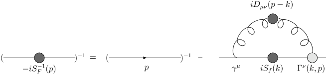
FIG. 1.: Diagrammatic representation of the Dyson-Schwinger equation for the inverse quark propagator $S^{-1}(p)$.

FIG. 2.: Solutions to the massless quark DSE with the Curtis-Pennington vertex and Cudell-Ross gluon propagator at the couplings $\alpha=0.2,0.6,1.0,1.4$. The critical value in this scheme was found to be $\alpha_{c}\approx 1.45$.

FIG. 3.: The wavefunction $F$ with an explicit quark mass, $m(\mu)=0.2$ for sub- and super-critical values of the coupling $\alpha$.

FIG. 4.: Mass function $M(p)$ with an explicit current quark mass, $m(\mu)=0.2$.

FIG. 5.: Estimated variation of $F(0),F(10^{6}),M(0)$ and $M(10^{6})$ due to a finite UV cutoff, as a function of the coupling. Error bars represent $\pm 1$ standard deviation.

FIG. 6.: Dynamically generated quark mass function, i.e. with $m(\mu)=0$, for couplings above critical, showing strongly damped oscillations.

FIG. 7.: Variation of $Z_{2}(\mu,\Lambda)m_{0}(\Lambda)$ with the UV cutoff $\Lambda$. The dashed line is a fit to the predicted $\ln\ln\Lambda$ dependence.

REFERENCES

- [1] C.D. Roberts and A.G. Williams, Prog. Part. Nucl. Phys. 33, 477-575 (1994), hep-ph/9403224.
- [2] A. Bashir and M.R. Pennington, Phys. Rev. D50, 7679-7689 (1994), hep-ph/9407350.
- [3] D.C. Curtis and M.R. Pennington, Phys. Rev. D42, 4165-4169 (1990).
- [4] J.S. Ball and T-W. Chiu, Phys. Rev. D22, 2542-2549 (1980).
- [5] F.T. Hawes and A.G. Williams, Phys. Rev. D51, 3081-3089 (1995), hep-ph/9410286.
- [6] P. Marenzoni, G. Martinelli, N. Stella and M. Testa, Phys. Lett. B318, 511-516 (1993).
- [7] A. Bashir “Chiral Symmetry Breaking for Fundamental Fermions” in Proceedings of the NATO ASI “Frontiers in Particle Physics: Cargèse 1994” (1995), hep-ph/9410399.
- [8] F.T. Hawes, A.G. Williams and C.D. Roberts, Phys. Rev. D54, 5361 (1996), hep-ph/9604402.
- [9] J-R. Cudell, A.J. Gentles and D.A. Ross, Nucl. Phys. B440, 525 (1995), hep-ph/9407220.
- [10] W.J. Schoenmaker, Nucl. Phys. B194, 535 (1982).
- [11] J.S. Ball, M. Baker and F. Zachariasen, Nucl. Phys. B186, 531 (1981); J.S. Ball, M. Baker and F. Zachariasen, Nucl. Phys. B186, 560 (1981).
- [12] P.V. Landshoff and O. Nachtmann, Z. Phys C35, 405 (1987);
- [13] See for example A. Donnachie and P.V. Landshoff, Phys. Lett. B185, 403 (1987); A. Donnachie and P.V. Landshoff, Nucl. Phys. B311, 509 (1989); J-R. Cudell, A. Donnachie and P.V. Landshoff, Nucl. Phys. B322, 55 (1989).
- [14] J-R. Cudell and D.A. Ross, Nucl. Phys. B359 247-261 (1991).
- [15] See for example D.C. Curtis and M.R. Pennington, Phys. Rev. D48, 4933-4939 (1993).
- [16] M.J.D. Powell, in P. Rabinowitz (ed.) Numerical Methods for Nonlinear Algebraic Equations, Gordon and Breach (1970).
- [17] J.M. Cornwall, R. Jackiw and E. Tomboulis, Phys. Rev. D10, 2428-2445 (1974).
- [18] K. Buttner and M.R. Pennington, Phys. Rev. D52 5220-5228 (1995), hep-ph/9506314.
- [19] F.T. Hawes, C.D. Roberts and A.G. Williams, Phys. Rev. D49 4683-4693 (1994), hep-ph/9309263.