MZ-TH/96-39
hep-ph/9611378
Introduction to XLOOPS

Abstract

The program package XLOOPS calculates massive one- and two-loop Feynman diagrams. It consists of five parts:

• a graphical user interface

• routines for generating diagrams from particle input

• procedures for calculating one-loop integrals both analytically and numerically

• routines for massive two-loop integrals

• programs for numerical integration of two-loop diagrams.

The package relies on the application of parallel space techniques. The treatment of tensor structure and the separation of UV and IR divergences in analytic expressions is described in this scheme. All analytic calculations are performed with MAPLE. Two-loop examples taken from Standard Model calculations are presented. The method has recently been extended to all two-loop vertex topologies, including the crossed topology, graphs with divergent subloops and IR divergent diagrams. This will be included in the XLOOPS package in the near future.

1
XLOOPS – an introduction
to parallel space techniques
Dirk Kreimer

The package XLOOPS presented in this workshop relies on the application of parallel space techniques. We introduce these techniques covering the following topics:

• The generation of integral representations for massive two-loop diagrams.

• The treatment of tensor structures.

• The handling of the $\gamma$-algebra in this scheme.

• The separation of UV and IR divergences in analytic expressions.

We present two-loop examples taken from Standard Model calculations.

1.1 Introduction

In last year’s conference in Pisa, AIHENP95, David Broadhurst and myself presented for the first time results concerning a fascinating connection between knot theory and Feynman diagrams.¹ Meanwhile this has lead to numerous results in field theory, as well as in knot theory and number theory.² We are still working in that area, and the results are even more intriguing, with the connection between transcendental numbers arising in counterterms and knots associated with the Feynman graphs becoming more and more specific. David Broadhurst and I just finished a joint two month stay at the University of Tasmania, where Bob Delbourgo invited us to continue our collaboration on the subject. As a consequence, David had to go back to teach at summer schools directly after our stay in Tasmania, so that for him it is not possible to attend this conference.

Today, I would like to focus on the techniques used in the package XLOOPS presented at this workshop. It is based on a very simple idea: that it might be useful to combine dimensional regularization with the fact that each Green function offers a distinguished subspace of spacetime - the space spanned by all its external momenta. This very fact was used as a convenient means to define dimensional regularization, for example in Collins text book.³

Amazingly, a systematic exploration of this idea allows to make progress for the calculation of general massive one- and two-loop Green function. The package, as it is presented in this conference, focuses on two- and three-point Green functions.⁴ While Lars Brücher and Johannes Franzkowski will report on the package XLOOPS itself, Alexander Frink will report on progress for the scalar two-loop three-point functions, covering planar and non-planar topologies, results which were already used in recent Standard Model calculations.⁵

1.2 Parallel and Orthogonal Spaces

In our approach, we use the fact that any non-trivial Green function furnishes a set of external momenta, on which it depends. A $n$-point Green functions provides in fact $n-1$ independent external momenta $p_{i}$. This allows to write any loop momentum $k_{i}$ as a sum of two covariant vectors, $k_{i}^{\mu}=k_{i,\parallel}^{\mu}+k_{i,\perp}^{\mu}$, where $k_{i,\parallel}$ has components in a space which is the linear span of the external momenta $p_{i}$, the parallel space, while $k_{i,\perp}$ is in its orthogonal complement, $\sum_{\mu}k_{i,\perp}^{\mu}p_{i\mu}=0$. Dimensional continuation happens in the orthogonal space.

1.2.1 Two-point functions

To consider the first specific example, we turn to a massive one-loop two-point function, providing a scalar integral of the form

$$I_{2}:=\int d^{D}\!k\;\frac{1}{[k^{2}-m_{1}^{2}][(k+q)^{2}-m_{2}^{2}]}\equiv\int\frac{d^{D}\!k}{P_{1}\,P_{2}}.$$ (1)

In parallel and orthogonal space variables, we have

$$I_{2} = \frac{2\pi^{\frac{D-1}{2}}}{\Gamma(\frac{D-1}{2})}\int_{-\infty}^{\infty}dk_{\parallel}\int_{0}^{\infty}dk_{\perp}\frac{k_{\perp}^{D-2}}{[k_{\parallel}^{2}-k_{\perp}^{2}-m_{1}^{2}][(k_{\parallel}+q)^{2}-k_{\perp}^{2}-m_{2}^{2}]}$$ (2)

$$= \frac{2\pi^{\frac{D-1}{2}}}{\Gamma(\frac{D-1}{2})}\int_{-\infty}^{\infty}dk_{\parallel}\frac{1}{P_{2}-P_{1}}\int_{0}^{\infty}dk_{\perp}\left[\frac{k_{\perp}^{D-2}}{P_{1}}-\frac{k_{\perp}^{D-2}}{P_{2}}\right],$$

where

$$k^{\mu}=k_{\parallel}e_{\parallel}^{\mu}+k_{\perp}^{\mu},\,\,e_{\parallel}^{\mu}=\frac{q^{\mu}}{\sqrt{q^{2}}},\,\,k_{\perp}\cdot q=0.$$ (3)

We straightforwardly integrate the orthogonal space to find expressions which involve

$$\left[P_{i}\mid_{k_{\perp}=0}\right]^{\frac{D-3}{2}},$$ (4)

which determine the cut structure of the result. Note that we avoid the Wick rotation and Feynman parametrizations altogether. The remaining integration with respect to $dk_{\parallel}$ can be done easily. For example, we can reinterprete it as an integral representation of a ${\cal R}$-function.⁶ Upon expanding in $D-4$, we recover the standard results of perturbation theory.

If we go to the two-loop level, we have five non-trivial integrations. We had two for the one-loop case, and for the two-loop case we have one more than twice this number, as there is an extra angular integration in orthogonal space, due to the presence of a non-trivial scalar product $l_{\perp}\cdot k_{\perp}$. It is known that straightforward application of the parallel space method gives a two-fold integral representation.⁷ This integral representation is the basis for the two-loop two-point package included in $XLOOPS$.

1.2.2 Three-point functions

Now we have a two-dimensional parallel space. Accordingly, in the one-loop case, the scalar one-loop integral has the following form in parallel and orthogonal space variables

$$I_{3} = \frac{2\pi^{\frac{D-2}{2}}}{\Gamma(\frac{D-2}{2})}\int_{-\infty}^{\infty}d\!k_{0}d\!k_{1}\frac{1}{[P_{i}-P_{j}][P_{i}-P_{k}]}\int_{0}^{\infty}d\!k_{\perp}\frac{k_{\perp}^{D-3}}{P_{i}}+\mbox{perm.~{}in $i,j,k$},$$

$$P_{1} = k_{0}^{2}-k_{1}^{2}-k_{\perp}^{2}-m_{1}^{2},$$

$$P_{2} = (k_{0}+q_{1,0})^{2}-(k_{1}+q_{1,1})^{2}-k_{\perp}^{2}-m_{2}^{2},$$

$$P_{3} = (k_{0}+q_{2,0})^{2}-(k_{1}+q_{2,1})^{2}-k_{\perp}^{2}-m_{3}^{2},$$ (5)

where

$$k_{\parallel}^{\mu}=k_{0}e_{1}^{\mu}+k_{1}e_{2}^{\mu},\,\,k^{\mu}=k_{\parallel}^{\mu}+k_{\perp}^{\mu},$$

$$e_{1}\cdot k_{\perp}=e_{2}\cdot k_{\perp}=0,\,span\{e_{1},e_{2}\}=span\{q_{1},q_{2}\}.$$ (6)

There are two non-trivial integrations for the parallel space, assumed to be spanned by two external momenta $q_{1},q_{2}$, and one for the modulus of $k_{\perp}$. One can proceed by explicitly using the signature of spacetime in the parallel space: a shift $k_{0}\to k_{0}+k_{1}$ renders all propagators linear in the variable $k_{1}$. The orthogonal space integration confronts us with a non-trivial cut structure: the integrand obtains a factor $[P_{i}\mid_{k_{\perp}=0}]^{\frac{D-4}{2}}$. Due to the shift in $k_{0}$, the cut is confined to a half plane in complex $k_{1}$ space, so that we can use the residue theorem for one of the parallel space integrations. The resulting expression can be identified as an integral representation of a $R$-function or, equivalently, of a hypergeometric.⁶

In the two-loop case, some of the features remain. We are now confronted with four integrations for the parallel space, and three for the orthogonal space. As in the two-point case, we do the angular integration in the orthogonal space, with respect to $z=\frac{l_{\perp}\cdot k_{\perp}}{\mid l_{\perp}\mid\!\mid k_{\perp}\mid}$, first. This results in a non-trivial cut structure, and the remaining integrations are determined by the demand that as many as possible can be done as residue integrals by closing the contour at infinity. A residue contributes only if it is located in the interior of the contour, and this results in constraints for the remaining variables. It turns out that these constraints determine the remaining domains of integrations to be finite triangles in the space of two remaining parallel space variables. At this level we are talking about a four-fold integral representation. Two further integrations in the orthogonal space variables $l_{\perp}^{2},k_{\perp}^{2}$ can be achieved for the planar topology, resulting in a two-fold integral representation, by using Euler transformations.⁸ Alexander Frink achieved a similar result for the non-planar topologies, which was already used and tested recently.⁵ He will report on these achievements in his talk in detail.

1.2.3 The general case

One could extend the method to four-point Green functions (and higher). We have not included this at this stage, but do not see any conceptual problems to do so if necessary.

1.3 Tensor Structures and $\gamma$-Algebra

One of the most interesting features of our approach is its treatment of the spin structure of Green functions. We altogether avoid the calculation of single tensor integrals (though this is possible in XLOOPS, to make contact with more conventional methods), but directly calculate the characteristic polynomials of a graph.⁹

1.3.1 Two-point functions

Again let us go back to a one-loop two-point function to understand the idea. Any Green function will deliver polynomial expressions in $k_{0},\,k_{\perp}^{2}$ for its numerator. They might come distributed over various form factors.⁹ To handle this situation, we also separate the Clifford algebra into two orthogonal sub-algebras, according to the splitting into parallel and orthogonal spaces. Using basic properties of Clifford algebras, it is then easy to determine the characteristic polynomials. A trivial one-loop example is provided by the self energy of a fermion, dressed with a massless vector boson in the Feynman gauge

$$\int dk_{\parallel}\,dk_{\perp}\frac{\gamma_{\mu}[k_{\parallel}\gamma_{\parallel}-\gamma_{\perp}\cdot k_{\perp}+m]\gamma^{\mu}}{[(k+q)^{2}][k^{2}-m^{2}]}\rightarrow\int dk_{\parallel}\,dk_{\perp}\frac{[(2-D)k_{\parallel}\gamma_{\parallel}+m{\bf 1}]}{[(k+q)^{2}][k^{2}-m^{2}]}.$$ (7)

We have two formfactors, one proportional to $\gamma_{\parallel}$, the other one proportional to ${\bf 1}$ in spin space. In parallel space, the only element of the $\gamma$-algebra is $\gamma_{\parallel}^{\nu}=q^{\nu}q^{\mu}\gamma_{\mu}/q^{2}=\gamma\cdot e$, while the Clifford algebra in orthogonal space is spanned by elements $\gamma_{\perp}^{\nu}$, with $q\cdot\gamma_{\perp}=0$ and $\{\gamma_{\parallel},\gamma_{\perp}\}=0$.⁹ In the above example we found two very simple characteristic polynomials for the two formfactors, $(2-D)k_{\parallel}$ and $m$.

Note that any polynomial expression in $k_{\parallel},\,k_{\perp}^{2}$ can be calculated by either reducing the expression to some basic scalar integrals, or to trivial massive tadpoles, by using the following rules

$$k_{\parallel} = \frac{P_{2}-P_{1}+[m_{2}^{2}-m_{1}^{2}-q^{2}]}{2\sqrt{q^{2}}},$$

$$k_{\perp}^{2} = k_{\parallel}^{2}-P_{1}-m_{1}^{2},$$

$$\int d^{D}k\frac{[k_{\perp}^{2}]^{r}}{P_{1}\,P_{2}} = \int d^{D+2r}\frac{1}{P_{1}\,P_{2}}.$$ (8)

Johannes Franzkowski will have further comments on the implementation of these ideas at the two loop level in his talk.

1.3.2 Three-point functions

Here we have the possibility to reduce polynomial expressions in the variables $k_{0},\,k_{1},\,k_{\perp}^{2}$ to either two-point functions, or to basic scalar three-point functions. Again, we achieve this by solving for the above variables in terms of propagators, masses and external momenta. These reductions are already implemented in XLOOPS in the one-loop case, and will be available at the two-loop case in the near future.

1.4 UV and IR Divergences

We usually do a termwise determination of the UV degree of divergence for our characteristic polynomials. We subtract massless integrals to achieve finite integral representations, carefully avoiding oversubtractions and thus avoiding the generation of spurious infrared singularities.⁹ A main feature of our approach is that the subtraction is done termwise in the characteristic polynomial. This avoids oversubtractions for the non-leading terms in the characteristic polynomials, while only the powercounting for the leading terms in the characteristic polynomial agrees with the powercounting for the graph itself.

At the moment, we gain first experience for the subtraction of IR singularities from our integral representations in collaboration with Jochem Fleischer in Bielefeld.

At the two-loop level, we calculate the UV divergences of a Feynman graph analytically, and generate well-defined code for numerical integrations.⁹

1.5 Conclusions

Let me list our main results as follows:

• XLOOPS calculates arbitrary graphs in the Standard Model for one-loop two- and three-point functions. After specifying a consistent particle content for a chosen topology, the user can choose to get an analytic or numeric result.

• At the two-loop level, XLOOPS returns an analytic result for the UV-divergent part of any two-point Standard Model graph, and automatically generates code for the remaining finite part of the whole graph.

• We have integral representations for all scalar two-loop three-point functions and will implement the two-loop three-point case in XLOOPS in the future.

2
XLOOPS – a package calculating
one- and two-loop diagrams
Lars Brücher

A program package for calculating massive one- and two-loop diagrams is introduced. It consists of five parts:

• a graphical user interface

• routines for generating diagrams from particle input

• procedures for calculating one-loop integrals both analytically and numerically

• routines for massive two-loop integrals

• programs for numerical integration of two-loop diagrams.

Here the graphical user interface and the text interface to Maple are presented.

2.1 Introduction

It is a well known fact, that high precision calculations of reactions between elementary particles cannot be done without the aid of computer programs, as the number of Feynman graphs can easily reach one hundred and exceed this as well. So there have been developed several different packages, each solving only one aspect or part of such calculations. More amazing is the fact that there is no package covering the whole procedure of calculating graphs. So someone starting such a high precision calculation is confronted with the fact, that he has to learn the syntax of several different programs. To overcome this problem, the development of XLOOPS, a program package covering all aspects of the calculation of Feynman graphs up to two-loop level was started. The following sections will discuss the structure of XLOOPS and introduce the graphical user interface (GUI), which makes XLOOPS an ‘easy-to-handle’ program package.

2.2 The general structure of XLOOPS

To avoid being tied to special computer systems or architectures, XLOOPS is designed to be as much portable as possible. Therefore

• Maple V[1, 2],

• TCL/Tk[3]and

• C++[4] for numerical integrations

were chosen as programming languages, as they are available for almost every computer architecture and all common operating systems, like Unix, Windows (3.1, 95 and NT) and VMS.

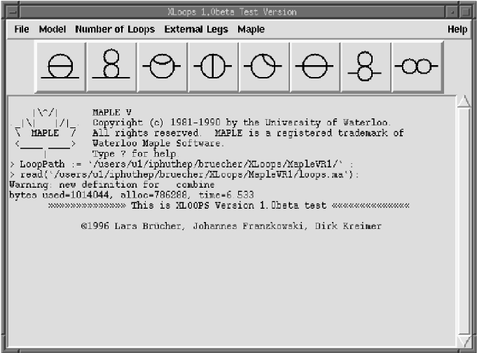
Figure 1: The main window of XLOOPS, which appears after starting the program

This choice of languages can also be seen as an indicator for the program structure of XLOOPS. As already mentioned in the abstract XLOOPS consist of

• a graphical user interface

• routines for generating diagrams from particle input

• procedures for calculating one-loop integrals both analytically and numerically

• routines for massive two-loop integrals

• programs for numerical integration of two-loop diagrams.

The graphical user interface should make the input of Feynman graphs as convenient as possible. This part is written in TCL/Tk and includes procedures for translating the user’s input into commands suitable for the following parts. These parts, the second, third and fourth part, are written in Maple V. They provide procedures which insert Feynman rules and evaluate loop-integrals analytically as far as possible. The user might also use these procedures without the graphical front end. The fifth part is the numerical integration program for the remaining integrals in two-loop calculations which is automatically invoked if needed. This part will be covered by the talks of J. Franzkowski and A. Frink.

When invoking XLOOPS the main window appears (see Fig. 1). It provides an overview of all topologies for a $n$-point $m$-loop function with $n$ and $m$ defined by the user in the main menu. By clicking on a topology the chosen graph appears in an extra window, suitable for inserting all virtual and non-virtual particles reacting (see Fig. 2). Having inserted the particles one can choose whether the program should evaluate the result expressed in loop-integrals by clicking on the ‘Evaluate’ button or if the program should return also the loop-integral evaluated in logarithms and dilogarithm by clicking on the ‘Evaluate Full’ button. The program itself starts now the calculation of the graph by giving an appropriate command to the Maple V part of the package, which actually gives back the analytical result displayed in the Maple output section of the main window. If a two-loop calculation is performed and all numerical values are given, the program also starts the numerical integration of the remaining integrals.

The result obtained by the evaluation can be saved or written out as a C program to a file. This is convenient for later use in a plotting program for example. For additional symbolic manipulations of the result, like inserting the renormalization conditions, a special window for direct Maple input exists. Moreover the program provides as additional features the possibility to insert the latest values from Particle Data Group[6] for the particle properties as a menu entry.

2.3 Examples calculated with XLOOPS

2.3.1 The decay $\bf H^{+}\longrightarrow W^{+}h^{0}$

To get more specific, the evaluation of $H^{+}\longrightarrow W^{+}h^{0}$ in the framework of the Two Higgs Doubletts Model[7] will be illustrated in this section. As an example we choose the top loop contribution to the self energy $H^{0}\rightarrow h^{0}$ necessary for the wave function renormalization and the triangle graph, which represents the actual one-loop correction (for a detailed discussion see [5]).

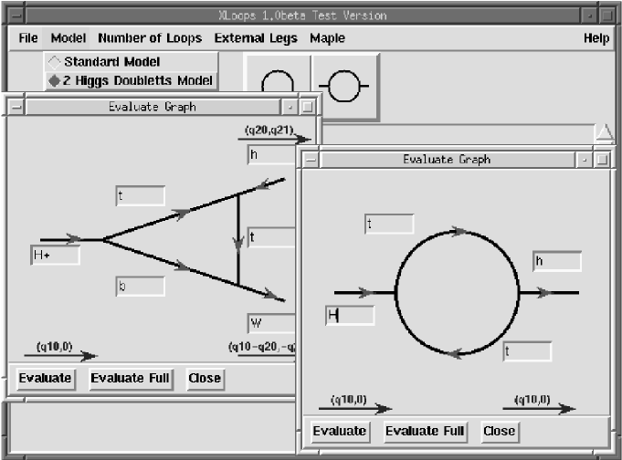
Figure 2: non-diagonal self energy graph and triangle graph contributing to $H^{+}\rightarrow W^{+}h^{0}$

After choosing the ‘2 Higgs Doubletts Model’ from the main menu and clicking on the graph we want to calculate, the window where the particles have to be inserted appears (see Fig. 2). When finished with typing in the particles and clicking on ‘Evaluate Full’ the following result for the $H^{0}\rightarrow h^{0}$ graph appears in the Maple output section:

G0 := [
            2     2                             2         2
           e  Mtop  sin(alpha) cos(alpha) I (q10  - 4 Mtop )
C1 = [1/32 -------------------------------------------------,
                             2   2          2   2
                      sin(tw)  Mw  sin(beta)  Pi

      2     2                                 2   2      2     2         2
1/64 e  Mtop  sin(alpha) cos(alpha) (2 Ln(4 Pi  MU ) I Pi  (q10  - 4 Mtop ) - 2

     2           2           2         2            2        2
   Pi  (- 2 I q10  + 6 I Mtop  + Pi q10  - 2 Pi Mtop  + I q10  gamma

          2                  2                 2                2        2
   + I q10  Ln(Pi) - 4 I Mtop  gamma - 4 I Mtop  Ln(Pi) - I Mtop  Ln(Mtop )

           2        2
   - I Mtop  Ln(Mtop  - I rho)

                                                     2                     2
   - I (%1 (Ln(1 - %1) - Ln(1 + %1) + I Pi) - Ln(Mtop  - I rho) - I Pi) q10

                                                       2                      2
   + 2 I (%1 (Ln(1 - %1) - Ln(1 + %1) + I Pi) - Ln(Mtop  - I rho) - I Pi) Mtop

       /         2   2          2   4
  ))  /  (sin(tw)  Mw  sin(beta)  Pi )
     /

],     C1]
                                          2
                                    - Mtop  + I rho
%1 :=                    Sqrt(1 + 4 ---------------)
                                             2
                                          q10

After evaluating the tadpole contribution in a similar way one can insert the on-shell condition, which in this case reads:

$$\delta Z_{H^{0}h^{0}}^{(1)}=\frac{1}{m_{h^{0}}^{2}-m_{H^{0}}^{2}}\Sigma_{H^{0}h^{0}}(m_{h^{0}}^{2})$$ (9)

This condition can be directly passed to Maple. In a similar manner the final result, after having summed up all graphs, can also be exported as C language code. This is very helpful for producing plots as shown in [5].

2.3.2 Flavour changing self-energy

As a second example the flavour changing self energy[8] from $s\rightarrow d$ in the framework of the Standard Model will be shown.

After having inserted the particle properties from the main menu entry and having attached the appropriate particle at each particle line as shown in Fig. 3 the evaluation is again started with ‘Evaluate Full’. In this case the program first starts the Maple part to evaluate the divergent part of the integral and the two-fold integral representation suitable for later numerical integration. As all numerical values are given, XLOOPS starts the remaining numerical integration. The result is displayed in the main window as a function of the form factors. Each of the form factors’ coefficients is displayed as a series in $D-4$.

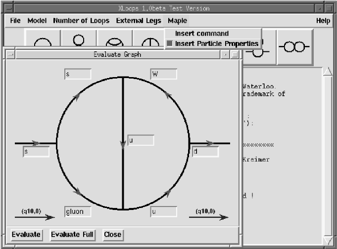
Figure 3: The self energy

2.4 Availability and Outlook

Currently a demo version of the program package, which does not include two-loop calculations, is available at

$$http://dipmza.physik.uni-mainz.de/\sim bruecher/xloops.html$$

where also additional information is accessible. The full version, which currently evaluates all one-loop graphs up to the 3-point function and all two-loop graphs up to the 2-point function, will also be accessible there, when it is fully tested. At the moment work to incorporate the 2-loop 3-point and the 1-loop 4-point function is in progress.

In future, procedures that automatically draw all Feynman graphs for a given process and display them in Postscript format should be added as well as procedures for automatic renormalization.

3
Automatic calculation of massive
two-loop self-energies with XLOOPS
Johannes Franzkowski

Within the program package XLOOPS it is possible to calculate self-energies up to the two-loop level for arbitrary massive particles. The program package – written in MAPLE [1, 2] – is designed to deal with the full tensor structure of the occurring integrals. This means that applications are not restricted to those cases where the reduction to scalars via equivalence theorem is allowed.

The algorithms handle two-loop integrals analytically if this is possible. For those topologies where no analytic result for the general mass case is available, the diagrams are reduced to integral representations which encounter at most a two-fold integration. These integral representations are numerically stable and can be performed easily using VEGAS [3, 4].

3.1 Structure of the XLOOPS package

The aim of XLOOPS is to provide the user with a program package for complete evaluation of Feynman diagrams. The package consists of the following parts:

• Input via Xwindows interface:
  In a window the user selects the topology which shall be calculated. A Feynman diagram pops up in which the particle names have to be inserted.

• Processing with MAPLE:
  The selected diagram is evaluated. The necessary steps for reducing the numerator – the so-called characteristic polynomial – are performed by routines written for MAPLE. The result is expressed in terms of one- and two-loop integrals.

• Evaluation of one-loop integrals:
  One-loop one-, two- and three-point integrals are calculated analytically or numerically to any tensor degree using MAPLE.

• Evaluation of two-loop integrals:
  All two-loop two-point topologies including tensor integrals are supported by the MAPLE routines. For those topologies where no analytic result is known, XLOOPS creates either an analytic two-fold integral representation or integrates numerically with the help of VEGAS using C++. The other topologies can be calculated analytically or numerically like the one-loop integrals.

In the remainder of this report the MAPLE routines, especially the treatment of two-loop integrals is described in detail.

3.2 The MAPLE part

3.2.1 Input

The user’s input is inserted conveniently by using the Xwindows interface – there is another contribution by L. Brücher which describes this interface in more detail – but it can also be typed in directly in a MAPLE session if the conventions of the manual [5] are respected.

In any case the XLOOPS routines expect as input either a Feynman diagram or a single integral. In XLOOPS code Feynman diagrams look like
         EvalGraph1(3,[bottom,charmbar,wp,bottombar,gluon,
                               gluon,charm,charmbar,bottom]);
         EvalGraph2(6,[up,upbar,gluon,upbar,up,gluon,
                               gluon,up,upbar,up,upbar,gluon]);
EvalGraph1 calculates one-loop, EvalGraph2 two-loop diagrams. The first argument denotes the number of the topology, the second is the list of particles. Single integrals have the following notation:
         OneLoop3Pt($p_{0},p_{1},p_{2}$,q10,q20,q21,m1,m2,m3);
         TwoLoop2Pt2($p_{0},p_{1},r_{0},r_{1},s$,q10,m1,m2,m3,m4,m5);
The $p_{i},r_{i},s$ determine the tensor structure $l_{0}^{p_{0}}\,l_{1}^{p_{1}}\,l_{\perp}^{p_{2}}$ and $l_{0}^{p_{0}}\,l_{\perp}^{p_{1}}\,k_{0}^{r_{0}}\,k_{\perp}^{r_{1}}\,z^{s}$ respectively – in the notation of section 2.3. The other arguments describe momentum components and masses. A detailed list of all conventions will be given in the XLOOPS manual [5], the one-loop sector is also described separately [6].

3.2.2 Characteristic polynomial

In the case of a single integral XLOOPS skips the following steps. If a complete diagram has to be evaluated, the routines proceed as follows:

• The topology – that means the information how the internal lines are connected – is generated.

• The Feynman rules are inserted. At present XLOOPS knows all Feynman rules of the Standard model (electroweak and QCD) and its extension to two Higgs doublets. The incorporation of additional models is simple.

• The symmetry factor of the diagram is determined.

• The characteristic polynomial (the numerator of the diagram) is evaluated in terms of parallel and orthogonal space variables. For that purpose XLOOPS knows the rules for the SU(N) algebra and how to reduce strings of Dirac matrices. If necessary it takes the trace of the Dirac matrices.

• Finally the code is expressed in terms of one- and two-loop integrals.

3.2.3 Parallel and orthogonal space

The evaluation of the Dirac algebra as well as of the integrals simplifies if one makes use of the splitting of the momentum components in parallel and orthogonal space variables – see D. Kreimer’s contribution for details. The definition is simple: The parallel space describes the sub-space spanned by the external momenta, whereas the orthogonal space is the orthogonal complement of the parallel space.

In the two-point case only one external momentum is present. Therefore the parallel space is one-dimensional. The loop momenta $l$ and $k$ are written as

$$l_{0} = \frac{l\cdot q}{\sqrt{q^{2}}}\qquad\mbox{(projection in direction of $q$)}$$

$$l_{\bot} = \sqrt{l_{0}^{2}-l^{2}}\qquad\mbox{(the same decomposition holds for $k$)}$$

$$l^{2} = l_{0}^{2}-l_{\bot}^{2}$$

$$k^{2} = k_{0}^{2}-k_{\bot}^{2}$$

$$l\cdot k = l_{0}k_{0}-l_{\bot}k_{\bot}\cos\vartheta$$

The integration measure simplifies in the following sense:

• one-loop case:

  $$\int\!d^{D}l=\int\limits_{-\infty}^{\infty}\!\!dl_{0}\int\!d^{D-1}l_{\bot}=\frac{2\pi^{\frac{D-1}{2}}}{\Gamma(\frac{D-1}{2})}\,\int\limits_{-\infty}^{\infty}\!\!dl_{0}\int\limits_{0}^{\infty}dl_{\bot}\,l_{\bot}^{D-2}$$

  The $D$-dimensional integral reduces to two one-dimensional integrations.

• two-loop case:

  $$\int\!d^{D}l\,\int\!d^{D}k=\int\limits_{-\infty}^{\infty}\!\!dl_{0}\int\limits_{-\infty}^{\infty}\!\!dk_{0}\,\int\!d^{D-1}l_{\bot}\int\!d^{D-1}k_{\bot}$$

  $$= \frac{4\pi^{\frac{D-1}{2}}\pi^{\frac{D-2}{2}}}{\Gamma(\frac{D-1}{2})\Gamma(\frac{D-2}{2})}\int\limits_{-\infty}^{\infty}\!\!dl_{0}\int\limits_{-\infty}^{\infty}\!\!dk_{0}\,\int\limits_{0}^{\infty}dl_{\bot}\,l_{\bot}^{D-2}\int\limits_{0}^{\infty}dk_{\bot}\,k_{\bot}^{D-2}\int\limits_{0}^{\pi}d\vartheta\,\sin^{D-3}\vartheta$$

  The $2D$-dimensional integral is now replaced by five one-dimensional integrations.

3.3 Two-loop integrals

The aim of our two-loop routines is not only to solve special mass cases or kinematical regions. They also supply the general case where all internal masses are different and the external momenta can be completely arbitrary. Full tensor structure and not only the scalar case is supported. As a consequence these general routines cannot return analytic results for all topologies. Therefore we adopt the following strategy:

1. separate the divergent parts (in any case analytically calculable)

2. find a two-fold integral representation (in $D=4$)

3. integrate numerically the two-fold integral

In the following we comment these three items.

3.3.1 UV divergent integrals

For the separation of divergences it is necessary to find a convenient subtraction term. If a two-loop integral is multiplied by a term like the one in brackets

$$\int d^{D}ld^{D}k\,\,\,\frac{l_{\mu_{1}}\cdots l_{\mu_{n}}}{{\cal P}_{1}(l){\cal P}_{2}(l){\cal P}_{3}(l+k){\cal P}_{4}(k){\cal P}_{5}(k)}$$

$$\to \int d^{D}ld^{D}k\,\,\,\frac{l_{\mu_{1}}\cdots l_{\mu_{n}}}{{\cal P}_{1}(l){\cal P}_{2}(l){\cal P}_{3}(l+k){\cal P}_{4}(k){\cal P}_{5}(k)}\,\,\left(1-\frac{{\cal P}_{1}(l){\cal P}_{2}(l){\cal P}_{3}(l+k)}{l^{4}(l+k)^{2}}\right)^{m}$$

it can be shown that the degree of divergence is decreased by $m$ steps [7]. To be specific, in the case of a logarithmic divergent integral which corresponds to the case $m=1$ one gets a difference of two terms which turns out to be convergent. To recover the original integral it is necessary to add the subtraction term again.

$$\underbrace{\int d^{D}ld^{D}k\,\,\,\frac{l_{\mu}l_{\nu}}{{\cal P}_{1}(l){\cal P}_{2}(l){\cal P}_{3}(l+k){\cal P}_{4}(k){\cal P}_{5}(k)}-\int d^{D}ld^{D}k\,\,\,\frac{l_{\mu}l_{\nu}}{l^{4}(l+k)^{2}{\cal P}_{4}(k){\cal P}_{5}(k)}}_{\mathrm{convergent}}$$

$$+\underbrace{\int d^{D}ld^{D}k\,\,\,\frac{l_{\mu}l_{\nu}}{l^{4}(l+k)^{2}{\cal P}_{4}(k){\cal P}_{5}(k)}}_{\mathrm{divergent}}$$

The first line which denotes the convergent part is treated in $D=4$ and will be reduced to a two-fold integral representation which is solved numerically. The second line contains the divergent part which can be solved analytically in $D\not=4$.

3.3.2 Integration strategy

We integrate directly in momentum space. With the splitting in parallel and orthogonal space variables one gets for two-point functions:

$$\int d^{4}l\int d^{4}k=8\pi^{2}\!\!\!\!\underbrace{\int\limits_{-\infty}^{\infty}\!\!\!dl_{0}dk_{0}}_{\mathrm{numerically}}\underbrace{\int\limits_{0}^{\infty}\!\!l_{\perp}^{2}dl_{\perp}k_{\perp}^{2}dk_{\perp}\int\limits_{0}^{\pi}\!\!\sin\vartheta d\vartheta}_{\mathrm{analytically}}$$

The $l_{0}$ and $k_{0}$ integrations are left for numerical evaluation. All other integrations are performed analytically.

Up to now we solved all two-point topologies for scalar and tensor evaluations. In the three-point case all topologies are solved for the scalar case. This will be subject of the contribution by A. Frink. At present our methods are applied to the three-point tensor and the four-point scalar integrals.

In the following we concentrate on the two-point topologies:

The worst case is of course the master topology [8]:

$$\int d^{4}l\int d^{4}k\,\,\frac{l_{0}^{a}\,l_{\perp}^{b}\,k_{0}^{c}\,k_{\perp}^{d}}{{\cal P}_{1}\cdots{\cal P}_{5}}$$

$$= 8\pi^{2}\int\limits_{-\infty}^{\infty}dl_{0}\int\limits_{-\infty}^{\infty}dk_{0}\int\limits_{0}^{\infty}dl_{\bot}\int\limits_{0}^{\infty}dk_{\bot}\int\limits_{0}^{\pi}d\vartheta\,\,\,\frac{l_{0}^{a}\,l_{\bot}^{b+2}\,k_{0}^{c}\,k_{\bot}^{d+2}\sin\vartheta}{{\cal P}_{1}\cdots{\cal P}_{5}}$$

$${\cal P}_{1} = l_{0}^{2}-l_{\bot}^{2}-m_{1}^{2}+i\varrho$$

$${\cal P}_{2} = (l_{0}+q)^{2}-l_{\bot}^{2}-m_{2}^{2}+i\varrho$$

$${\cal P}_{3} = (l_{0}+k_{0})^{2}-l_{\bot}^{2}-k_{\bot}^{2}-2l_{\bot}k_{\bot}\cos\vartheta-m_{3}^{2}+i\varrho$$

$${\cal P}_{4} = (k_{0}-q)^{2}-k_{\bot}^{2}-m_{4}^{2}+i\varrho$$

$${\cal P}_{5} = k_{0}^{2}-k_{\bot}^{2}-m_{5}^{2}+i\varrho$$

The angular integration is elementary. For the orthogonal space integration the residue theorem is applied twice. The analytic result then is the following two-fold integral representation (written for the scalar case in dimensionless variables $x,y$).

$$\int\limits_{-\infty}^{\infty}dx\int\limits_{-\infty}^{\infty}dy\,\,\frac{\log(w_{3}+w_{2}+w_{5})+\{\mbox{similar terms}\}}{(w_{1}^{2}-w_{2}^{2})(w_{4}^{2}-w_{5}^{2})}$$

$$w_{1} = \sqrt{x^{2}-\frac{m_{1}^{2}-i\varrho}{q^{2}}}$$

$$w_{2} = \sqrt{(x+1)^{2}-\frac{m_{2}^{2}-i\varrho}{q^{2}}}$$

$$w_{3} = \sqrt{(x+y)^{2}-\frac{m_{3}^{2}-i\varrho}{q^{2}}}$$

$$w_{4} = \sqrt{(y-1)^{2}-\frac{m_{4}^{2}-i\varrho}{q^{2}}}$$

$$w_{5} = \sqrt{y^{2}-\frac{m_{5}^{2}-i\varrho}{q^{2}}}$$

3.3.3 Numerical evaluation

The two-fold integral representation can be directly taken for numerical evaluation. We compared the results with available data. The data coincide perfectly with results from Shimizu, Kato and Fujimoto [9]. They were also verified in several asymptotic limits [10, 11].

3.4 Future extensions

The XLOOPS package is at present far from being saturated. The most important extension will be the incorporation of two-loop three-point (and four-point) functions. In addition a drawing routine for diagrams (generating Postscript output) will also be included as well as the possibility of evaluating complete processes and the option to renormalize the processes automatically.

4
Massive two-loop vertex functions
Alexander Frink

Calculating massive two-loop vertex functions by splitting integrations into parallel and orthogonal space components has been demonstrated to give a convenient twofold integral representation suitable for numerical evaluation. This method is now extended to more topologies, including the crossed topology, graphs with divergent subloops and infrared divergent diagrams. The connection between this representation and physical and anomalous thresholds is examined.

4.1 The crossed vertex function

The scalar crossed vertex function (Fig. 4a) can be calculated similarly to the planar vertex function (Fig. 4b) with the orthogonal/parallel space integration technique presented in [1]. The volume element is written as $d^{4}l\,d^{4}k=\frac{1}{2}dl_{0}\,dk_{0}\,dl_{1}\,dk_{1}\,ds\,dt\,d\alpha\,dz/\sqrt{1-z^{2}}$, where $l_{0}$, $l_{1}$, $k_{0}$ and $k_{1}$ are the components of the loop momenta parallel to the external momenta, $s\equiv l_{\perp}^{2}$, $t\equiv k_{\perp}^{2}$ and $z$ is the cosine of the angle between $\vec{l}_{\perp}$ and $\vec{k}_{\perp}$. The procedure can be divided into the following main steps:

Figure 4: Topologies covered in this article

• linearization of propagators in $l_{1}$ and $k_{1}$ by shifting $l_{0}\to l_{0}+l_{1}$, $k_{0}\to k_{0}+k_{1}$

• integration over orthogonal space angles ($\alpha$ and $z$)

• integration over $l_{1}$ and $k_{1}$ with Cauchy’s theorem, avoiding cuts resulting from the $z$ integration

• integration over $s$ and $t$ with Euler’s change of variables

• numerical evaluation of the remaining integrations over $l_{0}$ and $k_{0}$ in a finite region

The main complication arises here as both loop momenta $l$ and $k$ have to flow through two propagators in common. To perform the $z$ integration as in [1], we have to apply a partial fraction decomposition in these two propagators, in order that in the difference term the $z$ dependence drops out. Each term of the partial fraction decomposition can be calculated separately and similarly to the planar vertex function as in [1], however the condition in which way to close the contour for the $l_{1}$ and $k_{1}$ residue integrations is different for both terms: $l_{0}+k_{0}-e_{1}{\raisebox{-1.72218pt}[0.0pt][0.0pt]{$<$}\atop\raisebox{0.90417pt}[0.0pt][0.0pt]{$>$}}0$ and $l_{0}+k_{0}+e_{2}{\raisebox{-1.72218pt}[0.0pt][0.0pt]{$<$}\atop\raisebox{0.90417pt}[0.0pt][0.0pt]{$>$}}0$ resp., where $e_{1}$ and $e_{2}$ are components of the external momenta. As a consequence poles from the difference term which lie on the real axis also have to be taken into account. These poles give rise to several unbounded areas in the $(l_{0},k_{0})$ plane in addition to triangles. Nevertheless these add up to zero outside the finite region shown in Fig. 5.

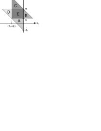
Figure 5: Effective integration region in the $(l_{0},k_{0})$ plane for the crossed vertex function

After the residue integrations we have the intermediate result

$$V_{C} = \sum_{j=1}^{10}\int\!\!\!\int\limits_{\!\!A_{j}}\!dl_{0}\,dk_{0}\int\limits_{0}^{\infty}\!ds\int\limits_{0}^{\infty}\!dt\,C_{j}\,\frac{1}{\tilde{a}_{1j}t+\tilde{b}_{1j}+\tilde{c}_{1j}c}\frac{1}{\tilde{a}_{2j}t+\tilde{b}_{2j}+\tilde{c}_{2j}c}$$ (10)

$$\hskip 28.45274pt\frac{1}{\tilde{a}_{3j}t+\tilde{b}_{3j}+\tilde{c}_{3j}c}\frac{1}{\sqrt{(a_{j}t+b_{j}+c_{j}s)^{2}-4st}}\,,$$

where $C_{j}$, $\tilde{a}_{kj}$, $\tilde{b}_{kj}$, $\tilde{c}_{kj}$, $a_{j}$, $b_{j}$ and $c_{j}$ are rational functions of $l_{0}$ and $k_{0}$, and $A_{j}$ is a subset of the area in Fig. 5. Some of the $\tilde{a}_{kj}$ and $\tilde{c}_{kj}$ vanish. Euler’s change of variables for $s$ and $t$ reduces the problem to integrals of the forms $\int\ln(x^{2}+rx+s)/(x^{2}+px+q)\,dx$ and $\int\arctan(x+a)/(x^{2}+px+q)\,dx$, which can be expressed in terms of dilogarithms and Clausen functions. Further details can be found in [2].

As for the planar vertex function a correlation between the various coefficients in Eq. (10) and physical thresholds resulting in an imaginary part of the diagram can be found: if an $\tilde{a}_{kj}$ or $\tilde{c}_{kj}$ is zero, then the accompanying $\tilde{b}_{kj}$ corresponds to a two-particle cut. The coefficients $b_{j}$ correspond either to three-particle cuts or the two-particle cut $q^{2}>(m_{1}+m_{2})^{2}$ which is somewhat hidden due to the partial fraction decomposition.

4.2 Anomalous Thresholds

The connection between the coefficients in our two-loop three-point representation and physical thresholds has been pointed out in [1] for the planar and above for the crossed topology. Now it will be demonstrated that anomalous thresholds are also accounted for correctly in this representation. As an example, let us consider the one-loop three-point function in Fig. 4c. By searching for solutions of the Landau equations [3], one can find a singularity which corresponds to no physical threshold at $1+2\mu_{1}\mu_{2}\mu_{3}-\mu_{1}^{2}-\mu_{2}^{2}-\mu_{3}^{2}=0$ where $\mu_{j}=(m_{1}^{2}+m_{2}^{2}+m_{3}^{2}-m_{j}^{2}-p_{j}^{2})m_{j}/(2m_{1}m_{2}m_{3})$. If we arbitrarily choose all masses equal, $m_{1}=m_{2}=m_{3}=1$, and $p_{1}^{2}=6$, $p_{2}^{2}=5$, these equations are fulfilled for $p_{3}^{2}=-4-\sqrt{15}\approx-7.873$. A plot of the real and imaginary part of this diagram for different values of $p_{3}^{2}$ in the vicinity of this point is shown in Fig. 6(left).

Let us now turn to the two-loop example Fig. 4d. The Landau equations give us a singularity for this graph at the same values as above for arbitrary $m_{4}$, $m_{5}$ and $m_{6}$. We recall the four-fold integral representation for the planar graph [1]:

$$V_{P}=\sum\limits_{j=1}^{4}\int\!\!\!\int\limits_{\!\!T_{j}}\!dl_{0}\,dk_{0}\,C\int\limits_{0}^{\infty}\frac{dt}{(t+t_{0})(t+t_{0}^{\prime})}\int\limits_{0}^{\infty}\frac{ds}{s+s_{0}}\frac{1}{\sqrt{(at+b+cs)^{2}-4st}}$$ (11)

$t_{0}$ and $t_{0}^{\prime}$ are quadratic functions in $k_{0}$. As was pointed out in [1], real roots of $t_{0}$ and $t_{0}^{\prime}$ inside the integration triangle correspond to physical thresholds $p_{1}^{2}>(m_{2}+m_{3})^{2}$ and $p_{2}^{2}>(m_{3}+m_{1})^{2}$ respectively. These conditions are fulfilled here. Let us denote the roots of $t_{0}$ and $t_{0}^{\prime}$ as $k_{0}^{(1,2)}$ and ${k_{0}^{(1,2)}}{{}^{\prime}}$ resp. Then it can be shown that below the anomalous threshold $k_{0}^{(2)}<k_{0}^{(1)}{}^{\prime}$ and above $k_{0}^{(2)}>k_{0}^{(1)}{}^{\prime}$. However, for the numerical integration over $l_{0}$ and $k_{0}$ (after partial fraction decomposition) the program only has to make a distinction between $t_{0}^{(\prime)}>0$ (real part only) and $t_{0}^{(\prime)}<0$ (additional imaginary part). Merely numerical stability gets slightly worse in the direct vicinity of the threshold. Fig. 6(right) shows the expected plot of real and imaginary parts.

Figure 6: Plot of real and imaginary parts of a vertex function in the vicinity of an anomalous threshold, one-loop (left) and two-loop (right)

4.3 Divergent diagrams

The method for calculating massive two-loop vertex functions by splitting integrations into parallel and orthogonal space components works without modifications only for convergent integrals. The complication stems from the non-elementary integration over the cosine of the angle between $\vec{l}_{\perp}$ and $\vec{k}_{\perp}$, $z$, in $D=4-2\varepsilon$ dimensions

$$\int\limits_{-1}^{1}\frac{1}{\sqrt{1-z^{2}}}\frac{1}{A+Bz+i\eta}\,dz\longrightarrow\int\limits_{-1}^{1}(1-z^{2})^{\frac{D-5}{2}}\frac{1}{A+Bz+i\eta}\,dz\,,$$ (12)

which can only be expressed in terms of hypergeometric functions instead of a simple square root.

In order to avoid this, one has to subtract a simpler function with the same structure of divergence. The difference is finite and can be calculated with the parallel/orthogonal space technique in four dimensions, whereas the subtracted function should be calculable in $D$ dimensions. A first example for an UV divergent scalar vertex function at zero momentum transfer has been given in [4]. This will now be extended to other genuine vertex topologies as well as infrared divergent diagrams.

4.3.1 Infrared divergences

As an example let us consider the planar graph depicted in Fig. 4b with $q_{1}^{2}=m_{4}^{2}$, $q_{2}^{2}=m_{5}^{2}$ and $m_{6}\to 0$. We choose the loop momentum $l$ to flow through $P_{1}\dots P_{3}$ and $k$ through $P_{4}\dots P_{6}$. This graph exhibits an infrared divergence for $k\to 0$. By subtracting the same diagram, but with $P_{3}$ replaced with $\tilde{P}_{3}=P_{3}\big{|}_{k=0}$, power-counting for small $k$ is improved by one unit, so the difference is now finite and can be calculated in four dimensions:

$$V_{IR} = \int\!d^{4}l\,d^{4}k\,\frac{1}{P_{1}P_{2}}\left(\frac{1}{P_{3}}-\frac{1}{\tilde{P}_{3}}\right)\frac{1}{P_{4}P_{5}P_{6}}$$ (13)

$$+\int\!d^{D}l\,\frac{1}{P_{1}P_{2}\tilde{P}_{3}}\int\!d^{D}k\,\frac{1}{P_{4}P_{5}P_{6}}+{\cal O}(\varepsilon)\,.$$

This involves the same main steps as for the crossed vertex function (see above). Since infrared divergences are endpoint singularities, all steps can be applied individually to both parts of the integrand, and the infrared divergence will not show until the last numerical integration over $k_{0}$ near $k_{0}\to 0$. But there the subtraction guarantees a well-defined limit.

Let us now demonstrate the integration steps for the subtracted term. The $z$ integration is trivial, since none of the propagators depends on $z$. Therefore there is no cut in the integrand which has to be avoided during the residue integrations. We have the freedom to close the contours analogously to the original term [1], i.e. for $l_{0}+k_{0}>0$ in the upper and for $l_{0}+k_{0}<0$ in the lower half plane. Then the integrations over $l_{1}$ and $k_{1}$ give conditions of the form $l_{0}{\raisebox{-1.72218pt}[0.0pt][0.0pt]{$<$}\atop\raisebox{0.90417pt}[0.0pt][0.0pt]{$>$}}x$ and $k_{0}{\raisebox{-1.72218pt}[0.0pt][0.0pt]{$<$}\atop\raisebox{0.90417pt}[0.0pt][0.0pt]{$>$}}y$ for the individual propagators to contribute, which results in triangular regions listed in Table 1. The overlap of these triangles coincides with the overlap of the triangles from [1].

Table 1: Non-vanishing triangles from the subtracted term

propagators	conditions
$(P_{1},P_{5})$	$l_{0}+k_{0}<0$	$l_{0}+e_{1}-q_{z}>0$	$k_{0}+e_{2}+q_{z}>0$
$(P_{1},P_{6})$	$l_{0}+k_{0}<0$	$l_{0}+e_{1}-q_{z}>0$	$k_{0}>0$
$(P_{2},P_{4})$	$l_{0}+k_{0}>0$	$l_{0}-e_{2}-q_{z}<0$	$k_{0}-e_{1}+q_{z}<0$
$(P_{2},P_{6})$	$l_{0}+k_{0}>0$	$l_{0}-e_{2}-q_{z}<0$	$k_{0}<0$
$(P_{3},P_{4})$	$l_{0}+k_{0}>0$	$l_{0}<0$	$k_{0}-e_{1}+q_{z}<0$
$(P_{3},P_{5})$	$l_{0}+k_{0}<0$	$l_{0}>0$	$k_{0}+e_{2}+q_{z}>0$

The analytic evaluation of the subtracted part involves calculating one-loop three-point functions up to ${\cal O}(\varepsilon)$ [5]. This subtraction procedure is also applicable for small but non-zero $m_{6}$ in order to improve numerical stability and to extract the leading logarithm.

4.3.2 Graphs with divergent subloops

Ultraviolet divergent scalar diagrams as in Fig. 4e can also be calculated by subtracting an appropriate quantity with the same structure of divergence. This can be done by setting the masses in the inner subloop to zero. Let $k$ flow through the divergent subloop and $l$ in the outer loop. Defining $\tilde{P}_{4}=P_{4}\big{|}_{m_{4}=0}$ and $\tilde{P}_{5}=P_{5}\big{|}_{m_{5}=0}$, we have

$$V_{UV} = \int\!d^{4}l\,d^{4}k\frac{1}{P_{1}P_{2}P_{3}}\left(\frac{1}{P_{4}P_{5}}-\frac{1}{\tilde{P}_{4}\tilde{P}_{5}}\right)$$ (14)

$$+\int\!d^{D}l\int\!d^{D}k\frac{1}{P_{1}P_{2}P_{3}\tilde{P}_{4}\tilde{P}_{5}}+{\cal O}(\varepsilon)\,.$$

Performing the $z$, $l_{1}$ and $k_{1}$ integrations as above, we obtain the intermediate result

$$V_{UV,{\rm finite}} = \sum_{j=1}^{2}\int\!\!\!\int\!dl_{0}\,dk_{0}\int\limits_{0}^{\infty}\!ds\int\limits_{0}^{\infty}\!dt\,C\,\frac{1}{(s+s_{0})(s+s_{0}^{\prime})}$$ (15)

$$\hskip 28.45274pt\left(\frac{1}{\sqrt{(at+b+cs)^{2}-4st}}-\frac{1}{\sqrt{(at+\tilde{b}+cs)^{2}-4st}}\right)\,.$$

This can be readily expressed as a twofold integral representation over dilogarithms. The $l_{0}$ and $k_{0}$ integrations extend again over triangles. Note that the boundaries of the triangles depend solely on the external momenta and not on the internal masses.

The calculation of the subtracted part is done by first integrating the massless subloop in $k$, giving a result proportional to $(l^{2})^{-\varepsilon}$. The evaluation of the one-loop three-point function with non-integer powers of propagators can be done at least numerically.

The topology in Fig. 4f can be reduced to the topology in Fig. 4e by partial fraction decomposition in the propagators $P_{3}$ and $P_{6}$. Since the integration region in the $(l_{0},k_{0})$ plane is equal for both terms, they can be added again before integrating over $l_{0}$ and $k_{0}$. The case $m_{3}=m_{6}$ is handled by differentiating $V_{UV}$ with respect to $m_{3}$.

4.4 Outlook

Current work is done in the direct calculation of tensor integrals. A general method using subtraction terms similar to above has been proposed by D. Kreimer [6].

References

-
[1]
D.J. Broadhurst, D. Kreimer, Int.J.of Mod.Phys. C6, 519 (1995);
D. Kreimer, Phys.Lett. B354, 117 (1995);
D. Kreimer, Habilschrift: Renormalization and Knot Theory, to appear in Journal of Knot Theory and its Ramifications, preprint MZ-TH/96-18, q-alg/9607022, in print. -
[2]
D.J. Broadhurst, R. Delbourgo, D. Kreimer,
Phys.Lett. B366, 421 (1996);
D.J. Broadhurst, J.A. Gracey, D. Kreimer, Beyond the triangle and uniqueness relations: non-zeta terms at large from positive knots, to appear in Z.Phys.C, OUT-4102-46, MZ-TH/95-28, hep-th/9607174 (1996);
D.J. Broadhurst, On the enumeration of irreducible k-fold Euler sums and their roles in knot theory and field theory, to appear in J.Math.Phys., preprint OUT-4102-62, hep-th/9604128 (1996);
D.J. Broadhurst, D. Kreimer, Association of multiple zeta values with positive knots via Feynman diagrams up to 9 loops, preprint UTAS-PHYS-96-44 (1996), hep-th/9609128. - [3] J. Collins, Renormalization (Cambridge UP 1984).
-
[4]
L. Brücher, contributed paper at this conference;
J. Franzkowski, contributed paper at this conference;
A. Frink, contributed paper at this conference. - [5] A. Frink, B.A. Kniehl, D. Kreimer, K. Riesselmann, Heavy-Higgs Lifetime at Two Loops, Phys.Rev.D54 (1996) 4548; hep-ph/9606310.
-
[6]
D. Kreimer, Z. Phys. C54, 667 (1992);
D. Kreimer, Int. J. of Mod. Phys. A8, No.10, 1797, (1993);
L. Brücher, J. Franzkowski, D. Kreimer, Mod. Phys. Lett. A9, 2335 (1994);
L. Brücher, J. Franzkowski, D. Kreimer, Comp. Phys. Comm. 85, 153 (1995). - [7] D. Kreimer, Phys. Lett. B273, 277, (1991).
- [8] A. Czarnecki, U. Kilian, D. Kreimer, Nucl. Phys. B433, 259 (1995).
-
[9]
D. Kreimer, Mod.Phys.Lett. A9 (1994) 1105;
D. Kreimer, U. Kilian, K. Schilcher, Calculation of the flavour changing wave-function renormalization to , preprint MZ-TH/96-19 (1996).
2

References

-
[1]
B. W. Char, K. O. Geddes, G. H. Gonnet, B. L. Leong,
M. B. Monagan, S. M. Watt
Maple V Language Reference Manual, Springer (1991) -
[2]
B. W. Char, K. O. Geddes, G. H. Gonnet, B. L. Leong,
M. B. Monagan, S. M. Watt
Maple V Library Reference Manual, Springer (1991) -
[3]
J. K. Ousterhout
Tcl und Tk – Entwicklung grafischer Benutzerschnittstellen für das XWindow-System, Addison-Wesley (1995) -
[4]
B. Stroustrup
The C++ Programming Language, Addison-Wesley (1991) -
[5]
R. Santos, A. Barroso, L. Brücher
Top quark loop corrections to the decay in the Two Higgs Doublet Model
hep-ph 9608376, to be publ. in Phys. Lett. B -
[6]
R.M. Barnett et al.,
Phys. Rev. D54, 1 (1996) -
[7]
J. Velhinho, R. Santos and A. Barroso,
Phys. Lett. B322, 213 (1994) -
[8]
J. Franzkowski, D. Kreimer, U. Kilian, K. Schilcher,
Calculation of the flavour changing wave-function renormalization to ,
preprint MZ-TH 96-19 (1996)
3

References

- [1] B. W. Char, K. O. Geddes, G. H. Gonnet, B. L. Leong, M. B. Monagan, S. M. Watt. Maple V Language Reference Manual. Springer (1991)
- [2] B. W. Char, K. O. Geddes, G. H. Gonnet, B. L. Leong, M. B. Monagan, S. M. Watt. Maple V Library Reference Manual. Springer (1991)
- [3] G. P. Lepage. J. Comp. Phys. 27 (1978) 192
- [4] G. P. Lepage. Cornell Univ. Preprint CLNS-80/447 (1980)
- [5] L. Brücher, J. Franzkowski. The XLOOPS manual. (in preparation)
- [6] L. Brücher, J. Franzkowski, D. Kreimer. Comp. Phys. Comm. 85 (1995) 153
- [7] D. Kreimer. Mod. Phys. Lett. A9 (1994) 1105
- [8] D. Kreimer. Phys. Lett. B273 (1991) 277
- [9] J. Fujimoto, Y. Shimizu, K. Kato. Private communication
- [10] A. I. Davydychev, V. A. Smirnov, J. B. Tausk. Nucl. Phys. B410 (1993) 325
- [11] A. I. Davydychev, J. B. Tausk. Nucl. Phys. B397 (1993) 123
4

References

- [1] A. Czarnecki, U. Kilian and D. Kreimer, Nucl. Phys. B433 (1995) 259.
-
[2]
A. Frink, U. Kilian and D. Kreimer,
Mainz preprint MZ-TH/96-30,
hep-ph/9610285. - [3] L.D. Landau, Nucl. Phys. 13 (1959) 181.
- [4] A. Czarnecki, Karlsruhe preprint TTP 94-21, hep-ph/9410332.
- [5] U. Nierste, D. Müller and M. Böhm, Z. Phys. C57 (1993) 605.
- [6] D. Kreimer, Mod. Phys. Lett. A9 (1994) 1105.