Abstract

These notes contain some of the material I presented at TASI 96 on the comparison of the standard model with precision electroweak data. After a physical accounting of the dominant electroweak radiative corrections, including the effects of initial state bremsstrahlung, I examine how data from LEP and the SLC provides a clear test of the standard model. Apparent discrepancies in the $R_{b}$ and $R_{c}$ ratios, and their physical resolution, are also examined in some detail.

1 Introduction

Having to lecture on “Aspects of the Electroweak Theory” at TASI ’96, a school whose principal focus was on strings, duality and supersymmetry, presented a real challenge. Was there anything about the Standard Model, I asked myself, which would be both interesting and of use to the highly theoretical students attending TASI? In the end, I decided that perhaps two topics fit the bill: precision tests of the electroweak theory and fermion masses.

All students have heard the mantra that the standard model is firmly established by the amazing coincidence of its theoretical predictions with precision electroweak data, particularly that emanating from the $e^{+}e^{-}$ colliders operating at the $Z$ mass. Nevertheless, few students really have a feel for the difficulties involved in establishing this fact experimentally, or a good physical understanding for the theoretical basis for this agreement. For this reason, as a first topic of my lectures, I decided to talk in some detail about the physics lying behind the confrontation of precision data with the electroweak theory.

Strictly speaking fermion masses, on the other hand, lie beyond the standard model. That is, in the standard model, masses and mixing parameters are input quantities, not quantities which are determinable by theory. Nevertheless, it is clear that ultimately we want to arrive at a theory where these parameters are predictable. For this reason, it is interesting to discuss what we know at present about these quantities and understand to what extent this knowledge could eventually be “predicted” by a deeper theory. Thus, it seemed natural to make this the second topic of my lectures. In particular, since the origin of fermion masses probably is tied to physics at the Planck scale, a central question which I tried to answer in my lectures was what could be inferred from present data about the structure of lepton and quark mass matrices at the Planck scale. Because most of the material in the second part of my lectures is contained in my recent article with Wang[1], I have written up here only material from the first part of my lectures.

2 Confronting the Electroweak Theory with Experiment

The standard model of electroweak interactions is so well known by now[2] that I will only briefly sketch its principal elements, mostly to establish a common notation.

2.1 Elements of the Electroweak Theory

The Glashow-Salam-Weinberg electroweak theory is based on a $SU(2)\times U(1)$ gauge theory spontaneously broken to $U(1)_{\rm em}$. As a result of the symmetry breakdown, the $W^{\pm}$ and $Z$ gauge bosons acquire a mass. One gets the experimentally “correct” interrelation between the $W$ and $Z$ boson masses $[M^{o}_{W}=M^{o}_{Z}\cos\theta^{o}_{W}]$ if the agent causing the symmetry breakdown transforms as an $SU(2)$ doublet[3]. Furthermore, if this agent is a complex scalar doublet Higgs field (or fields) $\Phi$, then the Yukawa interactions of this field with fermions are a natural source for the fermion masses and mixing, after the symmetry breakdown.

The $SU(2)\times U(1)$ covariant Higgs kinetic energy term

$${\cal{L}}_{\rm kin}=-(D_{\mu}\Phi)^{\dagger}(D^{\mu}\Phi)~{},$$ (1)

with

$$D^{\mu}\Phi=\left[\partial^{\mu}-ig_{o}\frac{\tau_{a}}{2}W_{a}^{\mu}-ig^{\prime}_{o}\left(-\frac{1}{2}\right)Y^{\mu}\right]\Phi~{},$$ (2)

is the source for the weak boson masses once one assumes that the Higgs field obtains a non-zero VEV:

$$\langle\Phi\rangle=\frac{v_{o}}{\sqrt{2}}\left(\begin{array}[]{c}1\\ 0\end{array}\right)~{}.$$ (3)

This VEV provides mass for the charged fields $W_{\pm}^{\mu}=\frac{1}{\sqrt{2}}(W_{1}^{\mu}\mp iW_{2}^{\mu})$ and the linear combination of neutral fields $g_{o}W_{3}^{\mu}-g_{o}^{\prime}Y^{\mu}$. Specifically, defining new fields $Z^{\mu}$ and $A^{\mu}$ by

$$\left(\begin{array}[]{c}Z^{\mu}\\ A^{\mu}\end{array}\right)=\left[\begin{array}[]{cc}\cos\theta_{W}^{o}&-\sin\theta_{W}^{o}\\ \sin\theta^{o}_{W}&\cos\theta_{W}^{o}\end{array}\right]\left(\begin{array}[]{c}W_{3}^{\mu}\\ Y^{\mu}\end{array}\right)~{},$$ (4)

where $\tan\theta_{W}^{o}=g^{\prime}_{o}/g_{o}$, a simple calculation shows that

$$M_{W}^{o}=\frac{1}{2}g_{o}v_{o}~{};~{}~{}~{}M_{Z}^{o}=\frac{M_{W}^{o}}{\cos\theta_{W}^{o}}~{};~{}~{}~{}M_{A}^{o}=0~{}.$$ (5)

The Higgs doublet $\Phi$ contains one physical component, the Higgs boson $H$ and, effectively, one can write

$$\Phi\equiv\frac{1}{\sqrt{2}}\left(\begin{array}[]{c}v_{o}+H\\ 0\end{array}\right)~{}.$$ (6)

The couplings of $H$ to the gauge fields are fixed by the $SU(2)\times U(1)$ symmetry, but its mass $M_{H}^{o}$ is arbitrary, being linked to the unknown Higgs self-interactions.

The interactions of fermions with the gauge fields are also totally specified by the transformation properties of the fermions under $SU(2)\times U(1)$. These interactions involve the $SU(2)$ and $U(1)$ currents of the fermions

$$J_{a}^{\mu}=\sum_{i}\bar{f}_{i}\gamma^{\mu}(t_{a})_{i}f_{i}~{};~{}~{}~{}J_{Y}^{\mu}=\sum_{i}\bar{f}_{i}\gamma^{\mu}y_{i}f_{i}~{},$$ (7)

where $((t_{a})_{i},~{}y_{i})$ are the relevant representation matrices for the $i^{\rm th}$ fermion, coupled to the corresponding gauge fields:

$${\cal{L}}_{\rm int}=g_{o}J_{a}^{\mu}W_{a\mu}+g^{\prime}_{o}J_{Y}^{\mu}Y_{\mu}~{}.$$ (8)

Using the Weinberg angle $\theta_{W}^{o}$ and the physical fields $(W^{\pm},Z,A)$ the above can be rewritten as

$${\cal{L}}_{\rm int} = g^{\prime}_{o}\cos\theta_{W}^{o}(J_{3}^{\mu}+J_{Y}^{\mu})A_{\mu}+\frac{g_{o}}{2\sqrt{2}}\{J_{-}^{\mu}W_{+\mu}+J_{+}^{\mu}W_{-\mu}\}$$ (9)

$$+ \frac{g_{o}}{2\cos\theta_{W}^{o}}\left[2(J_{3}^{\mu}-\sin^{2}\theta_{W}^{o}(J_{3}^{\mu}+J_{Y}^{\mu}))\right]Z_{\mu}~{}.$$

The above formula provides three physical identifications:

(i) One recognizes the electromagnetic current

$$J^{\mu}_{\rm em}=J^{\mu}_{3}+J^{\mu}_{Y}$$ (10)

from its coupling to the photon field $A_{\mu}$.

(ii) Similarly, the strength of this coupling identifies the electric charge $e_{o}$ as the combination

$$e_{o}=g^{\prime}_{o}\cos\theta_{W}^{o}=g_{o}\sin\theta_{W}^{o}~{}.$$ (11)

(iii) Finally, one identifies a neutral current

$$J^{\mu}_{\rm NC}=2(J^{\mu}_{3}-\sin^{2}\theta^{o}_{W}J^{\mu}_{\rm em})$$ (12)

as the current which couples to the $Z_{\mu}$ boson.

Using as parameters $e_{o}$ and $\sin\theta_{W}^{o}$ one can write

$${\cal{L}}_{\rm int}=e_{o}J^{\mu}_{\rm em}A_{\mu}+\frac{e_{o}}{2\sqrt{2}\sin\theta_{W}^{o}}\{J_{-}^{\mu}W_{+\mu}+J_{+}^{\mu}W_{-\mu}\}+\frac{e_{o}}{2\cos\theta_{W}^{o}\sin\theta_{W}^{o}}J^{\mu}_{\rm NC}Z_{\mu}~{}.$$ (13)

Using the above, it is easy to see that for weak processes where the momentum or energy transfer is limited $(q^{2}\ll M_{W}^{o^{2}},~{}M_{Z}^{o^{2}})$ one can describe these processes by an effective current-current Lagrangian

$${\cal{L}}^{\rm weak}_{\rm eff} = \frac{i}{2!}\int{\cal{L}}_{\rm int}\otimes{\cal{L}}_{\rm int}$$ (14)

$$\stackrel{{\scriptstyle\textstyle{\simeq}}}{{\scriptscriptstyle{q^{2}small}}} \left(\frac{e_{o}}{2\sqrt{2}\sin\theta^{o}_{W}}\right)^{2}\frac{1}{(M_{W}^{o})^{2}}J_{+}^{\mu}J_{-\mu}$$

$$+ \frac{1}{2}\left(\frac{e_{o}}{2\cos\theta_{W}^{o}\sin\theta_{W}^{o}}\right)^{2}\frac{1}{(M_{Z}^{o})^{2}}J_{\rm NC}^{\mu}J_{{\rm NC}~{}\mu}~{}.$$

Thus the Glashow-Salam-Weinberg theory, in this limit reproduces the Fermi theory, plus some neutral current interactions. Writing

$${\cal{L}}^{\rm weak}_{\rm eff}=\frac{G_{F}^{o}}{\sqrt{2}}\left\{J_{+}^{\mu}J_{-\mu}+\rho^{o}J^{\mu}_{\rm NC}J_{{\rm NC}~{}\mu}\right\}$$ (15)

one identifies the Fermi constant $G^{o}_{F}$ as

$$\frac{G_{F}^{o}}{\sqrt{2}}=\frac{e_{o}^{2}}{8\sin^{2}\theta_{W}^{o}(M^{o}_{W})^{2}}~{}.$$ (16)

The $\rho$-parameter $\rho^{o}$ gives the strength of the neutral current interaction relative to that of the charged current interactions and one sees that

$$\rho^{o}=\frac{(M_{W}^{o})^{2}}{(M_{Z}^{o})^{2}\cos^{2}\theta_{W}^{o}}=1~{},$$ (17)

where the last equality obtains for doublet Higgs breaking.

The fermions in the theory also interact with the Higgs field. The most general Yukawa $SU(2)\times U(1)$ invariant interactions between the left-handed fermion doublets, the right-handed fermion singlets and the Higgs doublet takes the form

$${\cal{L}}_{\rm Yukawa}= - \Gamma^{u}_{ij}(\bar{u}_{i}\bar{d}_{i})_{\rm L}\Phi u_{j{\rm R}}-\Gamma^{d}_{ij}(\bar{u}_{i}\bar{d}_{i})\tilde{\Phi}d_{j{\rm R}}$$ (18)

$$- \Gamma^{\ell}_{ij}(\bar{\nu}_{i}\bar{\ell}_{i})_{\rm L}\tilde{\Phi}\ell_{j{\rm R}}+{\rm h.c.}$$

where $i,j$ are family indices and $\tilde{\Phi}=i\tau_{2}\Phi^{*}$. From the above it follows that, after symmetry breakdown when $\Phi$ is replaced by Eq. (6), ${\cal{L}}_{\rm Yukawa}$ results in mass terms and Higgs couplings for fermions of the same charge

$${\cal{L}}_{\rm eff}=-\left[\bar{u}_{i{\rm L}}M^{u}_{ij}u_{j{\rm R}}+\bar{d}_{i{\rm L}}M^{d}_{ij}d_{j{\rm R}}+\bar{\ell}_{i{\rm L}}M^{\ell}_{ij}\ell_{j{\rm R}}\right]\left(1+\frac{H}{v_{o}}\right)+{\rm h.c.}~{}.$$ (19)

One can diagonalize the above mass matrices $M^{f}_{ij}$ by a basis change, leading to a simple effective interaction in which the Higgs field $H$ couples directly to the fermion masses

$${\cal{L}}_{\rm eff}=-\sum_{i}m_{i}\bar{f}_{i}f_{i}\left(1+\frac{H}{v_{o}}\right)~{}.$$ (20)

This basis change does not affect the NC interactions but introduces a unitary mixing matrix $V$ in the charged current interactions of quarks—the Cabibbo-Kobayashi-Maskawa (CKM) matrix.[4]

2.2 Physics at the $Z$ Resonance

The electroweak theory has received its most challenging tests from the precision data gathered at the $e^{+}e^{-}$ colliders, LEP and SLC, operating at the $Z$ resonance. To analyze the important information contained in the $Z$ line shape, it is not sufficient to consider only the lowest order electroweak contribution to the process $e^{+}e^{-}\to f\bar{f}$, even taking the $Z$ width into account in the $Z$ propagator. The correct calculation of the $Z$ line shape requires incorporating both electroweak radiative corrections and purely photonic bremsstrahlung effects, which substantially alter the resonance peak.

The electroweak radiative corrections for $e^{+}e^{-}\to f\bar{f}$ are complicated to do in detail. However, one can estimate their leading effects. These involve

(i) leading logarithmic contributions of $O\left(\frac{\alpha}{\pi}\ln M_{Z}^{2}/m^{2}_{f}\right)$ ;

(ii) non-decoupling contributions of $O\left(\frac{\alpha}{\pi}\frac{m_{t}^{2}}{M_{Z}^{2}}\right)$ .

In these Lectures I will explain the physical origin of these effects and show that these corrections can be incorporated in an improved Born approximation involving, properly defined, $\sin^{2}\theta_{W}$ and $\rho$ parameters.

To be able to extract from the data the electroweak parameters that one wants to compare with the Glashow-Salam-Weinberg theory, it is necessary first to deconvolute from the data the effects of photon bremsstrahlung. The dominant effect arises from the bremsstrahlung of photons from the initial electrons and positrons. This, so called, initial state bremsstrahlung both decreases the height and shifts the location of the resonance peak. One can garner the principal features of initial state bremsstrahlung by summing its leading logarithmic pieces to all orders in $\alpha$ in what amounts to a QED version of the familiar QCD evolution equation.[5] I will begin by discussing these bremsstrahlung effects.

It is clear physically that if the initial electron, or positron, emits a bremsstrahlung photon, its energy will be degraded. Thus to get to the resonance peak one will need more energy, $\sqrt{s}$, than what one would need in the absence of bremsstrahlung. So this effect shifts the resonance peak to higher $\sqrt{s}$. Let $e(x;s)$ be the probability density of finding an electron (or positron) with energy fraction $x$ in the parent electron. Then one can write formally the cross section corrected for bremsstrahlung effects as

$$\sigma^{\rm corr}(s)=\int^{1}_{0}dx_{1}dx_{2}e(x_{1};s)~{}e(x_{2};s)~{}\sigma(x_{1}x_{2}s)~{},$$ (21)

which involves the uncorrected cross-section at lower energy $\sigma(x_{1}x_{2}s)$. By considering the probability of photon emission, it is easy to write an evolution equation for the electron probability density[5] as a function of energy

$$s~{}\frac{de(x;s)}{ds}=\frac{\alpha}{2\pi}\int^{1}_{x}\frac{dy}{y}P(x/y)e(y;s)$$ (22)

where the splitting function $P(z)$ is given by

$$P(z)=\frac{1+z^{2}}{(1-z)_{+}}~{}.$$ (23)

A straightforward calculation shows that, to lowest order in $\alpha$ and to log accuracy,

$$e(x;s)=\delta(1-x)+\frac{\alpha}{2\pi}P(x)\ln s/m_{e}^{2}~{}.$$ (24)

Hence one has, to this order,

$$\sigma^{\rm corr}(s)=\sigma(s)+\frac{\alpha}{\pi}\ln s/m_{e}^{2}\int^{1}_{0}dx\frac{1+x^{2}}{(1-x)_{+}}\sigma(xs)~{}.$$ (25)

Near the $Z$ resonance, as we shall see, the cross section has a Breit-Wigner form and the integral above gives another logarithmic factor involving the $Z$ width, $\Gamma_{Z}$:

$$I\simeq\sigma(s)\ln\left[\frac{(s-M^{2}_{Z})^{2}+s^{2}\Gamma^{2}_{Z}/M_{Z}^{2}}{s^{2}}\right]~{}.$$ (26)

Hence

$$\sigma^{\rm corr}(s)=\sigma(s)\left\{1+\frac{2\alpha}{\pi}\ln s/m_{e}^{2}\ln\frac{[(s-M^{2}_{Z})^{2}+s^{2}\Gamma_{Z}^{2}/M^{2}_{Z}]^{1/2}}{s}\right\}~{}.$$ (27)

This $O(\alpha)$ formula can be generalized to an all order formula by using the well known fact that[7] bremsstrahlung logarithms exponentiate. Thus the curly bracket above can be replaced by: $\{\ldots\}\to e^{\{\ldots\}}$. Defining

$$\beta(s)=\frac{2\alpha}{\pi}\ln s/m_{e}^{2}~{};~{}~{}~{}r(s)=\frac{[(s-M^{2}_{Z})^{2}+s^{2}\Gamma^{2}_{Z}/M^{2}_{Z}]^{1/2}}{s}$$ (28)

the corrected cross section becomes near resonance[8]

$$\sigma^{\rm corr}(s)\simeq\sigma(s)\exp[\beta\ln r]=\sigma(s)r^{\beta}~{}.$$ (29)

Using the physical values for the $Z$ mass and width one finds that $\beta(M_{Z}^{2})\simeq 0.11$ and $r(M^{2}_{Z})\simeq 0.027$ and hence

$$r^{\beta}|_{\rm resonance}\simeq 0.67~{}.$$ (30)

Thus, as intimated, the effect of initial state bremsstrahlung leads to a substantial decrease in the resonance cross-section. In addition, using Eq. (29) it is easy to see that these effects lead to a shift in the peak of the cross section to

$$(\sqrt{s})_{\rm max}=M_{Z}+\frac{\pi\beta}{8}\Gamma_{Z}~{}.$$ (31)

Numerically this is a shift of over 100 MeV—which is enormous compared to the few MeV accuracy with which one knows the $Z$ mass. Better said, to aim for such an accuracy in the $Z$ mass by analyzing the $Z$ line shape, it is absolutely crucial to totally understand the “trivial” photon bremsstrahlung corrections. In practice, the full effects of photon bremsstrahlung—including also non-leading terms—are taken into account by the experimentalists using dedicated programs like ZFitter[9] and the “corrected” data is then compared to the prediction of the electroweak theory. In the language of Eq. (29), what is measured is $\sigma^{\rm corr}(s)$ but by knowing the bremsstrahlung factor $r^{\beta}$ one can deconvolve from the data the wanted theoretical cross section $\sigma(s)$. The effects of initial state bremsstrahlung are shown pictorially in Fig. 1.

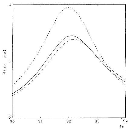
Figure 1: $Z$-line shape: Uncorrected (fine-dashed line); first order QED correction (dashed line); second order exponential corrections (solid line). From F. Berends[8].

Let me now turn to electroweak radiative corrections proper. The bulk of these corrections for the process $e^{+}e^{-}\to f\bar{f}$ arises from corrections to the gauge propagator. This is easy to understand since it is only here that different mass scales can enter at energy scales $\sqrt{s}\simeq M_{Z}$. The fermion loop in Fig. 2a contains both the scales $M_{Z}$ and $m_{f^{\prime}}$ and the corrections are of $O\left(\frac{\alpha}{\pi}\ln M_{Z}/m_{f^{\prime}}\right)$. In contrast, the box graph of Fig. 2b has only $M_{W}\simeq M_{Z}$ as the dominant scale and thus it contributes corrections only of $O\left(\frac{\alpha}{\pi}\right)$. Corrections due to the large top mass of $O\left(\frac{\alpha}{\pi}\frac{m_{t}^{2}}{M_{Z}^{2}}\right)$ also arise mostly through vacuum polarization corrections. The exception is the process $e^{+}e^{-}\to b\bar{b}$ which is sensitive to $m_{t}$ also as a result of the vertex graph shown in Fig. 3.

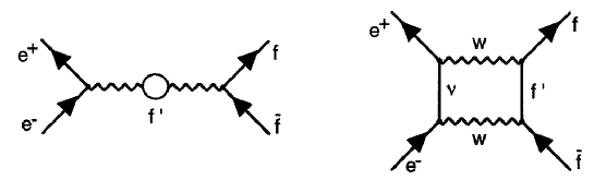
Figure 2: Corrections to the process $e^{+}e^{-}\to f\bar{f}$: (a) gauge propagator corrections;     (b) box graph corrections.

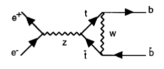
Figure 3: Vertex corrections to the process $e^{+}e^{-}\to b\bar{b}$ sensitive to the top mass.

Given the above, it is clear that to understand the principal features of electroweak radiative corrections it suffices for our purposes to look at the corrections to the gauge propagators. These corrections are known as oblique corrections[10]. A good starting point for our discussion are the modification to the lowest order photon exchange graph for the process $e^{+}e^{-}\to f\bar{f}$, shown in Fig. 4a. This graph leads to an amplitude

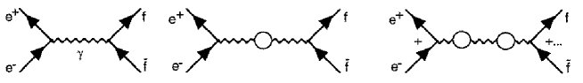
Figure 4: (a) Lowest order photon exchange process;     (b) Loop modifications to lowest order photon exchange process.

$$A^{o}_{\gamma}(e^{+}e^{-}\to f\bar{f})=q_{e}q_{f}\frac{e_{o}^{2}}{s}J_{\rm em}^{e}\cdot J^{f}_{\rm em}~{},$$ (32)

where $q_{e},q_{f}$ are the numerical values of the fermion electric charges in units of $e_{o}$. The collection of graphs in Fig. 4b produce a modification of the lowest order photon propagator $1/s$ and changes the bare charge $e_{o}$ into the physical charge $e$, defined here through its value in Thompson scattering at zero momentum transfer [$e=e(o)$]. One has

$$A_{\gamma}(e^{+}e^{-}\to f\bar{f})=q_{e}q_{f}[e^{2}\Delta_{\gamma}(s)]J^{e}_{\rm em}\cdot J^{f}_{\rm em}~{}.$$ (33)

In the above, the full propagator $\Delta_{\gamma}(s)$ contains the self-energy contributions $\Sigma_{\gamma}(s)\equiv s\Pi_{\gamma}(s)$:

$$\Delta^{-1}_{\gamma}(s)=s+\Sigma_{\gamma}(s)=s[1+\Pi_{\gamma}(s)]$$ (34)

The particular structure shown in Eq. (34) guarantees that indeed the photon exchange contribution has a pole at $s=0$, as required by gauge invariance. A comparison of Eq. (33) with Eq. (32) show that for the photon case, the effect of the radiative corrections is codified through the replacement:

$$\frac{e_{o}^{2}}{s}\to\frac{e^{2}}{s\left[1+\Pi_{\gamma}(s)\right]}\equiv\frac{e^{2}(s)}{s}~{},$$ (35)

with the “running coupling” $e^{2}(s)$ defined by

$$e^{2}(s)=\frac{e^{2}}{1+\Pi_{\gamma}(s)}~{}.$$ (36)

One can proceed in a similar fashion for the $Z$ exchange contribution. In this case, it is useful to write the inverse full propagator as

$$\Delta^{-1}_{Z}(s)=s-M^{2}_{Z}+\Sigma_{Z}(s)=s-M^{2}_{Z}+{\rm Re}~{}\Sigma_{Z}(s)+i~{}{\rm Im}~{}\Sigma_{Z}(s)$$ (37)

where $M_{Z}$ is the physical mass of the $Z$. Because $M_{Z}$ is the physical mass, to keep the pole location in the $Z$ propagator there, one needs to have

$${\rm Re}\Sigma_{Z}(s)=(s-M^{2}_{Z})\Pi_{Z}(s)~{}.$$ (38)

In contrast to the photon case, since the $Z$ has a physical decay channel into fermions $[Z\to f\bar{f}]$, one cannot ignore the imaginary part of the $Z$ self-energy. In fact, denoting schematically the coupling of the $Z$ to fermions by $g_{f}$, one has that

$${\rm Im}~{}\Sigma_{Z}(M^{2}_{Z})\sim\sum_{f}g_{f}^{2}~{}.$$ (39)

With the above definitions, one can rewrite the inverse $Z$ propagator as

$$\Delta^{-1}_{Z}(s)=[1+\Pi_{Z}(s)]\left\{s-M^{2}_{Z}+i\frac{{\rm Im}~{}\Sigma_{Z}(s)}{[1+\Pi_{Z}(s)]}\right\}~{}.$$ (40)

The last term in the curly bracket above serves to define an $s$-dependent $Z$ width:

$$M_{Z}\Gamma_{Z}(s)=\frac{{\rm Im}~{}\Sigma_{Z}(s)}{[1+\Pi_{Z}(s)]}~{}.$$ (41)

Note that if one defines, analogously to $e^{2}(s)$, a running coupling of the $Z$ to fermions via

$$g_{f}^{2}(s)=\frac{g^{2}_{f}}{[1+\Pi_{Z}(s)]}~{},$$ (42)

then one sees that the $Z$-width involves precisely the fermion couplings at this scale

$$\Gamma_{Z}=\Gamma_{Z}(M^{2}_{Z})\sim\sum_{f}g_{f}^{2}(M_{Z}^{2})~{},$$ (43)

as one would expect physically.

The radiatively corrected $Z$ contribution, analogous to Eq. (33), reads

$$A_{Z}(e^{+}e^{-}\to f\bar{f}) = g_{e}g_{f}[\Delta_{Z}(s)]J^{e}_{\rm NC}\cdot J^{f}_{\rm NC}$$ (44)

$$= \frac{g_{e}(s)g_{f}(s)}{s-M^{2}_{Z}+iM_{Z}\Gamma_{Z}(s)}J^{e}_{\rm NC}\cdot J^{f}_{\rm NC}$$

One sees that here also the radiative corrections just replace the bare couplings by the running couplings. In addition, the $Z$ propagator involves the physical $Z$ mass and an $s$-dependent width. Before the bremsstrahlung corrections, the amplitude in Eq. (44) near the energy corresponding to the $Z$ mass leads to a Breit-Wigner formula for the cross-section for $e^{+}e^{-}\to f\bar{f}$:

$$\sigma^{Z}_{\rm BW}(s)=\frac{12\pi\Gamma_{e}\Gamma_{f}}{M^{2}_{Z}}\left[\frac{s}{(s-M^{2}_{Z})^{2}+\Gamma^{2}_{Z}(s)M^{2}_{Z}}\right]~{}.$$ (45)

Since, approximately, $\Gamma_{Z}(s)$ is linear in $s$ near $\sqrt{s}\simeq M_{Z}$:

$$\Gamma_{Z}(s)=\frac{s}{M^{2}_{Z}}\Gamma_{Z}$$ (46)

it is easy to show that Eq. (45) has a maximum at

$$(\sqrt{s})_{\rm max}=M_{Z}-\frac{1}{4}\frac{\Gamma_{Z}^{2}}{M_{Z}}\simeq M_{Z}-17~{}{\rm MeV}~{}.$$ (47)

This small downward shift of the maximum is opposite to the much larger upward shift caused by initial state bremsstrahlung [cf Eq. (31)].

I anticipate here that the running couplings at $M_{Z}$ occurring in Eq. (44) can be written in terms of the Fermi constant measured in $\mu$-decay, the $Z$ mass and a $\rho$ parameter, which essentially measures the ratio of neutral current to charged current processes (and which will be defined more precisely shortly):

$$g_{e}(M^{2}_{Z})g_{f}(M^{2}_{Z})=\sqrt{2}G_{F}M_{Z}^{2}\rho~{}.$$ (48)

This formula is “sensible” since it just generalizes the lowest order result

$$g^{o}_{e}g_{f}^{o}=\frac{e_{o}^{2}}{4\sin^{2}\theta_{W}^{o}\cos\theta^{o}_{W}}=\sqrt{2}~{}G_{F}^{o}(M_{Z}^{o})^{2}\rho^{o}~{},$$ (49)

but remains to be proven. Using Eq. (48), one sees that one can incorporate the dominant (logarithmic) electroweak radiative corrections through an improved Born approximation[11] involving physically measured parameters—including appropriately defined $\sin^{2}\theta_{W}$ and $\rho$ parameters. One finds

$$A_{\rm Improved~{}Born}(e^{+}e^{-}\to f\bar{f})=q_{e}q_{f}\frac{e^{2}(s)}{s}J^{e}_{\rm em}\cdot J^{f}_{\rm em}+\frac{\sqrt{2}G_{F}M^{2}_{Z}\ J^{e}_{\rm NC}\cdot J^{f}_{\rm NC}}{s-M^{2}_{Z}+iM_{Z}\Gamma_{Z}(s)}~{},$$ (50)

where the electromagnetic and neutral currents contain the structures

$$(J^{f}_{\rm em})_{\mu}=\gamma_{\mu}~{};~{}~{}~{}(J^{f}_{\rm NC})_{\mu}=\gamma_{\mu}\left[t_{3f}(1-\gamma_{5})-2q_{f}\sin^{2}\theta_{W}\right]~{}.$$ (51)

In what follows, I elaborate further on the relation between the parameters $\rho$ and $\sin^{2}\theta_{W}$ appearing above and the bare parameters defined in Section 2.1.

2.3 Radiative Corrections: Leading Logs

It is important to understand the relation of the parameters in the improved Born approximation with the bare parameters which enter in the electroweak Lagrangian. The $SU(2)\times SU(1)$ theory has a number of these parameters: the $SU(2)$ and $U(1)$ couplings, $g_{o}$ and $g^{\prime}_{o}$; the Higgs VEV, $v_{o}$; the Yukawa couplings $\Gamma_{ij}^{f}$; and the Higgs self-coupling, which is associated with the bare Higgs mass. These parameters are modified by radiative corrections. In fact, when one calculates these corrections one finds that they are infinite. These infinities must be eliminated to obtain sensible physical results. Because the standard model is a renormalizable theory this can be done. It is achieved through a rescaling of the field appearing in the SM Lagrangian and by replacing the bare parameters in ${\cal{L}}_{\rm SM}$ by a set of renormalized (or physical) parameters:

$$\{g_{o};g_{o}^{\prime};v_{o},\Gamma^{f}_{ij},M^{o}_{H}\}\to\{g,g^{\prime},v,(\Gamma^{f}_{ij})_{\rm ren},M_{H}\}~{}.$$ (52)

These latter parameters are defined through their relation to specific measurements. Because of this, rather than the set of parameters in Eq. (52) which naturally enter in a Lagrangian description, it is more useful to choose a more physical set of parameters with which to characterize the theory.

The standard set of parameters which has been adopted in the literature to describe the electroweak theory replaces the set in Eq. (52) by

$$\{g,g^{\prime},v,(\Gamma^{f}_{ij})_{\rm ren},M_{H}\}\to\{e,G_{F},M_{Z},m_{f_{i}},V_{\rm CKM},M_{H}\}~{}.$$ (53)

Here $m_{f_{i}}$ are the physical fermion masses defined in terms of zeros in the inverse fermion propagators (analogous to those we discussed for the $Z$ boson) and $V_{\rm CKM}$ in the fermion mixing matrix. For the most part, when dealing with electroweak precision measurements at the $Z$ one can neglect all fermion masses, except for the top mass, and the effect of fermion mixing ($V_{\rm CKM}\to 1$). The electric charge in Eq. (53) is $e(o)$ defined through Thompson scattering, with $\alpha(o)=e^{2}(o)/4\pi\simeq 1/137$. $M_{Z}$ is the pole mass, as defined in Eq. (40), while $G_{F}$ is the Fermi constant as deduced from $\mu$-decay in the Fermi theory, with certain kinematical QED corrections included[12]. Having specified a standard set of parameters, then in the standard model all other measurable quantities (e.g. the mass of the $W$ boson) are predicted in terms of this standard set. Physical tests of the electroweak theory are provided by comparing the prediction for some measurable quantity with its experimentally measured value, e.g.

$$M_{W}\left|{}_{\rm theory}=M_{W}(e,G_{F},M_{Z},m_{t},M_{H})\leftrightarrow M_{W}\right|_{\rm exp}~{}.$$ (54)

It is worthwhile to illustrate the above discussion by considering in a bit more detail the connection of $G_{F}$—the Fermi constant—with $M_{W}$. As just indicated, $G_{F}$ is defined (essentially) as the effective coupling for $\mu$-decay in the Fermi theory:

$${\cal{L}}_{\rm eff}^{\rm Fermi}=\frac{G_{F}}{\sqrt{2}}(\mu^{-}\gamma^{\mu}(1-\gamma_{5})\nu_{\mu})(\bar{\nu}_{e}\gamma_{\mu}(1-\gamma_{5})e)~{}.$$ (55)

Using (55) the muon lifetime then provides a direct measure of $G_{F}$, through the standard formula $\tau^{-1}_{\mu}=G_{F}^{2}m^{5}_{\mu}/192\pi^{3}$. This formula is modified by pure QED corrections—which are included in the proper definition of $G_{F}$—as these photonic radiative corrections are finite (see below).

If one thinks of Eq. (55) as an effective approximation of the standard model Lagrangian for values of $q^{2}\ll M^{2}_{W}$, then one would naively expect the coefficient of the four-fermion operator, $G_{F}$, to be scale-dependent. Photon exchange corrections should contribute to the running of $G_{F}$ from the scale $\mu^{\prime 2}$ to the scale $\mu^{2}$:

$$G_{F}(\mu^{2})=G_{F}(\mu^{\prime 2})\left[\frac{\alpha(\mu^{\prime 2})}{\alpha(\mu^{2})}\right]^{d_{\gamma}}~{},$$ (56)

with $d_{\gamma}$ being the anomalous dimension of the 4-Fermi operator in Eq. (55). However, because photon corrections to the effective Lagrangian (55) give only finite corrections, the anomalous dimension $d_{\gamma}$ vanishes. Thus $G_{F}(\mu^{2})$ is independent of the scale $\mu^{2}$: $G_{F}(\mu^{2})\equiv G_{F}$. This fact can be easily demonstrated by a Fierz rotation of Eq. (55), which yields

$${\cal{L}}_{\rm eff}^{\rm Fermi}=\frac{G_{F}}{\sqrt{2}}(\bar{\mu}\gamma^{\mu}(1-\gamma_{5})e)(\bar{\nu}_{e}\gamma_{\mu}(1-\gamma_{5})\nu_{\mu})~{}.$$ (57)

The second current above, clearly gets no photonic corrections. So the anomalous dimension $d_{\gamma}$ is that associated with the $\mu-e$ current. However, this current incurs no logarithmic corrections since it is conserved in the limit of neglecting the $\mu$ and $e$ masses. Thus, efffectively, $d_{\gamma}=0$.

With these considerations, it is easy to convince oneself that to logarithmic accuracy the effect of radiative corrections is to transcribe directly the bare relationship between $G_{F}^{o}$ and $M_{W}^{o}$ into a relationship between physical quantities. The bare equation

$$\frac{G_{F}^{o}}{\sqrt{2}}=\frac{e_{o}^{2}}{8\sin^{2}\theta_{W}(M_{W}^{o})^{2}}=\frac{e_{o}^{2}}{8\left[1-\left(\frac{M_{W}^{o}}{M_{Z}^{o}}\right)^{2}\right](M_{W}^{o})^{2}}$$ (58)

becomes, in leading log approximation, a relation between physically measured quantities. Provided all quantities are measured at the same scale[13], this equation will have precisely the same form as the bare equation. Thus Eq. (58) is replaced by

$$\frac{G_{F}}{\sqrt{2}}=\frac{e^{2}(M_{Z}^{2})}{8\left[1-\left(\frac{M_{W}}{M_{Z}}\right)^{2}\right]M^{2}_{W}}~{}.$$ (59)

The RHS of Eq. (59) contains only quantities measured at the scale of the weak boson masses $M_{W}\cong M_{Z}$ and, because $G_{F}$ is scale independent, indeed that is also the scale of the LHS. Thus, a fortiori, Eq. (59) is the correct result! One sees that in relating $M_{W}$ to the standard set of Eq. (53), all radiative corrections—in leading log approximation—are contained in the running of the electromagnetic charge from $e^{2}(o)$ to $e^{2}(M^{2}_{Z})$. Defining, as usual, $\alpha(M^{2}_{Z})=\frac{e^{2}(M_{Z}^{2})}{4\pi}$ one has the standard model interrelation

$$G_{F}=\frac{\pi\alpha(M^{2}_{Z})}{\sqrt{2}~{}M^{2}_{W}\left[1-M^{2}_{W}/M^{2}_{Z}\right]}~{},$$ (60)

which predicts $M_{W}$ in terms of the standard set of parameters.

In a similar way, also the Weinberg angle can be considered as a derived quantity in terms of the standard set of parameters. Recall for these purposes the different ways in which the Weinberg angle was defined at the Lagrangian level in terms of bare parameters:

(i) Through the unification condition

$$e_{o}=g_{o}\sin\theta_{W}^{o}=g^{\prime}_{o}\cos\theta_{W}^{o}~{}.$$ (61)

(ii) Via the $M_{W}^{o}-M_{Z}^{o}$ relation (doublet Higgs breaking)

$$\sin^{2}\theta_{W}^{o}=1-\left(\frac{M_{W}^{o}}{M_{Z}^{o}}\right)^{2}~{}.$$ (62)

(iii) By comparison to the Fermi theory

$$\frac{G_{F}^{o}}{\sqrt{2}}=\frac{e_{o}^{2}}{8\sin^{2}\theta_{W}^{2}(M_{W}^{o})^{2}}~{}.$$ (63)

(iv) Through the definition of the neutral current, $J^{\mu}_{\rm NC}$,

$$J^{\mu}_{\rm NC}=2(J^{\mu}_{3}-\sin^{2}\theta^{o}_{W}J^{\mu}_{\rm em})~{}$$ (64)

One can define different renormalized $\sin^{2}\theta_{W}$ by appropriately generalizing the above definitions. In general, however, each of these renormalized $\sin^{2}\theta_{W}$ will be given by a slightly different function of the standard set of parameters.

I illustrate the preceding discussion by means of two examples. In the first of these, the Weinberg angle is given its most physical definition by relating it directly to the $W$ and $Z$ masses. This is the definition first adopted by Sirlin[14] and one has

$$[\sin^{2}\theta_{W}]_{s}=1-M^{2}_{W}/M^{2}_{Z}~{}.$$ (65)

From our discussion above of the relation of $G_{F}$ to $M_{W}$, it is easy to see that $[\sin^{2}\theta_{W}]_{s}$ when expressed in terms of the standard set of electroweak parameters is given (to logarithmic accuracy) by:

$$[\sin^{2}\theta_{W}]_{s}~{}[\cos^{2}\theta_{W}]_{s}=\frac{\pi\alpha(M^{2}_{Z})}{\sqrt{2}~{}G_{F}M^{2}_{Z}}~{}.$$ (66)

The second example of a renormalized $\sin^{2}\theta_{W}$ which is useful to consider is the effective $\sin^{2}\theta_{W}$ which appears in the expression for the neutral current in the improved Born approximation at the $Z$ resonance:

$$J^{\mu}_{\rm NC}=2(J^{\mu}_{3}-\sin^{2}\theta_{\rm eff}J^{\mu}_{\rm em})~{}.$$ (67)

It is this parameter $\sin^{2}\theta_{\rm eff}$ which is measured at LEP and the SLC. More precisely, $\sin^{2}\theta_{\rm eff}$ is to be thought of as the running parameter which multiplies $J^{\mu}_{\rm em}$ in $J^{\mu}_{\rm NC}$ at the scale $\mu^{2}=M^{2}_{Z}$. That is

$$\sin^{2}\theta_{\rm eff}=\sin^{2}\theta_{W}(M^{2}_{Z})~{}.$$ (68)

In the Glashow-Salam-Weinberg model, the running parameter $\sin^{2}\theta_{W}(\mu^{2})$ is related to $[\sin^{2}\theta_{W}]_{s}$, with the constant of proportionality being a finite calculable quantity:

$$\sin^{2}\theta_{W}(\mu^{2})=\kappa(\mu^{2})[\sin^{2}\theta_{W}]_{s}~{}.$$ (69)

A calculation of $\kappa(\mu^{2})$[15], again to logarithmic accuracy, shows that this parameter depends on the scale $\mu^{2}$ as:

$$\kappa(\mu^{2})=1+\frac{\alpha}{8\pi[\sin^{2}\theta_{W}]_{s}}\left\{\sum_{f}(t_{3f}q_{f}-2q_{f}^{2}[\sin^{2}\theta_{W}]_{s})-1\right\}\ln M^{2}_{Z}/\mu^{2}~{}.$$ (70)

Obviously, in view of Eqs. (68-70), in leading log approximation there is no difference between $\sin^{2}\theta_{\rm eff}$ and $[\sin^{2}\theta_{W}]_{s}$. However, these quantities differ by the way they depend on $m^{2}_{t}$, as will be seen in the next section.

The above discussion serves to justify Eq. (48), which in the improved Born approximation replaced the product of the effective couplings of the electron and the outgoing fermion to the $Z$ by the Fermi constant, times the $Z$ mass squared, times $\rho$. The coefficient of the effective $Z$ propagator in the improved Born approximation involves

$${\rm Coeff}=\frac{e^{2}}{4[\sin^{2}\theta_{W}][\cos^{2}\theta_{W}]}\frac{1}{[1+\Pi_{Z}(M_{Z}^{2})]}~{}.$$ (71)

Using the relation (66) and the definition (36), the above can be rewritten as

$${\rm Coeff}=\sqrt{2}~{}G_{F}M^{2}_{Z}\frac{[1+\Pi_{\gamma}(M^{2}_{Z})]}{[1+\Pi_{Z}(M^{2}_{Z})]}~{}.$$ (72)

Because in the leading log approximation the only running is that of $\alpha$, effectively the ratio of the vacuum polarization functions in Eq. (72) is unity. Furthermore, because $M_{W}\simeq M_{Z}$, the ratio of NC/CC contributions also does not pick up any logarithmic factor. Hence if one has doublet Higgs breaking, so that $\rho^{o}=1$, then in leading log approximation $\rho=1$. Whence, to this accuracy, (72) can be written as

$${\rm Coeff}=\sqrt{2}~{}G_{F}M^{2}_{Z}\rho~{},$$ (73)

which proves our contention. However, as we will see, the $\rho$ parameter does depend on $m^{2}_{t}$ and it deviates from unity as a result of these effects.

2.4 Radiative Corrections: $m_{t}$ Effects

It turns out that the sensitivity to the top mass of physical observables can all be related to the $m_{t}$ dependence of the $\rho$ parameter, detailing the ratio of NC to CC processes. If one examines the radiative corrections to the gauge propagators entering in NC and CC processes, it is easy to see that in the Fermi limit, the $\rho$ parameter differs from unity only to the extent that the $Z$ and $W$ self-energies are different from each other

$$\rho=1+\left[\frac{\Sigma_{Z}(o)}{M^{2}_{Z}}-\frac{\Sigma_{W}(o)}{M^{2}_{W}}\right]=1-\left[\Pi_{Z}(o)-\Pi_{W}(o)\right]~{}.$$ (74)

To compute the vacuum polarization difference in Eq. (74) it suffices to retain the $t$ and $b$ loops in $\Pi_{Z}(o)$ and the $t-b$ loop for $\Pi_{W}(o)$. Furthermore, since electromagnetic interactions do not give rise to contributions proportional to the fermion mass in the loop, it suffices to retain only the $J^{\mu}_{3}$ piece in $J^{\mu}_{\rm NC}$ for this calculation. A simple computation then shows that

$$\Pi_{Z}(o)-\Pi_{W}(o) = -\frac{3i\alpha}{8\pi^{3}M^{2}_{W}\sin^{2}\theta_{W}}\cdot\int d^{4}p$$ (75)

$$\times \left[\frac{1}{(p^{2}+m^{2}_{t})^{2}}+\frac{1}{(p^{2}+m_{b}^{2})^{2}}-\frac{2}{(p^{2}+m_{b}^{2})(p^{2}+m_{t}^{2})}\right]$$

$$= -\frac{3\alpha}{16\pi\sin^{2}\theta_{W}}\left(\frac{m_{t}}{M_{W}}\right)^{2}~{},$$

where we have dropped terms of $O(m_{b}^{2})$ relative to those of $O(m_{t}^{2})$. It follows therefore that

$$\rho=1+\frac{3G_{F}}{8\sqrt{2}\pi^{2}}m_{t}^{2}~{},$$ (76)

a formula first obtained by Veltman[16], which shows that $\rho$ is quadratically sensitive to the top mass.

To deduce the $m_{t}$ dependence of other parameters in the theory one can argue as follows. The renormalized parameters follow from the bare parameters by a shift in these parameters. Thus to trace the $m_{t}$ dependence it suffices to track the $m_{t}$ sensivity of these shifts. As an example, consider the Fermi formula, Eq. (16). The zero order formula, $G_{F}^{o}=\frac{\pi\alpha^{o}}{\sqrt{2}~{}\sin^{2}\theta_{W}^{o}(M_{W}^{o})^{2}}$, after shifts in the bare parameters leads to the corrected formula [cf. Eq. (66)]

$$G_{F}=\frac{\pi\alpha(M^{2}_{Z})}{\sqrt{2}[\sin^{2}\theta_{W}]_{s}[\cos^{2}\theta_{W}]_{s}M^{2}_{Z}}f(m_{t}^{2})~{}.$$ (77)

Here the function $f(m_{t}^{2})$ differs from unity only through the $m_{t}$ dependence arising from the shifts in $\sin^{2}\theta_{W}^{o}$. This is because there is no $m_{t}$ dependence in the shift of the electric charge squared, $\delta\alpha^{o}$, and the $m_{t}$ dependence of $\delta G_{F}^{o}$ and $\delta(1/(M_{W}^{o})^{2})$ cancel each other. Now for the bare quantities one has $\sin^{2}\theta_{W}^{o}=1-(M_{W}^{o})^{2}/(M_{Z}^{o})^{2}$, so that

$$\delta\sin^{2}\theta_{W}^{o}=[\cos^{2}\theta_{W}]_{s}\left\{\frac{(\delta M_{Z}^{o})^{2}}{(M_{Z}^{o})^{2}}-\frac{(\delta M_{W}^{o})^{2}}{(M_{W}^{o})^{2}}\right\}~{}.$$ (78)

In the limit $m_{t}\gg M_{W},M_{Z}$, the mass shifts in Eq. (78) can be related to the $\rho$ parameter since

$$(\delta M_{Z}^{o})^{2}=-\Sigma^{o}_{Z}(M_{Z}^{2})\simeq-\Sigma_{Z}^{o}(o);~{}~{}(\delta M_{W}^{o})^{2}=-\Sigma_{W}^{o}(M^{2}_{W})\simeq-\Sigma_{W}^{o}(o)~{},$$ (79)

so that

$$\delta\sin^{2}\theta_{W}^{o}\simeq[\cos^{2}\theta_{W}]_{s}[\rho-1]~{}.$$ (80)

It follows, therefore, that

$$f(m_{t}^{2})=\frac{1}{1+\frac{\delta\sin^{2}\theta_{W}^{o}}{[\sin^{2}\theta_{W}]_{s}}}=\frac{1}{1+\frac{\cos^{2}\theta_{W}}{\sin^{2}\theta_{W}}\Delta\rho}~{},$$ (81)

where, using Eq. (76),

$$\Delta\rho=\frac{3G_{F}}{8\sqrt{2}\pi^{2}}m_{t}^{2}~{}.$$ (82)

Thus, including not only leading log contributions but also $m_{t}^{2}$ effects, one can express $[\sin^{2}\theta_{W}]_{s}$ (or equivalently $M_{W}^{2}$) in terms of the standard set of parameters via the formula

$$[\sin^{2}\theta_{W}]_{s}[\cos^{2}\theta_{W}]_{s}=\frac{\pi\alpha(m^{2}_{Z})}{\sqrt{2}G_{F}M^{2}_{Z}}\frac{1}{1+\frac{[\cos^{2}\theta_{W}]_{s}\Delta\rho}{[\sin^{2}\theta_{W}]_{s}}}~{}.$$ (83)

Similar considerations lead to the following expression for the radiatively corrected $\sin^{2}\theta_{\rm eff}$ (leading log plus $m_{t}^{2}$ corrections):

$$\sin^{2}\theta_{\rm eff}=[\sin^{2}\theta_{W}]_{s}+\Delta\rho[\cos^{2}\theta_{W}]_{s}$$ (84)

which leads to the result

$$\sin^{2}\theta_{\rm eff}\cos^{2}\theta_{\rm eff}=\frac{\pi\alpha(m^{2}_{Z})}{\sqrt{2}G_{F}M^{2}_{Z}}\frac{1}{1+\Delta\rho}~{}.$$ (85)

Since $\sin^{2}\theta_{W}\simeq 0.25$, it is clear from Eqs. (83) and (85) that $[\sin^{2}\theta_{W}]_{s}$ depends more strongly on the value of the top mass than $\sin^{2}\theta_{\rm eff}$.

The quantity

$$s_{o}^{2}c_{o}^{2}=\frac{\pi\alpha(m^{2}_{Z})}{\sqrt{2}G_{F}M^{2}_{Z}}$$ (86)

entering in both Eqs. (83) and (85) is extremely well known experimentally, with its principal error arising from the error which enters in running $\alpha$ to the $Z$ mass: $\alpha(M^{2}_{Z})=[129\pm 0.1]^{-1}$[17]. One finds

$$s_{o}^{2}c_{o}^{2}=0.17755\pm 0.00014$$ (87)

leading to $s_{o}^{2}=0.2309\pm 0.0003$. Unfortunately, it appears difficult to improve the error on $\alpha(M_{Z})$, since it arises principally from errors in the low energy data on $e^{+}e^{-}\to{\it hadrons}$ needed to estimate the contributions of the hadronic vacuum polarization to the running of $\alpha$[17]. As we shall see $\pm 0.0003$ is the size of the experimental error on the value of $\sin^{2}\theta_{\rm eff}$ determined by precision electroweak data, so already this error is comparable to the “standard error” arising due to our imperfect knowledge of $\alpha(M_{Z}^{2})$!

I note that Eqs. (83) and (85) only contain the dominant contributions of the electroweak radiative corrections. For detailed comparisons with precision data one must really use the full formulas, which include both terms of $O\left(\frac{\alpha}{\pi}\right)$ and corrections that depend on the Higgs mass $M_{H}$. These latter corrections are infinite in the limit as $M_{H}\to\infty$, since the standard model becomes a non-renormalizable theory in this limit. It was shown by Veltman[18] that the sensitivity of the electroweak corrections to $M_{H}$ is only logarithmic in lowest order in $\alpha$, becoming quadratic at $O(\alpha^{2})$[19]. Detailed calculations give, for example, for large $M_{H}$ the formulas[20]

$$\rho=1+\frac{3G_{F}}{8\sqrt{2}\pi^{2}}m_{t}^{2}-\frac{3G_{F}M_{Z}^{2}}{4\sqrt{2}\pi^{2}}s_{o}^{2}\ln M_{H}/M_{Z}+\ldots\equiv 1+\Delta\rho$$ (88)

$$\sin^{2}\theta_{\rm eff}=s_{o}-\frac{c_{o}^{2}}{c_{o}^{2}-s_{o}^{2}}\left\{\Delta\rho-\frac{G_{F}M_{Z}^{2}}{12\sqrt{2}\pi^{2}}\ln M_{H}/M_{Z}+\ldots\right\}~{}.$$ (89)

One sees from the above that for large $M_{H}$ the effect of having a large top mass is partly cancelled in $\Delta\rho$. Furthermore, for large $M_{H}$ one can actually change the sign of the correction to $\sin^{2}\theta_{\rm eff}$, so that $\sin^{2}\theta_{\rm eff}>s_{o}^{2}$—as seen experimentally.

2.5 Comparison with Experiment

A convenient way to compare precision data from LEP and SLC (plus low energy neutrino scattering data and the value of $M_{W}$ measured at the $p\bar{p}$ colliders) with theoretical expectations is to refer everything back to $\sin^{2}\theta_{\rm eff}$, keeping $m_{t}$ and $M_{H}$ as free parameters which are then fit to the data. We do not know anything about $M_{H}$, except for the LEP bound that $M_{H}\geq 66~{}{\rm GeV}$[21]. On the other hand, new and precise information is being gathered on $m_{t}$ at the Fermilab Tevatron. At the time of TASI ’96, the value I quoted for $m_{t}$ was that given in the 1996 Winter conferences. This value is now superseded, because more data has been analyzed by the CDF and DO Collaborations. The value of $m_{t}$ obtained by combining the latest CDF and DO results is[22]

$$m_{t}=(175\pm 6)~{}{\rm GeV}~{},$$ (90)

which is already amazingly accurate and provide strong constraints on the theory.

Using the improved Born approximation, Eq. (50), it is straightforward to derive formulas for various measurable quantities. I summarize some of these results below:

Leptonic Width. The width for the process $Z^{o}\to\ell\bar{\ell}~{}(\ell=e,\mu,\tau)$, in the limit where one neglects the lepton mass, is given by

$$\Gamma_{\ell}=\frac{G_{F}M_{Z}^{3}}{6\pi\sqrt{2}}[g^{2}_{V\ell}+g^{2}_{A\ell}]\left(1+\frac{3\alpha}{4\pi}\right)$$ (91)

where the last factor is a QED correction accounting for radiative leptonic decays. In the above, the vector and axial couplings in the standard model are universal and are given by

$$g^{2}_{V\ell}=\frac{1}{4}\rho[1-4\sin^{2}\theta_{\rm eff}]^{2}~{};~{}~{}~{}g^{2}_{A\ell}=\frac{1}{4}\rho~{}.$$ (92)

Forward-Backward Asymmetry. The number of fermions $f$ produced in the direction of the incoming electron $(\theta\leq\pi/2)$ compared to those produced in the backward direction has a simple form on resonance

$$A^{f}_{FB}=\frac{\sigma^{f}(\theta\leq\pi/2)-\sigma^{f}(\theta\geq\pi/2)}{\sigma^{f}(\theta\leq\pi/2)+\sigma^{f}(\theta\geq\pi/2)}|_{\rm Res}=\frac{3}{4}{\cal{A}}^{e}{\cal{A}}^{f}~{},$$ (93)

where

$${\cal{A}}^{f}=\frac{2g_{Vf}g_{Af}}{g^{2}_{Vf}+g^{2}_{Af}}~{},$$ (94)

with the vector and axial couplings of the fermion $f$ being defined analogously to Eq. (92). One sees that already from $\Gamma_{\ell}$ and $A^{\ell}_{FB}$ it is possible to determine $\rho$ and $\sin^{2}\theta_{\rm eff}$. However, there are further (redundant) measurements one can make.

$\tau$-Polarization Asymmetry. This asymmetry measures the difference between the cross section for producing right-polarized taus and left-polarized taus at resonance

$$P_{\tau}=\frac{\sigma_{\tau_{\rm R}}-\sigma_{\tau_{\rm L}}}{\sigma_{\tau_{\rm R}}+\sigma_{\tau_{\rm L}}}|_{\rm Res}~{}.$$ (95)

This asymmetry can be determined by analyzing the angular distribution of the $\tau$ decay-products. The actual value of $P_{\tau}$ depends in detail on the production angle $\theta$ of the $\tau^{-}$, relative to the incoming electron. After a simple calculation one deduces

$$P_{\tau}(\cos\theta)=-\frac{{\cal{A}}^{\tau}(1+\cos^{2}\theta)+2{\cal{A}}^{e}\cos\theta}{1+\cos^{2}\theta+2{\cal{A}}^{\tau}{\cal{A}}^{e}\cos\theta}~{}.$$ (96)

By analyzing the dependence of $P_{\tau}$ on $\cos\theta$ in detail, one can extract from the data independently ${\cal{A}}^{\tau}$ and ${\cal{A}}^{e}$—which, of course, should coincide in the standard model.

Left-Right Asymmetry. This is a quantity that requires an initially polarized $e^{-}$ beam and can be measured only at the SLC where beams with a high longitudinal polarization $(\langle P_{e}\rangle\simeq 80\%)$ can be produced. The Left-Right asymmetry measures the difference in cross-section between beams which are either left- or right-polarized. On resonance, one has

$$A_{\rm LR}=\frac{\sigma(e^{-}_{\rm L})-\sigma(e^{-}_{\rm R})}{\sigma(e^{-}_{\rm L})+\sigma(e^{-}_{\rm R})}=\langle P_{e}\rangle{\cal{A}}^{e}$$ (97)

Note that $A_{\rm LR}$, as well as the $\tau$-polarization asymmetry, depend on a quantity ${\cal{A}}^{\ell}$ which is approximately linear in $1-4\sin^{2}\theta_{\rm eff}~{}[{\cal{A}}^{\ell}\simeq 2(1-4\sin^{2}\theta_{\rm eff})]$, while the Forward-Backward asymmetry $A^{\ell}_{\rm FB}$ is quadratic in $1-4\sin^{2}\theta_{\rm eff}$. Thus, since $\sin^{2}\theta_{\rm eff}\simeq 0.25$, the error on this quantity is under much better control in $A_{\rm LR}$ than in $A^{\ell}_{FB}$.

I summarize below the results of LEP and SLC using the 1995 data set. These results have been updated for the 1996 Summer conferences, with no major changes (except in one area to be discussed further below). Because of this, and because all the 1995 data is collected together in a joint publication[23], I decided to use this slightly older data set for comparison of experiment with theory. The data is totally consistent with lepton universality, so I will quote only the combined result for all three leptons species obtained upon averaging the four LEP experiments. The leptonic width and the leptonic Forward-Backward asymmetry at LEP are found to be[23]

$$\Gamma_{\ell} = (83.93\pm 0.141)~{}{\rm MeV}$$ (98)

$$A^{\ell}_{\rm FB} = 0.0172\pm 0.0012~{}.$$ (99)

The result from the $\tau$-Polarization asymmetry from LEP, when one combines the independent (but consistent) values obtained for ${\cal{A}}^{e}$ and ${\cal{A}}^{\tau}$ gives

$${\cal{A}}^{\ell}_{\rm LEP}=0.1406\pm 0.0057~{}.$$ (100)

From the Left-Right asymmetry measured at the SLC one obtains a, somewhat higher, value for this quantity—although consistent within errors:

$${\cal{A}}^{\ell}_{\rm SLC}=0.1551\pm 0.0040~{}.$$ (101)

The value of Eq. (99) for $A^{\ell}_{\rm FB}$, using lepton universality, allows one to infer another independent determination of ${\cal{A}}^{\ell}$ and one finds

$${\cal{A}}^{\ell}_{\rm FB}=0.1514\pm 0.0053~{}.$$ (102)

The average of the three measurements (100)-(102) gives, finally,

$$\langle{\cal{A}}^{\ell}\rangle=0.1506\pm 0.0028~{}.$$ (103)

From the results for $\Gamma_{\ell}$ and $\langle{\cal{A}}^{\ell}\rangle$ one can infer values for $g_{V\ell}$ and $g_{A\ell}$ or equivalently, for $\rho$ and $\sin^{2}\theta_{\rm eff}$. Assuming the signs of the standard model, one finds

$$g_{V\ell}=-0.03799\pm 0.00071~{};~{}~{}~{}g_{A\ell}=-0.50111\pm 0.00041$$ (104)

and the (leptonic) results

$$\rho = 1.0044\pm 0.0012$$ (105)

$$\sin^{2}\theta_{\rm eff}|_{\rm leptons} = 0.23106\pm 0.00035~{}.$$ (106)

As can be seen from Fig. 5, these leptonic results are in very good agreement with the Glashow-Salam-Weinberg theory for $60~{}{\rm GeV}<M_{H}<1000~{}{\rm GeV}$ and $m_{t}=(180\pm 12)~{}{\rm GeV}$.

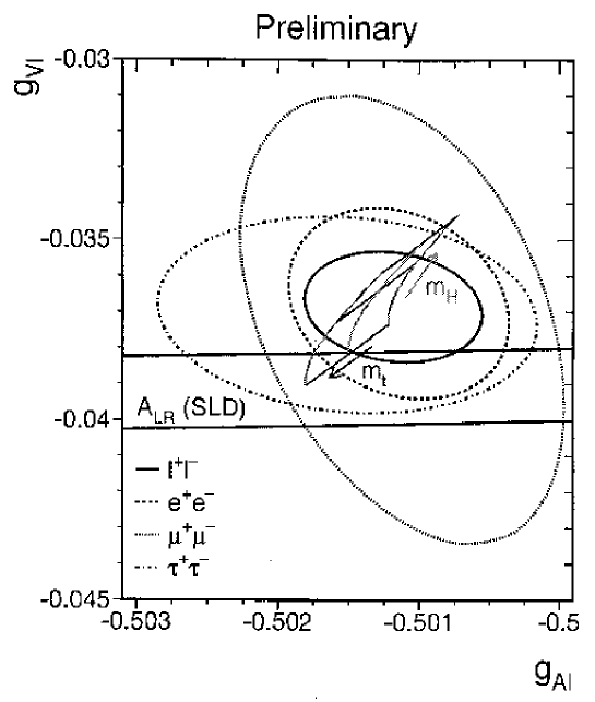
Figure 5: $1\sigma$ contours in the $g_{V\ell}-g_{A\ell}$ plane. The solid contour assumes lepton universality. Also shown is the $1\sigma$ band from the $A_{\rm LR}$ measurement. The grid corresponds to the standard model prediction for $m_{t}=180\pm 12~{}{\rm GeV}$ and the full Higgs mass range. The arrows point in the direction of increasing value of $m_{t}$ and $M_{H}$. From [23].

Further information on $\sin^{2}\theta_{\rm eff}$ comes from the LEP measurements of the Forward-Backward asymmetry of heavy quarks ($b$ and $c$). From these measurements[23] one can infer values for ${\cal{A}}^{b}=0.871\pm 0.029$ and ${\cal{A}}^{c}=0.635\pm 0.046$, which imply the (quark) result for the Weinberg angle:

$$\sin^{2}\theta_{\rm eff}|_{\rm quarks}=0.23205\pm 0.00051~{}.$$ (107)

The combined result of all measurements, both leptonic and quark, gives finally a value for $\sin^{2}\theta_{\rm eff}$ which is accurate to 1 part in $10^{3}$:

$$\sin^{2}\theta_{\rm eff}=0.23143\pm 0.00028~{}.$$ (108)

From this result, in the standard model, one can infer a value for the top mass, as a function of the Higgs mass. The value so obtained in[23] is

$$m_{t}=180^{+8+17}_{-9-19}{\rm GeV}$$ (109)

The second error above comes from allowing the Higgs mass to vary from $M_{H}=60~{}{\rm GeV}$ to $M_{H}=1000~{}{\rm GeV}$. The central value in Eq. (109) is that corresponding to assuming $M_{H}=300~{}{\rm GeV}$, with lower Higgs masses serving to decrease this value. Obviously, the indirect determination of $m_{t}$ through the standard model radiative corrections is in excellent agreement with the direct measurement of the top mass at the Tevatron, Eq. (90).

Individual measurement of various other electroweak quantities are also in excellent agreement with the standard model[23] except perhaps (at least for the 1995 data!) for the ratios $R_{b}$ and $R_{c}$, which measure the ratio of $Z\to b\bar{b},~{}c\bar{c}$ compared to the total hadronic rate. The values that one deduces for $M_{W}$ and $[sin^{2}\theta_{W}]_{s}$ from the standard model fit, using $m_{t}=180~{}{\rm GeV}$, are also in very good agreement with direct measurements. For $M_{W}$ one predicts[23]

$$M_{W}|_{\rm SM}=\left(80.359\pm 0.051\pm^{0.023}_{0.024}\right)~{}{\rm GeV}~{},$$ (110)

to be compared to the average value measured at the collider[24]

$$M_{W}=(80.356\pm 0.125)~{}{\rm GeV}~{}.$$ (111)

Similarly, for $[\sin^{2}\theta_{W}]_{s}$ the prediction is[23]

$$[\sin^{2}\theta_{W}]_{s}|_{\rm SM}=0.2234\pm 0.0009^{+0.0005}_{-0.0012}~{},$$ (112)

while the value one infers from deep inelastic neutrino scattering is

$$[\sin^{2}\theta_{W}]_{s}=0.2257\pm 0.0047~{}.$$ (113)

2.6 The $R_{b}-R_{c}$ Problem and its Resolution

The 1995 precision electroweak data has one blemish. The values of the ratios

$$R_{b}=\frac{\Gamma(Z\to b\bar{b})}{\Gamma(Z\to{\rm hadrons})}~{};~{}~{}~{}R_{c}\equiv\frac{\Gamma(Z\to c\bar{c})}{\Gamma(Z\to{\rm hadrons})}$$ (114)

appear to be in significant contradiction with the expectations of the standard model. The measured numbers are[23]

$$R_{b}=0.2219\pm 0.0017~{};~{}~{}~{}R_{c}=0.1543\pm 0.0074~{},$$ (115)

while one expects in the standard model (for $m_{t}=180~{}{\rm GeV}$ and $M_{H}\equiv 300~{}{\rm GeV}$)

$$R_{b}|_{\rm SM}=0.2156~{};~{}~{}~{}R_{c}|_{\rm SM}=0.1724~{}.$$ (116)

These are difficult measurements and, furthermore, the measurements are correlated. Thus, the $3.5\sigma$ discrepancy in $R_{b}$ and the $2.5\sigma$ discrepancy in $R_{c}$ are perhaps not so serious. Indeed, if instead of using the measured value for $R_{c}$ in trying to subtract the background in the $R_{b}$ measurement, one uses the standard model value for $R_{c}$ then the experimental value of $R_{b}$ changes to

$$R_{b}=0.2205\pm 0.0016~{}~{}~{}~{}~{}~{}~{}[R_{c}=R_{c}|_{\rm SM}]~{}.$$ (117)

At TASI, I indicated that the attitude towards these results is physicist dependent, with some believing that the source of the possible discrepancy is due to experimental error in identifying heavy flavor events, while others take this discrepancy seriously and try to find some new physics phenomena to account for the measured values of $R_{b}$ and $R_{c}$. As a result of new data which was presented at the Warsaw International Conference on High Energy Physics in July and at the DPF Meeting in Minneapolis in August, it now appears that the 1995 results for $R_{b}$ and $R_{c}$ are not to be trusted. For instance, the ALEPH Collaboration [25] at LEP and the SLD Collaboration[26] at the SLC, as a result of new analysis, now find (for $R_{c}=R_{c}|_{\rm SM}$)

$$R_{b}|_{\rm ALEPH} = 0.2158\pm 0.0009\pm 0.0011$$ (118)

$$R_{b}|_{\rm SLD} = 0.2149\pm 0.0033\pm 0.0021~{}.$$ (119)

These numbers are in excellent agreement with the standard model expectations. Similarly, ALEPH[27] gives a value for $R_{c}$ which, given its large error, seems much more compatible with the value expected in the standard model

$$R_{c}|_{\rm ALEPH}=0.1683\pm 0.0091~{}.$$ (120)

It is interesting to understand the reason for the changes between the 95 and 96 results. Basically these can be ascribed to a better understanding of the efficiencies for detecting heavy quarks and the degree of correlation present when one requires that 2 heavy flavor decays are both detected in one event. Although one can measure independently the efficiencies for measuring a $b$-decay or $c$-decay, the different techniques used all have different backgrounds that must be considered. For example, using events where one just tags one $b$-decay, the quantity $R_{b}$ can be extracted from the number of tagged events once one knows the efficiencies $\epsilon_{b}$ for detecting $b$-decay events and $\epsilon_{c}$ for excluding $c$-decay events:

$$N_{\rm tag}=2N_{\rm hadronic}\{\epsilon_{b}R_{b}+\epsilon_{c}R_{c}\}~{}.$$ (121)

Similarly, using events where 2 heavy flavor decays are tagged, to extract $R_{b}$ one needs to know in addition the tagging efficiency correlation $C$ for tagging simultaneously two such events:

$$N_{\rm 2~{}tag}=N_{\rm hadronic}C\{\epsilon_{b}^{2}R_{b}+\epsilon^{2}_{c}R_{c}\}~{}.$$ (122)

If $\epsilon_{c}$ is small (as it is) and the tagging efficiency correlation $C=1$, then one can determine $R_{b}$ without having to know precisely the $b$ tagging efficiency $\epsilon_{b}$. In this case,

$$R_{b}=\frac{(N_{\rm tag})^{2}}{4N_{\rm hadronic}N_{\rm 2~{}tag}}~{};~{}~{}~{}\epsilon_{b}=\frac{2N_{\rm 2~{}tag}}{N_{\rm tag}}~{}.$$ (123)

The new analysis of ALEPH uses the data itself to determine the correlation efficiency $C$. This is important, even though $C$ is very near unity, since the purported accuracy for mesuring $R_{b}$ is at the percent level. Hence the results of the new analysis are more reliable than those reported in 95.

Even though the $R_{b}-R_{c}$ crisis is now gone, it might be worthwhile recalling here some of the theoretical disquisitions which were advanced to “resolve” this discrepancy, since they illustrate the kind of tight constraints that one has as a result of the success, otherwise, of the standard model in describing data. If $R_{b}$ is anomalous but $R_{c}$ is OK, then from the precision value of the hadronic width measured at LEP

$$\Gamma_{\rm hadronic}=(1744.8\pm 3.0)~{}{\rm MeV}$$ (124)

along with the standard model prediction for this width before QCD corrections, one infers a different value for $\alpha_{s}(M_{Z}^{2})$ than if there were no anomaly. One has

$$\Gamma_{\rm hadronic}=(\Gamma^{o}_{\rm hadronic})_{\rm SM}\left(1+\frac{\alpha_{s}(M^{2}_{Z})}{\pi}\right)+(R_{b}-R_{b}|_{\rm SM})\Gamma_{\rm hadronic}~{}.$$ (125)

If there is no anomaly, from the SM fit one deduces that $\alpha_{s}(M^{2}_{Z})=0.125\pm 0.005$. With the 95 value for $R_{b}$—taking this anomaly seriously—instead one obtains[28] $\alpha_{s}(M^{2}_{Z})\simeq 0.104\pm 0.008$. This latter value was in better agreement with the past determination of $\alpha_{s}(M^{2}_{Z})$ from deep inelastic scattering, which gave a value of $\alpha_{s}(M^{2}_{Z})=0.112\pm 0.004$. However, the most recent analysis of deep inelastic data now give a value which is about $1\sigma$ higher, which is perfectly compatible with $R_{b}$ having no anomaly at all!

Many models were put forward which give modifications to $R_{b}$. In fact, since $R_{b}$ is sensitive to modifications involving the top quark, it is “natural” that $R_{b}$ shouuld be more sensitive to new physics. Already in the standard model, the $Zb\bar{b}$ vertex has an additional non-oblique radiative correction due to the presence of the $t$ quark, as shown in Fig. 3. The effective neutral current for the $b$ quark has, as a result, a modified left-handed coupling:

$$(J^{\mu}_{\rm NC})_{b}=\gamma^{\mu}\left[-\frac{(1+\epsilon_{b})(1-\gamma_{5})}{2}+\frac{2}{3}\sin^{2}\theta_{\rm eff}\right]~{},$$ (126)

where the parameter $\epsilon_{b}$ depends on the top mass and, for large $m_{t}$, is given by[29]

$$\epsilon_{b}=-\frac{G_{F}m_{t}^{2}}{4\pi^{2}\sqrt{2}}~{}.$$ (127)

Bamert et al.[30] extracted from the 95 data modified chiral couplings for the $Zb\bar{b}$ vertex. Writing

$$g_{b{\rm L}} = -(1+\epsilon_{b})/2+\sin^{2}\theta_{\rm eff}/3+\delta g_{b{\rm L}}$$

$$g_{b{\rm R}} = \sin^{2}\theta_{\rm eff}/3+\delta g_{b{\rm R}}~{},$$ (128)

their analysis found that if $\delta g_{b{\rm R}}\simeq 0$, then $\delta g_{b{\rm L}}\simeq\epsilon_{b}/2\simeq-0.0065$. On the other hand, if $\delta g_{b{\rm L}}\simeq 0$, then $\delta g_{b{\rm R}}\simeq g_{b{\rm R}}/2\simeq 0.034$. That is, the effect is reproduced either as a result of a sizeable tree-level right-handed anomalous coupling or as a result of a left-handed anomalous coupling of the size typical of a loop contribution.

Supersymmetry, as a result of stop-chargino loops, could in principle provide a $\delta g_{b{\rm L}}$ which is large enough. Indeed, for light stops and charginos, one finds $\delta g_{b{\rm L}}<0$ and of the size capable to cancel the standard model top loop contribution[31]. However, given the limits on chargino masses from the LEP run at $\sqrt{s}\sim 135~{}{\rm GeV}$ in Fall 1995, it is difficult to get from supersymmetry an anomalous contribution as large as $\delta R_{b}\simeq 0.005$, although half this shift is feasible. Given the new trend in the data, this is just as well, since now at best the $\delta R_{b}$ needed is not much larger than 0.002, and could well vanish.

In a similar fashion,[30] it is quite easy to construct a host of models where through the mixing of the $b$ with another charge -1/3 quark one generates a rather large $\delta g_{b{\rm R}}$. Again, before the new 1996 data, Bamert et al.[30], as well as others[32], had identified a number of models which “fit” the anomalous $R_{b}$ value. With the disappearance of this anomaly, the interest in these models is moot. Nevertheless, since in most of these models the extra parameters $\delta g_{b{\rm R}}$ and $\delta g_{b{\rm L}}$ were fixed by the 1995 data, these models remain viable provided one “turns down” these parameters so as to agree with the 1996 measurements. I should note, however, that many of these models need extra fermions to cancel gauge anomalies.

The 1995 $R_{b}$ and $R_{c}$ data also stimulated a number of groups to try to devise models which would fit both the apparently anomalous results (115). The simplest consistent new physics idea involved imagining that the standard model was augmented by an extra $U(1)$ symmetry:

$$SU(2)\times U(1)\to SU(2)\times U(1)\times U^{\prime}(1)$$ (129)

The 1995 data suggested that this $U(1)^{\prime}$ had two characteristics:

(i) it was generation blind;

(ii) it was leptophobic.

The first point follows because the sum of the $R_{b}$ and $R_{c}$ results of Eq. (115) is actually considerably below the standard model value. Thus, if the extra physics were to act only on the $b$ and $c$ quarks, one needed an enormous value for $\alpha_{s}(M_{Z}^{2})$ [$\alpha_{s}(M_{Z}^{2})=0.185\pm 0.041$[28]]. So it made sense to suppose that the new physics acted on all generations alike, particularly since using the results of Eq. (115) one found that $3R_{b}+2R_{c}\simeq 1$.

The second requirement above followed because of the good agreement of the standard model with data on the leptonic sector [cf. Fig. 5]. So if a new $U(1)^{\prime}$ existed, it had to have essentially vanishing couplings.That is, this $U(1)^{\prime}$ was leptophobic and hadrophilic. One can then try to determine the universal couplings of this $U(1)^{\prime}$ to the up and down quarks of each generation. The presence of a second $Z$ causes mixing between the $Z$ and $Z^{\prime}$ and the size of this mixing, along with the mass of $Z^{\prime}$, is restricted by the $\rho$ parameter. One finds[33]

$$\Delta\rho\simeq\xi^{2}(M^{2}_{Z^{\prime}}/M^{2}_{Z})$$ (130)

where $\xi$ is the mixing angle. In addition the standard model charges with which the ordinary $Z$ couples to the quarks are modified because of the $Z^{\prime}$ interactions. One finds

$$\delta q^{\rm NC}_{i}=\xi[q_{Z^{\prime}}]_{i}\tilde{g}^{\prime}/g$$ (131)

where $q_{Z^{\prime}}$ and $\tilde{g}^{\prime}$ are the effective charges and couplings of the extra $U(1)^{\prime}$ boson, respectively.

Effectively, these models introduce 5 new parameters: the up and down charges $q^{\prime}_{u{\rm R}},q^{\prime}_{d{\rm R}}$, the coupling $\tilde{g}^{\prime}$, and the mass and mixing of the $Z^{\prime}:M_{Z}^{\prime},\xi$. Not surprisingly, these models then provide a “better fit” than the standard model, even for values of $R_{b}$ and $R_{c}$ $3\sigma$ away from the standard model. Nevertheless, the up and down couplings determined from fitting the existing data were not pleasing. For instance, Agashe et al.[34] found, for $M_{H}=400~{}{\rm GeV}$:

$$q^{\prime}_{u{\rm R}}=2.19\pm 0.69~{};~{}~{}~{}q^{\prime}_{d{\rm R}}=0.91\pm 0.42$$ (132)

These hadrophilic couplings are not anomaly free for the new $Z^{\prime}$ and one must add further quarks in the theory to cancel the $Z^{\prime}$ anomalies. Fortunately, the data on $R_{b},R_{c}$ are now much closer to the standard model, and one does not have to resort to these, frankly ugly, models to describe the data.

I hope that the discussion of possible extra contributions to $R_{b}$ and $R_{c}$ has given the flavor of the difficulty one has to modify only parts of the standard model and not others, given the already tremendously good fit of theory with the precision electroweak data. Thus the new results on $R_{b}$ (and $R_{c}$) are a welcome relief, even though one is left with no clues for any physics beyond the standard model.

3 Acknowledgments

This work was supported in part by the Department of Energy under Grant No. FG03-91ER40662, Task C.

References

- [1] R. D. Peccei and K. Wang, Phys. Rev. D53 (1996) 2712.
- [2] For a recent exposition, see for example, M. E. Peskin and D. V. Schroeder An Introduction to Quantum Field Theory, (Addison-Wesley, Reading, MA 1995).
- [3] D. A. Ross and M. Veltman, Nucl. Phys. B955 (1975) 135.
- [4] N. Cabibbo, Phys. Rev. Lett. 10 (1963) 531; M. Kobayashi and T. Maskawa, Prog. Theor. Phys. 49 (1973) 652.
- [5] G. Altarelli and G. Martinelli, in Physics at LEP, eds. J. Ellis and R. D. Peccei, CERN Yellow Report 86-02 (1986). See also, F. A. Berends, R. Kleiss and S. Jadach, Nucl. Phys. B202 (1982) 63.
- [6] See for example, O. Nachtmann, Elementary Particle Physics (Springer Verlag, Berlin 1990).
- [7] F. Bloch and A. Nordsiek, Phys. Rev. 52 (1937) 54.
- [8] For a more complete treatment, see F. Berends, in Physics at LEP, eds. G. Altarelli, R. Kleiss and C. Verzegnassi, CERN Yellow Report 89-08 (1989).
- [9] Zfitter: D. Bardin et al., CERN-TH 6443/92.
- [10] D. C. Kennedy and B. W. Lynn, Nucl. Phys. B322 (1989) 1; D. Yu Bardin et al., Z. Phys. C44 (1989) 493; W. Hollik, Fortsch. Phys. 38 (1990) 165; see also M. Consoli and W. Hollik in Z. Physics at LEP, eds. G. Altarelli, R. Kleiss and C. Verzegnassi, CERN Yellow Report 89-08 (1989).
- [11] M. Consoli and W. Hollik in[10].
- [12] W. J. Marciano and A. Sirlin, Phys. Rev. Lett. 61 (1988) 1815.
- [13] W. J. Marciano, Phys. Rev. D20 (1979) 274; F. Antonelli and L. Maiani, Nucl. Phys. B186 (1981) 269.
- [14] A. Sirlin, Phys. Rev. D22 (1980) 971.
- [15] For a derivation of this formula, see for example, R. D. Peccei in TASI 88, Particles, Strings and Supernovae, eds. A. Jevicki and C.-I. Tan (World Scientific, Singapore, 1989).
- [16] M. Veltman, Nucl. Phys. B123 (1977) 1989.
- [17] T. Takeuchi in International Symposium on Vector Boson Self-Interactions, eds. U. Baur, S. Errede and T. Müller, AIP Proceedings 350 (AIP Press, Woodbury, NY, 1996).
- [18] M. Veltman, Acta Phys. Pol. B8 (1977) 475; M. B. Einhorn and J. Wudka, Phys. Rev. D39 (1989) 2758.
- [19] J. Van der Bij and M. Veltman, Nucl. Phys. B231 (1984) 205.
- [20] See, for example, F. Jegerlehner, in TASI 90, Testing the Standard Model, eds. M. Cvetic and P. Langacker (World Scientific, Singapore, 1991).
- [21] L. Roberts, to appear in the Proceedings of the 28th International Conference on High Energy Physics, Warsaw, Poland.
- [22] B. Winer, to appear in the Proceedings of DPF 96, Minneapolis, Minnesota.
- [23] LEP Electroweak Working Group, CERN-PPE 95-172.
- [24] M. Demarteau, to appear in the Proceedings of DPF 96, Minneapolis, Minnesota.
- [25] ALEPH Collaboration: Contribution PA10-015 to the 28th International Conference on High Energy Physics, Warsaw, Poland.
- [26] E. Weiss, to appear in the Proceedings of DPF 96, Minneapolis, Minnesota.
- [27] ALEPH Collaboration: Contribution PA10-016 to the 28th International Conference on High Energy Physics, Warsaw, Poland.
- [28] K. Hagiwara, to appear in the Proceedings of the XVII International Symposium on Lepton and Photon Interactions at High Energy, Beijing, China (hep-ph/9512425).
- [29] A. Akhundov, D. Bardin and T. Riemann, Nucl. Phys. B276 (1986) 1.
- [30] P. Bamert, C. T. Burgess, J. M. Cline, D. London and E. Nardi, Phys. Rev. D54 (1996) 4275.
- [31] J. Wells, C. Kolda and G. Kane, Phys. Lett. B338 (1994) 219.
- [32] E. Ma, hep-ph/9510289; C. V. Chang et al., hep-ph/9601326.
- [33] G. Altarelli et al., hep-ph/9601324.
- [34] K. Agashe et al., hep-ph/9604266.