The Electromagnetic Mass Differences of Pions and Kaons

John F. Donoghue(a) and Antonio F. Pérez(a,b)
(a) Department of Physics and Astronomy
University of Massachusetts
   Amherst    MA 01003
(b) Department of Physics
University of Cincinnati
   Cincinnati    OH 45221

We use the Cottingham method to calculate the pion and kaon electromagnetic mass differences with as few model dependent inputs as possible. The constraints of chiral symmetry at low energy, QCD at high energy and experimental data in between are used in the dispersion relation. We find excellent agreement with experiment for the pion mass difference. The kaon mass difference exhibits a strong violation of the lowest order prediction of Dashen’s theorem, in qualitative agreement with several other recent calculations.

UCTP-9-96
UMHEP-428
hep-ph/9611331

1. Introduction


The calculation of the electromagnetic mass differences of pions and kaons has recently been quite an active topic [1]-[5] in the field of chiral perturbation studies. This is partially due to the interest in the values of the light quark mass ratios, for which we need to be able to separate electromagnetic from quark mass effects [6]-[8]. The realization that Dashen’s theorem [9], relating pion and kaon electromagnetic mass differences in the limit of vanishing $m_{u},m_{d},m_{s}$, could be significantly violated in the real world [3, 4, 5, 10] has added to the importance of a direct calculation of these electromagnetic effects. Moreover these calculations have an intrinsic interest as state of the art investigations of our ability to handle new types of chiral calculations. The classic studies of chiral perturbation theory [11, 12] are being extended to calculations where one must obtain more detailed information of the intermediate energy region using dispersion relations (or sometimes models). The electromagnetic mass differences are nonleptonic amplitudes which are a challenge to calculate in a controlled fashion. It is our goal in this paper to calculate these mass differences as well as we can at present.

Our tool is the Cottingham method for calculating electromagnetic mass differences. As explained more fully in Section 3, this converts the mass differences amplitude into a dispersion integral over the amplitudes for $\gamma\pi$ inelastic scattering. As we learned in the 1970’s from the study of $\gamma p$ inelastic scattering, the physics of such a process is reasonably simple. The elastic scattering is well known. At low energies, one sees the inelastic production of the low lying resonances. In our study we take these resonances and their coupling constants from experimental data. At high energies one enters the deep inelastic region for which perturbative QCD can be used. It turns out that in the pion mass difference the deep inelastic region cancels out both at zeroth and first order in the quark masses. This leaves the mass differences to be dominated by the lower energy region.

There are a series of constraints on the calculation which are important for giving us control over our method and results. The most important of these are:

  1. 1.

    There exists a rigorous result for these mass differences, exact in the limit that $m_{q}\rightarrow 0,(q=u,d)$ which states that in this chiral limit the pion mass difference is

    $$\Delta m^{2}_{\pi}=-{3\alpha\over 4\pi F_{\pi}^{2}}\int dsslns(\rho_{V}(s)-\rho_{A}(s))\ \ ,$$ (1)

    where $\rho_{V}(s)$ and $\rho_{A}(s)$ are the vector and axial vector spectral functions measured in $e^{+}e^{-}$ annihilation and in $\tau$ decays [13]. This is a powerful constraint because it requires that the full calculation differ from this only by terms of order $m^{2}_{\pi}$ or higher, and must reduce to this as $m^{2}_{\pi}\rightarrow 0$. Many of these deviations are kinematic in origin and hence are well tied down by this constraint.

  2. 2.

    Dashen’s theorem states that in an $SU(3)$ extensions of this same limit $m_{q}=0,q=u,d,s)$ that the kaon mass difference is equal to the pion mass difference. This means that similar physics enters both amplitudes and one is able to focus more directly on $SU(3)$ breaking.

  3. 3.

    The low energy structure of the Compton amplitudes $\gamma\pi\rightarrow\gamma\pi$ and $\gamma K\rightarrow\gamma K$ are known rigorously from chiral perturbation theory [14]-[17] and the process in the crossed channel $\gamma\gamma\rightarrow\pi\pi$ matches well with experiment [17].

  4. 4.

    QCD gives us important information about the high energy behavior of the dispersive integral, with the result that $\Delta m^{2}_{\pi}$ is finite up to order $m^{2}_{q}$, while $\Delta m^{2}_{K}$ has at most a logarithmic divergence at order $m_{q}$, which is to be absorbed into the $u,d$ quark masses. This is very useful in pinning down the high energy parts of the calculation.

  5. 5.

    The medium energy intermediate states are known directly from experiment. This region is the most difficult to control purely theoretically, and so we rely on experimental data to overcome our inability to provide a first-principles theoretical calculation.

These properties are important ingredients for the reliability of our method. While there are still some approximations and educated guesses involved in the matching up of the various regions of the calculation, this method is more than just another model and represents the real world as well as is possible in analytic calculations at present.

While we estimate that our uncertainty is about 10% for pions, and 20% for kaons, our calculated value for the pion mass difference agrees excellently with experiment $(\Delta m^{th}_{\pi}=4.54\pm 0.50$ MeV vs. $\Delta m^{expt}_{\pi}=4.60$ MeV). In the case of kaons, our calculated value is $\Delta m^{th}_{K}=2.6\pm 0.6$ MeV, indicating a strong breaking of Dashen’s theorem $(\Delta m^{DT}_{K}=1.3MeV)$ in agreement with many other recent works [3]-[5].

In the next section, we briefly review the physics and history of the calculations of electromagnetic mass differences. Section 3 presents the basics of the Cottingham method, while Section 4 describes our application of it to the pion mass difference. The kaon mass difference is studied in Section 5, and we summarize our findings in Section 6.


2. Review of the Problem


The mass differences of kaons and pions

$\displaystyle\Delta m^{expt}_{\pi}$ $\displaystyle\equiv$ $\displaystyle m_{\pi^{\pm}}-m_{\pi^{0}}\ =\ 4.5936\pm 0.0005\ \ \mbox{MeV}\ \ ,$
$\displaystyle\Delta m^{expt}_{K}$ $\displaystyle\equiv$ $\displaystyle m_{K^{\pm}}-m_{K^{0}}=-3.995\pm 0.0034\ \ \mbox{MeV}\ \ ,$ (2)

or

$\displaystyle\Delta m^{2}_{\pi}$ $\displaystyle=$ $\displaystyle 2m_{\pi}^{(avg)}\Delta m_{\pi}\ \ =\ \ (1.2612\pm 0.0001)\ 10^{-3}\ \ \mbox{GeV}^{2}\ \ ,$
$\displaystyle\Delta m^{2}_{K}$ $\displaystyle=$ $\displaystyle 2m_{K}^{(avg)}\Delta m_{K}\ \ =\ \ (-3.9604\pm 0.0035)\ 10^{-3}\ \ \mbox{GeV}^{2}\ \ ,$ (3)

where $m_{K,\pi}^{(avg)}\equiv{{1}\over{2}}(m_{(K,\pi)^{\pm}}+m_{(K,\pi)^{0}})$, are due to two sources: quark masses and electromagnetic interactions. The difference in mass of the up and down quarks can produce isospin breaking in hadron masses. However, because the quark mass splitting is $\Delta I=1$ and the pion mass difference is only sensitive to $\Delta I=2$ effects, the pion mass difference only receives contributions of second order, i.e., $(m_{d}-m_{u})^{2}$. In fact the leading effect of this order is calculable in chiral perturbation theory

$$\left.\Delta m_{\pi}^{2}\right)_{QM}\ \ =\ \ {1\over 4}{{(m_{u}-m_{d})^{2}}\over{(m_{u}+m_{d})(m_{s}-\hat{m})}}m^{2}_{\pi^{\pm}}\ \ ,$$ (4)

and is quite small. To the level of our approximations we will neglect this quark mass effect and treat the pion mass difference as purely electromagnetic. The kaon mass difference, on the other hand, does receive an important contribution linear in $m_{d}-m_{u}$

$$\left.\Delta m^{2}_{K}\right)_{QM}={m_{u}-m_{d}\over m_{u}+m_{d}}m^{2}_{\pi}+{\em O}\left((m_{u}-m_{d})^{2}\right)\ \ .$$ (5)

This relation is one of the primary sources of information on quark mass ratios. For it to be useful we need to known how much of the kaon mass difference is due to electromagnetic interactions.

We have one handle on the electromagnetic mass differences which comes purely from symmetry considerations. The electromagnetic interaction explicitly violates chiral SU(3) symmetry, and its effect can be described within the chiral energy expansion. At lowest order, which is order $p^{0}$, the unique effective Lagrangian with the right symmetry breaking properties is

$${\cal L}_{0}=g_{EM}\>Tr(QUQU^{+})\ \ .$$ (6)

This Lagrangian produces no shift in the masses of neutral mesons and equal shifts for $\pi^{+}$ and $K^{+}$, so that it results in

$$\Delta m^{2}_{\pi}=\Delta m^{2}_{K}\ \ .$$ (7)

This equality is known in the literature as Dashen’s theorem [9]. It is valid in the limit of vanishing quark masses (u, d and s) and hence of massless pions and kaons. There are a large number of effective Lagrangians possible with extra derivatives and/or factors of the quark masses, so that Dashen’s theorem will receive corrections of order $m_{s}$ or equivalently of order $m^{2}_{K}$ [18]. Unfortunately the coefficients of the higher order Lagrangians are not known, so that one cannot obtain the corrections to Dashen’s theorem from symmetry considerations. A direct calculation is required.

In order to obtain the electromagnetic mass shifts, one must calculate

$$\delta m^{2}={ie^{2}\over 2}\int d^{4}x\langle\pi(p)\left|TJ_{\mu}(x)J_{\nu}(0)\right|\pi(p)\rangle D^{\mu\nu}_{F}(x)$$ (8)

as in Figure 1.

\Line(30,40)(80,50) \Line(140,50)(190,40) \PhotonArc(110,75)(32,340,200) 3 9 \GOval(110,55)(20,40)(0) .5
Figure 1: Electromagnetic self-energy.

In momentum space this is

$$\delta m^{2}={ie^{2}\over 2}\int{d^{4}q\over(2\pi)^{4}}{g^{\mu\nu}T_{\mu\nu}(q^{2},p\cdot q)\over q^{2}+i\epsilon}\ \ ,$$ (9)

where

$$T_{\mu\nu}(q^{2},p\cdot q)=i\int d^{4}xe^{-iq\cdot x}\langle\pi(p)\left|TJ_{\mu}(x)J_{\nu}(0)\right|\pi(p)\rangle\ \ .$$ (10)

This calculation is different from standard calculations within chiral perturbation theory, because we need to be able to explicitly calculate (and not just parametrize) the medium energy and high energy contributions.

There are a few things that we know rigorously about the calculation. Within QCD, the high energy renormalization of a quark mass involves a logarithmic divergence which is proportional to the quark mass itself. Therefore the pion mass difference can pick up divergence’s only proportional to the second power of the quark masses, which will go into defining renormalized masses in Eq. (4). In our approximation, or more strictly in the chiral limit, the pion electromagnetic mass difference is finite. For the kaon there may appear a divergence of order $\alpha m_{u}$ or $\alpha m_{d}$, i.e., suppressed by one power of the light quark masses. This goes into a renormalization of the quark masses in Eq. (5). In principle there is an ambiguity about how much of the electromagnetic interaction goes into the renormalized values of the quark masses. This can only be solved by a precise renormalization condition which defines the renormalized quark masses. However because this ambiguity is proportional to $\alpha m_{u}$ and $\alpha m_{d}$, while the kaon mass difference needs only one factor of $\alpha$ or $(m_{d}-m_{u})$, this ambiguity is tiny and is far below the sensitivity of our calculation.

The earliest attempts at explicit calculations (Riazuddin [19] and Socolow [20]) appeared plausible but can now be recognized as mistreating the chiral portions of the calculation. The earliest valid method, and still a remarkably beautiful result, came in the work of Das et. al. [21]. Here soft pion theorems were used to turn the matrix element of Eq. (10) into a vacuum polarization function, which in turn can be written as a dispersion relation in terms of the spectral functions of the vector and axial vector currents, yielding the formula quoted in Eq. (1). Since QCD satisfies the chiral and high energy properties assumed in the original derivations, this remains an exact statement of QCD in the limit $m_{u}=m_{d}=0$. The original authors saturated the spectral functions by a single vector and axial vector pole satisfying the Weinberg sum rules [22], leading to a remarkably good value $\Delta m^{Das}_{\pi}=5.0$ MeV. More recently this sum rule has been explored using the measured spectral functions from $e^{+}e^{-}$ annihilation and $\tau$ decay, plus QCD constraints [13]. These show that the physics of the pion mass difference is remarkably simple in the chiral limit with the most important effects being those of the lightest resonance contributions. The Das et. al. calculation remains a benchmark for other calculations and will be an important constraint on our work.

Through the experience of the past decade of studies of chiral perturbation theory, we have gained some insight into the physics of intermediate energies. This lead to model attempts to calculate electromagnetic mass differences [5]. These calculations showed a large breaking (up to a factor of 2) of Dashen’s theorem due to mass effects. To a large extent the violation of Dashen’s theorem has a simple kinematic origin in the pseudoscalar propagators of the one loop diagram.111Ref. [5] has an error in one of the mass effects, as described later. We disagree with the methodology of a paper which attempted to correct this problem [2], and agree with the critique of [2] which is contained in [4]. Lattice simulations have also recently started to be applied to this problem. They also see a significant violation of Dashen’s theorem, ( $\Delta m_{K}=1.9$ MeV ) [10].


3. The Cottingham method and meson mass shift


The nonleptonic matrix element which we must calculate is given in Eq. (10). If we decompose the Compton amplitude in terms of gauge invariant tensors, we can define

$\displaystyle T_{\mu\nu}(q^{2},p\cdot q)$ $\displaystyle=$ $\displaystyle D_{1\mu\nu}T_{1}(q^{2},p\cdot q)+D_{2\mu\nu}T_{2}(q^{2},p\cdot q)\ \ ,$
$\displaystyle D_{1\mu\nu}$ $\displaystyle=$ $\displaystyle-g_{\mu\nu}+{q_{\mu}q_{\nu}\over q^{2}}\ \ ,$
$\displaystyle D_{2\mu\nu}$ $\displaystyle=$ $\displaystyle{{1}\over{p^{2}}}\left(p_{\mu}-{p\cdot q\over q^{2}}q_{\mu}\right)\,\left(p_{\nu}-{p\cdot q\over q^{2}}q_{\nu}\right)\ \ .$ (11)

We have used the standard definitions for these tensors. Note that in the soft-pion limit, i.e. $p_{\mu}\rightarrow 0$, the combination $D_{2\mu\nu}T_{2}$ vanishes as we will see in the following section.

A first step consists of a rotation in the complex plane and a change of variables. We work in the pion rest frame, $p\cdot q=m_{\pi}q_{0}$. Since the singularities in $T_{\mu\nu}$ are located just below the positive real axis and above the negative real axis in the complex $q_{0}$ plane, the integration over $q_{0}$ may be rotated to the imaginary axis, $q_{0}\rightarrow iq_{0}$, without encountering any singularities. After this transformation the integral involves only spacelike moments for photons, i.e., $q^{2}\equiv-Q^{2}=-\left(q^{2}_{0}+\vec{q}^{\;2}\right)$, and the mass shift becomes

$$\delta m^{2}={e^{2}\over 2}\int{d^{3}\vec{q}\>dq_{0}\over(2\pi)^{4}}\>{{g^{\mu\nu}T_{\mu\nu}(\vec{q},iq_{0})}\over{q^{2}_{0}+{\vec{q}}^{\;2}}}\ \ .$$ (12)

A change of variables from $(\vec{q},q_{0})$ to $(Q^{2},\nu)$, where $\nu=m_{\pi}q_{0}$, involves

$$\int d^{3}\vec{q}\>dq_{0}=2\pi\int_{0}^{\infty}dQ^{2}\int_{m_{\pi}Q}^{-m_{\pi}Q}{{d\nu}\over{m_{\pi}^{2}}}\sqrt{m_{\pi}^{2}Q^{2}-\nu^{2}}\ \ ,$$ (13)

which converts the mass shift to

$\displaystyle\delta m^{2}$ $\displaystyle=$ $\displaystyle{e^{2}\over 16\pi^{3}}\int^{\infty}_{0}dQ^{2}\int^{m_{\pi}Q}_{-m_{\pi}Q}{{d\nu}\over{m_{\pi}^{2}}}{\sqrt{m_{\pi}^{2}Q^{2}-\nu^{2}}\over Q^{2}}g^{\mu\nu}T_{\mu\nu}(-Q^{2},i\nu)$ (14)
$\displaystyle=$ $\displaystyle{e^{2}\over 16\pi^{3}}\int^{\infty}_{0}dQ^{2}\int^{m_{\pi}Q}_{-m_{\pi}Q}{{d\nu}\over{m_{\pi}^{2}}}{\sqrt{m_{\pi}^{2}Q^{2}-\nu^{2}}\over Q^{2}}$
$\displaystyle+$ $\displaystyle\left[-3T_{1}(-Q^{2},i\nu)+\left(1-{{\nu^{2}}\over{m_{\pi}^{2}Q^{2}}}\right)T_{2}(-Q^{2},i\nu)\right]\ \ .$

This has reduced the mass shift to an integral over the forward Compton scattering amplitude for space-like photons.

The reduced Compton amplitudes $T_{1}$ and $T_{2}$ are presently required to be evaluated at imaginary momenta, $i\nu$. However they can be written in terms of physical amplitudes via dispersion relations. The Compton amplitudes are known to obey dispersion relations in the $\nu$ variable with that for $T_{1}$ requiring one subtraction.

$\displaystyle T_{1}(q^{2},\nu)$ $\displaystyle=$ $\displaystyle T_{1}(q^{2},0)+{\nu^{2}\over\pi}\,\int^{\infty}_{0}\!\!{d{\nu^{\prime}}^{2}\over{\nu^{\prime}}^{2}}\>{ImT_{1}(q^{2},\nu^{\prime})\over{{\nu^{\prime}}^{2}-\nu^{2}}}\ \ ,$
$\displaystyle T_{2}(q^{2},\nu)$ $\displaystyle=$ $\displaystyle{1\over\pi}\,\int^{\infty}_{0}\!\!\!\!d{\nu^{\prime}}^{2}\,{{ImT_{2}(q^{2},\nu^{\prime})}\over{{\nu^{\prime}}^{2}-\nu^{2}}}\ \ .$ (15)

The imaginary part of the forward scattering amplitudes $ImT_{i}$ are defined as electron scattering structure functions

$${1\over\pi}ImT_{i}(-Q^{2},\nu)=W_{i}(-Q^{2},\nu)\ \ ,\ \ \mbox{for}\ i=1,2\ \ .$$ (16)

After employing these dispersion relations, the integral over $\nu$ can be done explicitly with the result

$\displaystyle\Delta m^{2}$ $\displaystyle=$ $\displaystyle\!{\alpha\over 4\pi}\int^{\infty}_{0}\!{dQ^{2}\over Q^{2}}\,\left\{-{3\over 2}Q^{2}T_{1}(-Q^{2},0)\phantom{\Lambda_{1}\left({{{\nu^{\prime}}^{2}}\over{m_{\pi}^{2}Q^{2}}}\right)}\right.$ (17)
$\displaystyle+$ $\displaystyle\!3Q^{2}\int^{\infty}_{0}\!{{{d\nu^{\prime}}^{2}}\over{{\nu^{\prime}}^{2}}}\,W_{1}(-Q^{2},\nu^{\prime})\,\Lambda_{1}\left({{{\nu^{\prime}}^{2}}\over{m_{\pi}^{2}Q^{2}}}\right)$
$\displaystyle+$ $\displaystyle\!\left.\int^{\infty}_{0}{{{d\nu^{\prime}}^{2}}\over{m_{\pi}^{2}}}\,W_{2}(-Q^{2},\nu^{\prime})\Lambda_{2}\left({{\nu^{\prime}}^{2}\over{m_{\pi}^{2}Q^{2}}}\right)\right\}\ \ ,$

where

$\displaystyle\displaystyle\Lambda_{1}(y)$ $\displaystyle\displaystyle\equiv$ $\displaystyle\displaystyle{{1}\over{2}}+y-y\sqrt{1+{{1}\over{y}}}\ \ ,$
$\displaystyle\displaystyle\Lambda_{2}(y)$ $\displaystyle\displaystyle\equiv$ $\displaystyle\displaystyle-{{3}\over{2}}-y+(1+y)\sqrt{1+{{1}\over{y}}}\ \ .$ (18)

These manipulations have transformed the mass shifts into integrals over the structure functions in the physical region, as well as the subtraction term $T_{1}(-Q^{2},0)$. The $(Q^{2},\nu)$ plane is shown in Fig. 3.1, as is the physical region where $W_{i}\neq 0$.


4. The pion EM mass difference


In this section, we describe the details of the calculation of the electromagnetic mass difference of the pion. The exact result of the Das et al. [21] calculation in the chiral limit involves the difference of spectral functions $\rho_{V}(s)-\rho_{A}(s)$. This difference is entirely determined by the leading vector and axial-vector resonances. Therefore, our first step is to study the low energy chiral amplitudes supplemented by the interactions of vector and axial-vector resonances. These have been previously studied in a model field theoretic calculation [5]. We correct a technical mistake in that work (which was also noted in [2]), and transform the results into our dispersive framework. This allows us to show how the Cottingham method merges with the chiral limit result of Das et al. as $m_{\pi}\to 0$.

We subsequently generalize the calculation by treating the resonances more realistically and adding in other ingredients to the amplitude. The former improvement involves the replacement of the “narrow-width” treatment of the resonances, which occurs in any field theoretic treatment, by spectral functions which account for the energy variation and width of the resonances. To complete the ingredients to the calculation, we add resonance transitions not accounted for previously and also the deep inelastic continuum. The resonance couplings follow from experiment, and their presence in the Compton amplitude is confirmed by the comparison of theory and experiment in $\gamma\gamma\to\pi^{0}\pi^{0}$ [14, 15, 17, 23]. The deep inelastic region cancels in the mass difference to the order that we are working, so that we include only a few comments on the matching of low and high energies.


Lagrangian with spin-1 resonances

Our starting point for calculating the pion Compton scattering amplitude is a Lagrangian which includes ${\cal O}(E^{2})$ chiral terms and ${\cal O}(E^{4})$ vector ($J^{PC}=1^{--}$) and axial-vector ($J^{PC}=1^{++}$) couplings, introduced by Ecker et al. [24, 25]. This Lagrangian provides an accurate description at low and medium energies (up to $\sim 1$ GeV).

$\displaystyle\displaystyle{\cal L}$ $\displaystyle\displaystyle=$ $\displaystyle\displaystyle-{{1}\over{4}}F_{\mu\nu}F^{\mu\nu}+{{F_{\pi}^{2}}\over{4}}\mbox{Tr}\left(D_{\mu}UD^{\mu}U^{\dagger}+\chi U^{\dagger}+\chi^{\dagger}U\right)$ (19)
$\displaystyle\displaystyle-{{1}\over{2}}\mbox{Tr}\left(\nabla^{\lambda}V_{\lambda\nu}\nabla_{\nu}V^{\nu\mu}-{{1}\over{2}}M_{V}^{2}V^{\mu\nu}V_{\mu\nu}\right)$
$\displaystyle\displaystyle+{{F_{V}}\over{2\sqrt{2}}}\mbox{Tr}\left(V_{\mu\nu}f_{+}^{\mu\nu}\right)+{{iG_{V}}\over{\sqrt{2}}}\mbox{Tr}\left(V_{\mu\nu}u^{\mu}u^{\nu}\right)$
$\displaystyle\displaystyle-{{1}\over{2}}\mbox{Tr}\left(\nabla^{\lambda}A_{\lambda\nu}\nabla_{\nu}A^{\nu\mu}-{{1}\over{2}}M_{A}^{2}A^{\mu\nu}A_{\mu\nu}\right)$
$\displaystyle\displaystyle+{{F_{A}}\over{2\sqrt{2}}}\mbox{Tr}\left(A_{\mu\nu}f_{-}^{\mu\nu}\right)\ \ ,$

The notation is defined in the appendix. The relevant terms after expanding the above Lagrangian in terms of pion, photon and spin-1 resonance fields are

$\displaystyle\displaystyle{\cal L}$ $\displaystyle\displaystyle=$ $\displaystyle\displaystyle ieA^{\mu}(\pi^{+}\partial_{\mu}\pi^{-}-\pi^{-}\partial_{\mu}\pi^{+})+e^{2}A^{\mu}A_{\mu}\pi^{+}\pi^{-}$ (20)
$\displaystyle\displaystyle-{{eF_{V}}\over{2}}F^{\mu\nu}\rho_{\mu\nu}^{0}\left(1-{{\pi^{+}\pi^{-}}\over{F_{\pi}^{2}}}\right)$
$\displaystyle\displaystyle+{{iG_{V}}\over{F_{\pi}^{2}}}\rho_{\mu\nu}^{0}(\partial^{\mu}\pi^{+}\partial^{\nu}\pi^{-}+\partial^{\mu}\pi^{-}\partial^{\nu}\pi^{+})$
$\displaystyle\displaystyle-{{2eG_{V}}\over{F_{\pi}^{2}}}A^{\mu}\rho_{\mu\nu}^{0}(\pi^{+}\partial^{\nu}\pi^{-}+\pi^{-}\partial^{\nu}\pi^{+})$
$\displaystyle\displaystyle-{{ieF_{A}}\over{2F_{\pi}}}F^{\mu\nu}\left(a_{1_{\mu\nu}}^{-}\pi^{+}-a_{1_{\mu\nu}}^{+}\pi^{-}\right)\ \ .$

The Feynman diagrams which contribute to the pion Compton scattering amplitude, given by the above Lagrangian, are shown in Fig. 2. It is convenient to classify these diagrams in three groups, which correspond with three gauge invariant terms of the amplitude.

\Line(40,30)(80,30) \Line(80,30)(120,30) \Line(120,30)(160,30) \Photon(40,50)(79,32)2 4 \Photon(121,31)(160,50)2 4 \GCirc(80,30)3 1 \GCirc(120,30)3 1 \Line(200,30)(240,30) \Line(240,30)(280,30) \Line(280,30)(320,30) \Photon(241,31)(320,50)2 6 \Photon(200,50)(278,32)2 6 \GCirc(240,30)3 1 \GCirc(280,30)3 1 (a)
\Line(120,30)(180,30) \Line(180,30)(240,30) \Vertex(180,30)2 \Photon(180,30)(120,50)2 5 \Photon(180,30)(240,50)2 5 (b)
\Line(40,30)(100,30) \Line(100,30)(160,30) \Photon(70,40)(40,50)2 2 \Line(100,29)(70,39) \Line(100,31)(70,41) \Vertex(70,40)2 \Photon(100,30)(160,50)2 5 \Vertex(100,30)2 \Line(200,30)(260,30) \Line(260,30)(320,30) \Photon(260,30)(200,50)2 5 \Photon(290,40)(320,50)2 2 \Line(260,29)(290,39) \Line(260,31)(290,41) \Vertex(290,40)2 \Vertex(260,30)2 (c)
\Line(40,30)(80,30) \Line(80,30)(120,30) \Line(80,29)(120,29) \Line(80,31)(120,31) \Line(120,30)(160,30) \Photon(40,50)(79,30)2 4 \Photon(121,30)(160,50)2 4 \Vertex(80,30)2 \Vertex(120,30)2 \Line(200,30)(240,30) \Line(240,30)(280,30) \Line(240,29)(280,29) \Line(240,31)(280,31) \Line(280,30)(320,30) \Photon(241,30)(320,50)2 6 \Photon(200,50)(278,30)2 6 \Vertex(240,30)2 \Vertex(280,30)2 (d)
\Line(20,30)(60,30) \Line(60,30)(100,30) \Photon(60,30)(60,70)2 4 \GCirc(60,30)3 1 \Line(115,28)(125,28) \Line(115,32)(125,32) \Line(140,30)(180,30) \Line(180,30)(220,30) \Vertex(180,30)2 \Photon(180,30)(180,70)2 4 \Line(235,30)(245,30) \Line(240,34)(240,26) \Line(260,30)(300,30) \Line(300,30)(340,30) \Vertex(300,30)2 \Photon(300,50)(300,70)2 2 \Line(301,30)(301,50) \Line(299,30)(299,50) \Vertex(300,50)2 (e)
Figure 2: Compton scattering diagrams for the meson resonances. (a) Elastic diagram. (b) Pseudoscalar seagull diagram. (c) Vector resonance seagull diagram. (d) Axial-vector resonance intermediate state diagram. (e) Pion form factor diagrams.

The first term encloses the contribution given by Fig. 2.a, and Fig. 2.b,

$$\begin{array}[]{l}T_{\mu\nu}^{(1)}(q^{2},p\!\cdot\!q)\ \ =\ \ -\>2\>D_{1_{\mu\nu}}\\ \\ \qquad+\>4m_{\pi}^{2}|G_{\pi}(q^{2})|^{2}\left({{1}\over{m_{\pi}^{2}-(p+q)^{2}-i\epsilon}}+{{1}\over{m_{\pi}^{2}-(p-q)^{2}-i\epsilon}}\right)D_{2_{\mu\nu}}\ \ ,\end{array}$$ (21)

where we have used the vector resonance dominance approximation in the pion form factor, i.e.,

$${{F_{V}G_{V}}\over{F_{\pi}^{2}}}=1\ \ .$$ (22)

This is equivalent to saturating the pion form factor with the rho meson resonance,

$$G_{\pi}(q^{2})={{m_{\rho}^{2}}\over{m_{\rho}^{2}-q^{2}}}\ \ .$$ (23)

The second term, which we call the vector seagull, is given in Fig. 2.c. It differs from the pseudoscalar seagull because one of the photon lines interacts through a vector resonance,

$$T_{\mu\nu}^{(2)}(q^{2},p\!\cdot\!q)=-\>2\>{{F_{V}^{2}}\over{F_{\pi}^{2}}}{{q^{2}}\over{m_{\rho}^{2}-q^{2}}}\>D_{1_{\mu\nu}}\ \ .$$ (24)

The third group, due to the axial-vector intermediate state, given by the diagrams in Fig. 2.d is

$$\begin{array}[]{l}T^{(3)}_{\mu\nu}(q^{2},p\!\cdot\!q)=\\ \\ \qquad{{F_{A}^{2}}\over{F_{\pi}^{2}m_{A}^{2}}}\left({{\left(p\!\cdot\!q+q^{2}\right)^{2}+q^{2}\left(m_{A}^{2}-(p+q)^{2}\right)}\over{m_{A}^{2}-(p+q)^{2}-i\epsilon}}\right.\\ \\ \qquad\left.\qquad+\qquad\quad{{\left(p\!\cdot\!q-q^{2}\right)^{2}+q^{2}\left(m_{A}^{2}-(p-q)^{2}\right)}\over{m_{A}^{2}-(p-q)^{2}-i\epsilon}}\right){D_{1}}_{\mu\nu}\\ \\ \qquad+{{F_{A}^{2}}\over{F_{\pi}^{2}m_{A}^{2}}}\left({{-m_{\pi}^{2}q^{2}}\over{m_{A}^{2}-(p+q)^{2}-i\epsilon}}+{{-m_{\pi}^{2}q^{2}}\over{m_{A}^{2}-(p-q)^{2}-i\epsilon}}\right){D_{2}}_{\mu\nu}\ \ .\end{array}$$ (25)

The numerical values that we use for the parameters involved in the previous five equations are

$\displaystyle\displaystyle m_{\pi}$ $\displaystyle\displaystyle=$ $\displaystyle\displaystyle m_{\pi^{\pm}}\ =\ 0.13956995\pm 0.00000035\ \mbox{GeV}\ \ ,$
$\displaystyle\displaystyle F_{\pi}$ $\displaystyle\displaystyle=$ $\displaystyle\displaystyle 0.0924\pm 0.0003\ \mbox{GeV}\ \ ,$
$\displaystyle\displaystyle m_{V}$ $\displaystyle\displaystyle=$ $\displaystyle\displaystyle 0.7699\pm 0.0008\ \mbox{GeV}\ \ \mbox{and}$
$\displaystyle\displaystyle F_{V}$ $\displaystyle\displaystyle=$ $\displaystyle\displaystyle 0.1529\pm 0.0036\ \mbox{GeV}\ \ .$ (26)

For the numerical results in the soft-pion limit, we use the axial-vector resonance parameters, $m_{A}$, and $F_{A}$, obtained by the Weinberg sum rules [22] in the narrow-width approximation,

$\displaystyle\displaystyle F_{A}^{(WSR)}$ $\displaystyle\displaystyle=$ $\displaystyle\displaystyle\sqrt{F_{V}^{2}-F_{\pi}^{2}}\ \ =\ \ 0.1218\pm 0.0045\ \mbox{GeV}\ \ ,$
$\displaystyle\displaystyle m_{A}^{(WSR)}$ $\displaystyle\displaystyle=$ $\displaystyle\displaystyle{{F_{V}\;m_{V}}\over{F_{A}}}\ \ =\ \ 0.9664\pm 0.0427\ \mbox{GeV}\ \ .$ (27)

The $p^{2}$ corrections to the final $m_{A}$, and $F_{A}$ which we use in our final numerical answer at the end of this section, even though necessary to cancel divergences, are minimal and also have a minute effect on the numerical results for $\Delta m_{\pi}$.


Beyond the narrow-width approximation

The above analysis utilizes zero-width $\rho$ and $a_{1}$ resonances. This “narrow-width” approximation is a poor description for these resonances since they are not particularly narrow, especially the $a_{1}$. The full resonance spectrum can be taken into account by employing the spectral function - Källen-Lehmann - representation [26, 27]. Furthermore, this representation includes the effect of higher mass resonances with the same quantum numbers such as $\rho^{\prime}$’s in the vector case. The spectral function representation of these resonances generalizes the spin-1 resonance propagators encountered in the Compton scattering amplitudes, $T^{(i)}_{\mu\nu}(q^{2},p\cdot q)$, (for $i=1$ to $3$) given above,

$${{1}\over{m^{2}-q^{2}-i\epsilon}}\rightarrow\int\!\!ds{{\rho^{R}(s)}\over{s-q^{2}-i\epsilon}}\ \ .$$ (28)

The sum of the three terms, equations (21, 24, 25), of the pion forward Compton scattering amplitude in the spectral function representation reads

$\displaystyle\displaystyle T_{\mu\nu}(q^{2},p\!\cdot\!q)$ $\displaystyle\displaystyle=$ $\displaystyle\displaystyle D_{1_{\mu\nu}}\left\{-2-{{2}\over{F_{\pi}^{2}}}\int_{0}^{\infty}\!\!ds\rho^{R}_{V}(s){{q^{2}}\over{s-q^{2}}}\right.$ (29)
$\displaystyle\displaystyle\left.\ +{{1}\over{F_{\pi}^{2}}}\int_{0}^{\infty}\!\!ds{{\rho^{R}_{A}(s)}\over{s}}\left({{\left(p\!\cdot\!q+q^{2}\right)^{2}+q^{2}\left(s-(p+q)^{2}\right)}\over{s-(p+q)^{2}-i\epsilon}}+(q\rightarrow-q)\right)\right\}$
$\displaystyle\displaystyle+$ $\displaystyle\displaystyle D_{2_{\mu\nu}}\left\{4m_{\pi}^{2}|G_{\pi}(q^{2})|^{2}\left({{1}\over{m_{\pi}^{2}-(p+q)^{2}-i\epsilon}}+(q\rightarrow-q)\right)\right.$
$\displaystyle\displaystyle\left.\ +{{1}\over{F_{\pi}^{2}}}\int_{0}^{\infty}\!\!ds{{\rho^{R}_{A}(s)}\over{s}}\left({{-m_{\pi}^{2}q^{2}}\over{s-(p+q)^{2}-i\epsilon}}+(q\rightarrow-q)\right)\right\}\ \ .$

The narrow-width result can be readily reproduced by letting,

$$\rho_{V,A}^{R^{(NW)}}(s)=F_{V,A}^{2}\delta(s-m_{V,A}^{2})\ \ ,$$ (30)

where the values for $F_{V},F_{A},m_{V}$ and $m_{A}$ are given in Eqs. (26, 27).


The Cottingham approach

Since we have a complete form for the Compton Scattering amplitude we could directly calculate the pion EM mass difference with Eq. (9), avoiding the Cottingham method altogether. Nevertheless, the Cottingham method [28] allows us to gain control and insight into the calculation. This method requires the break down of the scattering amplitude into subtraction and structure functions terms, which are easily extracted from Eq. (29),

$\displaystyle\displaystyle T_{1}(-Q^{2},0)$ $\displaystyle\displaystyle=$ $\displaystyle\displaystyle-2+{{2}\over{F_{\pi}^{2}}}\int_{0}^{\infty}\!\!ds\rho^{R}_{V}(s){{Q^{2}}\over{s+Q^{2}}}$
$\displaystyle\displaystyle-{{2}\over{F_{\pi}^{2}}}\int_{0}^{\infty}\!\!ds\rho^{R}_{A}(s){{Q^{2}}\over{s-p^{2}+Q^{2}}}\left(1-{{p^{2}}\over{s}}\right)\ \ ,$
$\displaystyle\displaystyle W_{1}(-Q^{2},\nu)$ $\displaystyle\displaystyle=$ $\displaystyle\displaystyle{{1}\over{F_{\pi}^{2}}}\int_{0}^{\infty}\!\!ds{{\rho^{R}_{A}(s)}\over{s}}\ (\nu-Q^{2})^{2}\ \delta(s-p^{2}+Q^{2}-2\nu)\ \ ,$
$\displaystyle\displaystyle W_{2}(-Q^{2},\nu)$ $\displaystyle\displaystyle=$ $\displaystyle\displaystyle 4m_{\pi}^{2}\left({{m_{\rho}^{2}}\over{m_{\rho}^{2}+Q^{2}}}\right)^{2}\delta(Q^{2}-2\nu)$ (31)
$\displaystyle\displaystyle+{{1}\over{F_{\pi}^{2}}}\int_{0}^{\infty}\!\!ds{{\rho^{R}_{A}(s)}\over{s}}\ p^{2}Q^{2}\ \delta(s-p^{2}+Q^{2}-2\nu)\ \ ,$

Before we describe each of these terms in detail, it is useful to be more familiar with their domain in the $(\nu,Q^{2})$ plane. The subtraction term is the value of $T_{1}$ along the negative $Q^{2}$ axis. The structure functions are limited by kinematics to a sector of the first quadrant, their domain is better understood if we introduce the Bjorken scaling variable, $x={{Q^{2}}\over{2\nu}}.$ The allowed kinematic ranges for the variables involved are:

$$0\leq Q^{2}\leq\infty\ ;c\leq\nu\leq\infty\ ;\ \mbox{and}\ 0\leq x\leq 1\ ,\ \ \mbox{where}\ c={{Q^{2}}\over{2}}\ \ .$$ (32)

The domain of both structure functions in the $(\nu,Q^{2})$ plane, covers the area in the first quadrant which lies between the positive $\nu$ axis ($x=0$) and the elastic line, ($x=1$). This is the unshaded region shown in Fig. 3 for pion kinematics. Within this sector, the figure shows other lines of constant-$x$ which help describe the structure functions in the scaling region. It also shows two lines of constant $s=m_{R}^{2}$ which mark the region where the resonant intermediate states are the dominant contribution.
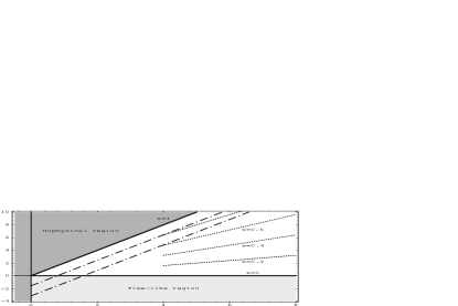
Refer to caption

Figure 3: $(\nu,Q^{2})$ plane. Units in $GeV^{2}.$ Unshaded region is the domain of the structure functions. Solid lines are for $x=$ 0, 0.2, 0.4, 0.6, 0.8 and 1.0. Dashed lines are for $M_{R}^{2}=$ 1.6 and 3.2 $GeV^{2}.$

The scaling region for nucleons is the region above $Q^{2}\sim 1$ GeV. It is described by perturbative QCD. The relevant degrees of freedom are quarks and gluons, and the structure functions are described in terms of quark distribution functions, which depend only on $x$ if we neglect logarithmic deviations. In this approximation, the structure functions are constant along the constant-$x$ lines.

The resonance region in the $(\nu,Q^{2})$ plane is described by the two dashed lines parallel to the elastic or $x=1$ line. These lines satisfy the equation for constant squared invariant mass of intermediate resonant states,

$$M_{R}^{2}=(p+q)^{2}=p^{2}+2\nu-Q^{2}\ \ .$$ (33)

Since the graph is for pion values we choose the $a_{1}$ as the first resonance, $m_{a_{1}}=1.26$ GeV. We also include a second resonance with mass $m_{R}=\sqrt{2}\>m_{a_{1}}$ in order to show the position of possible higher resonances.

This resonance region is described by chiral Lagrangians which include spin-1 resonances such as Eq. (19), [24, 25]. The structure functions obtained through the chiral Lagrangians in the narrow-width approximation are constrained to the elastic line, the $a_{1}$ line, plus other parallel lines corresponding to possible higher resonances. If we include a finite width for the resonances, these lines become bands whose thickness is proportional to the resonance width.

The usefulness of applying the Cottingham method arises from the breakdown of the scattering amplitude into the three terms shown in Eq. (31). We gain control because we can make reasonable assumptions and establish constraints on the pion structure functions. At the same time, it is possible to relate the subtraction term to the soft-pion limit.

All of the resonances couplings will contain form-factors which suppress the effect of an individual resonance as $Q^{2}\to\infty$. We will assume that the fall-off of all such photon form-factors will involve a scale which is a typical vector meson mass. We now turn to the procedure to introduce these form-factors in our dispersive framework. This has a subtlety in that some naive structures for this form-factor could upset the soft-pion limits in our formulas. We will chose a form which is well behaved in the soft-pion limit. The form-factor also solves what would appear to be a problem in the present inclusion of resonances, i.e. the structure function $W_{1}(Q^{2},\nu)$ given in Eq. (31) has terms proportional to $\nu^{2}$ and $Q^{4}$ which would generate divergences for large $Q^{2}$. This is does not occur in the presence of the form-factors. This divergent behavior is clear if we calculate $W_{1}(Q^{2},\nu)$ along the lines of constant $s=m_{R}^{2}\>$. We use the delta function to eliminate the $\nu$ dependence, i.e., $\nu={{1}\over{2}}(s-p^{2}+Q^{2})\>$, to obtain

$$W_{1}^{(cst\>s)}(Q^{2},\nu)={{1}\over{F_{\pi}^{2}}}{{\rho^{R}_{A}(s)}\over{s}}\>{{1}\over{4}}\>(s-p^{2}-Q^{2})^{2}\ \ ,$$ (34)

which diverges as $Q^{4}$. A structure function for a given resonant state cannot diverge for large $Q^{2}$ without violating unitarity. For a single resonance, as it is the case in question, the structure function must go to zero if we follow a line of constant invariant mass, $s$, to high energies. In order to achieve this behavior, we introduce a multiplicative factor which forces its convergence. This factor, $K(\nu,s)$ resembles the form factor obtained for the elastic term through the vector meson dominance model. In addition, it has the following properties,

$\displaystyle\displaystyle K(\nu=0,s)$ $\displaystyle\displaystyle=$ $\displaystyle\displaystyle 1\ \ ,$
$\displaystyle\displaystyle\lim_{Q^{2}\rightarrow\infty}K(\nu,s)^{(cst.\>s)}$ $\displaystyle\displaystyle\sim$ $\displaystyle\displaystyle{{1}\over{Q^{6}}}\ \ ,$
$\displaystyle\displaystyle\left[K(\nu,s)^{(cst.\>s)}\right]_{Q^{2}=0}$ $\displaystyle\displaystyle=$ $\displaystyle\displaystyle 1\ \ .$ (35)

These properties ensure that the subtraction term is left unchanged, and that the structure function will converge for large $Q^{2}.$ The form factor is normalized in order to agree with the previous result at $Q^{2}=0$ for fixed s. The form factor that satisfies these conditions is

$$K(\nu,s)=\left({{m_{V}^{2}}\over{m_{V}^{2}+2\nu}}\right)^{4}\left(1+\eta{{2\nu}\over{s}}\right)\ \ ,$$ (36)

where

$$\eta={{s}\over{s-p^{2}}}\left[\left(1+{{s-p^{2}}\over{m_{V}^{2}}}\right)^{4}-1\right]\ \ ,$$ (37)

and $p^{2}=m_{\pi}^{2}\,.$ We have chosen the appropriate value for the vector meson mass, $m_{V}=m_{\rho}\,.$ The factor $K(\nu,s)$ above, also has the property of being very close to the $\rho$ contribution to the pion EM form factor for $s=p^{2},$ as it can be seen in Fig. 4.

Refer to caption

Figure 4: Factor $K(\nu,s)$ and pion EM form factor. Pion EM form factor, solid line. $K(\nu,m_{\pi}^{2}),$ dashed line. $K(\nu,1\ \mbox{GeV}^{2})$, dash-dotted line. $K(\nu,2\ \mbox{GeV}^{2})$, dotted line. Horizontal scale represents $Q^{2}$ in $\mbox{GeV}^{2}.$

The inclusion of this factor in our analysis is easily achieved through the substitution

$$\rho^{R}_{A}(s)\to\rho^{R}_{A}(s)\>K(\nu,s)\ \ .$$ (38)

The structure functions and subtraction terms read

$\displaystyle\displaystyle T_{1}(-Q^{2},0)$ $\displaystyle\displaystyle=$ $\displaystyle\displaystyle-2+{{2}\over{F_{\pi}^{2}}}\int_{0}^{\infty}\!\!ds\rho^{R}_{V}(s){{Q^{2}}\over{s+Q^{2}}}$
$\displaystyle\displaystyle-{{2}\over{F_{\pi}^{2}}}\int_{0}^{\infty}\!\!ds\rho^{R}_{A}(s){{Q^{2}}\over{s-p^{2}+Q^{2}}}\left(1-{{p^{2}}\over{s}}\right)\ \ ,$
$\displaystyle\displaystyle W_{1}(-Q^{2},\nu)$ $\displaystyle\displaystyle=$ $\displaystyle\displaystyle{{1}\over{F_{\pi}^{2}}}\int_{0}^{\infty}\!\!ds{{\rho^{R}_{A}(s)}\over{s}}\>K(\nu,s)\>(\nu-Q^{2})^{2}\>\delta(s-p^{2}+Q^{2}-2\nu)\ \ ,$
$\displaystyle\displaystyle W_{2}(-Q^{2},\nu)$ $\displaystyle\displaystyle=$ $\displaystyle\displaystyle 4m_{\pi}^{2}\left({{m_{\rho}^{2}}\over{m_{\rho}^{2}+Q^{2}}}\right)^{2}\delta(Q^{2}-2\nu)$ (39)
$\displaystyle\displaystyle+{{1}\over{F_{\pi}^{2}}}\int_{0}^{\infty}\!\!ds{{\rho^{R}_{A}(s)}\over{s}}\>K(\nu,s)\>p^{2}Q^{2}\>\delta(s-p^{2}+Q^{2}-2\nu)\ \ .$

The pion EM mass difference for the above functions is readily obtained with Eq. (17). We choose to break it into terms corresponding to those shown in the above equation with an extra subdivision of the $W_{2}$ contribution which isolates the elastic term

$\displaystyle\displaystyle\Delta m_{\pi}^{2}(Subtr.)$ $\displaystyle\displaystyle=$ $\displaystyle\displaystyle{{\alpha}\over{4\pi}}\int_{0}^{\infty}\!dQ^{2}{{3}\over{F_{\pi}^{2}}}\left[F_{\pi}^{2}-\int_{0}^{\infty}\!\!ds\rho^{R}_{V}(s){{Q^{2}}\over{s+Q^{2}}}\right.$
$\displaystyle\displaystyle\left.\qquad\qquad\ +\int_{0}^{\infty}\!\!ds\rho^{R}_{A}(s){{Q^{2}}\over{s-p^{2}+Q^{2}}}\left(1-{{p^{2}}\over{s}}\right)\right]\ \ ,$
$\displaystyle\displaystyle\Delta m_{\pi}^{2}(W_{1})$ $\displaystyle\displaystyle=$ $\displaystyle\displaystyle{{\alpha}\over{4\pi}}\int_{0}^{\infty}\!dQ^{2}{{6}\over{F_{\pi}^{2}}}\int_{0}^{\infty}\!\!ds{{\rho^{R}_{A}(s)}\over{s}}{{1}\over{\Delta^{2}}}\left({{\Delta^{2}}\over{2}}-Q^{2}\right)^{2}\Lambda_{1}\!\left({{\Delta^{4}}\over{4p^{2}Q^{2}}}\right)K\left({{\Delta^{2}}\over{2}},s\right)\ \ ,$
$\displaystyle\displaystyle\Delta m_{\pi}^{2}(Elast.)$ $\displaystyle\displaystyle=$ $\displaystyle\displaystyle{{\alpha}\over{4\pi}}\int_{0}^{\infty}\!dQ^{2}\left({{m_{\rho}^{2}}\over{m_{\rho}^{2}+Q^{2}}}\right)^{2}\ \Lambda_{2}\!\left({{Q^{2}}\over{4p^{2}}}\right)\ \ ,$
$\displaystyle\displaystyle\Delta m_{\pi}^{2}(W_{2})$ $\displaystyle\displaystyle=$ $\displaystyle\displaystyle{{\alpha}\over{4\pi}}\int_{0}^{\infty}\!dQ^{2}{{1}\over{2F_{\pi}^{2}}}\int_{0}^{\infty}\!\!ds{{\rho^{R}_{A}(s)}\over{s}}\>\Delta^{2}\>\Lambda_{2}\!\left({{\Delta^{4}}\over{4p^{2}Q^{2}}}\right)K\left({{\Delta^{2}}\over{2}},s\right)\ \ ,$ (40)

where $\Delta^{2}=s-p^{2}+Q^{2},$ and $\Lambda_{i}(y)$ (for $i=1,2$ ) are defined in Eq. (18).


High energy constraints

Even though, we can obtain an explicit formula for the pion EM mass difference by adding all the contributions in Eqs. (40), it is necessary to analyze the upper limit of the $Q^{2}$ integral. Adding all the different contributions in Eqs. (40), and expanding the $Q^{2}$ integrand in powers of $1/Q^{2n}$, we obtain,

$\displaystyle\displaystyle-$ $\displaystyle\displaystyle\left({{3\alpha}\over{4\pi F_{\pi}^{2}}}\right)\left[-F_{\pi}^{2}+\int_{0}^{\infty}\!\!ds\left[\rho^{R}_{V}(s)-\rho^{R}_{A}(s)\left(1-{{p^{2}}\over{s}}\right)\right]\right]\ {{1}\over{Q^{0}}}$ (41)
$\displaystyle\displaystyle+$ $\displaystyle\displaystyle\left({{3\alpha}\over{4\pi F_{\pi}^{2}}}\right)\int_{0}^{\infty}\!\!ds\,s\left[\rho^{R}_{V}(s)-\rho^{R}_{A}(s)\left(1-{{p^{2}}\over{s}}\right)^{2}\right]\ {{1}\over{Q^{2}}}\ +\ {\cal O}\left({{1}\over{Q^{4}}}\right)\ \ ,$

where, $p^{2}=m_{\pi}^{2}$. If the first two terms are not zero, they originate linear and logarithmic divergences respectively. In order to obtain a finite pion EM mass difference we cancel them explicitly generating two constraint equations,

$\displaystyle\displaystyle\int_{0}^{\infty}\!\!ds\left[\rho^{R}_{V}(s)-\rho^{R}_{A}(s)\left(1-{{p^{2}}\over{s}}\right)\right]$ $\displaystyle\displaystyle=$ $\displaystyle\displaystyle F_{\pi}^{2}\ \ ,$ (42)
$\displaystyle\displaystyle\int_{0}^{\infty}\!\!ds\,s\left[\rho^{R}_{V}(s)-\rho^{R}_{A}(s)\left(1-2{{p^{2}}\over{s}}+{{p^{4}}\over{s^{2}}}\right)\right]$ $\displaystyle\displaystyle=$ $\displaystyle\displaystyle 0\ \ .$ (43)

These high $Q^{2}$ constraints become the Weinberg sum rules in the soft pion limit, which in the above equations is obtained by letting $p^{2}=0$. We will see later a more detailed explanation of this limit and its relation to the subtraction term.

Due to the introduction of the convergence factor $K(\nu,s)$, the above divergences originate only from the subtraction term. We incorporate the high $Q^{2}$ constraints in the subtraction term of the pion EM mass difference Eq. (40) in order to make all the contributions finite. The following procedure removes both divergences.

Subtract the linear divergence from the subtraction term by means of Eq. (42),

$\displaystyle\displaystyle\Delta m_{\pi}^{2}(Subtr.)$ $\displaystyle\displaystyle=$ $\displaystyle\displaystyle{{\alpha}\over{4\pi}}\int_{0}^{\infty}dQ^{2}{{3}\over{F_{\pi}^{2}}}\left\{F_{\pi}^{2}-\int_{0}^{\infty}\!\!ds\rho^{R}_{V}(s){{Q^{2}}\over{s+Q^{2}}}\right.$ (44)
$\displaystyle\displaystyle+\int_{0}^{\infty}\!\!ds\rho^{R}_{A}(s){{Q^{2}}\over{s-p^{2}+Q^{2}}}\left(1-{{p^{2}}\over{s}}\right)$
$\displaystyle\displaystyle\left.-\left[F_{\pi}^{2}-\int_{0}^{\infty}\!\!ds\rho^{R}_{V}(s)+\int_{0}^{\infty}\!\!ds\rho^{R}_{A}(s)\left(1-{{p^{2}}\over{s}}\right)\right]\right\}$
$\displaystyle\displaystyle=$ $\displaystyle\displaystyle{{\alpha}\over{4\pi}}\int_{0}^{\infty}dQ^{2}{{3}\over{F_{\pi}^{2}}}\left\{\int_{0}^{\infty}\!\!ds\rho^{R}_{V}(s){{s}\over{s+Q^{2}}}\right.$
$\displaystyle\displaystyle\left.-\int_{0}^{\infty}\!\!ds\rho^{R}_{A}(s){{s-p^{2}}\over{s-p^{2}+Q^{2}}}\left(1-{{p^{2}}\over{s}}\right)\right\}\ \ .$

Integrate over $Q^{2}$ and cancel the correspondent logarithmic divergence by subtracting Eq. (43) multiplied by ln $\Lambda_{Q^{2}}$ ,

$$\begin{array}[]{l}\Delta m_{\pi}^{2}(Subtr.)=\\ \\ \qquad\lim_{\Lambda_{Q^{2}}\rightarrow\infty}{{\alpha}\over{4\pi}}{{3}\over{F_{\pi}^{2}}}\left\{\int_{0}^{\infty}\!\!dss\rho^{R}_{V}(s)\ln{{\Lambda_{Q^{2}}+s}\over{s}}\right.\\ \\ \qquad-\int_{0}^{\infty}\!\!ds\rho^{R}_{A}(s)(s-p^{2})\left(1-{{p^{2}}\over{s}}\right)\ln{{\Lambda_{Q^{2}}+s-p^{2}}\over{s-p^{2}}}\\ \\ \qquad-\left.\left[\int_{0}^{\infty}\!\!dss\rho^{R}_{V}(s)\ln\Lambda_{Q^{2}}-\int_{0}^{\infty}\!\!ds\rho^{R}_{A}(s)(s-p^{2})^{2}\ln\Lambda_{Q^{2}}\right]\right\}\ \ .\end{array}$$ (45)

Add the terms and take the limit $\Lambda_{Q^{2}}\rightarrow\infty,$ to obtain

$$\begin{array}[]{l}\Delta m_{\pi}^{2}(Subtr.)=\\ \\ \qquad-{{\alpha}\over{4\pi}}{{3}\over{F_{\pi}^{2}}}\int_{0}^{\infty}\!\!ds\left[s\ln s\ \rho^{R}_{V}(s)-(s-p^{2})\ln(s-p^{2})\rho^{R}_{A}(s)\left(1-{{p^{2}}\over{s}}\right)\right]\ \ .\end{array}$$ (46)

The above contribution is free of divergences. Furthermore, in the soft-pion limit, i.e. $p^{2}=0$, it is equivalent to the Das et al. calculation [21]. Finally, we have a useful formula to calculate $\delta m_{\pi}^{(EM)}$ free of divergences, which was mainly the product of the Lagrangian introducing the chiral couplings of the spin-1 resonances. We proceed to show the close relation of the subtraction term and the soft-pion limit and to see how we reproduce the results of ${\cal O}(p^{4})$ chiral perturbation theory with the above scattering amplitude.


Soft-pion limit and its relation to the subtraction term

In the following we will show that the subtraction term is given by the soft-pion limit up to corrections of order $p^{2}$. In this discussion we refer to non-contact contributions as all contributions except the pion seagull term. This term is the only one which has both photons interacting at the same vertex and therefore we treat it differently in the following discussion.

The non-contact contributions to the Compton scattering amplitude have the form

$$T^{(NC)}_{\mu\nu}(q^{2},p\!\cdot\!q)=i\int\!\!dxe^{-iqx}\langle\pi|T\left(V_{\mu}(x)V_{\nu}(0)\right)|\pi\rangle\ \ .$$ (47)

Consider the soft-pion theorem [29],

$$\lim_{p_{\mu}\rightarrow 0}\langle\pi^{k}(p)\beta|O|\alpha\rangle=-{{i}\over{F_{\pi}}}\langle\beta|\left[Q_{5}^{k},O\right]|\alpha\rangle\ \ ,$$ (48)

where $\beta$ and $\alpha$ are arbitrary states and $Q_{5}^{k}=\int\!\!d^{3}xA_{0}^{k}(x)$ is an axial charge. We also need the commutators

$$\left[Q_{5}^{i},V_{\mu}^{j}\right]\ \ =\ \ if^{ijk}V_{\mu}^{k}\ \ ,\qquad\left[Q_{5}^{i},A_{\mu}^{j}\right]\ \ =\ \ if^{ijk}A_{\mu}^{k}\ \ .$$ (49)

The result of applying the soft-pion theorem to Eq. (47) is

$$\lim_{p_{\mu}\rightarrow 0}T^{(NC)}_{\mu\nu}(q^{2},p\!\cdot\!q)=-i\int\!\!d^{4}xe^{iqx}{{-2}\over{F_{\pi}^{2}}}\langle 0|T\left(V_{3}^{\mu}(x)V_{3}^{\nu}(0)-A_{3}^{\mu}(x)A_{3}^{\nu}(0)\right)|0\rangle\ \ .$$ (50)

The two-current time ordered products are related to the spectral functions by

$\displaystyle\displaystyle\langle 0|T\left(V_{a}^{\mu}(x)V_{b}^{\nu}(0)\right)|0\rangle$ $\displaystyle\displaystyle=$ $\displaystyle\displaystyle i\delta_{ab}\int_{0}^{\infty}\!\!ds\rho_{V}(s)\left(\Box g_{\mu\nu}-\partial^{\mu}\partial^{\nu}\right)\int{{d^{4}k}\over{(2\pi)^{4}}}{{e^{-ikx}}\over{k^{2}-s+i\epsilon}}\ \ ,$
$\displaystyle\displaystyle\langle 0|T\left(A_{a}^{\mu}(x)A_{b}^{\nu}(0)\right)|0\rangle$ $\displaystyle\displaystyle=$ $\displaystyle\displaystyle-i\delta_{ab}F_{\pi}^{2}\partial^{\mu}\partial^{\nu}\int{{d^{4}k}\over{(2\pi)^{4}}}{{e^{-ikx}}\over{k^{2}+i\epsilon}}$ (51)
$\displaystyle\displaystyle\!\!\!\!\!\!\!\!\!\!\!\!\!\!\!\!\!\!\!\!\!\!\!\!\!\!\!\!\!\!\!\!\!\!\!\!\!\!\!\!\!\!\!\!\!\!\!\!\!\!+i\delta_{ab}\int_{0}^{\infty}\!\!ds\rho_{A}(s)\left(\Box g_{\mu\nu}-\partial^{\mu}\partial^{\nu}\right)\int{{d^{4}k}\over{(2\pi)^{4}}}{{e^{-ikx}}\over{k^{2}-s+i\epsilon}}\ \ .$

Upon combining Eqs. (50) and (51), integrating over $d^{4}x,$ and using the resulting $\delta$ function to integrate over $d^{4}k$, we obtain

$$\begin{array}[]{l}\lim_{p_{\mu}\rightarrow 0}T^{(NC)}_{\mu\nu}(q^{2},p\!\cdot\!q)\ \ =\\ \\ \qquad-2{{q^{\mu}q^{\nu}}\over{q^{2}+i\epsilon}}+{{2}\over{F_{\pi}^{2}}}\int_{0}^{\infty}\!\!ds\left(-g^{\mu\nu}+{{q^{\mu}q^{\nu}}\over{q^{2}}}\right)\left(\rho_{V}(s)-\rho_{A}(s)\right){{q^{2}}\over{q^{2}-s+i\epsilon}}\ \ .\end{array}$$ (52)

The contact term or pion seagull contribution to the pion Compton scattering amplitude is

$$T^{(C)}_{\mu\nu}(q^{2},p\!\cdot\!q)=2g_{\mu\nu}\ \ ,$$ (53)

which remains unchanged in the soft-pion limit. Adding both contributions to the pion Compton scattering amplitude in the soft-pion limit, we obtain

$$\lim_{p_{\mu}\rightarrow 0}T_{\mu\nu}(q^{2},p\!\cdot\!q)=D_{1_{\mu\nu}}\left\{-2+{{2}\over{F_{\pi}^{2}}}\int_{0}^{\infty}\!\!ds(\rho_{V}(s)-\rho_{A}(s)){{q^{2}}\over{q^{2}-s}}\right\}\ \ .$$ (54)

An alternative way of reproducing the soft-pion limit result above, is letting $p_{\mu}\rightarrow 0$ in Eq. (29). In order to implement this limit the following relations are useful,

$\displaystyle\displaystyle\lim_{p_{\mu}\rightarrow 0}D_{1_{\mu\nu}}$ $\displaystyle\displaystyle=$ $\displaystyle\displaystyle D_{1_{\mu\nu}}\ \ ,$
$\displaystyle\displaystyle\lim_{p_{\mu}\rightarrow 0}p^{2}D_{2_{\mu\nu}}$ $\displaystyle\displaystyle=$ $\displaystyle\displaystyle 0\ \ ,$
$\displaystyle\displaystyle\lim_{p_{\mu}\rightarrow 0}T_{1}(q^{2},p\!\cdot\!q)$ $\displaystyle\displaystyle=$ $\displaystyle\displaystyle\left.T_{1}(q^{2},0)\right|_{p^{2}=0}\ \ .$ (55)

From these relations it follows that the only surviving term in this limit is the subtraction term $T_{1}(q^{2},0),$

$$\lim_{p_{\mu}\rightarrow 0}T_{\mu\nu}(q^{2},p\!\cdot\!q)=D_{1_{\mu\nu}}\lim_{p_{\mu}\rightarrow 0}T_{1}(q^{2},0)\ \ .$$ (56)

This gives the same result as Eq. (54) when we identify

$$\lim_{p_{\mu}\rightarrow 0}\left(\rho_{V}^{R}(s)-\rho_{A}^{R}(s)\right)=\left(\rho_{V}(s)-\rho_{A}(s)\right)\ \ .$$ (57)

We can now calculate the soft-pion limit to the pion EM mass difference,

$$\lim_{p_{\mu}\rightarrow 0}\Delta m_{\pi}^{2}={{\alpha}\over{4\pi}}\int_{0}^{\infty}\!\!dQ^{2}{{3}\over{F_{\pi}^{2}}}\left\{F_{\pi}^{2}-\int_{0}^{\infty}\!\!ds\left(\rho_{V}(s)-\rho_{A}(s)\right){{Q^{2}}\over{Q^{2}+s}}\right\}\ \ ,$$ (58)

where $Q^{2}=-q^{2}$. We follow the procedure described earlier in order to cancel the linear and logarithmic divergences occurring in the above equation. The cancellation of these divergences imposed by the finiteness of the pion EM mass difference requires

$\displaystyle\displaystyle\int_{0}^{\infty}\!\!ds\left(\rho_{V}(s)-\rho_{A}(s)\right)$ $\displaystyle\displaystyle=$ $\displaystyle\displaystyle F_{\pi}^{2}\ \ ,$ (59)
$\displaystyle\displaystyle\int_{0}^{\infty}\!\!dss\left(\rho_{V}(s)-\rho_{A}(s)\right)$ $\displaystyle\displaystyle=$ $\displaystyle\displaystyle 0\ \ .$ (60)

These are Weinberg sum rules [22], obtained in our case as a consequence of the finiteness of $\delta m_{\pi}^{(EM)}$ in the soft-pion limit. Subtracting the linear and logarithmic divergences in the same way as for the subtraction term, Eqs. (44-46), we obtain

$$\lim_{p_{\mu}\rightarrow 0}\Delta m_{\pi}^{2}=-{{\alpha}\over{4\pi}}{{3}\over{F_{\pi}^{2}}}\int_{0}^{\infty}\!\!dss\ln s\left(\rho_{V}(s)-\rho_{A}(s)\right)\ \ .$$ (61)

This is the result obtained by Das et al. [21].

Finally, we evaluate Eq. (61) in the narrow-width approximation to obtain the numerical result

$$\lim_{p_{\mu}\rightarrow 0}\Delta m_{\pi}^{(NW)}=4.685\ \mbox{MeV}\ \ .$$ (62)

Spectral functions

We seek an improved description of the physics of the resonance region with the spectral functions $\rho^{R}_{V}(s)$ and $\rho^{R}_{A}(s)$ replacing the narrow-width description. The ingredients to the spectral functions clearly are the same resonance states that are revealed by the usual vector and axial-vector spectral functions $\rho_{V}(s)$ and $\rho_{A}(s)$. In addition we have just seen that in the soft-pion limit there is an exact correspondence $\rho^{R}_{V}(s)-\rho^{R}_{A}(s)=\rho_{V}(s)-\rho_{A}(s)$. This leads us to utilize the experimental spectral functions determined in reference [13] in order to produce a shape for $\rho^{R}_{V}(s)$ and $\rho^{R}_{A}(s)$. In both the soft-pion limit and the full Cottingham calculation at order $m_{\pi}^{2}$, the high energy continuum cancels in the mass shift. We therefore separate each spectral function into two contributions, one due to the resonances and the other due to the high energy continuum common to both vector and axial-vector channels. The resonant part is chosen to match the resonances revealed in the phenomenological analysis of the data in [13]. These spectral functions are then slightly altered to obey the full constraint equations including $p^{2}$ terms of Eqs. (85) and (86). A continuum contribution, common to both vector and axial-vector channels, was included in [13], but is here kept separate from the resonances. The result of this is that we identify

$$\rho_{V,A}(s)=\rho_{V,A}^{R}(s)+\rho_{V,A}^{C}(s)\ \ ,$$ (63)

with a continuum contribution

$$\rho^{C}(s)=\rho_{V}^{C}(s)=\rho_{A}^{C}(s)\ \ .$$ (64)

The precise identification of the continuum is not unique, but since the difference of spectral functions enters, reasonable variations do not produce a large final effect. The specific form that we use is
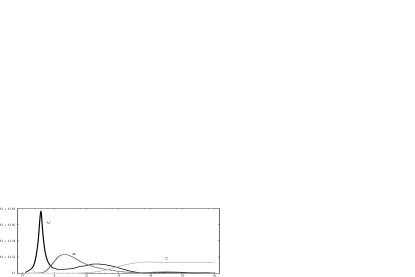
 shown in Fig. 5.

Refer to caption

Figure 5: Vector and axial-vector spectral functions. The graph shows (V) $\rho_{V}^{R}(s),$ (A) $\rho_{A}^{R}(s),$ and (C) $\rho_{C}(s)$ versus $s$. The $s$ scale is given in $\mbox{GeV}^{2}.$

It is clear that the greatest source of model dependence in our calculation comes form the numerical identification described above. Our procedure in setting up the calculation in the Cottingham method is very general. However, we do not have directly available the experimental structure functions for photons scattering off of pions. We have used an identification which is valid in the chiral limit in order to provide this numerical input. There could be shifts in the couplings of these resonances which are of order $m_{\pi}^{2}$. These could provide changes in the final answer at order $m_{\pi}^{2}$ which would be of interest to us. This is partially relieved by the fact that the analysis of [13] was carried out with real world data, not strictly in the chiral limit. Thus the masses, widths and shapes of the resonances will accurately reflect physics with $m_{\pi}^{2}\neq 0$. Likewise we know that in the narrow-width approximation we have the right description, so that we don’t see a source of major uncertainty due to the non-zero widths. This means that our model dependence comes from possible $m_{\pi}^{2}$ dependences in the resonance couplings, and our implicit assumption is that these are smaller than the $m_{\pi}^{2}$ dependence from the propagators. We have not been able to find a way to do better than this in the phenomenological analysis.


Comparison $O(E^{4})$ Chiral Perturbation Theory

We also like to compare our method to the standard chiral perturbation approach. The lowest energy region of the pion structure function can be described by the chiral SU(3) Lagrangian to order $p^{4}$, originally developed by Gasser and Leutwyler [11, 12]. Besides the elastic and seagull terms, and ignoring pion loops, the only relevant terms involved in the pion Compton scattering amplitude are the $L_{9}$ and $L_{10}$ terms,

$\displaystyle\displaystyle{\cal L}_{4}=$ $\displaystyle\displaystyle-$ $\displaystyle\displaystyle iL_{9}\mbox{Tr}\left(F^{\mu\nu}_{R}D_{\mu}UD_{\nu}U^{\dagger}+F^{\mu\nu}_{L}D_{\mu}U^{\dagger}D_{\nu}U\right)$ (65)
$\displaystyle\displaystyle+$ $\displaystyle\displaystyle L_{10}\mbox{Tr}\left(U^{\dagger}F^{\mu\nu}_{R}UF_{L\mu\nu}\right)+\mbox{\ other}\ .$

The pion forward Compton scattering amplitude resulting from this Lagrangian was calculated by Bijnens and Cornet [14], and Donoghue et al. [15]. Their result, up to pion loop contributions which are small, is

$\displaystyle\displaystyle T_{\mu\nu}(p,q)$ $\displaystyle\displaystyle=$ $\displaystyle\displaystyle-{{8p^{2}q^{2}}\over{q^{4}-(2p\!\cdot\!q)^{2}}}\left(1+{{2L_{9}^{r}q^{2}}\over{F_{\pi}^{2}}}\right)^{2}D_{2_{\mu\nu}}$ (66)
$\displaystyle\displaystyle-2D_{1_{\mu\nu}}+{{8L_{10}^{r}q^{2}}\over{F_{\pi}^{2}}}D_{1_{\mu\nu}}+\mbox{\ loops}\ \ ,$

Expanding our narrow-width result in powers of external momenta $p_{\mu}$ and $q_{\mu}$, we obtain,

$$\begin{array}[]{l}T_{\mu\nu}^{(q^{2}\ exp.)}(q^{2},p\!\cdot\!q)\ =\ D_{1_{\mu\nu}}\left\{-2-2{{F_{V}^{2}}\over{F_{\pi}^{2}}}{{q^{2}}\over{m_{\rho}^{2}}}+2{{F_{A}^{2}}\over{F_{\pi}^{2}}}{{q^{2}}\over{m_{A}^{2}}}\right\}\\ \\ \qquad+\ D_{2_{\mu\nu}}\left\{4m_{\pi}^{2}\left(1+{{q^{2}}\over{m_{V}^{2}}}\right)^{2}{{-2q^{2}}\over{q^{4}-(2p\!\cdot\!q)^{2}}}\ +2{{F_{A}^{2}}\over{F_{\pi}^{2}m_{A}^{2}}}{{-m_{\pi}^{2}q^{2}}\over{m_{A}^{2}}}\right\}\\ \\ \qquad+\ \mbox{higher order terms in }(q^{2},p\!\cdot\!q,p^{2})\ \ .\end{array}$$ (67)

The relations for the $L_{9}$ and $L_{10}$ in terms of the spin-1 resonance parameters are obtained by inspection from Eqs. (66) and (67).

$\displaystyle\displaystyle L_{9}$ $\displaystyle\displaystyle=$ $\displaystyle\displaystyle{{F_{\pi}^{2}}\over{2m_{V}^{2}}}\ \ ,$
$\displaystyle\displaystyle L_{10}$ $\displaystyle\displaystyle=$ $\displaystyle\displaystyle-{{1}\over{4}}\left({{F_{V}^{2}}\over{m_{V}^{2}}}-{{F_{A}^{2}}\over{2m_{A}^{2}}}\right)\ \ .$ (68)

This result is in agreement with Ecker et al. [24]. The above equation for $L_{10}$ is also the narrow-width approximation for the sum rule (W0) in reference [13]

Substituting the narrow-width parameters in Eq. (68) we obtain,

$\displaystyle\displaystyle L_{9}$ $\displaystyle\displaystyle=$ $\displaystyle\displaystyle(7.20\pm 0.05)\times 10^{-3}\ \ ,$
$\displaystyle\displaystyle L_{10}$ $\displaystyle\displaystyle=$ $\displaystyle\displaystyle-(5.89\pm 0.65)\times 10^{-3}\ \ .$ (69)

These are seen to be within reasonable agreement with the experimental values,

$\displaystyle\displaystyle L_{9}$ $\displaystyle\displaystyle=$ $\displaystyle\displaystyle(7.1\pm 0.3)\times 10^{-3}\ \ ,$
$\displaystyle\displaystyle L_{10}$ $\displaystyle\displaystyle=$ $\displaystyle\displaystyle-(6.84\pm 0.3)\times 10^{-3}\ \ .$ (70)

The difference between the values in Eq. (69) and (70) gives an estimate for the loop contributions which we neglected in the ${\cal O}(p^{4})$ chiral Lagrangian calculation of the Compton scattering amplitude. Besides the loop corrections, the difference can also be due to the inaccuracy of the narrow-width approximation.


Scaling region

The low and intermediate energy regions of the structure functions are described above. To complete the analysis of the structure functions we need to describe the scaling region at large values of $(\nu,Q^{2})$. The ingredients and general behavior in this region are well known. The structure functions become largely functions of the Bjorken scaling variable $x={Q^{2}}/{2\nu}$, with logarithmic $Q^{2}$ variations predictable by QCD [30]. This is easy to build into the Cottingham analysis [31]. However there is not a need to describe the details here since the scaling region cancels in the difference between the charged and neutral pions masses, to the order that we are working here.

In the limit that the u and d quark masses are equal, the deep inelastic structure functions of the neutral and charged pions are equal. This leads to

$$\Delta m_{\pi}(Scaling)=0\ \ .$$ (71)

To the extent that the u, d masses are different, the structure functions may differ. However we are calculating the electromagnetic effect in the limit $m_{u}=m_{d}$, so that we are not sensitive to this effect.


$V\rightarrow\pi\gamma$ contribution

To have a more complete phenomenological description of the Compton scattering amplitude we also include the effect of intermediate vector meson diagrams shown in Fig. 6. The motivation for introducing these diagrams is the experimental observation of the radiative meson decays $\omega\rightarrow\pi\gamma$ and $\rho\rightarrow\pi\gamma,$ and $\phi\rightarrow\pi\gamma.$ The effective Lagrangian which includes the $V\pi\gamma$ vertices is

$${\cal L}=e{{\sqrt{R_{V}}}\over{2}}\epsilon^{\mu\nu\alpha\beta}F_{\mu\nu}V_{\alpha}\partial_{\beta}\pi\ \ ,$$ (72)

This Lagrangian is invariant under parity and charge conjugation transformations, as well as under chiral rotations. The choice of including the EM field strength tensor ensures gauge invariance, and the pion momentum dependence corresponds to the correct soft-pion limit for the vertex.

\Line(30,50)(85,50) \Vertex(85,50)3 \Line(85,52)(140,52) \Line(85,48)(140,48) \Vertex(140,50)3 \Line(140,50)(195,50) \Photon(30,100)(85,50)3 6 \Photon(140,50)(195,100)3 6 \Line(230,50)(285,50) \Vertex(285,50)3 \Line(285,52)(340,52) \Line(285,48)(340,48) \Vertex(340,50)3 \Line(340,50)(395,50) \Photon(230,100)(340,50)3 9 \Photon(285,50)(395,100)3 9 $\pi$ $\pi$V$\gamma$ $\gamma$ $\pi$ $\pi$V$\gamma$ $\gamma$
Figure 6: Intermediate vector diagrams.

We introduce the spectral functions $g_{V}(s)$ to describe the intermediate states in Fig. 6. The normalization of these functions is chosen in order to make the subtraction term contribution compatible with the ones obtained for the axial-vector case. The narrow-width approximation for $g_{V}(s)$ is

$$g_{V}(s)\ =\ H_{V}^{2}\delta(s-m_{V}^{2})\ =\ F_{\pi}^{2}R_{V}\delta(s-m_{V}^{2})\ \ .$$ (73)

The subtraction term and the structure functions for the intermediate vector meson diagrams follow from the Lagrangian in Eq. (72),

$\displaystyle\displaystyle T_{1}(-Q^{2},0)$ $\displaystyle\displaystyle=$ $\displaystyle\displaystyle{{2}\over{F_{\pi}^{2}}}\int_{0}^{\infty}\!\!dsg_{V}(s){{p^{2}Q^{2}}\over{s-p^{2}+Q^{2}}}\ \ ,$
$\displaystyle\displaystyle W_{1}(-Q^{2},\nu)$ $\displaystyle\displaystyle=$ $\displaystyle\displaystyle{{1}\over{F_{\pi}^{2}}}\int_{0}^{\infty}\!\!dsg_{V}(s)K(\nu,s)(\nu^{2}+p^{2}Q^{2})\delta(s-p^{2}+Q^{2}-2\nu)\ ,$
$\displaystyle\displaystyle W_{2}(-Q^{2},\nu)$ $\displaystyle\displaystyle=$ $\displaystyle\displaystyle{{1}\over{F_{\pi}^{2}}}\int_{0}^{\infty}\!\!dsg_{V}(s)K(\nu,s)p^{2}Q^{2}\delta(s-p^{2}+Q^{2}-2\nu)\ ,$ (74)

where $K(\nu,s)$ is the factor defined in Eq. (36). The factor $K(\nu,s)$ ensures the $Q^{2}$ convergence of the structure functions as in the intermediate axial-vector state case. We only need to find the spectral function $g_{V}(s)$ in order to determine the above functions.

There are four possible vector intermediate states for the pion Compton amplitude, the $\rho^{\pm}$ for the charged pions, and the $\rho^{0}$, $\omega$ and $\phi$ for the neutral pion. The coupling constants, $R_{\rho^{\pm}},$ $R_{\rho^{0}},$ $R_{\omega},$ and $R_{\phi}$ can be extracted from the radiative decays of these vector mesons. We refer the reader to references [17, 23, 32, 33] for a review and examples of obtaining such couplings. The couplings $R_{\rho^{\pm}}$ and $R_{\rho^{0}}$ are the same if we take isospin to be an exact symmetry. This means that the charged and neutral pion EM self energies due to the $\rho$ intermediate state would cancel in the pion EM mass difference. However, the $\omega$ and $\phi$ intermediate state contributions do not present such a cancellation. Since isospin breaking effects are generally of small magnitude, we shall neglect the intermediate $\rho$ contribution to the pion EM mass difference.

We can determine the $\omega$ coupling, $R_{\omega}$, from the experimental measurement of the radiative decay $\omega\rightarrow\pi^{0}\gamma,$

$$R_{\omega}\ =\ {{24}\over{\alpha}}{{m_{\omega}^{3}}\over{(m_{\omega}^{2}-m_{\pi}^{2})^{3}}}\ \Gamma_{\omega\rightarrow\pi\gamma}\ =\ 5.40\pm 0.32\ \mbox{GeV}^{-2}\ \ .$$ (75)

Likewise we determine the $\phi$ coupling, $R_{\phi}$,

$$R_{\phi}\ =\ {{24}\over{\alpha}}{{m_{\phi}^{3}}\over{(m_{\phi}^{2}-m_{\pi}^{2})^{3}}}\ \Gamma_{\phi\rightarrow\pi\gamma}\ =\ 0.019\pm 0.002\ \mbox{GeV}^{-2}\ \ ,$$ (76)

where we have used the experimental values listed by the Particle Data Group [34]. We do not consider the $\phi$ vector meson intermediate state further because its coupling is an order of magnitude smaller than the experimental uncertainty of the $\omega$ coupling.

We are now ready to determine the spectral function $g_{V}(s).$ Since the only resonance involved is the $\omega,$ we can safely use the narrow-width approximation of Eq. (73). The width of the $\omega$ is only $1\%$ of its mass. This is in contrast with the $\rho$ and $a_{1}$ resonances for which the widths are $20\%$ and $33\%$ of their mass respectively. In the narrow-width approximation we only need $m_{\omega}$, taken from [34], and $H_{V}$, given by

$$H_{V}\ =\ F_{\pi}\sqrt{R_{V}}\ =\ 0.215\pm 0.013\ \ .$$ (77)

We should be careful when comparing $g_{V}(s)$ to $\rho_{V,A}(s)$ since they have different units. The relationship among these structure functions will become clear in the following subsection.

The intermediate vector meson subtraction term and structure function contributions to the pion EM mass difference are obtained by combining Eq.s (17) and (74),

$\displaystyle\displaystyle\Delta m_{\pi}^{2}(Subtr.)$ $\displaystyle\displaystyle=$ $\displaystyle\displaystyle{{3\alpha}\over{4\pi F_{\pi}^{2}}}\int_{0}^{\infty}\!\!dQ^{2}\int_{0}^{\infty}\!\!dsg_{V}(s){{p^{2}Q^{2}}\over{s-p^{2}+Q^{2}}}\ \ ,$
$\displaystyle\displaystyle\Delta m_{\pi}^{2}(W_{1})$ $\displaystyle\displaystyle=$ $\displaystyle\displaystyle{{-\alpha}\over{4\pi}}\int_{0}^{\infty}\!\!dQ^{2}{{6}\over{F_{\pi}^{2}}}$
$\displaystyle\displaystyle\times$ $\displaystyle\displaystyle\int_{0}^{\infty}\!\!dsg_{V}(s)K\!\left({{\Delta^{2}}\over{2}},s\right){{1}\over{\Delta^{2}}}\left({{\Delta^{4}}\over{4}}+p^{2}Q^{2}\right)\Lambda_{1}\!\left({{\Delta^{4}}\over{4p^{2}Q^{2}}}\right)\ \ ,$
$\displaystyle\displaystyle\Delta m_{\pi}^{2}(W_{2})$ $\displaystyle\displaystyle=$ $\displaystyle\displaystyle{{-\alpha}\over{4\pi}}\int_{0}^{\infty}\!\!dQ^{2}{{1}\over{2F_{\pi}^{2}}}\int_{0}^{\infty}\!\!dsg_{V}(s)K\!\left({{\Delta^{2}}\over{2}},s\right)\Delta^{2}\Lambda_{2}\!\left({{\Delta^{4}}\over{4p^{2}Q^{2}}}\right)\ \ ,$ (78)

where $\Delta^{2}=s-p^{2}+Q^{2}$, $p^{2}=m_{\pi}^{2}$, and the functions $\Lambda_{i}(y),$ for $i=1,2$ are defined in Eq. (18). The extra minus sign appears because the vector intermediate state diagrams contribute to the neutral pion EM self energy.


General treatment of other possible contributions

At this point we have a fairly complete calculation of the pion EM mass difference broken down into different contributions. We have included the spin-1 resonances through their lowest order chiral couplings, the scaling, and the intermediate vector resonance contributions to the pion EM mass difference. By analogy with the nucleon structure functions, we are comfortable with our estimates of the structure function contributions. These are small, and even a factor of two correction would amount to a small correction to the total mass difference. Therefore, we concentrate in the subtraction term contribution estimate.

The subtraction term has been obtained by calculating the pion Compton scattering amplitude with the effective chiral Lagrangian for the vector and axial-vector resonances of Eq. (19) and the effective Lagrangian for the intermediate vector meson contribution of Eq. (72). In general, there could be other possible contributions to the subtraction term. These could be introduced by higher order effective Lagrangians. Their contributions to $\delta m_{\pi}^{EM}$ would be small since they would be of higher order in the external momenta $p^{2}$ and $q^{2}.$ The terms with higher powers of $p^{2}$ are naturally small, otherwise terms of higher order in $q^{2}$ are in principle divergent. The finiteness of $\delta m_{\pi}^{EM}$ requires that all the higher powers of $q^{2}$ cancel in the same way that the order 1 and $1/Q^{2}$ cancel due to the Weinberg sum rules in the soft-pion limit case.

We include all other possible contributions to the subtraction term, not yet accounted for in the previous analysis, by introducing the remainder term,

$${{2}\over{F_{\pi}^{2}}}\int_{0}^{\infty}\!\!ds\>R(Q^{2},p^{2},s)\ \ .$$ (79)

The purpose of including this term is to show explicitly the effect of possible corrections to our current scattering amplitude and its role in the high energy constraints and final formula for the EM mass difference.

There are some conditions required upon this remainder term. It cannot alter our previous soft-pion limit result, therefore,

$$\lim_{p_{\mu}\rightarrow 0}\int_{0}^{\infty}dsR(Q^{2},p^{2},s)=0\ \ .$$ (80)

It is also convenient to use the following notation for its expansion in powers of $1/Q^{2},$

$$R(Q^{2},p^{2},s)=p^{2}h_{1}(p^{2},s)+{{p^{2}h_{2}(p^{2},s)}\over{Q^{2}+f(p^{2},s)}}+{\cal O}\left({{1}\over{Q^{4}}}\right)\ \ .$$ (81)

We have explicitly introduced a factor of $p^{2}$ in order to make sure that this term vanishes in the soft-pion limit as given in Eq. (80). This limit also requires that the functions $h_{i}(p^{2},s)$ (for $i=1,2$) do not have a pole at $p^{2}=0.$ The above equation is not a formal expansion in orders of $1/Q^{2}$ since we have introduced the function $f(p^{2},s)$ in the denominator of the second term. This has been done in order to make the $Q^{2}$ integral of this term convergent at low $Q^{2}.$ The reason for choosing the above notation will be clear in the following extraction of the subtraction term contribution to $\delta m_{\pi}^{EM}.$

We rewrite the subtraction term contribution,

$$\Delta m_{\pi}^{2}(Subtr.)={{-3\alpha}\over{8\pi}}\int_{0}^{\infty}\!\!dQ^{2}T_{1}(-Q^{2},0)\ \ .$$ (82)

The subtraction term including the remainder part, except its ${\cal O}(1/Q^{4})$ contributions not present in $h_{2}$, is

$$\begin{array}[]{l}T_{1}(-Q^{2},0)\ \ =\ \ -2+{{2}\over{F_{\pi}^{2}}}\int_{0}^{\infty}\!\!ds\left\{\rho^{R}_{V}(s){{Q^{2}}\over{s+Q^{2}}}\right.\\ \\ \qquad-\rho^{R}_{A}(s){{Q^{2}}\over{s-p^{2}+Q^{2}}}\left(1-{{p^{2}}\over{s}}\right)-g_{V}(s){{p^{2}Q^{2}}\over{s-p^{2}+Q^{2}}}\\ \\ \qquad\left.+p^{2}h_{1}(p^{2},s)+{{p^{2}h_{2}(p^{2},s)}\over{Q^{2}+f(p^{2},s)}}\right\}\ \ .\end{array}$$ (83)

We expand the above equation in powers of $1/Q^{2}$ in order to obtain

$$\begin{array}[]{l}T_{1}(-Q^{2},0)\ \ =\\ \\ \ -2+{{2}\over{F_{\pi}^{2}}}\int_{0}^{\infty}\!\!ds\left[\rho^{R}_{V}(s)-{{s-p^{2}}\over{s}}\rho^{R}_{A}(s)-p^{2}g_{V}(s)+p^{2}h_{1}(p^{2},s)\right]\\ \\ \ +\int_{0}^{\infty}\!\!ds\left[s\rho^{R}_{V}(s)-{{(s-p^{2})^{2}}\over{s}}\rho^{R}_{A}(s)-p^{2}(s-p^{2})g_{V}(s)+p^{2}h_{2}(p^{2},s)\right]{{1}\over{Q^{2}}}\\ \\ \ +{\cal O}\left({{1}\over{Q^{4}}}\right)\ \ .\end{array}$$ (84)

The finiteness of $\delta m_{\pi}^{2}$ requires the cancellation of the linear and logarithmic divergences, resulting in the constraints,

$\displaystyle\displaystyle\int_{0}^{\infty}\!\!ds\left\{\left[\rho^{R}_{V}(s)-\rho^{R}_{A}(s)\right]+p^{2}\left[{{\rho^{R}_{A}(s)}\over{s}}-g_{v}(s)+h_{1}(p^{2},s)\right]\right\}$ $\displaystyle\displaystyle=$ $\displaystyle\displaystyle F_{\pi}^{2}\ \ ,$ (85)
$\displaystyle\displaystyle\int_{0}^{\infty}\!\!ds\left\{\left[s\rho^{R}_{V}(s)-s\rho^{R}_{A}(s)\right]\phantom{+p^{2}\left[g_{V}(s)-{{\rho^{R}_{A}(s)}\over{s}}\right]+p^{2}h_{2}(p^{2},s)}\right.$
$\displaystyle\displaystyle\left.+p^{2}\left[2\rho^{R}_{A}(s)-sg_{V}(s)\right]+p^{4}\left[g_{V}(s)-{{\rho^{R}_{A}(s)}\over{s}}\right]+p^{2}h_{2}(p^{2},s)\right\}$ $\displaystyle\displaystyle=$ $\displaystyle\displaystyle 0\ \ .$ (86)

These constraints also reduce to the Weinberg sum rules when we let $p^{2}=0.$ The role of the functions $h_{i}(p^{2},s)$ (for i = 1, 2) is to include all other possible contributions. The above constraints must be satisfied exactly, otherwise the pion EM mass difference would be divergent.

We can use the Weinberg sum rules, Eqs. (59) and (60), to further simplify the previous equations,

$\displaystyle\displaystyle p^{2}\int_{0}^{\infty}\!\!ds\left[{{\rho^{R}_{A}(s)}\over{s}}-g_{v}(s)+h_{1}(p^{2},s)\right]$ $\displaystyle\displaystyle=$ $\displaystyle\displaystyle 0\ ,$ (87)
$\displaystyle\displaystyle p^{2}\int_{0}^{\infty}\!\!ds\left\{\left[2\rho^{R}_{A}(s)-sg_{V}(s)\right]+p^{2}\left[g_{V}(s)-{{\rho^{R}_{A}(s)}\over{s}}\right]+h_{2}(p^{2},s)\right\}$ $\displaystyle\displaystyle=$ $\displaystyle\displaystyle 0\ .$ (88)

We can use solutions available for the functions $\rho^{R}_{A}(s)$ [13] and $g_{V}(s)$ to estimate the integrals for the remainder terms,

$\displaystyle\displaystyle\int_{0}^{\infty}\!\!dsp^{2}h_{1}(p^{2},s)$ $\displaystyle\displaystyle=$ $\displaystyle\displaystyle\int_{0}^{\infty}\!\!dsp^{2}\left[g_{v}(s)-{{\rho^{R}_{A}(s)}\over{s}}\right]$ (89)
$\displaystyle\displaystyle=$ $\displaystyle\displaystyle 3.0\times 10^{-4}\ \ ,$
$\displaystyle\displaystyle\int_{0}^{\infty}\!\!dsp^{2}h_{2}(p^{2},s)$ $\displaystyle\displaystyle=$ $\displaystyle\displaystyle\int_{0}^{\infty}\!\!ds\left\{p^{2}\left[2\rho^{R}_{A}(s)-sg_{V}(s)\right]+p^{4}\left[g_{V}(s)-{{\rho^{R}_{A}(s)}\over{s}}\right]\right\}$ (90)
$\displaystyle\displaystyle=$ $\displaystyle\displaystyle 6.1\times 10^{-4}\ \ .$

As expected, these values are small when compared to the integrals involving $\rho^{R}_{V}(s)$ which are the larger terms in the constraint equations,

$\displaystyle\displaystyle\int_{0}^{\infty}\!\!ds\rho_{V}^{R}(s)$ $\displaystyle\displaystyle=$ $\displaystyle\displaystyle 3.83\times 10^{-2}\ \ ,$ (91)
$\displaystyle\displaystyle\int_{0}^{\infty}\!\!dss\rho_{V}^{R}(s)$ $\displaystyle\displaystyle=$ $\displaystyle\displaystyle 5.62\times 10^{-2}\ \ ,$ (92)

The remainder term $R(Q^{2},p^{2},s)$ allows us to satisfy the constraints exactly since it introduces a small correction to the previous constraint equations. We can proceed to find the subtraction term contribution by following the steps that we used previously in order to obtain Eqs. (44)-(46)

$$\begin{array}[]{l}\Delta m_{\pi}^{2}(Subtr.)\ \ =\\ \\ \qquad{{-3\alpha}\over{4\pi F_{\pi}^{2}}}\int_{0}^{\infty}\!\!ds\left\{\rho^{R}_{V}(s)s\ln s-\rho^{R}_{A}(s){{(s-p^{2})^{2}}\over{s}}\ln\left(s-p^{2}\right)\right.\\ \\ \qquad\left.-g_{V}(s)p^{2}(s-p^{2})\ln\left(s-p^{2}\right)+p^{2}h_{2}(p^{2},s)\ln f(p^{2},s)\!\!\!\phantom{{{1}\over{1}}}\right\}\ \ .\end{array}$$ (93)

Even though the functions $f(p^{2},s)$ and $h_{2}(p^{2},s)$ are undetermined, we have seen in equation (90) that their contributions to the constraint Eq. (86) are small.


Numerical result

The total pion electromagnetic mass difference is given by the addition of the elastic term of Eqs. (40), the structure function terms of Eqs. (40) and (78), and the subtraction constant term of Eq. (93). The results for the narrow-width approximation and for the corresponding spectral functions is given in Table 1.

Table 1: $\Delta m_{\pi}^{EM}$ results.
Narrow-width $\rho_{A}^{R}(s),\rho_{V}^{R}(s)$
(MeV) (MeV)
Subtr. 00004 . 306 0000 4 . 124
Elastic 0 . 500 0 . 500
Str. Fn. $a_{1}$ int. st. 0 . 028 0 . 041
Str. Fn. $\omega$ int. st. -0 . 127 -0 . 127
Total calculated 4 . 707 4 . 538
Experiment 4 . 594 4 . 594

We see from the results that the dominant contribution comes from the subtraction term, which is largely the effect of vector and axial-vector resonances, with modest dependence on $p^{2}=m_{\pi}^{2}$. The elastic term gives the only other significant contribution. The modification due to non-zero width is also not large. The overall result is in excellent agreement with experiment.


5. The kaon EM mass difference


Having set up and tested our methodology for the pion, we now proceed to the calculation of the kaon electromagnetic mass difference. The most important effect is that the larger mass of the kaon leads to kinematic corrections in the various formulae. There are also changes in the mass, width and couplings of the resonances which we extract from the data

The kaon calculation is very similar to the pion one described in the previous section, therefore we will concentrate on the differences that arise in the kaon case. The kaon counterpart for the Lagrangian of Eq. (20) expanded in terms of kaon, photon, and spin-1 resonance fields is

$\displaystyle\displaystyle{\cal L}$ $\displaystyle\displaystyle=$ $\displaystyle\displaystyle ieA^{\mu}(K^{+}\partial_{\mu}K^{-}-K^{-}\partial_{\mu}K^{+})+e^{2}A^{\mu}A_{\mu}K^{+}K^{-}\ \ ,$ (94)
$\displaystyle\displaystyle-{{eF_{V}}\over{2}}F^{\mu\nu}\left(\rho_{\mu\nu}^{0}+{{\sqrt{2}}\over{3}}\phi_{\mu\nu}+{{1}\over{3}}\omega_{\mu\nu}\right)$
$\displaystyle\displaystyle+{{eF_{V}}\over{4F_{K}^{2}}}F^{\mu\nu}\left(\rho_{\mu\nu}^{0}+\sqrt{2}\phi_{\mu\nu}+\omega_{\mu\nu}\right)K^{+}K^{-}$
$\displaystyle\displaystyle+{{iG_{V}}\over{F_{K}^{2}}}\left(\rho_{\mu\nu}^{0}+\sqrt{2}\phi_{\mu\nu}+\omega_{\mu\nu}\right)\partial_{\mu}K^{+}\partial_{\nu}K^{-}$
$\displaystyle\displaystyle+{{iG_{V}}\over{F_{K}^{2}}}\left(-\rho_{\mu\nu}^{0}+\sqrt{2}\phi_{\mu\nu}+\omega_{\mu\nu}\right)\partial_{\mu}K^{0}\partial_{\nu}\overline{K^{0}}\ \ ,$
$\displaystyle\displaystyle-{{ieF_{A}}\over{2F_{K}}}F^{\mu\nu}\left(K_{1_{\mu\nu}}^{-}K^{+}-K_{1_{\mu\nu}}^{+}K^{-}\right)\ \ ,$

where we have used ideal mixing for the vector meson resonances.

The major difference between the kaon and pion Lagrangians - Eqs. (20) and (94) respectively - is that in the kaon case all the three nonet vector resonances contribute. Another difference is that there is an elastic contribution to the neutral kaon self-energy. This contribution vanishes in the ideal mixing approximation together with the limit where all the vector resonance masses are equal.

The contribution to the kaon Compton scattering amplitude given by the Feynman diagrams of Figs. 2.a and 2.b is

$$\begin{array}[]{l}T_{\mu\nu}^{(1)(K)}(q^{2},p\!\cdot\!q)\ \ =\ \ -2D_{1_{\mu\nu}}+4m_{K}^{2}D_{2_{\mu\nu}}\\ \\ \qquad\times\ \left[(G_{K^{+}}(q^{2}))^{2}-(G_{K^{0}}(q^{2}))^{2}\right]\left({{1}\over{m_{K}^{2}-(p+q)^{2}-i\epsilon}}+(q\rightarrow-q)\right)\ \ ,\end{array}$$ (95)

where

$$G_{K^{+,0}}(q^{2})\ \ \equiv\ \ \int\!\!du{{u}\over{u-q^{2}}}\delta_{K^{+,0}}(u)\ \ ,$$ (96)

and

$$\delta_{K^{+,0}}(u)\ \ \equiv\ \ \pm{{1}\over{2}}\delta(u-m_{\rho}^{2})+{{1}\over{3}}\delta(u-m_{\phi}^{2})+{{1}\over{6}}\delta(u-m_{\omega}^{2})\ \ .$$ (97)

We have subtracted the neutral kaon contribution in order to be able to use this equation in the following kaon EM mass difference formulas.

The vector seagull contribution, Fig. 2.c, is

$$T_{\mu\nu}^{(2)(K)}(q^{2},p\!\cdot\!q)=-2{{F_{V}^{2}}\over{F_{K}^{2}}}\int\!\!du{{q^{2}}\over{u-q^{2}}}\delta_{K^{+}}(u)D_{1_{\mu\nu}}\ \ .$$ (98)

Finally, the axial-vector resonance intermediate state contribution, Fig. 2.d, is

$$\begin{array}[]{l}T^{(3)(K)}_{\mu\nu}(q^{2},p\!\cdot\!q)=\\ \\ \qquad{{{F_{A}^{K}}^{2}}\over{F_{K}^{2}m_{K_{1_{A}}}^{2}}}\left({{\left(p\!\cdot\!q+q^{2}\right)^{2}+q^{2}\left(m_{K_{1_{A}}}^{2}-(p+q)^{2}\right)}\over{m_{K_{1_{A}}}^{2}-(p+q)^{2}-i\epsilon}}+(q\rightarrow-q)\phantom{{{1}\over{1}}}\right){D_{1}}_{\mu\nu}\\ \\ \qquad+{{{F_{A}^{K}}^{2}}\over{F_{K}^{2}m_{K_{1_{A}}}^{2}}}\left({{-m_{K}^{2}q^{2}}\over{m_{K_{1_{A}}}^{2}-(p+q)^{2}-i\epsilon}}+(q\rightarrow-q)\right){D_{2}}_{\mu\nu}\ \ .\end{array}$$ (99)

The axial vector intermediate state for the kaon is less straightforward than for the pion since the axial-vector meson $K_{1_{A}}$ is an ill-determined mixture of the physical states $K_{1}(1270)$ and $K_{1}(1400)$ [34]. We will treat this issue later when we estimate the spectral function for the axial-vector intermediate state.

The breakdown into structure functions and subtraction term of the Compton scattering amplitude given by the above three terms $T_{\mu\nu}^{(i)(K)},$ (for $i=1$ to $3$), in the spectral function representation is

$\displaystyle\displaystyle T_{1}(-Q^{2},0)$ $\displaystyle\displaystyle=$ $\displaystyle\displaystyle-2+{{2}\over{F_{K}^{2}}}\int_{0}^{\infty}\!\!ds\rho_{V}^{K}(s){{Q^{2}}\over{s+Q^{2}}}$
$\displaystyle\displaystyle-{{2}\over{F_{K}^{2}}}\,\int_{0}^{\infty}\!\!ds\,\rho_{V}^{K}(s){{Q^{2}}\over{s-p^{2}+Q^{2}}}\left(1-{{p^{2}}\over{s}}\right)\ \ ,$
$\displaystyle\displaystyle W_{1}(-Q^{2},\nu)$ $\displaystyle\displaystyle=$ $\displaystyle\displaystyle{{1}\over{F_{K}^{2}}}\int\!\!ds\,{{\rho_{A}^{K}(s)}\over{s}}\,(\nu-Q^{2})^{2}\,\tilde{K}(\nu,s)\delta(s-p^{2}+Q^{2}-2\nu)\ \ ,$
$\displaystyle\displaystyle W_{2}(-Q^{2},\nu)$ $\displaystyle\displaystyle=$ $\displaystyle\displaystyle 4m_{K}^{2}\delta(Q^{2}-2\nu)\left[(G_{K^{+}}(-Q^{2}))^{2}-(G_{K^{0}}(-Q^{2}))^{2}\right]$ (100)
$\displaystyle\displaystyle+{{1}\over{F_{K}^{2}\,s}}\int\!\!ds\,{{\rho_{A}^{K}(s)}\over{s}}\,p^{2}Q^{2}\tilde{K}(\nu,s)\delta(s-p^{2}+Q^{2}-2\nu)\ \ ,$

where $\nu=p\!\cdot\!q=m_{K}q_{0}$, and $p^{2}=m_{K}^{2}$. We have also introduced the convergence factor

$\displaystyle\displaystyle\tilde{K}(\nu,s)$ $\displaystyle\displaystyle=$ $\displaystyle\displaystyle\int\!\!du\left({{u}\over{u+2\nu}}\right)^{4}\left(1+\tilde{\eta}(u){{2\nu}\over{s}}\right)\delta_{K^{+}}(u)\ \ ,$ (101)

where

$$\tilde{\eta}(u)={{s}\over{s-p^{2}}}\left[\left(1+{{s-p^{2}}\over{u}}\right)^{4}-1\right]\ \ ,$$ (102)

and $p^{2}=m_{K}^{2}\ .$

The definition of the kaon vector spectral function is

$$\rho_{V}^{K}(s)\equiv{{1}\over{2}}\rho_{\rho}^{R}(s)+{{1}\over{2}}\rho_{\phi}^{R}(s)+{{1}\over{6}}\rho_{\omega}^{R}(s)\ \ ,$$ (103)

where $\rho_{\rho}^{R}(s)$ is the spectral function introduced in Fig. 5, and the other two are due to the $\phi$ and $\omega$ intermediate states. For these last two it is appropriate to use the narrow-width approximation.

We also include the VP$\gamma$ vertices in the same way as we did for the pions. The effective Lagrangian that we use for the $K^{*}K\gamma$ vertex is

$${\cal L}=e\,{{\sqrt{R_{V}}}\over{2}}\,\tilde{K}(\nu,m_{K^{*}}^{2})\,\epsilon^{\mu\nu\alpha\beta}\,F_{\mu\nu}V_{\alpha}\partial_{\beta}K\ \ ,$$ (104)

The subtraction term and structure functions that follow from the above Lagrangian, including the $K^{0}$ functions with an extra minus sign to be able to insert them directly in the kaon EM mass difference formula are

$\displaystyle\displaystyle T_{1}(-Q^{2},0)$ $\displaystyle\displaystyle=$ $\displaystyle\displaystyle{{2}\over{F_{K}^{2}}}\int_{0}^{\infty}\!\!dsg^{K}_{V}(s){{p^{2}Q^{2}}\over{s-p^{2}+Q^{2}}}\ \ ,$
$\displaystyle\displaystyle W_{1}(-Q^{2},\nu)$ $\displaystyle\displaystyle=$ $\displaystyle\displaystyle{{1}\over{F_{K}^{2}}}\int_{0}^{\infty}\!\!dsg^{K}_{V}(s)(\nu^{2}+p^{2}Q^{2})\ \tilde{K}(\nu,s)\delta(s-p^{2}+Q^{2}-2\nu)\ \ ,$
$\displaystyle\displaystyle W_{2}(-Q^{2},\nu)$ $\displaystyle\displaystyle=$ $\displaystyle\displaystyle{{1}\over{F_{K}^{2}}}\int_{0}^{\infty}\!\!dsg^{K}_{V}(s)p^{2}Q^{2}\ \tilde{K}(\nu,s)\delta(s-p^{2}+Q^{2}-2\nu)\ \ .$ (105)

The narrow-width approximation is justified in this case due to the small width of the $K^{*}$ intermediate states. Therefore, we use the following definition,

$$g^{K}_{V}(s)\ \ \equiv\ \ H_{{K^{*}}^{0}}^{2}\>\delta(s-m_{{K^{*}}^{0}}^{2})-H_{{K^{*}}^{+}}^{2}\>\delta(s-m_{{K^{*}}^{+}}^{2})\ \ .$$ (106)

Unlike in the pion case, there is an intermediate vector meson contribution for the neutral kaon as well as for the charged kaon, in the SU(3) limit. For the pions, the intermediate $\rho$ meson contribution canceled in the SU(2) limit, (since charged and neutral $\rho$ couplings become equal), leaving only the intermediate $\omega$ and $\phi$ contributions to the neutral pion Compton scattering amplitude.

We determine the $K^{*}$ couplings from the radiative decays $K^{*}\rightarrow K\gamma\ ,$

$\displaystyle\displaystyle R_{K^{*^{+}}}$ $\displaystyle\displaystyle=$ $\displaystyle\displaystyle{{24}\over{\alpha}}{{m_{K^{*^{+}}}^{3}}\over{(m_{K^{*^{+}}}^{2}-m_{K}^{2})^{3}}}\ \Gamma_{K^{*^{+}}\rightarrow K^{+}\gamma}\ =\ 0.70\pm 0.06\ \mbox{GeV}^{-2}\ \ ,$
$\displaystyle\displaystyle R_{K^{*^{0}}}$ $\displaystyle\displaystyle=$ $\displaystyle\displaystyle{{24}\over{\alpha}}{{m_{K^{*^{0}}}^{3}}\over{(m_{K^{*^{0}}}^{2}-m_{K}^{2})^{3}}}\ \Gamma_{K^{*^{0}}\rightarrow K^{0}\gamma}\ =\ 1.61\pm 0.14\ \mbox{GeV}^{-2}\ \ ,$

from which we obtain the values for

$\displaystyle\displaystyle H_{K^{*^{+}}}$ $\displaystyle\displaystyle=$ $\displaystyle\displaystyle F_{K}\sqrt{R_{K^{*^{+}}}}\ \ =\ \ 0.093\pm 0.004\ \ ,$
$\displaystyle\displaystyle H_{K^{*^{0}}}$ $\displaystyle\displaystyle=$ $\displaystyle\displaystyle F_{K}\sqrt{R_{K^{*^{0}}}}\ \ =\ \ 0.143\pm 0.006\ \ .$ (107)

In the kaon case, the mass difference need not be finite because there can be divergences which are absorbed into the renormalized masses of the up and down quarks. However this effect is relatively small because it is proportional to $\alpha m_{u}$ or $\alpha m_{d}$ compared to the dominant electromagnetic mass-shift which is simply of order $\alpha$. We assume that the renormalization of the up and down quark masses has been carried out, although the precise renormalization prescription is hard to define because of the small size of this effect. The remaining electromagnetic effects are finite.

We can now determine the full high $Q^{2}$ constraints for a finite kaon EM self energy given by combining Eqs. (100) and (105), and including the remainder terms introduced in Eq. (81),

$\displaystyle\displaystyle\int_{0}^{\infty}\!\!ds\left\{\left[\rho^{K}_{V}(s)-\rho^{K}_{A}(s)\right]+p^{2}\left[{{\rho^{K}_{A}(s)}\over{s}}-g^{K}_{v}(s)+h_{1}^{K}(p^{2},s)\right]\right\}$ $\displaystyle\displaystyle=$ $\displaystyle\displaystyle F_{K}^{2}\ \ ,$ (108)
$\displaystyle\displaystyle\int_{0}^{\infty}\!\!ds\left\{\left[s\rho^{K}_{V}(s)-s\rho^{K}_{A}(s)\right]\phantom{+p^{2}\left[g^{K}_{V}(s)-{{\rho^{K}_{A}(s)}\over{s}}\right]+p^{2}h_{2}^{K}(p^{2},s)}\right.$
$\displaystyle\displaystyle\left.+p^{2}\left[2\rho^{K}_{A}(s)-sg^{K}_{V}(s)\right]+p^{4}\left[g^{K}_{V}(s)-{{\rho^{K}_{A}(s)}\over{s}}\right]+p^{2}h_{2}^{K}(p^{2},s)\right\}$ $\displaystyle\displaystyle=$ $\displaystyle\displaystyle 0\ \ ,$ (109)

where $p^{2}=m_{K}^{2}$. These equations are similar to the ones encountered in the pion case.

Using the above constraints and all available data for the vector spectral function, $\rho_{V}^{R}(s)$ and the narrow-width approximation for $g_{V}(s)$, and the $\omega$, $\phi$, $\omega(1420)$, $\omega(1600)$, and $\phi(1680)$ resonances we obtain for $h_{1}=h_{2}=0$

$\displaystyle\displaystyle\int\!ds\rho_{A}^{K}(s)\ \left(1-{{p^{2}}\over{s}}\right)$ $\displaystyle\displaystyle=$ $\displaystyle\displaystyle 0.0170(12)\ \mbox{GeV}^{2}\ \ ,$ (110)
$\displaystyle\displaystyle\int\!ds\,s\rho_{A}^{K}(s)\ \left(1-{{p^{2}}\over{s}}\right)^{2}$ $\displaystyle\displaystyle=$ $\displaystyle\displaystyle 0.0406(16)\ \mbox{GeV}^{4}\ \ ,$ (111)

where $p^{2}=m_{K}^{2}$.

We try first the narrow-width approximation to the axial-vector spectral function

$\displaystyle\displaystyle\rho_{A}^{K^{(NW)}}(s)$ $\displaystyle\displaystyle=$ $\displaystyle\displaystyle{{F^{K}_{A}}^{2}}_{(NW)}\left[\cos^{2}\theta_{K}\delta(s-m^{2}_{K_{1}(1400)})\right.$ (112)
$\displaystyle\displaystyle\left.+\sin^{2}\theta_{K}\delta(s-m^{2}_{K_{1}(1270)})+R_{K}^{2}\delta(s-m^{2}_{K_{1}(HR)})\right]\ \ .$

This parametrization includes the $K_{1}(1270)$ and $K_{1}(1400)$ resonances as well as a higher mass resonance $K_{1}(HR)$. The input parameters to $\rho_{A}^{K}$ for this calculation are

$\displaystyle\displaystyle\theta_{K}={{\pi}\over{4}}\ \ \ \mbox{and}\ \ \ m_{K_{1}(HR)}=2.0\ \mbox{GeV}\ \ .$ (113)

These choices are sensible but arbitrary. They fix the values of $F_{A}^{K}$ and $R_{K}$ through the constraint Eqs. (110) and (111). The obtained values for $F_{A}^{K}$ and $R_{K}$ show a sizeable dependence on the choice of $m_{K_{1}(HR)}$. The results for the different contributions to $\delta m_{K}^{EM}$ obtained by this narrow-width approximation are given in Table 2. In particular we find that the subtraction term contribution is very large. However, this contribution varies from $\delta m_{K}^{(Subtr.)}\sim 2.3$ MeV for $m_{K_{1}(HR)}=1.8$ GeV to $\delta m_{K}^{(Subtr.)}\sim 3.1$ MeV for $m_{K_{1}(HR)}=2.4$ GeV. These numerical results only constitute a very rough estimate. This is already indicated by the large dependence in $m_{K_{1}(HR)}$, and once again, it involves the narrow-width approximation for broad resonances.

There is another constraint on the axial-vector spectral function due to $\tau$ decay

$$BR(\tau\rightarrow\nu_{\tau}K_{1}\rightarrow\nu_{\tau}K\pi\pi)=E_{\tau}\int_{0}^{m_{\tau}^{2}}\!ds\rho_{A}^{K}(s)\left(1-{{s}\over{m_{\tau}^{2}}}\right)^{2}\left(1+{{2s}\over{m_{\tau}^{2}}}\right)\ \ ,$$ (114)

where

$$E_{\tau}={{G_{\mu}^{2}m_{\tau}^{3}|V_{us}|^{2}}\over{8\pi\Gamma_{\tau}}}\ \ =\ \ 0.6633\ \mbox{GeV}^{-2}\ \ .$$ (115)

The data for the tau lepton decay, $\tau\rightarrow\nu_{\tau}K\pi\pi\>,$ gives the branching ratios [35],

$\displaystyle BR(\tau^{-}\rightarrow\nu_{\tau}K^{-}\pi^{+}\pi^{-})$ $\displaystyle=$ $\displaystyle(0.40\pm 0.09)\%\ \ ,$ (116)
$\displaystyle BR(\tau^{-}\rightarrow\nu_{\tau}\overline{K}^{0}\pi^{-}\pi^{0})$ $\displaystyle=$ $\displaystyle(0.41\pm 0.07)\%\ \ ,$ (117)
$\displaystyle BR(\tau^{-}\rightarrow\nu_{\tau}K^{-}\pi^{0}\pi^{0})$ $\displaystyle=$ $\displaystyle(0.09\pm 0.03)\%\ \ ,$ (118)
$\displaystyle BR(\tau\rightarrow\nu_{\tau}K\pi\pi)$ $\displaystyle=$ $\displaystyle(0.90\pm 0.12)\%\ \ .$ (119)

The last branching ratio is the sum of the three different decay channels with the uncertainties added in quadrature. Even though we expect these branching ratios to be dominated by the axial-vector channels specially the $K_{1}(1270)$ and the $K_{1}(1400)$, there should also be a contribution due to the vector resonance $K^{*}(1410)$ [36]. This resonance will contribute through the decay process $K^{*}(1410)\rightarrow K^{*}(892)\pi\rightarrow K\pi\pi$. The branching ratio for $K^{*}(1410)\rightarrow K^{*}(892)\pi$ is greater than 40% at 95% confidence level [34], and $BR(K^{*}(892)\rightarrow K\pi)\sim 100\%$ . Therefore, the tau branching ratio into the strange axial-vector channels should be somewhat lower than stated in Eq. (119).

We obtain the shape of $\rho_{A}^{K}(s)$, up to $m_{K\pi\pi}=2.1$ GeV, from diffractive production experimental data obtained by the ACCMOR collaboration in 1981 [37]. The data was extracted from 200,000 examples of the reaction $K^{-}p\rightarrow K^{-}\pi^{-}\pi^{+}p$. The intensity for the $1^{+}$ channel gives us the shape of $\rho_{A}^{K}(s)$.

We add a high energy tail to the data, up to $m_{K\pi\pi}=2.54$ GeV, which decreases quadratically. The constraint equations favor this quadratic choice instead of other simple parametrizations. The final normalization of the spectral function is obtained by enforcing the constraint Eqs. (110) and (111). If we define

$$\rho^{K}_{A}(s)\ \ \equiv\ \ {F^{K}_{A}}^{2}\ \ \overline{\rho}_{A}(s)\ \ ,\quad\mbox{where}\quad\int\!ds\overline{\rho}_{A}(s)=1\ \ ,$$ (120)

we obtain $F^{K}_{A}=0.144$ GeV, and the $\overline{\rho}_{A}(s)$ given in Fig. 7.

Refer to caption

Figure 7: $\overline{\rho}^{(i)}(s)$ vs. $m_{K\pi\pi}$ (GeV), for $i=1$ to $3$ .

The choice of $\rho_{A}^{K}$ results in an estimate for the tau branching ratio for the $K^{*}(1410)$ vectorial resonance,

$$BR(\tau\rightarrow\nu_{\tau}K^{*}(1410))\ \ =\ \ (0.46\pm 0.13)\%\ \ .$$ (121)

this value could be extracted from data by doing an angular momentum analysis of the $K\pi\pi$ final state.

The final results for the different contributions to $\Delta m_{K}$ are given in Table 2. We estimate the uncertainty of the total kaon EM mass difference to be $\sigma(\Delta m_{K})\sim 0.6$ MeV.

Table 2: $\Delta m_{K}^{EM}$ results.
Narrow-width $\rho_{A}^{K}(s),\rho_{V}^{K}(s)$
(MeV) (MeV)
Subtr. 0000 2 . 56 0000 1 . 80
Elastic 0 . 92 0 . 92
Str. Fn. $K_{1}$ int. st. 0 . 05 0 . 07
Str. Fn. $K^{*}$ int. st. -0 . 18 -0 . 18
Total calculated 3 . 35 2 . 61
Dashen 1 . 27 1 . 27

Our result is about 100% greater than Dashen’s result. This result is in better agreement with earlier references [3, 5, 38], and with the recent investigation [4], but in disagreement with Baur and Urech [2]. Given the uncertainty of our result, we feel more comfortable by saying that we find a modification of Dashen’s theorem of between 160% and 240% .


6. Conclusions


The calculation of nonleptonic amplitudes is in general one of the most difficult tasks for analytic strong interaction techniques. The elecromagnetic mass differences of the pseudoscalar mesons seems to us to be the most favorable case to attempt a controlled calculation. There turn out to be several favorable circumstances that help in this endeavor. As we have exploited above, the relevant current-current products have several connections to known phenomenology, and have important constraints due to the long distance chiral behavior and the short distance properties of $QCD$.

The calculation of the known pion mass difference was quite successful. It turns out that intermediate mass scales (around 1 GeV) are the most important for this matrix element, and these are well represented by resonance contributions. In fact this structure is already visible in the old calculation in the soft pion limit given by Das et al. where the vector and axial vector spectral functions determine the mass difference in the chiral limit. There are calculable corrections and even new diagrams that come in as one includes a non-zero pion mass, but the pion mass is still small enough that one does not change the general anatomy of the matrix element.

In the case of the kaon mass difference, the experimental result is not known. We find a large deviation from the prediction of Dashen’s theorem, which is valid in the limit of massless kaons. While the magnitude of this effect is larger than most $SU(3)$ breaking effects in chiral calculations, we stress that its origin is in reasonably well-known and mundane effects, and does not represent any breakdown of chiral symmetry. The main effect seems to be the kaon mass in the propagator of the Born diagram, which hence is a rather long distance effect, while the remaining dependence comes from the known shift in resonance masses due the the strange quark mass. This mass difference is important for the extraction of the $u-d$ quark mass difference.


Appendix


The notation used for the O($E^{2}$) chiral terms in the Lagrangian of Eq. (19) is

$\displaystyle\displaystyle U$ $\displaystyle\displaystyle=$ $\displaystyle\displaystyle exp\left(i\sqrt{2}\Phi/F\right)\ \ ,$
$\displaystyle\displaystyle\Phi$ $\displaystyle\displaystyle=$ $\displaystyle\displaystyle\left(\begin{array}[]{ccc}{{\pi^{0}}\over{\sqrt{2}}}+{{\eta_{8}}\over{\sqrt{6}}}&\pi^{+}&K^{+}\\ \pi^{-}&-{{\pi^{0}}\over{\sqrt{2}}}+{{\eta_{8}}\over{\sqrt{6}}}&K^{0}\\ K^{-}&\overline{K^{0}}&-{{2}\over{\sqrt{6}}}\eta_{8}\end{array}\right)\ \ ,$ (125)
$\displaystyle\displaystyle\chi$ $\displaystyle\displaystyle=$ $\displaystyle\displaystyle 2B_{0}\left(\begin{array}[]{ccc}m_{u}&0&0\\ 0&m_{d}&0\\ 0&0&m_{s}\end{array}\right)\ \ ,$ (129)
$\displaystyle\displaystyle D_{\mu}U$ $\displaystyle\displaystyle=$ $\displaystyle\displaystyle\partial_{\mu}U-i(v_{\mu}+a_{\mu})U+iU(v_{\mu}-a_{\mu})\ \ ,$ (130)

where $v^{\mu}$, $a^{\mu}$ are the external fields. In order to include EM one needs to define

$$a_{\mu}=0\,,\quad v_{\mu}=eQA_{\mu}\ \ ,$$ (131)

where $A_{\mu}$ is the photon field, and should not be confused with the axial-vector antisymmetric tensor field which has two Lorentz indices, $A_{\mu\nu}.$ $Q$ is the quark charge matrix, for the $u,$ $d$ and $s$ quarks,

$$Q=\left(\begin{array}[]{ccc}{{2}\over{3}}&0&0\\ 0&-{{1}\over{3}}&0\\ 0&0&-{{1}\over{3}}\end{array}\right)\ \ .$$ (132)

The notation used for Lagrangian containing the chiral couplings of the vector and axial-vector meson resonances, Eq. (19) is

$\displaystyle\displaystyle u_{\mu}$ $\displaystyle\displaystyle=$ $\displaystyle\displaystyle iu^{\dagger}D_{\mu}Uu^{\dagger}\ \ =\ \ u_{\mu}^{\dagger}\ \ ,$
$\displaystyle\displaystyle f_{\pm}^{\mu\nu}$ $\displaystyle\displaystyle=$ $\displaystyle\displaystyle uF_{L}^{\mu\nu}u^{\dagger}\pm u^{\dagger}F_{R}^{\mu\nu}u\ \ ,$
$\displaystyle\displaystyle F^{\mu\nu}_{R,L}$ $\displaystyle\displaystyle=$ $\displaystyle\displaystyle\partial^{\mu}(v^{\nu}\pm a^{\nu})-\partial^{\nu}(v^{\mu}\pm a^{\mu})-i[v^{\mu}\pm a^{\mu},v^{\nu}\pm a^{\nu}]\ \ ,$
$\displaystyle\displaystyle V_{\mu\nu}$ $\displaystyle\displaystyle=$ $\displaystyle\displaystyle\left(\begin{array}[]{ccc}{{\rho^{0}}\over{\sqrt{2}}}+{{\omega_{8}}\over{\sqrt{6}}}&\rho^{+}&K^{*+}\\ \rho^{-}&-{{\rho^{0}}\over{\sqrt{2}}}+{{\omega_{8}}\over{\sqrt{6}}}&K^{*0}\\ K^{*-}&\overline{K^{*0}}&-{{2}\over{\sqrt{6}}}\omega_{8}\end{array}\right)_{\mu\nu}\ \ ,$ (136)
$\displaystyle\displaystyle A_{\mu\nu}$ $\displaystyle\displaystyle=$ $\displaystyle\displaystyle\left(\begin{array}[]{ccc}{{a_{1}^{0}}\over{\sqrt{2}}}+{{f_{1}}\over{\sqrt{6}}}&a_{1}^{+}&K_{1}^{+}\\ a_{1}^{-}&-{{a_{1}^{0}}\over{\sqrt{2}}}+{{f_{1}}\over{\sqrt{6}}}&K_{1}^{0}\\ K_{1}^{-}&\overline{K_{1}^{0}}&-{{2}\over{\sqrt{6}}}f_{1}\end{array}\right)_{\mu\nu}\ \ ,$ (140)
$\displaystyle\displaystyle\nabla_{\lambda}R_{\mu\nu}$ $\displaystyle\displaystyle=$ $\displaystyle\displaystyle\partial_{\lambda}R_{\mu\nu}+[\Gamma_{\lambda},R_{\mu\nu}]\ \ ,$
$\displaystyle\displaystyle R_{\mu\nu}$ $\displaystyle\displaystyle=$ $\displaystyle\displaystyle V_{\mu\nu},A_{\mu\nu}\ \ ,$
$\displaystyle\displaystyle\Gamma_{\mu}$ $\displaystyle\displaystyle=$ $\displaystyle\displaystyle{{1}\over{2}}\left\{u^{\dagger}[\partial_{\lambda}-i(v_{\lambda}+a_{\lambda})]u+u[\partial_{\lambda}-i(v_{\lambda}-a_{\lambda})]u^{\dagger}\right\}\ \ .$ (141)

From the kinetic terms of the Lagrangian in equation (19) one derives the free propagator for the antisymmetric tensor field representation [24],

$$\begin{array}[]{l}\left<0|TR_{\mu\nu}(x)R_{\rho\sigma}(y)|0\right>\ \ =\ \ {-i\over{M^{2}}}\int{{d^{4}k}\over{2\pi^{4}}}\>{{e^{-i(x-y)}}\over{M^{2}-k^{2}-i\epsilon}}\\ \\ \qquad\times\left[g_{\mu\rho}g_{\nu\sigma}\left(M^{2}-k^{2}\right)+g_{\mu\rho}k_{\nu}k_{\sigma}-g_{\mu\sigma}k_{\nu}k_{\rho}-\left(\mu\leftrightarrow\nu\right)\right]\ \ ,\end{array}$$ (142)

where the normalization is given by

$$\left<0|R_{\mu\nu}|R(\epsilon,p)\right>={-i\over M}\left[p_{\mu}\epsilon_{\nu}(p)-p_{\nu}\epsilon_{\mu}(p)\right]\ \ .$$ (143)

References

  • [1] Bardeen, W. A., Bijnens, J., Gérard, J.-M., Hadronic Matrix Elements and the $\pi^{+}-\pi^{0}$ Mass Difference, Phys. Rev. Lett. 62, pg. 1343, 1989.
  • [2] Baur, R., Urech , R., On the corrections to Dashen’s theorem, Phys. Rev. D53, pg. 6552, 1996.
  • [3] Bijnens, J., Violations of Dashen’s theorem, Phys. Lett. B306, pg. 343, 1993.
  • [4] Bijnens, J., and Prades, J., Electromagnetic corrections for Pions and Kaons: Masses and Polarizabilities, hep-ph/9610360, 1996.
  • [5] Donoghue, J. F., Holstein, B. R., and Wyler, D, Electromagnetic self energies of Pseudoscalar mesons and Dashen’s theorem, Phys. Rev. D47, pg. 2089, 1993.
  • [6] Donoghue, J. F., Light quark masses and mixing angles, UMHEP-402, hep-ph/9403263, 1994.
  • [7] Gasser, J. and Leutwyler, H., Quark masses, Phys. Rep. 87, pg. 77, 1982.
  • [8] Leutwyler, H., The ratios of the light quark masses, Phys. Lett. B378, pg. 313, 1996.
  • [9] Dashen, R., Chiral SU(3) $\times$ SU(3) as a symmetry of the strong interactions, Phys. Rev. 183, pg. 1245, 1969.
  • [10] Duncan, A., Eichten E. and Thacker H., Electromagnetic Splittings and Light Quark Masses in Lattice QCD, Phys. Rev. Lett. 76, pg. 3894, 1996.
  • [11] Gasser, J. and Leutwyler, H., Chiral Perturbation Theory to one loop, Annals of Phys. 158, pg. 142, 1984.
  • [12] Gasser, J. and Leutwyler, H., Chiral Perturbation Theory: expansions in the mass of the strange quark, Nucl. Phys. B250, pg. 465, 1985.
  • [13] Donoghue, J. F., and Golowich, E., Chiral Sum rules and their phenomenology, Phys. Rev. D49, pg. 1513, 1994.
  • [14] Bijnens, J., and Cornet, F., Two-pion production in photon-photon collisions, Nucl. Phys. B296, pg. 557, 1988.
  • [15] Donoghue, J. F., Holstein, B. R., and Lin, Y., The reaction $\gamma\gamma\rightarrow\pi^{0}\pi^{0}$ and chiral loops, Phys. Rev. D37, pg. 2423, 1988.
  • [16] Donoghue, J. F., and Holstein, B. R., Kaon transitions and predictions of chiral symmetry, Phys. Rev. D40, pg. 3700, 1989.
  • [17] Donoghue, J. F., Holstein, B. R., Photon-photon scattering, pion polarizability and chiral symmetry, Phys. Rev. D48, pg. 137, 1993.
  • [18] Urech, R., Virtual photons in Chiral Perturbation Theory, Nucl. Phys. B433, pg. 234, 1995.
  • [19] Riazuddin, Charge radius of pion, Phys. Rev. 114, pg. 1184, 1959.
  • [20] Socolow, R. H., Departures from the eightfoldway. III. Pseudoscalar-meson Electromagnetic masses, Phys. Rev. 137, pg. B1221, 1965.
  • [21] Das et al., Electromagnetic Mass Difference of pions, Phys. Rev. Lett. 18, pg. 759, 1967.
  • [22] Weinberg, S., Precise relation between the spectra of vector and axial-vector mesons, Phys. Rev. Lett. 18, pg. 507, 1967.
  • [23] Ko, P., Vector-meson contributions to the process $\gamma\gamma\rightarrow\pi^{0}\pi^{0},\pi+\pi^{-}$, $K_{L}\rightarrow\pi^{0}\gamma\gamma,$ and $K^{+}\rightarrow\pi^{+}\gamma\gamma,$ Phys. Rev. Lett. D41, pg. 1531, 1990.
  • [24] Ecker et al., The role of resonances in chiral perturbation theory, Nucl. Phys. B321, pg. 311, 1989.
  • [25] Ecker et al., Chiral Lagrangians for massive spin-1 fields, Phys. Lett. B223, pg. 425, 1989.
  • [26] Barton, G., Dispersion Techniques in Field Theory. Benjamin, New York, 1965.
  • [27] Bjorken, J. D. and Drell., S. D., Relativistic Quantum Fields. McGraw-Hill, New York, 1965.
  • [28] Cottingham, W. N., The neutron proton mass difference and electron scattering experiments, Annals of Physics 25, pg. 424, 1963.
  • [29] Adler, S. L. and Dashen, R., Current Algebras and applications to Particle Physics. Benjamin, New York, 1968.
  • [30] Bjorken, J. D., Asymptotic sum rules at infinite momentum, Phys. Rev. 179, pg. 1547, 1969.
  • [31] Pérez, A. F., Electromagnetic Mass Differences of Pions and Kaons, Ph.D. Thesis, University of Massachusetts Amherst, September 1995.
  • [32] O’Donnell, P. J., Radiative decay of mesons, Rev. Mod. Phys. 53, pg. 673, 1981.
  • [33] Tanaka, K., Vector meson decays in Unitary Symmetry. Phys. Rev. 133, pg. B1540, 1964.
  • [34] Particle Data Group, Review of Particle Properties, Phys. Rev. D50,, 1994.
  • [35] Heltsley, B. K., Hadronic decay modes of the tau lepton: a TAU94 review, Nucl. Phys. B250, pg. 539, 1985.
  • [36] Aston, D. et al., The strange meson resonances observed in the reaction $K^{-}p\rightarrow\overline{K}^{0}\pi^{+}\pi^{-}n$ at 11 GeV/c Nucl. Phys. B202, pg. 21, 1982.
  • [37] Daum, C. et al., ACCMOR Collaboration, Difractive production of strange mesons at 63 GeV, Nucl. Phys. 187, pg. 1, 1981.
  • [38] Gasser, J. and Leutwyler, H., $\eta\rightarrow 3\pi$ to one loop, Nucl. Phys. B250, pg. 539, 1985.