Unitarity, Chiral Perturbation Theory, and Meson Form Factors

Abstract

The inverse-amplitude method is applied to the one-loop chiral expansion of the pion, kaon, and $K_{l3}$ form factors. Since these form factors are determined by the same chiral low-energy constants, it is possible to obtain finite predictions for the inverse-amplitude method. It is shown that this method clearly improves one-loop chiral perturbation theory, and a very good agreement between the inverse-amplitude method and the experimental information is obtained. This suggests that the inverse-amplitude method is a rather systematic way of improving chiral perturbation theory.

I INTRODUCTION

Chiral perturbation theory (ChPT) [1, 2] is a rigorous methodology for QCD in the low-energy region. With this methodology, one obtains an expansion in terms of the energy or, equivalently, in the number of loops. However, to go beyond leading order, one has to introduce a number of phenomenological low-energy constants. At next-to-leading order in the chiral expansion, there is only a small number of low-energy constants, which are known rather accurately [2, 3]. Therefore, ChPT to one loop provides finite predictions for many different processes, which in general agree well with the experimental low-energy data.

Nevertheless, it is important to have an estimate for the higher-order corrections in the chiral expansion. Of course, the leading correction to the one-loop result could be found by an explicit two-loop calculation in the framework of ChPT [4]. Unfortunately, this will introduce further phenomenological low-energy constants, which have to be fixed before finite predictions are possible. Moreover, in the presence of resonances, even the two-loop result will only be applicable well below the resonance energy. Alternatively, in order to estimate the higher-order corrections, one could combine unitarity and dispersion relations with one-loop ChPT. A rather general way to make this combination is by the inverse-amplitude method as originally discussed by Truong and collaborators [5, 6].

This method has previously been applied separately to both the pion [5, 7] and the $K_{l3}$ [8] form factors. However, these form factors together with the charge kaon form factor are determined by the same chiral low-energy constants [9]. Therefore, the inverse-amplitude method can be applied simultaneously to the pion, kaon, and $K_{l3}$ form factors in order to obtain finite predictions. In this paper, these predictions are compared with one-loop ChPT and the available experimental information in order to establish whether the inverse-amplitude method is a systematic way of improving ChPT. In Sec. II, an overview of the inverse-amplitude method as applied to the meson form factors is given. The comparison with the experimental information is discussed in Sec. III, and the conclusion of this work is given in Sec. IV.

II INVERSE-AMPLITUDE METHOD

The inverse-amplitude method was originally applied to the pion vector ($F_{V}^{\pi}$) and scalar ($F_{S}^{\pi}$) form factors [5]. This method can also be applied to the $K_{l3}$ vector ($f_{+}^{K\pi}$) and scalar ($f_{0}^{K\pi}$) form factors, which describe the decays $K\rightarrow\pi l\nu$, where $l=e,\mu$. All these form factors depend on a single kinematical variable $t$, giving by the square of the four-momentum transfer. They are analytical functions in the complex $t$ plane with cuts starting at the $\pi\pi$ or $\pi K$ threshold $t=(M_{\alpha}+M_{\beta})^{2}$. In the elastic region, one has the unitarity relation

$${\rm Im}F(t)=\sigma(t)F^{\ast}(t)t^{I}_{l}(t),$$ (1)

where $\sigma$ is the phase space factor and $t^{I}_{l}$ denotes the relevant $\pi\pi$ or $\pi K$ partial wave. This relation, in practice, is useful up to the $K\bar{K}$ threshold for the pion form factors and up to the $K\eta$ threshold for the $K_{l3}$ form factors.

The pion and $K_{l3}$ form factors have been determined by Gasser and Leutwyler to one loop in the chiral expansion [9]. The result for these form factors may be written as

$$F(t)=F^{(0)}(t)+F^{(1)}(t),$$ (2)

where $F^{(0)}$ denotes the leading order contribution and $F^{(1)}$ is the one-loop correction. Since the normalized form factor $F_{S}^{\pi}(0)=1$ is used in the following, one has in all cases $F^{(0)}=1$. The one-loop result satisfies unitarity perturbatively:

$${\rm Im}F^{(1)}(t)=\sigma(t)F^{(0)}(t)t^{I(0)}_{l}(t)=\sigma(t)t^{I(0)}_{l}(t),$$ (3)

where $t^{I(0)}_{l}$ is the relevant leading order $\pi\pi$ or $\pi K$ partial wave. This relation holds in one-loop ChPT up to $t=(M_{\gamma}+M_{\delta})^{2}$, where $\gamma$ and $\delta=K$ or $\eta$, i.e., up to the $K\bar{K}$ or $K\eta$ threshold. Because of the analytical structure of the form factors, the one-loop ChPT result (2) may be expressed in form of a twice-subtracted dispersion relation. The subtraction constants are given by expanding the one-loop result to $O(t)$ as $F^{(0)}=1$ and $F^{(1)}=a_{0}+a_{1}t$. Furthermore, in the region $(M_{\alpha}+M_{\beta})^{2}\leq t\leq(M_{\gamma}+M_{\delta})^{2}$ the perturbative unitarity relation (3) may be used. Thus, the one-loop ChPT result (2) may be written as

$$F^{(0)}(t) = 1,$$ (4)

$$F^{(1)}(t) = a_{0}+a_{1}t+\frac{t^{2}}{\pi}\int_{(M_{\alpha}+M_{\beta})^{2}}^{(M_{\gamma}+M_{\delta})^{2}}\frac{\sigma(t^{\prime})t^{I(0)}_{l}(t^{\prime})dt^{\prime}}{t^{\prime 2}(t^{\prime}-t-i\epsilon)}$$ (6)

$$+\frac{t^{2}}{\pi}\int_{(M_{\gamma}+M_{\delta})^{2}}^{\infty}\frac{{\rm Im}F^{(1)}(t^{\prime})dt^{\prime}}{t^{\prime 2}(t^{\prime}-t-i\epsilon)}.$$

In this dispersion relation unitarity was only applied perturbatively. Therefore, it could well be that there are other more useful ways to use one-loop ChPT than the truncation of the chiral expansion (2). In order to improve ChPT, one could use exact unitarity and dispersion relations together with ChPT, since the combination of these two approaches is likely to be more powerful than either one separately.

A rather general way to make this combination is by the inverse-amplitude method [5, 6]. This approach consists in writing down a dispersion relation for the inverse of the form factor $1/F$. In the elastic region, the use of exact unitarity (1) gives ${\rm Im}(1/F)=-{\rm Im}F/|F|^{2}=-\sigma t^{I}_{l}/F=-\sigma t^{I(0)}_{l}$ to one-loop order in the chiral expansion. Above this region, the approximation ${\rm Im}(1/F)=-{\rm Im}F^{(1)}$ may be used to the same order. Finally, the subtraction constants are given to one-loop order in ChPT as $1-a_{0}-a_{1}t$. Thus, neglecting any pole contribution arising from possible zeros in the form factors [5, 6], the dispersion relation for the inverse form factor becomes

$$\frac{1}{F(t)} = 1-a_{0}-a_{1}t-\frac{t^{2}}{\pi}\int_{(M_{\alpha}+M_{\beta})^{2}}^{(M_{\gamma}+M_{\delta})^{2}}\frac{\sigma(t^{\prime})t^{I(0)}_{l}(t^{\prime})dt^{\prime}}{t^{\prime 2}(t^{\prime}-t-i\epsilon)}$$ (8)

$$-\frac{t^{2}}{\pi}\int_{(M_{\gamma}+M_{\delta})^{2}}^{\infty}\frac{{\rm Im}F^{(1)}(t^{\prime})dt^{\prime}}{t^{\prime 2}(t^{\prime}-t-i\epsilon)}.$$

Comparing this dispersion relation with the corresponding one for one-loop ChPT, Eqs. (4), one finds that the form factor may be written as

$$F(t)=\frac{1}{1-F^{(1)}(t)}.$$ (9)

This is formally equivalent to the [0,1] Padé approximant applied to one-loop ChPT. It will satisfy the unitarity relation (1) exactly provided that the $t^{I}_{l}$ partial waves are given by

$$t^{I}_{l}(t)=\frac{t^{I(0)}_{l}(t)}{1-F^{(1)}(t)}.$$ (10)

This result satisfies the unitarity relation for the $\pi\pi$ and $\pi K$ partial waves, and so the inverse-amplitude method is a consistent approach. However, this method can also be applied directly to the $\pi\pi$ and $\pi K$ partial waves [6] by means of which one obtains a slightly different result than the one in Eq. (10). Still, the numerical difference between these two results for $t^{I}_{l}$ is small due to the fact that the approximation $t^{I}_{l}/F\simeq t^{I(0)}_{l}$ is well satisfied [5]. The reason for expecting that the inverse-amplitude method is superior to the truncation of the chiral expansion is indeed based upon the fact that this approximation is better satisfied than the chiral approximation $F^{\ast}t^{I}_{l}\simeq t^{I(0)}_{l}$.

The inverse-amplitude method can also be applied to the one-loop ChPT result for the charge kaon vector form factor $F_{V}^{K^{+}}$ [9] with a final result similar to Eq. (9). In this case, unitarity relates ${\rm Im}F_{V}^{K^{+}}$ to $F_{V}^{\pi}$ and the $\pi\pi\rightarrow K\bar{K}$ partial wave $t^{1}_{1}$. This unitarity relation implies that the approximation ${F_{V}^{\pi}}^{\ast}t^{1}_{1}/|F_{V}^{K^{+}}|^{2}\simeq t^{1(0)}_{1}$ is used in the elastic region for the inverse-amplitude method, whereas one-loop ChPT is based upon the approximation ${F_{V}^{\pi}}^{\ast}t^{1}_{1}\simeq t^{1(0)}_{1}$. Since the former approximation is better satisfied than the latter, one would also in this case expect that the inverse-amplitude method is superior to the truncation of the chiral expansion. Finally, it should be noticed that the inverse-amplitude method cannot be applied to the neutral kaon vector form factor $F_{V}^{K^{0}}$ [9]. This is due to the fact that the leading order result for $F_{V}^{K^{0}}$ vanishes. Therefore, this form factor will not be considered in the following.

III COMPARISON WITH EXPERIMENT

The meson form factors depend on the pion decay constant $F_{\pi}$ and the meson masses $M_{\pi}$, $M_{K}$, and $M_{\eta}$. Unless stated otherwise, the values $F_{\pi}=92.4$ MeV, $M_{\pi}=139.6$ MeV, $M_{K}=493.7$ MeV, and $M_{\eta}=548.8$ MeV are used in the following. In addition, the renormalization scale is set to $\mu=M_{\eta}$. Having fixed this, the vector form factors $F_{V}^{\pi}$, $F_{V}^{K^{+}}$, and $f_{+}^{K\pi}$ are determined entirely by the chiral low-energy constant $L^{r}_{9}$. The most reliable way to pin down this low-energy constant is to consider the slope of the vector form factors at $t=0$, since this should minimize the effect of the higher-order corrections. From these slopes, the best determination of $L^{r}_{9}$ is obtained with the rather precise experimental value of the pion charge radius $\langle r^{2}\rangle_{V}^{\pi}=0.439\pm 0.008$ ${\rm fm}^{2}$ [10]. This gives the value $L^{r}_{9}=(7.31\pm 0.15)\times 10^{-3}$ for both the inverse-amplitude method, Eq. (9), and one-loop ChPT, Eq. (2).

The scalar form factors $F_{S}^{\pi}$ and $f_{0}^{K\pi}$ depend on the chiral low-energy constant $L^{r}_{5}$. This low-energy constant can be determined in an independent way from the ratio $F_{K}/F_{\pi}$ [2]. With the experimental values for $F_{\pi}$ and $F_{K}$ given in [11], one obtains $L^{r}_{5}=(2.26\pm 0.14)\times 10^{-3}$. Finally, $F_{S}^{\pi}$ also depends on the low-energy constant $L^{r}_{4}$, which has been determined using large $N_{c}$ arguments [2]. To recapitulate, the values

$$L^{r}_{9}(M_{\eta}) = (7.31\pm 0.15)\times 10^{-3},$$ (11)

$$L^{r}_{5}(M_{\eta}) = (2.26\pm 0.14)\times 10^{-3},$$ (12)

$$L^{r}_{4}(M_{\eta}) = (0.0\pm 0.5)\times 10^{-3}$$ (13)

are used in the following both for the inverse-amplitude method, Eq. (9), and in the case of one-loop ChPT, Eq. (2). In the figures, only the central values of these low-energy constants are used.

A Pion and kaon form factors

Having fixed the low-energy constants, it is possible to obtain finite predictions. Considering first the pion and kaon form factors, these may be expanded around $t=0$ as

$$F(t)=1+\mbox{$\frac{1}{6}$}\langle r^{2}\rangle t+ct^{2}+\cdots.$$ (14)

In Table I, the predictions for $\langle r^{2}\rangle$ and $c$ obtained from one-loop ChPT and the inverse-amplitude method are compared with the experimental information. Since the experimental value of $\langle r^{2}\rangle_{V}^{\pi}$ was used in order to determine the low-energy constant $L^{r}_{9}$, there are of course no predictions in this case. For $c_{V}^{\pi}$, the prediction obtained from the inverse-amplitude method agrees very well with the experimental information, whereas the prediction from one-loop ChPT is far too small. The experimental range for $c_{V}^{\pi}$ was obtained in Ref. [7] from two different parametrizations of $F_{V}^{\pi}$ [14, 15] together with the experimental value of $\langle r^{2}\rangle_{V}^{\pi}$. With regard to $\langle r^{2}\rangle_{S}^{\pi}$, the predictions agree reasonably well with the experimental information. In the case of $c_{S}^{\pi}$ this is only true for the inverse-amplitude method, whereas the prediction from one-loop ChPT is too small. The experimental range for $\langle r^{2}\rangle_{S}^{\pi}$ and $c_{S}^{\pi}$ was obtained in Ref. [7] from a dispersive analysis of $F_{S}^{\pi}$ [12]. Finally, the predictions for $\langle r^{2}\rangle_{V}^{K^{+}}$ seem to be somewhat larger than the central experimental value [13]. However, $\langle r^{2}\rangle_{V}^{K^{+}}$ is related to the slopes of the other meson vector form factors via a low-energy theorem [9]. With the experimental values of these other slopes, one obtains $\langle r^{2}\rangle_{V}^{K^{+}}=0.40\pm 0.07$ ${\rm fm}^{2}$, which is in excellent agreement with the predictions.

The pion vector form factor $F_{V}^{\pi}$ is well known experimentally both in the spacelike region $t<0$ [10] and in the timelike region $t>4M_{\pi}^{2}$ [14]. In Fig. 1, the predictions for $|F_{V}^{\pi}|^{2}$ are compared with the spacelike experimental data [10]. This shows that the inverse-amplitude method agrees very well with the experimental data over the whole $t$ region displayed, whereas one-loop ChPT only describes the data accurately near $t=0$. Instead of having fixed $L^{r}_{9}$ from the experimental value of $\langle r^{2}\rangle_{V}^{\pi}$, this low-energy constant could also be determined by a fit to the spacelike experimental data [16]. With this approach, one also finds that the inverse-amplitude method improves one-loop ChPT, in that the former gives a significantly smaller value of $\chi^{2}/N_{\rm DF}$ than the latter. Furthermore, the value of $L^{r}_{9}$ obtained from fitting the inverse-amplitude method is much more consistent with Eqs. (11) than the corresponding value obtained from one-loop ChPT. Of course, reducing the energy range in these fits improves the value of $\chi^{2}/N_{\rm DF}$ for one-loop ChPT, but this value will still be somewhat larger than the corresponding one for the inverse-amplitude method.

In Fig. 2, the predictions for $|F_{V}^{\pi}|^{2}$ are compared with the timelike experimental data [14, 17, 18, 19, 20, 21]. Because of the $\rho$(770) vector meson, these data show a clear resonance behavior. This behavior is also obtained from the inverse-amplitude method, whereas one-loop ChPT only accounts for the low-energy tail of this resonance. With $L^{r}_{9}$ given by Eqs. (11), the inverse-amplitude method gives a resonance in the range 723–738 MeV, whereas a resonance at 770 MeV implies $L^{r}_{9}=6.57\times 10^{-3}$. However, with this value of $L^{r}_{9}$ the inverse-amplitude method does not account accurately for either the height of the resonance or the rather precise experimental data in the spacelike region. Furthermore, this value of $L^{r}_{9}$ is rather inconsistent with the experimental values of both $\langle r^{2}\rangle_{V}^{\pi}$ and the slope of $f_{+}^{K\pi}$. Hence, the inverse-amplitude method applied on one-loop ChPT only approximates the behavior of the form factor in the resonance region. Nevertheless, if the inverse-amplitude method was applied on two-loop ChPT [7], it is likely that the agreement could be improved in the resonance region.

Considering the pion scalar form factor $F_{S}^{\pi}$, this is not directly accessible to experiment. However, it has been determined in terms of the experimental phase shifts for the $\pi\pi/K\bar{K}$ system by a dispersive analysis [7, 12]. In Fig. 3, the predictions are compared with one of the solutions (B) from this dispersive analysis. It is observed that the inverse-amplitude method also in this case improves one-loop ChPT, and that the latter only agrees with the dispersive analysis below the $\pi\pi$ threshold. This is due to the strong final-state interaction, which makes the higher-order corrections important even at low energies.

Finally, in Fig. 4 the predictions for $|F_{V}^{K^{+}}|^{2}$ are compared with the spacelike experimental data [13, 22]. The two theoretical approaches give rather similar results in the energy region displayed, and both agree rather well with the not very conclusive experimental data. At low energies, however, the main part of the data seems to be systematically above the theoretical predictions. This implies a smaller experimental value of $\langle r^{2}\rangle_{V}^{K^{+}}$ than obtained theoretically. However, as already discussed, the experimental data for the other meson vector form factors support the value of $\langle r^{2}\rangle_{V}^{K^{+}}$ obtained theoretically.

B $K_{l3}$ form factors

Turning to the $K_{l3}$ form factors, the notation $K_{l3}^{+}$ and $K_{l3}^{0}$ is used for the decays $K^{\pm}\rightarrow\pi^{0}l^{\pm}\nu$ and $K^{0}\rightarrow\pi^{\pm}l^{\mp}\nu$, respectively. Hence, the values $M_{\pi}=M_{\pi^{0}}=135.0$ MeV and $M_{K}=M_{K^{+}}=493.7$ MeV are used in the case of the $K_{\l 3}^{+}$ form factors, whereas $M_{\pi}=M_{\pi^{+}}=139.6$ MeV and $M_{K}=M_{K^{0}}=497.7$ MeV are used for the $K_{\l 3}^{0}$ form factors.

Analysis of the $K_{l3}$ data frequently assumes a linear dependence of $f_{+}^{K\pi}$ and $f_{0}^{K\pi}$ on $t$, i.e., only the first two terms in the expansion

$$f_{+,0}^{K\pi}(t)=f_{+,0}^{K\pi}(0)\left[1+\lambda_{+,0}\frac{t}{M_{\pi}^{2}}+\cdots\right].$$ (15)

In Table II, the predictions for $\lambda$ obtained from one-loop ChPT and the inverse-amplitude method are compared with the experimental data. For the slope $\lambda_{+}$, the most precise experimental determination is obtained via the decays $K_{e3}^{+}$ and $K_{e3}^{0}$ [11]. Hence, these experimental results are given in Table II. From the other $K_{l3}$ decays $K_{\mu 3}^{+}$ and $K_{\mu 3}^{0}$, one obtains more uncertain values for $\lambda_{+}$ which are, however, still consistent with the results displayed in Table II. From this table, it is observed that for $\lambda_{+}$ both one-loop ChPT and the inverse-amplitude method agree remarkably well with the experimental values. Nevertheless, the inverse-amplitude method seems to agree slightly better with the central experimental data than one-loop ChPT.

With regard to $\lambda_{0}$, the experimental situation is rather unsatisfactory. This slope is only accessible experimentally via the $K_{\mu 3}$ decays, where the result of Donaldson et al. [23], $\lambda_{0}=0.019\pm 0.004$, dominates the statistics in the $K_{\mu 3}^{0}$ case. This experiment also measured $\lambda_{+}$ with the result $0.030\pm 0.003$ in agreement with the $K_{e3}^{0}$ value. However, more recent $K_{\mu 3}^{0}$ experiments find a substantially larger value for $\lambda_{0}$ [11]. The experimental situation is not more satisfactory for the $K_{\mu 3}^{+}$ decay which also in general have poor statistics [11]. In Table II only the high statistics measurement of $\lambda_{0}$ by Donaldson et al. is displayed. It is observed that both one-loop ChPT and the inverse-amplitude method agree well with this result. With regard to the more recent larger values of $\lambda_{0}$ as, for instance, given by the measurement $\lambda_{0}=0.0341\pm 0.0067$ [24], this result is clearly inconsistent with both one-loop ChPT and the inverse-amplitude method. Forthcoming kaon facilities like DA$\Phi$NE [25] could very well settle the issue concerning the experimental value of $\lambda_{0}$, and thereby test the predictions in much greater detail.

Finally, Fig. 5 shows the predictions for the $K_{l3}$ form factors in the physical region. It is observed that the inverse-amplitude method only modifies one-loop ChPT modestly in this region. At higher energies, however, the difference becomes more pronounced. Furthermore, this figure shows that the inverse-amplitude method deviates more clearly from linearity for $f_{+}^{K\pi}$ than in the case of $f_{0}^{K\pi}$, which should also be expected due to the presence of the $K^{*}$(892) vector resonance. Indeed, the inverse-amplitude method generates a resonance for $f_{+}^{K\pi}$ in the range 761–777 MeV, whereas a resonance at 892 MeV implies $L^{r}_{9}=5.33\times 10^{-3}$. However, this value of $L^{r}_{9}$ is clearly inconsistent with the rather precise experimental information on both the $K_{l3}$ and the pion vector form factors. Thus, the inverse-amplitude method applied on one-loop ChPT only accounts qualitatively for the $K^{*}$(892) resonance.

As already mentioned, the experimental analysis of the $K_{l3}$ data usually assumes a linear dependence of the form factors in the physical region. Thus, in order to test this assumption, it is important to estimate the higher-order corrections in the chiral expansion. With the inverse-amplitude method one finds that this assumption is well satisfied for the $K_{l3}$ scalar form factor $f_{0}^{K\pi}$. Therefore, the experimental uncertainty in the determination of $\lambda_{0}$ is not likely to be due to the assumption of linearity in the analysis of the data. For the $K_{l3}$ vector form factor $f_{+}^{K\pi}$, one finds that the assumption of linearity is less satisfactory. Therefore, in the experimental search for scalar and tensor couplings in the $K_{l3}$ decays, these nonlinearities should be included in the analysis of the experimental data. The most recent experimental measurement points towards the conclusion that the presence of scalar and tensor couplings or nonlinearities in the $f_{+}^{K\pi}$ form factor cannot be excluded [26]. However, this conclusion has to await verification from forthcoming kaon facilities such as DA$\Phi$NE [25].

IV CONCLUSION

The inverse-amplitude method is based upon the use of unitarity and dispersion relations together with ChPT. Therefore, it is expected that this method improves the truncation of the chiral expansion. However, to establish this more firmly, it is important to obtain finite predictions for the inverse-amplitude method, which can be compared with the corresponding predictions from ChPT.

This is possible for the pion, kaon, and $K_{l3}$ form factors, since these are determined by the same chiral low-energy constants. Therefore, the inverse-amplitude method has been applied simultaneously to the one-loop chiral expansion of these form factors. After having determined the chiral low-energy constants, the finite predictions are presented. A comparison with the experimental information shows that the inverse-amplitude method agrees significantly better with the data than one-loop ChPT. This suggest that the inverse-amplitude method is indeed a rather systematic way of improving ChPT. This conclusion is also supported by a previous analysis of both the $K_{l4}$ decays and the $\pi\pi/\pi K$ scattering processes [27]. The forthcoming DA$\Phi$NE facility [25] should be an ideal place to test this conclusion in much greater detail.

TABLE I.: The low-energy parameters $\langle r^{2}\rangle$ and $c$ for the pion and kaon form factors $F_{V}^{\pi}$, $F_{S}^{\pi}$, and $F_{V}^{K^{+}}$ obtained from one-loop ChPT (ChPT) and the unitarized inverse-amplitude (UChPT) method. The experimental information are from Ref. [10] ($\langle r^{2}\rangle_{V}^{\pi}$), Ref. [7] ($c_{V}^{\pi}$), Refs. [7, 12] ($\langle r^{2}\rangle_{S}^{\pi}$,$c_{S}^{\pi}$), and Ref. [13] ($\langle r^{2}\rangle_{V}^{K^{+}}$).

	ChPT	UChPT	Experiment
$\langle r^{2}\rangle_{V}^{\pi}$ (${\rm fm}^{2}$)	0.439$\pm$0.008	0.439$\pm$0.008	0.439$\pm$0.008
$c_{V}^{\pi}$ (${\rm GeV}^{-4}$)	0.7	4.2$\pm$0.1	$4.1-4.3$
$\langle r^{2}\rangle_{S}^{\pi}$ (${\rm fm}^{2}$)	0.50$\pm$0.11	0.50$\pm$0.11	$0.57-0.61$
$c_{S}^{\pi}$ (${\rm GeV}^{-4}$)	6.2	10.7$\pm$2.0	$10.0-10.9$
$\langle r^{2}\rangle_{V}^{K^{+}}$(${\rm fm}^{2}$)	0.40$\pm$0.01	0.40$\pm$0.01	0.34$\pm$0.05

TABLE II.: The low-energy parameters $\lambda_{+}$ and $\lambda_{0}$ for the $K_{l3}$ form factors $f_{+}^{K\pi}$ and $f_{0}^{K\pi}$ obtained from one-loop ChPT (ChPT) and the unitarized inverse-amplitude (UChPT) method. The decay associated with the given values of $\lambda$ is given in parentheses. The experimental data are from Ref. [11] ($\lambda_{+}$) and Ref. [23] ($\lambda_{0}$).

	ChPT	UChPT	Experiment
$\lambda_{+}$ ($K_{e3}^{+}$)	0.0303$\pm$0.0007	0.0289$\pm$0.0006	0.0286$\pm$0.0022
$\lambda_{+}$ ($K_{e3}^{0}$)	0.0323$\pm$0.0007	0.0309$\pm$0.0007	0.0300$\pm$0.0016
$\lambda_{0}$ ($K_{\mu 3}^{0}$)	0.0176$\pm$0.0013	0.0168$\pm$0.0012	0.019$\pm$0.004

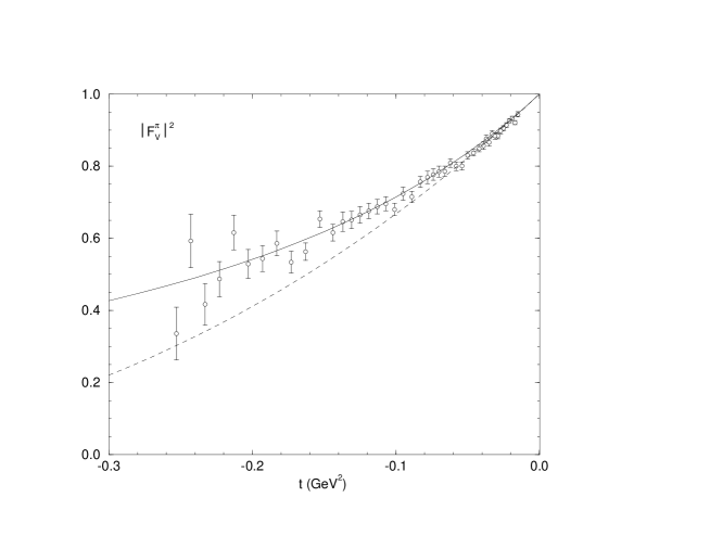
FIG. 1.: The pion vector form factor $|F_{V}^{\pi}|^{2}$ in the spacelike region. The solid line is the inverse-amplitude method, the dashed line one-loop ChPT, and the experimental data are from Ref. [10].

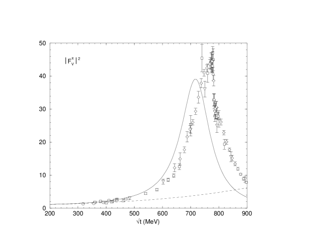
FIG. 2.: The pion vector form factor $|F_{V}^{\pi}|^{2}$ in the timelike region. The solid line is the inverse-amplitude method, the dashed line one-loop ChPT, and the experimental data are from Ref. [17] (circles), Refs. [14, 18] (squares), Ref. [19] (triangles), Ref. [20] (inverted triangles), and Ref. [21] (diamonds).

FIG. 3.: The real (a) and imaginary (b) part of the pion scalar form factor $F_{S}^{\pi}$. The solid line is the inverse-amplitude method, the dashed line one-loop ChPT, and the dashed-dotted line solution B from a dispersive analysis [7, 12].

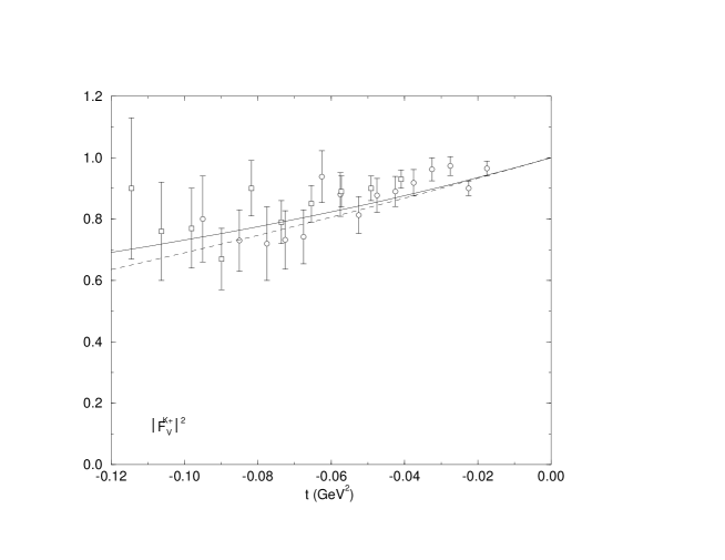
FIG. 4.: The charge kaon vector form factor $|F_{V}^{K^{+}}|^{2}$ in the spacelike region. The solid line is the inverse-amplitude method, the dashed line one-loop ChPT, and the experimental data are from Ref. [13] (circles) and Ref. [22] (squares).

FIG. 5.: The $K_{l3}$ form factors in the physical region. The numerical difference between the $K_{l3}^{+}$ and $K_{l3}^{0}$ form factors is negligible in this region. The solid line (inverse-amplitude method) and dashed line (one-loop ChPT) are for the $K_{l3}$ vector form factor $f_{+}^{K\pi}$, whereas the dash-dotted line (inverse-amplitude method) and dotted line (one-loop ChPT) are for the scalar form factor $f_{0}^{K\pi}$.