HD–THEP–96–47

hep-ph/9611250

Gluon-mass effects in quarkonia decays,
$e^{+}e^{-}$ annihilation and the scalar glueball current
Jue-ping Liu

Department of Physics, Wuhan University
Wuhan/Hubei 430072, P.R. of China

Werner Wetzel

Institut für Theoretische Physik, Universität Heidelberg
Philosophenweg 16, D-69120 Heidelberg,Germany

November 4, 1996

In this paper we continue previous efforts in the literature to determine phenomenological values for the gluon mass by confronting theoretical results obtained in a theory of massive gluons with experimental values or results directly referring to the nontrivial structure of the Yang-Mills vacuum, e.g. to the presence of the gluon condensate. The decays of heavy quarkonia into $3$ gluons and $2$ gluons + photon are considered in detail as well as the correlators of the electromagnetic current and the scalar glueball current. Based on the analysis for the latter quantities a value for the gluon mass in the range of 500-600 MeV is estimated from the standard SVZ-value of the gluon condensate.

1 Introduction

Starting with the original suggestion by Cornwall [1], the possibility of a nonzero gluon mass has been discussed in various contexts over the past 15 years. It has been argued (c.f. [2]) that the severe infrared singularities of the gluon interaction might resolve themselves in the creation of a gluon mass. The emergence of this mass might be closely related to the nontrivial nature of the QCD vacuum, in particular to the gluon condensate of Shifman, Vainshtein and Zakharov [3].

However unlike the by now very much established gluon condensate or the constituent mass of quarks, the concept of a gluon mass meets a lot of reservation as it touches the fundamental principles of gauge invariance and renormalizability.

As argued by many authors and in particular by [4], the only way to make massive nonabelian vector mesons compatible with a decent high energy behaviour, i.e. with renormalizability, seems to be the Higgs mechanism. The effective Lagrangian advocated in [2] for a massive gluon theory in fact can be understood as a Higgs model with the ramification that all physical Higgs particles have been removed from the theory by making them infinitely heavy. More precisely, this model is the generalization of the $SU(2)$ Higgs-model with a frozen radial degree of freedom to the case of the gauge group $SU(3)$. In this gauged nonlinear $\sigma$-model, the $8$ would-be Goldstone bosons provide the longitudinal polarization degrees of freedom for the gluons. In the unitary gauge, they are absorbed into the redefinition of the gauge field, leaving us with a massive vector boson theory with a global $SU(3)$ symmetry.

Though the conflict between a gluon mass and gauge invariance is avoided in this model, the renormalizability has obviously been lost in the way of going from a linear $\sigma$-model to the nonlinear one.

One of the main questions then is, how severe the loss of renormalizability really is. From the situation of $SU(2)$, where the resulting new divergence is only logarithmic in the cut-off or the physical Higgs mass - a fact known as screening theorem of Veltman [5] -, we may hope for a similar behaviour in the $SU(3)$ case. To clarify this point, the systematic analysis of [6] for the divergencies should be extended from $SU(2)$ to $SU(3)$.

Another critical issue to the significance of this model as an effective low energy theory is the confinement property. In the Higgs phase, i.e. the phase corresponding to superconductivity, magnetic monopoles are confined and the Wilson loop in the fundamental representation satisfies a perimeter law. It has been argued in [7] that at some critical coupling the model is expected to undergo a transition to a phase with condensed vortices. In this phase the ’t Hooft loop, i.e. the order parameter related to confinement of monopoles, can be shown to satisfy a perimeter law implying - according to the classification of phases by ’t Hooft [8] - an area law for the Wilson loop in the fundamental representation.

On the phenomenological side, effects of a finite gluon mass have been considered in the past for the standard quarkonium decays into gluons [9], potential models for glue-balls [10], approximations to the QCD-Hamiltonian combined with a variational method [11], a possible relation between the gluon condensate and the gluon mass through QCD sum-rules [12], the two-gluon exchange contribution to the Pomeron [13], and the vacuum functional of $SU(3)$ Yang-Mills theory [14].

In a recent analysis [15] of $J/\psi$ and $\Upsilon$ decays it was investigated in detail whether the deficiencies between experiment and theory for the total decay rate and the inclusive photon spectrum can be understood as being due to relativistic corrections or alternatively due to a finite gluon mass. The conclusion of [15] is that the relativistic corrections needed to bring experiment and theory into agreement do not scale in the expected manner when going from c-quarks to b-quarks. The alternative with a gluon mass leads to values of $.66GeV$ and $1.17GeV$ for $J/\psi$ and $\Upsilon$ decays, respectively. The authors interpret the rise of the gluon mass parameter as an indication that without phase-space limitation the true gluon mass would be of the order of $1.5GeV$ and is reduced to effectively smaller values due to phase space limitations in $\Upsilon$ and $J/\psi$ decays.

As a continuation of previous efforts to determine phenomenological values for the gluon mass, we treat in this paper the following three subjects. First we complete in section 2 the analysis of [15] by taking into account a finite gluon mass not only in the phase space but also in the amplitudes for $J/\psi$ and $\Upsilon$ decays. For this purpose we derive the analytical form of the Dalitz distributions for $(Q\bar{Q})_{1}^{3}\rightarrow 3g$, $(Q\bar{Q})_{1}^{3}\rightarrow\gamma+2g$ and $(Q\bar{Q})_{0}^{1}\rightarrow 2g$ for massive gluons to leading order in $\alpha_{s}$, thus extending the classical formulas originally derived for positronium decays (e.g. ref. [16]). Using these results we determine by a comparison with the results of [15] corrected values for the gluon mass.

As a further basic process affected by a finite gluon mass we consider in section 3 the $e^{+}e^{-}$ annihilation into mass-less quarks. The analytic form of the vacuum polarization to order $\alpha_{s}$ with a massive vector boson has been known for a long time [17]. Analyzing the dispersion relation for the derivative of the vacuum polarisation function, a systematic expansion in powers of $M^{2}/Q^{2}$ can be derived for the Euclidean region. This expansion can serve as a basis to relate the gluon mass M to the gluon condensate by equating the $1/Q^{4}$ term in this expansion with the $1/Q^{4}$ term in the operator product expansion as used before in ref. [12]. As it turns out, the expression obtained in this way is different from the expression in ref. [12], where a Mellin-transform technique has been used to isolate the $1/Q^{4}$ term in the loop diagrams. Our relation can be used to derive a simple expression for the gluon mass in terms of the gluon condensate.

In a similar spirit we deal in section 4 with the two-point function for the scalar glue-ball current instead of the electromagnetic current. Matching the result obtained for this two-point function in the massive theory with the result obtained from the operator expansion in the massless theory, a similar, albeit not exactly identical, relation between the gluon mass and the gluon condensate is obtained.

In section 5 finally the results are summarized and a few remarks concerning possible future directions of this research are made.

2 Heavy quarkonia decays into gluons

In this section we present our results for the decay rates of triplet $(Q\bar{Q})_{1}^{3}$ and singlet $(Q\bar{Q})_{0}^{1}$ $S$-wave quarkonia states into massive gluons. The calculation uses the standard approximation of neglecting the dependence on the momenta of the heavy quarks. Accordingly we can write:

$$d\Gamma((Q\bar{Q})\rightarrow..)\sim|\psi(0)|^{2}d\Gamma(Q+\bar{Q}\rightarrow..)$$ (1)

where $\psi(0)$ represents the spatial $Q\bar{Q}$ wave-function at the origin and $d\Gamma(Q+\bar{Q}\rightarrow..)$ is calculated with $Q$ and $\bar{Q}$ at rest.

We use $\eta=(M/2m)^{2}$ to parametrize the dependence on the ratio between gluon mass $M$ and quark mass $m$. On the level of our approximation, $2m$ of course can be identified with the mass of the respective singlet or triplet quarkonium state.

We start with the $S_{0}^{1}\rightarrow 2g$ decay rate which is given by:

$$\Gamma=\Gamma_{0}((1-4\eta)/(1-2\eta)^{2})(1-4\eta)^{1/2}$$ (2)

where $\Gamma_{0}$ is the decay rate for $M=0$ and the gluon mass effects on the amplitude squared and the phase space have been separated for convenience. As can be seen from eq.(2) the amplitude squared decreases with increasing $M$, though compared to the phase space the effect only starts at one order higher in $\eta$ .

For the Dalitz distribution of ${}^{3}S_{1}\rightarrow ggg$ we obtain the basic formula:

$$d\,\Gamma(^{3}S_{1}\rightarrow ggg)=$$

$$\,{{\Gamma_{0}}\over{\left(-9+{{\pi}^{2}}\right)}}\,{{\delta(-2\,\left(1-3\,\eta\right)+x_{1}+x_{2}+x_{3})\,dx_{1}\,dx_{2}\,dx_{3}}\over{{{x_{1}}^{2}}\,{{x_{2}}^{2}}\,{{x_{3}}^{2}}}}\,[$$

$$\eta\,{16\over 3}\,{{\left(1-3\,\eta\right)}^{2}}\,\left(1-{{51\,\eta}\over 8}-{{15\,{{\eta}^{2}}}\over 4}\right)$$

$$+\left({{x_{1}}^{2}}+{{x_{2}}^{2}}+{{x_{3}}^{2}}\right)\,\left(1-14\,\eta+48\,{{\eta}^{2}}+25\,{{\eta}^{3}}\right)$$

$$-2\,\left({{x_{1}}^{3}}+{{x_{2}}^{3}}+{{x_{3}}^{3}}\right)\,\left(1-{{17\,\eta}\over 3}-3\,{{\eta}^{2}}\right)$$

$$+\left({{x_{1}}^{4}}+{{x_{2}}^{4}}+{{x_{3}}^{4}}\right)\,\left(1+{{\eta}\over 2}\right)\,]$$

where the variables $x_{i}$ are related to the gluon energies $E_{i}$ by $x_{i}=E_{i}/m-2\eta$. Similar to before $\Gamma_{0}$ represents the integrated decay rate for mass-less gluons.

Apart from the constant term proportional to $\eta$ , eq.(2) has a similar form as in the mass-less case, i.e. the numerator of the distribution can be written as $(x_{1}^{2}P(x_{1})+cycl)$, where $P(x)$ is a second order polynomial in $x$. For $\eta=0$, $P$ reduces to the form $P(x)=(1-x)^{2}$, well known from the classic positronium formula.

When one of the gluons, say gluon 1, is replaced by a photon, the corresponding expression reads with $z=E_{\gamma}/m$ replacing $x_{1}$:

$$d\,\Gamma(^{3}S_{1}\rightarrow\gamma gg)=$$

$$\,{{\Gamma_{0}}\over{\left(-9+{{\pi}^{2}}\right)}}\,{{\delta(-2\,\left(1-2\,\eta\right)+z+x_{2}+x_{3})\,dz_{1}\,dx_{2}\,dx_{3}}\over{{{z}^{2}}\,{{x_{2}}^{2}}\,{{x_{3}}^{2}}}}\,[$$

$$+{8\over 3}\,\eta\,\left(1-{{25\,\eta}\over 2}\right)\,{{\left(1-2\,\eta\right)}^{2}}\,$$

$$+z\,32\,\left(1-2\,\eta\right)\,\left(1-{{\eta}\over 4}\right)\,{{\eta}^{2}}$$

$$+{{z}^{2}}\,\left(1-2\,\eta\right)\,\left(1-6\,\eta-6\,{{\eta}^{2}}\right)$$

$$-2\,{{z}^{3}}\,\left(1-{{10\,\eta}\over 3}-2\,{{\eta}^{2}}\right)$$

$$+{{z}^{4}}\,\left(1+{{\eta}\over 2}\right)$$

$$+\left({{x_{2}}^{2}}+{{x_{3}}^{2}}\right)\,\left(1-8\,\eta+22\,{{\eta}^{2}}+8\,{{\eta}^{3}}\right)$$

$$-2\,\left({{x_{2}}^{3}}+{{x_{3}}^{3}}\right)\,\left(1-{{10\,\eta}\over 3}-2\,{{\eta}^{2}}\right)$$

$$+\left({{x_{2}}^{4}}+{{x_{3}}^{4}}\right)\,\left(1+{{\eta}\over 2}\right)$$

$$-\left({{x_{2}}^{2}}\,{{x_{3}}^{2}}\right)\,\eta\,]$$

Using these expressions and integrating over phase space we can now make a simple analysis to estimate new values for the gluon mass which take into account both phase-space and amplitude effects. The results are shown in Figs. 1,2, where the integrated decay rate is plotted as a function of $M^{2}/4m^{2}$. As can be seen, the inclusion of the gluon mass in the amplitude leads to an increase of the decay rate. This feature might be expected on the basis that for massive gluons there are in addition the channels involving longitudinal gluons. Using the values for the gluon mass from ref.([15]) i.e. $M=.66GeV$ and $M=1.17GeV$ for $J/\psi$ and $\Upsilon$, respectively, we conclude that in order to reach the same level of suppression the gluon mass values change to $M=.76(.79)GeV$ and $M=1.41(1.4)GeV$, where the numbers in brackets refer to the case where the $\gamma+2g$ reaction is used to make the matching.

Figure 1: ${}^{3}S_{1}\rightarrow ggg$ decay rate as a function of $\eta=M^{2}/4m^{2}$, normalized to the decay rate for mass-less gluons. The dashed line represents the case when the gluon mass is only taken into account in the phase space. The dotted lines indicate how the gluon mass has to be changed to reach the same suppression when taking the gluon mass into account also in the amplitude

Figure 2: The analogue of Fig. 1 for ${}^{3}S_{1}\rightarrow\gamma+gg$

Another quantity of interest is the photon energy spectrum. The analytic form is given in the Appendix. Examples for the effect of the gluon mass on the shape of this distribution are shown in Fig. 3. As can be seen, the larger gluon mass needed to produce the same amount of suppression when the gluon mass effect is taken into account in both the amplitude and the phase space, leads to a sharper cut-off at the end of the spectrum. However, in this region we cannot take the massive gluon model really serious, and there are other effects like the Fermi-motion of the quarks to which this behaviour is sensitive to.

Figure 3: The normalized photon energy spectrum for $\Upsilon\rightarrow\gamma+gg$ as a function of $z=E_{\gamma}/m$. The pair of gluon mass values chosen, i.e. $M=1.41GeV$ and $M=1.17GeV$, are the ones determined above to reproduce the experimental suppression of the total decay rate. As before, the dashed line is the curve involving the phase-space effect only. For comparison also the spectrum for zero gluon mass is shown (dotted line)

3 $e^{+}e^{-}$ annihilation

Figure 4: The leading order diagrams with a gluon of mass $M$

As a further basic process we consider now the leading order effect of a massive gluon on the electro-magnetic vacuum polarisation, i.e. the diagrams given in Fig. 4. To simplify matters, we take the massless quark limit. A systematic expansion in terms of $M^{2}/Q^{2}$ can most easily be derived starting from the dispersion relation for the derivative of the vacuum polarisation function.

$${\rm D}({Q^{2}})={Q^{2}}\,\left(\int_{0}^{\infty}ds\,{{R(s)}\over{{{\left({Q^{2}}+s\right)}^{2}}}}\right)$$ (5)

The imaginary part $R$ for the diagrams in Fig. 4 has been known for a long time [17], and for $x=M^{2}/s<1$ is given by:

$$R(x)=$$

$${{N_{c}^{2}-1}\over{4\,N_{c}}}\,({3\over 2}-2\,x-5\,{x^{2}}+2\,x\,\ln(x)+3\,{x^{2}}\,\ln(x)$$

$$\hskip 73.97733pt-2\,{{\left(1+x\right)}^{2}}\,\left(\ln(x)\,\ln(1+x)+Li_{2}(-x)\right)\,)$$

For convenience the normalisation has been factored out, i.e. $N_{c}\,\alpha_{s}/\pi$ for a single quark flavor with unit charge and $N_{c}$ colours. Eq.(3) also determines $R$ for $x>1$ through the symmetry relation:

$$R(x)=\left(1-{x^{2}}\right)\,R(0)+{x^{2}}\,R({1\over x})$$ (7)

The function $R(x)$ has the small-$x$ expansion:

$$R(x)\,/\,({{N_{c}^{2}-1}\over{N_{c}}})\,{3\over 8}=\hat{R}(x)=1+\left(\sum_{k=2}^{\infty}a_{k}\,{x^{k}}\right)+\left(\sum_{k=3}^{\infty}b_{k}\,{x^{k}}\,\ln(x)\right)$$ (8)

As a consequence, the following expansion for $D(Q^{2})$ in terms of $M^{2}/Q^{2}$ can be derived:

$$D(Q^{2})\,/\,({{N_{c}^{2}-1}\over{N_{c}}})\,{3\over 8}=$$ (10)

$$1+{{{M^{2}}}\over{{Q^{2}}}}\,2\,\left(\int_{0}^{1}dx\,{{\hat{R}(x)-1}\over{{x^{2}}}}\right)$$

$$+{\left(\,{{M^{2}}\over{Q^{2}}}\,\right)}^{2}\,\left(a_{2}\,(2\,\ln({{{M^{2}}}\over{{Q^{2}}}})+1)-2\int_{0}^{1}dx\,{{\hat{R}(x)-1}\over x}-2\int_{0}^{1}dx\,{{\hat{R}(x)-1-a_{2}\,{x^{2}}}\over{{x^{3}}}}\right)$$

$$+{{{\rm O}({{{M^{2}}}\over{{Q^{2}}}})}^{3}}$$

Numerically we have:

$$a_{2}=-1$$

$$\int_{0}^{1}dx\,{{\hat{R}(x)-1}\over x}=-7+{{4\,{{\pi}^{2}}}\over 9}+2\,{\rm\zeta}(3)=-0.209$$

$$\int_{0}^{1}dx\,{{\hat{R}(x)-1}\over{{x^{2}}}}={{-16}\over 3}+4\,{\rm\zeta}(3)=-0.525$$

$$\int_{0}^{1}dx\,{{\hat{R}(x)-1+{x^{2}}}\over{{x^{3}}}}={{57-8\,{{\pi}^{2}}+36\,{\rm\zeta}(3)}\over{18}}=1.184$$

Equation (10) should be compared with the result from the operator-product expansion:

$$D(Q^{2})={{N_{c}^{2}-1}\over{N_{c}}}\,{3\over 8}+{{\pi}\over{\alpha_{s}}}\,{{{2\,\pi}^{2}}\over N_{c}}\,<{{\alpha_{s}\over{\pi}}\,GG}>{1\over{Q^{4}}}+O({{1}\over{Q^{6}}})$$ (12)

The first term represents the perturbative contribution from the diagrams in Fig.4 with massless gluons, and the second term is the contribution from the gluon condensate as given in ref. [3] (in our normalization). Equating the $1/Q^{4}$ terms in (10) and (12), we obtain:

$$<{{\alpha_{s}\over{\pi}}\,GG}>={{\alpha_{s}}\over{\pi}}\,{{3(N_{c}^{2}-1)}\over{16\,{{\pi}^{2}}}}\,{M^{4}}\,\left({{20}\over 3}-8\,\zeta(3)-2\,\ln({{{M^{2}}}\over{{Q^{2}}}})\right)$$ (13)

The corresponding expression derived in [12] reads:

$$<{{\alpha_{s}\over{\pi}}\,GG}>={{\alpha_{s}\over{\pi}}\,{{3(N_{c}^{2}-1)}\over{16\,\pi}^{2}}}\,{M^{4}}\,\left({{45}\over 8}+{{10}\over 3}\,\zeta(3)-{{5\,{{\pi}^{2}}}\over{27}}-{5\over{18}}\,\ln({{{M^{2}}}\over{{Q^{2}}}})-{5\over 9}\,{{\ln({{{M^{2}}}\over{{Q^{2}}}})}^{2}}\right)$$ (14)

which has no resemblance to what we have obtained.

At present the origin of this discrepancy is not satisfactorily explained. However, since our own calculation only uses standard Feynman diagram techniques and has been checked by an independent calculation where the diagrams in Fig.4 are calculated by a numerical procedure along the lines of ref. [18], we suspect that the Mellin transform technique used in ref. [12] has not been properly applied.

A $Q^{2}$-independent relation between M and the gluon condensate can be obtained from eq.(13) by using for $\alpha_{s}/\pi$ the standard expression $4/\beta_{0}ln(Q^{2}/\Lambda^{2})$ for the running coupling with $\beta_{0}=N_{c}11/3$ and evaluating eq.(13) to leading order in $ln(Q^{2})$. The result is:

$$M^{4}={{22}\over{9}}\,\pi^{2}\,{{N_{c}}\over{(N_{c}^{2}-1)}}\,<{{\alpha_{s}}\over{\pi}}\,GG>$$ (15)

yielding $M\simeq 570MeV$ for $N_{c}=3$ and the standard SVZ-value for the gluon condensate $<{{\alpha_{s}\over{\pi}}\,GG}>=(.33GeV)^{4}$.

4 Scalar glue-ball current

Instead of the electromagnetic current we consider in this section the scalar glue-ball current defined in terms of the gluon field-strength tensor $G^{a}_{\mu\nu}$ by

$$\hat{j}=G^{a}_{\mu\nu}G^{a\mu\nu}$$ (16)

For ease of writing we use $\hat{j}$ to denote the current with a unit normalization factor and $j$ for the current with a normalization factor $\alpha_{s}/\pi$ which turns $j$ into a renormalization group invariant quantity .

As a first step we calculate the diagram in Fig. 5 for $\hat{j}$ in the massive theory. Defining $\hat{\pi}_{GG}(Q^{2})$ for euclidean $q^{2}=-Q^{2}$ by:

$$<\hat{j}\,\hat{j}>=i\,{{N_{c}^{2}-1}\over{2\pi^{2}}}\,\hat{\pi}_{GG}(Q^{2})$$ (17)

we obtain:

$$\hat{\pi}_{GG}(Q^{2})\cong\left({1\over 2}\,{{\left({Q^{2}}+2\,{M^{2}}\right)}^{2}}+{M^{4}}\right)\,\left(\int_{0}^{1}d\alpha\,\ln(1+{{\alpha\,\left(1-\alpha\right)\,{Q^{2}}}\over{{M^{2}}}})\right)$$ (18)

where $\cong$ means equality up to polynomial terms which do not survive a three-fold subtraction needed to remove the UV-divergencies. From (18) we obtain the following expansion in terms of $M^{2}/Q^{2}$:

$$Q^{2}\,({{d}\over{dQ^{2}}})^{3}\,\hat{\pi}_{GG}=1-3\,{{M^{2}}\over{Q^{2}}}+12\,({{M^{2}}\over{Q^{2}}})^{2}+{\rm O}({{M^{2}}\over{Q^{2}}})^{3}$$ (19)

which is free of logarithmic factors $ln(M^{2}/Q^{2})$ up to order $1/Q^{4}$. As visible from this expression, the normalization of $\hat{\pi}_{GG}$ has been chosen such that the third derivative equals to one in the massless limit.

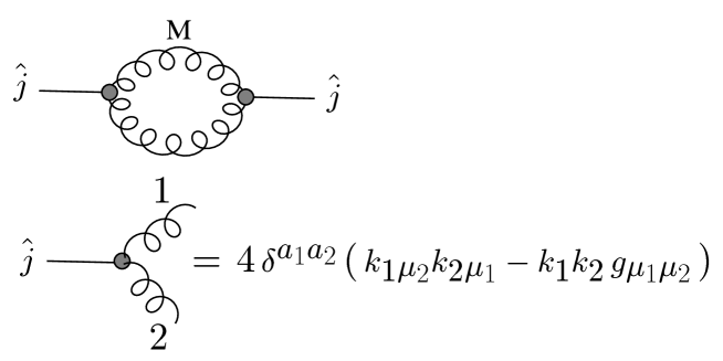
Figure 5: The leading order diagram for the scalar glueball current with a gluon of mass $M$, and the expression for the vertex.

As a second step we make a renormalization-group analysis for the coefficient function of the gluon condensate $<j>$ in the operator- product expansion of the two-point function $\pi_{GG}$ for the scalar current $j=(\alpha_{s}/\pi)\,\hat{j}$:

$$\pi_{GG}={\rm C}_{pert}(Q^{2})\,1+{\rm C}_{GG}(Q^{2})\,<j>+\,...$$ (20)

The coefficient function $C_{GG}$ has the following expansion in $\alpha_{s}/\pi$ :

$$C_{GG}(Q^{2})={{\alpha_{s}({{\mu}^{2}})}\over{\pi}}\,{\rm C}_{0}+({{{\alpha_{s}({{\mu}^{2}})}\over{\pi}}})^{2}\,{\rm C}_{1}({{{{\mu}^{2}}}\over{{Q^{2}}}})+\,...$$ (21)

where $C_{0}$ is a constant whose value can be found from applying Wick’s theorem to the product of currents $j(x)j(0)$:

$$C_{0}=-\,{{8\pi^{2}}\over{N_{c}^{2}-1}}$$ (22)

Independence of $C_{GG}$ from the renormalization point $\mu$ requires the coefficient $C_{i}$ in (21) to be a polynomial of degree $i$ in the variable $ln(\mu^{2}/Q^{2})$. Choosing $\mu^{2}=Q^{2}$ and using the $1$-loop expression for $\alpha_{s}(Q^{2})/\pi$, we obtain:

$$Q^{2}\,({{d}\over{dQ^{2}}})^{3}\,C_{GG}(Q^{2})={{1}\over{(Q^{2})^{2}}}\,(-8\,{{C_{0}}\over{\beta_{0}\,ln(Q^{2}/\Lambda^{2})^{2}}}+O(ln(Q^{2}/\Lambda^{2})^{-3})\,\,)$$ (23)

where $\beta_{0}\,=\,11/3\,N_{c}$

The desired relation between M and the gluon condensate is now obtained by matching the $1/Q^{4}$ terms in eq.(23) and $(\alpha_{s}(Q^{2})/\pi)^{2}\,\times\,eq.(\ref{GG-pihat:3})$. The result is:

$$M^{4}={{11}\over{9}}\,\pi^{2}\,{{N_{c}}\over{N_{c}^{2}-1}}\,<{{\alpha_{s}\over{\pi}}\,GG}>$$ (24)

Comparing with the result obtained in section 3 in eq.(15), we recognize that we have almost obtained the same result except that the numerical coefficient is smaller by a factor of $2$. Thus the previous estimate for $M$ is reduced from $570MeV$ to $M\simeq 480MeV$

It is interesting to compare eq.(24) with the result of ref.([14]) obtained by a variational investigation of an ansatz for the vacuum functional. Again both results have the same structure and color dependence (large $N_{c}$). However, here there is a large difference in the numerical constant, i.e. $120$ for ref.([14]) instead of $11/9$. As a consequence their mass estimate is larger by a factor $\simeq 3$.

5 Summary and Outlook

In this paper we have continued previous attempts to estimate values for the gluon mass by confronting results obtained in leading order calculations for massive gluons with experimental results; either by a direct comparison as for $J/\psi$ and $\Upsilon$ decays or in a more indirect way by matching against nonperturbative contributions in the correlator of the electromagnetic current or the scalar glue-ball current. For the decays of heavy quarkonia the Dalitz distributions involving $2-$ or $3-$ massive gluons were derived, extending thus the basic formulae originally derived for positronium to this more general case. We then analyzed the leading QCD correction of the electromagnetic vacuum polarisation and determined the coefficients in an expansion in $1/Q^{2}$ which are relevant for a comparison with the leading nonperturbative contribution for this quantity. We found a different result for the $1/Q^{4}$-coefficient as previously given in the literature and claim that our result is correct as it has been checked by a completely different method than the one presented in this paper. Our result was then used to derive a simple renormalization-group invariant expression between the gluon mass and the gluon condensate. Finally a similar kind of analysis was applied to the correlator of the scalar glue-ball current where gluon mass effects already appear on the $1$-loop level. Again this leads to a relation between the gluon mass and the gluon condensate which is renormalization group invariant although with a slightly different numerical coefficient.

Taken at face value, there is a large spread between the mass estimates from heavy quarkonia decays, in particular the $\Upsilon$-decays where we can expect gluon mass effects to have fully developed, and the values obtained from the analysis of the correlators. Certainly the value of $M\simeq 1.4GeV$ obtained from $\Upsilon$-decays should be considered as an upper bound, since the starting values of [15] for the gluon mass have been obtained under the assumption that the main suppression comes from the gluon mass, not the relativistic corrections. As argued for instance in [19], the pattern of suppressions in the total $J/\psi$ and $\Upsilon$ decay rates can quantitatively be reproduced if the momentum dependence of the quarks is taken into account. Whether this straightforward incorporation of relativistic effects is legitimate is, however, still under debate (see [15]), and therefore a substantial gluon mass - though smaller in magnitude than the values discussed here - may indeed be required by the data. The results from matching the leading nonperturbative correction in the correlator for the electromagnetic and the scalar glueball current are equal to each other up to a factor of $2$ in the relation for $M^{4}$. Although this has little effect on the numerical value of the gluon mass $M$, the dependence on the process remains to be explained. In this context it would also be interesting to derive the expansion in powers of $M/M_{Q\bar{Q}}$ of the total decay rates of heavy quarkonia discussed in section 2 and match them likewise against the leading nonperturbative correction from the gluon condensate.

A more complete analysis should also cover the $1/Q^{2}$ corrections obtained in the massive theory, which seem to have no correspondence in the operator-product expansion. It has been argued in ref.([12]) that these corrections cancel against corrections from the formation of a vortex condensate. We believe that this proposition requires further examination.

6 Acknowledgement

One of us (W.W.) would like to thank the Physics Department of Wuhan University for the kind hospitality which has been extended to him in 1995 and 1996 on the occasion of his visits as foreign scholar.

7 Appendix

For the distribution of the photon in ${}^{3}S_{1}\rightarrow\gamma+gg$ the following expression is obtained from eq.(2) by integrating over the gluons.

$${{d\,\Gamma}\over{dz}}\propto$$

$${{x_{+}-x_{-}}\over{{z^{2}}}}$$

$$+\,{{ln(x_{+}/x_{-})}\over{{z^{2}}\,{{\left(-2+4\,\eta+z\right)}^{3}}}}\,[8\,{{\left(-1+2\,\eta\right)}^{2}}\,\left(2-4\,\eta+7\,{{\eta}^{2}}\right)$$

$$+8\,\left(-1+2\,\eta\right)\,\left(5-12\,\eta+10\,{{\eta}^{2}}+2\,{{\eta}^{3}}\right)\,z$$

$$+2\,\left(-1+2\,\eta\right)\,\left(-17+10\,\eta+6\,{{\eta}^{2}}\right)\,{z^{2}}$$

$$+2\,\left(-5+2\,\eta+2\,{{\eta}^{2}}\right)\,{z^{3}}\,]$$

$$+\,{{(1/x_{-}-1/x_{+})}\over{{z^{2}}\,{{\left(-2+4\,\eta+z\right)}^{2}}}}\,[4\,{{\left(-1+2\,\eta\right)}^{2}}\,\left(1+3\,{{\eta}^{2}}\right)$$

$$+4\,\left(-1+2\,\eta\right)\,\left(3-4\,\eta+2\,{{\eta}^{2}}+2\,{{\eta}^{3}}\right)\,z$$

$$+2\,\left(7-18\,\eta+10\,{{\eta}^{2}}+10\,{{\eta}^{3}}\right)\,{z^{2}}$$

$$+4\,\left(2+\eta\right)\,\left(-1+2\,\eta\right)\,{z^{3}}+\left(2+\eta\right)\,{z^{4}}\,]$$

Here $z=E_{\gamma}/m$ in terms of the photon energy $E_{\gamma}$, and

$$x_{\pm}=1-2\,\eta-{z\over 2}\pm{z\over 2}\,{\sqrt{1-{{4\,\eta}\over{1-z}}}}$$ (26)

delineate the boundary of the Dalitz plot in the plane $(x_{2},z)$ with $x_{2}=E_{2}/m-2\eta$.

References

- [1] J.M. Cornwall, Nucl. Phys B157 (1979) 392
- [2] J.M. Cornwall, Phys.Rev D26 (1982) 1453
- [3] M.A. Shifman, A.I. Vainshtein, V.I Zakharov, Nucl.Phys. B147 (1979) 385
- [4] C.H. Llewellyn Smith, Phys.Lett 46B (1973) 233, J.M. Cornwall et al, Phys.Rev.Lett 30 (1973) 1268
- [5] M. Veltman, Acta Physica Polonia, B12 (1981) 437
- [6] T. Appelquist, C. Bernard, Phys.Rev D22 (1980) 200
- [7] R. Akhoury, Nucl.Phys. B234 (1984) 533
- [8] G. t’Hooft, Nucl.Phys B138 (1978) 1, ibid B153 (1979) 141
- [9] G. Parisi, R. Petronzio, Phys. Lett 94B (1980) 51
- [10] J.M. Cornwall, A. Soni, Phys. Lett 120B (1983) 431
- [11] A. Szczepaniak, E.S. Swanson, C.-R. Ji, S.R. Cotanch, Phys. Rev. Lett.76 (1996) 2011 (hep-ph/9511422)
- [12] F.R. Graziani, Z.Phys. C33 (1987) 397
- [13] F. Halzen, G. Krein, A.A. Natale, Phys.Rev D47 (1993) 295
- [14] I.I. Kogan, A. Kovner, Phys. Rev. D52 (1995) 3719, (hep-th/9408081)
- [15] M. Consoli, J.H. Field, Univ. Geneva preprint UGVA-DPNC 1994/12-164
- [16] Landau-Lifschitz, Quantum Electrodynamics
- [17] W. Wetzel, W. Bernreuther, Phys.Rev. D24 (1981) 2724
- [18] P. Cvitanovic, T. Kinoshita, Phys.Rev. D10 (1974) 3978, 3991
- [19] H.C. Chiang, , J. Hüfner, H.J. Pirner, Phys. Lett 324B (1994) 482