SU(3) Breaking in Neutral Current Axial Matrix Elements
and the Spin-Content of the Nucleon

Abstract

We examine the effects of SU(3) breaking in the matrix elements of the flavour-diagonal axial currents between octet baryon states. Our calculations of $K,\eta$ and $\pi$ loops indicate that the SU(3) breaking may be substantial for some matrix elements and at the very least indicate large uncertainties. In particular, the strange axial matrix element in the proton determined from the measurements of $g_{1}(x)$ is found to have large uncertainties and might yet be zero. We estimate the strange axial matrix element in the proton to be $-0.35\ \raisebox{-3.01385pt}{$\stackrel{{\scriptstyle\textstyle<}}{{\sim}}$ }\ \Delta s\ \raisebox{-3.01385pt}{$\stackrel{{\scriptstyle\textstyle<}}{{\sim}}$ }\ 0$ and the matrix element of the flavour-singlet current in the proton to be $-0.1\ \raisebox{-3.01385pt}{$\stackrel{{\scriptstyle\textstyle<}}{{\sim}}$ }\ \Sigma\ \raisebox{-3.01385pt}{$\stackrel{{\scriptstyle\textstyle<}}{{\sim}}$ }\ +0.3$ from the E-143 measurement of $\int dx\ g_{1}(x)\ =\ 0.127\pm 0.004\pm 0.010$ .

The up-quark content of the $\Xi^{-}$ is discussed and its implications for nonleptonic weak processes discussed. We also estimate the matrix element of the axial current coupling to the $Z^{0}$ between all octet baryon states. This may be important for neutrino interactions in dense nuclear environments, where hyperons may play an important role.

October 1996

One of the more exciting realizations in hadronic physics of the last few years is that the strange quark may play an important role in the structure of the nucleon [1] . While this may seem somewhat unnatural in the context of the most naive quark model, it is perfectly natural from the standpoint of QCD. Matrix elements of the strange-vector current must vanish at zero-momentum transfer between states with zero net-strangeness, however, matrix elements of the axial current need not. Recent measurements suggest that the matrix element of the strange axial current in the proton is $\Delta s=-0.12\pm 0.04$ [2] . In addition, one would like to know what fraction of the nucleon spin is carried by the quarks themselves, which is equivalent to determining the matrix element of flavour singlet axial current in the proton, $\Sigma$ . This is, of course, intimately related to the matrix element of the strange axial current and present analysis suggests that $\Sigma=0.2\pm 0.1$ [2] , much smaller than the quark model estimate of $\Sigma\sim 0.58$. There have been intense theoretical and experimental efforts to extract $\Delta s$ and $\Sigma$ to address the present “spin-crisis” and such efforts continue (for recent reviews, see [3, 4]) .

A vital ingredient in the present determination of $\Sigma$ and $\Delta s$ is the matrix element of the $j_{5}^{\mu,8}=\overline{u}\gamma^{\mu}\gamma_{5}u+\overline{d}\gamma^{\mu}\gamma_{5}d-2\overline{s}\gamma^{\mu}\gamma_{5}s$ axial current in the nucleon, which cannot be measured directly but must be inferred from the approximate SU(3) symmetry observed in nature. The question of SU(3) breaking in the matrix element of the $j_{5}^{\mu,8}$ current has been previously addressed [5, 6, 7]. In [6]  it was assumed that the breaking in the matrix elements of the axial currents was proportional to the breaking in the octet baryon masses and in [5] a model of the SU(3) breaking was employed. A more systematic approach was that of [7] in which the breaking was analyzed in the context of the large-$N_{C}$ limit of QCD. It was found that the matrix element of the $j_{5}^{\mu,8}$ axial current was substantially reduced from its value in the symmetry limit.

In the limit of flavour SU(3) symmetry the three light quark contributions to the nucleon axial matrix elements are uniquely determined by three low energy observables. In this limit, two of these observables, $F$ and $D$, can be extracted from nuclear $\beta$-decay and from the semileptonic decay of strange hyperons. The third experimental constraint comes from a measurement of the axial singlet current in the nucleon, presently accomplished by measuring the $g_{1}(x)$ spin dependent structure function of the nucleon [9, 10] and using the SU(3) symmetry to remove the flavour octet contributions. In the real world we know that this symmetry is only approximate, broken by the difference between the mass of the strange quark and of the up and down quarks. Each of the matrix elements of the octet and singlet axial currents will receive SU(3) breaking contributions, with the leading contributions having the form $m_{s}\log m_{s}$ followed by terms of the form $m_{s}$ and higher. The leading contributions with non-analytic dependence on $m_{s}$ arise from hadronic kaon loops while terms analytic in the strange quark mass do not uniquely arise from such loops and must be fixed by other observables.

In this work we include all terms of the form $m_{s}\log m_{s}$ to the axial matrix elements appearing in hyperon decay and $\beta$-decay used to determine the axial couplings $F,D,C$ and $H$. We use these fits to predict matrix elements relevant for determining $\Sigma$ , $\Delta s$ and for the interaction of neutrinos with hyperons, a situation that may be important at high matter densities [11, 12] . Unfortunately, higher order SU(3) breaking contributions can only be estimated to be of order $M_{K}^{2}/\Lambda_{\chi}^{2}\sim 0.25$ (which is not to be confused with a $25\%$ correction to each matrix element). Part of the terms at this order (in fact a summation to all orders) arise from graphs involving the decuplet of baryon resonances as intermediate states. Such contributions are also present in the flavour-diagonal axial matrix elements with the same uncertainty arising from omission of incalculable terms ${\cal O}(m_{s})$ and higher. It is clear that our work provides merely an estimate for the size of SU(3) breaking in these matrix elements, however, the terms considered here are formally dominant in the chiral limit.

It is conventional to define the axial matrix elements of the quarks in the proton, $|P\rangle$, via

$$2s_{\mu}\ \Delta q = \langle P|\ \overline{q}\gamma_{\mu}\gamma_{5}q\ |P\rangle\ \ \ ,$$ (1)

where $q=u,d,s$ denotes the quark flavour, and $s_{\mu}$ is the nucleon spin vector. Any linear combination of the three light quark neutral axial currents can be written in terms of the two diagonal octet generators and the singlet. In deep-inelastic scattering one measures the matrix element of the current

$$j_{5}^{\mu} = \overline{q}\ {\cal Q}^{2}\ \gamma^{\mu}\gamma_{5}\ q\ \ \ ,$$ (2)

in the proton, where ${\cal Q}$ is the light quark charge matrix, given by

$${\cal Q} = {1\over 3}\left(\matrix{2&0&0\cr 0&-1&0\cr 0&0&-1}\right)\ \ \ .$$ (3)

In conjunction with a measurement of the matrix elements of the flavour diagonal currents

$$j_{5}^{\mu,3} = \ \overline{q}\ {\cal O}_{3}\gamma_{\mu}\gamma_{5}\ q\ \ \ \ ,\ \ \ \ j_{5}^{\mu,8}=\ \overline{q}\ {\cal O}_{8}\gamma_{\mu}\gamma_{5}\ q\ \ \ \ ,$$ (4)

in the proton, where we use

$${\cal O}_{3} = \left(\matrix{1&0&0\cr 0&-1&0\cr 0&0&0}\right)\ \ \ \ ,\ \ \ \ {\cal O}_{8}=\left(\matrix{1&0&0\cr 0&1&0\cr 0&0&-2}\right)\ \ \ \ ,$$ (5)

the flavour singlet or alternately the strange quark contribution may be extracted via

$$\left(\matrix{1&0&0\cr 0&1&0\cr 0&0&1}\right) = {9\over 2}{\cal Q}^{2}-{3\over 4}{\cal O}_{3}-{1\over 4}{\cal O}_{8}$$ (6)

$$\left(\matrix{0&0&0\cr 0&0&0\cr 0&0&1}\right) = {3\over 2}{\cal Q}^{2}-{1\over 4}{\cal O}_{3}-{5\over 12}{\cal O}_{8}\ \ \ \ .$$ (7)

The matrix element of $j_{5}^{\mu,3}$ in the nucleon is well determined from nuclear $\beta$-decay via isospin symmetry, leading to

$$\Delta u\ -\ \Delta d = g_{A}\ =\ 1.2664\pm 0.0065\ \ \ ,$$ (8)

where we have neglected isospin breaking effects. Unfortunately, we cannot use isospin to relate the matrix element of $j_{5}^{\mu,8}$ in the proton to any other set of physical observables We must resort to using flavour SU(3) symmetry as a starting point and systematically determine corrections arising from SU(3) breaking.

Let us begin by discussing the matrix element of the axial currents in the limit of exact SU(3). The matrix elements between baryons in the lowest lying octet of the axial currents transforming as octets under SU(3) are described by the following effective lagrange density

$$j_{5,{\rm eff.}}^{\mu,a} = D\ Tr\left[\overline{B}\ 2s_{\mu}\{{\cal O}_{a},B\}\right]\ +\ F\ Tr\left[\overline{B}\ 2s_{\mu}[{\cal O}_{a},B]\right]\ \ \ ,$$ (9)

where $B$ is the octet of baryon fields

$$B=\left(\matrix{\Lambda/\sqrt{6}+\Sigma^{0}/\sqrt{2}&\Sigma^{+}&p\cr\Sigma^{-}&\Lambda/\sqrt{6}-\Sigma^{0}/\sqrt{2}&n\cr\Xi^{-}&\Xi^{0}&-2\Lambda/\sqrt{6}}\right)\ \ \ \ .$$ (10)

Also, the matrix element of the singlet current is reproduced by the lagrange density

$$j_{5,{\rm eff.}}^{\mu,1} = STr\left[\overline{B}\ 2s_{\mu}\ B\right]\ \ \ .$$ (11)

At tree-level we can determine the parameters $F$ and $D$ by fitting the theoretical expression, linear in $F$ and $D$, to the observed rates for $n\rightarrow pe^{-}\overline{\nu}_{e}$, $\Sigma^{-}\rightarrow ne^{-}\overline{\nu}_{e}$, $\Xi^{-}\rightarrow\Lambda e^{-}\overline{\nu}_{e}$, $\Sigma^{-}\rightarrow\Lambda e^{-}\overline{\nu}_{e}$, $\Xi^{-}\rightarrow\Sigma^{0}e^{-}\overline{\nu}_{e}$ and $\Lambda\rightarrow pe^{-}\overline{\nu}_{e}$. However, one must keep in mind that we expect deviations between the “best fit” and the experimental results to be at the $\sim 25\%$ level due to the fact that the theoretical expressions have been truncated, and terms of order ${\cal O}\left(m_{s},\ m_{s}\log m_{s},...\right)$ have been neglected [8] . This includes the fit to the experimentally well measured value of $g_{A}$, equal to $D+F$ in the SU(3) limit (i.e. we naively expect to see $D+F$ deviate from $g_{A}$ at the $25\%$ level in the best fit). In the matrix elements we use to fit the axial couplings the experimental uncertainties are much less than the corresponding theoretical uncertainty. To determine $F$ and $D$ we minimize a $\chi^{2}$ function

$$\chi^{2} = \sum_{\rm data}\ {({\rm expt}_{i}-{\rm theory}_{i})^{2}\over\sigma_{\rm theory}^{2}}\ \ \ ,$$ (12)

where ${\rm expt}_{i}$ denotes an experimental measurement of an axial matrix element, ${\rm theory}_{i}$ denotes its theoretical value for given values of $F$ and $D$, and $\sigma_{\rm theory}$ denotes the theoretical uncertainty which we somewhat arbitrarily choose to be $\sim 0.2$, and equal for all data points, i.e. an unweighted fit. This is in contrast to the fit made by Jaffe and Manohar in [8] and is a more extreme version of a fit made in [7] . The uncertainties we quote for the couplings $F$ and $D$ are found by requiring that $\chi^{2}<\chi^{2}_{\rm min.}+2.3$, corresponding to a $68\%$ confidence interval. It is clear that this analysis can only provide an estimate of the uncertainties as the pattern of breaking will not be uncorrelated for these processes. We find that

$$D = 0.79\pm 0.10$$ (13)

$$F = 0.47\pm 0.07\ \ \ .$$ (14)

The errors on $D$ and $F$ are highly correlated and one finds that the “best fit” value for $D+F$ is $1.26\pm 0.08$. Further, the best for $3F-D$ (the tree-level expression for the matrix element of the ${\cal O}_{8}$ current) is $0.65\pm 0.21$, in agreement with the central value of $0.60$ found in [8]. The values of $F$ and $D$ are in agreement with those found in [7] except the uncertainties found from our somewhat ad hoc procedure are larger, but they do represent a reasonable estimate of the true uncertainties.

A third input required to fix the individual quark axial matrix elements in the proton is measured in deep-inelastic scattering

$$2s_{\mu}\int_{0}^{1}\ dx\ g_{1}(x,Q^{2}) = \ {1\over 2}\left(1-{\alpha_{s}(Q^{2})\over\pi}\right)\langle P|\overline{q}\ {\cal Q}^{2}\ \gamma_{\mu}\gamma_{5}\ q|P\rangle$$ (15)

$$= \ {1\over 9}\left(1-{\alpha_{s}(Q^{2})\over\pi}\right)\langle P|{3\over 4}\overline{q}\ {\cal O}_{3}\ \gamma_{\mu}\gamma_{5}\ q\ +\ {1\over 4}\overline{q}\ {\cal O}_{8}\ \gamma_{\mu}\gamma_{5}\ q\ +\ \overline{q}\ I\ \gamma_{\mu}\gamma_{5}\ q|P\rangle\ \ \ \ ,$$ (16)

where $I$ is the identity matrix. The two recent measurements of this quantity are

$$\int_{0}^{1}\ dx\ g_{1}(x,Q^{2}=3{\rm GeV}^{2}) = 0.127\pm 0.004\pm 0.010\ \ \ ,$$ (17)

by the E-143 collaboration [10] and

$$\int_{0}^{1}\ dx\ g_{1}(x,Q^{2}=10{\rm GeV}^{2}) = 0.136\pm 0.011\pm 0.011\ \ \ ,$$ (18)

by the SMC collaboration [9]. We choose to use the E-143 measurement at $Q^{2}=3{\rm GeV}^{2}$ for our evaluations and find at tree-level

$$\Delta u\ +\ \Delta d\ +\ \Delta s = 0.10\pm 0.10\ =\ \Sigma\ \ \ \ ,$$ (19)

which along with the octet matrix elements allows us to separate the quark contributions

$$\Delta u = 0.77\pm 0.04\ \ ,\ \ \Delta d\ =\ -0.49\pm 0.04\ \ ,\ \ \Delta s\ =\ -0.18\pm 0.09\ \ \ \ .$$ (20)

These values are consistent with the analysis of Jaffe and Manohar in [8]. The $Q^{2}$ dependence of $\Sigma$ is very weak [13, 14] (see also [8] and [15]) and so we set $\Sigma\sim S$.

We can estimate the leading SU(3) breaking to each axial matrix element in chiral perturbation theory. It is of the form $m_{s}\log m_{s}$ arising from the infrared region of hadronic loops involving $K$’s, $\eta$’s and $\pi$’s and can be computed exactly. Such loop graphs are divergent and require the presence of a local counterterm analytic in the light quark masses which must be fit to data. Some effects of $K$ and $\eta$ loops on strange quark observables in the nucleon have been considered previously, e.g. [16, 17] .

For some hyperon decays the axial matrix element is determined from an experimental measurement of the ratio of vector to axial vector matrix elements. The Ademollo-Gatto theorem [18] protects the vector matrix elements from corrections of the form $m_{s}\log m_{s}$, with leading corrections starting at ${\cal O}(m_{s})$ [19] . Consequently, at the order to which we are working we can consistently ignore deviations of the vector matrix elements due to SU(3) breaking and extract the axial matrix elements from the ratio of axial to vector current matrix elements.

Heavy baryon chiral perturbation theory [20, 21] (see also [22]) is used to compute the ${\cal O}(m_{s}\log m_{s})$ corrections to the axial matrix elements. This technique is sufficiently well known that we will not go into details in this work and merely give results of the computation. The lagrange density for the interaction between the lowest lying octet and decuplet baryons of four-velocity $v_{\alpha}$ with the pseudo-Goldstone bosons is

$${\cal L} = Tr[\overline{B}\ iv\cdot{\cal D}\ B\ ]\ +\ DTr[\ \overline{B}\ 2s_{\mu}\ \{A^{\mu},B\}]\ +\ FTr[\ \overline{B}\ 2s_{\mu}\ [A^{\mu},B]]$$ (21)

$$- \overline{T}\ iv\cdot{\cal D}\ T\ +\ \Delta_{0}\overline{T}T\ +\ C\left(\overline{T}^{\mu}A_{\mu}B\ +\ h.c.\ \right)\ +\ H\overline{T}^{\mu}2s_{\nu}A^{\nu}T_{\mu}\ \ \ \ ,$$ (22)

where ${\cal D}$ is the chiral covariant derivative and

$$A_{\mu} = {i\over 2}\left(\xi\partial_{\mu}\xi^{\dagger}-\xi^{\dagger}\partial_{\mu}\xi\right)\ \ \ ,$$ (23)

is the axial meson field with

$$\xi = exp\left({i\over f}M\right)$$ (24)

$$M = \left(\matrix{\eta/\sqrt{6}+\pi^{0}/\sqrt{2}&\pi^{+}&\ K^{+}\cr\pi^{-}&\eta/\sqrt{6}-\pi^{0}/\sqrt{2}&K^{0}\cr K^{-}&\overline{K}^{0}&-2/\sqrt{6}\eta}\right)\ \ \ ,$$ (25)

and $f$ is the meson decay constant. The axial constants $F,D,C$ and $H$ have been discussed extensively in the literature and are seen to be consistent with spin-flavour SU(6) relations [20, 21, 22, 23]. The mass difference between the decuplet and the octet baryons is $\Delta_{0}$.

The matrix element of an axial current with flavour index $a$ between two octet baryons states $B_{i}$ and $B_{j}$ is given by

$$\langle B_{i}|j_{5}^{\mu,a}|B_{j}\rangle = \overline{U}_{i}\ \gamma_{\mu}\gamma_{5}U_{j}\ \left[\alpha_{ij}^{a}\ +\ \left(\beta_{ij}^{a}-\lambda_{ij}\alpha_{ij}^{a}\right){M_{K}^{2}\over 16\pi^{2}f^{2}}\log{\left(M_{K}^{2}/\Lambda_{\chi}^{2}\right)}\ +\ C_{ij}^{a}(\Lambda_{\chi})\ +\ ....\right]\ \ \ ,$$ (26)

where we will take $f$ to be the kaon decay constant (motivated by previous experience with such corrections, e.g. [25]), $f_{K}=1.22f_{\pi}$, and $f_{\pi}=132\ {\rm MeV}$. In writing the matrix elements this way we have used the Gell-Mann-Okubo mass formula $M_{\eta}^{2}={4\over 3}M_{K}^{2}$ and set $M_{\pi}=0$. The coefficients $\alpha_{ij}^{a},\beta_{ij}^{a}$ for flavour-off-diagonal currents and for $a=8$ in the proton, along with the wavefunction renormalization coefficients $\lambda_{ij}$ have been computed by Jenkins and Manohar [20, 21, 22]. The unknown counterterms that contribute at order ${\cal O}(m_{s})$ are denoted by $C_{ij}^{a}(\Lambda_{\chi})$ where we have chosen to renormalize at the scale $\mu=\Lambda_{\chi}$. As they are unknown quantities, we will set them equal to zero for our discussions, $C_{ij}^{a}=0$. The coefficients $\alpha_{ij}^{a},\beta_{ij}^{a}$ and $\lambda_{ij}$ are given in tables I-IV for $\Delta_{0}=0$. It is simple to include a non-zero value for the decuplet-octet mass difference, $\Delta_{0}$. For the vertex graphs involving two decuplet states and the wavefunction graphs one makes the replacement

$$M_{K}^{2}\log\left({M_{K}^{2}\over\Lambda_{\chi}^{2}}\right) \rightarrow {\cal F}\left({M_{K}^{2}\over\Delta_{0}}\right)$$ (27)

$${\cal F}\left({M_{K}^{2}\over\Delta_{0}}\right) = \left(M_{K}^{2}-2\Delta_{0}^{2}\right)\log\left({M_{K}^{2}\over\Lambda_{\chi}^{2}}\right)+2\Delta_{0}\sqrt{\Delta_{0}^{2}-M_{K}^{2}}\log\left({\Delta_{0}-\sqrt{\Delta_{0}^{2}-M_{K}^{2}+i\epsilon}\over\Delta_{0}+\sqrt{\Delta_{0}^{2}-M_{K}^{2}+i\epsilon}}\right)\ \ \ ,$$ (28)

and for vertex graphs involving one decuplet state and one octet state one makes the replacement

$$M_{K}^{2}\log\left({M_{K}^{2}\over\Lambda_{\chi}^{2}}\right) \rightarrow \int_{0}^{1}\ dx\ {\cal F}\left({M_{K}^{2}\over(x\Delta_{0})}\right)\ \ \ \ .$$ (29)

Similar replacements occur for the $\eta$ loop graphs. It was shown by Jenkins and Manohar [20, 21, 22] that it is important to include the decuplet as a dynamical field otherwise the natural size of local counterterms is set by the decuplet-octet mass splitting and not $\Lambda_{\chi}$. The difference between $\Delta_{0}\neq 0$ and $\Delta_{0}=0$ is formally higher order in the expansion than we are working, however, setting $\Delta_{0}\neq 0$ does allow one to estimate the size of higher order effects. For our purpose we treat $\Delta_{0}$ to be the same for all the decuplet-octet mass splittings and we present results for $\Delta_{0}=0\ ,200\ {\rm MeV}$ and $\infty$. The $\Delta_{0}=\infty$ theory does not correspond to taking the $\Delta_{0}\rightarrow\infty$ limit of ${\cal F}\left({M_{K}^{2}\over\Delta_{0}}\right)$. In this limit the function becomes analytic in the light quark masses and can be absorbed into a renormalization of higher order counterterms. Therefore, the $\Delta_{0}=\infty$ theory is equivalent to one without contributions from the decuplet (this is also the reason why we can consistently treat the contribution from $\pi$ loops as negligible). Also, results for $\Delta_{0}=300\ {\rm MeV}$ are little different from those for $\Delta_{0}=200\ {\rm MeV}$.

	coefficients
process	$\alpha_{ij}^{3}$	$\beta_{ij}^{3}$
$p\rightarrow p$	$D+F$	${4\over 9}\left(D^{3}+D^{2}F+3DF^{2}-9F^{3}\right)-D-F-{20\over 81}C^{2}H+{4\over 9}C^{2}(F+3D)$
$\Sigma^{+}\rightarrow\Sigma^{+}$	$2F$	$-2F-{2\over 9}F(9F^{2}-D^{2})-{50\over 27}C^{2}H+{8\over 3}C^{2}({13\over 9}D-{1\over 3}F)$
$\Xi^{0}\rightarrow\Xi^{0}$	$F-D$	$D-F-{4\over 9}\left(D^{3}-D^{2}F+3DF^{2}+9F^{3}\right)-{40\over 81}C^{2}H-{8\over 3}C^{2}({7\over 18}D+{3\over 2}F)$
$\Lambda\rightarrow\Sigma^{0}$	${2\over\sqrt{3}}D$	$-{1\over\sqrt{3}}\left[2D+{2\over 9}D(9F^{2}-17D^{2})+{10\over 27}C^{2}H-{16\over 3}C^{2}(D+F)\right]$

TABLE I.: The coefficients $\alpha_{ij}^{3}$ and $\beta_{ij}^{3}$ for the flavour-diagonal axial matrix elements ($\Delta_{0}=0$). The remaining matrix elements are related by isospin to those in the table.

	coefficients
process	$\alpha_{ij}^{8}$	$\beta_{ij}^{8}$
$p\rightarrow p$	$3F-D$	$3D-9F-{2\over 9}\left(11D^{3}-27D^{2}F-27DF^{2}+27F^{3}\right)+4C^{2}(D-F)$
$\Lambda\rightarrow\Lambda$	$-2D$	$6D-{2\over 9}D(27F^{2}-11D^{2})+{10\over 9}C^{2}H+{8\over 3}C^{2}(D-3F)$
$\Sigma^{+}\rightarrow\Sigma^{+}$	$2D$	$-6D+{2\over 9}D(D^{2}+63F^{2})-{10\over 9}C^{2}H+{8\over 3}C^{2}({7\over 3}D+F)$
$\Xi^{0}\rightarrow\Xi^{0}$	$-D-3F$	$3D+9F-{2\over 9}\left(11D^{3}+27D^{2}F-27DF^{2}-27F^{3}\right)-{8\over 3}C^{2}({13\over 6}D+{7\over 2}F-{10\over 9}H)$

TABLE II.: The coefficients $\alpha_{ij}^{8}$ and $\beta_{ij}^{8}$ for the flavour-diagonal axial matrix elements ($\Delta_{0}=0$). The remaining matrix elements are related by isospin to those in the table.

	coefficients
process	$\alpha_{ij}^{1}$	$\beta_{ij}^{1}$
$p\rightarrow p$	$S$	$-S(5F^{2}+{17\over 9}D^{2}-{10\over 3}FD)-{\cal T}{5\over 9}C^{2}$
$\Lambda\rightarrow\Lambda$	$S$	$-S(6F^{2}+{14\over 9}D^{2})-{\cal T}{10\over 9}C^{2}$
$\Sigma\rightarrow\Sigma$	$S$	$-S(2F^{2}+{26\over 9}D^{2})-{\cal T}{70\over 27}C^{2}$
$\Xi\rightarrow\Xi$	$S$	$-S(5F^{2}+{17\over 9}D^{2}+{10\over 3}FD)-{\cal T}{65\over 27}C^{2}$

TABLE III.: The coefficients $\alpha_{ij}^{1}$ and $\beta_{ij}^{1}$ for the flavour singlet axial matrix elements ($\Delta_{0}=0$).

process	$\lambda_{ij}$
$N\rightarrow N$	${17\over 3}D^{2}+15F^{2}-10DF+C^{2}$
$\Sigma\rightarrow\Sigma$	${26\over 3}D^{2}+6F^{2}+{14\over 3}C^{2}$
$\Lambda\rightarrow\Lambda$	${14\over 3}D^{2}+18F^{2}+2C^{2}$
$\Xi\rightarrow\Xi$	${17\over 3}D^{2}+15F^{2}+10DF+{13\over 3}C^{2}$
$\Lambda\rightarrow\Sigma$	${20\over 3}D^{2}+12F^{2}+{10\over 3}C^{2}$

TABLE IV.: The wavefunction renormalization coefficients $\lambda_{ij}$ ($\Delta_{0}=0$).

Notice that at this order we are forced to introduce an unknown parameter ${\cal T}$, the matrix element of the singlet axial current in the decuplet, or equivalently, the strange content of the $\Delta$. It arises in the loop graphs involving decuplet intermediate states (there is no octet to decuplet transition induced by the singlet),

$$j_{5}^{\mu,1}({\bf 10}) = {\cal T}\ \overline{T}_{\alpha}^{abc}\ 2s_{\mu}\ T_{abc}^{\alpha}\ \ \ .$$ (30)

The value of this constant is unknown and for our calculations we set ${\cal T}=0$ (setting ${\cal T}=S$ gives virtually identical results). However, this quantity does provide a problem for a systematic inclusion of higher order corrections to the SU(3) limit. Physically one extracts a linear combination of $S$ and ${\cal T}$ at one-loop order and the same linear combination enters in all appropriate observables in the nucleon sector at this order. However, when considering matrix elements between strange hyperons a different linear combination of $S$ and ${\cal T}$ will enter.

The axial couplings of the decuplet $C$ and $H$ first contribute to the axial matrix elements of the octet baryons at loop-level and hence cannot be well constrained from the semileptonic decays alone. In addition to the $\beta$-decay and the hyperon decay used for the tree-level fit, we require that the couplings reproduce the strong decays of the $\Delta,\Sigma^{*}$ and the $\Xi^{*}$. Expressions for these rates at ${\cal O}(m_{s}\log m_{s})$ can be found in [23] (tree-level extractions would be sufficient at this order ) . The procedure for the tree-level fitting was applied to the loop-level fitting, except that we fit four coupling constants instead of the two at tree-level (i.e. $\chi^{2}<\chi_{\rm min}^{2}+4.7$). Best fit values for the axial coupling constants are shown in table V and they are consistent with previous extractions. The fits to the semileptonic decay matrix elements both at tree-level and one-loop level are shown in table VI. Differences between the tree-level and loop-level fits to the semileptonic matrix elements are not great. Neutral current axial matrix elements are estimated at leading order in SU(3) breaking and we present the estimates for ${\cal O}_{3}$, ${\cal O}_{8}$ and the singlet current for each of the octet baryons in tables VII-IX.

	Axial Coupling Constants
coupling	$\Delta_{0}=0$	$\Delta_{0}=200{\rm MeV}$	$\Delta_{0}=\infty$
$D$	$0.64\pm 0.05$	$0.64\pm 0.06$	$0.59\pm 0.06$
$F$	$0.42\pm 0.04$	$0.34\pm 0.04$	$0.34\pm 0.04$
$|C|$	$1.39\pm 0.06$	$1.37\pm 0.05$	$1.37\pm 0.06$
$H$	$-2.7\pm 0.6$	$-2.7\pm 0.5$	$-2.8\pm 0.5$

TABLE V.: Loop-level axial coupling constants for $\Delta_{0}=0,\Delta_{0}=200{\rm MeV}$ and $\Delta_{0}=\infty$.

	Axial Matrix Elements
process	tree-level	loop-level a	loop-level b	experimental[7, 24]
$n\rightarrow p$	$1.26\pm 0.08$	$1.24\pm 0.11$	$1.16\pm 0.09$	$1.2664\pm 0.0065$
$\Sigma^{-}\rightarrow n$	$0.31\pm 0.10$	$0.35\pm 0.13$	$0.31\pm 0.1$	$0.341\pm 0.015$
$\Xi^{-}\rightarrow\Lambda$	$0.27\pm 0.09$	$0.25\pm 0.14$	$0.29\pm 0.10$	$0.306\pm 0.061$
$\Lambda\rightarrow p$	$-0.90\pm 0.07$	$-1.01\pm 0.11$	$-0.98\pm 0.09$	$-0.890\pm 0.015$
$\Sigma^{-}\rightarrow\Lambda$	$0.64\pm 0.06$	$0.64\pm 0.06$	$0.57\pm 0.06$	$0.602\pm 0.014$
$\Xi^{-}\rightarrow\Sigma^{0}$	$0.89\pm 0.06$	$0.89\pm 0.06$	$1.00\pm 0.09$	$0.929\pm 0.112$
$\Delta\rightarrow N$	$-1.70\pm 0.07$	$-1.76\pm 0.13$	$-1.75\pm 0.11$	$-2.04\pm 0.01$
$\Sigma^{*}\rightarrow\Lambda$	$-1.70\pm 0.07$	$-1.76\pm 0.14$	$-1.77\pm 0.12$	$-1.71\pm 0.03$
$\Sigma^{*}\rightarrow\Sigma$	$-1.70\pm 0.07$	$-1.50\pm 0.18$	$-1.52\pm 0.15$	$-1.60\pm 0.13$
$\Xi^{*}\rightarrow\Xi$	$-1.70\pm 0.07$	$-1.64\pm 0.12$	$-1.65\pm 0.09$	$-1.42\pm 0.04$

TABLE VI.: Tree- and loop-level evaluations of matrix elements of the axial current. Superscript  ^a,b  denote $\Delta_{0}=0$ and $200\ {\rm MeV}$ respectively.

	${\cal O}_{3}$
process	tree-level	loop-level a	loop-level b	loop-level c
$\Sigma^{+}\rightarrow\Sigma^{+}$	$0.95\pm 0.12$	$0.70\pm 0.23$	$1.09\pm 0.12$	$0.98\pm 0.14$
$\Xi^{0}\rightarrow\Xi^{0}$	$-0.31\pm 0.10$	$-0.35\pm 0.17$	$-0.18\pm 0.10$	$-0.36\pm 0.13$

TABLE VII.: Tree-level and loop-level estimates of the matrix elements of the ${\cal O}_{3}$ axial current. The matrix element in the proton is not shown as it is fixed by isospin to $g_{A}$ . Similarly, the matrix element for the $\Lambda-\Sigma$ transition is not shown as it is related to the matrix element for $\Sigma^{-}\rightarrow\Lambda$ by isospin. Also, the matrix element between $\Lambda$ states vanishes by isospin. Superscripts ^a,b,c denote $\Delta_{0}=0$, $200\ {\rm MeV}$ and $\infty$ respectively.

	${\cal O}_{8}$
process	tree-level	loop-level a	loop-level b	loop-level c
$p\rightarrow p$	$0.65\pm 0.21$	$0.78\pm 0.24$	$0.45\pm 0.20$	$0.60\pm 0.22$
$\Sigma^{+}\rightarrow\Sigma^{+}$	$1.56\pm 0.15$	$1.63\pm 0.26$	$1.58\pm 0.18$	$1.78\pm 0.23$
$\Lambda\rightarrow\Lambda$	$-1.56\pm 0.15$	$-1.83\pm 0.28$	$-2.08\pm 0.20$	$-1.88\pm 0.21$
$\Xi^{0}\rightarrow\Xi^{0}$	$-2.21\pm 0.17$	$-2.31\pm 0.40$	$-2.79\pm 0.30$	$-2.81\pm 0.35$

TABLE VIII.: Tree-level and loop-level estimates of the matrix elements of the ${\cal O}_{8}$ axial current. The matrix element between $\Lambda$ and $\Sigma$ states vanishes by isospin. Superscripts ^a,b,c denote $\Delta_{0}=0,200\ {\rm MeV},\infty$ respectively.

	$I$
process	tree-level	loop-level a	loop-level b	loop-level c
$p\rightarrow p$	$0.10\pm 0.11$	$0.08\pm 0.12$	$0.16\pm 0.11$	$0.11\pm 0.13$
$\Sigma^{+}\rightarrow\Sigma^{+}$	$0.10\pm 0.11$	$0.13\pm 0.19$	$0.15\pm 0.10$	$0.14\pm 0.15$
$\Lambda\rightarrow\Lambda$	$0.10\pm 0.11$	$0.10\pm 0.16$	$0.18\pm 0.13$	$0.13\pm 0.15$
$\Xi^{0}\rightarrow\Xi^{0}$	$0.10\pm 0.11$	$0.14\pm 0.22$	$0.18\pm 0.13$	$0.16\pm 0.18$

TABLE IX.: Tree-level and loop-level estimates of the matrix elements of the singlet axial current extracted from the E143 measurement of $\int dx\ g_{1}(x)\ =\ 0.127\pm 0.004\pm 0.010$. The matrix element between $\Lambda$ and $\Sigma$ states vanishes by isospin. Superscripts ^a,b,c denote $\Delta_{0}=0,200\ {\rm MeV},\infty$ respectively. We have set ${\cal T}=0$ in the loop-level calculations.

The loop-level extractions of the quark contributions to the proton spin are shown in table X, along with the tree-level result. It is evident that the up and down quark contributions are insensitive to the SU(3) breaking. In contrast, the strange quark content is very sensitive to the breaking, however, all the determinations agree within the uncertainties. Further, the matrix element of the singlet current in the proton extracted from the E-143 measurement of $\int dx\ g_{1}(x)\ =\ 0.127\pm 0.004\pm 0.010$ appears to be compatible with zero in each of the determinations, as it is at tree-level. If instead one used the SMC measurement of $\int dx\ g_{1}(x)\ =\ 0.136\pm 0.011\pm 0.011$ the magnitude of $\Sigma$ is increased by $\sim 50\%$. Our loop analysis of the matrix element of ${\cal O}_{8}$ in the proton is in disagreement with the analysis of Dai et al[7] . In the large-$N_{c}$ limit they find a value of $0.27\pm 0.09$, which is smaller by a factor of two than our estimates although we do have a large uncertainty.

	Matrix elements of the light quark axial currents
quark flavour	tree-level	loop-level a	loop-level b	loop-level c
$\Delta u$	$0.77\pm 0.04$	$0.79\pm 0.04$	$0.76\pm 0.04$	$0.77\pm 0.04$
$\Delta d$	$-0.49\pm 0.04$	$-0.48\pm 0.04$	$-0.51\pm 0.04$	$-0.50\pm 0.04$
$\Delta s$	$-0.18\pm 0.09$	$-0.23\pm 0.10$	$-0.10\pm 0.09$	$-0.16\pm 0.10$

TABLE X.: Tree-level and loop-level estimates of the individual quark contributions to the proton spin extracted from the E-143 measurement of $\int dx\ g_{1}(x)\ =\ 0.127\pm 0.004\pm 0.010$ . Superscripts ^a,b,c denote $\Delta_{0}=0,200\ {\rm MeV},\infty$ respectively. We have set ${\cal T}=0$ in the loop-level calculations.

It is useful to understand what situation must arise in order to recover the naive quark model estimate of $\Sigma\sim+0.58$. We find that if $D=0.66$, $F=0.37$, $C=-1.4$ and $H=-2.6$, then one can reproduce most axial couplings arising in semileptonic rates reasonable well except for $\Sigma^{-}\rightarrow n$, which would have to be $0.50$ compared with $0.341\pm 0.015$ observed and $\Xi^{-}\rightarrow\Lambda$, which would have to be $0.09$ compared with $0.306\pm 0.061$ observed. Unless the experimental determinations are many standard deviations away from the true value of these axial couplings it appears unlikely that the naive quark model value of $\Sigma$ will arise.

We should remind ourselves that the measurements planned to be made at Jefferson Laboratory of the parity violating component of $ep$ interactions and LSND running at Los Alamos measuring $\nu p$ scattering (see [4] for a comprehensive review) circumvent the need to use SU(3) symmetry to extract the strange content of the nucleon and hence will not rely upon the estimates made here. The axial current that couples to the $Z^{0}$ has flavour structure

$$j_{5}^{\mu,Z} = \overline{q}\ {\cal O}_{Z}\ \gamma^{\mu}\gamma_{5}\ q$$ (31)

$${\cal O}_{Z} = {\cal O}_{3}+{1\over 3}{\cal O}_{8}-{1\over 3}I$$ (32)

$$= {\cal O}_{3}-\left(\matrix{0&0&0\cr 0&0&0\cr 0&0&1}\right)\ \ \ \ ,$$ (33)

and as the matrix element of ${\cal O}_{3}$ in the proton is known from $g_{A}$ by isospin symmetry a measurement of the $Z^{0}$ axial coupling will yield the strange quark content of the nucleon directly. It would appear from our somewhat primitive analysis of SU(3) breaking that the $Z^{0}$ measurements are the key to determining the strange quark content of the nucleon.

As an aside we consider the analogue of the strange quark content of the nucleon for the other baryons in the octet. Such quantities could be the “up-quark” content of the $\Xi^{-}$ (with flavour quantum numbers $ssd$) or the “down-quark” content of the $\Sigma^{+}$ (with flavour quantum numbers $uus$). In the limit of exact SU(3) one can find the individual quark contributions by large SU(3) transformations. For instance under $s\leftrightarrow u$ we have $p\leftrightarrow\Xi^{-}$ and hence we expect that the up-quark content of the $\Xi^{-}$ is equal to the strange quark content of the nucleon. Similarly, under $s\leftrightarrow d$ we have $p\leftrightarrow\Sigma^{+}$ and we expect that the down-quark content of the $\Sigma^{+}$ is the same as the strange quark content of the nucleon. We can investigate the effects of the ${\cal O}(m_{s}\log m_{s})$ SU(3) breaking terms on these relations simply from our above analysis (we use the $\Delta_{0}=0$ results). We find that for the $\Xi^{-}$ at loop-level

$$\Delta u_{\Xi} = -0.18\pm 0.14\ \ ,\ \ \Delta d_{\Xi}=-0.50\pm 0.10\ \ ,\ \ \Delta s_{\Xi}=0.83\pm 0.12\ \ \ ,$$ (34)

and for the $\Sigma^{+}$ at loop-level

$$\Delta u_{\Sigma} = 0.68\pm 0.12\ \ ,\ \ \Delta d_{\Sigma}=0.05\pm 0.12\ \ ,\ \ \Delta s_{\Sigma}=-0.49\pm 0.09\ \ \ .$$ (35)

We see that the “wrong”-quark content is about the same for each baryon and is consistent with the results seen in the nucleon sector alone. We may make a connection with the nonleptonic interactions between octet baryons and the pseudo-Goldstone bosons. It was realized in [26, 27] that a non-zero strange axial matrix element in the nucleon may impact nuclear parity violation. Non-strange operators are suppressed by custodial symmetries of the standard model of electroweak interactions in the limit $\sin^{2}\theta_{w}\rightarrow 0$, while strange operators are not. The strangeness changing four-quark interaction (ignoring strong interaction corrections) is

$${\cal H} = {G_{F}\over\sqrt{2}}V_{us}V^{\dagger}_{ud}\ \overline{u}\gamma^{\mu}(1-\gamma_{5})s\ \overline{d}\gamma_{\mu}(1-\gamma_{5})u\ \ \ ,$$ (36)

and naively one might not expect this operator to contribute to the weak coupling $\Xi^{-}\Xi^{-}K^{0}$, as there are no up quarks in any of the hadrons. However, SU(3) symmetry relations arising from the observed octet enhancement in these nonleptonic decays gives $S$ and $P$ wave amplitudes

$${\cal A}^{(S)} = {1\over f}(h_{D}+h_{F})$$ (37)

$${\cal A}^{(P)} = {(D+F)(h_{D}+h_{F})\over f(M_{\Xi}-M_{\Sigma})}\ 2S\cdot k\ \ \ ,$$ (38)

where $k$ is the outgoing meson momentum and $h_{D}$ and $h_{F}$ are two constants, determined to be $h_{D}=(-0.58\pm 0.21)G_{F}M_{\pi}^{2}f$ and $h_{F}=(+1.40\pm 0.12)G_{F}M_{\pi}^{2}f$ at tree-level [28]. One can also compute these amplitudes in the factorization limit giving

$${\cal A}^{(S)}_{\rm fact} = 0$$ (39)

$${\cal A}^{(P)}_{\rm fact} = {G_{F}\over\sqrt{2}}\ V_{us}V^{\dagger}_{ud}\ f\ (\Delta u_{\Xi})\ 2S\cdot k\ \ \ ,$$ (40)

where $\Delta u$ is the up quark contribution to the $\Xi^{-}$ spin. In order to reproduce the P-wave amplitude computed via octet enhancement we require $\Delta u_{\Xi}\sim 0.05$, a value that is encompassed by our determination. This suggests that the up-quark content of the $\Xi^{-}$ could lead to a counterterm for the nonleptonic vertex, $\sim{\cal A}^{(P)}_{\rm fact}$, that is the same size if not larger than the vertex resulting from the baryon pole graph, ${\cal A}^{(P)}$ .

In systems of density comparable to or greater than that of nuclear matter such as arise in “neutron stars”, the exact composition of the matter is far from certain. The strange quark is guaranteed to play a role at high enough density, but the question of at what density it becomes important depends crucially on the strong interactions between the nucleons, the strange hyperons and the mesons. If indeed it is energetically favoured for strange baryons to be present in significant number densities then it is necessary to know the interactions of neutrinos with these baryons in order to construct a reasonable model for the evolution of some dense matter systems [11, 12] . We present estimates of the axial matrix elements for $Z^{0}$ interactions between hyperons in the lowest lying octet, $C_{A}$, in table XI. It is clear that some matrix elements are more susceptible to large SU(3) breaking corrections than others, at least for the corrections that we could estimate. In particular matrix elements for the $\Sigma^{-}$ and $\Xi^{-}$ appear to be particularly unreliable, with large deviations from the tree-level estimates likely.

	$C_{A}$
process	$\Delta s=0$ tree-level	tree-level	loop-level  a	loop-level  b
$p\rightarrow p$	$D+F=1.26$	$1.43\pm 0.10$	$1.50\pm 0.10$	$1.36\pm 0.09$
$n\rightarrow n$	$-(D+F)=-1.26$	$-1.09\pm 0.10$	$-1.04\pm 0.10$	$-1.17\pm 0.09$
$\Lambda\rightarrow\Lambda$	$-(F+D/3)=-0.73$	$-0.56\pm 0.07$	$-0.64\pm 0.11$	$-0.75\pm 0.09$
$\Sigma^{+}\rightarrow\Sigma^{+}$	$D+F=1.26$	$1.44\pm 0.13$	$1.20\pm 0.25$	$1.57\pm 0.15$
$\Sigma^{0}\rightarrow\Sigma^{0}$	$D-F=0.34$	$0.46\pm 0.04$	$0.50\pm 0.09$	$0.48\pm 0.06$
$\Sigma^{-}\rightarrow\Sigma^{-}$	$D-3F=-0.58$	$-0.46\pm 0.13$	$-0.19\pm 0.20$	$-0.61\pm 0.12$
$\Xi^{0}\rightarrow\Xi^{0}$	$-(D+F)=-1.26$	$-1.07\pm 0.11$	$-1.17\pm 0.20$	$-1.17\pm 0.13$
$\Xi^{-}\rightarrow\Xi^{-}$	$D-3F=-0.58$	$-0.47\pm 0.13$	$-0.46\pm 0.23$	$-0.81\pm 0.16$

TABLE XI.: Tree-level and loop-level evaluations of the matrix elements of the neutral axial current coupling to the $Z^{0}$ . Superscripts ^a,b denote $\Delta_{0}=0,200\ {\rm MeV}$ respectively. Isospin relates the matrix element for $\Sigma^{-}\rightarrow\Lambda$ to the value of $C_{A}$ for the $\Lambda-\Sigma^{0}$ transition, giving $C_{A}=0.85\pm 0.02$.

In conclusion, we have computed the leading, model independent SU(3) breaking contributions to the matrix elements of axial current with flavour structure ${\cal O}_{3}$, ${\cal O}_{8}$ and the flavour singlet. We find that there is a large uncertainty in some matrix elements, and this is probably an indication of comparable uncertainty in all matrix elements from terms we cannot compute.

It is the matrix element of ${\cal O}_{8}$ in the proton that presently impacts the determination of the $\Delta s$ and $\Sigma$ in the proton. We find that both quantities are sensitive to SU(3) breaking (in disagreement with [5] where the impact of SU(3) violation on $\Sigma$ was claimed to be small) and we estimate them to lie in the intervals $-0.1\ \raisebox{-3.01385pt}{$\stackrel{{\scriptstyle\textstyle<}}{{\sim}}$ }\ \Sigma\ \raisebox{-3.01385pt}{$\stackrel{{\scriptstyle\textstyle<}}{{\sim}}$ }\ +0.3$ and $-0.35\ \raisebox{-3.01385pt}{$\stackrel{{\scriptstyle\textstyle<}}{{\sim}}$ }\ \Delta s\ \raisebox{-3.01385pt}{$\stackrel{{\scriptstyle\textstyle<}}{{\sim}}$ }\ 0$ from the E-143 measurement of $\int dx\ g_{1}(x)\ =\ 0.127\pm 0.004\pm 0.010$ . The upper limit of this range for $\Sigma$ is still much less than the naive quark model estimate of $+0.58$ (using the SMC value for $\int dx\ g_{1}(x)\ =\ 0.136\pm 0.011\pm 0.011$ the upper limit of $\Sigma$ becomes $\sim 0.35$) . Somewhat more pessimistically, we clearly demonstrate that there is a large theoretical impediment to making a more precise determination of $\Sigma$ and $\Delta s$ from better measurements of $g_{1}(x)$. It appears that improvement can only occur from measurements of the $Z^{0}$ coupling to nucleons.

Acknowledgements

This work was stimulated by discussion with M. Prakash and S. Reddy at the Institute for Nuclear Theory at the University of Washington in Seattle. We would like to thank D. Kaplan, A. Manohar, R. Springer, M. Prakash, Gerry Miller and H. Robertson for helpful comments. This work is supported by the Department of Energy.

FIG. 1.: Tree-level contribution to the axial matrix element. The solid square denotes the insertion of the axial current. The labels $B$ and $B^{\prime}$ denote the incoming and outgoing octet baryons respectively. The dashed line denotes a pseudo-Goldstone boson.

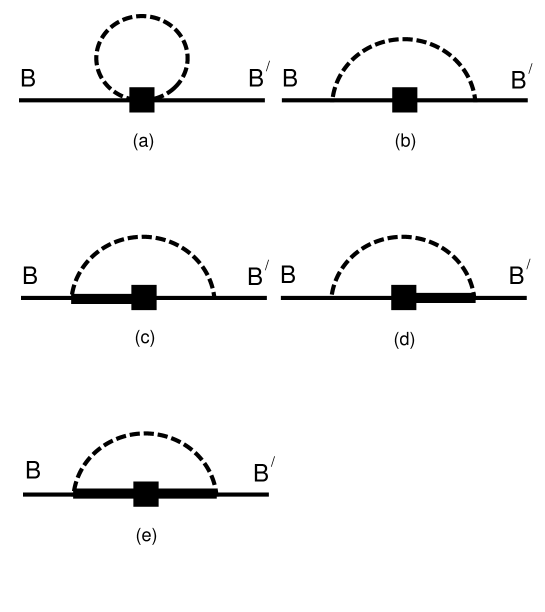
FIG. 2.: Loop-level contribution to the axial matrix element. The solid square denotes the insertion of the axial current. The labels $B$ and $B^{\prime}$ denote the incoming and outgoing octet baryons respectively. The dashed line denotes a pseudo-Goldstone boson. The thicker lines denote decuplet baryon propagators. Graphs of the type (a), (c) and (d) do not arise in the matrix element of the singlet current at one-loop.

FIG. 3.: Loop-level wavefunction renormalization contributions to the axial matrix element. The solid square denotes the insertion of the axial current. The labels $B$ and $B^{\prime}$ denote the incoming and outgoing octet baryons respectively. The dashed line denotes a pseudo-Goldstone boson. The thicker lines denote decuplet baryon propagators.

REFERENCES

• [1] D.B. Kaplan and A.V. Manohar, Nucl. Phys. B310 (1988) 527.
• [2] D. Adams et al (SMC collaboration), Phys. Lett. B357 (1995) 248.
• [3] R.L. Jaffe, hep-ph/9603422 (1996).
• [4] M. Musolf et al, Phys. Rep. 239 (1994) 1.
• [5] J. Lichenstadt and H.J. Lipkin, Phys. Lett. B353 (1995) 119.
• [6] B. Ehrnsperger and A. Schafer, Phys. Lett. B348 (1995) 619.
• [7] J. Dai et al, Phys. Rev. D53 (1996) 273.
• [8] R.L. Jaffe and A.V. Manohar, Nucl. Phys. B337 (1990) 509.
• [9] D. Adams et al (SMC collaboration), Phys. Lett. B329 (1994) 399; B339 (1994) 332 (E).
• [10] K. Abe et al (E143 Collaboration), Phys. Rev. Lett. 74 (1995) 346.
• [11] M. Prakash et al, Ap.J. L77 (1992) 390.
• [12] S. Reddy and M. Prakash, astro-ph/9610115, to appear in Ap.J. (1996).
• [13] J. Kodaira, Nucl. Phys. B165 (1979) 129.
• [14] S.L. Adler in “Lectures on Elementary Particle Physics and Quantum Field Theory”, ed. S. Deser, M. Grisaru and H. Pendelton (MIT Press, Cambridge, 1970).
• [15] A.V. Manohar, in “An Introduction to Spin Dependent Deep-Inelastic Scattering”, lectures presented at the Lake Louise Winter Institute (1992).
• [16] W. Koepf, E.M. Henley and S.J. Pollock, Phys. Lett. B288 (1992) 11.
• [17] M.J. Musolf and M. Burkardt, Z. Phys. C61 (1994) 433.
• [18] M. Ademollo and R. Gatto, Phys. Rev. Lett. 13 (1964) 264.
• [19] J. Anderson and M. Luty, Phys. Rev. D47 (1993) 4975.
• [20] E. Jenkins and A.V. Manohar, Phys. Lett. B255 (1991) 558.
• [21] E. Jenkins and A.V. Manohar, Phys. Lett. B259 (1991) 353.
• [22] E. Jenkins and A.V. Manohar, talk given at the workshop on ”Effective Field Theories of the Standard Model”, Dobogoko, Hungary (1991), ed. U. Meissner.
• [23] M.N. Butler, M.J. Savage and R.P. Springer, Nucl. Phys. B399 (1993) 69.
• [24] Particle Data Group, Phys. Rev. D54 (1996) 1.
• [25] E. Jenkins et al, Phys. Lett. B302 (1993) 482.
• [26] J. Dai et al, Phys. Lett. B271 (1991) 403.
• [27] D.B. Kaplan and M.J. Savage, Nucl. Phys. A556 (1993) 653; Nucl. Phys. A570 (1994) 833 (E).
• [28] E. Jenkins Nucl. Phys. B375 (1992) 561.
Refer to caption