This talk reviews some of the hot topics in spin physics and related subjects, including perturbative QCD predictions for polarized parton distributions and their possible behaviours at small $x$, the Bjorken and singlet sum rules and the treatment of higher orders in perturbative QCD, different interpretations of the EMC spin effect including chiral solitons and the axial $U(1)$ anomaly, other experimental indications for the presence of strange quarks in the nucleon wave function, implications for dark matter physics, and a few words about polarization as a tool in electroweak physics.

1   Introduction and Outline

Most of the talks at this meeting are concerned with spin phenomena in the strong interactions, and this emphasis is reflected in my talk, though I do have some words to say at the end about polarization in the electroweak interactions. Within QCD, we have a firm basis for understanding polarization effects in perturbative QCD, whereas it is a puzzle at the non-perturbative level which is linked to many fundamental issues in the theory. Among the non-perturbative phenomena that may be illuminated by polarization experiments are chiral symmetry breaking and the axial $U(1)$ anomaly. A bridge towards these non-perturbative effects may be provided by studies of higher orders in QCD perturbation theory. For example, renormalons may guide us in the identification of higher-twist and condensation phenomena in QCD. Spin physics is also linked to other interesting phenomena in particle physics, such as the question whether the proton wave function contains many strange quarks, which would have implications for the possible violations of the Okubo-Zweig-Iizuka (OZI) rule seen in recent experiments using the LEAR ring at CERN. Spin physics is also relevant to astrophysics and cosmology, since the couplings of dark matter particles, such as neutralinos and axions, to ordinary baryonic matter involves the same axial-current matrix elements that are measured in polarized-lepton-nucleon scattering experiments.

The theoretical interest of these experiments is mirrored by the intense experimental activity at many accelerator centres: CERN, SLAC, DESY, BNL, the Jefferson National Accelerator Facility formerly known as CEBAF, etc.. In this talk I will try to bring out the puzzles found by experimentalists to tease their theoretical colleagues, as well as the questions raised by theory that require further experimental elucidation. Spin physics is in a very active and exciting phase!

The outline of my talk is as follows: I first review our understanding of polarized partons in perturbative QCD, and flag their behaviour at small $x$ as a theoretical issue in NNLO perturbative QCD that could be clarified by data at HERA with a polarized proton beam. Then I discuss the evaluation of QCD sum rules for polarized structure functions, addressing the issues of the $Q^{2}$-dependence of the polarization asymmetry, where deep-inelastic $\nu$-nucleon collisions could cast some light, and the resummation of higher orders in QCD perturbation theory, which may be tackled using Padé approximants. Next, I emphasize that the interpretation of the EMC spin effect is an open issue in non-perturbative QCD, with chiral solitons and non-perturbative $U_{A}(1)$ dynamics as competing explanations that require experiments to distinguish them. Here HERMES, COMPASS, polarized RHIC and polarized HERA may be able to contribute via determinations of the gluon polarization $\Delta G$. On the other hand, experiments on the “violation” of the OZI rule and final-state measurements in deep-inelastic lepton scattering may cast some light on the possible existence and polarization of strange quarks and antiquarks in the nucleon wave function. Finally, after advertizing the connection between polarization experiments and searches for non-baryonic dark matter, I close with praise for the rôle played by spin physics in the electroweak sector, including precision measurements at the $Z^{0}$ peak at both LEP and the SLC that suggest a mass range for the Higgs boson within reach of forthcoming experiments at LEP 2 or at the LHC.

2   Polarized Partons in Perturbative QCD

Since I am the first speaker at this meeting, it seems that I must introduce the two polarized structure functions $G_{1,2}(\nu,Q^{2})$ that form the basis [1] for many of the discussions in this talk and during the meeting:

$$\frac{d^{2}\sigma^{\uparrow\downarrow}}{dQ^{2}d\nu}-\frac{d^{2}\sigma^{\uparrow\uparrow}}{dQ^{2}d\nu}=\frac{4\pi\alpha^{2}}{Q^{2}E^{2}}\left[m_{N}(E+E^{\prime}\cos\sigma)G_{1}(\nu,Q^{2})-Q^{2}G_{2}(\nu,Q^{2})\right]$$ (1)

In the Bjorken scaling limit $Q^{2}\rightarrow\infty,x\equiv Q^{2}/2m_{N}\nu$ fixed, according to the naive parton model:

$$m^{2}_{N}\nu G_{1}{\nu,Q^{2}}\rightarrow g_{1}(x),\,m_{N}\nu^{2}G_{2}(\nu,Q^{2})\rightarrow g_{2}(x)$$ (2)

The dominant $g_{1}(x)$ structure function is related in the naive parton model to polarized quark distributions:

$$g_{1}^{p}(x) = \frac{1}{2}\sum_{q}e^{2}_{q}\left[q_{\uparrow}(x)-q_{\downarrow}(x)+\bar{q}_{\uparrow}(x)-\bar{q}_{\downarrow}(x)\right]$$ (3)

$$= \frac{1}{2}\sum_{q}e^{2}_{q}\Delta q(x)$$

whereas the unpolarized structure function $F_{2}(x)$ is given by:

$$F_{2}(x)=\sum_{q}e^{2}_{q}x\left[q_{\uparrow}(x)+q_{\downarrow}(x)+\bar{q}_{\uparrow}(x)+\bar{q}_{\downarrow}(x)\right]$$ (4)

Polarized lepton-nucleon scattering experiments actually measure directly the polarization asymmetry $A_{1}$ related to the virtual-photon absorption cross sections $\sigma_{1/2,3/2}$:

$$A_{1}\equiv\frac{\sigma_{\frac{1}{2}}-\sigma_{\frac{3}{2}}}{\sigma_{\frac{1}{2}}+\sigma_{\frac{3}{2}}}\rightarrow\frac{\sum_{q}e^{2}_{q}\left[q_{\uparrow}(x)-q_{\downarrow}(x)+...\right]}{\sum_{q}e^{2}_{q}\left[q_{\uparrow}(x)+q_{\downarrow}(x)+...\right]}$$ (5)

I will not address here the interesting issues related to the transverse asymmetry $A_{2}$, but move straight on to discuss the perturbative evolution of the polarized structure functions.

As $Q^{2}$ increases, the standard GLAP perturbative evolution equations [2] take the form

$$g_{1}(x,t) = \frac{1}{2}<e^{2}>\int^{1}_{x}\frac{dy}{y}\times$$ (6)

$$\times \left[C^{S}_{q}\left(\frac{x}{y},\alpha_{s}(t)\right)\Delta\Sigma(y,t)+2N_{f}C_{g}\left(\frac{x}{y},\alpha_{s}(t)\right)\Delta G(y,t)\right.$$

$$+ \left.C^{NS}_{q}\left(\frac{x}{y},\alpha_{s}(t)\right)\Delta q^{NS}(y,t)\right]$$

where $t\equiv\hbox{ln}(Q^{2}/\Lambda^{2})$, the $C_{i}(x/y,\alpha_{s}(t))$ are coefficient functions, $\Delta\Sigma(y,t)$ is the singlet combination of the $\Delta q(y,t)$, and $\Delta q^{NS}(y,t)$ is a non-singlet combination. The polarized parton distributions obey coupled integro-differential equations of the form

$$\frac{d}{dt}\left(\begin{array}[]{ll}\Delta\Sigma(y,t)\\ \Delta G(y,t)\end{array}\right) = \frac{\alpha_{s}(t)}{2\pi}\int^{1}_{x}\frac{dy}{y}\left(\begin{array}[]{lr}P^{S}_{qq}&2N_{f}P_{qq}\\ P_{gq}&P_{gg}\end{array}\right)\left(\begin{array}[]{l}\Delta\Sigma\\ \Delta G\end{array}\right)$$ (13)

$$\frac{d}{dt}\Delta q^{NS}(y,t) = \frac{\alpha_{s}(t)}{2\pi}\int^{1}_{x}\frac{dy}{y}P^{NS}_{qq}\left(\frac{x}{y},\alpha_{s}(t)\right)\Delta q^{NS}(y,t)$$ (14)

where the $P_{ij}(x/y,\alpha_{s}(t))$ are polarized splitting functions. At leading order in $\alpha_{s}(t)$, $C_{q}=1,C_{g}=0,P_{ij}={\cal O}(1)$ [3]. Recently, thanks to heroic efforts by local industry in particular [4], we now know the NLO corrections $\delta(C,P)={\cal O}(\alpha_{s}/\pi)$. The exact way in which these NLO corrections are divided up between the polarized quark and gluon distributions is renormalization-scheme dependent, as we shall review later. There is much discussion at this meeting of NLO QCD fits fits to polarized structure function data: one state-of-the-art fit [5] is shown in Fig. 1.

Figure 1: One state-of-the-art NLO perturbative QCD fit to polarized structure function data, including lines showing the behaviours at two fixed values of $Q^{2}$, and at the $x$-dependent values appropriate to different experiments [5].

One area where further guidance should be sought from perturbative QCD, as well as information from experiment, is the low-$x$ region. Before perturbative QCD came on the scene, the only guidance came from Regge theory [6], which suggested that

$$g_{1}^{p,n}\simeq x^{-\alpha}$$ (15)

where the intercept $\alpha$ of the relevant axial-vector meson trajectory was guessed to lie in the range $0\geq\alpha\geq-0.5$. Data on the effective Pomeron intercept from HERA suggest that this might be appropriate for $Q^{2}<1$ GeV², but that perturbative QCD plays an essential rôle at higher $Q^{2}$. Standard resummation of the GLAP $Q^{2}$ logarithms $\Sigma_{n,m}\alpha_{s}(t)^{n}(\hbox{ln}Q^{2})^{m}$ suggests [7] that

$$\left(\ell n|\frac{1}{x}|\right)^{p}<<g_{1}^{p,n}(x)<<x^{-q}$$ (16)

for any positive $p,q$. However, a BFKL-inspired resummation of $1/x$ logarithms $\Sigma_{n,m}\alpha_{s}(t_{0})^{n}(\hbox{ln}1/x)^{m}$ at fixed $Q_{0}^{2}$ suggests [8] that

$$g_{1}(x,Q^{2})^{NS}\sim x^{-0.4}\left(\frac{Q^{2}}{\mu^{2}}\right)^{0.2},g_{1}(x,Q^{2})^{S}\sim x^{-1..0}\left(\frac{Q^{2}}{\mu^{2}}\right)^{0.5}$$ (17)

where we see that the singlet combination of structure functions dominates the non-singlet at small $x$. BFKL behaviour is not required by the unpolarized HERA data [9], and singlet dominance is not indicated by the SMC polarized data [5] at the lowest available $x$. There is some discussion here of preliminary data from the SLAC E154 experiment, which can be fit by a power law: $g_{1}^{n}\sim x^{-0.8}$ for $0.02<x<0.1$, but these data are at $Q^{2}$ too low, and $x$ too high, for equation (11) to be applicable.

It has been shown that the resummation of the leading higher-order corrections is important for the singlet combination of polarized structure functions, which is very sensitive to their treatment [10]. This is still an important source of systematic error, which could only be reduced significantly by tough theoretical calculations (NNLO, singular terms at higher orders), and/or by measurements at polarized HERA [11]..

3   Sum Rules

Defining the integrals $\Gamma_{1}^{p,n}\equiv\int_{0}^{1}g_{1}^{p,n}$, one has at the parton level the Bjorken [12] sum rule

$$\Gamma_{1}^{p}\,-\Gamma_{1}^{n}=\frac{1}{6}g_{A}=\Delta u-\Delta d$$ (18)

whereas one can derive sum rules for the individual integrals

$$\Gamma_{1}^{p,n}=\left(\pm\frac{1}{12}g_{A}+\frac{1}{36}a_{8}\right)+\frac{1}{9}\Delta\Sigma$$ (19)

where $a_{8}\equiv(\Delta u+\Delta d-2\Delta s)/\sqrt{3}$, only if one assumes that $\Delta s=0$ [13], implying for example that

$$\Gamma_{1}^{p}\simeq 0.19$$ (20)

The justification for this assumption was never very strong: to paraphrase Ref. [13], “probably there are no strange quarks in the proton wave function, and if there are, surely they are not polarized”.

The sum rules (12) and (13) acquire significant subasymptotic corrections in perturbative QCD [14]:

$$\Gamma_{1}^{p}(Q^{2})-\Gamma_{1}^{n}(Q^{2}) = \frac{1}{6}g_{A}\left[1-\frac{\alpha_{s}(Q^{2})}{\pi}-3.5833\left(\frac{\alpha_{s}(Q^{2})}{\pi}\right)^{2}\right.\hfill$$

$$\left.-20.2153\left(\frac{\alpha_{s}(Q^{2})}{\pi}\right)^{3}-0(130)\left(\frac{\alpha_{s}}{\pi}\right)^{4}+\ldots\right]\phantom{xxxxxxxxx}{(15a)}$$

$$\Gamma^{p,n}_{1}(Q^{2}) = \left(\pm\frac{1}{12}g_{A}+\frac{1}{36}a_{8}\right)\left[1-\frac{\alpha_{s}(Q^{2})}{\pi}-3.5833\left(\frac{\alpha_{s}(Q^{2})}{\pi}\right)^{2}\right.\hfill$$

$$\left.-20.2153\left(\frac{\alpha_{s}(Q^{2})}{\pi}\right)^{3}-0(130)\left(\frac{\alpha_{s}}{\pi}\right)^{4}\right]+\frac{1}{9}\Delta\Sigma\hfill$$

$$\left[1-\frac{\alpha_{s}(Q^{2})}{\pi}-1.0959\left(\frac{\alpha_{s}(Q^{2})}{\pi}\right)^{2}-0(4)\left(\frac{\alpha_{s}(Q^{2})}{\pi}\right)^{3}+\ldots\right]\phantom{xxxx}{(15b)}$$

where the highest-order terms are estimates [15], leading, for example, to the prediction that, if $\Delta s=0$, $\Gamma_{1}^{p}\simeq 0.17$ at a $Q^{2}$ typical of the EMC experiment [16].

Sometimes there is still discussion of testing the Bjorken sum rule. This is an absolutely fundamental prediction of QCD that has (in my opinion) by now been tested successfully: for me, the issue is now to use the subasymptotic corrections in the Bjorken sum rule (15a) to determine $\alpha_{s}(Q^{2})$ [17,18]. Using the subasymptotic corrections in (15b), one may check whether $\Delta s=0$, or measure its value. A non-zero value is no “crisis” for perturbative QCD, just a surprise for overly naive models of non-perturbative QCD matrix elements.

One of the issues to be confronted in testing these sum rules is that the data are not all taken at the same $Q^{2}$, and some interpolation/extrapolation is necessary to evaluate $\Gamma_{1}^{p,n}(Q^{2})$. Experimentally, this is usually done by assuming that $A_{1}$ or $g_{1}/F_{1}$ is independent of $Q^{2}$, which seems empirically to be true [5] within the errors for $Q^{2}\mathrel{\hbox to0.0pt{\raise 2.15277pt\hbox{$>$}\hss}{\lower 2.15277pt\hbox{$\sim$}}}1$ GeV². Theoretically, there is no reason why this should be true [7], although substantial deviations are not expected for $x\mathrel{\hbox to0.0pt{\raise 2.15277pt\hbox{$>$}\hss}{\lower 2.15277pt\hbox{$\sim$}}}0.1$. For larger $x$, the form of the expected scaling violations is identical to NLO to those in $xF_{3}(\nu N)$, and it may be possible to use deep-inelastic $\nu N$ data to give hints how to interpolate/extrapolate polarized $\ell N$ data where these are incomplete.

The experimental determinations of the $\Gamma_{1}^{p,d}$ are compiled in Fig. 2: things look grim for the singlet sum rules, but let us first discuss quantitatively the Bjorken sum rule.

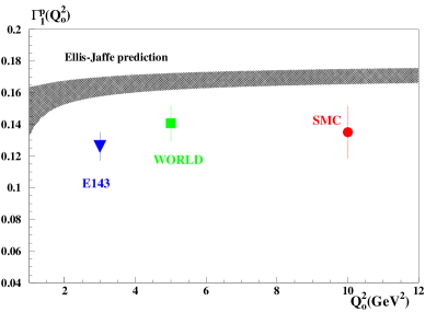
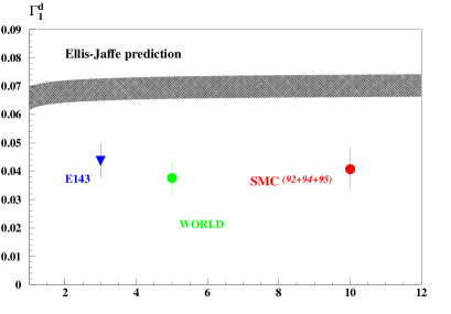
Figure 2: A compilation [5] of measurements of the integrals $\Gamma_{1}^{p,d}(Q^{2})$, showing significant disagreement with the singlet sum rule predictions [13].

It is apparent from (15) that one of the issues that must be addressed is the treatment of higher orders of QCD perturbation theory [18]. A generic QCD perturbation series is expected to be asymptotic:

$$S(x)=\sum^{\infty}_{n=0}\,c_{n}x^{n}\,:\,x\equiv\frac{\alpha_{s}}{\pi},c_{n}\simeq n!K^{n}n^{\gamma}$$ (22)

corresponding to the presence of one or more renormalon singularities. Confronted with an asymptotic series, one normally calculates it up to the “optimal” order $n_{opt}\equiv n:\Delta_{n}(x)\equiv|c_{n}x^{n}|$ is minimized, and then stops, quoting $\Delta_{n_{opt}}$ as an error estimate. Looking at the series in (15), it seems that we have not yet reached $n_{opt}$ for $\alpha_{s}/\pi\mathrel{\hbox to0.0pt{\raise 2.15277pt\hbox{$<$}\hss}{\lower 2.15277pt\hbox{$\sim$}}}1$. Is there some way of estimating the next terms in the series, and of resumming the series so as to minimize the estimated error?

One approach is to use Padé approximants:

$$[N/M]=\frac{a_{0}+a_{1}x+\ldots a_{N}x^{N}}{1+b_{1}x+\ldots b_{M}x^{M}}\,:\,[N/M]=S+O(x^{N+M+1})$$ (23)

which are known to give good estimates in other applications [19], and have been proven to converge if $\epsilon_{n}\equiv(c_{n}c_{n+2}/c^{2}_{n+1})-1\simeq{\cal O}(1/n)$, which is known to be the case for series dominated by a finite number of renormalon poles [18]. We then predict that

$$\ell n|\delta_{[M/M]}|\simeq-M[1+\ell n(2+a)]:\delta_{[N/M]}\equiv\frac{c^{est}_{N+M+1}-c_{N+M+1}}{c_{N+M+1}}$$ (24)

where $a$ is some number. This prediction is verified [1] for the QCD vacuum polarization evaluated in the limit $N_{f}\rightarrow\infty$, as seen in Fig. 3. Applied to the first three terms in (15a), the $[1/2]$ and $[2/1]$ Padé approximants yield [18] the estimate $c_{4}\simeq-112\pm 33$, to be quoted with the effective charge estimate $c_{4}\simeq-130$.

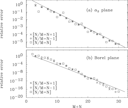
Figure 3: The errors in Padé approximant predictions for the perturbative expansion coefficients for the QCD vacuum polarization $D$ function in the large-$N_{f}$ approximation, compared with theoretical error estimates (18,20) [1].

As seen in Fig. 3, the convergence of the Padé approximants is even better [18,19] when one makes a Borel transform of the perturbative QCD series:

$$\tilde{S}(y)\equiv\sum^{\infty}_{n=0}\,\tilde{c}_{n}y^{n}\,:\,\tilde{c}_{n}\equiv\frac{c_{n+1}}{n!}\left(\frac{4}{\beta_{o}}\right)^{n+1}\,:\,\beta_{0}\equiv\frac{(33-2N_{f})}{3}$$ (25)

This is because ${\tilde{\epsilon}}_{n}\equiv({\tilde{c}}_{n}{\tilde{c}}_{n+2}/{\tilde{c}}_{n+1}^{2})-1\simeq 1/n^{2}$, implying that

$$\ell n|\tilde{\delta}_{[M/M]}|\simeq-2M[1+\ell n(2+a)]$$ (26)

as seen [1] in the second panel of Fig. 3. Indeed, if the series is dominated by a finite set of renormalon poles, the Padé approximants become exact. In the case of the series (15a) for the Bjorken sum rule, the $[2/1]$ Padé approximant in the Borel plane has a pole at $y=1.05$, to be compared with the expected renormalon singularity at $y=1$ [17].

Further evidence for the reliability of Padé approximants is provided by studies of the renormalization scale and scheme dependences of the Padé resummation of the perturbative QCD series for the Bjorken sum rule. We recall that the full “sum” is a measurable quantity that should be independent of renormalization scale: $\partial/\partial\mu=0$, and similarly of the scheme ambiguity parametrized by $c_{2}$ at NLO: $\partial/\partial c_{2}=0$. Fig. 4 shows that the Padé estimate of the sum is much less scale dependent than partial sums of the QCD perturbation series [18], and Fig. 5 shows that it also has very little renormalization-scheme dependence [20].

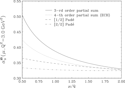
Figure 4: The renormalization scale dependence of the Bjorken sum rule is greatly reduced by the use of Padé approximants [18].

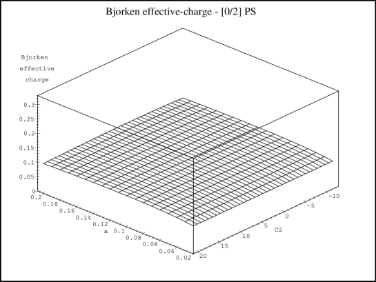
Figure 5: The renormalization scheme dependence of the Bjorken sum rule is also greatly reduced by the use of Padé approximants [20].

We have used [20] the data available before this meeting in a numerical analysis of the Bjorken sum rule, using Padé approximants to sum the QCD perturbation series. We took the data at face value, accepting the experimental estimates of their extrapolations to small $x$, and of the associated systematic errors. We do not expect this extrapolation to be very badly behaved for non-singlet combinations of structure functions, such as appear in the Bjorken sum rule. Combining the experimental numbers, we find $\Gamma_{1}^{p}-\Gamma_{1}^{n}=0.160\pm 0.014$ at $Q^{2}=3$ GeV², corresponding to

$$\alpha_{s}(M_{z})=0.117^{+0.004}_{-0.007}\pm 0.002$$ (27)

when using Padé summation [20], where the first error is experimental, and the second is a theoretical error associated with the residual renormalization-scheme dependence in Fig. 5. This compares well with the world average quoted at the Warsaw conference [21]: $\alpha_{s}(M_{Z})=0.118\pm 0.003$, and the consistency implies that the Bjorken sum rule is verified at the $10\%$ level.

x

We already saw in Fig. 2 that the singlet sum rules do not fare too well. All the data are highly consistent if all the perturbative QCD corrections in (15) are taken into account [1]: this would not be apparent for the neutron data if one did not include all the corrections. A global fit to the data indicates that

$$\Delta u = 0.81\pm 0.01\pm,\;\Delta d=-0.44\pm 0.01\pm,$$

$$\Delta s = -0.10\pm 0.01\pm,\;\Delta\Sigma=0.27\pm 0.04\pm$$ (28)

at $Q^{2}=3$ GeV². The second $\pm$ signs in (22) represent further sources of error, including higher twists and the possible $Q^{2}$-dependence of $A_{1}$, but principally the low-$x$ extrapolation. As already mentioned, this is very sensitive to the treatment of higher-order perturbative QCD terms. Considerably more theoretical and experimental work is necessary before the second errors in (22) can be reduced to the level of the first ones. Nevertheless, it is clear that $\Delta s\neq 0$ and that $\Delta\Sigma<<1$, in disagreement with naive quark model estimates.

4   Interpretations of the EMC Spin Effect

Chiral Soliton (Skyrmion): CQCD has a large chiral symmetry : $q_{L(R)}\rightarrow L(R)q_{L(R)}$, which has an $SU(N_{f})\times SU(N_{f})\times U(1)_{B}$ group structure that is broken spontaneously by non-perturbative vacuum expectation values $<O|\bar{q}_{L}\bar{q}_{R}+h.c.|0>$ that couple the left $(L)$ and right $(R)$ helicities [22]. We discuss later the fate of the axial $U(1)$ factor: it is broken by an amount $O(1/N_{c})$. This spontaneous symmetry breakdown is accompanied by the appearance of an octet of light pseudo-Goldstone bosons $\pi^{\pm,0},K^{\pm,0,\bar{0}},\eta_{8}$, but not the singlet $\eta_{0}$ that disappears along with the axial $U(1)$ current: it decouples as $N_{c}\rightarrow\infty$. There is a simple effective Lagrangian [22]

$${\cal L}_{\pi}=\frac{f^{2}_{\pi}}{16}\,Tr(\partial_{\mu}U\partial^{\mu}U^{\dagger})+\ldots:U\equiv\mbox{exp}\left[\frac{2i}{f_{\pi}}\underline{\pi}\cdot\underline{\tau}\right]$$ (29)

that describes their dynamics at energies $E<<\Lambda_{QCD}$ or distances $R>>1/\Lambda_{QCD}$ in the limit that $m_{u,d,s}<<\Lambda_{QCD}$. This Lagrangian (22) has classical soliton (lump) solutions $U(\underline{x})$ [23] that are labelled by the group $\pi_{3}(SU(N_{f}))={\bf Z}$, where the integers count the baryon number $B$ that may be represented by

$$B=\frac{1}{24\pi^{2}}\,\epsilon_{ijk}\,\int d^{3}\underline{x}\,Tr(\partial_{i}UU^{\dagger}\partial_{j}UU^{\dagger}\partial_{k}UU^{\dagger})$$ (30)

The lowest-lying state has $B=1$ and may always be quantized as a fermion.

Axial-current matrix elements in this model are given via PCAC by generalized Goldberger-Treiman relations to the couplings of the corresponding light mesons $\pi^{\pm,0},K^{\pm,0,\bar{0}},\eta_{8}$. There is no singlet axial-current coupling because there is no singlet meson $\eta_{0}$ in the Lagrangian: the soliton is a “lump” of octet fields, and the $\eta_{0}$ decouples in the large-$N_{c}$ limit, in which [24]

$$\Delta\Sigma=\Delta u+\Delta d+\Delta s=0,$$ (31)

and there is also no way to obtain $\Delta G\neq 0$.

In the chiral soliton model, the nucleon spin arises [24] from the quantization of the classical “lump”, and is interpreted as due to a coherent rotation of the cloud of $\pi,K$ and $\eta_{8}$ mesons : $L_{z}=\frac{1}{2}$. In the quark language, the baryons are viewed as coherent states of a very large number of light, relativistic quarks. In the real world with $N_{c}=3$ and $m_{u,d,s}\not=0$, we do not expect (25) to be exact, but it might be accurate at the $O(1/N_{c})\simeq 30\%$ level, as indicated by the experimental determination (22).

Alternative approaches are based on the axial $U(1)$ anomaly, which contributes [25] to the perturbative evolution of the polarized parton distributions at NLO:

$$<p|\bar{q}\gamma_{\mu}\gamma_{5}q|p>=2S_{\mu}\left(\Delta q^{LO}-\frac{\alpha_{s}}{2\pi}\Delta G^{LO}\right)$$ (32)

As already mentioned, there is some freedom of renormalization-scheme choice at NLO, and the $\overline{MS}$ option is simply to absorb the $\Delta G^{LO}$ correction in (26) into the definition of $\Delta q$ at NLO: $\Delta q\equiv\Delta q^{LO}-\frac{\alpha_{s}}{2\pi}\Delta G^{LO}$. Alternatively, one may keep the $\Delta G^{LO}$ correction separate: $\Delta q,G^{LO}=\Delta q,G$, in which case $\Delta\Sigma=\Delta u+\Delta d+\Delta s-\frac{3\alpha_{s}}{2\pi}\Delta G$. One can then hope to save the original assumption that $\Delta s=0$ by postulating that the apparent non-zero value of $\Delta s$ in (22) is in fact due to the $\Delta G$ correction, and that $\Delta u+\Delta d+\Delta s$ is correctly predicted by the naive non-relativistic quark model, with the small observed value of $\Delta\Sigma$ also due to the $\Delta G$ correction. This would require a rather large positive value of $\Delta G$, which would need to be compensated by a correspondingly large negative value of $L_{z}$. Note that this axial-anomaly interpretation [25] does not predict the measured values of $\Delta s$ and $\Delta G$ without an extra dynamical assumption .

The first attempt to measure $\Delta G$ directly was in a Fermilab experiment [27] looking for a particle-production asymmetry in polarized $pp$ collisions. Their measurements indicate that $\Delta G$ may even be negative , though they are not very conclusive, because of the statistical and systematic limitations of the experiment. There have recently been several attempts [29] to extract $\Delta G$ indirectly from scaling violations in polarized structure functions. These hint that $\Delta G>0$, and are mostly consistent with $\Delta G=O(1)$. However, the numerical value is still unknown: uncertainties are still large, and do not yet permit even an unambiguous measurement of the sign of $\Delta G$. This is the task entrusted to new experiments such as HERMES, COMPASS, polarized RHIC and polarized HERA.

5   “Breaking” the Okubo-Zweig-Iizuka Rule

According to this rule [30], one should draw diagrams with connected quark lines, and disconnected diagrams require gluon exchanges and should be suppressed. The only “breaking” of the rule for $\phi$ and $f^{\prime}_{2}$ meson production is blamed on the small $\bar{u}u+\bar{d}d$ components in their wave functions. The rule works well for mesons, but there is no good evidence that it works well for baryons. For example, if one estimates the $\pi$-nucleon $\sigma$ term $\Sigma^{\pi N}=\frac{1}{2}(m_{u}+m_{d})<p|(\bar{u}u+\bar{d}d)|p>$ using the Gell-Mann-Okubo mass formula and the dynamical assumption that $<p|\bar{s}s|p>=0$, one finds $\Sigma^{\pi N}\simeq 25$ MeV, to be compared with the value $\Sigma^{\pi N}\simeq 45$ MeV inferred from experiment [31]. This corresponds to

$$\frac{<p|\bar{s}s|p>}{<p|(\bar{u}u+\bar{d}d+\bar{s}s)|p>}\simeq 0.2$$ (33)

Likewise, the polarized structure function data (22) indicate that $<p|\bar{s}\gamma_{\mu}\gamma_{5}s|p>\not=0$, as do data [32] on elastic $\bar{\nu}p\rightarrow\bar{\nu}p$ scattering .

Confirming earlier suggestions [33], recent data from experiments at LEAR find large apparent violations of the OZI rule in $\bar{p}N$ annihilation at rest . The production ratios $\phi X/wX$ for $X=\pi^{\pm,0},\pi\pi$ and $\gamma$ all exceed the OZI predictions, in some cases by as much as a factor of 100! Moreover, there are indications that this OZI violation is spin-dependent, since it is large in $S$-wave annihilations, but not in $P$-wave annihilations, as seen in Fig. 6.

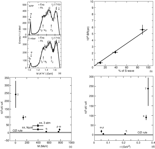
Figure 6: The $\phi$ production [35] in ${\bar{p}}N$ annihilation (a) depends on the way in which the initial state is prepared, corresponding (b) to a large enhancement of production in the $S$-wave annihilations favoured at NTP. It also depends (c) on the final-state particle with which the $\phi$ is produced, and (d) on the momentum transfer. These are all features that models [36] need to explain.

One interpretation [33,36] of these data is that they are due to OZI evasion, rather than breaking. If the proton wave function contains $\bar{s}s$ pairs, there are additional connected quark-line diagrams that can be drawn, giving enhanced $\phi$ production. Such an $\bar{s}s$ component may also explain the backward peak seen in the $\bar{p}p\rightarrow K^{-}K^{+}$ reaction. Detailed models [36] agree qualitatively with the pattern of OZI “breaking” seen in the LEAR experiments. Other interpretations of the apparent OZI “breaking” include rescattering by intermediate $K$ and $K^{*}$ states, but this is subject to systematic cancellations and does not seem to explain the initial-state dependence that has been seen. There is also no trace of an exotic resonance postulated in another interpretation of early data on OZI “breaking”.

The proposition that the proton wave function contains $\bar{s}s$ pairs, and that they are polarized, can be tested by looking for $\Lambda$ polarization in the target fragmentation region of deep-inelastic $\nu,e$ or $\mu N$ scattering [37]. The idea is that the $\nu$ or polarized $e,\mu$ selects preferentially one parton polarization in the proton wave functions, e.g., a $u^{\uparrow}$. The proton remnant should remember the polarization of the struck parton, and in particular one might expect negative $s$ polarization: $|p>\ni u^{\uparrow}(\bar{s}s)_{\downarrow}+\ldots$. Memory of this $s$ polarization may well be transferred with a dilution factor $D$ to any $\Lambda$ in the current fragmentation: $s_{\downarrow}\rightarrow\Lambda_{\downarrow}$. Such $\Lambda$ polarization was indeed seen in the WA59 $\bar{\nu}N$ experiment [38]: for $0.2<x<1$, $P_{\Lambda}=-0.85\pm 0.19$ to be compared with a postdiction $P_{\Lambda}=-0.94D$, indicating that $D=0.9\pm 0.2$. This model can be used to make predictions for polarized $e(\mu)N$ scattering: $P_{\Lambda}=0.7P_{\mu}D$, which should be observable in the HERMES and COMPASS experiments.

It would be interesting to know whether polarized-gluon models have anything to say about OZI “breaking” or $\Lambda$ polarization experiments.

6   Spin-off for Dark Matter Particles

Polarization experiments are relevant to astrophysics and cosmology, as we now discuss. One of the favoured candidates for cold dark matter is the lightest neutralino $\chi$, which has spin-dependent couplings with nucleons that would be responsible for its capture by the Sun (which could be detected by high-energy solar neutrinos produced by $\chi\chi$ annihilation), and would contribute to elastic $\chi$ scattering off nuclei in the laboratory (which could be used to detect dark-matter $\chi$ particles directly). The spin-dependent matrix element $M$ contributing to $\sigma(\chi p\rightarrow\chi p)$ is related to axial-current matrix elements [39]. In particular, if the $\chi$ particle is approximately a photino

$$M\simeq\sum_{q}e^{2}_{q}\Delta q$$ (34)

which is exactly the linear combination measured in polarized deep-inelastic $(e,\mu)p$ scattering experiments: have EMC et al. been measuring elastic $\chi p$ scattering?

Another popular cold dark matter candidate is the axion, a very light pseudoscalar boson:

$$m_{a}\propto m^{2}_{\pi}/f_{a},\;g_{aff}\propto m_{f}/f_{a},\;g_{a\gamma\gamma}\propto 1/f_{a}$$ (35)

where $f_{a}$ is a decay constant analogous to $f_{\pi}$, which was postulated to ensure CP conservation in the strong interactions. Accelerator experiments tell us that $f_{a}\mathrel{\hbox to0.0pt{\raise 2.15277pt\hbox{$>$}\hss}{\lower 2.15277pt\hbox{$\sim$}}}1$ TeV, and coherent axion waves could contribute a significant fraction of the mass density of the Universe if $f_{a}\sim 10^{11}$ to $10^{12}$ GeV. There are many astrophysical bounds on $f_{a}$ which depend on the axion-nucleon couplings $C_{ap,an}$. These are related by generalized Goldberger-Treiman relations to axial-current matrix elements [40]:

$$C_{ap} = 2(-2.76\Delta u-1.13\Delta d+0.89\Delta s)-\cos 2\beta(\Delta u-\Delta d-\Delta s)$$

$$C_{an} = 2(-2.76\Delta d-1.13\Delta u+0.89\Delta s)-\cos 2\beta(\Delta d-\Delta u-\Delta s)$$ (36)

where $\cos 2\beta$ is related to an unknown ratio of Higgs v.e.v.’s. Using (29), one can determine the supernova axion emission rate, which is $\propto C^{2}_{an}+0.8(C_{an}+C_{ap})^{2}+C^{2}_{ap}$, as seen in Fig. 7. The determinations (21) of the $\Delta q$ determine [17] the $C_{ap,an}$ with errors that are smaller than many other astrophysical uncertainties, such as the equation of state inside a supernova core. Reconciling the axion emission rate with observations of neutrinos emitted by supernova SN1987a is possible only if $f_{a}\mathrel{\hbox to0.0pt{\raise 2.15277pt\hbox{$>$}\hss}{\lower 2.15277pt\hbox{$\sim$}}}10^{10}$ GeV [40]. This is a second example of the importance of polarization experiments for astrophysics and cosmology.

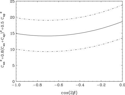
Figure 7: The axion emission rate from a supernova core is roughly proportional to the scale on the vertical axis. Determinations of the $\Delta q$ now constrain it with the uncertainty indicated by the dot-dashed curves [17], which is considerably smaller than other uncertainties associated with modelling the nuclear equation of state.

7   Polarization in Electroweak Physics

Although most of this meeting is concerned with spin phenomena in the strong interactions, I cannot resist saluting briefly the importance of polarization in electroweak physics. Transverse beam polarization has been an invaluable tool for calibrating the LEP beam energy and hence measuring accurately the $Z^{0}$ mass. One of the most precise determinations of the electroweak mixing parameter $\sin^{2}\theta_{W}$ is the left-right production asymmetry measured using longitudinal beam polarization at the SLC [41]. Other important measurements of $\sin^{2}\theta_{W}$ are made using $\tau$ polarization measurements. Precision electroweak measurements enabled the top quark mass to be predicted on the basis of radiative corrections. They are now able to predict [42] the Higgs boson mass with a factor of 2 error:

$$M_{H}=145^{+164}_{-77}~{}~{}~{}~{}GeV$$ (37)

as seen in Fig. 8. Perhaps future electroweak polarization measurements will enable us to refine further this prediction. If this prediction is confirmed by observation of the Higgs boson, electroweak polarization will indeed have realized its rosy prospects!

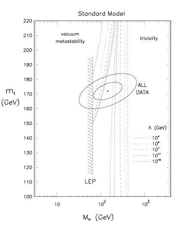
Figure 8: The $1$- and $2-\sigma$ predictions [42] for $M_{H},m_{t}$ based on precision electroweak data, confronted with the LEP lower limit and the ranges predicted if the Standard Model is assumed to remain valid up to different cutoff scales $\Lambda$.

[1] For a review and references, see J. Ellis and M. Karliner, CERN-TH/95-334.

[2] V.N. Gribov and L.N. Lipatov, Yad. Fiz. 15 (1972) 781 [Sov. J. Nucl. Phys. 15 (1972) 438];
G. Altarelli and G. Parisi, Nucl. Phys. B125 (1977) 298.

[3] K. Sasaki, Prog. of Theor. Phys. 54 (1975) 1816;
M.A. Ahmed and G.G. Ross, Nucl. Phys. B111 (1976) 441.

[4] E.B. Zijlstra and W.L. van Neerven, Nucl. Phys. B417 (1994) 61; Erratum B426 (1994) 245;
R. Mertig and W.L. van Neerven, Z. Phys. C70 (1996) 637;
W. Vogelsang, Phys. Rev. D54 (1996) 2023, RAL-TR-96-020;
R. Hamberg and W.L. van Neerven, Nucl. Phys. B379 (1992) 143.

[5] G. Mallot, talk at this meeting;
SMC collaboration, D. Adams et al., in preparation.

[6] R.L. Heimann, Nucl. Phys. B64 (1973) 429;
J. Ellis and M. Karliner, Phys. Lett. B213 (1988) 73.

[7] R.D. Ball, S. Forte and G. Ridolfi, Phys. Lett. B378 (1996) 255.

[8] J. Bartels, B.I. Ermolaev and M.G. Ryskin, “Non-singlet contributions to the structure function $g_{1}$ at small $x$”, hep-ph/9507271.

[9] R.D. Ball and S. Forte, Nucl. Phys. B444 (1995) 287; E-ibid. B449 (1995) 680.

[10] J. Blümlein and A. Vogt, DESY-96-050 (hep-ph/9606254).

[11] A. Schäfer, talk at this meeting.

[12] J. Bjorken, Phys. Rev. 148 (1966) 1467; D1 (1970) 1376.

[13] J. Ellis and R.L. Jaffe, Phys. Rev. D9 (1974) 1444; D10 (1974) 1669.

[14] J. Kodaira et al., Phys. Rev.D20 (1979) 627;
J. Kodaira et al., Nucl. Phys. B159 (1979) 99;
S.A. Larin, F.V. Tkachev and J.A.M. Vermaseren, Phys. Rev. Lett. 66 (1991) 862;
S.A. Larin and J.A.M. Vermaseren, Phys. Lett.B259 (1991) 345;
S.A. Larin, Phys. Lett.B334 (1994) 192.

[15 A.L. Kataev and V.S. Starshenko, Mod. Phys. Lett. A10 (1995) 235.

[16] The EMC Collaboration, J. Ashman et al., Phys. Lett. B206 (1988) 364; Nucl. Phys. 328 (1989) 1.

[17] J. Ellis and M. Karliner, Phys. Lett. B341 (1995) 397.

[18] J. Ellis, E. Gardi, M. Karliner and M.A. Samuel, “Padé Approximants, Borel Transforms and Renormalons: the Bjorken Sum Rule as a Case Study”, hep-ph/9509312, to be published in Phys. Lett. B.

[19] M.A. Samuel, G. Li and E. Steinfelds, Phys. Rev. D48 (1993) 869;
M.A. Samuel and G. Li, Int. J. Th. Phys. 33 (1994) 1461;
M.A. Samuel, G. Li and E. Steinfelds, Phys. Lett. B323 (1994) 188;
M.A. Samuel and G. Li, Phys. Lett. B331 (1994) 114;
M.A. Samuel, G. Li and E. Steinfelds, Phys. Rev. E51 (1995) 3911;
M.A. Samuel, J. Ellis and M. Karliner, Phys. Rev. Lett. 74 No. 22 (1995) 4380.

[20] J. Ellis, E. Gardi, M. Karliner and M.A. Samuel, CERN-TH-96/188 (hep-ph/9607404, to be published in Phys. Rev. D).

[21] M. Schmelling, Rapporteur talk at the International Conference on High-Energy Physics, Warsaw, 1996.

[22] J. Gasser and H. Leutwyler, Phys. Rep. 87 (1982) 77.

[23] T.H.R. Skyrme, Proc. Roy. Soc. London A260 (1961) 127;
E. Witten, Nucl. Phys. B160 (1979) 57;
E. Witten, Nucl. Phys. B223 (1983) 422; ibid., 433;
G. Adkins, C. Nappi and E. Witten, Nucl. Phys. B228 (1983) 433;
For the 3-flavour extension of the model, see: E. Guadagnini, Nucl. Phys. B236 (1984) 35; P.O. Mazur, M.A. Nowak and M. Praszalowicz, Phys. Lett. 147B (1984) 137.

[24] S.J. Brodsky, J. Ellis and M. Karliner, Phys. Lett. B206 (1988) 309.

[25] A.V. Efremov and O.V. Teryaev, Dubna report JIN-E2-88-287 (1988);
G. Altarelli and G. Ross, Phys. Lett. B212 (1988) 391;
R.D. Carlitz, J.D. Collins and A.H. Mueller, Phys. Lett. B214 (1988) 219.

[26] G.M. Shore and G. Veneziano, Phys. Lett. B244 (1990) 75;
G.M. Shore and G. Veneziano, Nucl. Phys. B381 (1992) 23.

[27] FNAL E581/704 Collaboration, D.L. Adams et al., Phys. Lett. B336 (1994) 269.

[28] R.L. Jaffe, “Gluon Spin in the Nucleon”, MIT-CTP-2466, hep-ph/9509279.

[29] S. Forte, talk at this meeting;
M. Glück et al., “Next-to-leading order analysis of polarized and unpolarized structure functions”, hep-ph/9508347;
T. Gehrmann and W.J. Stirling, “Polarized parton distributions in the nucleon”, Durham preprint DTP/95/82, hep-ph/9512406;
See also refs. [5] and [7].

[30] S. Okubo, Phys.Lett. 5 (1963) 165; G. Zweig, CERN Report No. 8419/TH412 (1964) unpublished; I. Iuzuka, Prog. Theor. Phys. Suppl. 37-38 (1966) 21; see also G. Alexander, H.J. Lipkin and P. Scheck, Phys. Rev. Lett. 17 (1966) 412.

[31] T.P. Cheng, Phys. Rev. D13 (1976) 2161;
J. Gasser, M.E. Sainio and A. Svarc, Nucl. Phys, B307 (1988) 779; M.E. Sainio, “Update of the $\sigma$ term”, Helsinki report HU-TFT-95-36, Jul. 1995, invited talk at 6th International Symposium on Meson-Nucleon Physics and Structure of the Nucleon, Blaubeuren, Germany, 10-14 Jul. 1995.

[32] L.A. Ahrens et al., Phys. Rev. D35 (1987) 785.

[33] J. Ellis, E. Gabathuler and M. Karliner, Phys. Lett. B217 (1989) 173.

[34] R.L. Jaffe, Phys. Lett. B229 (1989) 275.

[35] OBELIX Collaboration, A. Bertin et al., hep-ex/9607006 and references therein.

[36] J. Ellis, M. Karliner, D.E. Kharzeev and M.G. Sapozhnikov, Phys. Lett. B353 (1995) 319.

[37] J. Ellis, D. Kharzeev and A. Kotzinian, “The proton spin puzzle and $\Lambda$ polarization in deep inelastic scattering”, CERN-TH-95-135, hep-ph/9506280.

[38] S. Willocq et al. (WA59 Collaboration), Z. Phys. C53 (1992) 207.

39] J. Ellis, R. Flores and S. Ritz, Phys. Lett. 198B (1987) 393.

[40] R. Mayle et al., Phys. Lett. B203 (1988) 188 and B219 (1989) 515.

[41] C. Prescott, talk at this meeting.

[42] J. Ellis, G.L. Fogli and E. Lisi, CERN-TH/96-216 (hep-ph/9608329, to be published in Phys. Lett. B); see also
A. Blondel, Plenary talk at the International Conference on High-Energy Physics, Warsaw, 1996, reporting the analysis of the LEP Electroweak Working Group and the SLD Heavy Flavour Group, CERN Report No. LEPEWWG/96-02, available at the URL: http://www.cern.ch/LEPEWWG;
W. De Boer, A. Dabelstein, W.. Hollik, W. Moesle and U. Schwickerath, hep-ph/9609209;
S. Dittmaier and D. Schildknecht, hep-ph/9609488.