Scattering of soft, cool pions

Abstract

Consider the effective lagrangian for pions in the chiral limit, computed to leading order in an expansion about zero temperature. To describe the scattering of pions with small momenta, it is necessary to include not just the usual shift in the pion decay constant, but also a new, nonlocal term, which is precisely analogous to the hard thermal loops of hot gauge theories.

When a global symmetry is spontaneously broken, the interactions between the Goldstone bosons follow uniquely by knowing what the broken and unbroken symmetry groups are. In hadronic physics this gives chiral dynamics, which allows pion interactions to be computed by an expansion about low momenta[1, 2].

For example, consider a theory like $QCD$, in which an exact (left-right) global symmetry of $SU_{\ell}(N)\times SU_{r}(N)$ is spontaneously broken to $SU(N)$. The chiral lagrangian is constructed from an unitary $SU(N)$ matrix $g(x)$. Writing down all terms invariant under global $SU_{\ell}(N)\times SU_{r}(N)$ rotations, $g(x)\rightarrow U^{\dagger}_{\ell}g(x)U_{r}$, there is only one term with two derivatives,

$${\cal L}_{2}\;=\;{f_{\pi}^{2}\over 4}\;tr\;\left(\partial_{\mu}g^{\dagger}\partial_{\mu}g\right)\;\;\;,\;\;\;g^{\dagger}g=1\;.$$ (1)

Since the original symmetry is assumed to be exact, the $N^{2}-1$ Goldstone fields in $g$ are truly massless; $f_{\pi}$ is the pion decay constant, $=93$ MeV in $QCD$. A systematic expansion is developed by writing down all terms with increasing number of derivatives [1]; ${\cal L}_{2}$ obviously dominates over terms with more than two derivatives when the momenta in the $g$ field are small, less than $f_{\pi}$.

At first sight, it seems as if the extension of this analysis to a nonzero temperature $T$ is elementary. We limit ourselves to “cool” pions, where the temperature $T\ll f_{\pi}$, and work to leading order in an expansion about zero temperature, which is $\sim T^{2}/f_{\pi}^{2}$. At such low temperatures it is reasonable to compute the effects of a thermal bath using only the chiral lagrangian. (At higher temperatures $T\sim f_{\pi}$, other modes become light, and eventually the full global symmetry is restored.) To this order the pion decay constant decreases as[3]

$$f_{\pi}(T)=\left(1-{N\over 24}{T^{2}\over f_{\pi}^{2}}\right)f_{\pi}\;.$$ (2)

This effect is incorporated in the chiral lagrangian simply by replacing $f_{\pi}$ with $f_{\pi}(T)$.

Suppose, however, that we are interested in the scattering between pions which are are not only cool but “soft”. At nonzero temperature, in the imaginary time formalism (bosonic) scattering processes are given by analytically continuing an amplitude, computed as a function of the euclidean momentum $p^{0}=2\pi mT$ for integral $m$, to minkowski energies, $p^{0}\rightarrow-i\omega+0^{+}$. We define soft to mean that each component of every pion momenta is much less than the temperature: $|\omega|,|\vec{p}|\ll T\ll f_{\pi}$.

In this Letter we show that for the scattering of soft, cool pions, the chiral lagrangian involves both ${\cal L}_{2}$ with $f_{\pi}(T)$ and a new, nonlocal term. According to the standard power counting of momenta, this new term is as important as the original ${\cal L}_{2}$. While nonlocality is unusual in an effective lagrangian, exactly the same type of terms appear in perturbative analysis of gauge theories at high temperature, where they are known as hard thermal loops[4]-[6].

Hard thermal loops arise from scattering in a thermal bath between massless fields, from processes corresponding to Landau damping. The crucial part is that the fields have to be massless, so this is natural either for gauge theories — due to the gauge principle — or for Goldstone bosons — because of Goldstone’s theorem. The rest is automatic, since scattering processes at nonzero temperature always involve Landau damping. In both cases it is necessary to assume that the momenta are soft so that hard thermal loops dominate over other, nonthermal, processes.

In principle our analysis applies to any system with Goldstone bosons at nonzero temperature, such as for spin waves in ferromagnets and antiferromagnets. We discuss later how hard thermal loops modify scattering processes between Goldstone bosons.

In $QCD$, at low energies $N=2$ (or $3$), but nonzero current quark masses imply that the symmetry is approximate, and pions (or kaons and the $\eta$) are massive. Since $m_{\pi}\sim f_{\pi}$, the direct relevance of our results for thermal pions can only be determined after detailed analysis; they appear less applicable to kaons and the $\eta$.

To calculate an effective lagrangian we follow Polyakov and use the background field method to take [1, 7, 8]

$$g\;\rightarrow\;g\;exp\left(i\pi/f_{\pi}\right)\;.$$ (3)

After this redefinition, the new $g$ becomes a background field, which is assumed to satisfy the equations of motion. We expand in fluctuations in $\pi$, $\pi=\pi^{a}\lambda^{a}$, with $\lambda^{a}$ the generators of $SU(N)$, normalized as $tr(\lambda^{a}\lambda^{b})=2\delta^{ab}$. It is convenient to introduce the (right-handed) current $R_{\mu}(x)$,

$$R_{\mu}\;=\;g^{\dagger}\partial_{\mu}g\;.$$ (4)

$R_{\mu}$ is like a gauge field in a $SU(N)$ gauge theory, except that it is constrained to equal a pure gauge transformation of the background field $g(x)$. Consequently, the corresponding nonabelian field strength vanishes,

$$\partial_{\mu}R_{\nu}-\partial_{\nu}R_{\mu}+[R_{\mu},R_{\nu}]=0\;.$$ (5)

Note that the value of the gauge coupling constant $=1$.

Expanding the original action in powers of $\pi$, to linear order we get the equation of motion for $g$, $\partial_{\mu}R_{\mu}=0$, which looks like the Landau gauge condition for $R_{\mu}$. To quadratic order,

$${\cal L}_{2}\rightarrow-\frac{f^{2}_{\pi}}{4}\;tr(R_{\mu}^{2})+{\cal L}_{2}(\pi)\;,$$ (6)

$${\cal L}_{2}(\pi)=\frac{1}{4}\;tr\left((D_{\mu}\pi)^{2}\right)-\frac{1}{16}\;tr\left([R_{\mu},\pi]^{2}\right)\;,$$ (7)

where $D_{\mu}$ is the covariant derivative in the adjoint represention,

$$D_{\mu}=\partial_{\mu}+\frac{1}{2}[R_{\mu},\cdot]\;,$$ (8)

and $[\cdot,\cdot]$ denotes the commutator. The first term in ${\cal L}_{2}(\pi)$ is the minimal coupling of a matter field $\pi$ to a gauge field $R_{\mu}$, while the second term violates the gauge symmetry[1, 8]. The value of the $SU(N)$ coupling constant in the covariant derivative of (8) is not $=1$, as in (5), though, but $=\frac{1}{2}$. For coupling constant $=\frac{1}{2}$, $R_{\mu}$ is not pure gauge, and has nonzero field strength,

$$F_{\mu\nu}=\partial_{\mu}R_{\nu}\!-\!\partial_{\nu}R_{\mu}\!+\!\frac{1}{2}[R_{\mu},R_{\nu}]=\frac{1}{2}(\partial_{\mu}R_{\nu}\!-\!\partial_{\nu}R_{\mu}).$$ (9)

Due to the detailed properties of the diagrams which contribute to hard thermal loops, viewing $R_{\mu}$ as a gauge field will turn out to be a most fruitful analogy.

We compute the effective lagrangian for $R_{\mu}$, and so that for $g$, which is generated by integrating out the $\pi$’s to one loop order with ${\cal L}_{2}(\pi)$. To do so, we follow the analysis of gauge theories to isolate the dominant terms between $R_{\mu}$ fields with soft momenta; these are the hard thermal loops, so named because the fields in the loop, here the $\pi$’s, have hard momenta, on the order of the temperature[4].

We start with the “self energy” $\Pi^{\mu\nu}(P)$ of $R_{\mu}$,

$$\Pi^{\mu\nu}(P)=\!\frac{N}{2}T\sum_{n}\!\!\int\!\!\frac{d^{3}k}{(2\pi)^{3}}\frac{(2K+P)^{\mu}(2K+P)^{\nu}}{K^{2}(K+P)^{2}}\;.$$ (10)

where $P^{\mu}$ is the momentum of the background field $R_{\mu}$, and the loop momentum $K^{\mu}=(2\pi nT,\vec{k})$, $n=-\infty$ to $+\infty$. In a true gauge theory, the gauge self energy is the sum of two diagrams: one is similar to fig. [1], with two cubic vertices, while the second diagram is a tadpole term from the quartic coupling.

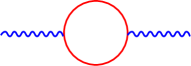
FIG. 1.: Self energy of the $R_{\mu}$ field.

There is no quartic coupling in ${\cal L}_{2}(\pi)$, so only the diagram of fig. [1] contributes; the curly external lines denote $R_{\mu}$’s, the internal solid lines $\pi$’s. The overall factor of $N$ in $\Pi^{\mu\nu}(P)$ arises because each vertex involves a $SU(N)$ commutator, and so, in component notation, is proportional to the structure constant $f^{abc}$; thus fig. [1] is proportional to $f^{acd}f^{bcd}=N\delta^{ab}$. For arbitrary $P$ the complete integral in $\Pi^{\mu\nu}(P)$ is involved, but when $K$ is hard and $P$ soft, in the numerator of the integral we can neglect the terms $\sim K^{\mu}P^{\nu}$, $P^{\mu}K^{\nu}$, and $P^{\mu}P^{\nu}$ relative to that $\sim K^{\mu}K^{\nu}$. For this remaining integral we then isolate the term $\sim T^{2}$, which defines the hard thermal loop [4]:

$$T\sum_{n}\!\!\int\!\!\frac{d^{3}k}{(2\pi)^{3}}\frac{K^{\mu}K^{\nu}}{K^{2}(K+P)^{2}}\approx\frac{T^{2}}{24}(\delta^{\mu\nu}\!-\!\delta\Pi^{\mu\nu}(P)).$$ (11)

In an effective lagrangian, the term $\sim\delta^{\mu\nu}$ changes the coefficient of $tr(R_{\mu}^{2})$ from $f_{\pi}^{2}$ to $f^{2}_{\pi}(T)$ in (2). There are several equivalent ways of writing the effective lagrangian for hard thermal loops [4]-[6]; instead of following the original form of Taylor and Wong[5], we include $\delta\Pi^{\mu\nu}$, and go from momentum to coordinate space, by using[6]

$$T\sum_{m}\int\frac{d^{3}p}{(2\pi)^{3}}\;tr\left(R_{\mu}\;\delta\Pi^{\mu\nu}(P)\;R_{\nu}\right)=$$ (12)

$$\int\!\!d^{4}x\!\!\int\!\!\frac{d\Omega_{\hat{k}}}{4\pi}\,tr\!\!\left(\!\!(\partial_{\mu}R_{\alpha}\!\!-\!\!\partial_{\alpha}R_{\mu})\frac{\hat{K}^{\alpha}\hat{K}^{\beta}}{-(\partial\cdot\hat{K})^{2}}(\partial_{\mu}R_{\beta}\!\!-\!\!\partial_{\beta}R_{\mu})\!\!\right),$$

$\partial\cdot\hat{K}=\partial_{\mu}\hat{K}^{\mu}$. We introduce a four vector $\hat{K}^{\mu}=(i,\hat{k})$, with $\hat{k}$ a three vector of unit norm, $\hat{k}^{2}=1$, so that $\hat{K}^{\mu}$ is null, $\hat{K}^{2}=0$. This is a dummy variable, in that one integrates over all directions of $\hat{k}$, as $\int d\Omega_{\hat{k}}/(4\pi)$.

In (12) $R_{\mu}$ appears as $\partial_{\mu}R_{\alpha}-\partial_{\alpha}R_{\mu}$, etc., because in momentum space $\delta\Pi^{\mu\nu}$ is transverse, $P^{\mu}\delta\Pi^{\mu\nu}(P)=0$. There is another way of seeing why this combination arises. Assume that any hard thermal loop of the $R_{\mu}$’s is of the form $\int d\Omega_{\hat{k}}(\partial_{\alpha}R_{\beta})\hat{K}^{\delta}\hat{K}^{\gamma}/(\partial\cdot\hat{K})^{2}(\partial_{\lambda}R_{\kappa})$, and consider contracting the six indices in all possible ways. Using the equation of motion $\partial_{\mu}R_{\mu}=0$, and the identity $\int d\Omega_{\hat{k}}/(\partial\cdot\hat{K})^{2}=4\pi/\partial^{2}$ [6], one can show that all possible contractions reduce either to $tr(R_{\mu}^{2})$ or to (12).

In (11) we compute the hard thermal loop in the self energy of $R_{\mu}$, but there are also hard thermal loops between three or any higher number of $R_{\mu}$’s. In a gauge theory, because the cubic vertex can bring in a factor of the hard loop momentum, while the quartic vertex is independent of momentum, the diagrams which contribute to hard thermal loops with three or more gauge fields include only cubic, and never quartic, vertices [4]. To sum up all such diagrams, as in fig. [2], we can then neglect the second term in ${\cal L}_{2}(\pi)$, and consider $\pi$ as a matter field in interaction with a background gauge field $R_{\mu}$. Once we are dealing with a gauge theory, however, the general form of the effective lagrangian is uniquely determined by invoking gauge invariance, in this instance for an adjoint field with coupling constant $=\frac{1}{2}$. To make (12) gauge invariant we merely replace $\partial\cdot\hat{K}$ by $D\cdot\hat{K}$, and, because of (9), $\partial_{\mu}R_{\nu}-\partial_{\nu}R_{\mu}$ by $2F_{\mu\nu}$. Hence to leading order in an expansion about zero temperature and momentum, $\sim(T^{2}/f_{\pi}^{2})P^{2}$, the dominant corrections to the chiral lagrangian are given by $\delta{\cal L}_{2}$ [9],

$${\cal L}_{2}+\delta{\cal L}_{2}=-\frac{f^{2}_{\pi}(T)}{4}\;tr(R_{\mu}^{2})$$ (13)

$$-\frac{NT^{2}}{12}\int\frac{d\Omega_{\hat{k}}}{4\pi}\;tr\left(F_{\mu\alpha}\frac{\hat{K}^{\alpha}\hat{K}^{\beta}}{-(D\cdot\hat{K})^{2}}F_{\mu\beta}\right)\;.$$

If we naively power count momenta, then $R_{\mu}\sim P_{\mu}$ and $F_{\mu\nu}\sim P_{\mu}P_{\nu}$. This shows that the reason why we can get a new term of the same order as ${\cal L}_{2}\sim P^{2}$ is because $\delta{\cal L}_{2}$ is nonlocal, $\int F(1/\partial^{2})F\sim P^{2}(1/P^{2})P^{2}\sim P^{2}$.

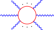
FIG. 2.: Diagrams which contribute to $\delta{\cal L}_{2}$.

The nonlocal term in $\delta{\cal L}_{2}$ only matters for scattering processes where $\partial_{0}g\neq 0$. In the static limit, $\partial_{0}g=0$, the nonlocal term in $\delta{\cal L}_{2}\sim R_{0}^{2}$ [6]. For static chiral fields $R_{0}=0$, and so ${\cal L}_{2}+\delta{\cal L}_{2}$ reduces to $-f_{\pi}^{2}(T)tr(R_{i}^{2})/4$. Expanding $\delta{\cal L}_{2}$ in terms of pion fields, $g=exp(i\pi/f_{\pi})$, to lowest order $R_{\mu}\sim i\partial_{\mu}\pi/f_{\pi}$ and $F_{\mu\nu}\sim[\partial_{\mu}\pi,\partial_{\nu}\pi]/f_{\pi}^{2}$. Thus the nonlocal term in $\delta{\cal L}_{2}$ first appears in scattering processes involving four or more pions.

While the formal analogy between chiral and gauge fields is very useful, the physics which follows is rather different. The original lagrangian of the chiral field, $\sim tr(R_{\mu}^{2})$, is for the gauge field a gauge variant mass term, and so doesn’t arise. Gauge fields have a hard thermal loop in their self energy, which generates the screening of electric and (time dependent) magnetic fields. For chiral fields, the nonlocal term in $\delta{\cal L}_{2}$ doesn’t affect the propagation of pions, only their scattering. Lastly, in gauge theories hard thermal loops are, for soft momenta, as large as the terms at tree level; consequently, a consistent perturbative expansion requires their resummation through an effective expansion. For soft, cool pions, on the other hand, the hard thermal loops are just corrections $\sim T^{2}/f_{\pi}^{2}$, and except for exceptional circumstances, do not dominate the terms at tree level.

To illustrate such an exception, consider the elastic scattering between two pions, of different isospin, in the forward direction. Sitting in the center of mass frame of the two incident pions, with euclidean conventions the momenta for the process $1^{a}2^{b}\rightarrow 3^{c}4^{d}$ are $P_{1}=(ip,\vec{p})=-P_{3}$ and $P_{2}=(ip,-\vec{p})=-P_{4}$; the superscripts denote the isospin indices, $a=c\neq b=d$. The original lagrangian ${\cal L}_{2}$ generates four pion scattering amplitudes $\sim P^{2}/f_{\pi}^{2}$, with hard thermal loops from $\delta{\cal L}_{2}$ down by $T^{2}/f_{\pi}^{2}$. For this special choice of momenta and isospin, however, the term from ${\cal L}_{2}$, $=\delta^{ac}\delta^{bd}(P_{1}+P_{3})^{2}/f_{\pi}^{2}$, vanishes, and the leading term is from $\delta{\cal L}_{2}$, $=\frac{2}{9}\delta^{ac}\delta^{bd}(T^{2}/f_{\pi}^{2})(p^{2}/f_{\pi}^{2})$. In this way, hard thermal loops generate novel scattering amplitudes between Goldstone bosons at nonzero temperature; perhaps this might be observable in spin waves.

We can also use these techniques to compute the leading corrections at low temperature to anomalous processes. Purely hadronic anomalous processes are only allowed when $N\geq 3$, and are described by the Wess-Zumino-Witten term[2]. This can be written as a lagrangian in five dimensions,

$${\cal L}_{5}=\frac{iN_{c}}{240\pi^{2}}\;\epsilon^{\alpha\beta\delta\gamma\kappa}\;tr(R_{\alpha}R_{\beta}R_{\delta}R_{\gamma}R_{\kappa})\;,$$ (14)

where $N_{c}$ is the number of colors, $N_{c}=3$ in $QCD$, and $\epsilon^{\alpha\beta\delta\gamma\kappa}$ is the completely antisymmetric tensor. Up to an overall integer $=N_{c}$, the coefficient of ${\cal L}_{5}$ is determined by topology in five dimensions [2]. At the quark level, ${\cal L}_{5}$ arises from diagrams related to the quark anomaly. In terms of the chiral fields, we call a term anomalous if it is odd under the transformation of $g\rightarrow g^{\dagger}$; such terms have abnormal intrinsic parity [2]. The original ${\cal L}_{2}$ is not anomalous, ${\cal L}_{5}$ is.

After the redefinition of $g$ in (3), and using the complete equations of motion including ${\cal L}_{5}$, $\int d^{5}x{\cal L}_{5}\rightarrow\int d^{5}x{\cal L}_{5}+\int d^{4}x{\cal L}_{5}(\pi)$, where ${\cal L}_{5}(\pi)$ is a lagrangian density in four dimensions,

$${\cal L}_{5}(\pi)=\frac{iN_{c}}{24\pi^{2}f_{\pi}^{2}}\epsilon^{\alpha\beta\delta\gamma}\;tr\left(\partial_{\alpha}\pi\{\left[\pi,R_{\beta}\right],R_{\delta}R_{\gamma}\}\right),$$ (15)

and $\{\cdot,\cdot\}$ denotes the anticommutator. We then compute the anomalous diagram between four $R_{\mu}$’s at one loop order, using ${\cal L}_{5}(\pi)$ at one vertex and ${\cal L}_{2}(\pi)$ at the other.

Once the commutator and anticommutator in the vertex of (15) are contracted with the $f^{abc}$ from the commutator of (7), the matrix structure simplifies significantly. It is natural to introduce another kind of vector potential, $A_{\mu}$, and a field strength, $G_{\mu\alpha}$,

$$A_{\mu}=\epsilon^{\mu\beta\delta\gamma}\;R_{\beta}R_{\delta}R_{\gamma}\;\;\;,\;\;\;G_{\mu\alpha}=\partial_{\mu}A_{\alpha}-\partial_{\alpha}A_{\mu}\;.$$ (16)

Unlike $R_{\mu}$, $A_{\mu}$ is neither a pure gauge transformation, nor does it transform as a gauge field under $SU(N)$ gauge transformations. We introduce the abelian part of the field strength for $A_{\mu}$, $G_{\mu\alpha}$, because of (12).

The integral which arises is again $\Pi^{\mu\nu}(P)$. Keeping only the terms $\sim T^{2}$, as $tr(A_{\mu}R_{\mu})=0$, the term $\sim\delta^{\mu\nu}$ in (11) doesn’t contribute to the anomalous amplitude between four $R_{\mu}$’s, while that $\sim\delta\Pi^{\mu\nu}$ does. Following (13), we then generalize this amplitude between four $R_{\mu}$’s to write the dominant corrections to the anomalous effective lagrangian as $\delta{\cal L}_{5}$,

$$\delta{\cal L}_{5}=-\frac{iN_{c}T^{2}}{144\pi^{2}f_{\pi}^{2}}\int\frac{d\Omega_{\hat{k}}}{4\pi}\;tr\left(\!G_{\mu\alpha}\frac{\hat{K}^{\alpha}\hat{K}^{\beta}}{-(D\cdot\hat{K})^{2}}F_{\mu\beta}\!\!\right).$$ (17)

Even though $G_{\mu\alpha}$ does not transform covariantly under $SU(N)$ gauge transformations, since the leading anomalous terms are given by a single insertion of $G_{\mu\alpha}$, we can still use the $SU(N)$ gauge invariance to sum all one loop diagrams with one insertion of ${\cal L}_{5}(\pi)$, and any number of cubic vertices from ${\cal L}_{2}(\pi)$, by replacing $\partial\cdot\hat{K}$ with $D\cdot\hat{K}$, and $\partial_{\mu}R_{\beta}-\partial_{\beta}R_{\mu}$ with $2F_{\mu\beta}$, in (17).

Expanding in terms of pion fluctuations, as before the field strength $F_{\mu\nu}$ is quadratic in the $\pi$’s, while $G_{\mu\nu}\sim\partial_{[\mu,}\epsilon_{\nu]\alpha\beta\delta}\partial^{\alpha}\pi\partial^{\beta}\pi\partial^{\delta}\pi/f_{\pi}^{3}$ is cubic. Thus both ${\cal L}_{5}$ and $\delta{\cal L}_{5}$ contribute to a five-point interaction, $KK\rightarrow\pi\pi\pi$ [2]. Counting powers of momenta, $\delta{\cal L}_{5}\sim P^{4}(1/P^{2})P^{2}\sim P^{4}$ is of the same order as $\int dx_{5}{\cal L}_{5}\sim P^{4}$.

Although $\delta{\cal L}_{2}$ alters the coefficient of $tr(R_{\mu}^{2})$ in ${\cal L}_{2}+\delta{\cal L}_{2}$, $\delta{\cal L}_{5}$ doesn’t affect that of ${\cal L}_{5}$. Since the normalization of ${\cal L}_{5}$ is fixed by topology in five dimensions, this is natural; the fluctuations, like ${\cal L}_{5}(\pi)$, are always four dimensional, and so only produce corrections in four dimensions, such as $\delta{\cal L}_{5}$. The same thing happens at zero temperature[8].

This approach can also be used to compute the temperature corrections to the chiral lagrangian including the coupling to external gauge fields[10]. This exercise is interesting in its own right; for example, we find that the amplitude for $\pi^{0}\rightarrow 2\gamma$ decreases to $\sim T^{2}/f_{\pi}^{2}$. This is in accord with the behavior near the chiral phase transition, where this amplitude vanishes [11].

To conclude, cool pions give us a broader perspective on hard thermal loops. For example, at next to leading order about zero temperature, $\sim T^{4}/f_{\pi}^{4}$, besides corrections to the nonlocal terms in $\delta{\cal L}_{2}$ and $\delta{\cal L}_{5}$, perhaps there are also new, nonlocal terms. This suggests that the known hard thermal loops, as discussed herein, are themselves the first terms in an infinite series of nonlocal effective lagrangians at nonzero temperature.

This work is supported by a DOE grant at Brookhaven National Laboratory, DE-AC02-76CH00016.

REFERENCES

• [1] S. Weinberg, Physica 96A, 327 (1979); J. Gasser and H. Leutwyler, Ann. of Phys. 158, 142 (1984); J. F. Donoghue, E. Golowich, and B. R. Holstein, Dynamics of the Standard Model (Cambridge Univ. Press, NY, 1992); G. Ecker, Prog. Part. Nucl. Phys. 35, 1 (1995).
• [2] J. Wess and B. Zumino, Phys. Lett 37B, 95 (1971); E. Witten, Nucl. Phys B223, 422 (1983).
• [3] P. Binetruy and M. K. Gaillard, Phys. Rev. D32, 931 (1985); J. Gasser and H. Leutwyler, Phys. Lett. 184B, 83 (1987); M. Dey, V. L. Eletsky, and B. L. Ioffe, ibid. 252B, 620 (1990); A. Bochkarev and J. Kapusta, Phys. Rev. D54, 4066 (1996); R. D. Pisarski and M. Tytgat, ibid. D54, 2989 (1996).
• [4] R. D. Pisarski, Phys. Rev. Lett. 63, 1129 (1989); E. Braaten and R. D. Pisarski, Nucl. Phys. B337, 569 (1990); ibid. B339, 310 (1990); J. Frenkel and J. C. Taylor, ibid. B334, 199 (1990); ibid. B374, 156 (1992); J. P. Blaizot and E. Iancu, ibid. B390, 589 (1993); ibid. B417, 608 (1994); ibid. B434, 662 (1995); R. Efraty and V. P. Nair, Phys. Rev. D47, 5601 (1993); R. Jackiw and V. P. Nair, ibid. D48, 4991 (1993); R. Jackiw, Q. Liu, and C. Lucchesi, ibid. D49, 6787 (1994); P. F. Kelly, Q. Liu, C. Lecchesi, and C. Manuel, ibid. D50, 4209 (1994).
• [5] J. C. Taylor and S. M. H. Wong, Nucl. Phys. B346, 115 (1990).
• [6] E. Braaten and R. D. Pisarski, Phys. Rev. D45, 1827 (1992).
• [7] A. M. Polyakov, Gauge fields and strings, (Harwood Press, London, 1987).
• [8] J. F. Donoghue and D. Wyler, Nucl. Phys. B316, 289 (1989); R. Akhoury and A. Alfakih, Ann. Phys. 210, 81 (1991); J. Bijnens, Nucl. Phys. B367, 709 (1991).
• [9] If instead of (3) we define $g\rightarrow u(exp(i\pi/f_{\pi}))u$ and expand about a background field $u$, then the covariant derivative which appears in the ensuing ${\cal L}_{2}(\pi)$ is $D_{\mu}=\partial_{\mu}+\frac{1}{2}[V_{\mu},\cdot]$, where VΞΌ=uβ€ β€‹βˆ‚ΞΌu+uβ€‹βˆ‚ΞΌu†subscriptπ‘‰πœ‡superscript𝑒†subscriptπœ‡π‘’π‘’subscriptπœ‡superscript𝑒†V_{\mu}=u^{\dagger}\partial_{\mu}u+u\partial_{\mu}u^{\dagger}. Viewed as an $SU(N)$ gauge field, $V_{\mu}$ is not a pure gauge transformation, and so the field strength $F_{\mu\nu}=\partial_{\mu}V_{\nu}-\partial_{\nu}V_{\mu}+\frac{1}{2}[V_{\mu},V_{\nu}]$ is nontrivial. With this parametrization, the effective lagrangian ${\cal L}_{2}+\delta{\cal L}_{2}$ of (13) is given by taking $R_{\mu}=(u^{\dagger})^{2}\partial_{\mu}u^{2}$ in $tr(R_{\mu}^{2})$, and this $D_{\mu}$ and $F_{\mu\nu}$ in the nonlocal term. While this form of the effective lagrangian appears very different, on the mass shell it should give the same scattering amplitudes as (13).
• [10] R. D. Pisarski and M. Tytgat, manuscript in preparation.
• [11] R. D. Pisarski, Phys. Rev. Lett. 76, 3084 (1996).