[

.

Weakly first-order phase transitions: the $\epsilon$ expansion vs. numerical simulations
in the cubic anisotropy model

Abstract

Some phase transitions of cosmological interest may be weakly first-order and cannot be analyzed by a simple perturbative expansion around mean field theory. We propose a simple two-scalar model—the cubic anisotropy model—as a foil for theoretical techniques to study such transitions, and we review its similarities and dissimilarities to the electroweak phase transition in the early universe. We present numerical Monte Carlo results for various discontinuities across very weakly first-order transitions in this model and, as an example, compare them to $\epsilon$-expansion results. For this purpose, we have computed through next-to-next-to-leading order in $\epsilon$.

]

Renormalization-group (RG) techniques for studying phase transitions, such as the $\epsilon$ expansion, have been used for over twenty years, and the analysis of second-order transitions has produced quite successful quantitative predictions [1, 2, 3]. Weakly first-order transitions, in which the transition dynamics is dominated by long but finite wavelength fluctuations, were also investigated using $\epsilon$ expansion techniques [4, 5, 6]. However, there has been less emphasis on testing quantitative predictions for such first-order transitions, in part because few predictions were easily accessible to experiments of the time [7].

In recent years, renewed interest in quantitative predictions for weakly first-order transitions has arisen in cosmology, specifically the genesis of matter. Current electroweak theory holds the promise of explaining the net baryon number of the universe [8]. Any scenario of baryogenesis must satisfy Sakharov’s conditions of (i) baryon number violation, (ii) C and CP violation, and (iii) departure from thermal equilibrium. Electroweak theory has all of these ingredients: baryon number violation comes from a quantum anomaly, C and CP violation is built in, and a first-order electroweak phase transition can provide the departure from equilibrium. The electroweak transition separates the low-temperature world, where the SU(2)$\times$U(1) gauge symmetry is hidden and only the U(1) symmetry of electromagnetism is manifest, from the high-temperature domain where the full SU(2)$\times$U(1) symmetry is manifest. To test the viability of electroweak baryogenesis, detailed understanding of many properties of this phase transition is required.

FIG. 1.: Phase diagram of electroweak theory, or the cubic anisotropy model (for $u\leq 0,v\geq 0$), based purely on analytic arguments. The left and right axes show the relevant ratio $R$ of couplings for electroweak theory, or for the cubic anisotropy model, respectively.

Fig. 1 sketches what can be firmly established about the phase diagram of electroweak theory in the minimal Standard Model (the standard model with a single SU(2) doublet Higgs field) without resorting to numerical simulations. A more complicated Higgs sector is probably needed for realistic electroweak baryogenesis, but the minimal case is easier to discuss and provides a useful testing ground. The one important parameter of the minimal model not well determined by experiment is the Higgs boson mass $m_{\rm h}$, or equivalently, the Higgs quartic self-coupling $\lambda$. For a sufficiently light Higgs mass (or small $\lambda$) the phase transition can be successfully treated by expanding around mean field theory and is known to be fluctuation-induced first order. In other words, it appears to be second-order in mean field theory, but perturbative fluctuations generate a finite correlation length and render the transition first order. For large Higgs mass (or large $\lambda$), the problem becomes difficult to analyze. Perturbative techniques are only reliable when $m_{\rm h}{\ll}M_{\rm W}$, where $M_{\rm W}\approx 80$ GeV is the W-boson mass. In condensed matter applications, this is commonly referred to as the Ginsburg criteria for the success of mean field theory. An equivalent way of stating this criteria is that the ratio of couplings $R\equiv\lambda/g_{\rm w}^{2}$, where $g_{\rm w}^{2}$ is the electroweak gauge coupling, needs to be small. If one (unrealistically) sends $g_{\rm w}$ (and hence $M_{\rm W}$) to zero, so as to probe the opposite $R\to\infty$ extreme, there is one piece of solid information. The Higgs sector decouples from the gauge interactions in this limit, and becomes a pure O(4) symmetric scalar theory, which is known to have a second-order transition.

Viable electroweak baryogenesis generally needs as strong a first-order phase transition as possible, and so prefers as small a Higgs mass as possible. Experiment, however, puts lower bounds on Higgs masses (60 GeV in the minimal model) and forces one into the regime where a perturbative analysis of the transition is at best marginal. Consequently, there is a need to understand the full phase diagram for electroweak theory and to develop techniques for reliable computations even when $m_{\rm h}\gtrsim M_{\rm W}$.

There are several things known about the transition in various unphysical limits. Near but just below 4 spatial dimensions ($d{=}4-\epsilon$), the transition remains first order for large Higgs mass [9, 10], as we review below. In the large $N$(scalar) limit (or in $2+\epsilon$ dimensions), there is a value of $m_{\rm h}$ at which there is a tricritical point, and the transition becomes second-order for larger $m_{\rm h}$ [10, 11]. In contrast, recent lattice simulations suggest that the first-order line actually ends in a critical point at $m_{\rm h}\approx M_{\rm W}$, above which there is no phase transition whatsoever [12]. There has been a recent attempt to understand this behavior using RG methods in three dimensions [13].

In all the cases outlined above, one is left with the problem of how to analyze the phase transition for those Higgs masses where it is only weakly first-order and where perturbation theory breaks down. For any techniques that purport to address this problem, it would be useful to have an extremely simple statistical system—on the level of simplicity of the Ising model—that could serve as a canonical initial testing ground. The Ising model provides a canonical example of a second-order transition and is in the same universality class as the continuum field theory of a single scalar field. To study weak first-order transitions, one may add a second spin field to make a model known as the Ashkin-Teller model, or equivalently add a second scalar field to make a model known as the cubic anisotropy model.

The purpose of the present work is to review these models; review the similarities and dissimilarities with the electroweak phase transition (see also [14]); present the results of numerical simulations of first-order transitions; and, as an example of testing a theoretical method, compare the numerical results to predictions of the $\epsilon$ expansion. The $\epsilon$ expansion is the generalization of a theory from three to $4{-}\epsilon$ spatial dimensions, where the dynamics of long wavelength fluctuations is tractable using RG-improved perturbation theory, followed by extrapolation of results back to $\epsilon{=}1$. We have studied weakly first-order transitions of the cubic anisotropy model through next-to-next-to-leading order in $\epsilon$. (Leading order results were obtained twenty years ago in ref. [4].) We propose the cubic anisotropy model as a benchmark for other investigators who advocate particular techniques for studying weakly first-order transitions. The details of our $\epsilon$ expansion calculations and numerical studies are given elsewhere [15, 16].

In its general form, the cubic anisotropy model is an O($n$) symmetric scalar model to which an additional interaction is added which breaks O($n$) down to hyper-cubic symmetry [3]:

$$S=\!\int\!d^{d}x\left({1\over 2}\left|\partial\vec{\phi}\right|^{2}+{t\over 2}\left|\vec{\phi}\right|^{2}+{u\over 4!}\left|\vec{\phi}\right|^{4}+{v\over 4!}\sum_{i=1}^{n}\phi_{i}^{4}\right)\!.$$ (1)

We shall focus on the simplest case, $n{=}2$. This model is analogous to electroweak theory when $u\leq 0$ and $v\geq 0$. Fig. 1 illustrates the phase structure for weak couplings ($|u|,v\ll 1$). There is again a suitable ratio of couplings,

$$R\equiv(v-n|u|)/|u|\,,$$ (2)

which defines a Ginsburg criteria. When the ratio drops below zero, the tree-level potential in (1) is unstable, just as $\lambda<0$ makes the Higgs potential unstable in electroweak theory. When the ratio is small, perturbation theory turns out to be well behaved. Then the phase transition is first order and, like electroweak theory, is fluctuation driven. When the ratio is moderate or large, perturbation theory breaks down. When it is infinite, corresponding to $u{=}0$, the theory reduces to $n$ decoupled copies of a theory of a single scalar field. Each such copy is in the same universality class as the Ising model, and has a second-order transition.

To further appreciate the similarities between the cubic anisotropy model and the electroweak phase transition, we turn to the $\epsilon$ expansion. When $\epsilon$ is small, both theories can be solved using RG-improved perturbation theory. Fig. 2a depicts the RG flow of the couplings $g_{\rm w}$ and $\lambda$ of electroweak theory in $4{-}\epsilon$ spatial dimensions as one examines increasingly large distance scales. Not shown is the third relevant parameter, the running Higgs mass, which always grows (relative to the renormalization point) as one scales to larger distances. For $g_{\rm w}{\not=}0$, the couplings do not flow to any fixed point. They do, however, flow into the region $\lambda\ll g_{\rm w}^{2}$, where the Ginsburg criteria is satisfied. After using the renormalization group to flow into this region, one can use standard perturbative techniques to make quantitative computations of thermal properties and conclude that the transition is first order. This is the argument that, for sufficiently small $\epsilon$, the line of first order transitions shown in Fig. 1 continues all the way to $R=\infty$.

In condensed matter physics, the underlying theory at short distances is typically strongly interacting. In contrast, the Higgs model in particle physics is generally of interest as a fundamentally weakly coupled ($\lambda,g_{\rm w}\ll 1$) theory at short distances [17]. Hence, one can focus attention on short-distance theories defined by varying $\lambda/g_{\rm w}^{2}$ in the neighborhood of the Gaussian fixed point at $\lambda{=}g_{\rm w}{=}0$, as illustrated by the arc $A$ near the origin in Fig. 2a. By renormalization group equivalence, this covers all theories in the lightly shaded region of fig. 2a. In particular, it covers the case of the real world ($g_{\rm w}$ fixed but $\lambda$ unknown, designated by line $B$), provided the Higgs mass is not so large that the scalar sector is fundamentally non-perturbative (i.e., $m_{\rm h}\lesssim$ 1 TeV).

Analogous flows for the cubic anisotropy model are show in fig. 2b. For $u\leq 0$ and $v\geq 0$, the flows are qualitatively similar to the electroweak case. For $u=0$, the theory flows to the Ising fixed point. For $u$ small and negative, it instead flows to a region where the Ginsburg criteria is met and the transition is known to be first order—an observation first exploited by Rudnick [4]. The Ising fixed point is a tricritical point separating first-order ($u<0$) and second-order ($u>0$) transitions.

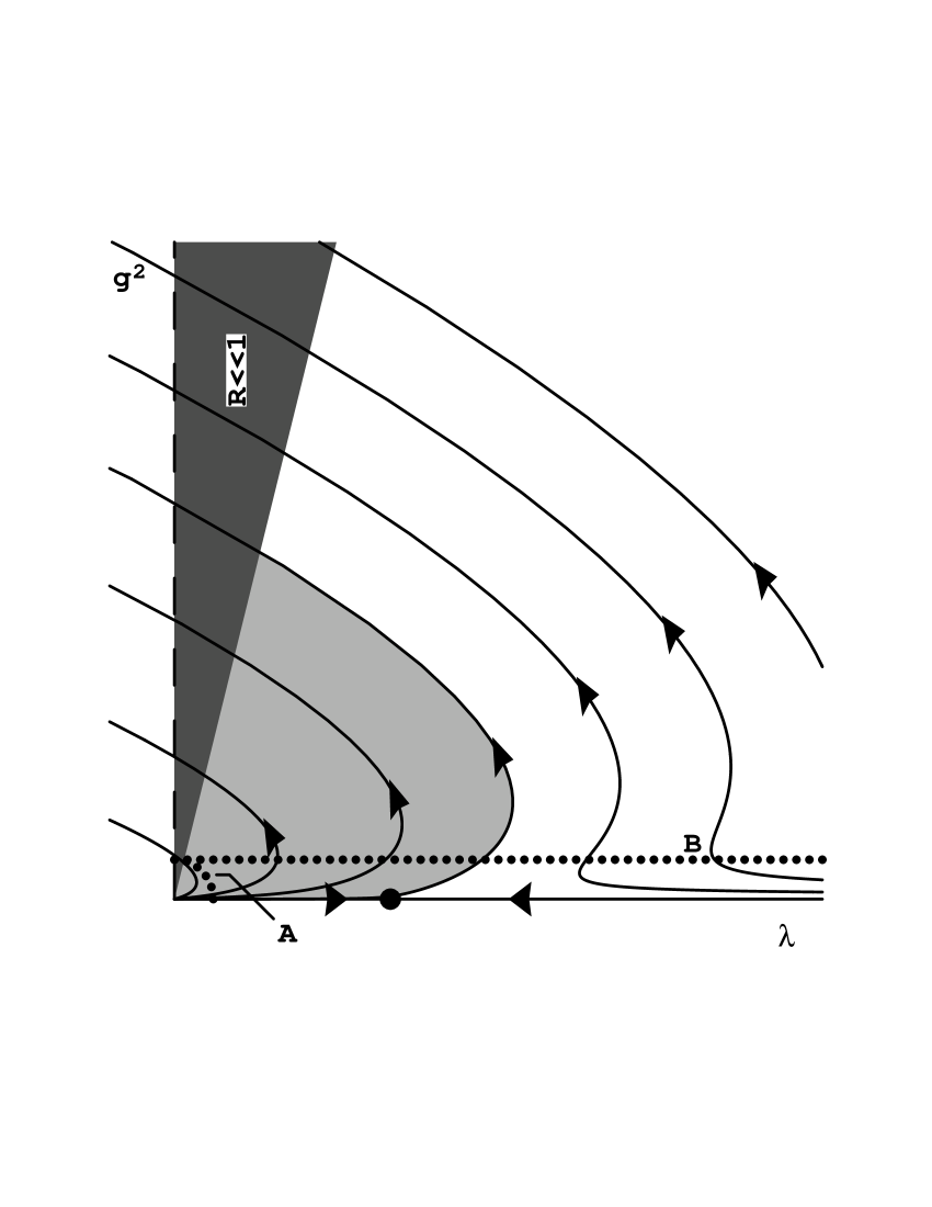
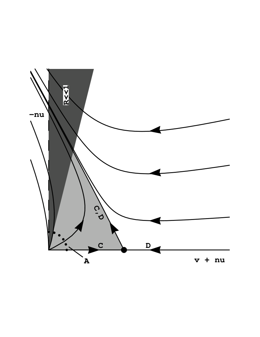
FIG. 2.: Renormalization group flows, for small $\epsilon$, of (a) electroweak theory, and (b) the cubic anisotropy model.

An important distinction between the cubic anisotropy model and electroweak theory is that the cubic anisotropy model must have a phase transition for any choice of the Ginsburg ratio $R$ because a global symmetry is spontaneously broken. No such argument holds for electroweak theory due to Elitzur’s theorem [18].

In analogy with electroweak theory, one could attempt to analyze the phase transitions in the cubic anisotropy model for weak couplings $u$ and $v$, and for arbitrary choices of the Ginsburg ratio $R$. However, we know that the transition gets weaker, and the analysis will become harder, as $R$ increases. So an instructive goal is to analyze the extreme case $R\to\infty$. The limiting renormalization group trajectory is the one marked $C$ in Fig. 2b that runs from the Gaussian fixed point to the Ising fixed point, and then away from the Ising fixed point to the perturbative regime. This extreme case has a substantial advantage for numerical simulations: the same long-distance theory in the perturbative regime can be reached starting from a strongly coupled short-distance theory described by the trajectory $D$ which comes in from ($u{=}0,v{=}\infty$) to the Ising fixed point and then flows away to the perturbative regime along $C$. The advantage of starting with this strongly coupled theory is that it can be replaced by a discrete spin model, which is easier to simulate numerically than theories with continuous-valued fields.

In the (lattice regularized) theory of a single scalar field with

$$S=\int d^{d}x\>\left[{\textstyle{1\over 2}}(\partial\phi)^{2}+\lambda(\phi^{2}-v^{2})^{2}\right]\,,$$ (3)

the field $\phi$ is constrained to only take on the two values $\pm v$ when $\lambda\to\infty$, and hence the theory reduces to a simple Ising model with a discrete two component spin. Similarly, the strong coupling limit of the $n=2$ cubic anisotropy model is a model of two coupled Ising spins $s$ and $t$ known as the Ashkin-Teller model [19, 20]:

$$S=-\beta\sum_{\langle ij\rangle}(s_{i}s_{j}+t_{i}t_{j}+x\,s_{i}s_{j}t_{i}t_{j})\,,$$ (4)

where the sum is over all neighboring pairs of sites $(i,j)$; the spins $s,t={\pm}1$; and $\beta$ and $x$ are parameters that represent the inverse temperature and the deviation from the limit of decoupled Ising models, respectively. The $R\to\infty$ limit in our discussion of the cubic anisotropy model corresponds to the $x{\to}0^{+}$ limit of the Ashkin-Teller model.

The $x{\to}0^{+}$ limit is crucial if one wants the Ashkin-Teller model to correspond to the continuum cubic anisotropy model. That is because generic first-order transitions have finite correlation lengths of $O(1)$ lattice spacings at the transition. Everything about such transitions depends on the details of the short-distance physics: the type of lattice used, the exact details of the couplings, etc. In the $x{\to}0^{+}$ limit, however, the correlation length at the transition becomes arbitrarily large (since for $x=0$ it is infinite), and so in this limit the details of the short-distance physics decouple. Dimensionful quantities like the correlation length $\xi$ aren’t directly useful quantities to predict in this limit, since they diverge, but ratios such as

$$\lim_{x\to 0^{+}}\>{\xi_{+}\over\xi_{-}}\equiv\lim_{x\to 0^{+}}\>{\lim_{\beta\to\beta^{-}}\>\xi\over\lim_{\beta\to\beta^{+}}\>\xi}$$ (5)

are non-trivial and universal. Here $\xi_{+}$ is the correlation length infinitesimally above the critical temperature, and $\xi_{-}$ is that infinitesimally below. Our project has been to compute such ratios in the $\epsilon$ expansion for the cubic anisotropy model and to compare to numerical simulations of the corresponding Ashkin-Teller model.

The details of our $\epsilon$ expansion calculations are given in ref. [15]. We find

$${\chi_{+}\over\chi_{-}} = 2\,\bigl{[}1+\epsilon\,(-0.1063\ln\epsilon+0.4494)$$ (6)

$$+ \epsilon^{2}(-0.0073\ln^{2}\epsilon+0.1647\ln\epsilon-0.2859)+O(\epsilon^{3})\bigr{]},$$ (7)

$${\xi_{+}^{2}\over\xi_{-}^{2}} = 2\,\bigl{[}1+\epsilon\,(-0.1063\ln\epsilon+0.4139)+O(\epsilon^{2})\bigr{]},$$ (8)

$${C_{+}\over C_{-}} = \textstyle{17\over 320}\,[\,\epsilon+\epsilon^{2}(-0.2125\ln\epsilon+1.3993)+O(\epsilon^{3})].$$ (9)

$C$ is the specific heat. $\chi\equiv\partial\langle\phi_{1}\rangle/\partial h|_{h=0}$ is the scalar susceptibility, defined by adding an interaction $h\phi_{1}$ to the model, and to leading order is the same as $\xi^{2}$. Our leading-order results for the $\chi$ and $C$ ratios differ by factors of 4 from those originally reported by Rudnick [4].

Table I summarizes the leading-order and next-to-leading order results for our three ratios. In general, $\epsilon$ expansions are asymptotic expansions and the coefficients begin to grow after just a few terms. For critical exponents, one can often get reasonably good values by simply adding terms at $\epsilon{=}1$ until the contributions start to increase. Our results in the cubic anisotropy model are not as well-behaved as the best Ising model series, but are comparable to the $\epsilon$ expansion for the exponent $\eta$. The expansion for $\chi_{+}/\chi_{-}$ leads one to expect that the actual result should lie somewhere between the LO and NLO results. One might have a similar expectation for $C_{+}/C_{-}$ and $\xi_{+}/\xi_{-}$, even though the expansion for the former is clearly poorly behaved.

Very accurate predictions for critical exponents in the Ising model have been obtained using resummation techniques which combine knowledge of the asymptotic large order behavior of the series with explicit low-order coefficients [2]. Our series expansions, however, contain logarithms of $\epsilon$, and we do not currently know how to derive the large-order behavior of these series. As explained in ref. [15], these logarithms arise because physics at the phase transition involves two scales whose ratio is $O(\epsilon)$.

Our numerical results are also presented in Table I, and details may be found in ref. [16]. One sees that $C_{+}/C_{-}$ is indeed bracketed by the LO and NLO $\epsilon$-expansion results and that $\xi_{+}/\xi_{-}$ works reasonably well. $\chi_{+}/\chi_{-}$, however, is a disappointment for the $\epsilon$ expansion, since the numerical result is not bracketed by LO and NLO, and the the NNLO correction only makes the agreement worse.

Our results highlight the utility of the cubic anisotropy and Ashkin-Teller models as foils for theoretical methods for making quantitative predictions of weakly first-order transitions. It would be interesting to see the comparison of our numerical results against methods other than the $\epsilon$ expansion, and it would be useful to have more accurate Monte Carlo determinations of the universal ratios.

universal ratio	$\epsilon$ expansion			Monte Carlo
	LO	NLO	NNLO
$C_{+}/C_{-}$	0.053	0.127		0.069(8)
$\xi_{+}/\xi_{-}$	1.4	1.7		1.7(2)
$\chi_{+}/\chi_{-}$	2.0	2.9	2.3	4.1(5)(a)

TABLE I.: Leading (LO), next-to-leading (NLO), and next-to-next-to-leading order (NNLO) results in the $\epsilon$ expansion compared to numerical Monte Carlo results. ^(a) The error estimate on the Monte Carlo measurement of $\chi_{+}/\chi_{-}$ should be taken with a grain of salt (see ref. [16] for details).

This work was supported by the U.S. Department of Energy grants DE-FG06-91ER40614 and DE-FG03-96ER40956.

REFERENCES

- [1] K. Wilson and J. Kogut, Phys. Reports 12, 75–200 (1974), and references therein.
- [2] J. Le Guillou, J. Zinn-Justin, Phys. Rev. Lett. 39, 95 (1977); ibid., J. Phys. (Paris) Lett. 46, L137 (1985); 48, 19 (1987); 50, 1365 (1989); B. Nickel, Physica A 177, 189 (1991).
- [3] For a review, see D. Amit, Field Theory, the Renormalization Group, and Critical Phenomena, revised second edition (World Scientific: Singapore, 1984).
- [4] J. Rudnick, Phys. Rev. B 11, 3397 (1975).
- [5] E. Domany, D. Mukamel, and M. Fisher, Phys. Rev. B 15, 5432 (1975).
- [6] J. Chen, T. Lubensky, and D. Nelson, Phys. Rev. B 17, 4274 (1978).
- [7] We refer not to tricritical scaling exponents, which have been studied in detail, but to things like amplitude ratios which depend on dynamics away from any fixed point.
- [8] For a review, see A. Cohen, D. Kaplan and A. Nelson, Annu. Rev. Nucl. Part. Sci. 43, 27 (1988).
- [9] P. Ginsparg, Nucl. Phys. B170 [FS1], 388 (1980).
- [10] P. Arnold and L. Yaffe, Phys. Rev. D 49, 3003 (1994); Univ. of Washington preprint UW/PT-96-28 (errata).
- [11] J. March-Russel, Phys. Lett. B296, 364 (1992).
- [12] K. Kajantie, M. Laine, K. Rummukainen, and M. Shaposhnikov, Phys. Rev. Lett. 77, 2887 (1996).
- [13] N. Tetradis, CERN report CERN-TH/96-190.
- [14] M. Alford and J. March-Russel, Nucl. Phys. B417, 527 (1994).
- [15] P. Arnold and L. Yaffe, University of Washington report UW/PT-96-23, hep-ph/9610447; P. Arnold and Y. Zhang, UW/PT-96-24, hep-ph/9610448.
- [16] P. Arnold and Y. Zhang, University of Washington report UW/PT-96-26, hep-lat/9610032.
- [17] For our purposes, the scale set by the inverse temperature defines short distance; the so-called “triviality” problem for continuum scalar theories is not relevant.
- [18] S. Elitzur, Phys. Rev. D12, 3978 (1975).
- [19] J. Ashkin and E. Teller, Phys. Rev. 64, 178 (1943).
- [20] R. Ditzian, J. Banavar, G. Grest, and L. Kadanoff, Phys. Rev. B 22, 252 (1980).