Strange Baryonic Matter from Chiral Effective Lagrangians

Abstract

We investigate the existence of bound states of baryons in a kaon condensate using chiral mean field theory. The interactions are described by an effective $\rm{SU(3)}_{L}\!\!\times\!\rm{SU(3)}_{R}$ chiral lagrangian where terms of higher order in density, baryon momentum, and kaon mass are suppressed by powers of the symmetry breaking scale, $\Lambda$. We take up to next to leading order terms ($n=2,3,4$). We search for infinite baryon number solutions, namely “strange baryonic matter”, using a Thomas-Fermi approximation for a slowly varying condensate and a lowest order Hartree approximation to describe the many body interactions. For simplicity we study a pure $K^{0}$ condensate and only neutrons, the lightest baryons in that condensate. We find solutions with neutron number densities, $\rho_{n}\>\raisebox{-3.44444pt}{$\stackrel{{\scriptstyle\textstyle{>}}}{{\sim}}$}\>3.5\rho_{0}$, where $\rho_{0}$ is the infinite nuclear matter density. This is consistent with the estimate of the onset of a K-condensate at $\rho_{n}\simeq$ 2–4 $\rho_{0}$. We show that the binding energies, $E_{b}$, grow with $\rho_{n}$ and for $\rho_{n}<7\rho_{0}$ (at $\rho_{n}\>\raisebox{-3.44444pt}{$\stackrel{{\scriptstyle\textstyle{>}}}{{\sim}}$}\>7\rho_{0}$ perturbative expansion is lost) we find $E_{b}<150MeV$ ($E_{b}<70MeV$ for $\rho_{n}<5\rho_{0}$) even in the most favorable cases. These binding energies may be too low for this type of matter to appear and persist in the early universe.

hep-ph/9610496

UCLA/96/TEP/25

October, 1996

1. Introduction

QCD is the theory of strong interactions among quarks and gluons, the elementary particles that constitute hadrons. With three massless quarks, $m_{u}=m_{d}=m_{s}=0$, the QCD lagrangian has a global chiral $\rm{SU(3)}_{L}\!\!\times\!\rm{SU(3)}_{R}$symmetry. This is considered to be an accidental symmetry, since there is no deeper reason for the (almost) masslessness of these three quarks. The chiral symmetry is approximate since the three quarks masses are small, but not zero. The symmetry is most explicitly violated by the s-quark mass, $m_{s}\simeq 240MeV$, which is much larger than the u and d masses ($m_{u}\simeq 6~{}MeV,m_{d}\simeq 12~{}MeV$). Even if we can not derive from QCD the properties of the quark and gluon bound states, the hadrons, we know the mass spectrum and low momentum interactions of hadrons show the persistence of the $\rm{SU(3)}_{L}\!\!\times\!\rm{SU(3)}_{R}$chiral symmetry. The $SU(3)_{V}$ vectorial and $SU(3)_{A}$ axial vector symmetry groups (those whose generators are the sum and the difference respectively of the left and right generators) are realized differently. The vectorial subgroup $SU(3)_{V}$ is realized in the Wigner–Weyl mode, yielding (almost) degenerate multiplets (octets and tenplets) of baryons and mesons. This is the (approximate) symmetry used to classify hadrons (in the “eightfold way”), that lead to the proposal of quarks as a means to populate the fundamental representation of the group. The axial symmetry $SU(3)_{A}$ is instead realized in the Nambu–Goldstone mode, namely it is spontaneously broken at a scale $\Lambda\simeq 1GeV$ yielding an octet of (quasi) Goldstone bosons, one for each broken generator, the pions, kaons, and eta mesons. The lightness of these mesons compared to the other hadrons justifies this identification. The mass of the Goldstone bosons is a result of the explicit breaking of $SU(3)_{A}$ due to the non-zero quark masses. In fact from the lowest order ($n=2$, see below) chiral lagrangian, the $\pi$, $K$, and $\eta$ masses result linearly proportional to the $u$,$d$, and $s$ quark masses. At this order one gets the phenomenologically successful Gell-Mann Okubo relation among meson masses. This is evidence that the perturbative expansion in the chiral lagrangian is good, namely that higher order terms (that modify the Gell-Mann Okubo relation) are small.

A non–linear effective chiral lagrangian [1] is the most general lagrangian for the baryons and the octet of quasi Goldstone bosons (therefore valid at energies below the scale of spontaneous chiral symmetry breaking, i.e. $E<\Lambda$) which is compatible with the approximate accidental $\rm{SU(3)}_{L}\!\!\times\!\rm{SU(3)}_{R}$chiral symmetry of QCD [2, 3]. Although there are different ways of parametrizing the Goldstone bosons, it has been shown that they all lead to the same observables [4]. This effective non-renormalizable lagrangian consists of a power series expansion in derivatives, baryon fields and the chiral symmetry quark mass matrix ${\cal M}=diag(m_{u},m_{d},m_{s})$. As a trick [2] to use chiral symmetry to also fix the form of the explicit symmetry breaking terms using our knowledge of QCD, the matrix ${\cal M}$ is promoted to a field with its chiral transformation chosen so that it would fix the form of the ${\cal M}$ dependent terms in the QCD lagrangian (if chiral symmetry were exact). The chiral symmetry breaking terms in the effective lagrangian lead to s–wave interactions of the Goldstone mesons, that are very important in the phenomenon of kaon condensation [5, 6]. Without explicit breaking the Goldstone bosons have only derivative couplings, which can be understood by recalling that the Goldstone fields are the angular coordinates that parametrize the orbits of degenerate vacua, so that a change in value of the field can not affect the energy.

A chiral effective lagrangian includes all the terms compatible with the approximate chiral symmetry of QCD with coefficients to be determined phenomenologically when possible. Terms with dimension larger than four have dimensionful parameters which are proportional to, either, inverse powers of the symmetry breaking scale, $\Lambda\simeq 1GeV$, or inverse powers of $f_{\pi}$ as shown in Eq.(2.1) below. This prescription insures that loop corrections to each term generate terms of the same form, if $\Lambda\simeq 4\pi f_{\pi}$ [2, 3]. The usefulness of the expansion resides in the ability of cutting the series after a few terms. Assuming that the expansion parameters (which are, $\partial_{\mu}/\Lambda$, $m_{s}/\Lambda$, and $\rho_{B}/f_{\pi}^{2}\Lambda=\rho_{B}/7\rho_{0}$, see below) are small, the terms in the lagrangian can be organized in successively less important sets and a finite number of terms can be used.

This method provides the only systematic way to implement the symmetries of QCD in $\pi$–$K$–$\eta$–baryon interactions. This method has proven to be useful, in many applications, among which describing properties of bulk hadronic matter, such as the formation of a kaon condensate [5, 6, 7]. It has been shown that due to the kaon’s dominant s-wave coupling to baryons [6] the formation of a kaon condensate is quite insensitive to nuclear interactions. It is believed that a kaon condensate will most likely form at a baryonic density anywhere from 2–4 times nuclear density.

In this paper we are not interested in the details of the onset of the condensation but rather in solutions to the non-linear classical field equations that describe an isolated system consisting of baryons in a K-condensate. In order to approach such a complicated problem many approximations have to be made. The result is a system of equations that resembles those of a liquid droplet [8, 9], where the baryons are treated as a gas of pseudo particles trapped in the bose condensate of kaons [10]. Lynn, Nelson, and Tetradis [10] (LNT from now on) studied this problem using a phenomenological combination of a chiral lagrangian, having no terms with four or more baryon fields and no terms which are higher order than linear in quark masses, and the Walecka lagrangian. The Walecka model [11] consists of two fictitious massive vector and scalar fields, $V^{\mu}$ and $\phi$, coupled to protons and neutrons in a renormalizable lagrangian. It describes well the properties of bulk nuclear matter. LNT added the Walecka lagrangian to incorporate nuclear forces not included otherwise in their model. They also coupled the $\phi$ field to the mesons. Here we only use the chiral effective lagrangian with the four baryon terms and next to leading order terms as well, that include more than four baryons and higher powers of the quark masses. In fact we have shown elsewhere [13] that the four-fermion terms incorporate into the chiral lagrangian the same description of bulk nuclear matter contained in the Walecka model, when baryons are restricted to the nucleon doublet. Because the solutions we find have large densities, we need not only investigate baryon-meson and baryon-baryon interactions but also three baryon interactions (ie. terms with six fermion fields). We are guided here by the belief in a perturbative series dictated by the broken chiral symmetry as explained above where the lowest order terms are dominant. We think that this is the essential difference between our work and LNT’s treatment of the same problem, namely we rely on a perturbative expansion as described above and, as we argue towards the end of this paper in section 8, we believe they do not.

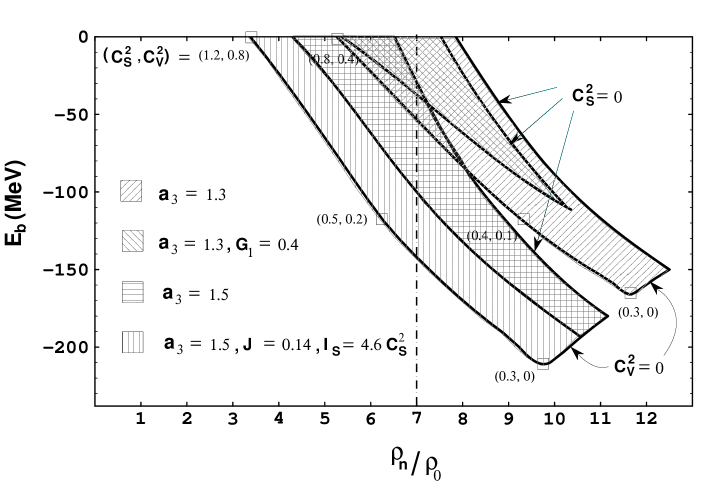
Figure 3: Here we show the regions of physical solutions in ($E_{b}$, $\rho_{n}$) space corresponding to the indicated parameters. We indicate only the values of $a_{3}$ and the higher order parameters taken to be non-zero. We then find the values of $C^{2}_{S}$ and $C^{2}_{V}$ at the left and right boundaries of each band with the procedure described in the text. $C^{2}_{S}$ and $C^{2}_{V}$ are maximum at the left boundaries and $C^{2}_{S}=0$ at the right ones. The lower boundary corresponds to $C^{2}_{V}=0$. The values of ($C^{2}_{S}$,$C^{2}_{V}$) are shown at some points. We have chosen the most favorable values of $a_{3}$ and the higher order parameters to obtain the lowest baryonic number densities $\rho_{n}$ for infinite solutions with a given binding energy $E_{b}$, using a chiral effective lagrangian. Actually only the region of $\rho_{n}<7\rho_{0}$ is consistent with our approach (the perturbative expansion is lost at higher densities), so the rest of the figure may be indicative but is not believable.

This paper is organized as follows. The $\rm{SU(3)}_{L}\!\!\times\!\rm{SU(3)}_{R}$chiral lagrangian we use is presented in section 2 and the necessary approximations and our ansatz are given in section 3. The following four sections discuss the solutions. In section 4 the general method to obtain solutions is explained using just the lowest order lagrangian. Section 5 shows how the requirement of a continuous density allows us to constrain the solutions to bands in binding energy-density space (shown in Fig.3), with just the lowest $n=2$ lagrangian. In section 6 and 7 we add higher order terms one at a time to see if those terms help to obtain solutions with a lower density for a given binding energy. Section 7 contains our main results. In section 8 we compare our work with LNT and section 9 contains our conclusions.

2. The Lagrangian

A term in the Lagrangian consistent with näive dimensional analysis [3] is given by

$$\rm{C}f_{\pi}^{2}\Lambda^{2}\left[{\bar{B}\Gamma_{\alpha}B\over f_{\pi}^{2}\Lambda}\right]^{a}\left[{\overline{\Pi}\over f_{\pi}}\right]^{b}\left[{\partial_{\mu}\over\Lambda}\right]^{c}\left[{\mbox{m}\over\Lambda}\right]^{d}$$ (2.1)

where $f_{\pi}=93\rm{MeV}$, $m=(m_{K},m_{B})$ and at first order in $m_{s}$ $m_{K}^{2}=\Lambda m_{s}$, $m_{s}=240MeV$, we take $m_{u}=m_{d}=0$, and $\Gamma_{\alpha}$ represents 1, $\gamma_{5}$, $\gamma^{\mu}$, $\gamma^{\mu}\gamma_{5}$, and $\sigma^{\mu\nu}$, either multiplied by the $SU_{V}(3)$ generators, $T_{a}$, or not. The order of the terms is given by the index $a+c+d=n$. Terms with $n=2$ are unsupressed. Higher orders are suppressed by $\Lambda^{2-n}$.

The meson matrix $\overline{\Pi}$ is defined as $\Pi_{a}T_{a}$ where $\Pi_{a}$ is the meson octet of Goldstone bosons, and $T_{a}\equiv\lambda_{a}/2$, where $\lambda_{a}$ are the eight Gell-Mann matrices,

$$\overline{\Pi}={1\over\sqrt{2}}\left(\begin{array}[]{ccc}\mbox{${\pi^{0}\over\sqrt{2}}+{\eta\over\sqrt{6}}$}&\pi^{+}&K^{+}\\ \pi^{-}&-{\pi^{0}\over\sqrt{2}}+{\eta\over\sqrt{6}}&K^{0}\\ K^{-}&\overline{K}^{0}&-2{\eta\over\sqrt{6}}\end{array}\right).$$ (2.5)

The baryon octet $B_{a}$ also appears in the combination $B=B_{a}T_{a}$,

$$B=\left(\begin{array}[]{ccc}{\Sigma^{0}\over\sqrt{2}}+{\Lambda\over\sqrt{6}}&\Sigma^{+}&p\\ \Sigma^{-}&{-\Sigma^{0}\over\sqrt{2}}+{\Lambda\over\sqrt{6}}&n\\ \Xi^{-}&\Xi^{0}&-2{\Lambda\over\sqrt{6}}\end{array}\right).$$ (2.9)

We consider only the octet of baryons because they are the lightest of the baryon multiplets. Finally, $\rm{C}$ in Eq.(2.1) is a coefficient of O(1). Notice that powers of the meson field, $\overline{\Pi}$, are not suppressed by powers of $\Lambda$, since it appears in the combination $\overline{\Pi}/f_{\pi}$. The derivative factor operates on both meson and baryon fields. For the baryon fields, however, only the spatial derivatives should be included. We are not using a heavy baryon formalism here since the effective mass of the baryons will be small compared to their momentum (see the examples provided by the values of $m^{*}$ in the Table 1). Since we are using a Hartree approximation, where the baryons are treated as free pseudo particles, we can use the equation of motion to replace time derivatives by spatial derivatives in the interaction lagrangian [12]. Notice that the density, $\rho=\bar{B}\gamma_{0}B$, appears in the expansion parameter, $\rho/f_{\pi}^{2}\Lambda\simeq\rho/7\rho_{0}$ where $\rho_{0}$ is nuclear density, $\rho=1.28~{}10^{6}MeV^{3}$. Therefore, in order to keep the chiral expansion reliable we need solutions with densities $\rho<7\rho_{0}$ and we do not expect them at $\rho$ below the onset of $K$ condensation estimated at $2$–$4\rho_{0}$. Thus we work in the region in which the perturbative expansion in baryonic density is marginal. With $\rho=3.4\rho_{0}$ the expansion term $\bar{B}\Gamma_{\alpha}B/{f_{\pi}^{2}\Lambda}$ is of the same order of magnitude as ${m_{K}/\Lambda}$.

We choose the terms in our lagrangian which satisfy the condition $a+c+d=2,3$.

$${\cal{L}}_{chiral} = {1\over 4}f_{\pi}^{2}Tr\partial_{\mu}\Sigma\partial^{\mu}\Sigma^{\dagger}+{1\over 2}f_{\pi}^{2}\Lambda Tr[{\cal M}\Sigma+h.c.]$$ (2.10)

$$\mbox{}+Tr\bar{B}(i\partial/-m_{B})B+iTr\bar{B}\gamma^{\mu}[{\cal{V}}_{\mu},B]$$

$$\mbox{}+DTr\bar{B}\gamma^{\mu}\gamma_{5}\{{\cal{A}}_{\mu},B\}+FTr\bar{B}\gamma^{\mu}\gamma_{5}[{\cal{A}}_{\mu},B]$$

$$\mbox{}-a_{1}Tr\bar{B}(\xi{\cal M}\xi+h.c.)B-a_{2}Tr\bar{B}B(\xi{\cal M}\xi+h.c.)$$

$$\mbox{}-a_{3}Tr[{\cal M}\Sigma+h.c.]Tr\bar{B}B+{C_{\alpha}\over f_{\pi}^{2}}Tr\bar{B}\Gamma_{\alpha}B\bar{B}\Gamma^{\alpha}B$$

$$\mbox{}+{G_{\alpha}\over f_{\pi}^{4}\Lambda}Tr\bar{B}B\bar{B}\Gamma_{\alpha}B\bar{B}\Gamma^{\alpha}B+{H_{\alpha}\over f_{\pi}^{2}\Lambda}Tr[\bar{B}\Gamma_{\alpha}\partial/B\bar{B}\Gamma^{\alpha}B+h.c.]$$

$$\mbox{}+\cdots$$

where the dots indicate terms of higher order and a few of the same order, which involve different ways of contracting the baryon octet that within our approximations give no new terms later. The non-linear sigma field, $\Sigma$, is given by

$$\Sigma=\exp{(2i\overline{\Pi}/f_{\pi})}$$ (2.11)

and the field, $\xi$, is defined as

$$\xi\equiv\sqrt{\Sigma}=\exp{(i\overline{\Pi}/f_{\pi})}.$$ (2.12)

The explicit symmetry breaking is expressed as an expansion in powers of the small quark mass $m_{s}$, an element of the quark mass matrix $\cal M$,

$${\cal M}=\left(\begin{array}[]{ccc}0&&\\ &0&\\ &&m_{s}\end{array}\right).$$ (2.16)

Finally, we have the meson vector and axial vector currents

$$\cal{V}_{\mu} = {1\over 2}(\xi^{\dagger}\partial_{\mu}\xi+\xi\partial_{\mu}\xi^{\dagger})$$

$$\cal{A}_{\mu} = {i\over 2}(\xi^{\dagger}\partial_{\mu}\xi-\xi\partial_{\mu}\xi^{\dagger}).$$ (2.17)

Most of the coefficients in Eq.(2.10) are fixed by low energy NN and $\pi N$ scattering, and by mass splittings in the baryon octet. Their tree level values are

$$\begin{array}[]{rclrclrcl}D&=&0.81,&F&=&0.44,&&&\\ a_{1}&=&0.28,&a_{2}&=&-0.56,&a_{3}&=&1.3\pm 0.2,\\ m_{s}&=&240\rm{MeV},&m_{B}&=&584\rm{MeV},&\Lambda&\simeq&1\rm{GeV}\end{array}$$ (2.18)

and, $C_{\alpha}$, $G_{\alpha}$, and $H_{\alpha}$ are free parameters of $O(1)$.

3. Ansatz and Approximations

We choose a simplifying ansatz [10] with only one non-vanishing meson expectation value, $\langle K^{0}\rangle$. In the presence of this VEV the baryon masses are modified with the lightest baryon being the neutron. For simplicity we will study the formation of bound states with only neutrons. We hope that this can be instructive in searching for solutions with more degrees of freedom. Our ansatz for the classical meson expectation value is, therefore,

$$\overline{\Pi}={1\over\sqrt{2}}\left(\begin{array}[]{ccc}0&0&0\\ 0&0&\langle K^{0}\rangle\\ 0&\langle\overline{K}^{0}\rangle&0\end{array}\right)$$ (3.1)

where $\langle K^{0}\rangle$ is chosen to be real, and from the hermiticity of $\overline{\Pi}$ we get ${\langle\overline{K}^{0}\rangle=\langle K^{0}\rangle}$.

We are interested in finding classical solutions of the equations of motion consisting of bound states at zero pressure and with large baryon number. In order to minimize their surface energy these solution should be spherically symmetric. Furthermore, we will consider bound states large enough for the surface effects to be negligible. We take the density of baryons and the value of the meson field to be almost constant throughout the interior. Using the Thomas-Fermi approximation [14] we assume that the kaon fields vary slowly compared to the baryon wavelength, i.e. $\vec{\nabla}K^{0}/f_{\pi}\ll\vec{k}$, where $\vec{k}$ is the neutron’s wavenumber. This allows us to effectively treat the neutrons at each point as a Fermi gas in a constant kaon field. Finally, since the kaon field is slowly varying we find that all p-wave and higher derivative interactions are negligible compared to s-wave interactions. With the ansatz given in Eq.(3.1), the vector current, $\mathcal{V}_{\mu}$, vanishes and the terms with axial vector coupling—$D$ and $F$ terms—to the neutrons given in Eq.(2.10) also vanish. With these simplifications the lagrangian reduces to

$${\cal{L}}_{chiral} = {1\over 2}f_{\pi}^{2}\partial_{\mu}\theta\partial^{\mu}\theta-f_{\pi}^{2}m_{K}^{2}(1-\cos{\theta})$$ (3.2)

$$\,+\bar{n}(i\partial/-m_{n}^{*})n-{C_{V}^{2}\over 2f_{\pi}^{2}}n^{\dagger}nn^{\dagger}n$$

$$\,+{C_{S}^{2}\over 2f_{\pi}^{2}}\bar{n}n\bar{n}n+{G_{1}\over 3f_{\pi}^{4}\Lambda}\bar{n}n\bar{n}n\bar{n}n$$

$$\,+{G_{2}\over f_{\pi}^{4}\Lambda}n^{\dagger}nn^{\dagger}n\bar{n}n+{H_{1}\over f_{\pi}^{2}\Lambda}\bar{n}i\vec{\gamma}\cdot\vec{\nabla}n\bar{n}n$$

where $\theta={\sqrt{2}\langle K^{0}\rangle/f_{\pi}}$, we have used the first order (in $m_{s}$) relation $m_{K}^{2}=m_{s}\Lambda$, $n$ is the neutron field, $m_{n}^{*}$ is the neutron mass within the $\langle K^{0}\rangle$ condensate [10],

$$m_{n}^{*}=m_{N}-a_{t}m_{s}(1-\cos{\theta}),$$ (3.3)

with $a_{t}=2a_{3}+a_{2}+a_{1}=2.32\pm 0.4$ and $m_{N}$ the free neutron mass, $m_{N}=939MeV$. Notice that a constant has been added to the lagrangian in Eq.(3.2) so that the $\theta$ dependence of ${\cal{L}}_{chiral}$ disappears from the lagrangian when $\theta=0$. This is the origin of the $(1-\cos{\theta})$ factor in the second term of ${\cal{L}}_{chiral}$ in Eq.(3.2). Notice that there is also a factor $(1-\cos{\theta})$ in $m_{n}^{*}$, Eq.(3.3), so that $m_{N}$ is the physical neutron mass (outside the condensate). The constant $m_{N}$ contains, therefore, all contributions of the form $Tr\bar{B}B$ in Eq.(2.10) obtained by setting $\xi=1$ and $\Sigma=1$, thus $m_{N}=m_{B}+2m_{s}(a_{3}+a_{2})$ (actually, knowing $a_{2}$ and $a_{3}$ this relation fixes $m_{B}$, Eq.(2.18)).

The three vector momentum and spin dependent terms containing currents of the form $\bar{n}\gamma^{i}n$ and $\bar{n}\gamma^{i}\gamma_{5}n$, where $i$ are the spatial degrees of freedom, average to zero in spherically symmetric bulk matter. Furthermore, all terms containing time derivatives of the condensate vanish as a result of minimizing the thermodynamical potential at fixed electric charge: the time dependence turns out to be simple harmonic with the frequency equal to the electric charge [5, 6].

4. Infinite Solutions with Lowest Order $\mathbf{n=2}$ Terms

Let us first analyze the $n=2$ terms of Eq.(3.2) ($G_{1}=G_{2}=H_{1}=0$). The Thomas-Fermi approximation allows one to take a free particle wave function, $\!\exp{i(\vec{k}\cdot\vec{x}-\epsilon_{k}t)}$, for the neutron, where $\vec{k}$ and $\epsilon_{k}$ are the space dependent wavenumber and energy respectively. The Dirac equation for a neutron moving in the mean field of all other neutrons is

$$\left[i\partial/-m_{n}^{*}-{C_{V}^{2}\over f_{\pi}^{2}}(n^{\dagger}n)\gamma^{0}+{C_{S}^{2}\over f_{\pi}^{2}}(\bar{n}n)\right]n=0,$$ (4.1)

and by substituting in the neutron wave function, we get

$$\left[\gamma^{0}(\epsilon_{k}-{C_{V}^{2}\over f_{\pi}^{2}}(n^{\dagger}n))-\gamma^{i}k_{i}-(m_{n}^{*}-{C_{S}^{2}\over f_{\pi}^{2}}(\bar{n}n))\right]n=0.$$ (4.2)

Squaring the above equation and applying Dirac algebra we get the dispersion relation of a free quasi-particle,

$$\epsilon^{*2}-k^{2}-m^{*2}=0,$$ (4.3)

where we define the effective energy and mass of the quasi-particle to be

$$\epsilon^{*} \equiv \epsilon_{k}-{C_{V}^{2}\over f_{\pi}^{2}}n^{\dagger}n$$ (4.4)

$$m^{*} \equiv m_{n}^{*}-{C_{S}^{2}\over f_{\pi}^{2}}\bar{n}n.$$ (4.5)

The zero temperature ground state, $|\Psi\rangle$, of our system can be found by minimizing the thermodynamic potential, $\Omega$. For fixed baryon number, $B$,

$$\Omega=E_{total}-\mu_{B}B,$$ (4.6)

where $\mu_{B}$ is the baryon chemical potential and $B=\int d^{3}xn^{\dagger}n$. The total energy of the system, $E_{total}$, is given by

$$E_{total}=T^{00}=\int d^{3}x(\varepsilon_{k}+\varepsilon_{n}+{\cal U}_{\theta})$$ (4.7)

where $\varepsilon_{k}$ is the kinetic energy density of the condensate,

$$\varepsilon_{k}={1\over 2}{f_{\pi}}^{2}({\dot{\theta}}^{2}+(\vec{\nabla}\theta)^{2})\\ ={1\over 2}f_{\pi}^{2}(\vec{\nabla}\theta)^{2},$$

$\varepsilon_{n}$ is the neutron energy density,

$$\varepsilon_{n}=2\int^{k_{f}}{{d^{3}k\over(2\pi)^{3}}(k^{2}+m^{*2})^{{1\over 2}}}+{C_{V}^{2}\over 2f_{\pi}^{2}}(n^{\dagger}n)^{2}+{C_{S}^{2}\over 2f_{\pi}^{2}}(\bar{n}n)^{2},$$ (4.8)

and ${\cal U}_{\theta}$ is the potential energy density of the condensate

$${\cal U}_{\theta}=f_{\pi}^{2}m_{K}^{2}(1-\cos{\theta}).$$ (4.9)

The thermodynamic potential, $\Omega$, is a function of the Fermi momentum, $k_{f}$, the $\langle K^{0}\rangle$ condensate, $\theta$, and $\mu_{B}$ as well as the other coefficients in the Lagrangian. First we functionally minimize $\Omega$ with respect to $k_{f}(\vec{x})$, and find

$$\mu_{B}=\mu^{*}+{C_{V}^{2}\over f_{\pi}^{2}}n^{\dagger}n,$$ (4.10)

where $\mu^{*}$ is the quasi-particle’s chemical potential defined as the value of $\epsilon^{*}$ at $k=k_{f}$. Eq.(4.10) is equivalent to Eq.(4.4) with $k=k_{f}$, hence, $\mu_{B}$ is equivalent to the energy of a neutron at the top of the Fermi sea, which is therefore constant over all space. Different choices for the chemical potential lead to different sizes of finite solutions, i.e. to different numbers of neutrons within it.

Functionally minimizing $\Omega$ with respect to $\theta(\vec{x})$ results in a differential equation for the condensate, $\theta$,

$$\vec{\nabla}^{2}(f_{\pi}\theta)-{\partial\over\partial(f_{\pi}\theta)}\left[P_{n}-{\cal U}_{\theta}\right]=0,$$ (4.11)

where $P_{n}$, the pressure of the neutron gas, is given by

$$P_{n} = \mu_{B}n^{\dagger}n-\varepsilon_{n}$$ (4.12)

$$= {1\over 3}T^{ii}=(\bar{n}\vec{\gamma}\cdot\vec{k}n)+{C_{V}^{2}\over 2f_{\pi}^{2}}(n^{\dagger}n)^{2}-{C_{S}^{2}\over 2f_{\pi}^{2}}(\bar{n}n)^{2}.$$ (4.13)

In the zero temperature ground state the neutron number density is

$$\rho_{n}=\langle\Psi|n^{\dagger}n|\Psi\rangle=2\int^{k_{f}}{d^{3}k\over(2\pi)^{3}}={k_{f}^{3}\over 3\pi^{2}},$$ (4.14)

the scalar density

$$\rho_{S} = \langle\Psi|\bar{n}n|\Psi\rangle=2\int^{k_{f}}{d^{3}k\over(2\pi)^{3}}{m^{*}\over\sqrt{k^{2}+m^{*2}}}$$ (4.15)

$$= {m^{*}\over 2\pi^{2}}\left[k_{f}\mu_{B}-{{m^{*}}^{2}\over 2}\ln{\left({\mu_{B}+k_{f}\over\mu_{B}-k_{f}}\right)}\right],$$

and

$$\langle\Psi|(\bar{n}\vec{\gamma}\cdot\vec{k}n)|\Psi\rangle = 2\int^{k_{f}}{{d^{3}k\over(2\pi)^{3}}{k^{2}\over\sqrt{k^{2}+m^{*2}}}}$$ (4.16)

$$= {3\over 4\pi^{2}}\left[\mu_{B}\left({k_{f}^{3}\over 3}-{k_{f}{m^{*}}^{2}\over 2}\right)+{{m^{*}}^{4}\over 4}\ln{\left({\mu_{B}+k_{f}\over\mu_{B}-k_{f}}\right)}\right].$$

Substituting Eqs.(4.5), (4.10), (4.14), and (4.15) into the equation for the dispersion relation at the top of the Fermi sea,

$${\mu^{*}}^{2}-k_{f}^{2}={m^{*}}^{2}$$ (4.17)

we get a a transcendental equation of the variables $k_{f}$ and $\theta$ which we solve numerically to get $k_{f}(\theta)$. We can now solve Eq.(4.11) after plugging $k_{f}(\theta)$ into Eq.(4.13) to obtain $P_{n}(\theta)$ .

We can view Eq.(4.11) as a one dimensional newtonian equation of motion [9] for a particle of unit mass moving in a potential, $V_{\mathit{eff}}$, with the following replacements:

$$f_{\pi}\theta\rightarrow x,\hskip 28.45274ptr\rightarrow t,\hskip 28.45274pt\left[P_{n}-{\cal U}_{\theta}\right]\rightarrow V_{\mathit{eff}}(x).$$ (4.18)

Writing Eq.(4.11) in radial coordinates, we get (for our spherically symmetrical, time independent condensate $\theta$)

$${d^{2}(f_{\pi}\theta)\over dr^{2}}+{2d(f_{\pi}\theta)\over rdr}=-{d(P_{n}-{\cal U}_{\theta})\over d(f_{\pi}\theta)}.$$ (4.19)

Notice that the “damping term” decreases as $1/r$ which means it becomes negligible for large “times” in the newtonian analogy. The potential, $V_{\mathit{eff}}=P_{n}-{\cal U}_{\theta}$ for an infinite baryon solution, with $C_{V}^{2}=.24$, $C_{S}^{2}=.63$, and $\mu_{B}=900\rm{MeV}$, is shown in Fig.1. The potential has two degenerate maxima one at $\theta_{0}=1.37$ and the other at the true vacuum, $\theta=0$. In the newtonian analogy a test particle starts from the top of the hill at $\theta_{0}=1.37$ and waits there for a very long time during which the damping term becomes effectively zero. The particle then accelerates quickly through the valley reaching the top of the other hill, the true vacuum, where it comes to a stop. Therefore, the solutions for a large number of baryons have constant $\theta$ and density over a large volume and a small spherical surface region where one vacuum state evolves rapidly to the other. One can isolate the infinite solutions by imposing the following conditions on $V_{\mathit{eff}}$,

$$V_{\mathit{eff}}(\theta_{0}) = V_{\mathit{eff}}(\theta=0)\,=\,0$$

$$\left.\frac{dV_{\mathit{eff}}(\theta)}{d\theta}\right|_{\theta_{0}} = 0.$$ (4.20)

where $\theta_{0}$ is the value of the condensate at the center of the solution, $r=0$. Notice that for an infinite solution $V_{\mathit{eff}}(\theta_{0})=\mu_{B}n^{\dagger}n-\varepsilon_{n}-{\cal U}_{{\theta}_{0}}=0$ and in the constant interior of the solution $\varepsilon=\varepsilon_{n}+{\cal U}_{{\theta}_{0}}$ giving the relation,

$$\mu_{B}={\varepsilon\over\rho_{n}},$$ (4.21)

thus the energy per neutron is $\mu_{B}$.

The strangeness density of each solution is found as the zero component of the strangeness current, $S_{\mu}=(J_{Y})_{\mu}-(J_{B})_{\mu}$, where $J_{Y}$ is the strong hypercharge current and $J_{B}$ is the baryon number current. With our approximations the only non zero contribution to $S_{0}$ comes from the meson vector current coupling $iTr\bar{B}\gamma^{\mu}[{\cal{V}}_{\mu},B]$ term in Eq.(2.10), and it is $S_{0}=(1-\cos\theta_{0})n^{\dagger}n$ so the strangeness per baryon number of the strange matter is just $(1-\cos\theta_{0})$ (see Table 1).

5. Mapping Out the Solution Space

The model we are considering so far with only $n=2$ terms, which is equivalent to the Walecka model for bulk nucleonic matter [11], has only two parameters, $C_{V}^{2}$ and $C_{S}^{2}$. Notice that the coefficients $C_{S}^{2}$ and $C_{V}^{2}$ are positive definite and the signs of the terms are chosen to account for the scalar attraction and vector repulsion observed in nuclear interactions. Thus we have four unconstrained parameters, $C_{S}^{2}$, $C_{V}^{2}$, $\mu_{B}$, and $\theta_{0}$, and two constraining conditions on $V_{\mathit{eff}}$, Eq.(4. Infinite Solutions with Lowest Order $\mathbf{n=2}$ Terms). We are left with two independent variables that we choose to be $\mu_{B}$ and $C_{S}^{2}$. Since the main properties of the infinite solutions we are looking for are their baryon density, $\rho_{n}$, and their binding energy, $E_{b}$, we will show the regions of solutions in the $(\rho_{n},E_{b})$ space. This is equivalent in the variables we are talking about to a $(\theta_{0},\mu_{B})$ space. This is so because $\rho_{n}=k_{f}^{3}/3{\pi}^{2}$ depends on $\theta_{0}$ through the monotonically increasing (see below) function, $k_{f}(\theta_{0})$, and $E_{b}=\mu_{B}-m_{N}$, see Eq.(4.21), inside the infinite solution, i.e. in bulk baryonic matter. For a given $\mu_{B}$, i.e. a given $E_{b}$, there is a range of allowed number densities, that depend on $C_{V}^{2}$ and $C_{S}^{2}$, $\rho_{n}=\rho_{n}(C_{V}^{2},C_{S}^{2})$, but $C_{V}^{2}$ also depends on $C_{S}^{2}$, $C_{V}^{2}=C_{V}^{2}(C_{S}^{2})$. $C_{V}^{2}$ can be shown numerically to increase monotonically with $C_{S}^{2}$, while $\rho_{n}$ decreases monotonically with $C_{S}^{2}$. So, the allowed range of $\rho_{n}$ for each $E_{b}$ corresponds to an allowed range of $C_{S}^{2}$ values, $0\leq C_{S}^{2}\leq(C_{S}^{2})_{max}$. It turns out $(C_{S}^{2})_{max}$ can be found in a systematic way, that we pass now to explain.

Let us return to Eq.(4.17), the transcendental equation whose roots we solve numerically for to find $k_{f}$ at a fixed $\theta$. Using Eqs.(4.10) and (4.14) we see that $\mu^{*}=\mu_{B}-({C_{V}}^{2}/f_{\pi}^{2})(k_{f}^{3}/3{\pi}^{2})$, therefore the l.h.s. of Eq.(4.17) does not explicitly depend on $\theta$. Through Eqs.(4.5) and (4.15) we see that the r.h.s., ${m^{*}}^{2}$, carries the explicit $\theta$ dependence of Eq.(4.17) through $m_{n}^{*}$. The l.h.s. depends on $\mu_{B}$, $C_{V}^{2}$, and $k_{f}$ and the r.h.s. depends on $C_{S}^{2}$ and $k_{f}$. Figs.2a and 2c are examples of the sides of Eq.(4.17) as functions of $k_{f}$ for particular $C_{S}^{2}$ and $C_{V}^{2}$ values. The l.h.s are shown with black dashed lines for a given $\mu_{B}$ ($\mu_{B}=900MeV)$, the r.h.s. are shown for different $\theta$ values with gray solid lines. The shape of the gray solid curves depends in a complicated way on $C_{S}^{2}$. For each $\theta$, the intersections of the corresponding gray line with the dashed line gives the solution $k_{f}(\theta)$. The dashed line moves up and down the diagram with $\mu_{B}$ without changing shape. For a fixed $\mu_{B}$, as $\theta$ increases from zero the solution $k_{f}(\theta)$ starts departing from zero and grows continuously to a maximum value where all the gray lines turn over, thus $k_{f}(\theta)$ is a monotonically increasing function. This happens when there is only one intersection (for $\mu_{B}$ and $\theta$ fixed). This is the case of Fig.2a. However there are cases, such as the one shown in Fig.2c, in which there are three intersections (see the three x’s). We can see in Fig.2c that as $\theta$ increases (gray line lowers with respect to the dashed line) the first two intersections approach each other, get to coincide at the point where the two intersecting curves have the same slope, and disappear, leaving only the third intersection. If we had taken the $1^{st}$ intersection as the physical $k_{f}(\theta)$, at the $\theta$ value for which the two first intersections disappear, after joining in one point, there would be a discreet jump in $k_{f}$ from this point to the $3^{rd}$ intersection, at a larger value of $k_{f}$, which becomes now the only intersection. This jump in $k_{f}$ is unphysical, since the density $\rho_{n}\sim k_{f}^{3}$ has to be a continuous function of the condensate, $\theta$, as $\theta$ grows from zero outside the bound state to its maximum value in the interior. Thus we impose conditions on the l.h.s. and r.h.s. of Eq.(4.17) as functions of $k_{f}$ to forbid the values of $C_{S}^{2}$ (for each $\mu_{B}$) for which triple intersections appear. These are conditions on the slope of the intersecting curves (i.e. the l.h.s and the r.h.s.) as functions of $k_{f}$. Valid solutions only occur when at $k_{f}=0$ the r.h.s, ${m^{*}}^{2}$ (gray line) is lower than the l.h.s., $({\mu^{*}}^{2}-k_{f}^{2})$ (black dashed line), see Figs.2a and 2c. This insures that as the condensate $\theta$ increases (gray line lowers) $k_{f}(\theta)$ (and the baryon density) increases smoothly from zero near the surface of the solution. The curves cross when they intersect and ${m^{*}}^{2}$ becomes larger. If the ${m^{*}}^{2}$ curve is more concave than the $({\mu^{*}}^{2}-k_{f}^{2})$ one, they cross again. This is the case we reject, namely when

$${d\over dk_{f}}\left({m^{*}}^{2}-{\mu^{*}}^{2}+k_{f}^{2}\right)<0.$$ (5.1)

for any value of $\theta$ and $k_{f}$. Notice that both slopes are negative and we reject the case in which the ${m^{*}}^{2}$ slope is larger (more negative) than the other. We show the difference in slope for a rejected case (the one of Fig.2c) in Fig.2d. Fig.2b shows an allowed border line case (the one of Fig.2a) in which the difference in slope would become negative (for some values of $k_{f}$ and $\theta$) if $C_{S}^{2}$ would be increased. This is the important numerical result that allows us to get an upper bound on $C_{S}^{2}$, the fact that the difference in slopes (i.e. the l.h.s. of Eq.(5.1)) decreases with increasing $C_{S}^{2}$. Thus, the border line case for each $\mu_{B}$ fixes $(C_{S}^{2})_{max}$.

Now we can explain the procedure actually followed to map out the solution space. First, we choose a $\mu_{B}$ (or equivalently $E_{b}$). Then vary $C_{V}^{2}$ and $C_{S}^{2}$ and look at $V_{\mathit{eff}}$ (solving Eq.(4.17) to get $k_{f}(\theta))$ until the conditions for an infinite solution, Eq.(4. Infinite Solutions with Lowest Order $\mathbf{n=2}$ Terms), are fulfilled, namely until the maximum of $V_{\mathit{eff}}$ is at zero. This is not difficult to do after noticing that increasing $C_{S}^{2}$ (scalar attraction) raises $V_{\mathit{eff}}$ and increasing $C_{V}^{2}$ (vector repulsion) lowers $V_{\mathit{eff}}$. Once a set $(C_{S}^{2},C_{V}^{2})$ corresponding to an infinite solution has been found, we look at the l.h.s. of Eq.(5.1) (i.e. the difference of the slopes of both sides of Eq.(4.17)). If it corresponds to an allowed case (positive difference in slope) $C_{S}^{2}$ is increased, otherwise $C_{S}^{2}$ is decreased, and the shape of $V_{\mathit{eff}}$ has to be checked again to obtain another $C_{V}^{2}$ so that the new $(C_{S}^{2},C_{V}^{2})$ corresponds to an infinite solution. One keeps doing this until finding an infinite solution corresponding to a border line case (Fig.2b) for the difference in slope. At this point we have found $(C_{S}^{2})_{max}$ for the given $\mu_{B}$, and its corresponding $C_{V}^{2}$ and $\theta_{0}$. This procedure determines the $({\rho_{n}})_{min}$ border of the allowed regions in $(E_{b},\rho_{n})$ space. The $({\rho}_{n})_{max}$ border corresponds to $C_{S}^{2}=0$ and the $C_{V}^{2}$ value necessary to satisfy Eq.(4. Infinite Solutions with Lowest Order $\mathbf{n=2}$ Terms), for each $\mu_{B}$. The allowed regions found are shown in Fig.3 with labels $a_{3}=1.3$ and $a_{3}=1.5$. The parameter $a_{3}$ appears in ${m_{n}}^{*}$, Eq.(3.3). It is measured through the nucleon $\sigma$-term to be $a_{3}=1.3\pm 0.2$. It is the parameter responsible for the s-wave attraction between kaons and nucleons, that yield K-condensation. We see in Fig.3 that a higher value of $a_{3}$, i.e. a lower value of the effective nucleon mass, $m_{n}^{*}$, helps to find solutions at lower densities. Only values of $C_{V}^{2}\geq 0$ are allowed, producing the lower boundaries shown in the figure with the $C_{V}^{2}=0$ label. Some values of $(C_{V}^{2},C_{S}^{2})$ are also shown.

Notice that the procedure we follow is only self consistent for $\rho_{n}/\rho_{0}<7$, since the perturbative expansion in baryon bilinears $\bar{B}\Gamma_{\alpha}B$ is lost at larger densities. The rest of the diagram for $\rho_{n}>7\rho_{0}$ in Fig.3 may be indicative but is not believable. In any case, we were not expecting solutions below the density necessary for the onset of K-condensation, $2$–$4$ $\rho_{0}$. This is consistent with the densities we find, starting at $4.5\rho_{0}$. At these densities, the fermion bilinear expansion parameter $\sim\rho_{n}/7\rho_{0}$ is large and higher order terms with more baryons should be considered.

6. Solutions with Higher Order $\mathbf{n=3}$ Terms

Let us describe the effect of taking into account the $G_{1}$, $G_{2}$, and $H_{1}$ terms in ${\cal L}_{chiral}$, Eq.(3.2). These are the only remaining terms of order $n=3\,(a+c=3)$, besides the $a_{1},a_{2},a_{3}$ terms $(a+d=3)$, already included in our initial lagrangian, because they are the lowest order terms providing an s-wave (i.e. derivative or momentum independent) K-B couplings, thus without them kaons and baryons would not be coupled within bulk baryonic matter.

The procedure we follow to examine the effect of these higher order terms is to add only one term at a time. This increases by one the number of free parameters, $\mu_{B}$, $\theta_{0}$, $C_{V}^{2}$, $C_{S}^{2}$. However we reduce the problem again to just the old four parameters by fixing the new one. We choose both negative and positive values of $O(1)$ for the single higher order parameter studied, within a range that insures the higher order term in the lagrangian is never larger than the $C_{V}^{2}$ and $C_{S}^{2}$ terms. Then we proceed as before choosing a $\mu_{B}$ value and finding $(C_{S}^{2})_{max}$ (and the corresponding $(\rho_{n})_{min}$, etc.) as described above.

We are interested in knowing which higher order terms help to get solutions with lower density $\rho_{n}$ for a given binding energy. The three baryons $G_{1}$ and $G_{2}$ terms raise $(\rho_{n})_{min}$ instead, as well as the $H_{1}$ term with positive $H_{1}$ values, while with negative $H_{1}$ values it can lower $(\rho_{n})_{min}$ although very little. An example of the effect of these terms is shown for $G_{1}=0.4$ (and $a_{3}=1.3$) in Fig.3. The region of allowed solutions in $(\rho_{n},E_{b})$ is a wedge because $(C_{S}^{2})_{max}$ becomes zero at the tip (and the $(\rho_{n})_{max}$ boundary corresponds to $C_{S}^{2}=0$). Other examples with $G_{1}$, $G_{2}$, and $H_{1}$ positive and negative are given in Table 1. This table shows the values of $(C_{S}^{2})$, $(C_{V}^{2})$, the one higher order parameter chosen to be non-zero, the baryon number density, the effective mass $m^{*}$ of the quasi particles and the condensate $\theta_{0}$, for which the baryon number density is minimum (corresponding to the maximum values of $(C_{S}^{2})$ and $(C_{V}^{2})$ for which solutions exist, after fixing the higher order parameter to the largest positive and negative physically acceptable values) for a fixed binding energy $E_{b}=-39MeV$ and parameter $a_{3}=1.3$. While $G_{1}$ does not introduce any major change in the self consistent procedure described above used to find solutions, the $G_{2}$ and $H_{1}$ terms turn the $\mu^{*}$ algebraic Eq.(4.10) into a transcendental equation, (see Eq.(A.1) in the appendix with either $H_{1}=I_{V}=0$ or $G_{2}=I_{V}=0$). The appendix gives the complete equations with all the higher order terms included in this paper for the effective neutron chemical potential, effective neutron mass, pressure and energy density that we label with the sub index “_TOTAL”. Notice that the $H_{1}$ term in Eq.(3.2) contains a derivative of the nucleon field so it modifies the momentum of the neutrons. Adding only $H_{1}$ to the $C_{V}^{2}$ and $C_{S}^{2}$ parameters, Dirac’s equation becomes

$$\left[\gamma^{0}\epsilon^{*}-(1+{H_{1}\over f_{\pi}^{2}\Lambda}(\bar{n}n))\vec{\gamma}\cdot\vec{k}-(m^{*}-{H_{1}\over f_{\pi}^{2}\Lambda}(\bar{n}\vec{\gamma}\cdot\vec{k}n))\right]n=0.$$ (6.1)

where $\epsilon^{*}$ and $m^{*}$ are those found in Eqs.(4.4) and (4.5). One can arrive at a standard free particle dispersion relation by dividing Eq.(6.1) by the factor multiplying $\vec{\gamma}\cdot\vec{k}$ and redefining the effective energy and mass. This is the origin of the $(1+(H_{1}/f_{\pi}^{2}\Lambda)\bar{n}n)$ denominator in $\mu^{*}_{\scriptscriptstyle{TOTAL}}$ (i.e. ${\epsilon^{*}}_{\scriptscriptstyle{TOTAL}}$ at the top of the Fermi sea, where $k=k_{f}$) and $m^{*}_{\scriptscriptstyle{TOTAL}}$ given in the appendix Eqs.(A.1) and (A.2).

The importance of having to solve a transcendental equation for $\mu^{*}(k_{f})$ when $G_{2}$ or $H_{1}$ are non-zero is that many of their solutions are incompatible with the existence of infinite solutions. The reason is that solutions for $\mu^{*}(k_{f})$ can not be found for large ranges of $G_{2}$ or $H_{1}$ for ${\mu^{*}}^{2}(k_{f})<k_{f}^{2}-\Delta$, where $\Delta$ depends on $G_{2}$ or $H_{1}$ and $C_{V}^{2}$. Since ${\mu^{*}}^{2}-k_{f}^{2}={m^{*}}^{2}$ (where $\epsilon^{*}$ and $\mu^{*}$ are $\epsilon^{*}_{\scriptscriptstyle{TOTAL}}$ and $m^{*}_{\scriptscriptstyle{TOTAL}}$ given in the appendix with only $C_{S}^{2}$, $C_{V}^{2}$, and $G_{2}$ or $H_{1}$ respectively non-zero) this means that the effective mass has a non-zero minimum ${m^{*}}^{2}>\Delta=m^{*2}_{min}>0$. This forbids solutions that would require ${m^{*}}^{2}<\Delta$ in the bulk matter. Since $\Delta$ increases with increasing values (positive and negative) of $G_{2}$ and $H_{1}$, only small values of these parameters lead to solutions, and even then $(\rho_{n})_{min}$ is not improved.

From this analysis we conclude that pure nuclear interaction terms do not help to lower $(\rho_{n})_{min}$ for a given binding energy. Then, one is lead to try higher order terms dependent on the condensate. As we will see they may actually help.

7. Solutions with Higher Order Condensate Dependent Terms

The first terms of this type are of order $n=a+d=4$. They are obtained by squaring the trace in the $2^{nd}$ term of ${\cal{L}}_{eff}$ in Eq.(2.10), by multiplying the $a_{1}$, $a_{2}$, and $a_{3}$ terms in Eq.(2.10) by $\bar{B}B/f_{\pi}^{2}\Lambda$, by multiplying the $C_{V}^{2}$ and $C_{S}^{2}$ terms in Eq.(2.10) by $Tr[{\cal{M}}\Sigma+h.c.]$ and by writing similar terms with alternative ways of taking the traces. They all give only the following three terms within bulk matter with only neutrons in a $K^{0}$ condensate,

$${\cal{L}}_{4} = {I_{S}\over 2f_{\pi}^{2}\Lambda}m_{s}(1-\cos{\theta})\bar{n}n\bar{n}n-{I_{V}\over 2f_{\pi}^{2}\Lambda}m_{s}(1-\cos{\theta})n^{\dagger}nn^{\dagger}n$$ (7.1)

$$\,-Jf_{\pi}^{2}m_{s}^{2}(1-\cos^{2}{\theta}).$$

The terms $I_{S}$ and $I_{V}$ effectively add a $\theta$ dependence to the ${C_{S}}^{2}$ and ${C_{V}}^{2}$ terms, respectively. While $I_{V}$, that modifies $\mu^{*}$ (see Eq.(A.1)), does not help to lower $\rho_{n}$, positive values of $I_{S}$, that modify $m^{*}$ (see Eq.(A.2)), do help (see Table 1 and notice that $(\rho_{n})_{min}=5.3\rho_{0}$ for $I_{S}=3$ instead of $6.5\rho_{0}$ for $I_{S}=0$). The $J$ term helps in lowering $\rho_{n}$, and it is experimentally determined, because it corrects the kaon mass and other terms in the potential energy, $\cal{U}_{\theta}$ (see Eq.(A.5)). We must be careful since now $m_{K}^{2}=m_{s}\Lambda+...$ because we include higher order terms in $m_{s}$. Let us now call $\tilde{m}_{K}$ the value of the K-mass at first order in $m_{s}$, namely $\tilde{m}_{K}^{2}=m_{s}\Lambda$. Therefore we change the notation which we used in Eq.(3.2) for the term $f_{\pi}^{2}m_{K}^{2}(1-\cos{\theta})$ into $f_{\pi}^{2}\tilde{m}_{K}^{2}(1-\cos{\theta})$, and we write ${\cal{U}}_{\theta}$ as

$${\cal U}_{\theta} = f_{\pi}^{2}\tilde{m}_{K}^{2}(1-\cos{\theta})+J{f_{\pi}^{2}\over\Lambda^{2}}\tilde{m}_{K}^{4}(1-\cos^{2}\theta)+\cdots.$$ (7.2)

In order to evaluate $\tilde{m}_{K}$, the $1^{st}$ order value of the kaon mass, we use the Gell-Mann-Okubo relation, that holds only at first order in the quark masses, $\tilde{m}_{K}^{2}=1/4(3m_{\eta}^{2}+m_{\pi}^{2})$, where we take $m_{\pi}$ and $m_{\eta}$ to be the physical masses of the $\pi$ and $\eta$ mesons respectively. We find $\tilde{m}_{K}^{2}=m_{s}\Lambda\simeq(480MeV)^{2}$. We take this as a rough estimate of the minimum value of $\tilde{m}_{K}$.

Expanding $\cos^{2}\theta$ and leaving only the terms quadratic in $\theta$, $\theta^{2}=2\langle K^{0}\rangle^{2}/f_{\pi}^{2}$, Eq.(7.2) becomes

$${\cal U}_{\theta} = m_{K}^{2}{\langle K^{0}\rangle}^{2}\left(\left({{\tilde{m}}_{K}\over m_{K}}\right)^{2}+{2J{{\tilde{m}}_{K}}^{4}\over{\Lambda}^{2}m_{K}^{2}}+\cdots\right)+\cdots$$ (7.3)

$$= m_{K}^{2}{\langle K^{0}\rangle}^{2}(0.94+.43J+\cdots)+\cdots,$$

where $m_{K}$ is the physical kaon mass, $m_{K}=498MeV$. Since the parenthesis must be 1, we get an upper bound on $J$, $J<0.14$.

In order to examine the most favorable case, the lowest $\rho_{n}$ for a given $E_{b}$, we take, besides the largest reasonable value for $a_{3}$ i.e. $a_{3}=1.5$, $J=0.14$ and $I_{S}$ as large as possible, while keeping the $I_{S}$ term smaller than the $C_{S}^{2}$ term in agreement with a perturbative expansion. We show the results in Fig.3. Because the largest value of $\theta_{0}$ encountered in the corresponding solutions is $\theta_{0}\simeq 1.5$, the value $I_{S}=4.6C_{S}^{2}$ is the largest insuring the $I_{S}$ term is never larger than the $C_{S}^{2}$ term. These solutions, those with the lowest $\rho_{n}$ we find for every binding energy, are our main result. We believe the perturbative chiral lagrangian cannot reasonably do any better. Notice that solutions with $\rho_{n}<4\rho_{0}$ have at most only $50MeV$ of binding energy, and those with $\rho_{n}<5\rho_{0}$ do not have more than $E_{b}\simeq 70MeV$. If we were to accept densities closer to $7\rho_{0}$ we could hardly get to $E_{b}\simeq 150MeV$. These binding energies may be too small to allow for the formation and persistence of this type of strange baryonic matter in the early universe [15].

8. Comparison with the LNT Model

Since much lower densities, even $1.4\rho_{0}$, and larger binding energies, up to $E_{b}\simeq 300MeV\!$, have been found by LNT [10], we want now to discuss the origin of this difference.

LNT take the lagrangian in Eq.(2.10) but without the four and six fermion terms, add to it the lagrangian of the Walecka model [11], a renormalizable lagrangian introducing two fictitious fields $\phi$ and $V^{\mu}$ coupled to baryons, and add the following term coupling $\phi$ to the pseudo-Goldstone bosons

$${1\over 2}f_{\pi}^{2}\Lambda[Tr{\cal{M}}(\Sigma-1)+h.c.](b_{1}\phi+b_{2}\phi^{2}+\cdots),$$ (8.1)

where $b_{1}$ and $b_{2}$ are arbitrary constants and $\phi$ (and $V^{\mu}$) are taken to be chiral singlets. At a first glance this coupling seems to violate the principle of using QCD compatible $\cal{M}$ dependent terms, obtained by promoting $\cal{M}$ to a field that transforms under a chiral transformation. This trick apparently would forbid terms proportional to $Tr\cal{M}$ in the lagrangian. It is true that chiral lagrangians do not contain $\phi$ fields and the rules to construct them do only apply to mesons and baryons. However, notice that when the $\phi$ field is heavy, through $\phi$ exchange at tree level the $b_{1}$ coupling in Eq.(8.1) generates an effective chiral lagrangian coupling proportional to $[Tr{\cal{M}}(\Sigma-1)+.h.c.]^{2}$, which contains a $Tr\cal{M}$ term. However, at a second glance one can see that one can start from the coupling dictated by the trick, namely $\sim Tr[{\cal{M}}\Sigma+h.c.](b_{1}\phi+b_{2}\phi^{2}+\cdots)$ and by shifting the $\phi$ field to the minimum $\phi_{0}$ of the $\phi$ potential for $\Sigma=1$, namely replacing $\phi$ by $\phi+\phi_{0}$, one obtains the lagrangian used by LNT, after a few redefinitions of constants.

LNT use the Walecka model to account for the existence of nuclei, not included in the chiral lagrangian they study, which does not have four fermion terms. However it has been shown that precisely these terms are equivalent to the Walecka model in bulk nucleonic matter [13]. Thus it is not necessary to go out of chiral lagrangians to account for normal nuclear matter. Besides, the additional couplings in Eq.(2.10) of the Walecka fictitious fields with mesons are arbitrary.

We here choose instead to use solely perturbative chiral lagrangians. We believe this is the main difference. Although the LNT lagrangian is chirally symmetric it does not seem to be obtainable from a perturbative chiral lagrangian. We will now compare their solution with the chiral expansion we used so far. In order to do it, we need to eliminate $\phi$ from the LNT lagrangian for bulk matter, by using the equation of motion for $\phi$ constant,

$$\phi={g_{\phi}\bar{n}n-f_{\pi}^{2}m_{K}^{2}b_{1}(1-\cos\theta)\over m_{\phi}^{2}+2f_{\pi}^{2}m_{K}^{2}b_{2}(1-\cos\theta)}.$$ (8.2)

The LNT lagrangian becomes

$${\cal{L}} = {1\over 2}f_{\pi}^{2}\partial_{\mu}\theta\partial^{\mu}\theta-f_{\pi}^{2}m_{K}^{2}(1-\cos{\theta})$$ (8.3)

$$\,+\bar{n}(i\partial/-m_{N})n+a_{t}m_{s}(1-cos\theta)\bar{n}n$$

$$\,-{g_{V}^{2}\over 2m_{V}^{2}}(n^{\dagger}n)^{2}+{1\over 2}{\left[g_{\phi}\bar{n}n-f_{\pi}^{2}m_{K}^{2}b_{1}(1-cos\theta)\right]^{2}\over m_{\phi}^{2}+2f_{\pi}^{2}m_{K}^{2}b_{2}(1-cos\theta)},$$

where $a_{t}=2a_{3}+a_{2}+a_{1}=2.32\pm 0.4$, $m_{N}=939MeV$ is the mass of the free neutron (see Eq.(3.3)) and $g_{\phi}$, $m_{\phi}$, $g_{V}$, $m_{V}$ are respectively the couplings to nucleons and the masses of the scalar and vector Walecka fields.

Using the procedure described above (the same used by LNT) one finds the LNT effective chemical potential and effective mass of the quasi-particles in bulk matter,

$$\mu^{*} = \mu_{B}-{g_{v}^{2}\over m_{v}^{2}}n^{\dagger}n$$ (8.4)

$$m^{*} = m_{N}-a_{t}m_{s}(1-cos\theta)-{g_{\phi}^{2}\bar{n}n+g_{\phi}f_{\pi}^{2}m_{K}^{2}b_{1}(1-cos{\theta})\over m_{\phi}^{2}+2f_{\pi}^{2}m_{K}^{2}b_{2}(1-cos{\theta})}.$$ (8.5)

These formulas reproduce the results of LNT.

The main feature of the LNT model that allows to obtain very low $\rho_{n}$ and large $E_{b}$ is that the value of $a_{t}$ is $a_{t}=8.2\pm 0.2$ instead of $a_{t}=2.3\pm 0.2$. We have already seen that large values of $a_{3}$ help greatly in reducing the nuclear density of solutions. This large value of $a_{3}$ is obtained by LNT, because the exchange of the $\phi$ particle contributes to pion-kaon scattering so that now

$$a_{3}-{g_{\phi}^{2}f_{\pi}^{2}b_{1}\Lambda\over 2m_{\phi}^{2}}=1.3\pm 0.2,$$ (8.6)

which for $b_{1}=20GeV^{-1}$, the value chosen by LNT, gives $a_{3}=4.2\pm 0.2$. Note that if the last terms of Eqs.(8.3) and (8.5) are expanded in powers of $(1-\cos\theta)^{j}$ and the term in $(1-\cos\theta)$ is summed to the $a_{t}$ term we obtain precisely Eq.(8.6) (one needs to refer to the original lagrangian to see that only $a_{3}$ and not $a_{1}$ and $a_{2}$ are corrected). Let us write the terms in Eq.(8.3) that depend solely on $\theta$ (not on $n$). These will be enough for our argument.

$${\cal U}_{\theta}^{LNT}=f_{\pi}^{2}m_{K}^{2}(1-\cos{\theta})-{1\over 2}{f_{\pi}^{4}m_{K}^{4}{b_{1}}^{2}(1-cos\theta)^{2}\over m_{\phi}^{2}+2f_{\pi}^{2}m_{K}^{2}b_{2}(1-cos\theta)}.$$ (8.7)

To rewrite these terms in a form similar to chiral perturbation theory we use the Taylor expansion

$$(1+\beta(1-cos{\theta}))^{-1}=(1+\beta)^{-1}\left(1+\sum_{j=1}^{\infty}{\left({\beta\over 1+\beta}\right)^{j}\cos^{j}\theta}\right),$$ (8.8)

where $\beta=2f_{\pi}^{2}b_{2}(m_{K}/m_{\phi})^{2}\simeq 1.66$, to expand the denominator of Eq.(8.7) which becomes,

$${\cal U}_{\theta}^{LNT} = -f_{\pi}^{2}m_{K}^{2}\left(1-\alpha{2+\beta\over 1+\beta}\right)\cos\theta$$ (8.9)

$$\,-f_{\pi}^{2}m_{K}^{2}{\alpha\over(1+\beta)^{2}}\sum_{j=0}^{\infty}{\left({\beta\over 1+\beta}\right)^{j}{\cos}^{j+2}\theta},$$

where

$$\alpha = {1\over 2}{f_{\pi}^{2}m_{K}^{2}{b_{1}}^{2}\over(1+\beta)m_{\phi}^{2}}\simeq 0.62,$$ (8.10)

once the constant term has been dropped.

In chiral perturbation theory the terms of ${\cal{U}}_{\theta}$ of power $j$ in $cos{\theta}$ are proportional to $(m_{s}/\Lambda)^{j}=0.24^{j}$, so naively we would expect each term to be 0.24 of the previous term. Moreover Eq.(7.3) shows that the first order contribution to the kaon mass accounts for 0.94 of the total mass. Let us isolate the kaon mass term in Eq.(8.9) by expanding ${\cos}\theta$ to order $\theta^{2}=2{\langle K^{0}\rangle}^{2}/f_{\pi}^{2}$ ,

$${\cal U}_{\theta}^{LNT}\!\! = \!\!m_{K}^{2}{\langle K^{0}\rangle}^{2}\left[1-\alpha{2+\beta\over 1+\beta}+{\alpha\over(1+\beta)^{2}}\sum_{j=0}^{\infty}{\left({\beta\over 1+\beta}\right)^{j}(j+2)}\right]+\cdots$$ (8.11)

The terms in the parenthesis of Eq.(8.11) sum to unity as we expect from Eq.(8.7) (where the only $\theta^{2}$ term is $m_{K}^{2}\langle K^{0}\rangle^{2}$). However, writing out the first few terms explicitly in Eq.(8.11),

$${\cal U}_{\theta}^{LNT} \simeq m_{K}^{2}{\langle K^{0}\rangle}^{2}(0.15+0.18+0.16+0.14+\cdots)+\cdots$$ (8.12)

we see that the series converges very slowly in comparison to the perturbative expansion in chiral lagrangians shown in Eq.(7.3).

Another way of showing the same difference between the LNT models and ours is by obtaining the LNT coefficient $b_{1}$ in terms of the chiral expansion coefficient J. This is most easily done by expanding ${\cal U}_{\theta}$ in powers of $(1-\cos{\theta})$ instead of powers of $\cos{\theta}$

$${\cal U}_{\theta}=(f_{\pi}^{2}\tilde{m}_{K}^{2}+2Jf_{\pi}^{2}{\tilde{m}_{K}^{4}\over\Lambda^{2}})(1-\cos{\theta})-Jf_{\pi}^{2}{\tilde{m}_{K}^{4}\over\Lambda^{2}}(1-cos\theta)^{2}+\cdots.$$ (8.13)

Writing ${\cal U}_{\theta}$ in this way it becomes obvious that the higher order term for $J$ positive lowers the potential energy of the condensate. Notice the factor multiplying $(1-\cos{\theta})$ in the first term, is $f_{\pi}^{2}m_{K}^{2}$ as shown in Eq.(7.3).

Referring back to Eq.(8.7), we also expand $\cal L$ in terms of $(1-\cos\theta)$ (only for $\theta<1.16$, so that $2f_{\pi}^{2}m_{K}^{2}b_{2}(1-cos{\theta})/m_{\phi}^{2}<1$) and obtain

$${\cal U}_{\theta}^{LNT} = f_{\pi}^{2}m_{K}^{2}(1-\cos{\theta})-{f_{\pi}^{4}m_{K}^{4}b_{1}^{2}\over 2m_{\phi}^{2}}(1-\cos\theta)^{2}$$ (8.14)

$$\,-{m_{\phi}^{2}\over 8}\left({b_{1}\over b_{2}}\right)^{2}\sum_{j=3}^{\infty}{(-1)^{j}\left({2f_{\pi}^{2}b_{2}m_{K}^{2}\over m_{\phi}^{2}}\right)^{j}(1-\cos\theta)^{j}.}$$

Comparing the coefficients of the terms proportional to $(1-\cos\theta)^{2}$ in Eqs.(8.13) and (8.14), from the bound $J<0.14$ we obtained above we get $b_{1}<2.7{GeV}^{-1}$, which is much smaller than $20{GeV}^{-1}$, the value used by LNT. Thus, even if the LNT lagrangian is chirally symmetric it does not seem to be obtainable from a perturbative chiral lagrangian.

9. Conclusions

The main results of this paper are given in Fig.3 where we show the lowest baryonic number densities $\rho_{n}$ corresponding to infinite solutions with a given binding energy $E_{b}$, that we obtain with a chiral effective lagrangian, as explained in section 7. Actually only the region of $\rho_{n}<7\rho_{0}$ is consistent with our approach. In section 5 we found that the lowest order $\rm{SU(3)}_{L}\!\!\times\!\rm{SU(3)}_{R}$chiral lagrangian, including four fermion terms, could not yield solutions with densities smaller than $4.5\rho_{0}$ (see Fig.3) and at these densities the fermion bilinear expansion parameter $\bar{B}\Gamma_{\alpha}B/f_{\pi}^{2}\Lambda\simeq\rho_{n}/7\rho_{0}$ is large and higher order terms with more baryons should be considered. We analyze them in section 6 and find that they do not help to lower $(\rho_{n})_{min}$ for a given binding energy. In section 7 we show how much higher order condensate dependent terms help, when their coefficients are chosen to respect the perturbative expansion. We find that solutions with $\rho_{n}<4\rho_{0}(7\rho_{0})$ have at most only $50MeV(150MeV)$ of binding energy. We believe the perturbative chiral lagrangian cannot reasonably do any better. The densities we obtain are entirely compatible with the onset of a K-condensate at densities 2–4 $\rho_{0}$.

The binding energies we find may be too low to allow for the formation and persistence of this type of strange baryonic matter in the Universe at temperatures of order $100MeV$ [15]. However, we have used only a $K^{0}$–condensate and neutrons, the lightest baryons in such a condensate. We may not exclude that a less restrictive ansatz may provide solutions with larger binding energies (a factor of 3 or 4 may suffice [15]) that may appear and persist in the early Universe.

Acknowledgements

We thank B. Lynn for his contribution to the beginning stages of this work and A. Nelson for discussions about her earlier work on this subject. The authors are partially supported by the US Department of Energy under grant DE-FG03-91ER40662 Task C.

Appendix A

These are complete equations with all higher order terms included in this paper for the effective neutron chemical potential, effective neutron mass, pressure and energy density, that we label with the sub index “_TOTAL”. See Eqs.(4.14), (4.15) and (4.16) for $(n^{\dagger}n)$, $(\bar{n}n)$ and $(\bar{n}\vec{\gamma}\cdot\vec{k}n)$, respectively.

$$\mu^{*}_{\scriptscriptstyle{TOTAL}} = \left[\mu_{B}-{C_{V}^{2}\over f_{\pi}^{2}}(n^{\dagger}n)+{2G_{2}\over f_{\pi}^{4}\Lambda}(\bar{n}n)(n^{\dagger}n)\right.$$

$$\hbox{\hskip 72.26999pt}\left.-{I_{V}m_{s}\over f_{\pi}^{2}\Lambda}(1-\cos\theta)(n^{\dagger}n)\right]\left[1+{H_{1}\over f_{\pi}^{2}\Lambda}(\bar{n}n)\right]^{-1}$$

$$m^{*}_{\scriptscriptstyle{TOTAL}} = \left[m^{*}_{N}-{C_{S}^{2}\over f_{\pi}^{2}}(n^{\dagger}n)-{G_{1}\over f_{\pi}^{4}\Lambda}(\bar{n}n)^{2}-{G_{2}\over f_{\pi}^{4}\Lambda}(n^{\dagger}n)^{2}\right.$$

$$\hbox{\hskip 7.22743pt}\left.+{H_{1}\over f_{\pi}^{2}\Lambda}(\bar{n}\vec{\gamma}\cdot\vec{k}n)-{I_{S}m_{s}\over f_{\pi}^{2}\Lambda}(1-\cos\theta)(\bar{n}n)\right]\left[1+{H_{1}\over f_{\pi}^{2}\Lambda}(\bar{n}n)\right]^{-1}$$

$$P_{n}^{\scriptscriptstyle{TOTAL}} = {1\over 3}(1+{4H_{1}\over f_{\pi}^{2}\Lambda}\bar{n}n)(\bar{n}\vec{\gamma}\cdot\vec{k}n)+{C_{V}^{2}\over 2f_{\pi}^{2}}-{C_{S}^{2}\over 2f_{\pi}^{2}}-{2G_{1}\over 3f_{\pi}^{4}\Lambda}(\bar{n}n)^{3}$$

$$\,-{2G_{2}\over f_{\pi}^{4}\Lambda}(\bar{n}n)(n^{\dagger}n)^{2}+{I_{V}m_{s}\over 2f_{\pi}^{2}\Lambda}(1-\cos\theta)(n^{\dagger}n)-{I_{S}m_{s}\over 2f_{\pi}^{2}\Lambda}(1-\cos\theta)(\bar{n}n)$$

$$\varepsilon_{\scriptscriptstyle{TOTAL}} = 2\int^{k_{f}}{{d^{3}k\over(2\pi)^{3}}(k^{2}+m^{*2})^{{1\over 2}}}+{H_{1}m^{*}\over f_{\pi}^{2}\Lambda}(\bar{n}n)^{2}+{C_{V}^{2}\over 2f_{\pi}^{2}}(n^{\dagger}n)^{2}+{C_{S}^{2}\over 2f_{\pi}^{2}}(\bar{n}n)^{2}$$

$$\,+{2G_{1}\over 3f_{\pi}^{4}\Lambda}(\bar{n}n)^{3}+{I_{V}m_{s}\over 2f_{\pi}^{2}\Lambda}(1-\cos\theta)(n^{\dagger}n)+{I_{S}m_{s}\over 2f_{\pi}^{2}\Lambda}(1-\cos\theta)(\bar{n}n)+{\cal{U}}_{\theta}$$

$${\cal{U}}_{\theta} = m_{s}\Lambda f_{\pi}^{2}(1-\cos\theta)+Jf_{\pi}^{2}m_{s}^{2}(1-\cos^{2}{\theta})$$ (A.5)

$(C_{S}^{2})_{max}$ $(C_{V}^{2})_{max}$ $n\geq 3$ $(\rho_{n})_{min}/\rho_{0}$ $m^{*}(MeV)$ $\theta_{0}$ $0.62$ $0.24$ — — $6.6$ $220$ $1.4$ $0.00$ $0.17$ $G_{1}$ $0.65$ $8.1$ $180$ $1.7$ $0.77$ $0.21$ $-1.00$ $7.1$ $200$ $1.6$ $0.61$ $0.27$ $G_{2}$ $0.04$ $6.6$ $230$ $1.3$ $0.52$ $0.01$ $-0.25$ $6.9$ $210$ $2.0$ $0.58$ $0.05$ $H_{1}$ $0.50$ $7.8$ $190$ $1.9$ $0.64$ $0.28$ $-0.10$ $6.3$ $240$ $1.3$ $0.34$ $0.02$ $I_{V}$ $0.80$ $7.3$ $342$ $1.3$ $0.89$ $0.48$ $-0.90$ $7.6$ $73$ $1.8$ $0.72$ $0.36$ $I_{S}$ $3.00$ $5.3$ $210$ $1.2$ $0.58$ $0.19$ $-1.00$ $7.4$ $230$ $1.6$ $0.66$ $0.26$ $J$ $0.14$ $6.4$ $210$ $1.4$

Table 1: This table shows the values of $(C_{S}^{2})$, $(C_{V}^{2})$, the one higher order parameter chosen to be non-zero, the baryon number density, the effective mass $m^{*}$ of the quasi particles and the condensate $\theta_{0}$, with which the baryon number density is minimum for a fixed binding energy $E_{b}=-39MeV$ and parameter $a_{3}=1.3$. This corresponds to the maximum values of $(C_{S}^{2})$ and $(C_{V}^{2})$ for which solutions exist, after fixing the higher order parameter to the largest positive and negative physically acceptable values. The first entry is the solution in Figs.1 and 2. The strangeness/baryon for these solutions is $(1-\cos{\theta_{0}})$ which lies in the range $0.64$ – $1.4$.

Figure 1: An infinite solution with binding energy $E_{b}=-39MeV$, number density $\rho_{n}=6.6\rho_{0}$, and parameters $C_{V}^{2}=.24\ \mbox{and}\ C_{S}^{2}=.62$ (and no higher order terms). This is a minimum density solution where $\rho=\rho_{min}$, $C_{V}^{2}=(C_{V}^{2})_{max}$, and $C_{S}^{2}=(C_{S}^{2})_{max}$. It corresponds to the first entry in the Table 1.

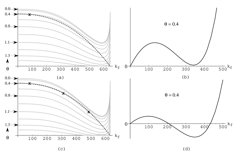
Figure 2: (a) The l.h.s. and r.h.s of Eq.(4.17) for the solution shown in Fig.1 are plotted here. The dark dashed line corresponds to the l.h.s of Eq.(4.17), and the gray lines to the r.h.s side for the indicated values of $\theta$. The intersection of these curves determines the numerical solution for $k_{f}(\theta)$. (b) This is a plot of the function $2m^{*}(dm^{*}/dk_{f})-2\mu^{*}(d\mu^{*}/dk_{f})-2k_{f}$, which is the l.h.s. of Eq.(5.1), for $\theta=0.4$. This shows why the solution in Fig.1 has minimum density, since for any higher values of $C_{V}^{2}$ and $C_{S}^{2}$ the function shown here would have negative values and, hence, the solution would be unphysical. (c),(d) Show the same as (a) and (b) respectively, but for an unphysical solution with the same binding energy, with parameters $C_{V}^{2}=.27\ \mbox{and}\ C_{S}^{2}=.77$, larger than $(C_{V}^{2})_{max}=.24$ and $(C_{S}^{2})_{max}=.62$ corresponding to the case in (a) and (b).

References

• [1] S. Weinberg, Phys. Rev. 166 (1668) 1568; S. Weinberg, Phys. Rev. Lett. 18 (1967) 188.
• [2] Howard Georgi, Weak Interactions and Modern Particle Theory, (The Benjamin/Cummings Publishing Company, Inc., 1984).
• [3] A. Manohar and H. Georgi, Nucl. Phys. B234 (1984) 189.
• [4] S. Coleman, J. Wess and B. Zumino, Phys. Rev. 177 (1968) 2239; C. Callan, S. Coleman, J. Wess and B. Zumino, Phys. Rev. 177 (1968) 2247.
• [5] D.B Kaplan and A.E. Nelson, Phys. Lett. B175 (1986) 57.
• [6] H.D. Politzer and M.B. Wise, Phys. Lett. B273 (1991) 156.
• [7] G.E Brown, K. Kubodera, M. Rho, and V. Thorsson, Phys. Lett. B291 355.
• [8] S. Bahcall, B. Lynn, and S.B. Selipsky, Nucl. Phys. B325 (1989) 606; J. Frieman and B.W. Lynn, Nucl. Phys. B329 (1990) 1; S. Bahcall, B. Lynn, and S.B. Selipsky, Nucl. Phys. B331 (1990) 67.
• [9] B. Lynn, Nucl. Phys. B402 (1993) 281.
• [10] B. Lynn, A. Nelson, and N. Tetradis, Nucl. Phys. B345 (1990) 186.
• [11] S.A. Chin and J.D. Walecka, Phys. Lett. B52 (1974) 24.
• [12] Private discussions with Hidonori Sonoda.
• [13] G. Gelmini and B. Ritzi, Phys. Lett. B357 (1995) 432.
• [14] H.A. Bethe, Phys. Rev 167 (1968) 879.
• [15] A.E.Nelson, Phys. Lett. b240 (1990) 179.