We have determined the theoretical predictions for the cross-sections of squark and gluino production at $p\bar{p}$ and $pp$ colliders (Tevatron and LHC) in next-to-leading order of supersymmetric QCD. By reducing the dependence on the renormalization/factorization scale considerably, the theoretically predicted values for the cross-sections are much more stable if these higher-order corrections are implemented. If squarks and gluinos are discovered, this improved stability translates into a reduced error on the masses, as extracted experimentally from the size of the production cross-sections. The cross-sections increase significantly if the next-to-leading order corrections are included at a renormalization/factorization scale near the average mass of the produced massive particles. This rise results in improved lower bounds on squark and gluino masses. By contrast, the shape of the transverse-momentum and rapidity distributions remains nearly unchanged when the next-to-leading order corrections are included.

1 Introduction

The supersymmetric extension of the Standard Model [1] is a well-motivated step. In supersymmetric theories the hierarchy problem of the Higgs sector can be solved [2]. Even in the context of very high energy scales, as required by grand unification, it is possible to retain fundamental scalar Higgs particles with low masses. This is a consequence of pairing bosons with fermions in supersymmetric multiplets, which removes the quadratic divergences due to these high scales from the quantum fluctuations. Moreover, the electroweak Higgs mechanism can be generated radiatively [3]. For a top mass in the experimentally observed range, the theory can evolve from a symmetric phase at the grand-unification scale to a phase of broken electroweak symmetry at low energies, while leaving the electromagnetic and colour gauge symmetry unbroken. Strong supporting evidence for supersymmetry is provided by the successful theoretical prediction of the electroweak mixing angle [4], $\sin^{2}\theta_{w}=0.2334\pm 0.0035$, based on the particle spectrum of the Minimal Supersymmetric extension of the Standard Model (MSSM). This prediction is matched quite well by the measured value [5], $\sin^{2}\theta_{w}^{\text{exp}}=0.2317\pm 0.0004$. Supersymmetric extensions offer solutions for many other problems that cannot be solved within the Standard Model [see e.g. Ref. [6] for a comprehensive discussion].

In the MSSM [7] quarks and leptons are paired with squarks and sleptons, gauge and Higgs particles with gauginos and higgsinos. Supersymmetric QCD (SUSY-QCD) is based on the coloured particles of this spectrum: quarks and spin-0 squarks ($\tilde{q}=\tilde{q}_{L},\tilde{q}_{R}$), gluons and spin-1/2 gluinos ($\tilde{g}$). The magnitude of the SUSY-QCD interactions is set by the gauge and Yukawa couplings $g_{s}$ and $\hat{g}_{s}=g_{s}$, respectively; the two couplings are required by supersymmetry to be equal. If supersymmetry were an exact symmetry, squarks and quarks would have equal masses and gluinos would be massless. However, supersymmetry is a broken symmetry, and the masses of the supersymmetric partners must exceed the masses of the Standard-Model particles considerably. Even though the mechanism for the breaking of supersymmetry is not identified yet at the fundamental level, requiring that no quadratic divergences be reintroduced into the theory by breaking the symmetry, provides a powerful guiding principle [8]. In this approach, supersymmetry is broken within SUSY-QCD by introducing heavy masses for squarks and gluinos, lifting the mass degeneracy with quarks and gluons. In order not to ruin the solution of the hierarchy problem, the masses of these particles should not exceed limits of ${\cal O}(1~{}\text{TeV})$.

In the present analysis we will assume that the scalar partners $\tilde{q}=(\tilde{q}_{L},\tilde{q}_{R})$ of the five light quark flavours are mass degenerate. We defer the discussion of final-state stop particles, with potentially significant L–R mixing due to the large top–Higgs Yukawa coupling, to a subsequent paper [9]. Stop masses in loop diagrams can be identified with the other squark masses since their impact is small. The masses of the five light quarks are neglected, while the top-quark mass is set to $m_{t}=175~{}\text{GeV}$. [The set of Feynman rules in SUSY-QCD, including an extensive discussion of the Majorana gluinos, is summarized in Appendix A; more details are given in Ref. [10].]

The search for supersymmetric particles ranks among the most important experimental endeavours of high-energy physics. The coloured particles, squarks and gluinos, can be searched for most efficiently at hadron colliders. As R parity is conserved in the QCD sector of $N=1$ supersymmetric theories, these particles are always produced in pairs. Squarks and gluinos decay primarily into cascades of jets plus the lightest supersymmetric particle (LSP), which escapes undetected. This particle is in general identified with the lightest neutralino $\tilde{\chi}_{1}^{0}$. Missing momentum is therefore one of the classical characteristics of SUSY events. Pairs of gluinos can decay into like-sign dileptons plus two LSPs, providing an almost background-free signal.

Squarks and gluinos can at present be searched for at the Fermilab Tevatron, a $p\bar{p}$ collider with a centre-of-mass energy of $1.8~{}\text{TeV}$, which will be upgraded to $2~{}\text{TeV}$ in the near future. Lower bounds on the squark and gluino masses have been set by both Tevatron experiments, CDF and D0 [11, 12]. At the 95% confidence level, the lower bound for the gluino mass is $173~{}\text{GeV}$, independent of the value of the squark mass. If squarks and gluinos have the same mass, the lower limit is given as $225~{}\text{GeV}$. Within the theoretical set-up of the experimental analysis, no limit for squark masses can be derived if the gluino mass exceeds $550~{}\text{GeV}$. [The lower limits on squark masses obtained at LEP are independent of this assumption.] This set of experimental bounds on squark and gluino production has been obtained in the framework of supergravity models, in which gluinos cannot be much heavier than squarks. If the supergravity relations are relaxed to the supersymmetric GUT relations between the gaugino masses, the excluded range in the gluino/squark-mass plane can be extended slightly. For gluino masses above $550~{}\text{GeV}$, no bound on the squark masses can be obtained any more, since the LSP $\tilde{\chi}_{1}^{0}$ becomes so heavy that the missing transverse momentum is insufficient to generate an observable signal. [Very light gluinos, which may have escaped detection at hadron colliders, are improbable in the light of the observed topologies of hadronic $Z$ decays; see e.g. Ref. [13]]. In the near future the search for squarks and gluinos can be extended at the upgraded Tevatron to masses between $300~{}\text{GeV}$ and $400~{}\text{GeV}$. At the $pp$ collider LHC the mass range up to $1.5$–$2~{}\text{TeV}$ can be sweeped, which covers the canonical range of the coloured supersymmetric particles, yet may not exhaust the parameter space entirely.

The cross-sections for the production of squarks and gluinos in hadron collisions were calculated at the Born level already quite some time ago [14]. Only recently have the predictions been improved by next-to-leading order (NLO) SUSY-QCD corrections for squark–antisquark [15] and gluino-pair production [16] in $p\bar{p}$ collisions. In the present paper we give a systematic analysis of the next-to-leading order SUSY-QCD corrections of all possible supersymmetric pair channels,

$$p\bar{p}/pp\longrightarrow\tilde{q}\tilde{q},\tilde{q}\bar{\tilde{q}},\tilde{q}\tilde{g},\tilde{g}\tilde{g}+X\quad(\tilde{q}\neq\tilde{t})$$ (1)

in the proton–antiproton collisions at the Tevatron and the proton–proton collisions at the LHC.

Several arguments demand the NLO SUSY-QCD analysis in order to obtain adequate theoretical predictions for the cross-sections:

(i) The lowest-order cross-sections depend strongly on the a priori unknown renormalization/factorization scale. As a result, the theoretical predictions are uncertain within factors of 2. By implementing the NLO corrections, this scale dependence is expected to be reduced significantly.

(ii) Drawing from the experience with similar hadronic processes [e.g. hadroproduction of top quarks], the NLO corrections are expected to be positive and large, thus enhancing the production cross-sections and raising the presently available (conservative) bounds on squark and gluino masses.

(iii) When squarks and gluinos will be discovered, the comparison of the measured total cross-sections with the theoretical predictions can be used to determine the masses of the particles. Due to the two escaping LSPs that are produced in the final-state decay cascades, the masses of squarks and gluinos cannot be determined by reconstructing the original squark and gluino states. [Transverse-momentum spectra can eventually be exploited to evaluate squark and gluino masses from the final-state distributions [18]].

Because of the large number of mechanisms, the calculation of the NLO corrections is tedious but straightforward. The only non-straightforward component of the theoretical set-up is one element of the renormalization program. To make maximal use of the common infrastructure developed earlier for top-quark production [17], we have chosen the $\overline{MS}$  renormalization scheme. However, this scheme leads in $n\neq 4$ dimensions to a mismatch between the 2 fermionic gluino degrees of freedom and the $(n-2)$ transverse gluon degrees of freedom. As a consequence, the gauge coupling $g_{s}(\overline{MS})$ and the Yukawa coupling $\hat{g}_{s}(\overline{MS})$ of the $\overline{MS}$  scheme differ in higher orders by a finite amount, even in exact supersymmetric theories. The problem, however, can be solved by introducing a proper counter term that restores the supersymmetry also in higher orders [19].

The paper is organized as follows. In the next section we recapitulate the lowest-order cross-sections for the partonic subprocesses of squark and gluino production for the sake of completeness and to define the notation. In Section 3 we carry out the calculation of the virtual SUSY-QCD corrections, followed by real-gluon radiation and the discussion of final states including light quarks. In Section 4 we present the overall corrections at the parton level and at the hadronic level for the total $p\bar{p}$ and $pp$ cross-sections. Furthermore, the transverse-momentum and rapidity distributions for semi-inclusive squark/gluino final states will be discussed briefly. We conclude the paper with an assessment of the results. Some useful technical details are collected in several Appendices.

2 Squark and Gluino Production in Leading Order

To set the stage for the subsequent discussion of higher-order effects, it is useful to recapitulate the lowest-order processes of squark and gluino production in quark and gluon collisions [14]. Moreover, the main features of the production mechanisms will be briefly described.

The hadroproduction of squarks and gluinos in leading order (LO) of the perturbative expansion proceeds through the following partonic reactions:

$$\tilde{q}\bar{\tilde{q}}\,\text{ production:}\quad q_{i} + \bar{q}_{j} \,\longrightarrow\, \tilde{q}_{k} + \bar{\tilde{q}}_{l}$$ (2)

$$g + g \,\longrightarrow\, \tilde{q}_{i} + \bar{\tilde{q}}_{i}$$ (3)

$$\tilde{q}\tilde{q}\,\text{ production:}\quad q_{i} + q_{j} \,\longrightarrow\, \tilde{q}_{i} + \tilde{q}_{j}\,\text{ and }c.c.$$ (4)

$$\tilde{g}\tilde{g}\,\text{ production:}\quad q_{i} + \bar{q}_{i} \,\longrightarrow\, \tilde{g} + \tilde{g}$$ (5)

$$g + g \,\longrightarrow\, \tilde{g} + \tilde{g}$$ (6)

$$\tilde{q}\tilde{g}\,\text{ production:}\quad q_{i} + g \,\longrightarrow\, \tilde{q}_{i} + \tilde{g}\,\text{ and }c.c.$$ (7)

The momenta of the two partons in the initial states are denoted by $k_{1}$ and $k_{2}$, those of the particles in the final states by $p_{1}$ and $p_{2}$.

The chiralities of the squarks $\tilde{q}=(\tilde{q}_{L},\tilde{q}_{R})$ are not noted explicitly. The indices $i$–$l$ indicate the flavours of the quarks and squarks. Also charge-conjugated processes ($c.c.$) are possible, related to the reactions (4) and (7); for the sake of simplicity they are not given explicitly. They will be taken into account properly when the hadronic cross-sections are calculated. The Feynman diagrams corresponding to these partonic reactions are displayed in Fig. 1.

Figure 1: Feynman diagrams for the production of squarks and gluinos in lowest order. The diagrams without and with crossed final-state lines [e.g. in (b)] represent $t$- and $u$-channel diagrams, respectively. The diagrams in (c) and the last diagram in (d) are a result of the Majorana nature of gluinos. Note that some of the above diagrams contribute only for specific flavours and chiralities of the squarks.

The production of squark–antisquark final states requires quark–antiquark (a) or gluon–gluon (b) initial states. Squark pairs can only be produced from quark-pair (c) initial states. Gluino pairs are produced from quark–antiquark (d) and gluon–gluon (e) initial states. The squark–gluino final states can only be produced in quark–gluon (f) collisions.

We use the Feynman gauge for the internal gluon propagators. For the external gluons only the transverse polarization states are generated. In the axial gauge the polarization sum for the external gluons is given by

$$P_{i}^{\mu\nu}=\sum_{T}\epsilon^{\mu\ast}_{T}(k_{i})\,\epsilon^{\nu}_{T}(k_{i})=-g^{\mu\nu}+\frac{n_{i}^{\mu}k_{i}^{\nu}+k_{i}^{\mu}n_{i}^{\nu}}{(n_{i}\,k_{i})}-\frac{n_{i}^{2}\,k_{i}^{\mu}k_{i}^{\nu}}{(n_{i}\,k_{i})^{2}}.$$ (8)

Here $n_{i}\neq k_{i}$ is an arbitrary vector. This polarization sum obeys the transversality relations

$$k_{i\mu}\,P_{i}^{\mu\nu}=P_{i}^{\mu\nu}k_{i\nu}=n_{i\mu}\,P_{i}^{\mu\nu}=P_{i}^{\mu\nu}n_{i\nu}=0.$$

Combining these transversality relations with the Slavnov–Taylor identities for on-shell external particles, e.g.

$$k_{i}^{\mu}M_{\mu\rho}=M^{ghost}_{\rho}\propto k_{j\rho}$$ (9)

for two external gluons [labelled $i$ and $j$], allows us to perform ghost subtraction. Because of the transversality relations all terms proportional to $k_{i}^{\mu}$ and $k_{j}^{\rho}$ can be removed from the LO matrix elements, resulting in the nullification of the right-hand side of Eq. (9) [ghost subtraction]. As a consequence, the polarization sum can effectively be replaced by $P_{i}^{\mu\nu}=-g^{\mu\nu}$.

The $n_{f}=5$ light quark flavours and the gluons are treated as massless particles. Since we have excluded the top-squarks from the final state, all squark-flavour and chirality states are considered to be mass degenerate with mass $m_{\tilde{q}}$. The gluino mass is denoted by $m_{\tilde{g}}$. The set of kinematical invariants used for the description of the reactions (2)–(7) is given by

$$s =(k_{1}+k_{2})^{2}$$ (11)

$$t =(k_{2}-p_{2})^{2} \qquad t_{1} =(k_{2}-p_{2})^{2}-m_{\tilde{q}}^{2} \qquad t_{g} =(k_{2}-p_{2})^{2}-m_{\tilde{g}}^{2}$$

$$u =(k_{1}-p_{2})^{2} \qquad u_{1} =(k_{1}-p_{2})^{2}-m_{\tilde{q}}^{2} \qquad u_{g} =(k_{1}-p_{2})^{2}-m_{\tilde{g}}^{2}.$$

The Mandelstam invariants are related by $s+t+u=p_{1}^{2}+p_{2}^{2}$. All in- and outgoing particles are assumed to be on their respective mass shells, i.e. $k_{i}^{2}=0$, $p_{i}^{2}=m_{\tilde{q}}^{2}$ for squarks, and $p_{i}^{2}=m_{\tilde{g}}^{2}$ for gluinos.

Applying the Feynman rules given in Appendix A, we obtain the following squared lowest-order matrix elements $|{\cal M}^{B}|^{2}$ in $n=4-2\varepsilon$ dimensions:

$$\sum|{\cal M}^{B}|^{2}(q_{i}\bar{q}_{j}\to\tilde{q}\bar{\tilde{q}}) = \delta_{ij}\left[8n_{f}g_{s}^{4}\,NC_{F}\,\frac{t_{1}u_{1}-m_{\tilde{q}}^{2}s}{s^{2}}+4\hat{g}_{s}^{4}\,NC_{F}\,\frac{t_{1}u_{1}-(m_{\tilde{q}}^{2}-m_{\tilde{g}}^{2})s}{t_{g}^{2}}\right.$$

$$\hphantom{\delta_{ij}a}\left.{}-8g_{s}^{2}\hat{g}_{s}^{2}\,C_{F}\,\frac{t_{1}u_{1}-m_{\tilde{q}}^{2}s}{st_{g}}\right]+(1-\delta_{ij})\left[4\hat{g}_{s}^{4}\,NC_{F}\,\frac{t_{1}u_{1}-(m_{\tilde{q}}^{2}-m_{\tilde{g}}^{2})s}{t_{g}^{2}}\right]$$

$$\sum|{\cal M}^{B}|^{2}(gg\to\tilde{q}\bar{\tilde{q}}) = \!\!4n_{f}g_{s}^{4}\left[C_{O}\!\left(1-2\,\frac{t_{1}u_{1}}{s^{2}}\right)-\!C_{K}\right]\!\left[1-\!\varepsilon-\!2\,\frac{sm_{\tilde{q}}^{2}}{t_{1}u_{1}}\left(1-\!\frac{sm_{\tilde{q}}^{2}}{t_{1}u_{1}}\right)\right]\quad\qquad$$

$$\sum|{\cal M}^{B}|^{2}(q_{i}q_{j}\to\tilde{q}\tilde{q}) = \delta_{ij}\Bigg{[}2\hat{g}_{s}^{4}\,NC_{F}\left(t_{1}u_{1}-m_{\tilde{q}}^{2}s\right)\left(\frac{1}{t_{g}^{2}}+\frac{1}{u_{g}^{2}}\right)$$

$${}\hphantom{\delta_{ij}a}+4\hat{g}_{s}^{4}\,m_{\tilde{g}}^{2}s\left(NC_{F}\left(\frac{1}{t_{g}^{2}}+\frac{1}{u_{g}^{2}}\right)-2C_{F}\,\frac{1}{t_{g}u_{g}}\right)\Bigg{]}$$

$${}+(1-\delta_{ij})\left[4\hat{g}_{s}^{4}\,NC_{F}\,\frac{t_{1}u_{1}-(m_{\tilde{q}}^{2}-m_{\tilde{g}}^{2})s}{t_{g}^{2}}\right]$$

$$\sum|{\cal M}^{B}|^{2}(q\bar{q}\to\tilde{g}\tilde{g}) = 4g_{s}^{4}\,C_{O}\left[\frac{2m_{\tilde{g}}^{2}s+t_{g}^{2}+u_{g}^{2}}{s^{2}}-\varepsilon\right]$$

$${}+4g_{s}^{2}\hat{g}_{s}^{2}\,C_{O}\left[\frac{m_{\tilde{g}}^{2}s+t_{g}^{2}}{st_{1}}+\frac{m_{\tilde{g}}^{2}s+u_{g}^{2}}{su_{1}}+\varepsilon\left(\frac{t_{g}}{t_{1}}+\frac{u_{g}}{u_{1}}\right)\right]$$

$${}+2\hat{g}_{s}^{4}\left[C_{O}\left(\frac{t_{g}^{2}}{t_{1}^{2}}+\frac{u_{g}^{2}}{u_{1}^{2}}\right)+C_{K}\left(2\,\frac{m_{\tilde{g}}^{2}s}{t_{1}\,u_{1}}-\frac{t_{g}^{2}}{t_{1}^{2}}-\frac{u_{g}^{2}}{u_{1}^{2}}\right)\right]$$

$$\sum|{\cal M}^{B}|^{2}(gg\to\tilde{g}\tilde{g}) = 8g_{s}^{4}\,NC_{O}\left(1-\frac{t_{g}u_{g}}{s^{2}}\right)\left[\frac{s^{2}}{t_{g}\,u_{g}}\left(1-\varepsilon\right)^{2}-2\left(1-\varepsilon\right)+4\,\frac{m_{\tilde{g}}^{2}s}{t_{g}u_{g}}\left(1-\frac{m_{\tilde{g}}^{2}s}{t_{g}u_{g}}\right)\right]$$

$$\sum|{\cal M}^{B}|^{2}(qg\to\tilde{q}\tilde{g}) = 2g_{s}^{2}\hat{g}_{s}^{2}\left[C_{O}\left(1-2\,\frac{su_{1}}{t_{g}^{2}}\right)-C_{K}\right]\Bigg{[}(-1+\varepsilon)\,\frac{t_{g}}{s}$$

$${}+\frac{2(m_{\tilde{g}}^{2}-m_{\tilde{q}}^{2})\,t_{g}}{su_{1}}\left(1+\frac{m_{\tilde{q}}^{2}}{u_{1}}+\frac{m_{\tilde{g}}^{2}}{t_{g}}\right)\Bigg{]}.$$

The QCD gauge coupling ($qqg$) is denoted by $g_{s}$ and the Yukawa coupling ($q\tilde{q}\tilde{g}$) by $\hat{g}_{s}$. These couplings are identical. For squarks all chiralities and non-stop flavours are summed over. As mentioned before, the charge-conjugate final states that are not denoted explicitly in the above listing, will be included in the hadronic cross-sections. The $SU(3)$ colour factors are given by $N=3$, $C_{O}=N(N^{2}-1)=24$, $C_{K}=(N^{2}-1)/N=8/3$, and $C_{F}=(N^{2}-1)/(2N)=4/3$.

After performing the $n$-dimensional phase-space integration and taking into account colour and spin averaging, we find for the lowest-order double-differential distributions:

$$s^{2}\,\frac{d^{2}\sigma^{B}}{dt\,du} = K_{ij}\,\frac{\pi S_{\varepsilon}}{\Gamma(1-\varepsilon)}\left[\frac{(t-p_{2}^{2})(u-p_{2}^{2})-p_{2}^{2}s}{\mu^{2}s}\right]^{-\varepsilon}\Theta(\,[t-p_{2}^{2}][u-p_{2}^{2}]-p_{2}^{2}s\,)$$ (12)

$$\times\,\Theta(s-4m^{2})\,\delta(s+t+u-p_{1}^{2}-p_{2}^{2})\sum|{\cal M}^{B}|^{2}.$$

Here $m$ denotes the average mass of the produced particles, i.e. $m=(\sqrt{p_{1}^{2}}+\sqrt{p_{2}^{2}}\,)/2$. The averaging of the initial-state colours and spins is incorporated in the factor $K_{ij}$:

$$K_{qq}=K_{q\bar{q}}=\frac{1}{4N^{2}},\qquad K_{gg}=\frac{1}{4(1-\varepsilon)^{2}(N^{2}-1)^{2}},\qquad K_{qg}=\frac{1}{4(1-\varepsilon)N(N^{2}-1)}.$$

The gluons have $(n-2)$ degrees of freedom in $n$ dimensions. The scale parameter $\mu$ accounts for the correct dimension of the coupling in $n$ dimensions. The term $S_{\varepsilon}=(4\pi)^{-2+\varepsilon}$ follows from the angular integrations.

The subsequent integration over the remaining invariants yields the total lowest-order partonic cross-sections [14]:

$$\sigma^{B}(q_{i}\bar{q}_{j}\to\tilde{q}\bar{\tilde{q}}) = \delta_{ij}\,\frac{n_{f}\pi\alpha_{s}^{2}}{s}\,\beta_{\tilde{q}}\left[\frac{4}{27}-\frac{16m_{\tilde{q}}^{2}}{27s}\right]$$

$${}+\delta_{ij}\,\frac{\pi\alpha_{s}\hat{\alpha}_{s}}{s}\left[\beta_{\tilde{q}}\left(\frac{4}{27}+\frac{8m_{-}^{2}}{27s}\right)+\left(\frac{8m_{\tilde{g}}^{2}}{27s}+\frac{8m_{-}^{4}}{27s^{2}}\right)L_{1}\right]$$

$${}+\frac{\pi\hat{\alpha}_{s}^{2}}{s}\left[\beta_{\tilde{q}}\left(-\frac{4}{9}-\frac{4m_{-}^{4}}{9(m_{\tilde{g}}^{2}s+m_{-}^{4})}\right)+\left(-\frac{4}{9}-\frac{8m_{-}^{2}}{9s}\right)L_{1}\right]$$

$$\sigma^{B}(gg\to\tilde{q}\bar{\tilde{q}}) = \frac{n_{f}\pi\alpha_{s}^{2}}{s}\left[\beta_{\tilde{q}}\left(\frac{5}{24}+\frac{31m_{\tilde{q}}^{2}}{12s}\right)+\left(\frac{4m_{\tilde{q}}^{2}}{3s}+\frac{m_{\tilde{q}}^{4}}{3s^{2}}\right)\log\left(\frac{1-\beta_{\tilde{q}}}{1+\beta_{\tilde{q}}}\right)\right]$$

$$\sigma^{B}(q_{i}q_{j}\to\tilde{q}\tilde{q}) = \frac{\pi\hat{\alpha}_{s}^{2}}{s}\left[\beta_{\tilde{q}}\left(-\frac{4}{9}-\frac{4m_{-}^{4}}{9(m_{\tilde{g}}^{2}s+m_{-}^{4})}\right)+\left(-\frac{4}{9}-\frac{8m_{-}^{2}}{9s}\right)L_{1}\right]$$

$${}+\delta_{ij}\,\frac{\pi\hat{\alpha}_{s}^{2}}{s}\left[\frac{8m_{\tilde{g}}^{2}}{27(s+2m_{-}^{2})}L_{1}\right]$$

$$\sigma^{B}(q\bar{q}\to\tilde{g}\tilde{g}) = \frac{\pi\alpha_{s}^{2}}{s}\,\beta_{\tilde{g}}\left(\frac{8}{9}+\frac{16m_{\tilde{g}}^{2}}{9s}\right)$$

$${}+\frac{\pi\alpha_{s}\hat{\alpha}_{s}}{s}\left[\beta_{\tilde{g}}\left(-\frac{4}{3}-\frac{8m_{-}^{2}}{3s}\right)+\left(\frac{8m_{\tilde{g}}^{2}}{3s}+\frac{8m_{-}^{4}}{3s^{2}}\right)L_{2}\right]$$

$${}+\frac{\pi\hat{\alpha}_{s}^{2}}{s}\left[\beta_{\tilde{g}}\left(\frac{32}{27}+\frac{32m_{-}^{4}}{27(m_{\tilde{q}}^{2}s+m_{-}^{4})}\right)+\left(-\frac{64m_{-}^{2}}{27s}-\frac{8m_{\tilde{g}}^{2}}{27(s-2m_{-}^{2})}\right)L_{2}\right]$$

$$\sigma^{B}(gg\to\tilde{g}\tilde{g}) = \frac{\pi\alpha_{s}^{2}}{s}\left[\beta_{\tilde{g}}\left(-3-\frac{51m_{\tilde{g}}^{2}}{4s}\right)+\left(-\frac{9}{4}-\frac{9m_{\tilde{g}}^{2}}{s}+\frac{9m_{\tilde{g}}^{4}}{s^{2}}\right)\log\left(\frac{1-\beta_{\tilde{g}}}{1+\beta_{\tilde{g}}}\right)\right]$$

$$\sigma^{B}(qg\to\tilde{q}\tilde{g}) = \frac{\pi\alpha_{s}\hat{\alpha}_{s}}{s}\,\left[\frac{\kappa}{s}\left(-\frac{7}{9}-\frac{32m_{-}^{2}}{9s}\right)+\left(-\frac{8m_{-}^{2}}{9s}+\frac{2m_{\tilde{q}}^{2}m_{-}^{2}}{s^{2}}+\frac{8m_{-}^{4}}{9s^{2}}\right)L_{3}\right.$$

$$\hphantom{\frac{\pi\alpha_{s}\hat{\alpha}_{s}}{s}a}\left.{}+\left(-1-\frac{2m_{-}^{2}}{s}+\frac{2m_{\tilde{q}}^{2}m_{-}^{2}}{s^{2}}\right)L_{4}\right],$$

with

$$L_{1} =\log\left(\frac{s+2m_{-}^{2}-s\beta_{\tilde{q}}}{s+2m_{-}^{2}+s\beta_{\tilde{q}}}\right) \qquad L_{2} =\log\left(\frac{s-2m_{-}^{2}-s\beta_{\tilde{g}}}{s-2m_{-}^{2}+s\beta_{\tilde{g}}}\right)$$

$$L_{3} =\log\left(\frac{s-m_{-}^{2}-\kappa}{s-m_{-}^{2}+\kappa}\right) \qquad L_{4} =\log\left(\frac{s+m_{-}^{2}-\kappa}{s+m_{-}^{2}+\kappa}\right)$$

$$\beta_{\tilde{q}} =\sqrt{1-\frac{4m_{\tilde{q}}^{2}}{s}} \qquad\beta_{\tilde{g}} =\sqrt{1-\frac{4m_{\tilde{g}}^{2}}{s}}$$

$$m_{-}^{2} =m_{\tilde{g}}^{2}-m_{\tilde{q}}^{2} \qquad\kappa =\sqrt{(s-m_{\tilde{g}}^{2}-m_{\tilde{q}}^{2})^{2}-4m_{\tilde{g}}^{2}m_{\tilde{q}}^{2}}$$

$$\alpha_{s} =g_{s}^{2}/4\pi \qquad\hat{\alpha}_{s} =\hat{g}_{s}^{2}/4\pi.$$

Note that we have suppressed the theta-functions $\Theta(s-4m^{2})$ for the production thresholds. For identical particles in the final state [gluino-pair production or production of squarks with identical chirality and flavour] a statistical factor $1/2$ has been taken into account.

For the production of squark pairs or squark–gluino pairs only one initial state contributes at lowest order. For squark–antisquark and gluino pairs both gluon–gluon and quark–antiquark initial states are possible.

The total hadronic cross-sections are obtained by integrating the parton cross-sections in the usual way over the parton distributions $f_{i}$ in the proton/antiproton:

$$\sigma(ij\to\tilde{q},\tilde{g})=\int\,dx_{1}\,dx_{2}\,f_{i}(x_{1})\,f_{j}(x_{2})\,\sigma^{B}(ij\to\tilde{q},\tilde{g};s=x_{1}x_{2}S),$$ (13)

where the total centre-of-mass energy of the collider is denoted by $\sqrt{S}$.

To assess the relative weights of $\tilde{q}\bar{\tilde{q}}$, $\tilde{q}\tilde{q}$, $\tilde{g}\tilde{g}$ and $\tilde{q}\tilde{g}$ final states in $p\bar{p}$ collisions at the Tevatron and in $pp$ collisions at the LHC, the relative yields are shown for a typical set of mass parameters in Fig. 2 and Fig. 3. The relative yields of squarks and gluinos in the final states depend strongly on the mass ratio $m_{\tilde{q}}/m_{\tilde{g}}$, for which we have chosen two representative values, $0.8$ and $1.6$. If squarks are lighter than gluinos, the valence partons give the dominant yield of squark–antisquark pairs/squark pairs at the Tevatron/LHC. By contrast, if the gluinos are the lighter of the two species, their production is the most copious.

Figure 2: The relative yields of squarks and gluinos in the final states at the Tevatron. The mass ratio $m_{\tilde{q}}/m_{\tilde{g}}$ is chosen to be (a) $0.8$ and (b) $1.6$. Also shown are the leading parton contributions for (c) $\tilde{q}\bar{\tilde{q}}$ and (d) $\tilde{g}\tilde{g}$ final states. Parton densities: GRV 94 [20]; renormalization and factorization scale $Q=m_{\tilde{q}}$ for squarks, $Q=m_{\tilde{g}}$ for gluinos, and $Q=(m_{\tilde{q}}+m_{\tilde{g}})/2$ for squark–gluino pairs.

Figure 3: The relative yields of squarks and gluinos in the final states at the LHC. The mass ratio $m_{\tilde{q}}/m_{\tilde{g}}$ is chosen to be (a) $0.8$ and (b) $1.6$. Also shown are the leading parton contributions for (d) $\tilde{g}\tilde{g}$ final states. Parton densities: GRV 94 [20]; renormalization and factorization scale $Q=m_{\tilde{q}}$ for squarks, $Q=m_{\tilde{g}}$ for gluinos, and $Q=(m_{\tilde{q}}+m_{\tilde{g}})/2$ for squark–gluino pairs. [Note that $\tilde{q}\tilde{q}/\tilde{q}\tilde{g}$ final states can only be generated by $qq/qg$ initial states so that diagram (c) is trivial and not shown.]

3 SUSY-QCD Corrections

3.1 Virtual Corrections

In this subsection we will present the virtual QCD corrections to the partonic production cross-sections of squarks and gluinos. The technical set-up of the calculation will be defined, including the renormalization of the ultraviolet (UV) divergences. The calculations are carried out in the $\overline{MS}$  renormalization scheme, which requires a careful analysis of the Yukawa ($q\tilde{q}\tilde{g}$) coupling $\hat{g}_{s}$ in higher orders.

3.1.1 Technical Set-Up

The calculation of the ${\cal O}(\alpha_{s})$ corrections to the reactions (2)–(7) involves the evaluation of the virtual corrections, i.e. the interference of the Born matrix element [after ghost subtraction] with the one-loop amplitudes. The corresponding differential cross-section is given by

$$s^{2}\,\frac{d^{2}\sigma^{V}}{dt\,du} = K_{ij}\,\frac{\pi S_{\varepsilon}}{\Gamma(1-\varepsilon)}\left[\frac{(t-p_{2}^{2})(u-p_{2}^{2})-p_{2}^{2}s}{\mu^{2}s}\right]^{-\varepsilon}\Theta(\,[t-p_{2}^{2}][u-p_{2}^{2}]-p_{2}^{2}s\,)$$ (14)

$$\times\,\Theta(s-4m^{2})\,\delta(s+t+u-p_{1}^{2}-p_{2}^{2})\sum\left({\cal M}^{B}{\cal M}^{V\ast}+{\cal M}^{V}{\cal M}^{B\ast}\right).$$

The virtual (one-loop) amplitudes include self-energy corrections, vertex corrections, and box diagrams. For the virtual particles inside loops we use the complete supersymmetric QCD spectrum: gluons, gluinos, all quarks, and all squarks. In Fig. 4 we present a set of typical virtual corrections.

Figure 4: A selected set of Feynman diagrams for the virtual corrections. (a) Gluino self-energy, (b) quark–quark–gluon vertex [gauge coupling], (c) quark–squark–gluino vertex [Yukawa coupling], (d) two-point boxes, (e) three-point boxes, and (f) four-point boxes.

In (a) the gluino self-energy is given. The diagram with reversed fermion-number flow contributes due to the Majorana nature of the gluinos. The vertex corrections are exemplified by a gauge vertex (b) and a Yukawa vertex (c). Typical examples for the different types of box diagrams are depicted in (d), (e), and (f).

The divergences in the virtual corrections are regularized by performing the calculations in $n=4-2\varepsilon$ dimensions. These divergences consist of ultraviolet, infrared (IR), and collinear divergences [also called mass singularities], and they show up as poles of the form $\varepsilon^{-i}$ ($i=1,2$). Since the virtual amplitudes are contracted with the Born matrix elements, all loop momenta will be contracted with themselves or external momenta. This leads to a great simplification of the tensor integrals appearing in the one-loop corrections. These tensor integrals are evaluated in $n$ dimensions by means of an adapted version of the standard Passarino–Veltman tensor integral reduction [21], and they are expressed in terms of scalar integrals. The coefficients of these scalar integrals are finite, and they have to be calculated up to ${\cal O}(\varepsilon^{2})$. The divergences are contained in the scalar integrals. We have calculated these, using two different techniques. One is based on the Feynman parametrization, the other proceeds via the computation of the absorptive part by applying the Cutkosky cutting rules in $n$ dimensions, followed by the use of dispersion-integral techniques to get the real part. All analytical manipulations were performed with the help of the symbolic computer program FORM [22].

The case of equal masses for squarks and gluinos is calculated separately, in view of additional singularities. Divergent terms of the form $\log[(m_{\tilde{g}}^{2}-m_{\tilde{q}}^{2})/m_{\tilde{q}}^{2}]$ lead to additional $1/\varepsilon$ poles. It has been checked explicitly that the final cross-sections are nevertheless continuous at this point of the mass-parameter space.

The singularity structure of the scalar integrals in $n$ dimensions can be summarized as follows. The non-vanishing scalar one-point and two-point functions only give rise to UV poles. The derivative of the on-shell two-point functions, and the three- and four-point functions are UV finite and give rise only to IR and collinear singularities. IR poles appear when a massless particle is exchanged between two on-shell particles; collinear poles show up when a massless particle splits into two massless collinear particles. Double poles are generated only when IR and collinear singularities are present at the same time.

The $\gamma_{5}$ Dirac matrix, entering the calculation through the quark–squark–gluino Yukawa couplings, is treated in the ‘naive’ scheme. In this scheme the $\gamma_{5}$-matrix anticommutes with the other $\gamma_{\mu}$-matrices. This is a legitimate procedure at the one-loop level for anomaly-free theories.

We have excluded the top-squarks from the final states, as discussed in the introduction. However, to carry out the NLO calculation consistently, we have to take into account the top-squarks inside loops. For the sake of simplicity we take them to be mass degenerate with the other squarks. For the top quark we use the mass $m_{t}=175~{}\text{GeV}$. Thus, the final results will depend on two free parameters: the squark mass $m_{\tilde{q}}$ and the gluino mass $m_{\tilde{g}}$.

The definitions of the invariant energies and momentum transfers, and the gauge choices for internal and external gluons are the same as in lowest order. Faddeev–Popov ghost contributions have therefore to be taken into account in the gluon self-energy and in the three-gluon vertex corrections.

3.1.2 Renormalization of UV Divergences

The UV divergences can be removed by renormalizing the coupling constants and the masses of the heavy particles. The external self-energies are multiplied by a factor $1/2$ to properly account for the transition from Green’s functions to the S-matrix. For the renormalization of the QCD coupling constant one usually resorts to the $\overline{MS}$ scheme, which involves $n$-dimensional regularization, i.e. fields, phase space, and loop momenta are defined in $n$ dimensions. The UV $1/\varepsilon$ poles are subtracted, together with specific transcendental constants, at an arbitrary subtraction point $Q_{R}$, the charge-renormalization scale.

In supersymmetric theories, however, a complication occurs. In $n\neq 4$ dimensions the $\overline{MS}$  scheme introduces a mismatch between the number of gluon ($n-2$) and gluino (2) degrees of freedom. Since this ${\cal O}(\varepsilon)$ mismatch will result in finite non-zero contributions, the $\overline{MS}$  scheme violates supersymmetry explicitly in higher orders. In particular, the Yukawa coupling $\hat{g}_{s}$, which by supersymmetry should coincide with the gauge coupling $g_{s}$, deviates from it by a finite amount at the one-loop level. Requiring the physical amplitudes to preserve this supersymmetric relation, a shift between the bare Yukawa coupling and the bare gauge coupling must be introduced in the $\overline{MS}$  scheme:

$$\hat{g}_{s}=g_{s}\left[1+\frac{\alpha_{s}}{4\pi}\left(\frac{2}{3}N-\frac{1}{2}C_{F}\right)\right]=g_{s}\left[1+\frac{\alpha_{s}}{3\pi}\right],$$ (15)

which effectively subtracts the contributions of the false, non-supersymmetric degrees of freedom [also called $\varepsilon$ scalars].

The need for introducing a finite shift is best demonstrated for the effective [one-loop corrected] Yukawa coupling, which must be equal to the effective gauge coupling in an exact supersymmetric world with massless gluons/gluinos and equal-mass quarks/squarks. For the sake of simplicity we define the effective couplings ${\Gamma}^{\text{eff}}(Q^{2})$ and $\hat{\Gamma}^{\text{eff}}(Q^{2})$ in the limit of on-shell quarks/squarks and almost on-shell gluons/gluinos, with virtuality $Q^{2}\ll m_{\tilde{q}}^{2}=m_{q}^{2}$; in this limit the couplings do not contain gauge-dependent terms. In the $\overline{MS}$  scheme we find, after charge renormalization:

$$\overline{MS}:\,{\Gamma}^{\text{eff}}(Q^{2})\! = \!g_{s}\left\{1+\frac{\alpha_{s}}{4\pi}\,N\,\left[-\frac{1}{\bar{\varepsilon}}-\log\left(\frac{\mu^{2}}{m_{\tilde{q}}^{2}}\right)-\frac{1}{2}\,\log\left(\frac{Q^{2}}{m_{\tilde{q}}^{2}}\right)+\frac{7}{6}\right]\right\}$$ (16)

$$\hat{\Gamma}^{\text{eff}}(Q^{2})\! = \!\hat{g}_{s}\left\{1+\frac{\alpha_{s}}{4\pi}\,\left(N\,\left[-\frac{1}{\bar{\varepsilon}}-\log\left(\frac{\mu^{2}}{m_{\tilde{q}}^{2}}\right)-\frac{1}{2}\,\log\left(\frac{Q^{2}}{m_{\tilde{q}}^{2}}\right)+\frac{1}{2}\right]+\frac{C_{F}}{2}\right)\right\}.$$ (17)

The singular term $1/\bar{\varepsilon}$ represents the combination $1/\varepsilon-\gamma_{E}+\log(4\pi)$. The remaining $1/\varepsilon$ poles are IR and collinear singularities. Inspecting ${\Gamma}^{\text{eff}}$ and $\hat{\Gamma}^{\text{eff}}$, it is easy to prove that the difference between the two effective couplings coincides with the shift in Eq. (15). Taking into account this finite shift of the bare couplings in the $\overline{MS}$  scheme, both effective couplings become identical at the one-loop level. In this way supersymmetry is preserved and the $\overline{MS}$  renormalization becomes a consistent scheme.

An alternative renormalization scheme is the modified Dimensional Reduction ($\overline{DR}$  ) scheme in which the fields are treated in four dimensions, but the phase space and loop momenta in $n$ dimensions. In this scheme no mismatch between bosonic and fermionic degrees of freedom is apparently introduced and supersymmetry is preserved ab initio. At the level of the effective couplings ${\Gamma}^{\text{eff}}$ and $\hat{\Gamma}^{\text{eff}}$, this is reflected in the equalities

$$\overline{DR}:\quad{\Gamma}^{\text{eff}}(Q^{2}) = g_{s}\left\{1+\frac{\alpha_{s}}{4\pi}\,N\,\left[-\frac{1}{\bar{\varepsilon}}-\log\left(\frac{\mu^{2}}{m_{\tilde{q}}^{2}}\right)-\frac{1}{2}\,\log\left(\frac{Q^{2}}{m_{\tilde{q}}^{2}}\right)+1\right]\right\}$$ (18)

$$= \hat{\Gamma}^{\text{eff}}(Q^{2}).$$ (19)

As a result, both couplings are identical order by order. [It should be noted that the transition from the effective gauge coupling in $\overline{MS}$  to the gauge coupling in $\overline{DR}$  involves a well-known finite renormalization $\alpha_{s}N/(24\pi)=\alpha_{s}/(8\pi)$ [23].]

In the following we use the $\overline{MS}$  renormalization scheme, supplemented by the finite shift of the Yukawa coupling. In this way supersymmetry is preserved on the one hand, while on the other hand the definition of the strong gauge coupling corresponds to the usual Standard-Model measurements.

Below we list the various renormalizations needed for the production of squarks and gluinos. In order to preserve the form of the Ward identity given in Eq. (9), non-zero particle masses have to be renormalized in an on-shell scheme. We have opted for a real mass renormalization, involving the subtraction of the real part of the on-shell self-energies at the real-valued pole masses. In the case of squarks and gluinos, this is equivalent to replacing the bare masses in the lowest-order propagators by

$$\left(m_{\tilde{q}}^{2}\right)^{bare} \to m_{\tilde{q}}^{2}\left\{1+\frac{\alpha_{s}}{4\pi}\,C_{F}\left[\left(-\frac{1}{\bar{\varepsilon}}-\log\left(\frac{\mu^{2}}{m_{\tilde{q}}^{2}}\right)\right)\left(\,4\frac{m_{\tilde{g}}^{2}}{m_{\tilde{q}}^{2}}\right)\right.\right.$$

$$\left.\left.-2-6\,\frac{m_{\tilde{g}}^{2}}{m_{\tilde{q}}^{2}}+\left(2-4\,\frac{m_{\tilde{g}}^{2}}{m_{\tilde{q}}^{2}}\right)\log\left(\frac{m_{\tilde{q}}^{2}}{m_{\tilde{g}}^{2}}\right)+\left(-2+4\,\frac{m_{\tilde{g}}^{2}}{m_{\tilde{q}}^{2}}-2\,\frac{m_{\tilde{g}}^{4}}{m_{\tilde{q}}^{4}}\right)\log\left|1-\frac{m_{\tilde{q}}^{2}}{m_{\tilde{g}}^{2}}\right|\,\right]\right\}$$

$$\left(m_{\tilde{g}}\right)^{bare} \to m_{\tilde{g}}\left\{1+\frac{\alpha_{s}}{4\pi}\left[\left(-\frac{1}{\bar{\varepsilon}}-\log\left(\frac{\mu^{2}}{m_{\tilde{g}}^{2}}\right)\right)\left(\,3N-n_{f}-1\right)\right.\right.$$

$$-4N+\frac{m_{\tilde{q}}^{2}}{m_{\tilde{g}}^{2}}-\frac{m_{t}^{2}}{m_{\tilde{g}}^{2}}+n_{f}\left(2-\frac{m_{\tilde{q}}^{2}}{m_{\tilde{g}}^{2}}\right)+\left(-n_{f}-\frac{m_{\tilde{q}}^{2}}{m_{\tilde{g}}^{2}}\right)\log\left(\frac{m_{\tilde{q}}^{2}}{m_{\tilde{g}}^{2}}\right)+\frac{m_{t}^{2}}{m_{\tilde{g}}^{2}}\log\left(\frac{m_{t}^{2}}{m_{\tilde{g}}^{2}}\right)$$

$$\left.\left.+n_{f}\left(-1+2\,\frac{m_{\tilde{q}}^{2}}{m_{\tilde{g}}^{2}}-\frac{m_{\tilde{q}}^{4}}{m_{\tilde{g}}^{4}}\right)\log\left|1-\frac{m_{\tilde{g}}^{2}}{m_{\tilde{q}}^{2}}\right|+\left(1-\frac{m_{\tilde{q}}^{2}}{m_{\tilde{g}}^{2}}+\frac{m_{t}^{2}}{m_{\tilde{g}}^{2}}\right)B_{0}\,\right]\right\},$$

with

$$B_{0} = {\cal\text{Re}}\,\left[\vphantom{\frac{1}{2}}2-\log\left(\frac{m_{\tilde{q}}^{2}}{m_{\tilde{g}}^{2}}\right)+x_{1}\log(1-1/x_{1})+x_{2}\log(1-1/x_{2})\right]$$

$$x_{1,2} = \frac{1}{2m_{\tilde{g}}^{2}}\left[m_{\tilde{g}}^{2}+m_{t}^{2}-m_{\tilde{q}}^{2}\pm\sqrt{(m_{\tilde{g}}^{2}-m_{t}^{2}-m_{\tilde{q}}^{2})^{2}-4m_{t}^{2}m_{\tilde{q}}^{2}}\,\right].$$

The parameters $m_{\tilde{q}}$ and $m_{\tilde{g}}$ are the pole masses.

As discussed above, the couplings are renormalized in the $\overline{MS}$  scheme, including the finite shift of the bare Yukawa coupling given by Eq. (15). This leads to the following replacements of the bare couplings in the LO expressions:

$$\left(g_{s}\right)^{bare} \to g_{s}(Q_{R}^{2})\left\{1+\frac{\alpha_{s}(Q_{R}^{2})}{4\pi}\left[\left(-\frac{1}{\bar{\varepsilon}}+\log\left(\frac{Q_{R}^{2}}{\mu^{2}}\right)\right)\frac{\beta_{0}}{2}\right.\right.$$

$$\hskip 42.67912pt\left.\left.-\frac{N}{3}\log\left(\frac{m_{\tilde{g}}^{2}}{Q_{R}^{2}}\right)-\frac{n_{f}+1}{6}\log\left(\frac{m_{\tilde{q}}^{2}}{Q_{R}^{2}}\right)-\frac{1}{3}\log\left(\frac{m_{t}^{2}}{Q_{R}^{2}}\right)\right]\right\}$$

$$\left(\hat{g}_{s}\right)^{bare} \to g_{s}(Q_{R}^{2})\left\{1+\frac{\alpha_{s}(Q_{R}^{2})}{4\pi}\left[\left(-\frac{1}{\bar{\varepsilon}}+\log\left(\frac{Q_{R}^{2}}{\mu^{2}}\right)\right)\frac{\beta_{0}}{2}\right.\right.$$

$$\hskip 42.67912pt\left.\left.-\frac{N}{3}\log\left(\frac{m_{\tilde{g}}^{2}}{Q_{R}^{2}}\right)-\frac{n_{f}+1}{6}\log\left(\frac{m_{\tilde{q}}^{2}}{Q_{R}^{2}}\right)-\frac{1}{3}\log\left(\frac{m_{t}^{2}}{Q_{R}^{2}}\right)+\frac{2N}{3}-\frac{C_{F}}{2}\right]\right\}.$$

The first coefficient $\beta_{0}$ of the SUSY-QCD $\beta$ function can be decomposed into a sum of contributions from light and heavy particles:

$$\beta_{0}=\left[\frac{11}{3}N-\frac{2}{3}n_{f}\right]+\left[-\frac{2}{3}N-\frac{2}{3}-\frac{1}{3}(n_{f}+1)\right]=\beta_{0}^{L}+\beta_{0}^{H}.$$ (20)

In addition to the poles, also some logarithms are subtracted in order to decouple the heavy particles [top quark, squarks, gluinos] from the running of $\alpha_{s}(Q_{R}^{2})$. In this decoupling scheme the $Q_{R}^{2}$ evolution of the strong coupling is determined completely by the light-particle spectrum [gluons and $n_{f}=5$ massless quarks]:

$$\frac{\partial\,g_{s}^{2}(Q_{R}^{2})}{\partial\log(Q_{R}^{2})}=g_{s}(Q_{R}^{2})\beta(g_{s})=-\alpha_{s}^{2}(Q_{R}^{2})\,\beta_{0}^{L}.$$ (21)

The methods described above to renormalize the UV divergences lead to cross-sections that are UV-finite. Nevertheless, there are still divergences left. The IR divergences will cancel against the contribution from soft-gluon radiation. The collinear singularities, finally, will be removed by applying mass factorization. These steps will be discussed in detail in the next subsections.

3.2 Real-Gluon Radiation

Two important aspects of the real-gluon radiation, the split-up of the phase space in soft- and hard-gluon regimes, and the renormalization of collinear divergences by means of mass factorization, will be discussed in detail in the following subsections.

3.2.1 Matrix Elements and Phase Space

In order to complete the NLO evaluation of squark and gluino production we need, in addition to the afore-mentioned virtual SUSY-QCD corrections, also the corrections from real-gluon radiation. They are obtained from the LO partonic reactions by adding a gluon to the final state:

$$q_{i} + \bar{q}_{j} \,\longrightarrow\, \tilde{q}_{k} + \bar{\tilde{q}}_{l} + g$$ (22)

$$g + g \,\longrightarrow\, \tilde{q}_{i} + \bar{\tilde{q}}_{i} + g$$ (23)

$$q_{i} + q_{j} \,\longrightarrow\, \tilde{q}_{i} + \tilde{q}_{j} + g$$ (24)

$$q_{i} + \bar{q}_{i} \,\longrightarrow\, \tilde{g} + \tilde{g} + g$$ (25)

$$g + g \,\longrightarrow\, \tilde{g} + \tilde{g} + g$$ (26)

$$q_{i} + g \,\longrightarrow\, \tilde{q}_{i} + \tilde{g} + g.$$ (27)

Again, the momenta of the initial-state partons are denoted by $k_{1},k_{2}$, while the particles in the final states carry momenta $p_{1},p_{2}$, and $k_{3}$. The charge-conjugate final states, which are not given here explicitly, will be taken into account when the hadronic cross-sections are calculated. A representative set of Feynman diagrams, contributing to the real-gluon amplitude ${\cal M}^{R}$, is given in Fig. 5.

Figure 5: A representative set of Feynman diagrams corresponding to real-gluon radiation: squark–antisquark production (a), gluino-pair production (b), and squark–gluino production (c).

We display some diagrams for (a) squark–antisquark production in quark–antiquark annihilation, (b) gluino-pair production in gluon fusion, and (c) squark–gluino production in quark–gluon collisions. The internal and external gluon lines, and the $\gamma_{5}$ Dirac matrix, are treated in the same way as before.

To evaluate the squared real-gluon matrix elements $|{\cal M}^{R}|^{2}$ we define the following kinematical invariants [17]:

$$s =(k_{1}+k_{2})^{2}\qquad\quad s_{5} =(p_{1}+p_{2})^{2}$$ (29)

$$s_{3} =(k_{3}+p_{2})^{2}-m_{\tilde{q}}^{2}\qquad\quad s_{4} =(k_{3}+p_{1})^{2}-m_{\tilde{q}}^{2}$$

$$t =(k_{2}-p_{2})^{2}\qquad\quad t^{\prime} =(k_{2}-k_{3})^{2}$$

$$u =(k_{1}-p_{2})^{2}\qquad\quad u^{\prime} =(k_{1}-k_{3})^{2}$$

$$u_{6} =(k_{2}-p_{1})^{2}-m_{\tilde{q}}^{2} \qquad\quad u_{7} =(k_{1}-p_{1})^{2}-m_{\tilde{q}}^{2}.$$

For the sake of convenience we will use the following additional invariants:

$$s_{3g} =s_{3}+m_{\tilde{q}}^{2}-m_{\tilde{g}}^{2}\qquad\quad s_{4g} =s_{4}+m_{\tilde{q}}^{2}-m_{\tilde{g}}^{2}$$

$$s_{4x} =s_{4}+m_{\tilde{q}}^{2}-p_{1}^{2}=2(k_{3}\,p_{1})\qquad$$

$$t_{1} =t-m_{\tilde{q}}^{2}\qquad\quad t_{g} =t-m_{\tilde{g}}^{2}$$

$$u_{1} =u-m_{\tilde{q}}^{2}\qquad\quad u_{g} =u-m_{\tilde{g}}^{2}$$

$$u_{6g} =u_{6}+m_{\tilde{q}}^{2}-m_{\tilde{g}}^{2}\qquad\quad u_{7g} =u_{7}+m_{\tilde{q}}^{2}-m_{\tilde{g}}^{2}.$$

The squared matrix elements must be evaluated in $n=4-2\varepsilon$ dimensions up to ${\cal O}(\varepsilon^{2})$.

After performing the $n$-dimensional three-particle phase-space integration, we find for the double-differential distributions

$$s^{2}\,\frac{d^{2}\sigma^{R}}{dt\,du} = K_{ij}\,\frac{S_{\varepsilon}^{2}\mu^{2\varepsilon}}{2\Gamma(1-2\varepsilon)}\left[\frac{(t-p_{2}^{2})(u-p_{2}^{2})-p_{2}^{2}s}{\mu^{2}s}\right]^{-\varepsilon}\Theta(\,[t-p_{2}^{2}][u-p_{2}^{2}]-p_{2}^{2}s\,)$$ (30)

$$\times\,\Theta(s-4m^{2})\,\frac{(2k_{3}p_{1})^{1-2\varepsilon}}{(2k_{3}p_{1}+p_{1}^{2})^{1-\varepsilon}}\,\Theta(2k_{3}p_{1})\int d\Omega_{n}\sum|{\cal M}^{R}|^{2},$$

with $2(k_{3}p_{1})=s+t+u-p_{1}^{2}-p_{2}^{2}\geq 0$. The $n$-dimensional angular integration is given explicitly by $\int d\Omega_{n}=\int_{0}^{\pi}\sin^{1-2\varepsilon}(\theta_{1})\,d\theta_{1}\,\int_{0}^{\pi}\sin^{-2\varepsilon}(\theta_{2})\,d\theta_{2}$ [see Appendix B]. To perform the angular integrations, we isolate the coefficients of the form $(s^{\prime})^{k}(s^{\prime\prime})^{l}$. The variables $s^{\prime}$ and $s^{\prime\prime}$ denote kinematical invariants of the list in Eq. (29), and $k$ and $l$ are integer numbers. One of those invariants should contain both integration variables ($\theta_{1},\theta_{2}$), whereas the second should depend only on $\theta_{1}$. This can be achieved by means of partial fractioning, exploiting the fact that only five of the kinematical invariants are in fact independent. The angular integrals are therefore of the form

$$I_{n}^{(k,l)}=\int_{0}^{\pi}\sin^{1-2\varepsilon}(\theta_{1})\,d\theta_{1}\,\int_{0}^{\pi}\sin^{-2\varepsilon}(\theta_{2})\,d\theta_{2}(a\!+\!b\cos\theta_{1})^{-k}(A\!+\!B\cos\theta_{1}\!+\!C\sin\theta_{1}\cos\theta_{2})^{-l}.$$ (31)

Explicit analytical expressions for these angular integrals can be found in Ref. [17]. In Appendix B we demonstrate how the kinematical invariants can be expressed in terms of the angular variables.

3.2.2 Soft- and Hard-Gluon Radiation

To identify the IR singularities, the phase space for gluon radiation is split into two distinct regimes, one describing soft gluons and the other describing hard gluons. This separation can be defined by introducing a cut-off parameter $\Delta$ in the invariant mass $s_{4x}=2(k_{3}p_{1})$, corresponding to the radiated gluon and one of the heavy particles in the final state. The cut-off parameter is chosen so small that it can be neglected with respect to any other mass scale in the process. In terms of the single-differential distribution $d\sigma/dt$ the split-up takes the form

$$\frac{d\sigma^{R}}{dt}=\int_{0}^{s_{4x}^{max}}ds_{4x}\,\frac{d^{2}\sigma^{R}}{dt\,du}=\int_{0}^{\Delta}ds_{4x}\,\frac{d^{2}\sigma^{S}}{dt\,du}+\int_{\Delta}^{s_{4x}^{max}}ds_{4x}\,\frac{d^{2}\sigma^{H}}{dt\,du}.$$ (32)

The first term on the right-hand side of Eq. (32) represents the regime of soft-gluon radiation. In this regime the momentum of the radiated gluon, $k_{3}$, tends to zero and an eikonal approximation can be applied, i.e. neglecting $k_{3}$ whenever possible. In the limit $k_{3}\to 0$, the $(2\to 3)$ kinematics is reduced to $(2\to 2)$ kinematics, and the kinematical invariants of Eq. (29) take the form

$$s_{5} \to s \qquad 2(k_{3}p_{1}) \to 0 \qquad 2(k_{3}p_{2}) \to 0 \qquad t^{\prime} \to 0$$ (34)

$$u^{\prime} \to 0 \qquad u_{6}/u_{6g} \to u_{1}/u_{g} \qquad u_{7}/u_{7g} \to t_{1}/t_{g},$$

while the remaining invariants are not affected.

After integration over the angles and over the invariant mass $s_{4x}$, singular expressions of the form $\varepsilon^{-i}$ $(i=1,2)$ are generated. The double poles correspond to configurations where IR and collinear singularities coincide. When the single-differential soft-gluon distribution $d\sigma^{S}/dt$ is added to the virtual corrections, the sum is IR-finite. This sum, however, is not free of divergences until the collinear singularities are removed by means of mass factorization.

The second term on the right-hand side of Eq. (32) represents the regime of hard-gluon radiation. In this regime only collinear singularities occur, generated when the radiated gluon is collinear with one of the initial-state massless particles. They show up in $|{\cal M}^{R}|^{2}$ as terms proportional to $1/t^{\prime}$ or $1/u^{\prime}$, which behave as $1/[1\pm\cos(\theta_{i})]$  $(i=1,2$) and lead to $1/\varepsilon$ poles after the angular integration. Also these collinear singularities have to be removed by means of mass factorization.

As a result of the split-up of the phase space, terms of the form $\log^{i}(\Delta/m^{2})$ $(i=1,2)$ occur in both the soft and hard cross-sections. They come from the same terms that generate the IR singularities. If soft and hard contributions are added up, however, any $\Delta$ dependence disappears from the cross-sections in the limit $\Delta\to 0$.

3.2.3 Mass Factorization

The collinear divergences, generated by the radiation of gluons [or massless quarks], have a universal structure. The partonic cross-sections $\sigma_{ij}$, which contain the collinear singularities, have the following form, factorized to all orders of perturbation theory:

$$s^{2}\,\frac{d^{2}\sigma_{ij}(s,t_{x},u_{x},\mu^{2},\varepsilon)}{dt_{x}\,du_{x}} = \int_{0}^{1}\frac{dx_{1}}{x_{1}}\int_{0}^{1}\frac{dx_{2}}{x_{2}}\sum_{l,m}\Gamma_{li}(x_{1},Q_{F}^{2},\mu^{2},\varepsilon)\,\Gamma_{mj}(x_{2},Q_{F}^{2},\mu^{2},\varepsilon)$$ (35)

$$\times\,\hat{s}^{2}\,\frac{d^{2}\hat{\sigma}_{lm}(\hat{s},\hat{t}_{x},\hat{u}_{x},Q_{F}^{2})}{d\hat{t}_{x}\,d\hat{u}_{x}}$$

$$t_{x}=-2(k_{2}p_{2})\quad u_{x}=-2(k_{1}p_{2})\quad\hat{s}=x_{1}x_{2}s\quad\hat{t}_{x}=x_{2}t_{x}\quad\hat{u}_{x}=x_{1}u_{x}.$$

The indices $i$–$m$ characterize the initial-state partons. The universal splitting functions $\Gamma_{ij}$, representing the probability of finding, inside the parent particle $j$ at the scale $Q_{F}^{2}$, a particle $i$ with fraction $x$ of the longitudinal momentum, contain the collinear divergences. They can be absorbed into a redefinition of the parton densities at NLO [24], in general called mass factorization. Since the subtraction point of the mass-factorization procedure is arbitrary, the splitting functions will depend on the factorization scale $Q_{F}$. Adopting the $\overline{MS}$  mass-factorization scheme we can write to ${\cal O}(\alpha_{s})$

$$\Gamma_{ij}(x,Q_{F}^{2},\mu^{2},\varepsilon)=\delta_{ij}\,\delta(1-x)+\frac{\alpha_{s}}{2\pi}\left[-\frac{1}{\bar{\varepsilon}}+\log\left(\frac{Q_{F}^{2}}{\mu^{2}}\right)\right]P_{ij}(x),\qquad$$ (36)

with $1/\bar{\varepsilon}=1/\varepsilon-\gamma_{E}+\log(4\pi)$ as before. The hard-scattering (reduced) cross-sections $\hat{\sigma}_{ij}$ are free of collinear divergences. They depend, like the splitting functions, on the scale $Q_{F}$. In NLO they have the form

$$s^{2}\,\frac{d^{2}\hat{\sigma}_{ij}(s,t_{x},u_{x},Q_{F}^{2})}{dt_{x}\,du_{x}} = s^{2}\,\frac{d^{2}{\sigma}_{ij}(s,t_{x},u_{x},\mu^{2},\varepsilon)}{dt_{x}\,du_{x}}$$

$$-\frac{\alpha_{s}}{2\pi}\int_{0}^{1}\frac{dx_{1}}{x_{1}}\left[-\frac{1}{\bar{\varepsilon}}+\log\left(\frac{Q_{F}^{2}}{\mu^{2}}\right)\right]P_{li}(x_{1})\,(x_{1}s)^{2}\,\frac{d^{2}{\sigma}^{B}_{lj}(x_{1}s,t_{x},x_{1}u_{x},\mu^{2},\varepsilon)}{dt_{x}\,d(x_{1}u_{x})}$$

$$-\frac{\alpha_{s}}{2\pi}\int_{0}^{1}\frac{dx_{2}}{x_{2}}\left[-\frac{1}{\bar{\varepsilon}}+\log\left(\frac{Q_{F}^{2}}{\mu^{2}}\right)\right]P_{kj}(x_{2})\,(x_{2}s)^{2}\,\frac{d^{2}{\sigma}^{B}_{ik}(x_{2}s,x_{2}t_{x},u_{x},\mu^{2},\varepsilon)}{d(x_{2}t_{x})\,du_{x}}.$$

The Altarelli–Parisi kernels $P_{ij}(x)$ [25] are given by [$T_{f}=1/2$]

$$P_{gg}(x,\delta) = 2N\left[\frac{1}{x(1-x)}+x(1-x)-2\right]\Theta(1-x-\delta)$$

$${}+\left[2N\log\delta+\frac{1}{2}\beta_{0}^{L}\right]\delta(1-x)$$

$$P_{qq}(x,\delta) = C_{F}\,\frac{1+x^{2}}{1-x}\,\Theta(1-x-\delta)+C_{F}\left[2\log\delta+\frac{3}{2}\right]\delta(1-x)$$ (39)

$$P_{gq}(x) = C_{F}\,\frac{1+(1-x)^{2}}{x}$$ (40)

$$P_{qg}(x) = T_{f}\left[x^{2}+(1-x)^{2}\right].$$ (41)

The parameter $\delta$ is related to the IR cut-off parameter $\Delta$ through relations of the form $\delta=\Delta/(s+t_{x})$ or $\delta=\Delta/(s+u_{x})$, as can be read off from Eq. (3.2.3) by solving the $\delta$-functions in the LO distributions. For the mass factorization of the collinear divergences related to gluon radiation, only the diagonal splitting functions $\Gamma_{ii}$ are required. [In SUSY-QCD, additional splitting functions are realized in the final-state distributions at very high energies. For the sake of completeness they are collected in Appendix C.]

After performing the mass factorization in this way, the final results for the virtual corrections plus gluon radiation are free of collinear divergences.

We will use the standard $\overline{MS}$  mass-factorization scheme in which most of the experimentally determined parton densities have been parametrized. The transition to the $\overline{DR}$  scheme is non-trivial and involves a careful matching for gluon-initiated heavy-particle production. [This was first observed for top production within standard QCD [17] and is not related to supersymmetry aspects.]

3.3 Final States with an Additional Massless Quark

In this subsection we shall discuss the partonic reactions that can only be realized in next-to-leading order of the SUSY-QCD perturbative expansion. These reactions involve final states with an additional massless (anti)quark. In such reactions, explicit particle poles show up inside the allowed phase space, requiring the careful isolation of on-shell squark and gluino production and a subsequent subtle subtraction procedure of the poles.

3.3.1 Crossing

The reactions that involve the radiation of a massless (anti)quark only contribute at NLO:

$$g + \bar{q}_{j} \,\longrightarrow\, \tilde{q}_{k} + \bar{\tilde{q}}_{l} + \bar{q}_{i}$$ (42)

$$q_{i} + g \,\longrightarrow\, \tilde{q}_{k} + \bar{\tilde{q}}_{l} + q_{j}$$ (43)

$$q_{i} + g \,\longrightarrow\, \tilde{q}_{i} + \tilde{q}_{j} + \bar{q}_{j}$$ (44)

$$g + \bar{q}_{i} \,\longrightarrow\, \tilde{g} + \tilde{g} + \bar{q}_{i}$$ (45)

$$q_{i} + g \,\longrightarrow\, \tilde{g} + \tilde{g} + q_{i}$$ (46)

$$g + g \,\longrightarrow\, \tilde{q}_{i} + \tilde{g} + \bar{q}_{i}$$ (47)

$$q_{i} + \bar{q}_{j} \,\longrightarrow\, \tilde{q}_{k} + \tilde{g} + \bar{q}_{l}$$ (48)

$$q_{i} + q_{j} \,\longrightarrow\, \tilde{q}_{k} + \tilde{g} + q_{l}.$$ (49)

Again, the momenta of the initial-state partons are denoted by $k_{1},k_{2}$, while those of the particles in the final states are denoted by $p_{1},p_{2}$, and $k_{3}$. In Fig. 6 we give a few selected Feynman diagrams for (a) the squark–antisquark–quark final state and (b) the gluino–gluino–quark final state.

Figure 6: Selected set of Feynman diagrams for subprocesses that involve additional massless quarks in the final state. Squark–antisquark production (a), and gluino–gluino production (b).

In fact, only the matrix element for process (48) requires a new calculation. The squared matrix elements for the other reactions can be related to subprocesses (22), (24), (25), (27), and a posteriori (48) by means of crossing. This involves the interchange of the particles with either the momenta $k_{1}$ and $k_{3}$ ($1\leftrightarrow 3$) or $k_{2}$ and $k_{3}$ ($2\leftrightarrow 3$).

The ($1\leftrightarrow 3$) crossing corresponds to the replacement $k_{1}\leftrightarrow-k_{3}$. In terms of the kinematical invariants of Eq. (29), this is equivalent to the exchanges

$$s\leftrightarrow t^{\prime}\qquad s_{3}/s_{3g}\leftrightarrow u_{1}/u_{g}\qquad s_{4}/s_{4g}\leftrightarrow u_{7}/u_{7g},$$ (50)

whereas the other invariants are not affected. In view of the different sign of the quark momentum inside the spinor sum, the resulting squared matrix elements have to be multiplied by a factor $(-1)$.

Analogously, the ($2\leftrightarrow 3$) crossing corresponds to the replacement $k_{2}\leftrightarrow-k_{3}$. In terms of the kinematical invariants of Eq. (29), this is equivalent to

$$s\leftrightarrow u^{\prime}\qquad s_{3}/s_{3g}\leftrightarrow t_{1}/t_{g}\qquad s_{4}/s_{4g}\leftrightarrow u_{6}/u_{6g},$$ (51)

whereas the other invariants are not affected. Again the resulting squared matrix elements have to be multiplied by a factor $(-1)$.

The double-differential distributions are defined by Eq. (30). In parallel to real-gluon radiation, the integrand is cast into the appropriate form by means of partial fractioning before the angular integrals are performed. Since no IR divergences are generated, the split-up into soft and hard regimes is not needed.

However, the distributions contain initial-state collinear singularities, which can be removed by means of mass factorization [Eq. (3.2.3)]. The non-diagonal splitting functions are needed, together with the LO distributions with one gluon more or one gluon less in the initial state. At this point the difference in the degrees of freedom for the gluons and quarks in $n$ dimensions starts to play a role, leading to finite contributions to the reduced cross-sections.

3.3.2 On-Shell Intermediate Squark/Gluino States

Quarks in the final state can be decay products of on-shell squarks ($\tilde{q}\to\tilde{g}q$) if $m_{\tilde{q}}>m_{\tilde{g}}$, or of on-shell gluinos ($\tilde{g}\to\bar{\tilde{q}}q$) if $m_{\tilde{g}}>m_{\tilde{q}}$. Since these processes occur at lowest order and since the branching ratios for the decays are large, these channels are the dominant production channels for quarks in the final state. If the squarks and gluinos are off shell, cf. Fig. 6, the production cross-section is suppressed by the strong coupling $\alpha_{s}$ and classified as a higher-order correction. However, by inspecting Fig. 6, it is obvious that some of the higher-order amplitudes are smoothly connected with the Born amplitudes. Formally they are marked by singularities, $1/(p^{2}-m_{\tilde{q}}^{2})$ or $1/(p^{2}-m_{\tilde{g}}^{2})$, if the momentum flow approaches the squark or gluino mass. These problems can easily be solved by introducing the non-zero widths of squarks/gluinos and regularizing in this way the higher-order amplitudes. After subtracting the Breit–Wigner pole contributions from the higher-order diagrams, which are already accounted for by the Born diagrams, the cross-section for the production of squarks and gluinos is defined properly and no double-counting occurs.

To exemplify this procedure we restrict ourselves to the case in which the squarks are heavier than the gluinos so that the ‘stable’ final states, with respect to SUSY-QCD, are 2-gluino final states. This example exhibits the full scope of subtleties inherent in the regularization and subtraction procedures. [The singularities generated in the other case in which the gluinos decay to squarks, are treated in a similar way.] To be specific, we consider the subprocess $qg\to\tilde{g}\tilde{g}q$.

The last diagram of Fig. 6b gives rise to a particle pole if the squark momentum approaches the $m_{\tilde{q}}$ mass shell; the other diagrams correspond to continuum $\tilde{g}\tilde{g}$ production. The pole is regularized by introducing the non-zero squark width $\Gamma_{\tilde{q}}$, substituting for the propagator the Breit–Wigner form

$$\frac{1}{p^{2}-m_{\tilde{q}}^{2}}\to\frac{1}{p^{2}-m_{\tilde{q}}^{2}+im_{\tilde{q}}\Gamma_{\tilde{q}}}.$$ (52)

Denoting the on-shell resonance contribution to the matrix element, defined for $p^{2}=m_{\tilde{q}}^{2}$, by ${\cal M}_{res}$, and the sum of the off-shell resonance contribution and the gluino continuum contribution by ${\cal M}_{rem}$, the squared matrix element can be decomposed into the resonance part and a remainder,

$$|{\cal M}|^{2}=|{\cal M}_{res}|^{2}+2\,\text{Re}\left[{\cal M}_{res}^{\ast}{\cal M}_{rem}\right]+|{\cal M}_{rem}|^{2}.$$ (53)

Integrating over the entire phase space of the $\tilde{g}\tilde{g}q$ final state, the resonance contribution to the cross-section represents the $\tilde{q}\tilde{g}$ Born cross-section [including the branching ratio $\Gamma(\tilde{q}\to q\tilde{g})/\Gamma_{\tilde{q}}$], while the remainder is to be attributed to the ${\cal O}(\alpha_{s})$ higher-order corrections to $\tilde{g}\tilde{g}$ production.

The particle pole $1/(q^{2}-m_{\tilde{q}}^{2})$ associated with the other final-state gluino can be treated in a similar way. The presence of complex masses in the $p$ and $q$ propagators gives rise to real contributions from the interference of the two imaginary parts. This requires a careful treatment of the angular integrations [see Appendix B]. Single poles in $|{\cal M}|^{2}$ of the form $1/(p^{2}-m_{\tilde{q}}^{2})$ or $1/(q^{2}-m_{\tilde{q}}^{2})$, corresponding to configurations with only one on-shell propagator, give rise to principal-value integrals, resulting in finite contributions to the cross-sections. In these contributions we use a very small decay width for the squarks instead of the physical width $\Gamma_{\tilde{q}}$. The influence of the actual size of the squark width was found to be very small.

Adding the ${\cal O}(\alpha_{s})$ corrections to the process $qg\to\tilde{q}\tilde{g}$, the final result for the cross-section $\sigma(qg\to\tilde{g}\tilde{g}q)$ including all radiative corrections to ${\cal O}(\alpha_{s})$, may therefore be written as:

$$\sigma(qg\to\tilde{g}\tilde{g}q)=\sigma_{res}(qg\to\tilde{q}\tilde{g}\to\tilde{g}\tilde{g}q\,[\mathrm{LO+NLO}])+\Delta\sigma(qg\to\tilde{g}\tilde{g}q\,[rem.]),$$ (54)

with $\Delta\sigma$ denoting the interference term and the continuum contribution in Eq. (53). By definition we will attribute $\sigma_{res}$ to $\tilde{q}\tilde{g}$ production, but $\Delta\sigma$ to $\tilde{g}\tilde{g}$ production.

For squark–antisquark and squark–squark final states, similar procedures have to be followed if the gluinos are heavier than the squarks. For squark–gluino final states the subtraction procedure is required for $m_{\tilde{q}}>m_{\tilde{g}}$ as well as for $m_{\tilde{g}}>m_{\tilde{q}}$.

After all singularities have been removed, we end up with well-defined double-differential distributions for the irreducible squark–antisquark, squark–squark, gluino–gluino, and squark–gluino final states. These irreducible final states include only those topologies in which the lightest of the coloured SUSY particles is not produced in on-shell decays of the heavier particle.

4 Results

4.1 Partonic Cross-Sections

We first present the NLO SUSY-QCD results at the parton level for the production of squarks and gluinos in quark and gluon collisions. To classify the contributions it is convenient to decompose the partonic cross-sections into scaling functions. In contrast with the double-differential cross-sections, these scaling functions for the total cross-sections can in general not be presented in analytic form. Nevertheless, for two kinematical limits, at high energies and close to the production threshold, compact analytical expressions can be derived.

4.1.1 Scaling Functions

The partonic cross-sections can be calculated from the double-differential distributions, discussed in the previous subsections, by integration over the Mandelstam variables $t$ and $s_{4}$. The exact boundaries for the integration can be found in Appendix B. For a detailed analysis of the partonic cross-sections we introduce scaling functions

$$\hat{\sigma}_{ij}=\frac{\alpha_{s}^{2}(Q^{2})}{m^{2}}\left\{f_{ij}^{B}(\eta,r)+4\pi\alpha_{s}(Q^{2})\left[f_{ij}^{V+S}(\eta,r,r_{t})+f_{ij}^{H}(\eta,r)+\bar{f}_{ij}(\eta,r)\log\left(\frac{Q^{2}}{m^{2}}\right)\right]\right\}$$

$$\quad\eta=\frac{s}{4m^{2}}-1\qquad r=\frac{m_{\tilde{g}}^{2}}{m_{\tilde{q}}^{2}}\qquad r_{t}=\frac{m_{t}^{2}}{m^{2}}.$$ (55)

The indices $i,j=g,q,\bar{q}$ indicate the partonic initial state of the reaction. As before, $m=(\sqrt{p_{1}^{2}}+\sqrt{p_{2}^{2}}\,)/2$ is the average mass of the produced particles. The centre-of-mass energy of the partonic reaction $\sqrt{s}$ is absorbed in the quantity $\eta$, which is better suited for analyzing the scaling functions in the various regions of interest. Note that we have identified the renormalization and factorization scales, $Q=Q_{R}=Q_{F}$, properly justified in the next subsection. For identical particles in the final state, i.e. gluino pairs or squark pairs with equal flavours and chiralities, we have taken into account the statistical factor $1/2$. The scaling functions are divided into the Born term $f^{B}$, the sum of virtual and soft-gluon corrections $f^{V+S}$, the hard-gluon corrections $f^{H}$, and the scale-dependent contributions $\bar{f}$. In this context it should be noted that the $\log^{i}(\Delta/m^{2})$ terms ($i=1,2$) are removed from the soft-gluon corrections and added to the hard-gluon part. The hard-gluon corrections are therefore independent of the cut-off for $\Delta\ll m^{2}$.

The scaling functions for squark–antisquark production are displayed in Fig. 7. Unless stated otherwise, we use $m_{\tilde{q}}=280$ GeV, $m_{\tilde{g}}=200$ GeV, and $m_{t}=175$ GeV as mass-parameter input, representing an allowed mass configuration close to the present exclusion boundaries. In LO the only possible initial states are gluon–gluon (a) and quark–antiquark states [with equal (b) and different (c) flavours]. The gluon–quark (d) channel is only realized at NLO.

In Fig. 8 we present the scaling functions for squark-pair production. To lowest order, the final states are generated exclusively in quark–quark collisions [with equal (a) and different (b) flavours]. At NLO the gluon–quark (c) initial state starts to contribute.

The scaling functions for gluino-pair production are displayed in Fig. 9. In LO this final state can only be produced in gluon–gluon (a) and quark–antiquark (b) reactions. Yet again, the gluon–quark (c) initial state is possible at NLO. The adopted mass configuration [with $m_{\tilde{q}}>m_{\tilde{g}}$] allows an on-shell intermediate squark–gluino state, with subsequent decay of the squark into a gluino and a massless quark. As discussed in Section 3.3.2, the associated singularity has to be subtracted in order to avoid double counting. After the subtraction is performed, a remaining, though integrable, singularity shows up in the scaling function $f_{gq}^{H}$ at the threshold for squark–gluino production. This integrable singularity is regularized by using a small non-zero squark width.

The scaling functions corresponding to gluino–squark production are given in Fig. 10. Solely the gluon–quark (a) initial state contributes at LO. All other initial states, i.e. gluon–gluon (b), quark–antiquark (c), and quark–quark (d), appear only at NLO. The singularities associated with on-shell squark–(anti)squark intermediate states are subtracted, leaving behind an integrable remnant.

The comparison of the various scaling functions reveals that contributions involving at least one gluon in the initial state and at least one gluino in the final state are dominant. This is a straightforward consequence of the large colour charge of particles in the adjoint representation.

Figure 7: The scaling functions [Eq. (55)] for squark–antisquark production from (a) $gg$, (b) $q\bar{q}$, (c) $q^{\prime}\bar{q}$, and (d) $gq$ initial states. Flavours and chiralities of the squarks are summed over. Mass parameters: $m_{\tilde{q}}=280$ GeV, $m_{\tilde{g}}=200$ GeV, and $m_{t}=175$ GeV.

Figure 8: The scaling functions [Eq. (55)] for squark-pair production from (a) $qq$, (b) $q^{\prime}q$, and (c) $gq$ initial states. Flavours and chiralities of the squarks are summed over. Mass parameters: $m_{\tilde{q}}=280$ GeV, $m_{\tilde{g}}=200$ GeV, and $m_{t}=175$ GeV.

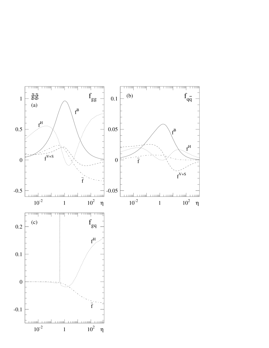
Figure 9: The scaling functions [Eq. (55)] for gluino-pair production from (a) $gg$, (b) $q\bar{q}$, and (c) $gq$ initial states. The (integrable) singularity in (c) is the result of on-shell intermediate squark–gluino states; this singularity is regularized by using a small non-zero squark width. Mass parameters: $m_{\tilde{q}}=280$ GeV, $m_{\tilde{g}}=200$ GeV, and $m_{t}=175$ GeV.

Figure 10: The scaling functions [Eq. (55)] for squark–gluino production from (a) $gq$, (b) $gg$, (c) $q\bar{q}$, and (d) $qq$ initial states. Flavours and chiralities of the squarks are summed over. The (integrable) singularities in (b) and (c) are caused by on-shell intermediate squark–antisquark states, in (d) by on-shell intermediate squark–squark states; these singularities are regularized by using a small non-zero squark width. Mass parameters: $m_{\tilde{q}}=280$ GeV, $m_{\tilde{g}}=200$ GeV, and $m_{t}=175$ GeV.

Noteworthy is the squark-mass dependence of the cross-section for gluino-pair production from quark–antiquark annihilation. This dependence is exemplified in Fig. 11 for the scaling functions, using the mass parameters $m_{\tilde{g}}=200$ GeV, as before, and $m_{\tilde{q}}=175,200,225$ GeV. In the region of almost mass-degenerate squarks and gluinos, the maximum of the LO scaling function $f^{B}$ decreases with increasing squark mass. By contrast, the virtual and soft corrections $f^{V+S}$ increase for small and intermediate energies [$\eta\lesssim 10$], as is also evident from Fig. 9b. The hard-gluon corrections $f^{H}$ are nearly independent. The ratio of the higher-order correction over the lowest-order cross-section will therefore vary rapidly for gluino-pair production in the range where gluino and squark masses are of the same order.

Figure 11: The variation of the scaling functions [Eq. (55)] for $q\bar{q}\to\tilde{g}\tilde{g}$ over a squark-mass interval around $m_{\tilde{q}}=m_{\tilde{g}}$: $m_{\tilde{g}}=200$ GeV and (a) $m_{\tilde{q}}=175$ GeV, (b) $m_{\tilde{q}}=200$ GeV, (c) $m_{\tilde{q}}=225$ GeV.

4.1.2 Threshold Region

The energy region near the production threshold is the base for an important part of the contributions to the hadronic cross-sections. This region is characterized by the small velocity $\beta$ of the produced heavy particles in their centre-of-mass system [$\beta\ll 1$]. Two sources of large corrections can be identified in this threshold region, the leading terms of which can be calculated analytically at NLO. These analytical expressions provide powerful checks of the numerically integrated NLO corrections for arbitrary mass parameters.

First of all, the exchange of (long-range) Coulomb gluons between the slowly moving massive particles in the final state [see Fig. 12a] leads to a singular correction factor $\sim\pi\alpha_{s}/\beta$, which compensates the LO phase-space suppression factor $\beta$ [26]. The scaling function $f^{V+S}$ therefore tends to a non-zero constant at threshold. It should be noted, however, that the screening due to the non-zero lifetimes of the squarks/gluinos reduce this effect considerably.

Figure 12: Generic diagrams leading to (a) the Coulomb singularity, (b) the large threshold logarithms, and (c) the high-energy plateau. The solid external lines represent gluons/(anti)quarks, the dashed ones respresent gluinos/(anti)squarks.

Secondly, as a result of the strong energy dependence of the cross-sections near threshold, large positive “soft” corrections $\sim\log^{i}(\beta^{2})$ ($i=1,2$) are observed in the initial-state gluon-radiation contribution [see Fig. 12b]. They can in fact be resummed [27, 28]. In our analysis we will, however, stick to the strict NLO corrections.

Near threshold the scaling functions can be expanded in $\beta$, leading to the following analytical expressions [suppressing $\Theta(\beta)$]:

Squark–Antisquark:

$$f_{gg}^{B}=\frac{7n_{f}\pi\beta}{192} f_{q\bar{q}}^{B}=\frac{4\pi\beta m_{\tilde{q}}^{2}m_{\tilde{g}}^{2}}{9(m_{\tilde{q}}^{2}+m_{\tilde{g}}^{2})^{2}}$$ (57)

$$f_{gg}^{V+S}=f_{gg}^{B}\frac{11}{336\beta} f_{q\bar{q}}^{V+S}=f_{q\bar{q}}^{B}\frac{7}{48\beta}$$

$$f_{gg}^{H}=f_{gg}^{B}\left[\frac{3}{2\pi^{2}}\log^{2}(8\beta^{2})-\frac{183}{28\pi^{2}}\log(8\beta^{2})\right] f_{q\bar{q}}^{H}=f_{q\bar{q}}^{B}\left[\frac{2}{3\pi^{2}}\log^{2}(8\beta^{2})-\frac{11}{4\pi^{2}}\log(8\beta^{2})\right]$$

$$\bar{f}_{gg}=-f_{gg}^{B}\frac{3}{2\pi^{2}}\log(8\beta^{2}) \bar{f}_{q\bar{q}}=-f_{q\bar{q}}^{B}\frac{2}{3\pi^{2}}\log(8\beta^{2}).$$

For squark–antisquark final states the scaling functions for equal and different flavours are identical ($f_{q^{\prime}\bar{q}}=f_{q\bar{q}}$) near threshold.

Squark–Squark:

$$f_{qq}^{B}=\frac{8\pi\beta m_{\tilde{q}}^{2}m_{\tilde{g}}^{2}}{27(m_{\tilde{q}}^{2}+m_{\tilde{g}}^{2})^{2}} f_{q^{\prime}q}^{B}=\frac{4\pi\beta m_{\tilde{q}}^{2}m_{\tilde{g}}^{2}}{9(m_{\tilde{q}}^{2}+m_{\tilde{g}}^{2})^{2}}$$ (59)

$$f_{qq}^{V+S}=f_{qq}^{B}\frac{1}{24\beta} f_{q^{\prime}q}^{V+S}=f_{q^{\prime}q}^{B}\frac{1}{24\beta}$$

$$f_{qq}^{H}=f_{qq}^{B}\left[\frac{2}{3\pi^{2}}\log^{2}(8\beta^{2})-\frac{7}{2\pi^{2}}\log(8\beta^{2})\right] f_{q^{\prime}q}^{H}=f_{q^{\prime}q}^{B}\left[\frac{2}{3\pi^{2}}\log^{2}(8\beta^{2})-\frac{19}{6\pi^{2}}\log(8\beta^{2})\right]$$

$$\bar{f}_{qq}=-f_{qq}^{B}\frac{2}{3\pi^{2}}\log(8\beta^{2}) \bar{f}_{q^{\prime}q}=-f_{q^{\prime}q}^{B}\frac{2}{3\pi^{2}}\log(8\beta^{2}).$$

Gluino–Gluino:

$$f_{gg}^{B}=\frac{27\pi\beta}{64} f_{q\bar{q}}^{B}=\frac{\pi\beta}{3}\left(\frac{m_{\tilde{g}}^{2}-m_{\tilde{q}}^{2}}{m_{\tilde{q}}^{2}+m_{\tilde{g}}^{2}}\right)^{2}$$ (61)

$$f_{gg}^{V+S}=f_{gg}^{B}\frac{1}{16\beta} f_{q\bar{q}}^{V+S}=f_{q\bar{q}}^{B}\frac{3}{16\beta}$$

$$f_{gg}^{H}=f_{gg}^{B}\left[\frac{3}{2\pi^{2}}\log^{2}(8\beta^{2})-\frac{29}{4\pi^{2}}\log(8\beta^{2})\right] f_{q\bar{q}}^{H}=f_{q\bar{q}}^{B}\left[\frac{2}{3\pi^{2}}\log^{2}(8\beta^{2})-\frac{41}{12\pi^{2}}\log(8\beta^{2})\right]$$

$$\bar{f}_{gg}=-f_{gg}^{B}\frac{3}{2\pi^{2}}\log(8\beta^{2}) \bar{f}_{q\bar{q}}=-f_{q\bar{q}}^{B}\frac{2}{3\pi^{2}}\log(8\beta^{2}).$$

The LO and NLO threshold cross-sections for gluino-pair production from quark–antiquark annihilation vanish if the squarks and gluinos are mass degenerate. This follows from the destructive interference between the three LO diagrams. In Fig. 11 this phenomenon is clearly visible.

Squark–Gluino:

$$f_{qg}^{B}=\frac{\pi\beta}{(m_{\tilde{q}}+m_{\tilde{g}})^{3}}\left\{\frac{2}{9}m_{\tilde{q}}m_{\tilde{g}}^{2}+\frac{1}{2}m_{\tilde{q}}^{2}m_{\tilde{g}}+\frac{1}{2}m_{\tilde{q}}^{3}\right\}$$ (63)

$$f_{qg}^{V+S}=\frac{\pi}{(m_{\tilde{q}}+m_{\tilde{g}})^{3}}\left\{-\frac{1}{192}m_{\tilde{q}}m_{\tilde{g}}^{2}+\frac{3}{64}m_{\tilde{q}}^{3}\right\}$$

$$f_{qg}^{H}=\frac{f_{qg}^{B}}{\pi^{2}}\left\{\frac{13}{12}\log^{2}(8\beta^{2})+\frac{13}{6}\log(8\beta^{2})\log\left(\frac{4m_{\tilde{q}}m_{\tilde{g}}}{(m_{\tilde{q}}+m_{\tilde{g}})^{2}}\right)\right\}$$

$$\qquad+\frac{\beta}{\pi(m_{\tilde{q}}+m_{\tilde{g}})^{3}}\log(8\beta^{2})\left\{-\frac{529}{432}m_{\tilde{q}}m_{\tilde{g}}^{2}-\frac{65}{24}m_{\tilde{q}}^{2}m_{\tilde{g}}-\frac{121}{48}m_{\tilde{q}}^{3}\right\}$$

$$\bar{f}_{qg}=-f_{qg}^{B}\frac{13}{12\pi^{2}}\log(8\beta^{2})\qquad\beta=\sqrt{1-\frac{4m_{\tilde{q}}m_{\tilde{g}}}{s-(m_{\tilde{q}}-m_{\tilde{g}})^{2}}}~{}.$$

Note that for squark–gluino production the leading corrections factorize only partly in terms of the LO cross-section. This in contrast to the other production processes, which involve equal-mass final-state particles.

4.1.3 High-Energy Region

At high energies the NLO partonic cross-sections can asymptotically approach a non-zero constant, rather than scaling with $1/s$ as the LO cross-sections:

$$\hat{\sigma} \sim\frac{\alpha_{s}^{2}}{s}$$ (LO) (64)

$$\hat{\sigma} \sim\frac{\alpha_{s}^{3}}{m^{2}} \text{(NLO)}.$$ (65)

This is caused by almost on-shell, soft gluons in space-like propagators, associated with hard-gluon/quark radiation [see Fig. 12c]. Since the splitting probabilities $q\to qg$ and $g\to gg$ are scale-invariant mod. logarithms, the size of the NLO cross-section is set by the centre-of-mass energy of the subprocess induced by the virtual gluon (marked “Born” in Fig. 12c). For the dominant contributions this centre-of-mass energy is of the order of the squark/gluino masses, i.e. not far above the threshold. It should be noted that these high-energy plateaus only have a marginal influence on the hadronic cross-sections, as the main part of the contributions originates from the partonic energy region near the production threshold.

Exploiting the factorization in the transverse gluon momentum at high energies [29], the high-energy scaling functions can be determined analytically.

Squark–Antisquark:

$$f_{gg}^{H} = \frac{2159}{4320\pi} \qquad f_{gq}^{H} = \frac{2159}{19440\pi}$$ (67)

$$\bar{f}_{gg} = -\frac{11}{72\pi} \qquad\bar{f}_{gq} = -\frac{11}{324\pi}.$$

The ratio of the $f_{gg}$ and $f_{gq}$ scaling functions is given by $2N:C_{F}=9:2$. This ratio corresponds to the probability of emitting a soft gluon from a gluon [$\sim N$, 2 sources] or a quark ($\sim C_{F}$, 1 source).

Squark–Squark:

The squark-pair production cross-section does not exhibit a high-energy plateau, since no space-like gluon-exchange diagrams are possible at NLO.

Gluino–Gluino:

$$f_{gg}^{H} = \frac{1949}{800\pi} \qquad f_{gq}^{H} = \frac{1949}{3600\pi}$$ (69)

$$\bar{f}_{gg} = -\frac{177}{160\pi} \qquad\bar{f}_{gq} = -\frac{59}{240\pi}.$$

The ratio of the $f_{gg}$ and $f_{gq}$ scaling functions is given again by $2N:C_{F}=9:2$.

Squark–Gluino:

$$f_{qg}^{H} = \frac{517}{864\pi} f_{q\bar{q}}^{H}= f_{q^{\prime}\bar{q}}^{H} = \frac{517}{1944\pi} f_{qq}^{H}= f_{q^{\prime}q}^{H} =\frac{517}{972\pi}$$ (71)

$$\bar{f}_{qg} = -\frac{5}{18\pi} \bar{f}_{q\bar{q}}= \bar{f}_{q^{\prime}\bar{q}} = -\frac{10}{81\pi} \bar{f}_{qq}= \bar{f}_{q^{\prime}q} =-\frac{20}{81\pi}.$$

These (simple) high-energy limits are derived for equal squark and gluino masses; the results for arbitrary masses are very complicated and are therefore not given explicitly. The ratio of the $f_{qg}$, $f_{q\bar{q}}$, and $f_{qq}$ scaling functions is given by $N:C_{F}:2C_{F}=9:4:8$, irrespective of the precise values for the squark and gluino masses.

4.2 Hadronic Cross-Sections

Finally we discuss in this subsection the hadronic cross-sections for the production of squarks and gluinos. The analyses are performed for the Fermilab $p\bar{p}$ collider Tevatron with a centre-of-mass energy of $\sqrt{S}=1.8$ TeV, and for the CERN $pp$ collider LHC with a centre-of-mass energy of $\sqrt{S}=14$ TeV. In analogy to the experimental analyses, we consider the following four hadronic production processes

$$p\bar{p}/pp \rightarrow \tilde{q}\bar{\tilde{q}}$$ (72)

$$p\bar{p}/pp \rightarrow \tilde{q}\tilde{q},\bar{\tilde{q}}\bar{\tilde{q}}$$ (73)

$$p\bar{p}/pp \rightarrow \tilde{g}\tilde{g}$$ (74)

$$p\bar{p}/pp \rightarrow \tilde{q}\tilde{g},\bar{\tilde{q}}\tilde{g}.$$ (75)

As before the chiralities and flavours of the squarks (e.g. $\tilde{u}_{L},\tilde{d}_{R}$) are implicitly summed over. Yet stop production is not taken into account; these final states will be analyzed in a forthcoming report [9]. The charge-conjugate final states are now properly taken into account in the reactions (73) and (75). From now on we will refer to these two hadronic reactions, for simplicity, as $\tilde{q}\tilde{q}$ (squark–squark) and $\tilde{q}\tilde{g}$ (squark–gluino) production, respectively.

Various aspects of the above reactions will be presented in detail. First of all, the dependence of the cross-sections on the renormalization/factorization scale and parton densities is investigated. Then the NLO corrections are studied for a default choice of scale and parton densities. We discuss the NLO effects on the differential distributions with respect to the rapidity $y$ and transverse momentum $p_{t}$ of one of the outgoing particles. Finally we describe the NLO effects on the total cross-sections and their implications on the experimental search for squarks and gluinos.

4.2.1 Scale and Parton-Density Dependence

The total hadronic cross-sections are obtained by convoluting the partonic cross-sections with the relevant parton densities [in the proton or antiproton]:

$$\sigma(S,Q^{2})=\sum_{i,j=g,q,\bar{q}}\int_{\tau}^{1}dx_{1}\int_{\tau/x_{1}}^{1}dx_{2}\,f_{i}^{h_{1}}(x_{1},Q^{2})\,f_{j}^{h_{2}}(x_{2},Q^{2})\,\hat{\sigma}_{ij}(x_{1}x_{2}S,Q^{2})\Big{|}_{\tau=4m^{2}/S}$$ (76)

The partons $i$ and $j$ carry fractions $x_{1}$ and $x_{2}$ of the original momenta of the hadrons $h_{1}$ ($=p$) and $h_{2}$ ($=\bar{p}/p$), respectively. The integrations in Eq. (76) are performed numerically, using the Monte Carlo integration routine VEGAS [30]. The parton densities $f_{i}^{h}$ have been extracted from a large variety of experiments and are available in various parametrizations. To estimate the associated uncertainty, we compare the results for a sample of three different parametrizations.

As a first step, we present for reactions (72)–(75) the dependence of the total cross-section on the renormalization and factorization scale $Q=Q_{R}=Q_{F}$ in Figs. 13 and 14. We have checked that the separate variation of the factorization scale $Q_{F}$ and the renormalization scale $Q_{R}$ leads to a variation of the next-to-leading order cross-section (roughly) within the band generated by $Q$. We can therefore keep the discussion to this simplified case without loss of generality. The scale is restricted to $Q\lesssim 1$ TeV, as the parton densities are not available beyond this value.

The results for the Tevatron are given in Fig. 13, using the mass parameters $m_{\tilde{q}}=280$ GeV, $m_{\tilde{g}}=200$ GeV, and $m_{t}=175$ GeV. For a consistent comparison of LO and NLO results, we calculate all quantities [$\alpha_{s}(Q_{R}^{2})$, the parton densities, and the partonic cross-sections] in LO and NLO, respectively. In LO we use the parton densities of GRV94 [20] and CTEQ3 [32] with the corresponding QCD couplings. At NLO this is compared with the parton densities of GRV94 [20], CTEQ3 [32], and MRS(A’) [33]. In LO the scale dependence is steep and monotonic. Changing the scale from $Q=2m$ to $Q=m/2$, the cross-section increases by 100–120%. In NLO the scale dependence is strongly reduced, to about 40–50% in this interval. At the same time the cross-section is significantly enhanced at the central scale ($Q=m$). The uncertainty originating from the various parametrizations of the parton densities in NLO amounts to $\lesssim 10\%$ at the central scale. An exception is the squark–squark cross-section, which is dependent on the badly determined sea-quark distribution.

The results for the LHC are given in Fig. 14, using the mass parameters $m_{\tilde{q}}=600$ GeV, $m_{\tilde{g}}=500$ GeV, and $m_{t}=175$ GeV. Here, too, a strong reduction of the scale dependence is observed by taking into account the NLO corrections, as well as a clear enhancement of the cross-section at the central scale. In the interval between $Q=m$ and $Q=m/2$ the LO cross-section increases by about 35%, whereas the variation for the NLO results is reduced to only 5–10%. At the LHC the dependence on the factorization scale is very weak and the residual scale dependence is dominated by $\alpha_{s}$ [in contrast with the Tevatron where fairly large $x$ values in the parton distributions give rise to a stronger factorization-scale dependence]. The uncertainty due to different parametrizations of the parton densities in NLO amounts to $\lesssim 13\%$ at the central scale. This is a result of the prominent role played by the gluon densities at the LHC.

In conclusion, for all four reactions and for both hadron colliders the scale dependence is reduced by a factor of 2.5–4 when the theoretical predictions are improved by taking into account the next-to-leading order SUSY-QCD corrections. Even a broad and shallow maximum develops at scales near one third of the central scale. In the following we will adopt GRV94 parton densities and take $Q=m$ as the default scale; this results in a conservative estimate of the cross-sections.

Figure 13: The dependence on the renormalization/factorization scale $Q$ of the LO and NLO cross-sections for (a) squark–antisquark, (b) squark–squark, (c) gluino–gluino, and (d) squark–gluino production at the Tevatron ($\sqrt{S}=1.8$ TeV). Parton densities: GRV94 (solid), CTEQ3 (dashed), and MRS(A’) (dotted). Mass parameters: $m_{\tilde{q}}=280$ GeV, $m_{\tilde{g}}=200$ GeV, and $m_{t}=175$ GeV.

Figure 14: The dependence on the renormalization/factorization scale $Q$ of the LO and NLO cross-sections for (a) squark–antisquark, (b) squark–squark, (c) gluino–gluino, and (d) squark–gluino production at the LHC ($\sqrt{S}=14$ TeV). Parton densities: GRV94 (solid), CTEQ3 (dashed), and MRS(A’) (dotted). Mass parameters: $m_{\tilde{q}}=600$ GeV, $m_{\tilde{g}}=500$ GeV, and $m_{t}=175$ GeV.

4.2.2 Differential Distributions: Transverse Momentum and Rapidity

The hadronic differential distributions are obtained by convoluting the partonic double-differential distributions with the relevant parton densities. We consider the distributions with respect to the transverse momentum $p_{t}$ and rapidity $y$ of one of the outgoing squarks/gluinos. The corresponding double-differential hadronic distribution is given by

$$\frac{d^{2}\sigma}{dp_{t}dy}=2p_{t}S\sum_{i,j=g,q,\bar{q}}\int_{x_{1}^{-}}^{1}dx_{1}\int_{x_{2}^{-}}^{1}dx_{2}\,x_{1}f_{i}^{h_{1}}(x_{1},Q^{2})\,x_{2}f_{j}^{h_{2}}(x_{2},Q^{2})\,\frac{d^{2}\hat{\sigma}_{ij}(x_{1}x_{2}S,Q^{2})}{dt\,du}.$$ (77)

The definitions of $p_{t}$ and $y$ and of the integration boundaries can be found in Appendix B. Squarks and antisquarks are not distinguished in the final state. So, for $\tilde{q}\bar{\tilde{q}}$, $\tilde{q}\tilde{q}$, and $\tilde{g}\tilde{g}$ final states we have to add the distributions with respect to both final-state particles. The rapidity distributions, as presented in Figs. 16 and 18, are defined as the sum of the contributions of positive and negative rapidity. The distributions are normalized to unity.

In Fig. 15 the normalized $p_{t}$ distribution is given for the Tevatron. The input mass parameters are $m_{\tilde{q}}=280$ GeV, $m_{\tilde{g}}=200$ GeV, and $m_{t}=175$ GeV. For the scale $Q$ and for the parton densities we take the default settings [$Q=m$ and GRV94]. In order to perform a consistent comparison of LO and NLO results, the parton densities are used with the associated values for $\alpha_{s}$. In Fig. 16 the normalized $y$ distribution is shown. The corresponding distributions for the LHC can be found in Figs. 17 and 18, elaborated for $m_{\tilde{q}}=600$ GeV, $m_{\tilde{g}}=500$ GeV, and $m_{t}=175$ GeV.

The normalized $p_{t}$ distributions are hardly affected by the transition from LO to NLO. In total, the NLO corrections render the distributions a little softer. This is caused by the fact that for high-energetic massive particles the probability of losing energy through radiation is large. The normalized rapidity spectra in LO and NLO are identical for all practical purposes.

In conclusion, the properly normalized distributions of the squarks and gluinos in transverse momentum and rapidity are described quite well by the lowest-order approximation.

Figure 15: Normalized transverse-momentum distributions in LO (dotted) and NLO (solid) at the Tevatron ($\sqrt{S}=1.8$ TeV). Parton densities: GRV94, with scale $Q=m$; mass parameters: $m_{\tilde{q}}=280$ GeV, $m_{\tilde{g}}=200$ GeV, and $m_{t}=175$ GeV.

Figure 16: Normalized rapidity distributions in LO (dotted) and NLO (solid) at the Tevatron ($\sqrt{S}=1.8$ TeV). Parton densities: GRV94, with scale $Q=m$; mass parameters: $m_{\tilde{q}}=280$ GeV, $m_{\tilde{g}}=200$ GeV, and $m_{t}=175$ GeV.

Figure 17: Normalized transverse-momentum distributions in LO (dotted) and NLO (solid) at the LHC ($\sqrt{S}=14$ TeV). Parton densities: GRV94, with scale $Q=m$; mass parameters: $m_{\tilde{q}}=600$ GeV, $m_{\tilde{g}}=500$ GeV, and $m_{t}=175$ GeV.

Figure 18: Normalized rapidity distributions in LO (dotted) and NLO (solid) at the LHC ($\sqrt{S}=14$ TeV). Parton densities: GRV94, with scale $Q=m$; mass parameters: $m_{\tilde{q}}=600$ GeV, $m_{\tilde{g}}=500$ GeV, and $m_{t}=175$ GeV.

4.2.3 Total Cross-Sections for Squark and Gluino Production

$K$-factors:

To facilitate the quantitative comparison of LO and NLO cross-sections we define the ratio

$$K=\sigma_{NLO}/\sigma_{LO},$$ (78)

usually referred to as the $K$-factor. For consistency, the cross-section $\sigma_{LO}$ ($\sigma_{NLO}$) is calculated for all entries taken at leading (next-to-leading) order, i.e. couplings, parton densities, and parton cross-sections.

In Fig. 19 we present the $K$-factors at the Tevatron for the reactions (72)–(75). For the scale $Q$ and the parton densities we take the default settings [$Q=m$ and GRV94]. In Fig. 19a the $K$-factors are displayed for a gluino mass $m_{\tilde{g}}=200$ GeV and for squark masses in the range 150–400 GeV, whereas in Fig. 19b the role of the squarks and gluinos is interchanged. The corrections strongly depend on the process. With the exception of the squark-pair production process, which is rather unimportant at the Tevatron, all processes are subject to large, positive corrections between $+10\%$ and $+90\%$. The $K$-factors for squark final states are almost mass-independent. By contrast, the $K$-factors for the (dominant) final states that involve at least one gluino exhibit a strong mass dependence. The particularly strong mass dependence of the gluino-pair $K$-factors for almost mass-degenerate squarks and gluinos is a direct consequence of the phenomena described in Section 4.1.1 for the scaling functions, since a large part of the hadronic cross-section originates from the quark–antiquark channel. For a fixed gluino mass and increasing squark masses the LO cross-section decreases, whereas the virtual corrections increase. This leads to the observed increase of the $K$-factor. If the squark mass is kept fixed and the gluino mass is increased, the reverse is observed.

In Fig. 20 the $K$-factors are presented for the LHC. The input is the same as before, except for the fact that we consider fixed ratios of the squark and gluino masses: $m_{\tilde{q}}/m_{\tilde{g}}=0.8,1.2,1.6\,\text{and}\,2$ [Figs. 20 a – d ]. Again, the corrections are positive and in general large, between $+5\%$ and $+90\%$. The mass dependence and the absolute size of the $K$-factors for squark final states are moderate. By contrast, for final states involving gluinos the corrections are substantially larger and exhibit a strong mass dependence. The influence of the squark mass on the gluino-pair cross-section is less pronounced than for the Tevatron, since the gluon–gluon initial state yields the dominant contributions.

Figure 19: The $K$-factors [Eq. (78)] for the Tevatron ($\sqrt{S}=1.8$ TeV). Parton densities: GRV94, with scale $Q=m$; mass parameters: $m_{t}=175$ GeV and (a) $m_{\tilde{g}}=200$ GeV, (b) $m_{\tilde{q}}=200$ GeV.

Figure 20: The $K$-factors [Eq. (78)] for the LHC ($\sqrt{S}=14$ TeV). Parton densities: GRV94, with scale $Q=m$; top-quark mass: $m_{t}=175$ GeV.

Total cross-sections:

The absolute size of the total hadronic cross-sections plays a crucial role in the experimental analyses. As long as no squarks and gluinos are discovered, the exclusion limits of the masses are derived by comparing the experimental data with the expected rates based on the theoretical predictions of the cross-sections. If squarks and gluinos are discovered, the masses of the particles will be determined experimentally by the same method.

In Fig. 21 the total cross-sections are given for the Tevatron. The NLO results are based on the default settings: renormalization/factorization scale $Q=m$ and GRV94 parton densities. These cross-sections are compared with the LO parametrizations adopted in the experimental analyses [11, 12] until recently [EHLQ parton densities, with $Q$ equal to the partonic centre-of-mass energy]. Over the full mass range covered by the Tevatron, the net effect of the NLO corrections is to raise the derived lower mass bounds by $+10$ GeV to $+30$ GeV.

In Fig. 22 the total cross-sections are given for the LHC, using the default settings and a representative range of squark and gluino masses. Over the full mass range covered by the LHC, the cross-sections are increased by the NLO corrections, leading to a shift in the associated particle masses in the range between $+10$ GeV and $+50$ GeV.

Figure 21: The total cross-section for the Tevatron ($\sqrt{S}=1.8$ TeV). NLO (solid): GRV94 parton densities, with scale $Q=m$; compared with LO (dashed): EHLQ parton densities, at the scale $Q=\sqrt{s}$.

Figure 22: The total cross-section for the LHC ($\sqrt{S}=14$ TeV). NLO (solid) compared with LO (dotted). Parton densities: GRV94, with scale $Q=m$.

4.2.4 Implications for Experimental Searches

The precise knowledge of the cross-sections at next-to-leading order SUSY-QCD has a profound impact on the experimental analyses:

(i) The renormalization/factorization scale dependence is reduced by roughly a factor of 2.5–4 compared with leading-order calculations, and the theoretical predictions of the cross-sections are stable. Taking for the renormalization/factorization scale $Q$ the average mass $m$ of the produced particles results in a conservative estimate for the cross-sections at NLO.

(ii) The NLO corrections are large and positive at the central scale $Q=m$. The NLO corrections must therefore be included in the analyses to obtain adequate theoretical predictions for the total cross-sections, as required for deriving experimental mass bounds or measuring the squark and gluino masses.

(iii) The shape of the differential distributions in transverse momentum and rapidity of one of the outgoing squarks or gluinos is hardly affected by the NLO corrections.

(iv) The NLO cross-sections raise the present lower mass bounds for squarks and gluinos derived from Tevatron data by $+10$ GeV to $+30$ GeV.

5 Conclusions and Outlook

In this report we have presented the next-to-leading order SUSY-QCD corrections for the production cross-sections of squarks and gluinos at the hadron colliders Tevatron and LHC. By reducing the scale dependence of the cross-sections considerably, the quality of the theoretical predictions is substantially improved compared with the lowest-order calculations. The NLO cross-sections provide a solid basis for experimental analyses of squark and gluino mass bounds/measurements at hadron colliders.

So far the calculations have been performed for mass-degenerate squarks associated with the five light quark flavours. Generally, small mass differences between the $L$ and $R$ squark states for a given flavour are suggested by supergravity-inspired parametrizations of low-energy supersymmetry. Due to the large top–Higgs Yukawa coupling, however, the assumption of mass degeneracy is expected to be strongly broken for the two stop states $\tilde{t}_{1}$ and $\tilde{t}_{2}$, mixtures of the $L$ and $R$ chirality states $\tilde{t}_{L}$ and $\tilde{t}_{R}$. In these cases the NLO SUSY-QCD cross-sections require the extension of the theoretical analysis to different left- and right-handed couplings of the quarks to squarks and gluinos, adding to the complexity of the calculation in a non-trivial way. For final-state stop particles this analysis is in progress and will be completed in due time.

Note

The Fortran codes of the NLO cross-sections can be obtained from hoepker @@ x4u2.desy.de, spira @@ cern.ch, or wimb @@ lorentz.leidenuniv.nl.

Appendix A Fermion-Flow Diagrams in SUSY-QCD

The field-theoretic components of supersymmetric QCD are quarks/squarks and gluons/gluinos. The Majorana character of gluinos renders the evaluation of Feynman diagrams involving these particles somewhat cumbersome. However, a simple prescription has recently been proposed in Ref. [34], which allows an easy and fail-safe evaluation of the diagrams. It involves the definition of a continuous fermion-flow line, which in general does not coincide with the flow of the fermion number [given by the direction of the Dirac propagator line]. The amplitude must be evaluated along the fermion-flow according to the standard rules. In this way also fermion-number-violating processes like $qq\to\tilde{q}\tilde{q}$ can be described in a straightforward fashion.

This method is equivalent to the usual evaluation of SUSY-QCD diagrams if the analytic form of the propagators and vertices involving fermions is adjusted properly. The analytic expressions associated with these propagators and vertices are given explicitly in Fig. 23. Indices of the fundamental/adjoint representation of colour $SU(3)$ are denoted by $i,j$/$a$–$c$, the generators of the fundamental representation by $t^{a}=\lambda^{a}/2\,\ (a=1,...,8)$, and the structure constants by $f^{abc}$. The index $\mu$ is a Lorentz index, $\alpha$ and $\beta$ are Dirac indices. The coupling constants $g_{s}$ and $\hat{g}_{s}$ are the gauge and Yukawa couplings, respectively. The fermion-flow is defined in the diagrams by an additional directed line, parallel to the propagators. All other SUSY-QCD vertices and propagators are not affected by defining the fermion-flow lines. The flavour of the quarks and squarks are conserved in the SUSY-QCD interactions.

Figure 23: Analytic expressions for the SUSY-QCD propagators and vertices that involve a specific fermion-flow, defined by the line parallel to the propagators.

Appendix B Kinematics and Phase Space

The kinematics and phase space for the production processes of a pair of squarks or a pair of gluinos are the same as for top–antitop production [17]. However, for the production of squark–gluino final states, the masses of the heavy particles are different. The kinematical and phase-space relations must therefore be derived for this more general case. Identifying squark and gluinos masses, we recover the formulae for squark and gluino pairs.

B.1 Partonic Processes

We shall discuss the partonic process

$$q(k_{1})+g(k_{2})\longrightarrow\tilde{q}(p_{1})+\tilde{g}(p_{2})\,\,\left[+g(k_{3})\right]$$ (79)

for illustration. All particles are on shell, i.e. $k_{1}^{2}=k_{2}^{2}=0$, $p_{1}^{2}=m_{\tilde{q}}^{2}$, $p_{2}^{2}=m_{\tilde{g}}^{2}$ and $k_{3}^{2}=0$. The kinematics of the radiative process is characterized by the invariant variables introduced in Eq. (29); they are related by energy–momentum conservation:

$$s_{4} =s+t_{g}+u_{1}\qquad\qquad\qquad s_{3} =s+u_{6}+u_{7}$$

$$s_{5} =s+t^{\prime}+u^{\prime}\qquad\qquad\qquad u_{6} =-s-t_{g}-t^{\prime}$$

$$u_{7} =-s-u_{g}-u^{\prime}.$$

The total partonic cross-section is obtained by integrating the double-differential cross-section

$$\hat{\sigma} = \int_{t_{g}^{-}}^{t_{g}^{+}}dt_{g}\int_{0}^{s_{4}^{max}(t_{g})}ds_{4}\,\frac{d^{2}\hat{\sigma}}{dt_{g}\,ds_{4}}$$ (80)

within the limits

$$t_{g}^{\pm} = {}-\frac{s+m_{\tilde{g}}^{2}-m_{\tilde{q}}^{2}}{2}\pm\frac{1}{2}\sqrt{(s-m_{\tilde{g}}^{2}-m_{\tilde{q}}^{2})^{2}-4m_{\tilde{g}}^{2}m_{\tilde{q}}^{2}}$$

$$s_{4}^{max}(t_{g}) = s+t_{g}+m_{\tilde{g}}^{2}-m_{\tilde{q}}^{2}+\frac{m_{\tilde{g}}^{2}s}{t_{g}}.$$

The invariant energy of the $\tilde{q}g$ subsystem in the final state is characterized by the variable $s_{4}$, the square of the momentum transfer from the gluon (quark) in the initial state to the gluino in the final state by $t=t_{g}+m_{\tilde{g}}^{2}$  ($u=u_{g}+m_{\tilde{g}}^{2}$).

The double-differential cross-section in Eq. (80) can be derived by integrating the general four-fold differential cross-section over the angles $\theta_{i}$ defined in the centre-of-mass frame of the $\tilde{q}g$ subsystem. In this particular frame the $n$-dimensional momenta are given by

$$k_{1} = (w_{1},0,...,0,0,|p|\sin\psi,|p|\cos\psi-w_{2})$$ (81)

$$k_{2} = (w_{2},0,...,0,0,0,w_{2})$$

$$k_{3} = (w_{3},0,...,0,w_{3}\sin\theta_{1}\sin\theta_{2},w_{3}\sin\theta_{1}\cos\theta_{2},w_{3}\cos\theta_{1})$$

$$p_{1} = (E_{1},0,...,0,-w_{3}\sin\theta_{1}\sin\theta_{2},-w_{3}\sin\theta_{1}\cos\theta_{2},-w_{3}\cos\theta_{1})$$

$$p_{2} = (E_{2},0,...,0,0,|p|\sin\psi,|p|\cos\psi).$$

The energies $w_{i},E_{i}$, the momentum $|p|$, and the angle $\psi$ are related to the $\theta_{i}$-independent invariants $s,\,t_{g},\,u_{g}$, and $s_{4}$ introduced earlier:

$$w_{1} =\frac{s+u_{g}}{2\sqrt{s_{4}+m_{\tilde{q}}^{2}}} \qquad w_{2} =\frac{s+t_{g}}{2\sqrt{s_{4}+m_{\tilde{q}}^{2}}} \qquad w_{3} =\frac{s_{4}}{2\sqrt{s_{4}+m_{\tilde{q}}^{2}}}$$

$$E_{1} =\frac{s_{4}+2m_{\tilde{q}}^{2}}{2\sqrt{s_{4}+m_{\tilde{q}}^{2}}} \qquad E_{2} ={}-\frac{t_{g}+u_{g}+2m_{\tilde{g}}^{2}}{2\sqrt{s_{4}+m_{\tilde{q}}^{2}}}$$ (83)

$$|p| =\frac{\sqrt{(t_{g}+u_{g})^{2}-4m_{\tilde{g}}^{2}s}}{2\sqrt{s_{4}+m_{\tilde{q}}^{2}}} \qquad\cos\psi =\frac{t_{g}s_{4g}-s(u_{g}+2m_{\tilde{g}}^{2})}{(s+t_{g})\sqrt{(t_{g}+u_{g})^{2}-4m_{\tilde{g}}^{2}s}}.$$

Using these relations, all the invariant variables defined in Eq. (29) can be expressed in terms of $s,t_{g},u_{g},s_{4},\theta_{i}$. For certain combinations of invariants, it is convenient to define the $z$-axis with respect to $k_{1}$ or $p_{2}$ (instead of $k_{2}$). Writing the $n$-dimensional angular part of the phase-space element as $d\Omega_{n}=\sin^{1-2\varepsilon}(\theta_{1})\,d\theta_{1}\,\sin^{-2\varepsilon}(\theta_{2})\,d\theta_{2}$, the double-differential cross-section is obtained from the matrix element ${\cal M}^{R}$ in the following way:

$$s^{2}\,\frac{d^{2}\sigma^{R}}{dt_{g}\,ds_{4}} = K_{ij}\,\frac{S_{\varepsilon}^{2}\mu^{2\varepsilon}}{2\Gamma(1-2\varepsilon)}\left[\frac{t_{g}u_{g}-m_{\tilde{g}}^{2}s}{\mu^{2}s}\right]^{-\varepsilon}\Theta(t_{g}u_{g}-m_{\tilde{g}}^{2}s)\,\Theta(s-[m_{\tilde{q}}+m_{\tilde{g}}]^{2})$$ (84)

$$\times\,\frac{(s_{4})^{1-2\varepsilon}}{(s_{4}+m_{\tilde{q}}^{2})^{1-\varepsilon}}\,\Theta(s_{4})\int d\Omega_{n}\sum|{\cal M}^{R}|^{2}.\qquad$$

In the limit $m_{\tilde{q}}=m_{\tilde{g}}$ the well-known expressions of Ref. [17] are recovered for the equal-mass case. The $\Theta$-functions represent the requirements of positive energies and $\cos^{2}\psi\leq 1$. They translate into the integration boundaries of the $s_{4}$ and $t_{g}$ integrals in Eq.(80).

As described in Section 3.3.2, on-shell resonance production of intermediate particles is possible. For squark–gluino production, this must be analyzed carefully in the kinematical range where the three-particle final state $\tilde{g}\tilde{q}\bar{q}$ approaches the two-particle final state $\tilde{g}\tilde{g}$ (if $m_{\tilde{g}}>m_{\tilde{q}}$) or $\tilde{q}\bar{\tilde{q}}$ (if $m_{\tilde{q}}>m_{\tilde{g}}$). This gives rise to singularities in $1/s_{3}$ or $1/s_{4g}$, as is evident from Fig. 24, if the momentum flow approaches the $\tilde{q}$ or $\tilde{g}$ mass shells.

Figure 24: Examples for on-shell intermediate resonance states: (a) gluino-pair intermediate state for squark–gluino final states; (b) squark–antisquark intermediate state for squark–gluino final states; and (c) squark–gluino intermediate state for gluino-pair final states.

After exchanging the order of the integrations, the total cross-section corresponding to the diagram in Fig. 24a can be written as

$$\hat{\sigma}=\int_{0}^{s_{4}^{+}}ds_{4}\int_{t_{g}^{-}(s_{4})}^{t_{g}^{+}(s_{4})}dt_{g}\,\frac{d^{2}\hat{\sigma}}{dt_{g}\,ds_{4}}\equiv\int_{0}^{s_{4}^{+}}ds_{4}\,\frac{f(s_{4g})}{s_{4g}^{2}}$$ (85)

$$s_{4}^{+}=s+m_{\tilde{g}}^{2}-m_{\tilde{q}}^{2}-2\sqrt{sm_{\tilde{g}}^{2}}\qquad t_{g}^{\pm}(s_{4})={}-\frac{s-s_{4g}}{2}\pm\frac{1}{2}\sqrt{(s-s_{4g})^{2}-4sm_{\tilde{g}}^{2}}.$$

The singularity in $s_{4g}$ for $m_{\tilde{g}}>m_{\tilde{q}}$ can be regularized by inserting the non-zero gluino width and introducing the Breit–Wigner form, i.e. $1/[s_{4g}^{2}+m_{\tilde{g}}^{2}\Gamma_{\tilde{g}}^{2}]$, for the (absolute) square of the propagator.

Inserting the identity $f(s_{4g})=[f(s_{4g})-f(0)]+f(0)$, the part of the cross-section related to $f(0)$ corresponds to the (LO) production of an on-shell intermediate gluino and subsequent (LO) decay of this gluino into a squark and antiquark, since

$$f(0)=\hat{\sigma}^{B}_{\tilde{g}\tilde{g}}\,\frac{m_{\tilde{g}}\Gamma_{\tilde{g}}}{\pi}\,\frac{\Gamma^{B}_{\tilde{g}\to\tilde{q}}}{\Gamma_{\tilde{g}}}$$

and $m_{\tilde{g}}\Gamma_{\tilde{g}}/[s_{4g}^{2}+m_{\tilde{g}}^{2}\Gamma_{\tilde{g}}^{2}]\to\pi\delta(s_{4g})$ for small $\Gamma_{\tilde{g}}$. This part is already accounted for by the lowest-order $\tilde{g}\tilde{g}$ cross-section and has to be subtracted from the $\tilde{g}\tilde{q}\bar{q}$ cross-section. After the formal expansion of $f(s_{4g})$ around $s_{4g}=0$, the remaining part

$$\Delta\hat{\sigma}=\int_{0}^{s_{4}^{+}}ds_{4}\,\frac{f(s_{4g})-f(0)}{s_{4g}^{2}+m_{\tilde{g}}^{2}\Gamma_{\tilde{g}}^{2}}$$ (86)

is finite and well defined as a principal-value integral, since $s_{4g}/[s_{4g}^{2}+m_{\tilde{g}}^{2}\Gamma_{\tilde{g}}^{2}]\to{\cal P}(1/s_{4g})$ for small $\Gamma_{\tilde{g}}$.

For $m_{\tilde{q}}>m_{\tilde{g}}$ also on-shell intermediate squark states will occur [see Fig. 24b]. This case is treated in analogy to the previous example by regularizing the pole in $s_{3}$. The integration over $s_{3}$ is hidden in the angular integrations so that the technique must be described in some detail. To transform the angular integration to the integration over $s_{3}$, we define a reference frame in which $p_{2}$ defines the $z$-axis:

$$\int_{0}^{\pi}d\theta_{1}\sin\theta_{1}\int_{0}^{\pi}d\theta_{2}\,\frac{1}{s_{3}^{2}}\,(A+B\cos\theta_{1}+C\sin\theta_{1}\cos\theta_{2})^{-l}=$$ (87)

$$=\int_{s_{3g}^{-}(s_{4})}^{s_{3g}^{+}(s_{4})}ds_{3g}\int_{0}^{\pi}d\theta_{2}\,\frac{2(s_{4}+m_{\tilde{q}}^{2})}{s_{4}\sqrt{(s-s_{4g})^{2}-4m_{\tilde{g}}^{2}s}}\,\frac{1}{s_{3}^{2}}\,(A+B\cos\theta_{1}+C\sin\theta_{1}\cos\theta_{2})^{-l}$$

$$s_{3g}=\frac{s_{4}(s-s_{4}-m_{\tilde{q}}^{2}-m_{\tilde{g}}^{2})}{2(s_{4}+m_{\tilde{q}}^{2})}-\cos\theta_{1}\,\frac{s_{4}\sqrt{(s-s_{4g})^{2}-4m_{\tilde{g}}^{2}s}}{2(s_{4}+m_{\tilde{q}}^{2})}$$

$$s_{3g}^{\pm}(s_{4})=\frac{s_{4}}{2(s_{4}+m_{\tilde{q}}^{2})}\,\left[s-s_{4}-m_{\tilde{q}}^{2}-m_{\tilde{g}}^{2}\pm\sqrt{(s-s_{4g})^{2}-4m_{\tilde{g}}^{2}s}\;\right].$$

The integrals over $\theta_{2}$ are given by

$$\int_{0}^{\pi}d\theta_{2}\,\left[X+Y\cos\theta_{2}\right]^{2}=\pi\left[X^{2}+\frac{1}{2}Y^{2}\right]\qquad \int_{0}^{\pi}d\theta_{2}\,\frac{1}{\left[X+Y\cos\theta_{2}\right]^{2}}=-\,\frac{\pi X}{\left[X^{2}-Y^{2}\right]^{\frac{3}{2}}}$$

$$\int_{0}^{\pi}d\theta_{2}\,\left[X+Y\cos\theta_{2}\right]=\pi X\qquad \int_{0}^{\pi}d\theta_{2}\,\frac{1}{X+Y\cos\theta_{2}}=-\,\frac{\pi}{\sqrt{X^{2}-Y^{2}}}$$

$$\int_{0}^{\pi}d\theta_{2}=\pi$$

for $X=A+B\cos\theta_{1},\quad Y=C\sin\theta_{1},\quad X<0,\quad X^{2}>Y^{2}$. Using this formalism, the total partonic cross-section can finally be rewritten as

$$\hat{\sigma} = \int_{0}^{s_{4}^{+}}ds_{4}\int_{t_{g}^{-}(s_{4})}^{t_{g}^{+}(s_{4})}dt_{g}\int_{s_{3g}^{-}(s_{4})}^{s_{3g}^{+}(s_{4})}ds_{3g}\int_{0}^{\pi}d\theta_{2}\,\frac{d^{4}\hat{\sigma}}{ds_{4}\,dt_{g}\,ds_{3g}\,d\theta_{2}}$$ (88)

$$= \int_{0}^{s_{3g}^{+}}ds_{3g}\int_{s_{4}^{-}(s_{3g})}^{s_{4}^{+}(s_{3g})}ds_{4}\int_{t_{g}^{-}(s_{4})}^{t_{g}^{+}(s_{4})}dt_{g}\int_{0}^{\pi}d\theta_{2}\,\frac{d^{4}\hat{\sigma}}{ds_{3g}\,ds_{4}\,dt_{g}\,d\theta_{2}}$$

$$s_{4}^{\pm}(s_{3g}) = \frac{s_{3g}}{2(s_{3g}+m_{\tilde{g}}^{2})}\,\left[s-s_{3g}-m_{\tilde{q}}^{2}-m_{\tilde{g}}^{2}\pm\sqrt{(s-s_{3})^{2}-4m_{\tilde{q}}^{2}s}\;\right]$$

$$s_{3g}^{+} = s+m_{\tilde{q}}^{2}-m_{\tilde{g}}^{2}-2\sqrt{sm_{\tilde{q}}^{2}}~{}.$$

The singularity in $s_{3}$ for $m_{\tilde{q}}>m_{\tilde{g}}$ can be regularized by introducing the non-zero squark width in the propagator. The separation of the lowest-order $\tilde{q}\bar{\tilde{q}}$ contribution and the integration of the residual (principal-value) integral can be carried out in the same way as in the previous case.

For identical particles in the final state, gluino or squark pairs, singularities can occur in both $s_{4}$ and $s_{3}$. The existence of interference terms [see Fig. 24c], involving both types of singularities, demands some special care. Let us consider the gluino-pair production process as an example. In that case the interference terms can be treated by substituting

$$\frac{1}{s_{4}-i\epsilon} = {\cal P}\left(\frac{1}{s_{4}}\right)+i\pi\delta(s_{4})$$ (89)

$$\frac{1}{s_{3}+i\epsilon} \to \frac{1}{a+i\epsilon+b\cos\theta_{1}}={\cal P}\left(\frac{1}{a+b\cos\theta_{1}}\right)-i\pi\delta(a+b\cos\theta_{1}).$$ (90)

The simultaneous singularities $\,(s_{4}-i\epsilon)^{-1}(s_{3}+i\epsilon)^{-1}\,$ do not require a subtraction procedure, since these configurations are kinematically suppressed. However, if $m_{\tilde{q}}>m_{\tilde{g}}$ and $s>(m_{\tilde{q}}+m_{\tilde{g}})^{2}$ in our example, the product of the two non-zero imaginary parts gives rise to a non-zero contribution to the cross-section.

B.2 Hadronic Differential Cross-Sections

For the hadroproduction of mixed squark–gluino final states,

$$h_{1}(K_{1})+h_{2}(K_{2})\longrightarrow\tilde{q}(p_{1})+\tilde{g}(p_{2})\,\,[+g(k_{3})/q(k_{3})/\bar{q}(k_{3})],$$ (91)

we introduce the following hadronic variables:

$$S =(K_{1}+K_{2})^{2}$$ (93)

$$T_{1} =(K_{2}-p_{2})^{2}-m_{\tilde{q}}^{2} \qquad T_{g} =(K_{2}-p_{2})^{2}-m_{\tilde{g}}^{2}$$

$$U_{1} =(K_{1}-p_{2})^{2}-m_{\tilde{q}}^{2} \qquad U_{g} =(K_{1}-p_{2})^{2}-m_{\tilde{g}}^{2}.$$

The double-differential hadronic cross-section is given by the integration of the parton cross-sections over the parton densities:

$$\frac{d^{2}\sigma}{dT_{g}dU_{g}}(S,T_{g},U_{g},Q^{2})=\\ =\sum_{i,j=g,q,\bar{q}}\int_{x_{1}^{-}}^{1}dx_{1}\int_{x_{2}^{-}}^{1}dx_{2}\,x_{1}f_{i}^{h_{1}}(x_{1},Q^{2})\,x_{2}f_{j}^{h_{2}}(x_{2},Q^{2})\,\frac{d^{2}\hat{\sigma}_{ij}(s,t_{g},u_{g},Q^{2})}{dt_{g}\,du_{g}}$$ (94)

$$x_{1}^{-}=\frac{-T_{g}-m_{\tilde{g}}^{2}+m_{\tilde{q}}^{2}}{S+U_{g}}\qquad x_{2}^{-}=\frac{-x_{1}U_{g}-m_{\tilde{g}}^{2}+m_{\tilde{q}}^{2}}{x_{1}S+T_{g}}.$$

Since the parton $i$ has been assigned to the hadron $h_{1}$, we can express the invariant parton variables in terms of the hadronic variables:

$$s=x_{1}x_{2}S\qquad t_{g}=x_{2}T_{g}\qquad u_{g}=x_{1}U_{g}.$$

The integration over $x_{2}$ can be transformed into the integration over $s_{4}$,

$$\int_{x_{1}^{-}}^{1}dx_{1}\int_{x_{2}^{-}}^{1}dx_{2}=\int_{x_{1}^{-}}^{1}dx_{1}\int_{0}^{s_{4}^{\ast}}\,\frac{ds_{4}}{x_{1}S+T_{g}}$$ (95)

$$s_{4}^{\ast}=x_{1}(S+U_{g})+T_{g}+m_{\tilde{g}}^{2}-m_{\tilde{q}}^{2}\qquad x_{2}=\frac{s_{4}-x_{1}U_{g}-m_{\tilde{g}}^{2}+m_{\tilde{q}}^{2}}{x_{1}S+T_{g}}.$$

The integral over $s_{4}$ splits into contributions from soft and hard gluons. Both the soft and hard contributions contain terms that depend logarithmically on the cut-off parameter $\Delta$. The soft terms of that type are mapped into the hard contributions, so that the scaling functions are independent of $\Delta$ and well defined in the limit $\Delta\to 0$.

The differential cross-section in transverse momentum and rapidity of the produced gluino can be obtained from the double-differential cross-section by the following transformation:

$$\frac{d^{2}\sigma}{dp_{t}\,dy}=2p_{t}S\,\frac{d^{2}\sigma}{dT_{g}\,dU_{g}}$$ (96)

$$p_{t}^{2}=\frac{T_{g}\,U_{g}}{S}-m_{\tilde{g}}^{2}=\frac{t_{g}\,u_{g}}{s}-m_{\tilde{g}}^{2}\qquad y=\frac{1}{2}\log\left(\frac{T_{g}}{U_{g}}\right).$$ (97)

[In general, transverse momentum and rapidity are defined for the particle carrying the momentum $p_{2}$.] The transverse mass of the gluino is given by the quantity $\sqrt{p_{t}^{2}+m_{\tilde{g}}^{2}}$ . We define the rapidity spectrum by the sum of the contributions from positive and negative values. For identical particles, the spectrum is defined for positive rapidity only, accounting in this way for the statistical factor $1/2$ in those cases. Integrating over transverse momentum and rapidity, the total cross-section is reproduced:

$$\sigma(S,Q^{2})=\int_{0}^{p_{t}^{max}(0)}dp_{t}\int_{0}^{y^{max}(p_{t})}dy\,\frac{d^{2}\sigma}{dp_{t}dy}=\int_{0}^{y^{max}(0)}dy\int_{0}^{p_{t}^{max}(y)}dp_{t}\,\frac{d^{2}\sigma}{dp_{t}dy}$$ (98)

$$p_{t}^{max}(y) = \frac{1}{2\sqrt{S}\,\text{cosh}y}\sqrt{\left(S+m_{\tilde{g}}^{2}-m_{\tilde{q}}^{2}\right)^{2}-4m_{\tilde{g}}^{2}S\,\text{cosh}^{2}y}$$

$$y^{max}(p_{t}) = \text{arccosh}\left(\frac{S+m_{\tilde{g}}^{2}-m_{\tilde{q}}^{2}}{2\sqrt{S(p_{t}^{2}+m_{\tilde{g}}^{2})}}\right).$$

In order to reproduce the total hadronic cross-section Eq.(76), special care must be exercised in calculating the hadronic differential distributions for the resonance contributions:

$1/s_{4g}$ singularity:

For the subtraction it is convenient to write the double-differential hadronic cross-section in the form

$$\frac{d^{2}\sigma}{dT_{g}dU_{g}} = \int_{\tau}^{1}dx_{1}\int_{\tau/x_{1}}^{1}dx_{2}\,f_{i}^{h_{1}}(x_{1},Q^{2})\,f_{j}^{h_{2}}(x_{2},Q^{2})$$ (99)

$$\times\,\int_{0}^{s_{4}^{+}}ds_{4}\int_{t_{g}^{-}(s_{4})}^{t_{g}^{+}(s_{4})}dt_{g}\,\frac{d^{2}\hat{\sigma}_{ij}}{ds_{4}dt_{g}}\,\delta\left(T_{g}-\frac{t_{g}}{x_{2}}\right)\,\delta\left(U_{g}-\frac{u_{g}}{x_{1}}\right)$$

$$\equiv \int_{\tau}^{1}dx_{1}\int_{\tau/x_{1}}^{1}dx_{2}\,f_{i}^{h_{1}}(x_{1},Q^{2})\,f_{j}^{h_{2}}(x_{2},Q^{2})\,\int_{0}^{s_{4}^{+}}ds_{4}\,\frac{g(s_{4g})}{s_{4g}^{2}}.$$

The integration boundaries are the ones defined in the previous subsection on the partonic processes (and $\tau=(m_{\tilde{q}}+m_{\tilde{g}})^{2}/S$). The fact that the arguments of the $\delta$-functions should have zeros inside the allowed integration region results in additional conditions on $x_{i},\,T_{g}$, and $U_{g}$. As we have opted for a subtraction of on-shell intermediate states at the parton level, the subtracted double-differential hadronic distribution is given by

$$\frac{d^{2}\Delta\sigma}{dT_{g}dU_{g}} = \int_{\tau}^{1}dx_{1}\int_{\tau/x_{1}}^{1}dx_{2}\,f_{i}^{h_{1}}(x_{1},Q^{2})\,f_{j}^{h_{2}}(x_{2},Q^{2})\int_{0}^{s_{4}^{+}}ds_{4}\,\frac{g(s_{4g})-g(0)}{s_{4g}^{2}+m_{\tilde{g}}^{2}\Gamma_{\tilde{g}}^{2}}$$ (100)

after regularization by means of the non-zero gluino width. From this it is clear that upon integration over the hadronic variables $T_{g}$ and $U_{g}$ the subtraction for the total hadronic cross-section is reproduced.

$1/s_{3}$ singularity:

In this case we start off by applying Eq.(88) and write

$$\frac{d^{2}\sigma}{dT_{g}dU_{g}} = \int_{\tau}^{1}dx_{1}\int_{\tau/x_{1}}^{1}dx_{2}\,f_{i}^{h_{1}}(x_{1},Q^{2})\,f_{j}^{h_{2}}(x_{2},Q^{2})$$

$$\times\,\int_{0}^{s_{3g}^{+}}ds_{3g}\int_{s_{4}^{-}(s_{3g})}^{s_{4}^{+}(s_{3g})}ds_{4}\int_{t_{g}^{-}(s_{4})}^{t_{g}^{+}(s_{4})}dt_{g}\,\frac{d^{3}\hat{\sigma}_{ij}}{ds_{3g}ds_{4}dt_{g}}\,\delta\left(T_{g}-\frac{t_{g}}{x_{2}}\right)\,\delta\left(U_{g}-\frac{u_{g}}{x_{1}}\right).$$

Now the regularization by means of the non-zero squark width and subsequent subtraction of the resonance contribution can be performed in the usual way.

Mixed $1/s_{3}$ and $1/s_{4}$ singularities for identical final-state particles:

After exchanging the order of the integrations, the singularities in the propagators can easily be isolated. They can be treated as discussed in the subsection on partonic processes, giving rise to contributions from the two non-zero imaginary parts.

Appendix C Splitting Functions

In this appendix we list all next-to-leading order SUSY-QCD splitting functions. The splitting functions involving massless partons [quarks and gluons] are known from the standard QCD evolution equations [35, 36, 25]. The splitting functions involving massive coloured SUSY particles are realized in final-state distributions at very high energies [37]. We present all functions for the momentum fraction $x$ in the restricted range $0<x<1$, excluding in this way the end-point singularities in $P_{aa}$. The various end-point singularities can be derived from quark conservation, $\int_{0}^{1}dx\,[P_{qq}(x)+P_{\tilde{q}_{{}_{L}}q}(x)+P_{\tilde{q}_{{}_{R}}q}(x)]=0$ and $\int_{0}^{1}dx\,[P_{q\tilde{q}}(x)+P_{\tilde{q}\tilde{q}}(x)]=0$, and from momentum conservation, $\int_{0}^{1}dx\,x\sum_{a}P_{ab}(x)=0$. [As usual, $C_{F}=4/3$, $N=3$, and $T_{f}=1/2$.]

Quarks and gluons:

$$q \to q\,(+g)\qquad P_{qq}(x) =C_{F}\,\frac{1+x^{2}}{1-x}$$

$$q \to g\,(+q)\qquad P_{gq}(x) =C_{F}\,\frac{1+(1-x)^{2}}{x}$$

$$g \to q\,(+\bar{q})\qquad P_{qg}(x) =T_{f}\left[x^{2}+(1-x)^{2}\right]$$

$$g \to g\,(+g)\qquad P_{gg}(x) =2\cdot N\left[\frac{1}{x(1-x)}+x(1-x)-2\right]$$

Squarks and gluons:

$$\tilde{q} \to\tilde{q}\,(+g)\qquad P_{\tilde{q}_{{}_{L}}\tilde{q}_{{}_{L}}}(x) =P_{\tilde{q}_{{}_{R}}\tilde{q}_{{}_{R}}}(x)=2\,C_{F}\,\frac{x}{1-x}$$

$$\tilde{q} \to g\,(+\tilde{q})\qquad P_{g\tilde{q}_{{}_{L}}}(x) =P_{g\tilde{q}_{{}_{R}}}(x)=2\,C_{F}\,\frac{1-x}{x}$$

$$g \to\tilde{q}\,(+\bar{\tilde{q}})\qquad P_{\tilde{q}_{{}_{L}}g}(x) =P_{\tilde{q}_{{}_{R}}g}(x)=T_{f}\,x(1-x)$$

Gluinos and gluons:

$$\tilde{g} \to\tilde{g}(\,+g)\qquad P_{\tilde{g}\tilde{g}}(x) =N\,\frac{1+x^{2}}{1-x}$$

$$\tilde{g} \to g\,(+\tilde{g})\qquad P_{g\tilde{g}}(x) =N\,\frac{1+(1-x)^{2}}{x}$$

$$g \to\tilde{g}\,(+\tilde{g})\qquad P_{\tilde{g}g}(x) =2\cdot\frac{1}{2}\,N\left[x^{2}+(1-x)^{2}\right]$$

Squarks, gluinos and quarks:

$$\tilde{q} \to q\,(+\tilde{g})\qquad P_{q\tilde{q}_{{}_{L}}}(x) =P_{q\tilde{q}_{{}_{R}}}(x)=C_{F}$$

$$\tilde{q} \to\tilde{g}\,(+q)\qquad P_{\tilde{g}\tilde{q}_{{}_{L}}}(x) =P_{\tilde{g}\tilde{q}_{{}_{R}}}(x)=C_{F}$$

$$\tilde{g} \to\tilde{q}\,(+\bar{q})\qquad P_{\tilde{q}_{{}_{L}}\tilde{g}}(x) =P_{\tilde{q}_{{}_{R}}\tilde{g}}(x)=\frac{1}{2}\,T_{f}\,x$$

$$\tilde{g} \to\bar{q}\,(+\tilde{q}_{{}_{L}}/\tilde{q}_{{}_{R}})\qquad P_{\bar{q}\tilde{g}}(x) =2\cdot\frac{1}{2}\,T_{f}\,(1-x)$$

$$q \to\tilde{q}\,(+\tilde{g})\qquad P_{\tilde{q}_{{}_{L}}q}(x) =P_{\tilde{q}_{{}_{R}}q}(x)=\frac{1}{2}\,C_{F}\,x$$

$$q \to\tilde{g}\,(+\tilde{q}_{{}_{L}}/\tilde{q}_{{}_{R}})\qquad P_{\tilde{g}q}(x) =2\cdot\frac{1}{2}\,C_{F}\,(1-x)$$

The splitting functions for the charge-conjugate transitions are identical.

Using the notation of Section 3.2.3, the end-point singularities in $P_{aa}$ are given by $C_{F}\,[2\log\delta+1]\,\delta(1-x)$ for $P_{qq}$ and $P_{\tilde{q}\tilde{q}}$, and $[2N\log\delta+\beta_{0}/2]\,\delta(1-x)$ for $P_{gg}$ and $P_{\tilde{g}\tilde{g}}$. Note that in Section 3.2.3 the end-point singularities for $P_{gg}$ and $P_{qq}$ have been derived for the case in which massive particles are decoupled.

References

• [1] J. Wess and B. Zumino Nucl. Phys. B70 (1974) 39; see also: D.V. Volkov and V.P. Akulov, Phys. Lett. B46 (1973) 109.
• [2] E. Witten, Nucl. Phys. B188 (1981) 513; J. Polchinski and L. Susskind, Phys. Rev. D26 (1982) 3661; R.K. Kaul and P. Majumdar, Nucl. Phys. B199 (1982) 36.
• [3] L.E. Ibañez and G.G. Ross, Phys. Lett. B110 (1982) 215; J. Ellis, D.V. Nanopoulos and K. Tamvakis, Phys. Lett. B121 (1983) 123.
• [4] L.E. Ibañez and G.G. Ross, Phys. Lett. B105 (1981) 439; S. Dimopoulos, S. Raby and F. Wilczek, Phys. Rev. D24 (1981) 1681; J. Ellis, S. Kelley and D.V. Nanopoulos, Phys. Lett. B249 (1990) 441; P. Langacker and M. Luo, Phys. Rev. D44 (1991) 817; U. Amaldi, W. de Boer and H. Fürstenau, Phys. Lett. B260 (1991) 447; P. Langacker, in Precision Tests of the Standard Electroweak Model, ed. P. Langacker (World Scientific, 1995).
• [5] A. Olshevski, in International Europhysics Conference on High Energy Physics, Brussels (1995), eds. J. Lemonne, C. Vander Velde and F. Verbeure (World Scientific, 1996).
• [6] H.E. Haber, in Recent Advances in the Superworld, Woodlands (1993), eds. J.L. Lopez and D.V. Nanopoulos (World Scientific, 1994).
• [7] H.P. Nilles, Phys. Rep. 110 (1984) 1; H.E. Haber and G.L. Kane, Phys. Rep. 117 (1985) 75.
• [8] L. Girardello and M.T. Grisaru, Nucl. Phys. B194 (1982) 65.
• [9] W. Beenakker, R. Höpker, T. Plehn and P.M. Zerwas, DESY-Report , in preparation.
• [10] R. Höpker, PhD Thesis, University of Hamburg (1996).
• [11] F. Abe et al., CDF–Coll., Phys. Rev. Lett. 75 (1995) 613.
• [12] S. Abachi et al., D0–Coll., Phys. Rev. Lett. 75 (1995) 618.
• [13] A. de Gouvêa and H. Murayama, LBL preprint LBL–39030 (1996) and hep–ph/9606449.
• [14] G.L. Kane and J.P. Leveille, Phys. Lett. B112 (1982) 227; P.R. Harrison and C.H. Llewellyn Smith, Nucl. Phys. B213 (1983) 223 [Err. Nucl. Phys. B223 (1983) 542]; E. Reya and D.P. Roy, Phys. Rev. D32 (1985) 645; S. Dawson, E. Eichten and C. Quigg, Phys. Rev. D31 (1985) 1581; H. Baer and X. Tata, Phys. Lett. B160 (1985) 159.
• [15] W. Beenakker, R. Höpker, M. Spira and P.M. Zerwas, Phys. Rev. Lett. 74 (1995) 2905.
• [16] W. Beenakker, R. Höpker, M. Spira and P.M. Zerwas, Z. Phys. C69 (1995) 163.
• [17] W. Beenakker, H. Kuijf, W.L. van Neerven and J. Smith, Phys. Rev. D40 (1989) 54.
• [18] F.E. Paige, in Proceedings of the Workshop on Future Directions in High Energy Physics, Snowmass 1996, hep–ph/9609373.
• [19] S.P. Martin and M.T. Vaughn, Phys. Lett. B318 (1993) 331.
• [20] M. Glück, E. Reya and A. Vogt, Z. Phys. C67 (1995) 433.
• [21] G. Passarino and M. Veltman, Nucl. Phys. B160 (1979) 151.
• [22] J.A.M. Vermaseren, Symbolic Manipulation with FORM, Amsterdam 1991.
• [23] G.A. Schuler, S. Sakakibara and J.G. Körner, Phys. Lett. B194 (1987) 125.
• [24] G. Altarelli, R.K. Ellis and G. Martinelli, Nucl. Phys. B157 (1979) 461; J.C. Collins, D.E. Soper and G. Sterman, in Perturbative Quantum Chromodynamics, ed. A.H. Mueller (World Scientific, 1989).
• [25] G. Altarelli and G. Parisi, Nucl. Phys. B126 (1977) 298.
• [26] A. Sommerfeld, Atombau und Spektrallinien, Band 2, Vieweg (1939).
• [27] A.H. Mueller and P. Nason, Phys. Lett. B157 (1985) 226; Nucl. Phys. B266 (1986) 265.
• [28] G. Sterman, Nucl. Phys. B281 (1987) 310; S. Catani and L. Trentadue, Nucl. Phys. B327 (1989) 323.
• [29] S. Catani, M. Ciafaloni and F. Hautmann, Nucl. Phys. B366 (1991) 135.
• [30] G.P. Lepage, J. Comput. Phys. 27 (1978) 192.
• [31] M. Glück, E. Reya and A. Vogt, Z. Phys. C53 (1992) 127.
• [32] H.L. Lai et al., CTEQ–Coll., Phys. Rev. D51 (1995) 4763.
• [33] A.D. Martin, W.J. Stirling and R.G. Roberts, Phys. Lett. B354 (1995) 155.
• [34] A. Denner, H. Eck, O. Hahn and J. Küblbeck, Nucl. Phys. B387 (1992) 467.
• [35] C.F. v. Weizsäcker, Z. Phys. 88 (1934) 612; E.J. Williams, Phys. Rev. 45 (1934) 729.
• [36] M.S. Chen and P.M. Zerwas, Phys. Rev. D12 (1975) 187.
• [37] W. Beenakker, R. Höpker and P.M. Zerwas, Phys. Lett. B349 (1995) 463.