Instantons in QCD

Abstract

We review the theory and phenomenology of instantons in QCD. After a general overview, we provide a pedagogical introduction to semi-classical methods in quantum mechanics and field theory. The main part of the review summarizes our understanding of the instanton liquid in QCD and the role of instantons in generating the spectrum of light hadrons. We also discuss properties of instantons at finite temperature and how instantons can provide a mechanism for the chiral phase transition. We give an overview over the role of instantons in some other models, in particular low dimensional sigma models, electroweak theory and supersymmetric QCD.

Contents

toc

I Introduction

A Motivation

QCD, the field theory describing the strong interaction, is now more than 20 years old, and naturally it has reached a certain level of maturity. Perturbative QCD has been developed in great detail, with most hard processes calculated beyond leading order, compared to data and compiled in reviews and textbooks. However, the world around us can not be understood on the basis of perturbative QCD, and the development of non-perturbative QCD has proven to be a much more difficult task.

This is hardly surprising. While perturbative QCD could build on the methods developed in the context of QED, strategies for dealing with the non-perturbative aspects of field theories first had to be developed. The gap between hadronic phenomenology on the one side and exactly solvable model field theories is still huge. While some fascinating discoveries (instantons among them) have been made, and important insights emerged from lattice simulations and hadronic phenomenology, a lot of work remains to be done in order to unite these approaches and truly understand the phenomena involved.

Among the problems the field is faced with is a difficulty in communication between researchers working on different aspects of non-perturbative field theory, and a shortage of good introductory material for people interested in entering the field. In this review, we try to provide an overview over the role of instantons in field theory, with a particular emphasis on QCD. Such a review is certainly long overdue. Many readers certainly remember learning about instantons from some of the excellent papers [CDG_78] or introductory reviews [Col_77, VZN_82] that appeared in the late 70’s or early 80’s, but since then there have been very few publications addressed at a more general audience. The only exceptions are the book by [Raj_82], which provides a general discussion of topological objects, but without particular emphasis on applications and a few chapters in the book by [Shu_88b], which deal with the role of instantons in hadronic physics. All of these publications are at least a decade old.

Writing this review we had several specific goals in mind, which are represented by different layers of presentation. In the remainder of the introduction, we provide a very general introduction into instanton physics, aimed at a very broad readership. We will try to give qualitative answers to questions like: What are instantons? What are their effects? Why are instantons important? What is the main progress achieved during the last decade? This discussion is continued in Sec. III, in which we review the current information concerning the phenomenology of instantons in QCD.

Section II is also pedagogical, but the style is completely different. The main focus is a systematic development of the semi-classical approximation. As an illustration, we provide a detailed discussion of a classic example, the quantum mechanics of the double-well potential. However, in addition to the well known derivation of the leading order WKB result, we also deal with several modern developments, like two-loop corrections, instantons and perturbation theory at large orders, as well as supersymmetric quantum mechanics. In addition to that, we give an introduction to the semi-classical theory of instantons in gauge theory.

Sections IV-VII make up the core of the review. They provide an in-depth discussion of the role of instantons in QCD. Specifically, we try to emphasize the connection between the structure of the vacuum, hadronic correlation functions, and hadronic structure, both at zero and finite temperature. The style is mostly that of a review of the modern literature, but we have tried to make this part as self-contained as possible.

The last two sections, VIII,IX, deal with many fascinating applications of instantons in other theories, and with possible lessons for QCD. The presentation is rather cursory and our main motivation is to acquaint the reader with the main problems and to provide a guide to the available literature.

B Physics outlook

1 Hadronic structure

In this section, we would like to provide a brief outline of the theory and phenomenology of hadronic structure and the QCD vacuum. We will emphasize the role the vacuum plays in determining the structure of the excitations, and explain how instantons come into play in making this connection.

There are two approaches to hadronic structure that predate QCD, the quark model and current algebra. The quark model provides a simple (and very successful) scheme based on the idea that hadrons can be understood as bound states of non-relativistic constituent quarks. Current algebra is based on the (approximate) $SU(2)_{L}\times SU(2)_{R}$ chiral symmetry of the strong interaction. The fact that this symmetry is not apparent in the hadronic spectrum led to the important concept that chiral symmetry is spontaneously broken in the ground state. Also, since the “current” quark masses appearing as symmetry breaking terms in the effective chiral lagrangian are small, it became clear that the constituent quarks of the non-relativistic quark model have to be effective, composite, objects.

With the advent of QCD, it was realized that current algebra is a rigorous consequence of the (approximate) chiral invariance of the QCD lagrangian. It was also clear that quark confinement and chiral symmetry breaking are consistent with QCD, but since these phenomena occur in the non-perturbative domain of QCD, there was no obvious way to incorporate these features into hadronic models. The most popular model in the early days of QCD was the MIT bag model [DJJK_75], which emphasized the confinement property of QCD. Confinement was realized in terms of a special boundary condition on quark spinors and a phenomenological bag pressure. However, the model explicitly violated the chiral symmetry of QCD. This defect was later cured by dressing the bag with a pionic cloud in the cloudy [TTM_81] or chiral bag [BR_88] models. The role of the pion cloud was found to be quite large, and it was suggested that one can do away with the quark core altogether. This idea leads to (topological) soliton models of the nucleon. The soliton model was pioneered by Skyrme in a paper that appeared long before QCD [Sky_61]. However, the Skyrmion was largely ignored at the time and only gained in popularity after Witten argued that in the large $N_{c}$ limit the nucleon becomes a soliton, built from non-linear meson fields [Wit_83].

While all these models provide a reasonable description of static properties of the nucleon, the pictures of hadronic structure they suggest are drastically different. Although it is sometimes argued that different models provide equivalent, dual, descriptions of the same physics, it is clear that not all of these models can be right. While in the MIT bag model, for example, everything is determined by the bag pressure, there is no such thing in the Skyrmion and the scale is set by chiral symmetry breaking. Also, quark models attribute the nucleon-delta mass splitting to perturbative one gluon exchange, while it is due to the collective rotation of the pion field in soliton models.

In order to make progress two shifts of emphasis have to be made. First, it is not enough to just reproduce the mass and other static properties of the nucleon. A successful model should reproduce the correlation functions (equivalent to the full spectrum, including excited states) in all relevant channels, not just baryons, but also scalar and vector mesons, etc. Second, the structure of hadrons should be understood starting from the structure the QCD vacuum. Hadrons are collective excitations, like phonons in solids, so one cannot ignore the properties of the ground state when studying its excitations.

2 Scales of non-perturbative QCD

In order to develop a meaningful strategy it is important to establish whether there is a hierarchy of scales that allows the problem to be split into several independent parts. In QCD, there is some evidence that such a hierarchy is provided by the scales for chiral symmetry breaking and confinement, $\Lambda_{\chi SB}\gg\Lambda_{conf}$.

The first hint comes from perturbative QCD. Although the perturbative coupling constant blows up at momenta given roughly by the scale parameter $\Lambda_{QCD}\sim 0.2\,{\rm GeV}\simeq(1\,{\rm fm})^{-1}$ (the exact value depends on the renormalization scheme), perturbative calculations are generally limited to reactions involving a scale of at least $1\,{\rm GeV}\simeq(0.2\,{\rm fm})^{-1}$.

A similar estimate of the scale of non-perturbative effects can be obtained from low-energy effective theories. The first result of this kind was based on the Nambu and Jona-Lasinio (NJL) model [NJL_61]. This model was inspired by the analogy between chiral symmetry breaking and superconductivity. It postulates a 4-fermion interaction which, if it exceeds a certain strength, leads to quark condensation, the appearance of pions as Goldstone bosons, etc. The scale above which this interactions disappears and QCD becomes perturbative enters the model as an explicit UV cut-off, $\Lambda_{\chi SB}\sim 1GeV$.

It was further argued that the scales for chiral symmetry breaking and confinement are very different [Shu_81]: $\Lambda_{\chi SB}\gg\Lambda_{conf}\sim\Lambda_{QCD}$. In particular, it was argued that constituent quarks (and pions) have sizes smaller than those of typical hadrons, explaining the success of the non-relativistic quark model. This idea was developed in a more systematic fashion by Georgi and Manohar [GM_84], who argue that $\Lambda_{\chi SB}\simeq 4\pi f_{\pi}\simeq 1\,{\rm GeV}$ provides a natural expansion parameter in chiral effective Lagrangians. An effective theory using pions and “constituent” quarks is the natural description in the intermediate regime $\Lambda_{conf}<Q<\Lambda_{\chi SB}$, where models of hadronic structure operate.

While our understanding of the confinement mechanism in QCD is still very poor, considerable progress has been made in understanding the physics of chiral symmetry breaking. The importance of instantons in this context is one of the main points of this review. Instantons are localized ($\rho\simeq 1/3\,{\rm fm}$) regions of space-time with very strong gluonic fields, $G_{\mu\nu}\sim 1/(g\rho^{2})$. It is the large value of this quantity which sets the scale for $\Lambda_{\chi SB}$. In the regime $\Lambda_{conf}<Q<\Lambda_{\chi SB}$, the instanton-induced effective interaction between quarks is of the form

$${\cal L} = \bar{\psi}\left(i\partial\!\!\!\!/\,-m\right)\psi+\frac{c_{\Gamma}}{\Lambda^{2}}\left(\bar{\psi}\Gamma\psi\right)^{2}+\frac{d_{\Gamma}}{\Lambda^{5}}\left(\bar{\psi}\Gamma\psi\right)^{3}+\ldots,$$ (1)

where $\Gamma$ is some spin-isospin-color matrix, $\Lambda\sim\rho^{-1}$ is determined by the chiral symmetry breaking scale and higher order terms involve more fermion fields or derivatives. The mass scale for glueballs is even higher and these states decouple in the regime under consideration. The instanton induced interaction is non-local and when calculating higher order corrections with the vertices in (1), loop integrals are effectively cut off at $\Lambda\sim\rho^{-1}$.

In addition to determining the scale $\Lambda$, instantons also provide an organizing principle for performing calculations with the effective lagrangian (1). If the instanton liquid is dilute, $\rho^{4}(N/V)\ll 1$, where $(N/V)$ is the density of instantons, then vertices with more than $2N_{f}$ legs are suppressed. In addition to that, the diluteness parameter determines which diagrams involving the leading order vertices have to be resummed. As a result, one can derive another effective theory valid at even smaller scales which describes the interaction of extended, massive constituent quarks with point-like pions [Dia_96]. This theory is of the type considered by [GM_84].

Alternatively, one can go beyond leading order in $\rho^{4}(N/V)$ and study hadronic correlation functions to all orders in the instanton-induced interaction. The results are in remarkably good agreement with experiment for most light hadrons. Only when dealing with heavy quarks or high lying resonances do confinement effects seem to play an important role. We will discuss these questions in detail in Sec. VI.

3 Structure of the QCD vacuum

The ground state of QCD can be viewed as a very dense state of matter, composed of gauge fields and quarks that interact in a complicated way. Its properties are not easily accessible in experiments, because we do not directly observe quark and gluon fields, only the color neutral hadrons. Furthermore, we cannot directly determine the interaction between quarks, because (unlike for the nuclear force) we cannot measure $qq$ and $\bar{q}q$ scattering amplitudes. Instead, the main tool at our disposal are correlation functions of hadronic currents. The phenomenology of these functions was recently reviewed in [Shu_93]. Hadronic point-to-point correlation functions were first systematically studied in the context of “QCD sum rules”. The essential point, originally emphasized by Shifman, Vainshtain and Zakharov (SVZ), is that the operator product expansion relates the short distance behavior of current correlation function to the vacuum expectation values of a small set of lowest-dimension quark and gluon operators. Using the available phenomenological information on hadronic correlation functions, SVZ deduced the quark and gluon condensates

$$\langle\bar{q}q\rangle\,=\,-(230\,{\rm MeV})^{3},\hskip 28.45274pt\langle g^{2}G^{2}\rangle\,=\,(850\,{\rm MeV})^{4},$$ (2)

as well as other, more complicated, expectation values.

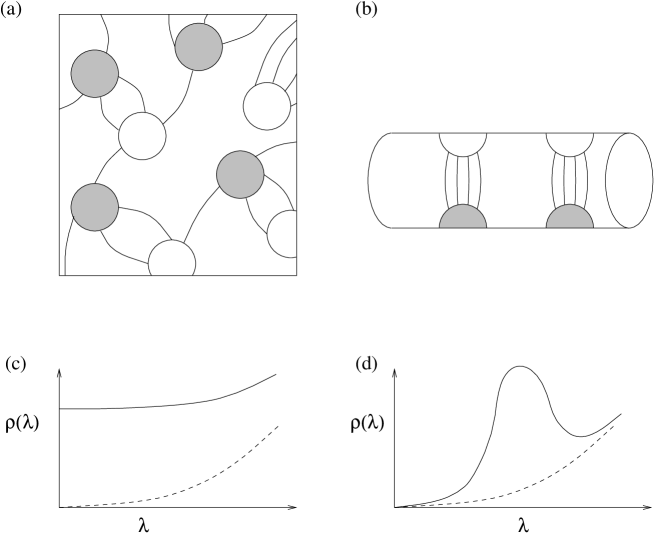
FIG. 1.: Schematic picture of the instanton liquid at zero temperature (a) and above the chiral phase transition (b). Instantons and anti-instantons are shown as open and shaded circles. The lines correspond to fermion exchanges. Figures (c) and (d) show the schematic form of the Dirac spectrum in the configurations (a) and (b).

The significance of the quark condensate is the fact that it is an order parameter for the spontaneous breakdown of chiral symmetry in the QCD vacuum. The gluon condensate is important because the QCD trace anomaly

$$T_{\mu\mu} = \sum_{f}m_{f}\langle\bar{q}_{f}q_{f}\rangle-\frac{b}{32\pi^{2}}\langle g^{2}G^{2}\rangle$$ (3)

relates this quantity to the energy density $\epsilon_{0}\simeq-500\,{\rm MeV}/{\rm fm}^{3}$ of the QCD vacuum. Here, $T_{\mu\nu}$ is the energy momentum tensor and $b=11N_{c}/3-2N_{f}/3$ is the first coefficient of the beta function.

Any model of the QCD vacuum should explain the origin and value of these condensates, the mechanism for confinement and chiral symmetry breaking and its relation to the underlying parameters of the theory (the scale parameter and the matter content of the theory). Most of the early attempts to understand the QCD ground state were based on the idea that the vacuum is dominated by classical gauge field configurations, for example constant fields [Sav_77] or regions of constants fields patched together, as in the Spaghetti vacuum introduced by the Kopenhagen group [AO_80]. All of these attempts were unsuccessful, however, because constant fields were found to be unstable against quantum perturbations.

Instantons are classical solutions to the euclidean equations of motion. They are characterized by a topological quantum number and correspond to tunneling events between degenerate classical vacua in Minkowski space. As in quantum mechanics, tunneling lowers the ground state energy. Therefore, instantons provide a simple understanding of the negative non-perturbative vacuum energy density. In the presence of light fermions, instantons are associated with fermionic zero modes. Zero modes not only play a crucial role in understanding the axial anomaly, they are also intimately connected with spontaneous chiral symmetry breaking. When instantons interact through fermion exchanges, zero modes can become delocalized, forming a collective quark condensate.

A crude picture of quark motion in the vacuum can then be formulated as follows (see Fig. 1a). Instantons act as a potential well, in which light quarks can form bound states (the zero modes). If instantons form an interacting liquid, quarks can travel over large distances by hopping from one instanton to another, similar to electrons in a conductor. Just like the conductivity is determined by the density of states near the Fermi surface, the quark condensate is given by the density of eigenstates of the Dirac operator near zero virtuality. A schematic plot of the distribution of eigenvalues of the Dirac operator is shown in Fig. 1c. For comparison, the spectrum of the Dirac operator for non-interacting quarks is depicted by the dashed line. If the distribution of instantons in the QCD vacuum is sufficiently random, there is a non-zero density of eigenvalues near zero and chiral symmetry is broken.

The quantum numbers of the zero modes produce very specific correlations between quarks. First, since there is exactly one zero mode per flavor, quarks with different flavor (say $u$ and $d$) can travel together, but quarks with the same flavor cannot. Furthermore, since zero modes have a definite chirality (left handed for instantons, right handed for anti-instantons), quarks flip their chirality as they pass through an instanton. This is very important phenomenologically, because it distinguishes instanton effects from perturbative interactions, in which the chirality of a massless quark does not change. It also implies that quarks can only be exchanged between instantons of the opposite charge.

Based on this picture, we can also understand the formation of hadronic bound states. Bound states correspond to poles in hadronic correlation functions. As an example, let us consider the pion, which has the quantum numbers of the current $j_{\pi}=\bar{u}\gamma_{5}d$. The correlation function $\Pi(x)=\langle j_{\pi}(x)j_{\pi}(0)\rangle$ is the amplitude for an up quark and a down anti-quark with opposite chiralities created by a source at point 0 to meet again at the point $x$. In a disordered instanton liquid, this amplitude is large, because the two quarks can propagate by the process shown in Fig. 2a. As a result, there is a light pion state. For the $\rho$ meson, on the other hand, we need the amplitude for the propagation of two quarks with the same chirality. This means that the quarks have to be absorbed by different instantons (or propagate in non-zero mode states), see Fig. 2c. The amplitude is smaller, and the meson state is much less tightly bound.

FIG. 2.: Instanton contribution to hadronic correlation functions Fig. a) shows the pion, b) the nucleon and c) the rho meson correlator. The solid lines correspond to zero mode contributions to the quark propagator.

Using this picture, we can also understand the formation of a bound nucleon. Part of the proton wave function is a scalar $ud$ diquark coupled to another $u$ quark. This means that the nucleon can propagate as shown in Fig. 2b. The vertex in the scalar diquark channel is identical to the one in the pion channel with one of the quark lines reversed The $\Delta$ resonance has the quantum numbers of a vector diquark coupled to a third quark. Just like in the case of the $\rho$ meson, there is no first order instanton induced interaction, and we expect the $\Delta$ to be less bound than than the nucleon.

The paradigm discussed here bears striking similarity to one of the oldest approaches to hadronic structure, the Nambu-Jona-Lasinio (NJL) model [NJL_61]. In analogy with the Bardeen-Cooper-Schrieffer theory of superconductivity, it postulates a short-range attractive force between fermions (nucleons in the original model and light quarks in modern versions). If this interaction is sufficiently strong, it can rearrange the vacuum and the ground state becomes superconducting, with a non-zero quark condensate. In the process, nearly massless current quarks become effectively massive constituent quarks. The short range interaction can then bind these constituent quarks into hadrons (without confinement).

This brief outline indicates that instantons provide at least a qualitative understanding of many features of the QCD ground state and its hadronic excitations. How can this picture be checked and made more quantitive? Clearly, two things need to be done. First, a consistent instanton ensemble has to be constructed in order to make quantitative predictions for hadronic observables. Second, we would like to test the underlying assumption that the topological susceptibility, the gluon condensate, chiral symmetry breaking etc. are dominated by instantons. This can be done most directly on the lattice. We will discuss both of these issues in the main part of this review, sections III-VI.

4 QCD at finite temperature

Properties of the QCD vacuum, like the vacuum energy density, the quark and gluon condensate are not directly accessible to experiment. Measuring non-perturbative properties of the vacuum requires the possibility to compare the system with the ordinary, perturbative state. This state of matter has not existed in nature since the Big Bang, so experimental attempts at studying the perturbative phase of QCD have focused on recreating miniature Big Bangs in relativistic heavy ion collisions.

The basic idea is that at sufficiently high temperature or density, QCD will undergo a phase transition to a new state, referred to as the quark gluon plasma, in which chiral symmetry is restored and quarks and gluon are deconfined. The temperature scale for this transition is set by the vacuum energy density and pressure of the vacuum. For the perturbative vacuum to have a pressure comparable to the vacuum pressure $500\,{\rm MeV}/{\rm fm}^{3}$, a temperature on the order of $150-200\,{\rm MeV}$ is required. According to our current understanding, such temperatures are reached in the ongoing or planned experiments at the AGS (about 2+2 GeV per nucleon in the center of mass system), CERN SPS (about 10+10 GeV) or RHIC (100+100 GeV).

In order to interpret these experiments, we need to understand the properties of hadrons and hadronic matter near and above the phase transition. As for cold matter, this requires an understanding of the ground state and how the rearrangement of the vacuum that causes chiral symmetry to be restored takes place. A possible mechanism for chiral symmetry restoration in the instanton liquid is indicated in Fig. 1b,d. At high temperature, instantons and anti-instantons have a tendency to bind in pairs that are aligned along the (euclidean) time direction. The corresponding quark eigenstates are strongly localized and chiral symmetry is unbroken. There is some theoretical evidence for this picture which will be discussed in detail in section VII. In particular, there is evidence from lattice simulations that instantons do not disappear at the phase transition, but only at even higher temperatures. This implies that instantons affect properties of the quark gluon plasma at temperatures not too far above the phase transition.

C The history of instantons

In books and reviews, physical theories are usually presented as a systematic development, omitting the often confusing history of the subject. The history of instantons also did not follow a straight path. Early enthusiasm concerning the possibility to understand non-perturbative phenomena in QCD, in particular confinement, caused false hopes, which led to years of frustration. Only many years later did work on phenomenological aspects of instantons lead to breakthroughs. In the following we will try to give a brief tour of the two decades that have passed since the discovery of instantons.

1 Discovery and early applications

The instanton solution of the Yang-Mills equations was discovered by Polyakov and coworkers [BPS_75], motivated by the search for classical solutions with nontrivial topology in analogy with the ’t Hooft-Polyakov monopole [Pol_75]. Shortly thereafter, a number of authors clarified the physical meaning of the instanton as a tunneling event between degenerate classical vacua [JR_76, CDG_76, Pol_77]. These works also introduced the concept of $\theta$-vacua in connection with QCD.

Some of the early enthusiasm was fueled by Polyakov’s discovery that instantons cause confinement in certain 3-dimensional models [Pol_77]. However, it was soon realized that this is not the case in 4-dimensional gauge theories. An important development originated with ’t Hooft’s classic paper [tHo_76], in which he calculated the semi-classical tunneling rate. In this context, he discovered the presence of zero modes in the spectrum of the Dirac operator. This result implied that tunneling is intimately connected with light fermions, in particular that every instanton absorbs one left handed fermion of every species, and emits a right handed one (and vice versa for anti-instantons). This result also explained how anomalies, for example the violation of axial charge in QCD and baryon number in electroweak theory, are related to instantons.

In his work, ’t Hooft estimated the tunneling rate in electroweak theory, where the large Higgs expectation value guarantees the validity of the semi-classical approximation, and found it to be negligible. Early attempts to study instantons effects in QCD, where the rate is much larger but also harder to estimate, were summarized in [CDG_78]. These authors realized that the instanton ensemble can be described as a 4-dimensional “gas” of pseudo-particles that interact via forces that are dominantly of dipole type. While they were not fully successful in constructing a consistent instanton ensemble, they nevertheless studied a number of important instanton effects: the instanton induced potential between heavy quarks, the possibility that instantons cause the spontaneous breakdown of chiral symmetry, and instanton corrections to the running coupling constant.

One particular instanton-induced effect, the anomalous breaking of $U(1)_{A}$ symmetry and the $\eta^{\prime}$ mass, deserves special attention. Witten and Veneziano wrote down an approximate relation that connects the $\eta^{\prime}$ mass with the topological susceptibility [Wit_79, Ven_79]. This was a very important step, because it was the first quantitative result concerning the effect of the anomaly on the $\eta^{\prime}$ mass. However, it also caused some confusion, because the result had been derived using the large $N_{c}$ approximation, which is not easily applied to instantons. In fact, both Witten and Veneziano expressed strong doubts concerning the relation between the topological susceptibility and instantons, suggesting that instantons are not important dynamically [Wit_79b].

2 Phenomenology leads to a qualitative picture

By the end of the 70’s the general outlook was very pessimistic. There was no experimental evidence for instanton effects, and no theoretical control over semi-classical methods in QCD. If a problem cannot be solved by direct theoretical analysis, it often useful to turn to a more phenomenological approach. By the early 80’s, such an approach to the structure of the QCD vacuum became available with the QCD sum rule method [SVZ_79]. QCD sum rules relate vacuum parameters, in particular the quark and gluon condensates, to the behavior of hadronic correlation functions at short distances. Based on this analysis, it was realized that “all hadrons are not alike” [NSVZ_81]. The Operator Product Expansion (OPE) does not give reliable predictions for scalar and pseudo-scalar channels ($\pi,\sigma,\eta,\eta^{\prime}$ as well as scalar and pseudo-scalar glueballs). These are precisely the channels that receive direct instanton contributions [GI_80, NSVZ_81, Shu_83].

In order to understand the available phenomenology, a qualitative picture, later termed the instanton liquid model, was proposed in [Shu_82]. In this work, the two basic parameters of the instanton ensemble were suggested: the mean density of instantons is $n\simeq 1\,{\rm fm}^{-4}$, while their average size is $\rho\simeq 1/3$ fm. This means that the space time volume occupied by instantons $f\sim n\rho^{4}$ is small; the instanton ensemble is dilute. This observation provides a small expansion parameter which we can use in order to perform systematic calculations.

Using the instanton liquid parameters $n\simeq 1\,{\rm fm}^{-4},\,\rho\simeq 1/3$ fm we can reproduce the phenomenological values of the quark and gluon condensates. In addition to that, one can calculate direct instanton corrections to hadronic correlation functions at short distance. The results were found to be in good agreement with experiment in both attractive ($\pi,K$) and repulsive ($\eta^{\prime}$) pseudo-scalar meson channels [Shu_83].

3 Technical development during the 80’s

Despite its phenomenological success, there was no theoretical justification for the instanton liquid model. The first steps towards providing some theoretical basis for the instanton model were taken in [IMP_81, DP_84]. These authors used variational techniques and the mean field approximation (MFA) to deal with the statistical mechanics of the instanton liquid. The ensemble was stabilized using a phenomenological core [IMP_81] or a repulsive interaction derived from a specific ansatz for the gauge field interaction [DP_84]. The resulting ensembles were found to be consistent with the phenomenological estimates.

The instanton ensemble in the presence of light quarks was studied in [DP_86]. This work introduced the picture of the quark condensate as a collective state built from delocalized zero modes. The quark condensate was calculated using the mean field approximation and found to be in agreement with experiment. Hadronic states were studied in the random phase approximation (RPA). At least in the case of pseudo-scalar mesons, the results were also in good agreement with experiment.

In parallel, numerical methods for studying the instanton liquid were developed [Shu_88]. Numerical simulations allow one to go beyond the MF and RPA approximations and include the ’t Hooft interaction to all orders. This means that one can also study hadronic channels that, like vector mesons, do not have first order instanton induced interactions, or channels, like the nucleon, that are difficult to treat in the random phase approximation.

Nevertheless, many important aspects of the model remain to be understood. This applies in particular to the theoretical foundation of the instanton liquid model. When the instanton-anti-instanton interaction was studied in more detail, it became clear that there is no classical repulsion in the gauge field interaction. A well separated instanton-anti-instanton pair is connected to the perturbative vacuum by a smooth path [BY_86, Ver_91]. This means that the instanton ensemble cannot be stabilized by purely classical interactions. This is related to the fact that in general, it is not possible to separate non-perturbative (instanton-induced) and perturbative effects. Only in special cases, like in quantum mechanics (Sec. II A 5) and supersymmetric field theory (Sec. VIII C) has this separation been accomplished.

4 Recent progress

In the past few years, a great deal was learned about instantons in QCD. The instanton liquid model with the parameters mentioned above, now referred to as the random instanton liquid model (RILM), was used for large-scale, quantitative calculations of hadronic correlation functions in essentially all meson and baryon channels [SV_93b, SSV_94]. Hadronic masses and coupling constants for most of the low-lying mesons and baryon states were shown to be in quantitative agreement with experiment.

The next surprise came from a comparison of the correlators calculated in the random model and first results from lattice calculations [CGHN_93a]. The results agree quantitatively not only in channels that were already known from phenomenology, but also in others (such as the nucleon and delta), were no previous information (except for the particle masses, of course) existed.

These calculations were followed up by direct studies of the instanton liquid on the lattice. Using a procedure called cooling, one can extract the classical content of strongly fluctuating lattice configurations. Using cooled configurations, the MIT group determined the main parameters of the instanton liquid [CGHN_94]. Inside the accuracy involved ($\sim 10\%$) the density and average size coincide with the values suggested a decade earlier. In the mean time, these numbers have been confirmed by other calculations (see Sec. III C). In addition to that, it was shown that the agreement between lattice correlation functions and the instanton model was not a coincidence: the correlators are essentially unaffected by cooling. This implies that neither perturbative (removed by cooling) nor confinement (strongly reduced) forces are crucial for hadronic properties.

Technical advances in numerical simulation of the instanton liquid led to the construction of a self-consistent, interacting instanton ensemble, which satisfies all the general constraints imposed by the trace anomaly and chiral low energy theorems [SV_95, SS_96, SS_96b]. The corresponding unquenched (with fermion vacuum bubbles included) correlation functions significantly improve the description of the $\eta^{\prime}$ and $\delta$ mesons, which are the two channels where the random model fails completely.

Finally, significant progress was made in understanding the instanton liquid at finite temperature and the mechanism for the chiral phase transition. It was realized earlier that at high temperature, instantons should be suppressed by Debye screening [Shu_78, PY_80]. Therefore, it was generally assumed that chiral symmetry restoration is a consequence of the disappearance of instantons at high temperature.

More recently it was argued that up to the critical temperature, the density of instantons should not be suppressed [SV_94]. This prediction was confirmed by direct lattice measurements of the topological susceptibility [CS_95], which indeed found little change in the topological susceptibility for $T<T_{c}$, and the expected suppression for $T>T_{c}$. If instantons are not suppressed around $T_{c}$, a different mechanism for the chiral phase transition is needed. It was suggested that chiral symmetry is restored because the instanton liquid is rearranged, going from a random phase below $T_{c}$ to a correlated phase of instanton-anti-instanton molecules above $T_{c}$ [IS_94, SSV_95]. This idea was confirmed in direct simulations of the instanton ensemble, and a number of consequences of the scenario were explored.

D Topics that are not discussed in detail

There is a vast literature on instantons (the SLAC database lists over 3000 references, which probably does not include the more mathematically oriented works) and limitations of space and time as well as our expertise have forced us to exclude many interesting subjects from this review. Our emphasis in writing this review has been on the theory and phenomenology of instantons in QCD. We discuss instantons in other models only to the extent that they are pedagogically valuable or provide important lessons for QCD. Let us mention a few important omissions and give a brief guide to the relevant literature:

1. Direct manifestations of small-size instantons in high energy baryon number violating (BNV) reactions. The hope is that in these processes, one may observe rather spectacular instanton effects in a regime where reliable semi-classical calculations are possible. In the electroweak theory, instantons lead to baryon number violation, but the amplitude for this reaction is strongly suppressed at low energies. It was hoped that this suppression can be overcome at energies on the order of the sphaleron barrier $E\simeq 10$ TeV, but the emerging consensus is that this dramatic phenomenon will not be observable. Some of the literature is mentioned in Sec. VIII B, see also the recent review [Aoy_97].

2. A related problem is the transition from tunneling to thermal activation and the calculation of the Sphaleron rate at high temperature. This question is of interest in connection with baryogenesis in the early universe and axial charge fluctuations in the quark gluon plasma. A recent discussion can be found in the review [Smi_96].

3. The decay of unstable vacua in quantum mechanics or field theory [Col_77]. A more recent review can be found in [Aoy_97].

4. Direct instanton contributions to deep inelastic scattering and other hard processes in QCD, see [BB_93, BB_95] and the review [RS_94].

5. Instanton inspired models of hadrons, or phenomenological lagrangians supplemented by the ’t Hooft interaction. These models include NJL models [HK_94], soliton models [DPP_88, CBK_96], potential models [BBH_90], bag models [DZK_92], etc.

6. Mathematical aspects of instantons [EGH_80], the ADHM construction of the most general $n$-instanton solution [AHDM_77], constrained instantons [Aff_81], instantons and four-manifolds [FU_84], the connection between instantons and solitons [AM_89]. For a review of known solutions of the classical Yang-Mills field equations in both Euclidean and Minkowski space we refer the reader to [Act_79].

7. Formal aspects of the supersymmetric instanton calculus, spinor techniques, etc. This material is covered in [NSV_83, NSV_83b, Nov_87, AKM_88].

8. The strong CP problem, bounds on the theta parameter, the axion mechanism [PQ_77], etc. Some remarks on these questions can be found in Sec. II C 3.

II Semi-classical theory of tunneling

A Tunneling in quantum mechanics

1 Quantum mechanics in Euclidean space

This section serves as a brief introduction into path integral methods and can easily be skipped by readers familiar with the subject. We will demonstrate the use of Feynman diagrams in a simple quantum mechanical problem, which does not suffer from any of the divergencies that occur in field theory. Indeed, we hope that this simple example will find its way into introductory field theory courses.

Another point we would like to emphasize in this section is the similarity between quantum and statistical mechanics. Qualitatively, both quantum and statistical mechanics deal with variables that are subject to random fluctuations (quantum or thermal), so that only ensemble averaged quantities make sense. Formally the connection is related to the similarity between the statistical partition function ${\rm tr}[\exp(-\beta H)]$ and the generating functional (6) (see below) describing the dynamical evolution of a quantum system.

Consider the simplest possible quantum mechanical system, the motion of a particle of mass $m$ in a time independent potential $V(x)$. The standard approach is based on an expansion in terms of stationary states $\psi_{n}(x)$, given as solutions of the Schrödinger equation $H\psi_{n}=E_{n}\psi_{n}$. Instead, we will concentrate on another object, the Green’s function

$$G(x,y,t) = \langle y|\exp(-iHt)|x\rangle,$$ (4)

which is the amplitude for a particle to go from point $x$ at time $t=0$ to point $y$ at time $t$. The Green’s function can be expanded in terms of stationary states

$$G(x,y,t) = \sum_{n=1}^{\infty}\psi_{n}^{*}(x)\psi_{n}(y)\exp(-iE_{n}t).$$ (5)

This representation has many nice features that are described in standard text books on quantum mechanics. There is, however, another representation which is more useful in order to introduce semi-classical methods and to deal with system with many degrees of freedom, the Feynman path integral [FH_65]

$$G(x,y,t) = \int Dx(t)\,\exp(iS[x(t)]).$$ (6)

Here, the Green’s functions is given as a sum over all possible paths $x(t)$ leading from $x$ at $t=0$ to $y$ at time $t$. The weight for the paths is provided by the action $S=\int dt[m\dot{x}^{2}/2-V(x)]$. One way to provide a more precise definition of the path integral is to discretize the path. Dividing the time axis into $N$ intervals, $a=t/N$, the path integral becomes an $N$-dimensional integral over $x_{n}=x(t_{n}=an)\;n=1,\ldots,N$. The discretized action is given by

$$S = \sum_{n}\left[\frac{m}{2a}(x_{n}-x_{n-1})^{2}-aV(x_{n})\right].$$ (7)

This form is not unique, other discretizations with the same continuum limit can also be used. The path integral is now reduced to a multiple integral over $x_{n}$, where we have to take the limit $n\to\infty$. In general, only Gaussian integrals can be done exactly. In the case of the harmonic oscillator $V(x)=m\omega^{2}x^{2}/2$ one finds [FH_65]

$$G_{osc}(x,y,t) = \left(\frac{m\omega}{2\pi i\sin\omega t}\right)^{1/2}\exp\left[\left(\frac{im\omega}{2\sin\omega t}\right)\left((x^{2}+y^{2})\cos(\omega t)-2xy\right)\right]$$ (8)

In principal, the discretized action (7) should be amenable to numerical simulations. In practice, the strongly fluctuating phase in (6) renders this approach completely useless. There is, however, a simple way to get around the problem. If one performs an analytic continuation of $G(x,y,t)$ to imaginary (Euclidean) time $\tau=it$, the weight function becomes $\exp(-S_{E}[x(\tau)])$ with the Euclidean action $S_{E}=\int dt[m(dx/d\tau)^{2}/2+V(x)]$. In this case, we have a positive definite weight and numerical simulations, even for multidimensional problems, are feasible. Note that the relative sign of the kinetic and potential energy terms in the Euclidean action has changed, making it look like a Hamiltonian. In Euclidean space, the discretized action (7) looks like the energy functional of a 1-dimensional spin chain with nearest neighbor interactions. This observation provides the formal link between an $n$-dimensional statistical system and Euclidean quantum (field) theory in $(n-1)$ dimensions.

Euclidean Green’s functions can be interpreted in terms of “thermal” distributions. If we use periodic boundary conditions ($x=y$) and integrate over $x$ we obtain the statistical sum

$$\int dx\,G(x,x,\tau) = \sum_{n=1}^{\infty}\exp(-E_{n}\tau),$$ (9)

where the time interval $\tau$ plays the role of an inverse temperature $\tau=T^{-1}$. In particular, $G(x,x,1/T)$ has the physical meaning of a probability distribution for $x$ at temperature $T$. For the harmonic oscillator mentioned above, the Euclidean Green’s function is

$$G_{osc}(x,y,\tau) = \left(\frac{m\omega}{2\pi\sinh\omega\tau}\right)^{1/2}\exp\left[-\left(\frac{m\omega}{2\sinh\omega\tau}\right)\left((x^{2}+y^{2})\cosh(\omega\tau)-2xy\right)\right]$$ (10)

For $x=y$, the spatial distribution is Gaussian at any $T$, with a width $\langle x^{2}\rangle=\frac{1}{2m\omega}\coth(\omega/2T)$. If $\tau$ is very large, the effective temperature is small and the ground state dominates. From the exponential decay, we can read off the ground state energy $E_{0}=\omega/2$ and from the spatial distribution the width of the ground state wave function $\langle x^{2}\rangle=(2m\omega)^{-1}$. At high $T$ we get the classical result $\langle x^{2}\rangle=T/(m\omega^{2})$.

FIG. 3.: Feynman diagrams for the energy (a) and the Green’s function (b) of the anharmonic oscillator.

Non-Gaussian path integrals cannot be done exactly. As long as the non-linearities are small, we can use perturbation theory. Consider an anharmonic oscillator with (Euclidean) action

$$S_{E} = \int d\tau\,\left[{\dot{x}^{2}\over 2}+{\omega^{2}x^{2}\over 2}+\alpha x^{3}+\beta x^{4}\right]$$ (11)

Expanding the path integral in powers of $\alpha$ and $\beta$ one can derive the Feynman rules for the anharmonic oscillator. The free propagator is given by

$$G_{0}(\tau_{1},\tau_{2}) = \langle x(\tau_{1})x(\tau_{2})\rangle\;=\;{1\over 2\omega}\exp(-\omega|\tau_{1}-\tau_{2}|).$$ (12)

In addition to that, there are three and four-point vertices with coupling constants $\alpha$ and $\beta$. To calculate an $n$-point Green’s function we have to sum over all diagrams with $n$ external legs and integrate over the time variables corresponding to internal vertices.

The vacuum energy is given by the sum of all closed diagrams. At one loop order, there is only one diagram, the free particle loop diagram. At two loop order, there are two $O(\alpha^{2})$ and one $O(\beta)$ diagram, see Fig. 3a. The calculation of the diagrams is remarkably simple. Since the propagator is exponentially suppressed for large times, everything is finite. Summing all the diagrams, we get

$$\langle 0|\exp(-H\tau)|0\rangle\;=\;\sqrt{\frac{\omega}{\pi}}\exp\left(-\frac{\omega\tau}{2}\right)\left[1-\left(\frac{3\beta}{4\omega^{2}}-\frac{11\alpha^{2}}{8\omega^{4}}\right)\tau+\ldots\right]$$ (13)

For small $\alpha^{2},\beta$ and $\tau$ not too large, we can exponentiate the result and read off the correction to the ground state energy

$$E_{0} = \frac{\omega}{2}+\frac{3\beta}{4\omega^{2}}-\frac{11\alpha^{2}}{8\omega^{4}}+\ldots.$$ (14)

Of course, we could have obtained the result using ordinary Rayleigh-Schrödinger perturbation theory, but the method discussed here proves to be much more powerful when we come to non-perturbative effects and field theory.

One more simple exercise is worth mentioning: the evaluation of first perturbative correction to the Green’s function. The diagrams shown in Fig. 3b give

$$\Delta G_{0}(0,\tau) = {9\alpha^{2}\over 4\omega^{6}}+{\alpha^{2}\over 2\omega^{6}}e^{-2\omega\tau}+{15\alpha^{2}\over 4\omega^{5}}\tau e^{-\omega\tau}-{3\beta\over 2\omega^{3}}\tau e^{-\omega\tau}$$ (15)

Comparing the result with the decomposition in terms of stationary states

$$G(0,\tau) = \sum_{n=0}^{\infty}e^{-(E_{n}-E_{0})\tau}|\langle 0|x|n\rangle|^{2}$$ (16)

we can identify the first (time independent) term with the square of the ground state expectation value $\langle 0|x|0\rangle$ (which is non-zero due to the tadpole diagram). The second term comes from the excitation of 2 quanta, and the last two (with extra factors of $\tau$) are the lowest order “mass renormalization”, or corrections to the zero order gap between the ground and first excited states, $E_{1}-E_{0}=\omega$.

2 Tunneling in the double well potential

Tunneling phenomena in quantum mechanics were discovered by George Gamow in the late 20’s in the context of alpha-decay. He introduced the exponential suppression factor that explained why a decay governed by the Coulomb interaction (with a typical nuclear time scale of $10^{-22}$ sec) could lead to lifetimes of millions of years. Tunneling is a quantum mechanical phenomenon, a particle penetrating a classically forbidden region. Nevertheless, we will describe the tunneling process using classical equations of motion. Again, the essential idea is to continue the transition amplitude to imaginary time.

Let us give a qualitative argument why tunneling can be treated as a classical process in imaginary time. The energy of a particle moving in the potential $V(x)$ is given by $E=p^{2}/(2m)+V(x)$, and in classical mechanics only regions of phase space where the kinetic energy is positive are accessible. In order to reach the classically forbidden region $E<V$, the kinetic energy would have to be negative, corresponding to imaginary momentum $p$. In the semi-classical (WKB) approximation to quantum mechanics, the wave function is given by $\psi(x)\sim\exp[i\Phi(x)]$ with $\Phi(x)=\pm\int^{x}dx^{\prime}\,p(x^{\prime})+O(\hbar)$ where $p(x)=(2m)^{1/2}(E-V(x))^{1/2}$ is the local classical momentum. In the classically allowed region, the wave function is oscillatory, while in the classically forbidden region (corresponding to imaginary momenta) it is exponentially suppressed.

There is another way to introduce imaginary momenta, which is more easily generalized to multidimensional problems and field theory, by considering motion in imaginary time. Continuing $\tau=it$, the classical equation of motion is given by

$$m\frac{d^{2}x}{d\tau^{2}} = +\frac{dV}{dx},$$ (17)

where the sign of the potential energy term has changed. This means that classically forbidden regions are now classically allowed. The distinguished role of the classical tunneling path becomes clear if one considers the Feynman path integral. Although any path is allowed in quantum mechanics, the path integral is dominated by paths that maximize the weight factor $\exp(-S[x_{cl}(\tau)])$, or minimize the Euclidean action. The classical path is the path with the smallest possible action.

Let us consider a widely used toy model, the double-well potential

$$V = \lambda(x^{2}-\eta^{2})^{2}$$ (18)

with minima at $\pm\eta$, the two ”classical vacua” of the system. Quantizing around the two minima, we would find two degenerate states localized at $x=\pm\eta$. Of course, we know that this is not the correct result. Tunneling will mix the two states, the true ground state is (approximately) the symmetric combination, while the first excited state is the antisymmetric combination of the two states.

It is easy to solve the equations of motion in imaginary time and obtain the classical tunneling solution

$$x_{cl}(\tau) = \eta\tanh\left[\frac{\omega}{2}(\tau-\tau_{0})\right],$$ (19)

which goes from $x(-\infty)=-\eta$ to $x(\infty)=\eta$. Here, $\tau_{0}$ is a free parameter (the instanton center) and $\omega^{2}=8\lambda\eta^{2}$. The action of the solution is $S_{0}=\omega^{3}/(12\lambda)$. We will refer to the path (19) as the instanton, since (unlike a soliton) the solution is localized in time. An anti-instanton solution is given by $x^{A}_{cl}(\tau)=-x^{I}_{cl}(\tau)$. It is convenient to re-scale the time variable such that $\omega=1$ and shift $x$ such that one of the minima is at $x=0$. In this case, there is only one dimensionless parameter, $\lambda$, and since $S_{0}=1/(12\lambda)$, the validity of the semi-classical expansion is controlled by $\lambda\ll 1$.

The semi-classical approximation to the path integral is obtained by systematically expanding around the classical solution

$$\langle-\eta|e^{-H\tau}|\eta\rangle = e^{-S_{0}}\int Dx(\tau)\,\exp\left(-\frac{1}{2}\delta x\left.\frac{\delta^{2}S}{\delta x^{2}}\right|_{x_{cl}}\!\!\!\delta x+\ldots\right).$$ (20)

Note that the linear term is absent, because $x_{cl}$ is a solution of the equations of motion. Also note that we implicitly assume $\tau$ to be large, but smaller than the typical lifetime for tunneling. If $\tau$ is larger than the lifetime, we have to take into account multi-instanton configurations, see below. Clearly, the tunneling amplitude is proportional to $\exp(-S_{0})$. The pre-exponent requires the calculation of fluctuations around the classical instanton solution. We will study this problem in the following section.

3 Tunneling amplitude at one loop order

In order to take into account fluctuations around the classical path, we have to calculate the path integral

$$\int[D\delta x]\exp\left(-\frac{1}{2}\int d\tau\;\delta x(\tau)O\delta x(\tau)\right)$$ (21)

where $O$ is the differential operator

$$O = -\frac{1}{2}\frac{d^{2}}{d\tau^{2}}+\left.\frac{d^{2}V}{dx^{2}}\right|_{x=x_{cl}}.$$ (22)

This calculation is somewhat technical, but it provides a very good illustration of the steps that are required to solve the more difficult field theory problem. We follow here the original work [Pol_77] and the review [VZN_82]. A simpler method to calculate the determinant is described in the appendix of Coleman’s lecture notes [Col_77].

The integral (21) is Gaussian, so it can be done exactly. Expanding the differential operator $O$ in some basis $\{x_{i}(\tau)\}$, we have

$$\int\left(\prod_{n}dx_{n}\right)\,\exp\left(-\frac{1}{2}\sum_{ij}x_{i}O_{ij}x_{j}\right) = (2\pi)^{n/2}\left(\det O\right)^{-1/2}$$ (23)

The determinant can be calculated by diagonalizing $O$, $Ox_{n}(\tau)=\epsilon_{n}x_{n}(\tau)$. This eigenvalue equation is just a one-dimensional Schrödinger equation

$$\left(-{d^{2}\over d\tau^{2}}+\omega^{2}\left[1-\frac{3}{2\cosh^{2}(\omega\tau/2)}\right]\right)x_{n}(\tau) = \epsilon_{n}x_{n}(\tau)$$ (24)

There are two bound states plus a continuum of scattering states. The lowest eigenvalue is $\epsilon_{0}=0$, and the other bound state is at $\epsilon_{1}={3\over 4}\omega^{2}$. The eigenfunction of the zero energy state is

$$x_{0}(\tau) = \sqrt{\frac{3\omega}{8}}\frac{1}{\cosh^{2}(\omega\tau/2)},$$ (25)

where we have normalized the wave function, $\int d\tau x_{n}^{2}=1$. There should be a simple explanation for the presence of a zero mode. Indeed, the appearance of a zero mode is related to translational invariance, the fact that the action does not depend on the location $\tau_{0}$ of the instanton. The zero mode wave function is just the derivative of the instanton solution over $\tau_{0}$

$$x_{0}(\tau)=-S_{0}^{-1/2}\frac{d}{d\tau_{0}}x_{cl}(\tau-\tau_{0}),$$ (26)

where the normalization follows from the fact that the classical solution has zero energy. If one of the eigenvalues is zero this means that the determinant vanishes and the tunneling amplitude is infinite! However, the presence of a zero mode also implies that there is one direction in functional space in which fluctuations are large, so the integral is not Gaussian. This means that the integral in that direction should not be performed in Gaussian approximation, but has to be done exactly.

This can be achieved by replacing the integral over the expansion parameter $c_{0}$ associated with the zero mode direction (we have parameterized the path by $x(\tau)=\sum_{n}c_{n}x_{n}(\tau)$) with an integral over the collective coordinate $\tau_{0}$. Using

$$dx = \frac{dx_{cl}}{d\tau_{0}}d\tau_{0}\;=\;-\sqrt{S_{0}}x_{0}(\tau)d\tau_{0}$$ (27)

and $dx=x_{0}dc_{0}$ we have $dc_{0}=\sqrt{S_{0}}d\tau_{0}$. The functional integral over the quantum fluctuation is now given by

$$\int[D\delta x(\tau)]\,\exp(-S) = \left[\prod_{n>0}\left(\frac{2\pi}{\epsilon_{n}}\right)\right]^{1/2}\sqrt{S_{0}}\int d\tau_{0},$$ (28)

where the first factor, the determinant with the zero mode excluded, is often referred to as $\det^{\prime}O$. The result shows that the tunneling amplitude grows linearly with time. This is as it should be, there is a finite transition probability per unit time.

The next step is the calculation of the non-zero mode determinant. For this purpose we make the spectrum discrete by considering a finite time interval $[-\tau_{m}/2,\tau_{m}/2]$ and imposing boundary conditions at $\pm\tau_{m}/2$: $x_{n}(\pm\tau_{m}/2)=0$. The product of all eigenvalues is divergent, but the divergence is related to large eigenvalues, independent of the detailed shape of the potential. The determinant can be renormalized by taking the ratio over the determinant of the free harmonic oscillator. The result is

$$\left(\frac{\det\left[-\frac{d^{2}}{d\tau^{2}}+V^{\prime\prime}(x_{cl})\right]}{\det\left[-\frac{d^{2}}{d\tau^{2}}+\omega^{2}\right]}\right)^{-1/2} = \sqrt{\frac{S_{0}}{2\pi}}\;\omega\int d\tau_{0}\;\left(\frac{\det^{\prime}\left[-\frac{d^{2}}{d\tau^{2}}+V^{\prime\prime}(x_{cl})\right]}{\omega^{-2}\det\left[-\frac{d^{2}}{d\tau^{2}}+\omega^{2}\right]}\right)^{-1/2}$$ (29)

where we have eliminated the zero mode from the determinant and replaced it by the integration over $\tau_{0}$. We also have to extract the lowest mode from the harmonic oscillator determinant, which is given by $\omega^{2}$. The next eigenvalue is $3\omega^{2}/4$, while the corresponding oscillator mode is $\omega^{2}$ (up to corrections of order $1/\tau_{m}^{2}$, that are not important as $\tau_{m}\to\infty$). The rest of the spectrum is continuous as $\tau_{m}\to\infty$. The contribution from these states can be calculated as follows.

The potential $V^{\prime\prime}(x_{cl})$ is localized, so for $\tau\to\pm\infty$ the eigenfunctions are just plane waves. This means we can take one of the two linearly independent solutions to be $x_{p}(\tau)\sim\exp(ip\tau)$ as $\tau\to\infty$. The effect of the potential is to give a phase shift

$$x_{p}(\tau) = \exp(ip\tau+i\delta_{p})\hskip 14.22636pt\tau\to-\infty,$$ (30)

where, for this particular potential, there is no reflected wave. The phase shift is given by [LL]

$$\exp(i\delta_{p}) = {1+ip/\omega\over 1-ip/\omega}{1+2ip/\omega\over 1-2ip/\omega}.$$ (31)

The second independent solution is obtained by $\tau\rightarrow-\tau$. The spectrum is determined by the quantization condition $x(\pm\tau_{m}/2)=0$, which gives

$$p_{n}\tau_{m}-\delta_{p_{n}}=\pi n,$$ (32)

while the harmonic oscillator modes are determined by $p_{n}\tau_{m}=\pi n$. If we denote the solutions of (32) by $\tilde{p}_{n}$, the ratio of the determinants is given by

$$\prod_{n}\left[{\omega^{2}+\tilde{p}_{n}^{2}\over\omega^{2}+p_{n}^{2}}\right] = \exp\left(\sum_{n}\log\left[\frac{\omega^{2}+\tilde{p}_{n}^{2}}{\omega^{2}+p_{n}^{2}}\right]\right)\;=\;\exp\left({1\over\pi}\int_{0}^{\infty}{2pdp\,\delta_{p}\over p^{2}+\omega^{2}}\right)\;=\;\frac{1}{9}.$$ (33)

where we have expanded the integrand in the small difference $\tilde{p}_{n}-p_{n}=\delta_{p_{n}}/\tau_{m}$ and changed from summation over $n$ to an integral over $p$. In order to perform the integral, it is convenient to integrate by part and use the result for $(d\delta_{p})/(dp)$. Collecting everything, we finally get

$$\langle-\eta|e^{-H\tau_{m}}|\eta\rangle = \left[\sqrt{\frac{\omega}{\pi}}\exp\left(-\frac{\omega\tau_{m}}{2}\right)\right]\left[\sqrt{\frac{6S_{0}}{\pi}}\exp\left(-S_{0}\right)\right]\left(\omega\tau_{m}\right),$$ (34)

where the first factor comes from the harmonic oscillator amplitude and the second is the ratio of the two determinants.

The result shows that the transition amplitude is proportional to the time interval $\tau_{m}$. In terms of stationary states, this is due to the fact that the contributions from the two lowest states almost cancel each other. The ground state wave function is the symmetric combination $\Psi_{0}(x)=(\phi_{-\eta}(x)+\phi_{\eta}(x))/\sqrt{2}$, while the first excited state $E_{1}=E_{0}+\Delta E$ is antisymmetric, $\Psi_{1}(x)=(\phi_{-\eta}(x)-\phi_{\eta}(x))/\sqrt{2}$. Here, $\phi_{\pm\eta}$ are the harmonic oscillator wave functions around the two classical minima. For times $\tau\ll 1/\Delta E$, the tunneling amplitude is given by

$$\langle-\eta|e^{-H\tau_{m}}|\eta\rangle = \Psi_{0}^{*}(-\eta)\Psi_{0}(\eta)e^{-E_{0}\tau_{m}}+\Psi_{1}^{*}(-\eta)\Psi_{1}(\eta)e^{-E_{1}\tau_{m}}+\ldots$$ (35)

$$= \frac{1}{2}\phi^{*}_{-\eta}(-\eta)\phi_{\eta}(\eta)(\Delta E\tau_{m})e^{-\omega\tau_{m}/2}+\ldots.$$ (36)

Note that the validity of the semi-classical approximation requires $\tau\gg 1/\omega$.

We can read off the level-splitting from (34) and (36). The result can be obtained in an even more elegant way by going to large times $\tau>1/\Delta E$. In this case, multi-instanton paths are important. If we ignore the interaction between instantons, multi instanton contributions can easily be summed up

$$\langle-\eta|e^{-H\tau_{m}}|\eta\rangle = \sqrt{\frac{\omega}{\pi}}e^{-\omega\tau_{m}/2}\sum_{n\,{\rm odd}}\int\limits_{-\tau_{m}/2<\tau_{1}<\ldots<\tau_{m}/2}\left[\prod_{i=1}^{n}\omega d\tau_{i}\right]\left(\sqrt{\frac{6S_{0}}{\pi}}\exp(-S_{0})\right)^{n}$$ (37)

$$= \sqrt{\frac{\omega}{\pi}}e^{-\omega\tau_{m}/2}\sum_{n\,{\rm odd}}\frac{(\omega\tau_{m}d)^{n}}{n!}\;=\;\sqrt{\frac{\omega}{\pi}}e^{-\frac{\omega\tau_{m}}{2}}\sinh\left(\omega\tau_{m}d\right),$$ (38)

where $d=(6S_{0}/\pi)^{1/2}\exp(-S_{0})$. Summing over all instantons simply leads to the exponentiation of the tunneling rate. Now we can directly read off the level splitting

$$\Delta E = \sqrt{\frac{6S_{0}}{\pi}}\omega\exp\left(-S_{0}\right).$$ (39)

If the tunneling rate increases, $1/\Delta E\simeq 1/\omega$, interactions between instantons become important. We will study this problem in Sec. II A 5.

4 The tunneling amplitude at two-loop order

The WKB method can be used to systematically calculate higher orders in $1/S_{0}$. Beyond leading order, however, the WKB method becomes quite tedious, even when applied to quantum mechanics. In this subsection we show how the $1/S_{0}$ correction to the level splitting in the double well can be determined using a two loop instanton calculation. We follow here [WS_94], which corrected a few mistakes in the earlier literature [AS_87, Ole_89]. Numerical simulations were performed in [Shu_88c] while the correct result was first obtained using different methods by [ZJ_81].

FIG. 4.: Feynman diagrams for the two-loop correction to the tunneling amplitude in the quantum mechanical double well potential. The first three correspond to the diagrams in Fig. 3a, but with different propagators and vertices, while the forth diagram contains a new vertex, generated by the collective coordinate Jacobian.

To next order in $1/S_{0}$, the tunneling amplitude can be decomposed as

$$\langle-\eta|e^{-H\tau}|\eta\rangle \simeq \left|\psi_{0}(\eta)\right|^{2}\left(1+\frac{2A}{S_{0}}+\ldots\right)\exp\left(-\frac{\omega\tau}{2}\left[1+\frac{B}{S_{0}}+\ldots\right]\right)\Delta E_{0}\left(1+\frac{C}{S_{0}}+\ldots\right)\tau,$$ (40)

where we are interested in the coefficient $C$, the next order correction to the level splitting. The other two corrections, $A$ and $B$ are unrelated to tunneling and we can get rid of them by dividing the amplitude by $\langle\eta|\exp(-H\tau)|\eta\rangle$, see (15).

In order to calculate the next order correction to the instanton result, we have to expand the action beyond order $(\delta x)^{2}$. The result can be interpreted in terms of a new set of Feynman rules in the presence of an instanton (see Fig. 4). The triple and quartic coupling constants are $\alpha=4\lambda x_{cl}(t)$ and $\beta=\lambda$ (compared to $\alpha_{0}=4\lambda\eta=\sqrt{2\lambda}$ and $\beta_{0}=\lambda$ for the anharmonic oscillator). The propagator is the Green’s function of the differential operator (22). There is one complication due to the fact that the operator $O$ has a zero mode. The Green’s function is uniquely defined by requiring it to be orthogonal to the translational zero mode. The result is [Ole_89]

$$(2\omega)G(x,y) = g_{0}(x,y)\left[2-xy+\frac{1}{4}|x-y|(11-3xy)+(x-y)^{2}\right]+\frac{3}{8}\left(1-x^{2}\right)\left(1-y^{2}\right)\left[\log\left(g_{0}(x,y)\right)-\frac{11}{3}\right]$$ (42)

$$\hskip 28.45274ptg_{0}(x,y)\;=\;\frac{1-|x-y|-xy}{1+|x-y|-xy}$$

where $x=\tanh(\omega t/2),\,y=\tanh(\omega t^{\prime}/2)$ and $g_{0}(x,y)$ is the Green’s function of the harmonic oscillator (12). There are four diagrams at two-loop order, see Fig. 4. The first three diagrams are of the same form as the anharmonic oscillator diagrams. Subtracting these contributions, we get

$$a_{1} = -3\beta_{0}\int^{\infty}_{-\infty}dt\,\left(G^{2}(t,t)-G^{2}_{0}(t,t)\right)\;=\;-\frac{97}{1680}S_{0}^{-1}$$ (43)

$$b_{11} = 3\alpha_{0}^{2}\int^{\infty}_{-\infty}\int^{\infty}_{-\infty}dtdt^{\prime}\,\left(\tanh(t/2)\tanh(t^{\prime}/2)G^{3}(t,t^{\prime})-G^{3}_{0}(t,t^{\prime})\right)\;=\;-\frac{53}{1260}S_{0}^{-1}$$ (44)

$$b_{12} = \frac{9}{2}\alpha_{0}^{2}\int^{\infty}_{-\infty}\int^{\infty}_{-\infty}dtdt^{\prime}\,\left(\alpha^{2}\tanh(t/2)\tanh(t^{\prime}/2)G(t,t)G(t,t^{\prime})G(t^{\prime},t^{\prime})-G_{0}(t,t)G_{0}(t,t^{\prime})G_{0}(t^{\prime},t^{\prime})\right)\;=\;-\frac{39}{560}S_{0}^{-1}.$$ (45)

The last diagram comes from expanding the Jacobian in $\delta x$. This leads to a tadpole graph proportional to $\ddot{x}_{cl}$, which has no counterpart in the anharmonic oscillator case. We get

$$c_{1} = -9\beta_{0}\int^{\infty}_{-\infty}\int^{\infty}_{-\infty}dtdt^{\prime}\,\frac{\tanh(t/2)}{\cosh^{2}(t/2)}\tanh(t^{\prime}/2)G(t,t^{\prime})G(t^{\prime},t^{\prime})\;=\;-\frac{49}{60}S_{0}^{-1}.$$ (46)

The sum of the four diagrams is $C=(a_{1}+b_{11}+b_{12}+c_{1})S_{0}=-71/72$. The two-loop result for the level splitting is

$$\Delta E = \sqrt{\frac{6S_{0}}{\pi}}\omega\exp\left(-S_{0}-\frac{71}{72}\frac{1}{S_{0}}+\ldots\right),$$ (47)

in agreement with the WKB result obtained in [ZJ_81]. The fact that the next order correction is of order one and negative is significant. It implies that the one-loop result becomes inaccurate for moderately large barriers ($S\sim 1$), and that it overestimates the tunneling probability. We have presented this calculation in detail in order to show that the instanton method can be systematically extended to higher orders in $1/S$. In field theory, however, this calculation is sufficiently difficult that it has not yet been performed.

5 Instanton-anti-instanton interaction and the ground state energy

Up to now we focused on the tunneling amplitude for transitions between the two degenerate vacua of the double well potential. This amplitude is directly related to the gap $\Delta E$ between the ground state and the first excited state. In this subsection we wish to discuss how the semi-classical theory can be used to calculate the mean $E_{ctr}=(E_{0}+E_{1})/2$ of the two levels. In this context, it is customary to define the double well potential by $V=(x^{2}/2)(1-gx)^{2}$. The coupling constant $g$ is related to the coupling $\lambda$ used above by $g^{2}=2\lambda$. Unlike the splitting, the mean energy is related to topologically trivial paths, connecting the same vacua. The simplest non-perturbative path of this type is an instanton-anti-instanton pair.

In section II A 3 we calculated the tunneling amplitude using the assumption that instantons do not interact with each other. We found that tunneling makes the coordinates uncorrelated, and leads to a level splitting. If we take the interaction among instantons into account, the contribution from instanton-anti-instanton pairs is given by

$$\langle\eta|e^{-H\tau_{m}}|\eta\rangle = \tau_{m}\int\frac{d\tau}{\pi g^{2}}\,\exp\left(S_{IA}(\tau)\right),$$ (48)

where $S_{IA}(\tau)$ is the action of an instanton-anti-instanton pair with separation $\tau$ and the prefactor $(\pi g^{2})^{-1}$ comes from the square of the single instanton density. The action of an instanton anti-instanton (IA) pair can be calculated given an ansatz for the path that goes from one minimum of the potential to the other and back. An example for such a path is the “sum ansatz” [ZJ_83]

$$x_{sum}(\tau) = \frac{1}{2g}\left(2-\tanh\left(\frac{\tau-\tau_{I}}{2}\right)+\tanh\left(\frac{\tau-\tau_{A}}{2}\right)\right).$$ (49)

This path has the action $S_{IA}(T)=1/g^{2}(1/3-2e^{-T}+O(e^{-2T}))$, where $T=|\tau_{I}-\tau_{A}|$. It is qualitatively clear that if the two instantons are separated by a large time interval $T\gg 1$, the action $S_{IA}(T)$ is close to $2S_{0}$. In the opposite limit $T\rightarrow 0$, the instanton and the anti-instanton annihilate and the action $S_{IA}(T)$ should tend to zero. In that limit, however, the IA pair is at best an approximate solution of the classical equations of motion and it is not clear how the path should be chosen.

FIG. 5.: Streamline configurations in the double well potential for $\eta=1.4$ and $\lambda=1$ ($\omega\simeq 4$, $S_{0}\simeq 5$), adapted from [Shu_88c]. The horizontal axis shows the time coordinate and the vertical axis the amplitude $x(\tau)$. The different paths correspond to different values of the streamline parameter $\lambda$ as the configuration evolves from a well separated pair to an almost perturbative path. The initial path has an action $S=1.99S_{0}$, the other paths correspond to a fixed reductions of the action by $0.2S_{0}$.

FIG. 6.: Distribution of the action density $s=\dot{x}^{2}/2+V(x)$ for the streamline configurations shown in Fig. 5.

The best way to deal with this problem is the “streamline” or “valley” method [BY_86]. In this approach one starts with a well separated IA pair and lets the system evolve using the method of steepest descent. This means that we have to solve

$$f(\lambda)\frac{dx_{\lambda}(\tau)}{d\lambda} = \frac{\delta S}{\delta x_{\lambda}(\tau)},$$ (50)

where $\lambda$ labels the path as we proceed from the initial configuration $x_{\lambda=0}(\tau)=x_{sum}(\tau)$ down the valley to the vacuum configuration and $f(\lambda)$ is an arbitrary function that reflects the reparametrization invariance of the streamline solution. A sequence of paths obtained by solving the streamline equation (50) numerically is shown in Fig. 5 [Shu_88c]. An analytical solution to first order in $1/S_{0}$ can be found in [BY_86]. The action density $s=\dot{x}^{2}/2+V(x)$ corresponding to the paths in Fig. 5 is shown in Fig. 6. We can see clearly how the two localized solutions merge and eventually disappear as the configuration progresses down the valley. Using the streamline solution, the instanton-anti-instanton action for large $T$ is given by [FS_95]

$$S(T) = \frac{1}{g^{2}}\Big{[}\frac{1}{3}-2e^{-T}-12Te^{-2T}+O(e^{-2T})\Big{]}+\Big{[}24Te^{-T}+O(e^{-T})\Big{]}+\Big{[}\frac{71g^{2}}{6}+O(g^{4})\Big{]},$$ (51)

where the first term is the classical streamline interaction up to next-to-leading order, the second term is the quantum correction (one loop) to the leading order interaction, and the last term is the two-loop correction to the single instanton interaction.

If one tries to use the instanton result (48) in order to calculate corrections to $E_{ctr}$ one encounters two problems. First, the integral diverges at large $T$. This is simply related to the fact that IA pairs with large separation should not be counted as pairs, but as independent instantons. This problem is easily solved, all one has to do is subtract the square of the single instanton contribution. Second, once this subtraction has been performed, the integral is dominated by the region of small $T$, where the action is not reliably calculable. This problem is indeed a serious one, related to the fact that $E_{ctr}$ is not directly related to tunneling, but is dominated by perturbative contributions. In general, we expect $E_{ctr}$ to have an expansion

$$E_{ctr} = \sum_{k}g^{2k}E^{(0)}_{ctr,\,k}+e^{-2/(6g^{2})}\sum_{k}g^{2k}E^{(2)}_{ctr,\,k}+\ldots,$$ (52)

where the first term is the perturbative contribution, the second corresponds to one IA pair, and so on. However, perturbation theory in $g$ is divergent (not even Borel summable), so the calculation of the IA contribution requires a suitable definition of perturbation theory.

One way to deal with this problem (going back to Dyson’s classical work on QED) is analytic continuation in $g$. For $g$ imaginary ($g^{2}$ negative), the $IA$ contribution is well defined (the integral over $T$ is dominated by $T\sim-\log(-g^{2})$). The IA contribution to $E_{ctr}$ is [Bog_80, ZJ_83]

$$E^{(2)}_{ctr} = \frac{e^{-1/(3g^{2})}}{\pi g^{2}}\left[\log\left(-\frac{2}{g^{2}}\right)+\gamma+O(g^{2}\log(g^{2}))\right],$$ (53)

where $\gamma=0.577\ldots$ is Euler’s constant. When we now continue back to positive $g^{2}$, we get both real and imaginary contributions to $E_{ctr}$. Since the sum of all contributions to $E_{ctr}$ is certainly real, the imaginary part has to cancel against a small $O(e^{-1/(3g^{2})})$ imaginary part in the perturbative expansion. This allows us to determine the imaginary part ${\rm Im}E_{ctr}^{(0)}$ of the analytically continued perturbative sum.

From the knowledge of the imaginary part of perturbation theory, one can determine the large order behavior of the perturbation series $E^{(0)}_{ctr}=\sum_{k}g^{2k}E^{(0)}_{ctr,\,k}$ [Lip_77, BPZ_77]. The coefficients are given by the dispersion integrals

$$E^{(0)}_{ctr,\,k} = \frac{1}{\pi}\int_{0}^{\infty}{\rm Im}\left(E^{(0)}_{ctr,\,k}(g^{2})\right)\frac{dg^{2}}{g^{2k+2}}.$$ (54)

Since the semi-classical result (53) is reliable for small $g$, we can calculate the large order coefficients. Including the corrections calculated in [FS_95], we have

$$E^{(0)}_{ctr,\,k} = {3^{k+1}k\!\over\pi}\left(1-\frac{53}{18k}+\ldots\right).$$ (55)

The result can be compared with the exact coefficients [BPZ_77]. For small $k$ the result is completely wrong, but already for $k=5,6,7,8$ the ratio of the asymptotic result to the exact coefficients is $1.04,\,1.11,\,1.12,\,1.11$. We conclude that instantons determine the large order behavior of the perturbative expansion. This is in fact a generic result: the asymptotic behavior of perturbation theory is governed by semi-classical configurations (although not necessarily involving instantons).

TABLE I.: Exact center of the band energies $E_{ctr}=(E_{0}+E_{1})/2$ for different values of $g^{2}$ (expressed in terms of $N=1/(3g^{2})$) compared to the semiclassical estimate discussed in the text.

$N\equiv 1/(3g^{2})$	4	6	8	10	12
$E_{ctr}^{ex}$	0.4439	0.43797	0.44832	0.459178	0.467156
$E_{ctr}^{th}$	0.4367	0.44367	0.44933	0.459307	0.467173

In order to check the instanton-anti-instanton result (53) against the numerical value of $E_{ctr}$ for different values of $g$ we have to subtract the perturbative contribution to $E_{ctr}$. This can be done using analytic continuation and the Borel transform [ZJ_82], and the result is in very good agreement with the instanton calculation. A simpler way to check the instanton result was proposed by [FS_95]. These authors simply truncate the perturbative series at the $N$-th term. In this case, the best accuracy occurs when $|N-1/3g^{2}|\sim 1$ and the estimate for $E_{ctr}$ is given by

$$E_{ctr} = \sum_{n=0}^{N}g^{2n}E_{ctr,\,n}^{(0)}+\frac{3Ne^{-N}}{\pi}\left[\log(6N)+\gamma+\frac{1}{3}\sqrt{\frac{2\pi}{N}}\right]\left(1-\frac{53}{18N}\right),$$ (56)

which is compared to the exact values in the table I. We observe that the result (56) is indeed very accurate, and that the error is on the order of $e^{-N}=e^{-1/3g^{2}}$.

In summary: $E_{ctr}$ is related to configurations with no net topology, and in this case the calculation of instanton effects requires a suitable definition of the perturbation series. This can be accomplished using analytic continuation in the coupling constant. After analytic continuation, we can perform a reliable interacting instanton calculation, but the the result has an imaginary part. This shows that the instanton contribution by itself is not well determined, it depends on the definition of the perturbation sum. However, the sum of perturbative and non-perturbative contributions is well defined (and real) and agrees very accurately with the numerical value of $E_{ctr}$.

In gauge theories the situation is indeed very similar: there are both perturbative and non-perturbative contributions to the vacuum energy and the two contributions are not clearly separated. However, in the case of gauge theories, we do not know how to define perturbation theory, so we are not yet able to perform a reliable calculation of the vacuum energy, similar to eq.(56).

B Fermions coupled to the double well potential

In this section we will consider one fermionic degree of freedom $\psi_{\alpha}$ ($\alpha=1,2$) coupled to the double well potential. This model provides additional insight into the vacuum structure not only of quantum mechanics, but also of gauge theories: we will see that fermions are intimately related to tunneling, and that the fermion-induced interaction between instantons leads to strong instantons-anti-instantons correlations. Another motivation for studying fermions coupled to the double well potential is that for a particular choice of the coupling constant, the theory is supersymmetric. This means that perturbative corrections to the vacuum energy cancel, and the instanton contribution is more easily defined.

The model is defined by the action

$$S = \frac{1}{2}\int dt\,\left(\dot{x}^{2}+{W^{\prime}}^{2}+\psi\dot{\psi}+cW^{\prime\prime}\psi\sigma_{2}\psi\right),$$ (57)

where $\psi_{\alpha}\,(\alpha=1,2)$ is a two component spinor, dots denote time and primes spatial derivatives, and $W^{\prime}=x(1-gx)$. We will see that the vacuum structure depends crucially on the Yukawa coupling $c$. For $c=0$ fermions decouple and we recover the double well potential studied in the previous sections, while for $c=1$ the classical action is supersymmetric. The supersymmetry transformation is given by

$$\delta x=\zeta\sigma_{2}\psi,\hskip 28.45274pt\delta\psi=\sigma_{2}\zeta\dot{x}-W^{\prime}\zeta,$$ (58)

where $\zeta$ is a Grassmann variable. For this reason, $W$ is usually referred to as the superpotential. The action (57) can be rewritten in terms of two bosonic partner potentials [SH_81, CKS_95]. Nevertheless, it is instructive to keep the fermionic degree freedom, because the model has many interesting properties that also apply to QCD, where the action cannot be bosonized.

As before, the potential $V=\frac{1}{2}{W^{\prime}}^{2}$ has degenerate minima connected by the instanton solution. The tunneling amplitude is given by

$${\rm Tr}\left(e^{-\beta H}\right) = \int d\tau\,J\,\frac{\sqrt{\det{\cal O}_{F}}}{\sqrt{\det{\cal O}^{\prime}_{B}}}\,e^{-S_{cl}},$$ (59)

where $S_{cl}$ is the classical action, ${\cal O}_{B}$ is the bosonic operator (22) and ${\cal O}_{F}$ is the Dirac operator

$${\cal O}_{F} = \frac{d}{dt}+c\sigma_{2}W^{\prime\prime}(x_{cl}).$$ (60)

As explained in Sec. II A 3, ${\cal O}_{B}$ has a zero mode, related to translational invariance. This mode has to be treated separately, which leads to a Jacobian $J$ and an integral over the corresponding collective coordinate $\tau$. The fermion determinant also has a zero mode, given by

$$\chi^{I,A} = N\exp\left(\mp\int_{-\infty}^{t}dt^{\prime}\,cW^{\prime\prime}(x_{cl})\right)\frac{1}{\sqrt{2}}\left(\begin{array}[]{c}1\\ \mp i\end{array}\right).$$ (63)

Since the fermion determinant appears in the numerator of the tunneling probability, the presence of a zero mode implies that the tunneling rate is zero!

The reason for this is simple: the two vacua have different fermion number, so they cannot be connected by a bosonic operator. The tunneling amplitude is non-zero only if a fermion is created during the process, $\langle 0,+|\psi_{+}|0,-\rangle$, where $\psi_{\pm}=\frac{1}{\sqrt{2}}(\psi_{1}\pm i\psi_{2})$ and $|0,\pm\rangle$ denote the corresponding eigenstates. Formally, we get a finite result because the fermion creation operator absorbs the zero mode in the fermion determinant. As we will see later, this mechanism is completely analogous to the axial $U(1)_{A}$ anomaly in QCD and baryon number violation in electroweak theory. For $c=1$, the tunneling rate is given by [SH_81]

$$\langle 0,+|\psi_{+}|0,-\rangle = \frac{1}{\sqrt{\pi g^{2}}}e^{-\frac{1}{6g^{2}}}$$ (64)

This result can be checked by performing a direct calculation using the Schrödinger equation.

Let us now return to the calculation of the ground state energy. For $c=0$, the vacuum energy is the sum of perturbative contributions and a negative non-perturbative shift $O(e^{-1/(6g^{2})})$ due to individual instantons. For $c\neq 0$, the tunneling amplitude (64) will only enter squared, so one needs to consider instanton-anti-instanton pairs. Between the two tunneling events, the system has an excited fermionic state, which causes a new interaction between the instantons. For $c=1$, supersymmetry implies that all perturbative contributions (including the zero-point oscillation) to the vacuum energy cancel. Using supersymmetry, one can calculate the vacuum energy from the tunneling rate (64) [SH_81]. The result is $O(e^{-1/(3g^{2})})$ and positive, which implies that supersymmetry is broken. While the dependence on $g$ is what we would expect for a gas of instanton-anti-instanton molecules, understanding the sign in the context of an instanton calculation is more subtle (see below).

It is an instructive exercise to calculate the vacuum energy numerically (which is quite straightforward, we are still dealing with a simple quantum mechanical toy model). In general, the vacuum energy is non-zero, but for $c\to 1$, the vacuum energy is zero up to exponentially small corrections. Varying the coupling constant, one can verify that the vacuum energy is smaller than any power in $g^{2}$, showing that supersymmetry breaking is a non-perturbative effect.

For $c\neq 1$ the instanton-anti-instanton contribution to the vacuum energy has to be calculated directly. Also, even for $c=1$, where the result can be determined indirectly, this is a very instructive calculation. For an instanton-anti-instanton path, there is no fermionic zero mode. Writing the fermion determinant in the basis spanned by the original zero modes of the individual pseudo-particles, we have

$${\det}\left({\cal O}_{F}\right)_{ZMZ} = \left(\begin{array}[]{cc}0&T_{IA}\\ T_{AI}&0\end{array}\right),$$ (67)

where $T_{IA}$ is the overlap matrix element

$$T_{IA} = \int_{-\infty}^{\infty}dt\,\chi_{A}\left(\partial_{t}+c\sigma_{2}W^{\prime\prime}(x_{IA}(t))\right)\chi_{I}.$$ (68)

Clearly, mixing between the two zero modes shifts the eigenvalues away from zero and the determinant is non-zero. As before, we have to choose the correct instanton-anti-instanton path $x_{IA}(t)$ in order to evaluate $T_{IA}$. Using the valley method introduced in the last section the ground state energy is given by [BY_86]

$$E = \frac{1}{2}\left(1-c+O(g^{2})\right)-\frac{1}{2\pi}e^{-\frac{1}{3g^{2}}}\left(\frac{g^{2}}{2}\right)^{c-1}2c^{c}\int_{0}^{\infty}d\tau\,\exp\left(-2c(\tau-\tau_{0})+\frac{2}{g^{2}}e^{-2\tau}\right),$$ (69)

where $\tau$ is the instanton-anti-instanton separation and $\exp(-2\tau_{0})=cg^{2}/2$. The two terms in the exponent inside the integral corresponds to the fermionic and bosonic interaction between instantons. One can see that fermions cut off the integral at large $\tau$. There is an attractive interaction which grows with distance and forces instantons and anti-instantons to be correlated. Therefore, for $c\neq 0$ the vacuum is no longer an ensemble of random tunneling events, but consists of correlated instanton-anti-instanton molecules.

The fact that both the bosonic and fermionic interaction is attractive means that the integral (69), just like (48), is dominated by small $\tau$ where the integrand is not reliable. This problem can be solved as outlined in the last section, by analytic continuation in the coupling constant. As an alternative, Balitsky and Yung suggested to shift the integration contour in the complex $\tau$-plane, $\tau\rightarrow\tau+i\pi/2$. On this path, the sign of the bosonic interaction is reversed and the fermionic interaction picks up a phase factor $\exp(ic\pi)$. This means that there is a stable saddle point, but the instanton contribution to the ground state energy is in general complex. The imaginary part cancels against the imaginary part of the perturbation series, and only the sum of the two contributions is well defined.

A special case is the supersymmetric point $c=1$. In this case, perturbation theory vanishes and the contribution from instanton-anti-instanton molecules is real,

$$E=\frac{1}{2\pi}e^{-\frac{1}{3g^{2}}}\left(1+O(g^{2})\right).$$ (70)

This implies that at the SUSY point $c=1$, there is a well defined instanton-anti-instanton contribution. The result agrees with what one finds from the $H=\frac{1}{2}\{Q_{+},Q_{-}\}$ relation or directly from the Schrödinger equation.

In summary: In the presence of light fermions, tunneling is possible only if the fermion number changes during the transition. Fermions create a long-range attractive interaction between instantons and anti-instantons and the vacuum is dominated by instanton-anti-instanton “molecules”. It is non-trivial to calculate the contribution of these configurations to the ground state energy, because topologically trivial paths can mix with perturbative corrections. The contribution of molecules is most easily defined if one allows the collective coordinate (time separation) to be complex. In this case, there exists a saddle point where the repulsive bosonic interaction balances the attractive fermionic interaction and molecules are stable. These objects give a non-perturbative contribution to the ground state energy, which is in general complex, except in the supersymmetric case where it is real and positive.

C Tunneling in Yang-Mills theory

1 Topology and classical vacua

Before we study tunneling phenomena in Yang-Mills theory, we have to become more familiar with the classical vacuum of the theory. In the Hamiltonian formulation, it is convenient to use the temporal gauge $A_{0}=0$ (here we use matrix notation $A_{i}=A_{i}^{a}\lambda^{a}/2$, where the $SU(N)$ generators satisfy $[\lambda^{a},\lambda^{b}]=2if^{abc}\lambda^{c}$ and are normalized according to ${\rm Tr}(\lambda^{a}\lambda^{b})=2\delta^{ab}$). In this case, the conjugate momentum to the field variables $A_{i}(x)$ is just the electric field $E_{i}=\partial_{0}A_{i}$. The Hamiltonian is given by

$$H = \frac{1}{2g^{2}}\int d^{3}x\,(E_{i}^{2}+B_{i}^{2}),$$ (71)

where $E_{i}^{2}$ is the kinetic and $B_{i}^{2}$ the potential energy term. The classical vacuum corresponds to configurations with zero field strength. For non-abelian gauge fields this does not imply that the potential has to be constant, but limits the gauge fields to be “pure gauge”

$$A_{i} = iU(\vec{x})\partial_{i}U(\vec{x})^{\dagger}.$$ (72)

In order to enumerate the classical vacua we have to classify all possible gauge transformations $U(\vec{x})$. This means that we have to study equivalence classes of maps from 3-space $R^{3}$ into the gauge group $SU(N)$. In practice, we can restrict ourselves to matrices satisfying $U(\vec{x})\to 1$ as $x\to\infty$ [CDG_78]. Such mappings can be classified using an integer called the winding (or Pontryagin) number, which counts how many times the group manifold is covered

$$n_{W} = \frac{1}{24\pi^{2}}\int d^{3}x\,\epsilon^{ijk}{\rm Tr}\left[(U^{\dagger}\partial_{i}U)(U^{\dagger}\partial_{j}U)(U^{\dagger}\partial_{k}U)\right].$$ (73)

In terms of the corresponding gauge fields, this number is the Chern-Simons characteristic

$$n_{CS} = \frac{1}{16\pi^{2}}\int d^{3}x\,\epsilon^{ijk}\left(A_{i}^{a}\partial_{j}A_{k}^{a}+\frac{1}{3}f^{abc}A_{i}^{a}A_{j}^{b}A_{k}^{c}\right).$$ (74)

Because of its topological meaning, continuous deformations of the gauge fields do not change $n_{CS}$. In the case of $SU(2)$, an example of a mapping with winding number $n$ can be found from the “hedgehog” ansatz

$$U(\vec{x}) = \exp(if(r)\tau^{a}\hat{x}^{a}).$$ (75)

where $r=|\vec{x}|$ and $\hat{x}^{a}=x^{a}/r$. For this mapping, we find

$$n_{W} = \frac{2}{\pi}\int dr\,\sin^{2}(f)\frac{df}{dr}\,=\,\frac{1}{\pi}\left[f(r)-\frac{\sin(2f(r))}{2}\right]_{0}^{\infty}.$$ (76)

In order for $U(\vec{x})$ to be uniquely defined, $f(r)$ has to be a multiple of $\pi$ at both zero and infinity, so that $n_{W}$ is indeed an integer. Any smooth function with $f(r\to\infty)=0$ and $f(0)=n\pi$ provides an example for a function with winding number $n$.

We conclude that there is an infinite set of classical vacua enumerated by an integer $n$. Since they are topologically different, one cannot go from one vacuum to another by means of a continuous gauge transformation. Therefore, there is no path from one vacuum to another, such that the energy remains zero all the way.

2 Tunneling and the BPST instanton

Two important questions concerning the classical vacua immediately come to mind. First, is there some physical observable which distinguishes between them? Second, is there any way to go from one vacuum to another? The answer to the first one is positive, but most easily demonstrated in the presence of light fermions, so we will come to it later. Let us now concentrate on the second one.

We are going to look for a tunneling path in gauge theory, which connects topologically different classical vacua. From the quantum mechanical example we know that we have to look for classical solutions of the euclidean equations of motion. The best tunneling path is the solution with minimal euclidean action connecting vacua with different Chern-Simons number. To find these solutions, it is convenient to exploit the following identity

$$S = \frac{1}{4g^{2}}\int d^{4}x\,G^{a}_{\mu\nu}G^{a}_{\mu\nu}\;=\;\frac{1}{4g^{2}}\int d^{4}x\,\left[\pm G^{a}_{\mu\nu}\tilde{G}^{a}_{\mu\nu}+\frac{1}{2}\left(G^{a}_{\mu\nu}\mp\tilde{G}^{a}_{\mu\nu}\right)^{2}\right],$$ (77)

where $\tilde{G}_{\mu\nu}=1/2\epsilon_{\mu\nu\rho\sigma}G_{\rho\sigma}$ is the dual field strength tensor (the field tensor in which the roles of electric and magnetic fields are interchanged). Since the first term is a topological invariant (see below) and the last term is always positive, it is clear that the action is minimal if the field is (anti) self-dual

$$G^{a}_{\mu\nu} = \pm\tilde{G}^{a}_{\mu\nu},$$ (78)

One can also show directly that the self-duality condition implies the equations of motion, $D_{\mu}G_{\mu\nu}=0$. This is a useful observation, because in contrast to the equation of motion, the self-duality equation (78) is a first order differential equation. In addition to that, one can show that the energy momentum tensor vanishes for self-dual fields. In particular, self-dual fields have zero (Minkowski) energy density.

The action of a self-dual field configuration is determined by the topological charge (or 4 dimensional Pontryagin index)

$$Q = {1\over 32\pi^{2}}\int d^{4}x\,G^{a}_{\mu\nu}\tilde{G}^{a}_{\mu\nu}$$ (79)

From (77), we have $S=(8\pi^{2}|Q|)/g^{2}$ for self-dual fields. For finite action field configurations, $Q$ has to be an integer. This can be seen from the fact that the integrand is a total derivative

$$Q = {1\over 32\pi^{2}}\int d^{4}x\,G^{a}_{\mu\nu}\tilde{G}^{a}_{\mu\nu}\;=\;\int d^{4}x\,\partial_{\mu}K_{\mu}\;=\;\int d\sigma_{\mu}K_{\mu},$$ (81)

$$\hskip 28.45274ptK_{\mu}\;=\;{1\over 16\pi^{2}}\epsilon_{\mu\alpha\beta\gamma}\left(A^{a}_{\alpha}\partial_{\beta}A^{a}_{\gamma}+{1\over 3}f^{abc}A^{a}_{\alpha}A^{b}_{\beta}A^{c}_{\gamma}\right).$$

For finite action configurations, the gauge potential has to be pure gauge at infinity $A_{\mu}\to iU\partial_{\mu}U^{\dagger}$. Similar to the arguments given in the last section, all maps from the three sphere $S_{3}$ (corresponding to $|x|\to\infty$) into the gauge group can be classified by a winding number $n$. Inserting $A_{\mu}=iU\partial_{\mu}U^{\dagger}$ into (81) one finds that $Q=n$.

Furthermore, if the gauge potential falls off sufficiently rapid at spatial infinity,

$$Q = \int dt{d\over dt}\int d^{3}xK_{0}\;=\;n_{CS}(t=\infty)-n_{CS}(t=-\infty)$$ (82)

which shows that field configurations with $Q\neq 0$ connect different topological vacua. In order to find an explicit solution with $Q=1$, it is useful to start from the simplest winding number $n=1$ configuration. Similar to (75), we can take $A_{\mu}=iU\partial_{\mu}U^{\dagger}$ with $U=i\hat{x}_{\mu}\tau_{\mu}^{+}$, where $\tau_{\mu}^{\pm}=(\vec{\tau},\mp i)$. Then $A_{\mu}^{a}=2\eta_{a\mu\nu}x_{\nu}/x^{2}$, where we have introduced the ’t Hooft symbol $\eta_{a\mu\nu}$. It is defined by

$$\eta_{a\mu\nu} = \left\{\begin{array}[]{rcl}\epsilon_{a\mu\nu}&&\mu,\,\nu=1,\,2,\,3,\\ \delta_{a\mu}&&\nu=4,\\ -\delta_{a\nu}&&\mu=4.\end{array}\right.$$ (86)

We also define $\overline{\eta}_{a\mu\nu}$ by changing the sign of the last two equations. Further properties of $\eta_{a\mu\nu}$ are summarized in appendix A 3. We can now look for a solution of the self-duality equation (78) using the ansatz $A_{\mu}^{a}=2\eta_{a\mu\nu}x_{\nu}f(x^{2})/x^{2}$, where $f$ has to satisfy the boundary condition $f\to 1$ as $x^{2}\to\infty$. Inserting the ansatz in (78), we get

$$f(1-f)-x^{2}f^{\prime} = 0.$$ (87)

This equation is solved by $f=x^{2}/(x^{2}+\rho^{2})$, which gives the BPST instanton solution [BPS_75]

$$A^{a}_{\mu}(x)=\frac{2\eta_{a\mu\nu}x_{\nu}}{x^{2}+\rho^{2}}.$$ (88)

Here $\rho$ is an arbitrary parameter characterizing the size of the instanton. A solution with topological charge $Q=-1$ can be obtained by replacing $\eta_{a\mu\nu}\to\overline{\eta}_{a\mu\nu}$. The corresponding field strength is

$$(G^{a}_{\mu\nu})^{2} = \frac{192\rho^{4}}{(x^{2}+\rho^{2})^{4}}.$$ (89)

In our conventions, the coupling constant only appears as a factor in front of the action. This convention is very convenient in dealing with classical solutions. For perturbative calculations, it is more common to rescale the fields as $A_{\mu}\to gA_{\mu}$. In this case, there is a factor $1/g$ in the instanton gauge potential, which shows that the field of the instanton is much stronger than ordinary, perturbative, fields.

Also note that $G^{a}_{\mu\nu}$ is well localized (it falls off as $1/x^{4}$) despite the fact that the gauge potential is long-range, $A_{\mu}\sim 1/x$. The invariance of the Yang-Mills equations under coordinate inversion [JR_76b] implies that the singularity of the potential can be shifted from infinity to the origin by means of a (singular) gauge transformation $U=i\hat{x}_{\mu}\tau^{+}$. The gauge potential in singular gauge is given by

$$A^{a}_{\mu}(x)=2\frac{x_{\nu}}{x^{2}}\frac{\overline{\eta}_{a\mu\nu}\rho^{2}}{x^{2}+\rho^{2}}.$$ (90)

This singularity at the origin is not physical, the field strength and topological charge density are smooth. However, in order to calculate the topological charge from a surface integral over $K_{\mu}$, the origin has to be surrounded by a small sphere. The topology of this configuration is therefore located at the origin, not at infinity. In order to study instanton-anti-instanton configurations, we will mainly work with such singular configurations.

The classical instanton solution has a number of degrees of freedom, known as collective coordinates. In the case of $SU(2)$, the solution is characterized by the instanton size $\rho$, the instanton position $z_{\mu}$, and three parameters which determine the color orientation of the instanton. The group orientation can be specified in terms of the $SU(2)$ matrix $U,\;A_{\mu}\to UA_{\mu}U^{\dagger}$, or the corresponding rotation matrix $R^{ab}=\frac{1}{2}{\rm tr}(U\tau^{a}U^{\dagger}\tau^{b})$, such that $A_{\mu}^{a}\to R^{ab}A_{\mu}^{b}$. Due to the symmetries of the instanton configuration, ordinary rotations do not generate new solutions.

$SU(3)$ instantons can be constructed by embedding the $SU(2)$ solution. For $|Q|=1$, there are no genuine $SU(3)$ solutions. The number of parameters characterizing the color orientation is seven, not eight, because one of the $SU(3)$ generators leaves the instanton invariant. For $SU(N)$, the number of collective coordinates (including position and size) is $4N$. There exist exact $n$-instanton solutions with $4nN$ parameters, but they are difficult to construct in general [AHDM_77]. A simple solution where the relative color orientations are fixed was given by ’t Hooft (unpublished), see [Wit_77, JNR_77] and appendix A 1.

To summarize: We have explicitly constructed the tunneling path that connects different topological vacua. The instanton action is given by $S=(8\pi^{2}|Q|)/g^{2}$, implying that the tunneling probability is

$$P_{tunneling}\sim\exp(-8\pi^{2}/g^{2}).$$ (91)

As in the quantum mechanical example, the coefficient in front of the exponent is determined by a one-loop calculation.

3 The theta vacua

We have seen that non-abelian gauge theory has a periodic potential, and that instantons connect the different vacua. This means that the ground state of QCD cannot be described by any of the topological vacuum states, but has to be a superposition of all vacua. This problem is similar to the motion of an electron in the periodic potential of a crystal. It is well known that the solutions form a band $\psi_{\theta}$, characterized by a phase $\theta\in[0,2\pi]$ (sometimes referred to as quasi-momentum). The wave functions are Bloch waves satisfying the periodicity condition $\psi_{\theta}(x+n)=e^{i\theta n}\psi_{\theta}(x)$.

Let us see how this band arises from tunneling events. If instantons are sufficiently dilute, then the amplitude to go from one topological vacuum $|i\rangle$ to another $|j\rangle$ is given by

$$\langle j|\exp(-H\tau)|i\rangle = \sum_{N_{+}}\sum_{N_{-}}\frac{\delta_{N_{+}-N_{-}-j+i}}{N_{+}!N_{-}!}\left(K\tau e^{-S}\right)^{N_{+}+N_{-}},$$ (92)

where $K$ is the pre-exponential factor in the tunneling amplitude and $N_{\pm}$ are the numbers of instantons and ant-instantons. Using the identity

$$\delta_{ab} = \frac{1}{2\pi}\int_{0}^{2\pi}d\theta\,e^{i\theta(a-b)}$$ (93)

the sum over instantons and anti-instantons can rewritten as

$$\langle j|\exp(-H\tau)|i\rangle = \frac{1}{2\pi}\int_{0}^{2\pi}d\theta\,e^{i\theta(i-j)}\exp\left[2K\tau\cos(\theta)\exp(-S)\right].$$ (94)

This result shows that the true eigenstates are the theta vacua $|\theta\rangle=\sum_{n}e^{in\theta}|n\rangle$. Their energy is

$$E(\theta) = -2K\cos(\theta)\exp(-S)$$ (95)

The width of the zone is on the order of tunneling rate. The lowest state corresponds to $\theta=0$ and has negative energy. This is as it should be, tunneling lowers the ground state energy.

Does this result imply that in QCD there is a continuum of states, without a mass gap? Not at all: Although one can construct stationary states for any value of $\theta$, they are not excitations of the $\theta=0$ vacuum, because in QCD the value of $\theta$ cannot be changed. As far as the strong interaction is concerned, different values of $\theta$ correspond to different worlds. Indeed, we can fix the value of $\theta$ by adding an additional term

$${\cal L} = \frac{i\theta}{32\pi^{2}}G^{a}_{\mu\nu}\tilde{G}^{a}_{\mu\nu}$$ (96)

to the QCD Lagrangian.

Does physics depend on the value of $\theta$? Naively, the interaction (96) violates both T and CP invariance. On the other hand, (96) is a surface term and one might suspect that confinement somehow screens the effects of the $\theta$-term. A similar phenomenon is known to occur in 3-dimensional compact electrodynamics [Pol_77]. In QCD, however, one can show that if the $U(1)_{A}$ problem is solved (there is no massless $\eta^{\prime}$ state in the chiral limit) and none of the quarks is massless, a non-zero value of $\theta$ implies that $CP$ is broken [SVZ_80c].

Consider the expectation value of the CP violating observable $\langle G\tilde{G}\rangle$. Expanding the partition function in powers of $\theta$, we have $\langle G\tilde{G}\rangle=\theta(32\pi^{2})\chi_{top}$. Furthermore, in Sec. V E we will prove an important low energy theorem that determines the topological susceptibility for small quark masses. Using these results, we have

$$\langle G\tilde{G}\rangle = -\theta(32\pi^{2})f_{\pi}^{2}m_{\pi}^{2}\frac{m_{u}m_{d}}{(m_{u}+m_{d})^{2}}$$ (97)

for two light flavors to leading order in $\theta$ and the quark masses. Similar estimates can be obtained for $CP$ violating observables that are directly accessible to experiment. The most severe limits on CP violation in the strong interaction come from the electric dipole of the neutron. Current experiments imply that [Bal_79, CVV_79]

$$\theta < 10^{-9}.$$ (98)

The question why $\theta$ is so small is known as the strong CP problem. The status of this problem is unclear. As long as we do not understand the source of CP violation in nature, it is not clear whether the strong CP problem is expected to have a solution within the standard model, or whether there is some mechanism outside the standard model that adjusts $\theta$ to be small.

One possibility is provided by the fact that the state with $\theta=0$ has the lowest energy. This means that if $\theta$ becomes a dynamical variable, the vacuum can relax to the $\theta=0$ state (just like electrons can drop to the bottom of the conduction band by emitting phonons). This is the basis of the axion mechanism [PQ_77]. The axion is a hypothetical pseudo-scalar particle, which couples to $G\tilde{G}$. The equations of motion for the axion field automatically remove the effective $\theta$ term, which is now a combination of $\theta_{QCD}$ and the axion expectation value. Experimental limits on the axion coupling are very severe, but an “invisible axion” might still exist [Kim_79, SVZ_80, Zhi_80, DF_83, PWW_83].

The simplest way to resolve the strong CP problem is to assume that the mass of the $u$-quark vanishes (presumably because of a symmetry not manifest in the standard model). Unfortunately, this possibility appears to be ruled out phenomenologically, but there is no way to know for sure before this scenario is explored in more detail on the lattice. More recently, it was suggested that QCD might undergo a phase transition near $\theta=0,\pi$. In the former case some support for this idea from lattice simulations [Sch_94], but the instanton model and lattice measurements of the topological susceptibility etc do not suggest any singularity around $\theta=0$. The latter limit $\theta=\pi$ also conserves CP and has a number of interesting properties [SG_81]: in this world the instanton-induced interaction between quarks would change sign. Clearly, it is important to understand the properties of QCD with a non-zero $\theta$-angle in more detail.

4 The tunneling amplitude

The next natural step is the one-loop calculation of the pre-exponent in the tunneling amplitude. In gauge theory, this is a rather tedious calculation which was done in the classic paper by [tHo_76b]. Basically, the procedure is completely analogous to what we did in the context of quantum mechanics. The field is expanded around the classical solution, $A_{\mu}=A_{\mu}^{cl}+\delta A_{\mu}$. In QCD, we have to make a gauge choice. In this case, it is most convenient to work in a background field gauge $D_{\mu}(A_{\nu}^{cl})\delta A_{\mu}=0$.

We have to calculate the one-loop determinants for gauge fields, ghosts and possible matter fields (which we will deal with later). The determinants are divergent both in the ultraviolet, like any other one-loop graph, and in the infrared, due to the presence of zero modes. As we will see below, the two are actually related. In fact, the QCD beta function is partly determined by zero modes (while in certain supersymmetric theories, the beta function is completely determined by zero modes, see Sec. VIII C 1).

We already know how to deal with the $4N_{c}$ zero modes of the system. The integral over the zero mode is traded for an integral over the corresponding collective variable. For each zero mode, we get one factor of the Jacobian $\sqrt{S_{0}}$. The integration over the color orientations is compact, so it just gives a factor, but the integral over size and position we have to keep. As a result, we get a differential tunneling rate

$$dn_{I}\sim\left(\frac{8\pi^{2}}{g^{2}}\right)^{2N_{c}}\exp\left(-\frac{8\pi^{2}}{g^{2}}\right)\rho^{-5}d\rho dz,$$ (99)

where the power of $\rho$ can be determined from dimensional considerations.

The ultraviolet divergence is regulated using the Pauli-Vilars scheme, which is the most convenient method when dealing with fluctuations around non-trivial classical field configurations (the final result can be converted into any other scheme). This means that the determinant $\det O$ of the differential operator $O$ is divided by $\det(O+M^{2})$, where $M$ is the regulator mass. Since we have to extract $4N_{c}$ zero modes from $\det O$, this gives a factor $M^{4N_{c}}$ in the numerator of the tunneling probability.

In addition to that, there will be a logarithmic dependence on $M$ coming from the ultraviolet divergence. To one loop order, it is just the logarithmic part of the polarization operator. For any classical field $A^{cl}_{\mu}$ the result can be written as a contribution to the effective action [BC_78, VZN_82]

$$\delta S_{NZM}={2\over 3}{g^{2}\over 8\pi^{2}}\log(M\rho)S(A^{cl})$$ (100)

In the background field of an instanton the classical action cancels the prefactor ${g^{2}\over 8\pi^{2}}$, and $\exp(-\delta S_{NZM})\sim(M\rho)^{-2/3}$. Now, we can collect all terms in the exponent of the tunneling rate

$$dn_{I} \sim \exp\left(-\frac{8\pi^{2}}{g^{2}}+4N_{c}\log(M\rho)-\frac{N_{c}}{3}\log(M\rho)\right)\rho^{-5}d\rho dz_{\mu}\;\equiv\;\exp\left(-\frac{8\pi^{2}}{g^{2}(\rho)}\right)\rho^{-5}d\rho dz_{\mu},$$ (101)

where we have recovered the running coupling constant $(8\pi^{2})/g^{2}(\rho)=(8\pi^{2})/g^{2}-(11N_{c}/3)\log(M\rho)$. Thus, the infrared and ultraviolet divergent terms combine to give the coefficient of the one-loop beta function, $b=11N_{c}/3$, and the bare charge and the regulator mass $M$ can be combined into to a running coupling constant. At two loop order, the renormalization group requires the miracle to happen once again, and the non-zero mode determinant can be combined with the bare charge to give the two-loop beta function in the exponent, and the one-loop running coupling in the pre-exponent.

The remaining constant was calculated in [tHo_76b, BSG_77]. The result is

$$dn_{I} = \frac{0.466\exp(-1.679N_{c})}{(N_{c}-1)!(N_{c}-2)!}\left(\frac{8\pi^{2}}{g^{2}}\right)^{2N_{c}}\exp\left(-\frac{8\pi^{2}}{g^{2}(\rho)}\right)\frac{d^{4}zd\rho}{\rho^{5}}.$$ (102)

The tunneling rate $dn_{A}$ for anti-instantons is of course identical. Using the one-loop beta function the result can also be written as

$$\frac{dn_{I}}{d^{4}z} \sim \frac{d\rho}{\rho^{5}}(\rho\Lambda)^{b}$$ (103)

and because of the large coefficient $b=(11N_{c}/3)=11$, the exponent overcomes the Jacobian and small size instantons are strongly suppressed. On the other hand, there appears to be a divergence at large $\rho$. This is related to the fact that the perturbative beta function is not applicable in this regime. We will come back to this question in Sec. III.

D Instantons and light quarks

1 Tunneling and the $U(1)_{A}$ anomaly

When we considered the topology of gauge fields and the appearance of topological vacua, we posed the question whether the different vacua can be physically distinguished. In the presence of light fermions, there is a simple physical observable that distinguishes between the topological vacua, the axial charge. This observation helped to clarify the mechanism of chiral anomalies and showed how perturbative and non-perturbative effects in the breaking of classical symmetries are related.

Anomalies first appeared in the context of perturbation theory [Adl_69, BJ_69], when it became apparent that loop diagrams involving external vector and axial-vector currents cannot be regulated in such a way that all the currents remain conserved. From the triangle diagram involving two gauge fields and the flavor singlet axial current one finds

$$\partial_{\mu}j_{\mu}^{5}=\frac{N_{F}}{16\pi^{2}}G^{a}_{\mu\nu}\tilde{G}^{a}_{\mu\nu},$$ (104)

where $j_{\mu}^{5}=\bar{q}\gamma_{\mu}\gamma_{5}q$ with $q=(u,d,s,\dots)$. This result is not modified at higher orders in the perturbative expansion. At this point, the gauge field on the rhs is some arbitrary background field. The fact that the flavor singlet current has an anomalous divergence was quite welcome in QCD, because it seemed to explain the absence of a ninth Goldstone boson, the so-called $U(1)_{A}$ puzzle.

Nevertheless, there are two apparent problems with (104) if we want to understand the $U(1)_{A}$ puzzle. The first one is that the right hand side is proportional to the divergence of the topological current, $\partial_{\mu}K_{\mu}$, so it appears that we can still define a conserved axial current. The other is that, since the rhs of the anomaly equation is just a surface term, it seems that the anomaly does not have any physical effects.

The answer to the first problem is that while the topological charge is gauge invariant, the topological current is not. The appearance of massless poles in correlation functions of $K_{\mu}$ does not necessarily correspond to massless particles. The answer to the second question is of course related to instantons. Because QCD has topologically distinct vacua, surface terms are relevant.

In order to see how instantons can lead to the non-conservation of axial charge, let us calculate the change in axial charge

$$\Delta Q_{5} = Q_{5}(t=+\infty)-Q_{5}(t=-\infty)\;=\;\int d^{4}x\,\partial_{\mu}j_{\mu}^{5}.$$ (105)

In terms of the fermion propagator, $\Delta Q_{5}$ is given by

$$\Delta Q_{5} = \int d^{4}x\,N_{f}\partial_{\mu}{\rm tr}\left(S(x,x)\gamma_{\mu}\gamma_{5}\right).$$ (106)

The fermion propagator is the inverse of the Dirac operator, $S(x,y)=\langle x|(iD\!\!\!\!/\,)^{-1}|y\rangle$. For any given gauge field, we can determine the propagator in terms of the eigenfunctions $iD\!\!\!\!/\,\psi_{\lambda}=\lambda\psi_{\lambda}$ of the Dirac operator

$$S(x,y) = \sum_{\lambda}\frac{\psi_{\lambda}(x)\psi^{\dagger}_{\lambda}(y)}{\lambda}.$$ (107)

Using the eigenvalue equation, we can now evaluate $\Delta Q_{5}$

$$\Delta Q_{5} = N_{f}\int d^{4}x\,{\rm tr}\left(\sum_{\lambda}\frac{\psi_{\lambda}(x)\psi^{\dagger}_{\lambda}(x)}{\lambda}2\lambda\gamma_{5}\right).$$ (108)

For every non-zero $\lambda$, $\gamma_{5}\psi_{\lambda}$ is an eigenvector with eigenvalue $-\lambda$. But this means, that $\psi_{\lambda}$ and $\gamma_{5}\psi_{\lambda}$ are orthogonal, so only zero modes can contribute to (108)

$$\Delta Q_{5} = 2N_{f}(n_{L}-n_{R}),$$ (109)

where $N_{L,R}$ is the number of left (right) handed zero modes and we have used the fact that the eigenstates are normalized.

The crucial property of instantons, originally discovered by ’t Hooft, is that the Dirac operator has a zero mode $iD\!\!\!\!/\,\psi_{0}(x)=0$ in the instanton field. For an instanton in the singular gauge, the zero mode wave function is

$$\psi_{0}(x)={\rho\over\pi}\frac{1}{(x^{2}+\rho^{2})^{3/2}}\frac{\gamma\cdot x}{\sqrt{x^{2}}}\frac{1+\gamma_{5}}{2}\phi$$ (110)

where $\phi^{\alpha m}=\epsilon^{\alpha m}/\sqrt{2}$ is a constant spinor in which the $SU(2)$ color index $\alpha$ is coupled to the spin index $m=1,2$. Let us briefly digress in order to show that (110) is indeed a solution of the Dirac equation. First observe that

$$(iD\!\!\!\!/\,)^{2} = \left(-D^{2}+\frac{1}{2}\sigma_{\mu\nu}G_{\mu\nu}\right).$$ (111)

We can now use the fact that $\sigma_{\mu\nu}G_{\mu\nu}^{(\pm)}=\mp\gamma_{5}\sigma_{\mu\nu}G_{\mu\nu}^{(\pm)}$ for (anti) self-dual fields $G_{\mu\nu}^{(\pm)}$. In the case of a self-dual gauge potential the Dirac equation $iD\!\!\!\!/\,\psi=0$ then implies ($\psi=\chi_{L}+\chi_{R}$)

$$\left(-D^{2}+\frac{1}{2}\sigma_{\mu\nu}G_{\mu\nu}^{(+)}\right)\chi_{L}\;=\;0,\hskip 28.45274pt-D^{2}\chi_{R}\;=\;0,$$ (112)

and vice versa ($+\leftrightarrow-,\,L\leftrightarrow R$) for anti-self-dual fields. Since $-D^{2}$ is a positive operator, $\chi_{R}$ has to vanish and the zero mode in the background field of an instanton has to be left-handed, while it is right handed in the case of an anti-instanton. A general analysis of the solutions of (112) was given in [tHo_76b, JR_77]. In practice, the zero mode is most easily found by expanding the spinor $\chi$ as $\chi^{m}_{\alpha}=M_{\mu}(\tau^{(+)}_{\mu})^{\alpha m}$. For (multi) instanton gauge potentials of the form $A_{\mu}^{a}=\bar{\eta}_{\mu\nu}^{a}\partial_{\nu}\log\Pi(x)$ (see App. A 1) it is convenient to make the ansatz [Gro_77]

$$\chi_{\alpha}^{m} = \sqrt{\Pi(x)}\partial_{\mu}\left(\frac{\Phi(x)}{\Pi(x)}\right)(\tau_{\mu}^{(+)})^{\alpha m}.$$ (113)

Substituting this ansatz in Equ. (103) shows that $\Phi(x)$ has to satisfy the Laplace equation $\Box\Phi(x)=0$. A solution that leads to a normalizable zero mode is given by $\Phi(x)=\rho^{2}/x^{2}$, from which we finally obtain Equ. (110). Again, we can obtain an $SU(3)$ solution by embedding the $SU(2)$ result.

We can now see how tunneling between topologically different configurations (described semi-classically by instantons) explains the axial anomaly. Integrating the anomaly equation (104), we find that $\Delta Q_{5}$ is related to the topological charge $Q$. On the other hand, from equation (109) we know that $\Delta Q_{5}$ counts the number of left handed zero modes minus the number of right handed zero modes. But this is exactly what instantons do: every instanton contributes one unit to the topological charge and has a left handed zero mode, while anti-instantons have $Q=-1$ and a right handed zero mode.

There is another way to look at this process, known as the “infinite hotel story” [Gri_81], see also [Shi_89]. Let us consider the gauge potential of an instanton as a fixed background field and diagonalize the time dependent Dirac Hamiltonian $i\vec{\alpha}\cdot\vec{D}$ (again, it is most convenient to work in the temporal gauge). The presence of a 4-dimensional normalizable zero mode implies that there is one left handed state that crosses from positive to negative energy during the tunneling event, while one right handed state crosses the other way. This can be seen as follows: In the adiabatic approximation, solutions of the Dirac equation are given by

$$\psi_{i}(\vec{x},t) = \psi_{i}(\vec{x},t=-\infty)\exp\left(-\int_{-\infty}^{t}dt^{\prime}\,\epsilon_{i}(t^{\prime})\right).$$ (114)

The only way we can have a 4-dimensional normalizable wave function is if $\epsilon_{i}$ is positive for $t\to\infty$ and negative for $t\to-\infty$. This explains how axial charge can be violated during tunneling. No fermion ever changes its chirality, all states simply move one level up or down. The axial charge comes, so to say, from the “bottom of the Dirac sea”.

In QCD, the most important consequence of the anomaly is the fact that the would-be ninth Goldstone boson, the $\eta^{\prime}$, is massive even in the chiral limit. The way the $\eta^{\prime}$ acquires its mass is also intimately related with instantons and we will come back to this topic a number of times during this review. Historically, the first attempt to understand the origin of the $\eta^{\prime}$ mass from the anomaly was based on anomalous Ward identities [Ven_79], see Sec. V E. Saturating these Ward identities with hadronic resonances and using certain additional assumptions, one can derive the Witten-Veneziano relation [Wit_79b, Ven_79]

$$\chi_{top} = \int d^{4}x\,\langle Q(x)Q(0)\rangle\;=\;\frac{f^{2}_{\pi}}{2N_{F}}\left(m^{2}_{\eta}+m^{2}_{\eta^{\prime}}-2m^{2}_{K}\right).$$ (115)

In this relation, we have introduced an important new quantity, the topological susceptibility $\chi_{top}$, which measures fluctuations of the topological charge in the QCD vacuum. The combination of meson masses on the rhs corresponds to the part of the $\eta^{\prime}$ mass which is not due to the strange quark mass.

There are several subtleties in connection with the Witten-Veneziano relation. In Sec. (V E), we will show that in QCD with massless flavors the topological charge is screened and $\chi_{top}=0$. This means that the quantity on the lhs of the Witten-Veneziano relation is the topological susceptibility in pure gauge theory (without quarks). But in pure gauge theory, the $\eta^{\prime}$ correlation function is pathological (see Sec. VI C 4), so the $\eta^{\prime}$ mass on the rhs of the Witten-Veneziano relation has to be determined in full QCD. This means that the lhs and the rhs of the Witten-Veneziano relation are actually defined in different theories. Nevertheless, the Witten-Veneziano relation provides a reasonable estimate of the quenched topological susceptibility (Sec. III C 1), and effective lagrangians that incorporate the Witten-Veneziano relation provide a good description of the pseudo-scalar meson spectrum. Also, we will show that the Witten-Veneziano relation can be derived within the instanton liquid model using the mean field approximation (Sec. IV G). An analog of the Witten-Veneziano relation in full QCD is described in Sec. V E. A more detailed study of the $\eta^{\prime}$ correlation function in different instanton ensembles will be given in Sec. VI C 4.

2 Tunneling amplitude in the presence of light fermions

The previous subsection was a small detour from the calculation of the tunneling amplitude. Now we return to our original problem and study the effect of light quarks on the tunneling rate. Quarks modify the weight in the euclidean partition function by the fermionic determinant

$$\prod_{f}\det\left[D\!\!\!\!/\,(A_{\mu})+m_{f}\right],$$ (116)

which depends on the gauge fields through the covariant derivative. Using the fact that non-zero eigenvalues come in pairs, the determinant can be written as

$$\det\left[D\!\!\!\!/\,+m\right] = m^{\nu}\prod_{\lambda>0}(\lambda^{2}+m^{2}),$$ (117)

where $\nu$ is the number of zero modes. Note that the integration over fermions gives a determinant in the numerator. This means that (as $m\to 0$) the fermion zero mode makes the tunneling amplitude vanish and individual instantons cannot exist!

We have already seen what the reason for this phenomenon is: During the tunneling event, the axial charge of the vacuum changes by two units, so instantons have to be accompanied by fermions. Indeed, it was pointed out by ’t Hooft that the tunneling amplitude is non-zero in the presence of external quark sources, because zero modes in the denominator of the quark propagator may cancel against zero modes in the determinant. This is completely analogous to the situation in the quantum mechanical toy model of Sec. II B. Nevertheless, there are important differences. In particular, we will see that in QCD, chiral symmetry breaking implies that isolated instantons can have a non-zero amplitude (Sec. IV D).

Consider the fermion propagator in the instanton field

$$S(x,y) = \frac{\psi_{0}(x)\psi^{+}_{0}(y)}{im}+\sum_{\lambda\neq 0}\frac{\psi_{\lambda}(x)\psi^{+}_{\lambda}(y)}{\lambda+im}$$ (118)

where we have written the zero mode contribution separately. Suppose there are $N_{f}$ light quark flavors, so that the instanton amplitude is proportional to $m^{N_{f}}$ (or, more generally, to $\prod_{f}m_{f}$). Instead of the tunneling amplitude, let us calculate a $2N_{f}$-quark Green’s function $\langle\prod_{f}\bar{\psi}_{f}(x_{f})\Gamma\psi_{f}(y_{f})\rangle$, containing one quark and anti-quark of each flavor. Contracting all the quark fields, the Green’s function is given by the tunneling amplitude multiplied by $N_{f}$ fermion propagators. Every propagator has a zero mode contribution with one power of the fermion mass in the denominator. As a result, the zero mode contribution to the Green’s function is finite in the chiral limit.

The result can be written in terms of an effective Lagrangian [tHo_76b] (see Sec. IV F, where we give a more detailed derivation). It is a non-local $2N_{f}$-fermion interaction, where the quarks are emitted or absorbed in zero mode wave functions. In general, it has a fairly complicated structure, but under certain assumptions, it can be significantly simplified. First, if we limit ourselves to low momenta, the interaction is effectively local. Second, if instantons are uncorrelated we can average over their orientation in color space. For $SU(3)$ color and $N_{f}=1$ the result is [SVZ_80b]

$${\cal L}_{N_{f}=1}=\int d\rho\,n_{0}(\rho)\left(m\rho-\frac{4}{3}\pi^{2}\rho^{3}\bar{q}_{R}q_{L}\right),$$ (119)

where $n_{0}(\rho)$ is the tunneling rate without fermions. Note that the zero mode contribution acts like a mass term. This is quite natural, because for $N_{f}=1$, there is only one chiral $U(1)_{A}$ symmetry, which is anomalous. Unlike the case $N_{f}>0$, the anomaly can therefore generate a fermion mass term.

For $N_{f}=2$, the result is

$${\cal L}_{N_{f}=2}=\int d\rho\,n_{0}(\rho)\left[\prod_{f}\left(m\rho-\frac{4}{3}\pi^{2}\rho^{3}\bar{q}_{f,R}q_{f,L}\right)+\frac{3}{32}\left(\frac{4}{3}\pi^{2}\rho^{3}\right)^{2}\left(\bar{u}_{R}\lambda^{a}u_{L}\bar{d}_{R}\lambda^{a}d_{L}-\frac{3}{4}\bar{u}_{R}\sigma_{\mu\nu}\lambda^{a}u_{L}\bar{d}_{R}\sigma_{\mu\nu}\lambda^{a}d_{L}\right)\right],$$ (120)

where the $\lambda^{a}$ are color Gell-Mann matrices. One can easily check that the interaction is $SU(2)\times SU(2)$ invariant, but $U(1)_{A}$ is broken. This means that the ’t Hooft Lagrangian provides another derivation of the $U(1)_{A}$ anomaly. Furthermore, in Secs. III and IV we will argue that the importance of this interaction goes much beyond the anomaly, and that it explains the physics of chiral symmetry breaking and the spectrum of light hadrons.

Finally, we need to include the effects of non-zero modes on the tunneling probability. One effect is that the coefficient in the beta function is changed to $b=11N_{c}/3-2N_{f}/3$. In addition to that there is an overall constant that was calculated in [tHo_76b, CC_79b]

$$n(\rho) \sim 1.34(m\rho)^{N_{f}}\left(1+N_{f}(m\rho)^{2}\log(m\rho)+\ldots\right),$$ (121)

where we have also specified the next order correction in the quark mass. Note that at two loop order, we not only get the two-loop beta function in the running coupling, but also one-loop anomalous dimensions in the quark masses.

We should emphasize that in this section, we have only studied the effect of fermions on the tunneling rate for widely separated, individual instantons. But light fermions induce strong correlations between instantons and the problem becomes very complicated. Many statements that are correct in the case of pure gauge theory, e.g. the fact that tunneling lowers the ground state energy, are no longer obvious in the theory with quarks. But before we try to tackle these problems, we would like to review what is known phenomenologically about instantons in QCD.

III Phenomenology of instantons

A How often does the tunneling occur in the QCD vacuum?

In order to assess the importance of instantons in the QCD vacuum, we have to determine the total tunneling rate in QCD. Unfortunately, the standard semi-classical theory discussed in the last section is not able to answer this question. The problem is related to the the presence of large-size instantons for which the action is of order one. The naive use of the one-loop running coupling leads to an infrared divergence in the semi-classical rate, which is a simple consequence of the Landau pole. Before we discuss any attempts to improve on the theoretical estimate, we would like to study phenomenological estimates of the instanton density in QCD.

The first attempt along this line [SVZ_78] was based on information on properties of the QCD vacuum obtained from QCD sum rules. We cannot go into details of the sum rule method, which is based on using dispersion theory to match experimental information with the OPE (operator product expansion) prediction for hadronic correlation functions, see the reviews [RRY_85, Nar_89, Shi_92]. The essential point is that the method provides an estimate for the gluon condensate $\langle 0|(G^{a}_{\mu\nu})^{2}|0\rangle$. From an analysis of the charmonium spectrum, [SVZ_79] obtained

$$\langle 0|(G^{a}_{\mu\nu})^{2}|0\rangle \simeq 0.5\,{\rm GeV}^{4}.$$ (122)

It is difficult to assess the accuracy of this number. The analysis has been repeated many times, including many more channels. Reinders, Rubinstein and Yazaki agree with the value (122) and quote an error of $25\%$ [RRY_85]. On the other hand, a recent analysis gives $\langle 0|(G^{a}_{\mu\nu})^{2}|0\rangle=(1.02\pm 0.1){\rm GeV}^{4}$, about twice the original SVZ value [Nar_95].

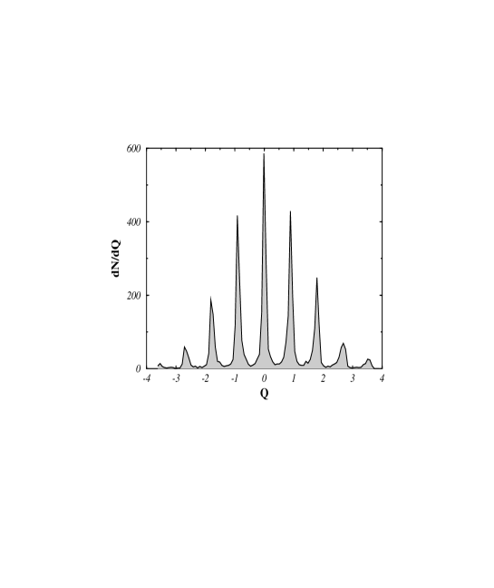
FIG. 7.: Distribution of topological charges for an ensemble of 5000 thermalized configurations in pure gauge $SU(3)$ at $\beta=6.1$, from [ADD_96] .

The tunneling rate can now be estimated using the following simple idea. If the non-perturbative fields contributing to the gluon condensate are dominated by (weakly interacting) instantons, the condensate is simply proportional to their density, because every single instanton contributes a finite amount $\int d^{4}x(G^{a}_{\mu\nu})^{2}=32\pi^{2}$. Therefore, the value of the gluon condensate provides an upper limit for the instanton density

$$n = {dN_{I+A}\over d^{4}x}\;\leq\;\frac{1}{32\pi^{2}}\langle(G^{a}_{\mu\nu})^{2}\rangle\;\simeq\;1\,{\rm fm}^{-4}.$$ (123)

Another estimate of the instanton density can be obtained from the topological susceptibility. This quantity measures fluctuations of the topological charge in a 4-volume $V$,

$$\chi_{top} = \lim_{V\rightarrow\infty}\frac{\langle Q^{2}\rangle}{V}.$$ (124)

On average, the topological charge vanishes, $\langle Q\rangle=0$, but in a given configuration $Q\neq 0$ in general (see Fig. 7). Topological fluctuations provide an important characteristic of the vacuum in pure gauge QCD. However, in the presence of massless quarks, the topological charge is screened and $\chi_{top}=0$ (see Sec. V E). The value of $\chi_{top}$ in quenched QCD can be estimated using the Witten-Veneziano relation (115)

$$\chi_{top} = \frac{f^{2}_{\pi}}{2N_{F}}\left(m^{2}_{\eta}+m^{2}_{\eta^{\prime}}-2m^{2}_{K}\right)\;=\;(180\,{\rm MeV})^{4}.$$ (125)

If one assumes that instantons and anti-instantons are uncorrelated, the topological susceptibility can be estimated as follows. The topological charge in some volume $V$ is $Q=N_{I}-N_{A}$. For a system with Poissonian statistics, the fluctuations in the particle numbers are $\Delta N_{I,A}\simeq\sqrt{N_{I,A}}$. This means that for a random system of instantons, we expect $\chi_{top}=N/V$. Using the phenomenological estimate from above, we again get $(N/V)\simeq 1\,{\rm fm}^{-4}$.

How reliable are these estimates? Both methods suffer from uncertainties that are hard to assess. For the gluon condensate, there is no systematic method to separate perturbative and non-perturbative contributions. The sum rule method effectively determines contributions to the gluon condensate with momenta below a certain separation scale. This corresponds to instanton fluctuations above a given size. This in itself is not a problem, since the rate of small instantons can be determined perturbatively, but the value of the separation scale ($\mu\sim 1\,{rmGeV}$) is not very well determined. In any case, the connection of the gluon condensate with instantons is indirect, other fluctuations might very well play a role. The estimate of the instanton density from the (quenched) topological susceptibility relies on the assumption that instantons are distributed randomly. In the presence of light quarks, this assumption is certainly incorrect (that is why an extrapolation from quenched to real QCD is necessary).

B The typical instanton size and the instanton liquid model

Next to the tunneling rate, the typical instanton size is the most important parameter characterizing the instanton ensemble. If instantons are too large, it does not make any sense to speak of individual tunneling events and semi-classical theory is inapplicable. If instantons are too small, then semi-classical theory is good, but the tunneling rate is strongly suppressed. The first estimate of the typical instanton size was also made in [SVZ_78], based on the estimate of the tunneling rate given above.

If the total tunneling rate can be calculated from the semi-classical ’t Hooft formula, we can ask up to what critical size we have to integrate the rate in order to get the phenomenological instanton density

$$\int_{0}^{\rho_{max}}d\rho\,n_{0}(\rho) = n_{phen}$$ (126)

Using $n_{phen}=1\,{\rm fm}^{-4}$, Shifman et al. concluded that $\rho_{max}\simeq 1\,{\rm fm}$. This is a very pessimistic result, because it implies that the instanton action is not large, so the semi-classical approximation is useless. Also, if instantons are that large, they overlap strongly and it makes no sense to speak of individual instantons.

There are two possible ways in which the semi-classical approximation can break down as the typical size becomes large. One possibility is that (higher loop) perturbative fluctuations start to grow. We have discussed these effects in the double well potential (see Sec. II A 4), but in gauge theory, the two-loop ($O(1/S_{0})$) corrections to the semi-classical result are not yet known. Another possibility is that non-perturbative (multi instanton etc.) effects become important. These effects can be estimated from the gluon condensate. The interaction of an instanton with an arbitrary weak external field $G^{a\,ext}_{\mu\nu}$ is given by (see Sec. IV A 1)

$$S_{int} = {2\pi^{2}\rho^{2}\over g^{2}}\bar{\eta}^{a}_{\mu\nu}U^{ab}G^{b\,ext}_{\mu\nu}$$ (127)

where $U$ is the matrix that describes the instanton orientation in color space. This is a dipole interaction, so to first order it does not contribute to the average action. To second order in $G^{a\,ext}_{\mu\nu}$, one has [SVZ_80]

$$n(\rho) = n_{0}(\rho)\left[1+\frac{\pi^{4}\rho^{4}}{2g^{4}}\langle(G^{a}_{\mu\nu})^{2}\rangle+\ldots\right].$$ (128)

From the knowledge of the gluon condensate we can now estimate for what size non-perturbative effects become important. Using the SVZ value, we see that for $\rho>0.2$ fm the interaction with vacuum fields (of whatever origin) is not negligible. Unfortunately, for $\rho<0.2$ fm the total density of instantons is too small as compared to the phenomenological estimate.

However, it is important to note the sign of the correction. The non-perturbative contribution leads to a tunneling rate that grows even faster than the semi-classical rate. Accounting for higher order effects by exponentiating the second order contribution, [Shu_82] suggested to estimate the critical size from the modified condition

$$\int_{0}^{\rho_{max}}d\rho\,n_{0}(\rho)\exp\left[\frac{\pi^{4}\rho^{4}}{2g^{4}}\langle(G_{a\mu\nu})^{2}\rangle\right] = n_{phen}.$$ (129)

Since the rate grows faster, the critical size is shifted to a smaller value

$$\rho_{max} \sim 1/3\,{\rm fm}.$$ (130)

If the typical instanton is indeed small, we obtain a completely different perspective on the QCD vacuum:

1. Since the instanton size is significantly smaller than the typical separation $R$ between instantons, $\rho/R\sim 1/3$, the vacuum is fairly dilute. The fraction of spacetime occupied by strong fields is only a few per cent.

2. The fields inside the instanton are very strong, $G_{\mu\nu}\gg\Lambda^{2}$. This means that the semi-classical approximation is valid, and the typical action is large

   $$S_{0}=8\pi^{2}/g^{2}(\rho)\sim 10-15\gg 1.$$ (131)

   Higher order corrections are proportional to $1/S_{0}$ and presumably small.

3. Instantons retain their individuality and are not destroyed by interactions. From the dipole formula, one can estimate

   $$|\delta S_{int}|\sim(2-3)\ll S_{0}.$$ (132)

4. Nevertheless, interactions are important for the structure of the instanton ensemble, since

   $$\exp|\delta S_{int}|\sim 20\gg 1.$$ (133)

   This implies that interaction have a significant effect on correlations among instantons, the instanton ensemble in QCD is not a dilute gas, but an interacting liquid.

Improved estimates of the instanton size can be obtained from phenomenological applications of instantons. The average instanton size determines the structure of chiral symmetry breaking, in particular the values of the quark condensate, the pion mass, its decay constant and its form factor. We will discuss these observables in more detail in the next sections.

In particular, the consequences of the vacuum structure advocated here were studied in the context of the “Random Instanton Liquid Model” (RILM). The idea is to fix $N/V=1\,{\rm fm}^{-4}$ and $\rho=1/3$ fm and add the assumption that the distribution of instanton positions as well as color orientations is completely random. This is not necessarily in contradiction with the observation (133) that interactions are important, as long as they do not induce strong correlations among instantons. The random model is sufficiently simple that one can study a large number of hadronic observables. The agreement with experimental results is quite impressive, thus providing support for the underlying parameters.

C Instantons on the lattice

1 The topological charge and susceptibility

The most direct way to determine the parameters of the instanton liquid is provided by numerical simulations on the lattice. Before we come to direct instantons searches, we would like to discuss the determination of the topological susceptibility, which requires measurements of the total topological charge inside a given volume. This has become a very technical subject, and we will not be able to go into much detail (see the nice, albeit somewhat dated review [Kro_88]). The standard techniques used to evaluate the topological charge are the (i) (naive) field-theoretical, (ii) geometrical and (iii) fermionic methods. Today, these methods are usually used in conjunction with various improvements, like cooling, blocking or improved actions.

The field theoretic method is based on the naive lattice discretization of the topological charge density $G\tilde{G}\sim\epsilon_{\mu\nu\rho\sigma}{\rm tr}[U_{\mu\nu}U_{\rho\sigma}]$, where $U_{\mu\nu}$ is the elementary plaquette in the $\mu\nu$ plane. The method is simple to implement, but it has no topological meaning and the naive topological charge $Q$ is not even an integer. In addition to that, the topological susceptibility suffers from large renormalization effects and mixes with other operators, in particular the unit operator and the gluon condensate [CDP_88].

There are a number of “geometric” algorithms, that ensure that $Q$ has topological significance [Lue_82, Woi_83, PS_86]. This means that $Q$ is always an integer and that the topological charge can be expressed as a surface integral. All these methods are based on fixing the gauge and using some interpolation procedure to reconstruct a smooth gauge potential from the discrete lattice data. For a finite lattice with the topology of a 4-dimensional torus, the topology of the gauge fields resides in the transition functions that connect the gauge potential on the boundaries. The geometric method provides a well defined topological charge for almost all gauge configurations. In the continuum, different topological sectors are separated by configurations with infinite action. On the lattice however, different sectors are separated by exceptional finite action configurations called dislocations. Although expected to be unimportant for sufficiently smooth fields, dislocations may spoil the continuum limit on the lattice [PT_89].

Fermionic methods for calculating the topological charge rely on the connection between instantons and fermionic zero modes. Exceptionally small eigenvalues of the Dirac operator on the lattice have been identified [SV_87b, SV_88, LSV_90]. Furthermore, it was demonstrated that the corresponding Dirac eigenvectors have the correct chirality and are spatially correlated with instantons. Fermionic methods are not sensitive to dislocations, but they suffer from problems connected with the difficulty of defining chiral fermions on the lattice. In particular, the (almost) zero-modes connected with instantons are not exactly chiral and the topological charge defined through a fermionic expectation value does suffer from renormalization (for both Wilson and staggered fermions). For this reason, fermionic methods have never been pursued very vigorously (see [Vin_88] for a rare exception). Recently, some progress in constructing chiral fermions on the lattice has been made, see for example [Kap_92, NN_95]. These methods may provide improved measurements of the topological susceptibility [NV_97].

Since most of the difficulties with the field theoretical and geometrical algorithms are related to fluctuations on very short scales, it is natural to supplement these algorithms with some sort of smoothing procedure. The simplest method of this type is cooling [Hoe_86, HTW_87]. In the cooling method, one locally minimizes the action. This operation quickly eliminates short range quantum fluctuations and eventually leads to a smooth configuration, corresponding to the classical content of the original field. It has been verified that these configurations are indeed dominated by instantons [HTW_87, CGHN_94]. It has also been checked that in the cooled configurations, the field-theoretic definition of the topological charge agrees with the more sophisticated, geometrical methods [Wie_90, AGG_90]. Unfortunately, the cooling method also suffers from systematic uncertainties. If the simplest Wilson action is used, instantons gradually shrink and finally fall through the lattice. Improved lattice actions can make instantons stable [FGS_95], but instanton-anti-instanton pairs still annihilate during the cooling process.

The study of topological objects on the lattice is part of a larger effort to find improved or even “perfect” lattice actions and operators. An example for such a method is the “inverse blocking” procedure considered in [HDZ_96]. From the field configuration on the original coarse lattice, one constructs a smoother configuration on a finer lattice by an approximate inverse renormalization group transformation. The method has the advantage that it gives a larger action for dislocations than the standard Wilson action does, thus suppressing undesirable contributions to the topological charge. First tests of improved topological charges are very promising, correctly recovering instantons with sizes as small as $0.8a$. Significantly improved values for the topological susceptibility will hopefully be forthcoming.

Whatever method is used to define $Q$ and measure the topological susceptibility on the lattice, one has to test the behavior of $\chi_{top}$ as the lattice spacing is taken to zero, $a\rightarrow 0$. If the topological susceptibility is a physical quantity, it has to exhibit scaling towards the continuum limit. In the geometrical method, $Q$ itself is not renormalized, and $\chi_{top}$ is expected to show logarithmic scaling (if it were not for the contribution of dislocations). If the field theoretic method is used, $\chi_{top}$ mixes with the unit operator and the gluon condensate. Early studies of the scaling behavior of $\chi_{top}$ can be found in [Woi_83, ISS_83, FGLS_85]. A more detailed study of scaling and the role of mixing effects (in pure gauge $SU(2)$) was recently performed in [ACG_93]. These authors use “heating” to investigate the effect of fluctuations on classical instanton configurations. As quantum fluctuations are turned on, one can study the renormalization of the topological charge. For comparison, if a configuration with no topology is heated, one is mainly sensitive to mixing. Alles et al. conclude that in their window $\beta=(2/g^{2})=2.45-2.525$ everything scales correctly and that $\chi_{top}=3.5(4)\cdot 10^{5}\Lambda_{L}^{4}\simeq(195\,{\rm MeV})^{4}$ (where we have used $\Lambda_{LAT}=8$ MeV). For comparison, the result from cooling is about 30% larger. This discrepancy gives a rough estimate of the uncertainty in the calculation.

FIG. 8.: Scaling test of the topological susceptibility in pure gauge $SU(3)$, from [ADD_96]. The improvement from $Q^{(0)}_{L}$ to $Q^{(2)}_{L}$ is clearly visible. Inside errors, the results are independent on the bare charge $\beta=6/g^{2}$.

An example for the use of an improved topological charge operator is shown in figs. 7 and 8. Figure 7 shows the distribution of topological charges in pure gauge $SU(3)$. As expected, the distribution is a Gaussian with zero mean. A scaling test of the topological susceptibility is shown in Fig. 8. The result clearly shows the reduction in the statistical error achieved using the improved operator and the quality of the scaling behavior. The topological susceptibility is $\chi_{top}=(175(5)\,{\rm MeV})^{4}$. On the other hand, the geometric method (and preliminary results from inverse blocking) gives larger values, for example $\chi_{top}=(260\,{\rm MeV})^{4}$ in pure gauge $SU(3)$ simulations [GG_94]. We conclude that lattice determinations are consistent with the phenomenological value of $\chi_{top}$, but that the uncertainty is still rather large. Also, the scaling behavior of the topological susceptibility extracted from improved (perfect) operators or fermionic definitions still needs to be established in more detail.

A byproduct of the measurements of Alles et al. is a new determination of the gluon condensate in pure gauge $SU(2)$

$$\langle G^{2}\rangle = (4\pi^{2})\cdot 0.38(6)\cdot 10^{8}\Lambda_{L}^{4}\;\simeq\;(1.5\,{\rm GeV})^{4}.$$ (134)

This number is significantly larger than the SVZ value given in the last section, but it is consistent with other lattice data, for example [CGG_89]. However, when comparing the lattice data to the SVZ estimate one should keep in mind that the two results are based on very different physical observables. While the SVZ value is based on the OPE of a hadronic correlator and the value of the separation scale is fairly well determined, lattice results are typically based on the value of the average plaquette and the separation scale is not very well defined.

2 The instanton liquid on the lattice

The topological susceptibility only provides a global characterization of the instanton ensemble. In addition to that, we would also like to identify individual instantons and study their properties. This is true in particular for theories with light quarks, where the total charge is suppressed because of screening effect (see Sec. V E).

Most studies of instantons on the lattice are based on the cooling method. As already mentioned, cooling is not an ideal method for this purpose, because instantons and anti-instantons annihilate during cooling. While this process does not affect the total charge, it does affect the density of instantons and anti-instantons. Ultimately, improved operators are certainly the method of choice. Nevertheless, cooling has the advantage of providing smooth gauge configurations that are easily interpreted in terms of continuum fields.

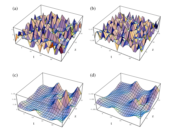
FIG. 9.: A typical slice through a lattice configuration before (a,b) and after 25 cooling sweeps (c,d), from [CGHN_94]. Figs. (a,c) show the fields strength $G^{2}$ and Figs. (b,d) the topological charge density $G\tilde{G}$. The lattice units are $a=0.16$ fm before and $a=0.14$ fm after 25 cooling sweeps.

A typical field configuration after the quantum noise has disappeared is shown in Fig. 9 [CGHN_94]. The left panel shows the field strength on a slice through the lattice. One can clearly identify individual classical objects. The right panel shows the distribution of the topological charge, demonstrating that the classical configurations are indeed instantons and anti-instantons. Fixing physical units from the (quenched) rho meson mass, Chu et al. conclude that the instanton density in pure gauge QCD is $(1.3-1.6)\,{\rm fm}^{-4}$. This number is indeed close to the estimate presented above.

The next question concerns the average size of an instanton. A qualitative confirmation of the instanton liquid value $\rho\sim 1/3\,{\rm fm}$ was first obtained by [PV_88]. More quantitative measurements [CGHN_94] are based on fitting of the topological charge correlation function after cooling. The fit is very good and gives an average size $\rho=0.35fm$.

FIG. 10.: Instanton size distribution in purge gauge $SU(2)$, from [MS_95, Shu_95]. The size $\rho$ is given in $fm$, where lattice units have been fixed from the glueball mass $m_{0^{++}}=1.7$ GeV. Solid squares and dots correspond to $16^{4},\,4/g^{2}=2.4$ and $24^{4},\,4/g^{2}=2.5$, respectively (the dotted and dashed lines simply serve to guide the eye). The open points come from an interacting instanton calculation, while the solid curve corresponds to the parameterization discussed in the text.

More detail is provided by measurements of the instanton size distribution. Lattice studies of this type were recently performed for purge gauge $SU(2)$ by [MS_95] and [FPS_97]. The results obtained by Michael and Spencer on two different size lattices are shown in Fig. 10(a). The agreement between the two measurements is best for large instantons, while it is not so good for small $\rho$. That is of course exactly as expected; instantons of size $\rho\sim a$ fall through the lattice during cooling. The most important result is the existence of a relatively sharp maximum in the size distribution together with a strong suppression of large-size instantons. The physical mechanism for this effect is still not adequately understood. In Fig. 10 we compare the lattice data with an instanton liquid calculation, where large instantons are suppressed by a repulsive core in the instanton interaction [Shu_95].

FIG. 11.: The distribution of the separation of like and unlike instanton pairs in pure gauge $SU(2)$, from [MS_95]. The distance to the closest neighbor (after cooling) is given in lattice units $a\simeq 0.08$ fm.

In addition to the size distribution, [MS_95] also studied correlations among instantons. They find that, on average, unlike pairs are closer than like pairs, $\langle R(IA)\rangle\simeq 0.7\langle R(II)\rangle$. This clearly suggests an attractive interaction between instantons and anti-instantons. The distribution of pseudo-particle separations is shown in Fig. 11. There are very few IA-pairs with very small separation, because these pairs easily annihilate during cooling. Like pairs show an enhancement at small $R$, a feature which is not understood at present.

After identifying instantons on the lattice, the next step is to study the importance of instantons for physical observables. We will discuss an example for this line of research in Sec. VI E, where we present hadronic correlation functions in cooled configurations. Another example can be found in [FMT_97], which shows that there is a strong correlation between the quark condensate and the location of instantons after cooling.

3 The fate of large-size instantons and the beta function

We have seen that both phenomenology and the available lattice data suggest that instantons larger than $\rho\simeq 1/3$ fm are strongly suppressed in QCD. In Sec. II C 4 we saw that this result can not be understood from the leading order semi-classical formula. This leaves essentially three possibilities: The instanton distribution is regulated by higher order quantum effects, by classical instanton interactions, or by the interaction of instantons with other classical objects (e.g. monopoles or strings).

The possible role of repulsive interactions between instantons will be discussed in Sec. IV (this is also what the open dots in Fig. 10 are based on). It is hard to speculate on the role of other classical fields, although we will try to summarize some work in this direction in the next section. Here, we would like to discuss the possibility that the size distribution is regulated by quantum fluctuations [Shu_95]. If this is the case, gross features of the size distribution can be studies by considering a single instanton rather than an interacting ensemble.

The Gell-Mann-Low beta function is defined as a derivative of the coupling constant $g$ over the logarithm of the normalization scale $\mu$ at which $g$ is determined

$$\beta(g)=\frac{\partial g}{\partial\log\mu}=-b\frac{g^{3}}{16\pi^{2}}-b^{\prime}\frac{g^{5}}{(16\pi^{2})^{2}}+\ldots$$ (135)

In QCD with $N_{c}$ colors and $N_{f}$ light flavors we have $b=11N_{c}/3-2N_{f}/3$ and $b^{\prime}=34N_{c}^{2}/3-13N_{c}N_{f}/3+N_{f}/N_{c}$. Remember that the tunneling amplitude is $n(\rho)\sim\rho^{-5}\exp[-(8\pi^{2})/g^{2}(\rho)]$. In the weak coupling domain one can use the one-loop running coupling and $n(\rho)\sim\rho^{b-5}\Lambda^{b}$. This means that the strong growth of the size distribution in QCD is related to the large value of $b\simeq 9$.

For pedagogical reasons, we would like to start our discussion in the domain of the phase diagram where $b$ is small and this dangerous phenomenon is absent. For $N_{c}=3$ colors, $b$ is zero if $N_{f}=33/2\simeq 16$. When $b$ is small and positive, it turns out that the next coefficient $b^{\prime}$ is negative [BM_74, BZ_82] and therefore beta function has a zero at

$$\frac{g^{2}_{*}}{16\pi^{2}}=-\frac{b}{b^{\prime}}.$$ (136)

Since $b$ is small, so is $g_{*}$, and the perturbative calculation is reliable. If the beta function has a zero, the coupling constant will first grow as one goes to larger distances but then stop running (“freeze”) as the critical value $g_{*}$ is approached. In this case, the large distance behavior of all correlation functions is governed by the infrared fixed point and the correlators decay as fractional powers of the distance. In this domain the instanton contribution to the partition function is of the order $\exp(-16\pi^{2}/g^{2}_{*})\sim\exp(-|b^{\prime}/b|)$, so it is exponentially small if $b$ is small.

What happens if $N_{f}$ is reduced, so that we move away from the $b=0$ line? The infrared fixed point survives in some domain (the conformal region), but the value of the critical coupling grows. Eventually, non-perturbative effects (instantons in particular) grow exponentially and the perturbative result (136) is unreliable. As we will discuss in Sec. IX D, existing lattice data suggests that the boundary of the conformal domain is around $N_{f}=7$ for $N_{c}=3$ [IKK_96].

There is no unique way to define the beta function in the non-perturbative regime. In our context, a preferred definition is provided by the value of instanton action $S_{inst}=8\pi^{2}/g^{2}(\rho)$ as a function of the instanton size. This quantity can be studied directly on the lattice by heating (i.e. adding quantum fluctuations) a smooth instanton of given size. This program is not yet implemented, but one can get some input from the measured instanton size distribution. If $S_{inst}\gg 1$, the semiclassical expression $n(\rho)\sim\rho^{-5}\exp(-S_{inst})$ should be valid and we can extract the effective charge from the measured size distribution.

We have already discussed lattice measurements of $n(\rho)$ in Sec. III B. These results are well reproduced using the semi-classical size distribution with a modified running coupling constant [Shu_95]

$$\frac{8\pi^{2}}{g^{2}(\rho)} = bL+\frac{b^{\prime}}{b}\log L,$$ (137)

where (for $N_{f}=0$) the coefficients are $b=11N_{c}/3,\,b^{\prime}=17N_{c}^{2}/3$ as usual, but the logarithm is regularized according to

$$L = \frac{1}{p}\log\left[\left(\frac{1}{\rho\Lambda}\right)^{p}+C^{p}\right].$$ (138)

For small $\rho$, Eq.(137) reduces to the perturbative running coupling, but for large $\rho$ the coupling stops to run in a manner controlled by the two parameters $C$ and $p$. A good description of the measured size distribution can be obtained with $\Lambda=0.66\,{\rm fm}^{-1},\,p=3.5,\,C=4.8$, shown by the solid line in Fig. 10. In real QCD, the coupling cannot freeze, because the theory has certainly no infrared fixed point. Nevertheless, in order to make the instanton density convergent one does not need the beta function to vanish. It is sufficient that the coupling constant runs more slowly, with an effective $b<5$.

There are some indications from lattice simulations that this is indeed the case, and that there is a consistent trend from $N_{f}=0$ to $N_{f}=16$. These results are based on a definition of the non-perturbative beta function based on pre-asymptotic scaling of hadronic observables. The idea is the following: Ideally, the lattice scale is determined by performing simulations at different couplings $g$, fixing the scale $a$ from the asymptotic (perturbative) relation $g(a)$. Scaling behavior is established by studying many different hadronic observables. Although asymptotic scaling is often violated, a weaker form of scaling might still be present. In this case, the lattice scale $a$ at a given coupling $g$ is determined by measuring a hadronic observable in units of $a$ and then fixing $a$ to give the correct experimental value. This procedure makes sense as long as the result is universal (independent of the observable). Performing simulations at different $g$, one can determine the function $g(a)$ and the beta function.

FIG. 12.: Non-perturbative beta function from $SU(3)$ lattice gauge theory with Wilson action. Open points are from [Gup_92b], solid points from [BKT_95]. The solid line shows the fit discussed in the text.

Lattice results for both pure gauge [Gup_92b] (open points) and $N_{f}=2$ [BKT_95] $SU(3)$ are shown in Fig. 12. In order to compare different theories, it is convenient to normalize the beta function to its asymptotic ($g\rightarrow 0$) value. The ratio

$$R_{\beta}(g) = \frac{d(1/g^{2})}{d\log(a)}\left(\left.\frac{d(1/g^{2})}{d\log(a)}\right|_{g\to 0}\right)^{-1}$$ (139)

tends to 1 as $g\to 0$ ($6/g^{2}\to\infty$). The two-loop correction is positive, so $R_{\beta}\to 1$ from above. However, in the non-perturbative region the results show the opposite trend, with $R_{\beta}$ dropping significantly below 1 around $(6/g^{2})\simeq 6$. This means that the coupling constant runs slower than the one-loop formula suggests. At somewhat smaller $6/g^{2}$, $R_{\beta}$ displays a rapid upward turn which is known as the transition to the strong coupling regime. This part of the data is clearly dominated by lattice artefacts. The significant reduction of the beta function (by about 50%) observed for intermediate values of $g$ is precisely what is is needed to explain the suppression of large size instantons. Furthermore, the reduction of $R_{\beta}$ is even larger for $N_{f}=2$. This might very well be a precursor of the infrared fixed point. At some critical $N_{f}$ we expect $R_{\beta}$ to touch zero. As $N_{f}$ is further increased, the zero should move to weaker coupling (to the right) and reach infinity at $N_{f}=33/2$.

D Instantons and confinement

After the discovery of instantons, it was hoped that instantons might help to understand confinement in QCD. This hope was mainly inspired by Polyakov’s proof that instantons lead to confinement in 3 dimensional compact QED [Pol_87]). However, there are important difference between 3 and 4 dimensional theories. In 3 dimensions, the field of an instanton looks like a magnetic monopole (with $B\sim 1/r^{2}$), while in 4 dimensions it is a dipole field which falls off as $1/r^{4}$.

For a random ensemble of instantons one can calculate the instanton contribution to the heavy quark potential. In the dilute gas approximation the result is determined by the Wilson loop in the field of an individual instanton [CDG_78b]. The corresponding potential is $V\sim x^{2}$ for small $x$, but tends to a constant at large distances. This result was confirmed by numerical simulations in the random ensemble [Shu_89], as well as the mean field approximation [DPP_89]. The main instanton effect is a renormalization of the heavy quark mass $\delta M_{Q}=50-70MeV$. The force $|dV/dx|$, peaks at $x\simeq 0.5$ fm, but even at this point it is almost an order of magnitude smaller than the string tension [Shu_89].

Later attempts to explain confinement in terms of instantons (or similar objects) fall roughly into three different categories: objects with fractional topological charge, strongly correlated instantons and the effects of very large instantons.

Classical objects with fractional topological charge were first seriously considered in [CDG_78], which proposed a liquid consisting of instantons and merons. Merons are singular configurations with topological charge $Q=1/2$ [AFF_76]. Basically, one can interpret merons as the result of splitting the dipole field of an instanton into two halves. This means that merons have long-range fields.

Another way to introduce fractional charge is by considering twisted boundary conditions [tHo_81b]. In this case, one finds fracton solutions (also known as ’t Hooft fluxes) with topological charges quantized in units $1/N_{c}$. Gonzales-Arroyo and Martinez suggested that confinement is produced by an ensemble of these objects glued together [GAM_96]. In order to study this hypothesis, they measured the string tension in cooled and uncooled configurations with twisted boundary conditions. They find that fractionally charged objects can indeed be identified and that their number roughly scales with the string tension. Clearly, there are many problems that need to be understood, in particular what the role of the boundary condition is and how regions with twisted boundary conditions can be glued together.

An important attempt at understanding confinement is based on the role of magnetic monopoles (see below). One can make monopole-like configuration (more precisely, dyon-like, since the fields are self-dual) from instantons by lining up identically oriented instantons. Another possibility is a chain of strongly correlated instanton-anti-instanton pairs which might create an infinitely long monopole loop. Under normal circumstances, however, these objects have very small entropy and they are not found in the simulations discussed in Sec. V.

The possible role of very large instantons was discussed in [DP_96]. These authors propose that instantons can cause confinement if the size distribution behaves as $n(\rho)\sim 1/\rho^{3}$. This can be understood as follows. In Sec. IV H, we will show that the mass renormalization of a heavy quark due to instantons is $\Delta M_{Q}\sim(N/V)\rho^{3}$. For typical instanton radii this contribution is not very important, but if the size distribution has a $1/\rho^{3}$ tail, then $\Delta M_{Q}$ is linearly divergent, a possible signature of confinement. This is very intriguing, but again, there are a number of open questions. For one, the $1/\rho^{3}$ distribution implies that the total volume occupied by instantons is infinite. Also, very large instantons would introduce long range correlations which are inconsistent with the expected exponential decay of gluonic correlation functions.

FIG. 13.: Squared topological charge density around a static heavy quark-anti-quark pair in $SU(3)$ with $N_{f}=3$, from [FMO_95]. The results were obtained on an $8^{3}\times 4$ at $6/g^{2}=5.6$. The topological charge was measured after 5 cooling steps.

Whatever the mechanism of confinement may turn out to be, it is clear that instantons should be affected by confinement is some way. One example for this line of reasoning is the idea that confinement might be the reason for the suppression of large size instantons. A related, more phenomenological suggestion is that instantons provide a dynamical mechanism for bag formation, see [Shu_78, CDG_79]. A lattice measurement of the suppression of instantons in the field of a static quark was recently performed by the Vienna group (see [FMO_95] and references therein). The measured distribution of the topological charge is shown in Fig. 13. The instanton density around the static charge is indeed significantly suppressed, by about a factor of two. Since instantons give a vacuum energy density on the order of $-1\,{\rm GeV/fm}^{3}$, this effect alone generates a significant difference in the non-perturbative energy density (bag constant) inside and outside of a hadron.

A very interesting picture of confinement in QCD is based on the idea that the QCD vacuum behaves like a dual superconductor, formed by the condensation of magnetic monopoles [Man_76]. Although the details of this mechanism lead to many serious questions [DFGO], there is some evidence in favor of this scenario from lattice simulations. There are no semi-classical monopole solutions in QCD, but monopoles can arise as singularities after imposing a gauge condition [tHo_81]. The number and the location of monopole trajectories will then depend on the gauge choice. In practice, the so called maximal abelian gauge (MAG) has turned out to be particularly useful [KSW_87]. The MAG is specified by the condition that the norm of the off-diagonal components of the gauge fields are minimal, e.g. ${\rm tr}((A\mu^{1})^{2}+(A_{\mu}^{2})^{2})={\rm min}$ in $SU(2)$. This leaves one $U(1)$ degree of freedom unfixed, so in this preferred subgroup one can identify magnetic charges, study their trajectories and evaluate their contribution to the (abelian) string tension. The key observation is that the abelian string tension (in MAG) is numerically close to the full non-abelian string tension, and that it is dominated by the longest monopole loops [SS_89, Suz_93].

We can certainly not go into details of these calculations, which would require a review in itself, but only mention some ideas how instantons and monopoles might be correlated. If monopoles are responsible for color confinement, then their paths should wind around the color flux tubes, just like electric current lines wind around magnetic flux tubes in ordinary superconductors. We have already mentioned that color flux tubes expel topological charges, see Fig. 13. This suggests that instantons and monopoles should be (anti?) correlated. Lattice simulations that combine abelian projection with the cooling technique or improved topological charges have indeed observed a strong positive correlation between monopoles and instantons [FMT_97b]. In order to understand this phenomenon in more detail, a number of authors have studied monopole trajectories associated with individual instantons or instanton pairs [HT_95, SIT_95, CG_95]. It was observed that each instanton is associated with a monopole loop. For instanton-anti-instanton pairs, these loops may either form two separate or one common loop, depending on the relative color orientation of the two instantons. In the mean time it was shown that the small loops associated with individual instantons do not correspond to global minima of the gauge fixing functional and should be discarded [BOT_96]. On the other hand, monopole trajectories connecting two or more instantons appear to be physical. The main physical question is then whether these monopole loops can percolate to form the long monopole loops responsible for confinement.

IV Towards a theory of the instanton ensemble

A The instanton interaction

1 The gauge interaction

In the last chapter we argued that the density of instantons in the QCD vacuum is quite significant, implying that interactions among them are essential in understanding the instanton ensemble. In general, it is clear that field configurations containing both instanton and anti-instantons are not exact solutions of the equations of motion and that the action of an instanton anti-instanton pair is not equal to twice the single instanton action. The interaction is defined by

$$S_{int} = S(A_{\mu}^{IA})-2S_{0},$$ (140)

where $A_{\mu}^{IA}$ is the gauge potential of the instanton-anti-instanton pair. Since $A_{\mu}^{IA}$ is not an exact solution, there is some freedom in choosing an ansatz for the gauge field. This freedom corresponds to finding a convenient parametrization of the field configurations in the vicinity of an approximate saddle point. In general, we have to integrate over all field configurations anyway, but the ansatz determines the way we split coordinates into approximate zero modes and non-zero modes.

For well separated IA pairs, the fields are not strongly distorted and the interaction is well defined. For very close pairs, on the other hand, the fields are strongly modified and the interaction is not well determined. In addition to that, if the instanton and anti-instanton begin to annihilate, the gauge fields become perturbative and should not be included in semi-classical approximations. We will comment on the present understanding of these questions below.

The interaction between instantons at large distances was derived by Callan, Dashen and Gross [CDG_78] (see also [For_77]). They began by studying the interaction of an instanton with a weak, slowly varying external field $(G^{a}_{\mu\nu})_{ext}$. In order ensure that the gauge field is localized, the instanton is put in the singular gauge. One then finds

$$S_{int} = -\frac{2\pi^{2}}{g^{2}}\rho^{2}\bar{\eta}^{a}_{\mu\nu}(G^{a}_{\mu\nu})_{ext}.$$ (141)

This result can be interpreted as the external field interacting with the color magnetic “dipole moment” $\frac{2\pi^{2}}{g^{2}}\rho^{2}\bar{\eta}^{a}_{\mu\nu}$ of the instanton. Note that the interaction vanishes if the external field is self-dual. If the external field is taken to be an anti-instanton at distance $R$, the interaction is

$$S_{int} = \frac{32\pi^{2}}{g^{2}}\rho_{I}^{2}\rho_{A}^{2}\bar{\eta}^{a}_{\mu\rho}\eta^{b}_{\nu\rho}R^{ab}\frac{\hat{R}_{\mu}\hat{R}_{\nu}}{R^{4}},$$ (142)

where $R^{ab}$ is the relative color orientation matrix $R^{ab}=\frac{1}{2}{\rm tr}(U\tau^{a}U^{\dagger}\tau^{b})$ and $\hat{R}$ is the unit vector connecting the centers of the instanton and anti-instanton. The dipole-dipole form of the interaction is quite general, the interaction of topological objects in other theories, such as skyrmions or $O(3)$ instantons, is of similar type.

Instead of considering the dipole interaction as a classical phenomenon, we can also look at the interaction as a quantum effect, due to gluon exchanges between the instantons [Zak_92]. The linearized interaction (141) corresponds to an instanton vertex that describes the emission of a gluon from the classical instanton field. The amplitude for the exchange of one gluon between an instanton and an anti-instanton is given by

$$\frac{4\pi^{4}}{g^{2}}\rho_{1}^{2}\rho_{2}^{2}R_{I}^{ab}R_{A}^{cd}\eta^{b}_{\mu\nu}\eta^{d}_{\alpha\beta}\langle G^{a}_{\mu\nu}(x)G^{c}_{\alpha\beta}(0)\rangle,$$ (143)

where $\langle G^{a}_{\mu\nu}(x)G^{c}_{\alpha\beta}(0)\rangle$ is the free gauge field propagator

$$\langle G^{a}_{\mu\nu}(x)G^{c}_{\alpha\beta}(0)\rangle = \frac{2\delta^{ac}}{\pi^{2}x^{6}}(g_{\nu\alpha}x_{\mu}x_{\beta}+g_{\mu\beta}x_{\nu}x_{\alpha}-g_{\nu\beta}x_{\mu}x_{\alpha}-g_{\mu\alpha}x_{\nu}x_{\beta}).$$ (144)

Inserting (144) into (143) gives the dipole interaction to first order. Summing all $n$ gluon exchanges allows one to exponentiate the result and reproduce the full dipole interaction (142).

In order to study this interaction in more detail, it is useful to introduce some additional notation. We can characterize the relative color orientation in terms of the four vector $u_{\mu}=\frac{1}{2i}{\rm tr}(U\tau^{+}_{\mu})$, where $\tau^{+}_{\mu}=(\vec{\tau},-i)$. Note that for the gauge group $SU(2)$, $u_{\mu}$ is a real vector with $u^{2}=1$, whereas for $SU(N>2)$, $u_{\mu}$ is complex and $|u|^{2}\leq 1$. Also note that for $SU(N>2)$, the interaction is completely determined by the upper $2\times 2$ block of the $SU(N)$ matrix $U$. We can define a relative color orientation angle $\theta$ by

$$\cos^{2}\theta = \frac{|u\cdot\hat{R}|^{2}}{|u|^{2}}.$$ (145)

In terms of this angle, the dipole interaction is given by

$$S_{int} = -\frac{32\pi^{2}}{g^{2}}\frac{\rho_{1}^{2}\rho_{2}^{2}}{R^{4}}|u|^{2}\left(1-4\cos^{2}\theta\right).$$ (146)

The orientational factor $d=1-4\cos^{2}\theta$ varies between 1 and $-3$. We also observe that the dipole interaction vanishes upon averaging over all angles $\theta$.

FIG. 14.: a) Classical instanton-anti-instanton interaction in the streamline (dash-dotted) and ratio ansatz (short dashed line). The interaction is given in units of the single instanton action $S_{0}$ for the most attractive ($\cos\theta=1$ and most repulsive ($\cos\theta=0$) orientations. The solid line shows the original stream line interaction supplemented by the core discussed in Sec. V C. b) Fermionic overlap matrix element in the stream line (solid) and ratio ansatz (dotted line). The matrix elements are given in units of the geometric mean of the instanton radii.

The dipole interaction is the leading part of the interaction at large distances. In order to determine the interaction at intermediate separation, we have to evaluate the total action for an IA pair. This is most easily done for the so called sum ansatz

$$A_{\mu}^{IA} = A_{\mu}^{I}+A_{\mu}^{A},$$ (147)

where again both the instanton and the anti-instanton are in the singular gauge. The action $S=\frac{1}{4}\int d^{4}x\,G^{2}$ can easily be split into the free part $2S_{0}$ and the interaction. Systematically expanding in $1/R^{2}$, one finds [DP_84]

$$S^{IA}_{int} = -\frac{8\pi^{2}}{g^{2}}\left\{\left(|u|^{2}-4|u\cdot\hat{R}|^{2}\right)\left[\frac{4\rho_{1}^{2}\rho_{2}^{2}}{R^{4}}-\frac{15\rho_{1}^{2}\rho_{2}^{2}(\rho_{1}^{2}+\rho_{2}^{2})}{2R^{6}}\right]\right.$$ (149)

$$\hskip 56.9055pt+\left.|u|^{2}\frac{9\rho_{1}^{2}\rho_{2}^{2}(\rho_{1}^{2}+\rho_{2}^{2})}{2R^{6}}+O(R^{-8})\right\}$$

for the $IA$ interaction and

$$S^{II}_{int} = \frac{8\pi^{2}}{g^{2}}\left(9+3|u|^{2}-4|\vec{u}|^{2}\right)\frac{\rho_{1}^{2}\rho_{2}^{2}(\rho_{1}^{2}+\rho_{2}^{2})}{2R^{6}}+O(R^{-8})$$ (150)

for the $II$ interaction. Here, $\vec{u}=$ denotes the spatial components of the four-vector $u_{\mu}$. To first order, we find the dipole interaction in the $IA$ channel and no interaction between two instantons. To next order, there is a repulsive interaction for both $IA$ and $II$.

Clearly, it is important to understand to what extent this interaction is unique, or if it depends on details of the underlying ansatz for the gauge potential. It was also realized that the simple sum ansatz leads to certain artefacts, for example that the field strength at the centers of the two instantons becomes infinite and that there is an interaction between pseudo-particles of the same charge. One of us [Shu_88] therefore proposed the “ratio” ansatz

$$A_{\mu}^{a} = \frac{2R_{I}^{ab}\bar{\eta}^{b}_{\mu\nu}\frac{\rho_{I}^{2}(x-z_{I})_{\nu}}{(x-z_{I})^{4}}+2R_{A}^{ab}\eta^{b}_{\mu\nu}\frac{\rho_{A}^{2}(x-z_{A})_{\nu}}{(x-z_{A})^{4}}}{1+\frac{\rho_{I}^{2}}{(x-z_{I})^{2}}+\frac{\rho_{A}^{2}}{(x-z_{A})^{2}}},$$ (151)

whose form was inspired by ’t Hooft’s exact multi-instanton solution. This ansatz ensures that the field strength is regular everywhere and that (at least if they have the same orientation) there is no interaction between pseudo-particles of the same charge. Deriving an analytic expression for the interaction in the ratio ansatz is somewhat tedious. Instead, we have calculated the interaction numerically and parameterized the result, see [SV_91] and Fig. 14. We observe that both the sum and the ratio ansatz lead to the dipole interaction at large distances, but the amount of repulsion at short distance is significantly reduced in the ratio ansatz.

Given these ambiguities, the question is whether one can find the best possible ansatz for the gauge field of an $IA$ pair. This question was answered with the introduction of the streamline or valley method [BY_86]. The basic idea is to start from a well separated instanton-anti-instanton pair, which is an approximate solution of the equations of motion, and then let the system evolve under the force given by the variation of the action [Shu_88c]. For a scalar field theory, the streamline equation is given by

$$f(\lambda)\frac{d\phi}{d\lambda} = \frac{\delta S}{\delta\phi},$$ (152)

where $\lambda$ is the collective variable corresponding to the evolution of the pair and $f(\lambda)$ is a function that depends on the parametrization of the streamline. The initial conditions are $\phi(\infty)=\phi_{c}$ and $\phi^{\prime}(\infty)=\phi_{0}$, where $\phi_{c}$ is the classical solution corresponding to a well separated instanton anti-instanton pair and $\phi_{0}$ is the translational zero mode.

In QCD, the streamline equations were solved by [Ver_91] using the conformal invariance of the classical equations of motion. Conformal invariance implies that an instanton anti-instanton pair in the singular gauge at some distance $R$ is equivalent to a regular gauge instanton and a singular gauge anti-instanton with the same center, but different sizes. We do not want to go into details of the construction, but refer the reader to the original work. It turns out that the resulting gauge configurations are very close to the following ansatz originally proposed by Yung [Yun_88]

$$A_{\mu}^{a} = 2\eta^{a}_{\mu\nu}x_{\nu}\frac{1}{x^{2}+\rho^{2}\lambda}+2R^{ab}\eta^{b}_{\mu\nu}x_{\nu}\frac{\rho^{2}}{\lambda}\frac{1}{x^{2}(x^{2}+\rho^{2}/\lambda)},$$ (153)

where $\rho=\sqrt{\rho_{1}\rho_{2}}$ is the geometric mean of the two instanton radii and $\lambda$ is the conformal parameter

$$\lambda = \frac{R^{2}+\rho_{1}^{2}+\rho_{2}^{2}}{2\rho_{1}\rho_{2}}+\left(\frac{(R^{2}+\rho_{1}^{2}+\rho_{2}^{2})^{2}}{4\rho_{1}^{2}\rho_{2}^{2}}-1\right)^{1/2}.$$ (154)

Note that the conformal parameter is large not only if the instanton-antiinstanton separation $R$ is much bigger than the mean (geometric) size, but also if $R$ is small and one of the instantons is much bigger than the other. This situation is important when we consider the suppression of large-size instantons.

The interaction for this ansatz is given by [Ver_91]

$$S_{IA} = \frac{8\pi^{2}}{g^{2}}\frac{4}{(\lambda^{2}-1)^{3}}\bigg{\{}-4\left(1-\lambda^{4}+4\lambda^{2}\log(\lambda)\right)\left[|u|^{2}-4|u\cdot\hat{R}|^{2}\right]$$ (156)

$$\hskip 28.45274pt\mbox{}+2\left(1-\lambda^{2}+(1+\lambda^{2})\log(\lambda)\right)\left[(|u|^{2}-4|u\cdot\hat{R}|^{2})^{2}+|u|^{4}+2(u)^{2}(u^{*})^{2}\right]\bigg{\}},$$

which is also shown in Fig. 14. For the repulsive orientation, the interaction is similar to the ratio ansatz, and the average interaction is repulsive. For the most attractive orientation, however, the interaction approaches $-2S_{0}$ at short distance, showing that the instanton and anti-instanton annihilate each other and the total action of the pair approaches zero.

It is interesting to note that the Yung ansatz, at least to order $1/R^{6}$, leads to the same interaction as the perturbative method (143) if carried out to higher order [AM_91, BS_93, DP_94]. This problem is related to the calculation of instanton induced processes at high energy (like multi gluon production in QCD, or the baryon number violating cross section in electroweak theory). To leading order in $E/M_{sph}$, where $E$ is the bombarding energy and $M_{sph}$ the sphaleron barrier (see Sec. VIII B), the cross section is given by

$$\sigma_{tot} = {\rm disc}\int d^{4}R\,e^{ip\cdot R}\int\int d\Omega_{1}d\Omega_{2}\,n(\rho_{1})n(\rho_{2})e^{-S_{int}(R,\Omega_{12})},$$ (157)

where $\Omega_{i}=(z_{i},\rho_{i},U_{i})$ are the collective coordinates associated with the instanton and anti-instanton and ${\rm disc}\,f(s)=\frac{1}{2i}(f(s+i\epsilon)-f(s-i\epsilon))$ denotes the discontinuity of the amplitude after continuation to Minkowski space, $s=p^{2}>0$. Given the agreement of the streamline method and the perturbative calculation to leading and next to leading order, it has been suggested to use the behavior of $\sigma_{tot}$ at high energy in order to define the interaction $S_{int}$ [DP_93]. The behavior of this quantity is still debated, but it is generally believed that the baryon number violating cross section does not reach the unitarity bound. In that case, the interaction would have to have some repulsion at short distance, unlike the streamline solution.

Another possibility to make sense of the short distance part of the $IA$ interaction in the streamline method is to use analytic continuation in the coupling constant, as we have discussed in Sec. II A. Allowing $g^{2}\to-g^{2}$ gives a new saddle point in the complex $g$ plane at which the $IA$ interaction is repulsive and the semi-classical method is under control.

2 The fermionic interaction

In the presence of light fermions, instantons interact with each other not only through their gauge fields, but also through fermion exchanges. The basic idea in dealing with the fermionic interaction is that the Dirac spectrum can be split into quasi-zero modes, linear combinations of the zero modes of the individual instantons, and non-zero modes. Here we will focus on the interaction due to approximate zero modes. The interaction due to non-zero modes and the corrections due to interference between zero and non-zero modes were studied in [BC_78, LB_79].

In the basis spanned by the zero modes, we can write the Dirac operator as

$$iD\!\!\!\!/ = \left(\begin{array}[]{cc}0&T_{IA}\\ T_{AI}&0\end{array}\right),$$ (160)

where we have introduced the overlap matrix elements $T_{IA}$

$$T_{IA} = \int d^{4}x\,\psi_{0,I}^{\dagger}(x-z_{I})iD\!\!\!\!/\,\psi_{0,A}(x-z_{A}),$$ (161)

Here, $\psi_{0,I}$ is the fermionic zero mode (110). The matrix elements have the meaning of a hopping amplitude for a quark from one pseudo-particle to another. Indeed, the amplitude for an instanton to emit a quark is given by the amputated zero mode wave function $iD\!\!\!\!/\,\psi_{0,I}$. This shows that the matrix element (161) can be written as two quark-instanton vertices connected by a propagator, $\psi_{0,I}^{\dagger}iD\!\!\!\!/\,(iD\!\!\!\!/\,)^{-1}iD\!\!\!\!/\,\psi_{0,A}$. At large distance, the overlap matrix element decreases as $T_{IA}\sim 1/R^{3}$, which corresponds to the exchange of a massless quark. The determinant of the matrix (160) can be interpreted as the sum of all closed diagrams consisting of (zero mode) quark exchanges between pseudo-particles. In other words, the logarithm of the Dirac operator (160) is the contributions of the ’t Hooft effective interaction to the vacuum energy.

Due to the chirality of the zero modes, the matrix elements $T_{II}$ and $T_{AA}$ between instantons of the same charge vanish. In the sum ansatz, we can use the equations of motion to replace the covariant derivative in (161) by an ordinary one. The dependence on the relative orientation is then given by $T_{IA}=(u\cdot\hat{R})f(R)$. This means that, like the gluonic dipole interaction, the fermion overlap is maximal if $\cos\theta=1$. The matrix element can be parameterized by

$$T_{IA} = i(u\cdot R)\frac{1}{\rho_{I}\rho_{A}}\frac{4.0}{\left(2.0+R^{2}/(\rho_{I}\rho_{A})\right)^{2}}.$$ (162)

A parametrization of the overlap matrix element for the streamline gauge configuration can be found in [SV_92]. The result is compared with the sum ansatz in Fig. 14 (for $\cos\theta=1$). We observe that the matrix elements are very similar at large distance, but differ at short distance.

Using these results, the contribution of an instanton-anti-instanton pair to the partition function may be written as

$$Z_{IA}=V_{4}\int d^{4}zdU\,\exp\left(N_{f}\log|T_{IA}(U,z)|^{2}-S_{int}(U,z)\right).$$ (163)

Here, $z$ is the distance between the centers and $U$ is the relative orientation of the pair. The fermionic part is attractive, while the bosonic part is either attractive or repulsive, depending on the orientation. If the interaction is repulsive, there is a real saddle point for the $z$-integral, whereas for the attractive orientation there is only a saddle point in the complex $z$ plane (as in Sec. II B).

The calculation of the partition function (163) in the saddle point approximation was recently attempted by [SV_97]. They find that for a large number of flavors, $N_{f}>5$, the ground state energy oscillates as a function of $N_{f}$. The period of the oscillation is 4, and the real part of the energy shift vanishes for even $N_{f}=6,8,\ldots$. The reason for these oscillations is exactly the same as in the case of SUSY quantum mechanics: the saddle point gives a complex contribution with a phase that is proportional to the number of flavors.

B Instanton ensembles

In Sec. II C 4 we studied the semi-classical theory of instantons, treating them as very rare (and therefore independent) tunneling events. However, as emphasized in Sec. III A, in QCD instantons are not rare, so one cannot just exponentiate the results obtained for a single instanton. Before we study the instanton ensemble in QCD, we would like to discuss a simple physical analogy. In this picture, we think of instantons as atoms and light quarks as valence electrons.

A system like this can exist in many different phases, e.g. as a gas, liquid or solid. In theories with massless quarks instantons have “unsaturated bonds” and cannot appear individually. Isolated instantons in the form of an atomic gas can only exist if there is a non zero quark mass. The simplest “neutral” object is an instanton-anti-instanton ($IA$) molecule. Therefore, if the instanton density is low (for whatever reason: high temperature, a large Higgs expectation value, etc.) the system should be in a phase consisting of $IA$ molecules. Below, we will also argue that this is the case if the density is not particularly small, but the interactions are strong and favor the formation of molecules, for example if the number of light quarks $N_{f}$ exceeds some critical value. If the instanton ensemble is in the molecular phase, then quarks are bound to molecules and cannot propagate over large distances. This means that there are no eigenmodes with almost zero virtuality, the “conductivity” is zero, or chiral symmetry remains unbroken.

The liquid phase differs from the gas phase in many important respects. The density is determined by the interactions and cannot be arbitrary small. A liquid has a surface tension, etc. As we will see below, the instanton ensemble in QCD has all these properties. In QCD we also expect that chiral symmetry is spontaneously broken. This means that in the ground state, there is a preferred direction in flavor space, characterized by the quark condensate $\langle\bar{q}q\rangle$. This preferred orientation can only be established if quarks form an infinite cluster. In terms of our analogy, this means that electrons are delocalized and the conductivity is non-zero. In the instanton liquid phase, quarks are delocalized because the instanton zero modes become collective.

At very high density, interactions are strong and the ensemble is expected to form a 4-dimensional crystal. In this case, both Lorentz and gauge invariance would be broken spontaneously: clearly, this phase is very different from the QCD vacuum. Fortunately however, explicit calculations [DP_84, SV_90] show that the instanton liquid crystalizes only if the density is pushed to about two orders of magnitude larger than the phenomenological value. At physical densities, the crystaline phase is not favored: although the interaction is attractive, the entropy is too small as compared to the random liquid. The electronic structure of a crystal consists of several bands. In our case, the Fermi surface lies between different bands, so the crystal is an insulator. In QCD, this means that chiral symmetry is not broken.

Another analogy with liquids concerns the question of density stabilization. In order for the system to saturate, we need a short range repulsive force in addition to the attractive long range dipole interaction. We have already mentioned that the nature of the short range interaction and the (possibly related) question of the fate of large instantons in QCD are not well understood. Lattice simulations indicate that large instantons are strongly suppressed, but for the moment we have to include this result in a phenomenological manner.

Let us summarize this qualitative discussion. Depending on the density, the instanton ensemble is expected to be in a gas, liquid or solid phase. The phase boundaries will in general depend on the number of colors and flavors. Large $N_{c}$ favors a crystalline phase, while large $N_{f}$ favors a molecular gas. Both cases are not phenomenologically acceptable as a description of real QCD, with two light and one intermediate mass flavor. We therefore expect (and will show below) that the instanton ensemble in QCD is in the liquid phase.

C The mean field approximation

In order to study the structure of the instanton ensemble in a more quantitative fashion, we consider the partition function for a system of instantons in pure gauge theory

$$Z = \frac{1}{N_{+}!N_{-}!}\prod_{i}^{N_{+}+N_{-}}\int[d\Omega_{i}\,n(\rho_{i})]\,\exp(-S_{int}).$$ (164)

Here, $N_{\pm}$ are the numbers of instantons and anti-instantons, $\Omega_{i}=(z_{i},\rho_{i},U_{i})$ are the collective coordinates of the instanton $i$, $n(\rho)$ is the semi-classical instanton distribution function (102) and $S_{int}$ is the bosonic instanton interaction. In general, the dynamics of a system of pseudo-particles governed by (164) is still quite complicated, so we have to rely on approximation schemes. There are a number of techniques well known from statistical mechanics that can be applied to the problem, for example the mean field approximation or the variational method. These methods are expected to be reliable as long correlations between individual instantons are weak.

The first such attempt was made by Callan, Dashen and Gross [CDG_78]. These authors only included the dipole interaction, which, as we noted above, vanishes on average and produces an attractive interaction to next order in the density. In this case, there is nothing to balance the growth $n(\rho)\sim\rho^{b-5}$ of the semi-classical instanton distribution. In order to deal with this problem, Ilgenfritz and Müller-Preußker [IMP_81] introduced an ad hoc “hard core” in the instanton interaction, see also [Mun_82]. The hard core automatically excludes large instantons and leads to a well behaved partition function. It is important to note that one cannot simply cut the size integration at some $\rho_{c}$, but has to introduce the cutoff in a way that does not violate the conformal invariance of the classical equations of motion. This guarantees that the results do not spoil the renormalization properties of QCD, most notably the trace anomaly (see below). In practice, they chose

$$S_{int} = \left\{\begin{array}[]{cc}\infty&|z_{I}-z_{A}|<(a\rho_{I}^{2}\rho_{A}^{2})^{1/4}\\ 0&|z_{I}-z_{A}|>(a\rho_{I}^{2}\rho_{A}^{2})^{1/4}\end{array}\right.$$ (167)

which leads to an excluded volume in the partition function, controlled by the dimensionless parameter $a$.

We do not go into details of their results, but present the next development [DP_84]. In this work, the arbitrary core is replaced by the interaction in the sum ansatz, see (149,150). The partition function is evaluated using a trial distribution function. If we assume that correlations between instantons are not very important, then a good trial function is given by the product of single instanton distributions $\mu(\rho)$

$$Z_{1} = \frac{1}{N_{+}!N_{-}!}\prod_{i}^{N_{+}+N_{-}}\int d\Omega_{i}\,\mu(\rho_{i})=\frac{1}{N_{+}!N_{-}!}(V\mu_{0})^{N_{+}+N_{-}}$$ (168)

where $\mu_{0}=\int d\rho\,\mu(\rho)$. The distribution $\mu(\rho)$ is determined from the variational principle $\delta\log Z_{1}/\delta\mu=0$. In quantum mechanics a variational wave functions always provides an upper bound on the true ground state energy. The analogous statement in statistical mechanics is known Feynman’s variational principle. Using convexity

$$Z = Z_{1}\langle\exp(-(S-S_{1}))\rangle\;\geq\;Z_{1}\exp(-\langle S-S_{1}\rangle),$$ (169)

where $S_{1}$ is the variational action, one can see that the variational vacuum energy is always higher than the true one.

In our case, the single instanton action is given by $S_{1}=\log(\mu(\rho))$ while $\langle S\rangle$ is the average action calculated from the variational distribution (168). Since the variational ansatz does not include any correlations, only the average interaction enters

$$\langle S_{int}\rangle = \gamma^{2}\rho_{1}^{2}\rho_{2}^{2},\hskip 28.45274pt\gamma^{2}=\frac{27}{4}\frac{N_{c}}{N_{c}^{2}-1}\pi^{2}$$ (170)

for both $IA$ and $II$ pairs. Clearly, (170) is of the same form as the hard core (167) discussed above, only that the dimensionless parameter $\gamma^{2}$ is determined from the interaction in the sum ansatz. Applying the variational principle, one finds [DP_84]

$$\mu(\rho) = n(\rho)\exp\left[-\frac{\beta\gamma^{2}}{V}N\overline{\rho^{2}}\rho^{2}\right],$$ (171)

where $\beta=\beta(\overline{\rho})$ is the average instanton action and $\overline{\rho^{2}}$ is the average size. We observe that the single instanton distribution is cut off at large sizes by the average instanton repulsion. The average size $\overline{\rho^{2}}$ is determined by the self consistency condition $\overline{\rho^{2}}=\mu_{0}^{-1}\int d\rho\mu(\rho)\rho^{2}$. The result is

$$\overline{\rho^{2}} = \left(\frac{\nu V}{\beta\gamma^{2}N}\right)^{1/2},\hskip 28.45274pt\nu=\frac{b-4}{2},$$ (172)

which determines the dimensionless diluteness of the ensemble, $\rho^{4}(N/V)=\nu/(\beta\gamma^{2})$. Using the pure gauge beta function $b=11$, $\gamma^{2}\simeq 25$ from above and $\beta\simeq 15$, we get $\rho^{4}(N/V)=0.01$, even more dilute than phenomenology requires. The instanton density can be fixed from the second self-consistency requirement, $(N/V)=2\mu_{0}$ (the factor 2 comes from instantons and anti-instantons). We get

$$\frac{N}{V} = \Lambda_{PV}^{4}\left[C_{N_{c}}\beta^{2N_{c}}\Gamma(\nu)(\beta\nu\gamma^{2})^{-\nu/2}\right]^{\frac{2}{2+\nu}},$$ (173)

where $C_{N_{c}}$ is the prefactor in Equ. (102). The formula shows that $\Lambda_{PV}$ is the only dimensionful parameter. The final results are

$$\chi_{top}\simeq\frac{N}{V}=(0.65\Lambda_{PV})^{4},\hskip 14.22636pt(\overline{\rho^{2}})^{1/2}=0.47\Lambda_{PV}^{-1}\simeq{1\over 3}R,\hskip 14.22636pt\beta=S_{0}\simeq 15,$$ (174)

consistent with the phenomenological values for $\Lambda_{PV}\simeq 300$ MeV. It is instructive to calculate the free energy as a function of the instanton density. Using $F=-1/V\cdot\log Z$, we have

$$F = \frac{N}{V}\left\{\log\left(\frac{N}{2V\mu_{0}}\right)-\left(1+\frac{\nu}{2}\right)\right\}.$$ (175)

The instanton density is determined by the minimizing the free energy, $\partial F/(\partial(N/V))=0$. The vacuum energy density is given by the value of the free energy at the minimum, $\epsilon=F_{0}$. We find $N/V=2\mu_{0}$ as above and

$$\epsilon = -\frac{b}{4}\left(\frac{N}{V}\right)$$ (176)

Estimating the value of the gluon condensate in a dilute instanton gas, $\langle G^{2}\rangle=32\pi^{2}(N/V)$, we see that (176) is consistent with the trace anomaly. Note that for non-interacting instantons (with the size integration regularized in some fashion), one would expect $\epsilon\simeq-(N/V)$, which is inconsistent with the trace anomaly and shows the importance of respecting classical scale invariance.

The second derivative of the free energy with respect to the instanton density, the compressibility of the instanton liquid, is given by

$$\left.\frac{\partial^{2}F}{\partial(N/V)^{2}}\right|_{n_{0}} = \frac{4}{b}\left(\frac{N}{V}\right),$$ (177)

where $n_{0}$ is the equilibrium density. This observable is also determined by a low energy theorem based on broken scale invariance [NSVZ_81]

$$\int d^{4}x\;\langle G^{2}(0)G^{2}(x)\rangle = (32\pi^{2})\frac{4}{b}\langle G^{2}\rangle.$$ (178)

Here, the left hand side is given by an integral over the field strength correlator, suitably regularized and with the constant disconnected term $\langle G^{2}\rangle^{2}$ subtracted. For a dilute system of instantons, the low energy theorem gives

$$\langle N^{2}\rangle-\langle N\rangle^{2} = \frac{4}{b}\langle N\rangle.$$ (179)

Here, $\langle N\rangle$ is the average number of instantons in a volume $V$. The result (179) shows that density fluctuations in the instanton liquid are not Poissonian. Using the general relation between fluctuations and the compressibility gives the result (177). This means that the form of the free energy near the minimum is determined by the renormalization properties of the theory. Therefore, the functional form (175) is more general than the mean field approximation used to derive it.

How reliable are the numerical results derived from the mean field approximation? The accuracy of the MFA can be checked by doing statistical simulations of the full partition function. We will come to this approach in Sec. V). The other question concerns the accuracy of the sum ansatz. This can be checked explicitly by calculating the induced current $j_{\mu}=D_{\mu}G^{cl}_{\mu\nu}$ in the classical gauge configurations [Shu_85]. This current measures the failure of the gauge potential to be a true saddle point. In the sum ansatz, the induced current gives a sizeable contribution to the action which means that this ansatz is not a good starting point for a self-consistent solution.

In principle, this problem is solved in the streamline method, because by construction $j_{\mu}$ is orthogonal to quantum fluctuations. However, applying the variational method to the streamline configurations [Ver_91] is also not satisfactory, because the ensemble contains too many close pairs and too many large instantons.

In summary: Phenomenology and the lattice seem to favor a fairly dilute instanton ensemble. This is well reproduced by the mean field approximation based on the sum ansatz, but the results are not really self-consistent. How to generate a fully consistent ensemble in which large instantons are automatically suppressed remains an open problem. Nevertheless, as long as large instantons are excluded in a way that does not violate the symmetries of QCD, the results are likely to be independent of the precise mechanism that leads to the suppression of large instantons.

D The quark condensate in the mean field approximation

Proceeding from pure glue theory to QCD with light quarks, one has to deal with the much more complicated problem of quark-induced interactions. Not only does the fermion determinant induce a very non-local interaction, but the very presence of instantons cannot be understood in the single instanton approximation. Indeed, as discussed in Sec. II D, the semi-classical instanton density is proportional to the product of fermion masses, and therefore vanishes in the chiral limit $m\rightarrow 0$. In the QCD vacuum, however, chiral symmetry is spontaneously broken and the quark condensate $\langle\bar{q}q\rangle$ is non-zero. The quark condensate is the amplitude for a quark to flip its chirality, so we expect that the instanton density is not controlled by the current masses, but by the quark condensate, which does not vanish as $m\to 0$.

Given the importance of chiral symmetry breaking, we will discuss this phenomenon on a number of different levels. In this section, we would like to give a simple qualitative derivation following [Shu_82a]. Earlier works on chiral symmetry breaking by instantons are [Cal_77, CC_79, CC_79b], see also the review [Dia_95].

The simplest case is QCD with just one light flavor, $N_{f}=1$. In this theory, the only chiral symmetry is the axial $U(1)_{A}$ symmetry which is broken by the anomaly. This means that there is no spontaneous symmetry breaking, and the quark condensate appears at the level of a single instanton. The condensate is given by

$$\langle\bar{q}q\rangle = i\int d^{4}x\,{\rm tr}\left(S(x,x)\right).$$ (180)

In the chiral limit, non-zero modes do not contribute to the quark condensate. Using the zero mode propagator $S(x,y)=-\psi_{0}(x)\psi^{\dagger}_{0}(y)/(im)$ the contribution of a single instanton to the quark condensate is given by $-1/m$. Multiplying this result by the density of instantons, we have $\langle\bar{q}q\rangle=-(N/V)/m$. Since the instanton density is proportional to the quark mass $m$, the quark condensate is finite in the chiral limit.

The situation is different for $N_{f}>1$. The theory still has an anomalous $U(1)_{A}$ symmetry which is broken by instantons. The corresponding order parameter $\det_{f}(\bar{q}_{f,L}q_{f,R})$ (where $f$ is the flavor index) appears already at the one-instanton level. But in addition to that, there is a chiral $SU(N_{f})_{L}\times SU(N_{f})_{R}$ symmetry which is spontaneously broken to $SU(N_{f})_{V}$. This effect cannot be understood on the level of a single instanton: the contribution to $\langle\bar{q}q\rangle$ is still $(N/V)/m$, but the density of instantons is proportional to $(N/V)\sim m^{N_{f}}$.

Spontaneous symmetry breaking has to be a collective effect involving infinitely many instantons. This effect is most easily understood in the context of the mean field method. For simplicity, we consider small-size instantons. Then the tunneling rate is controlled by the vacuum expectation value (VEV) of the $2N_{f}$-fermion operator (120) in the ’t Hooft effective lagrangian. This VEV can be estimated using the “vacuum dominance” (or factorization) approximation

$$\langle\bar{\psi}\Gamma_{1}\psi\bar{\psi}\Gamma_{2}\psi\rangle = \frac{1}{N^{2}}\left({\rm Tr}\left[\Gamma_{1}\right]{\rm Tr}\left[\Gamma_{2}\right]-{\rm Tr}\left[\Gamma_{1}\Gamma_{2}\right]\right)\langle\bar{q}q\rangle^{2},$$ (181)

where $\Gamma_{1,2}$ is a spin, isospin, color matrix and $N=4N_{f}N_{c}$ is the corresponding degeneracy factor. Using this approximation, we find that the factor $\prod_{f}m_{f}$ in the instanton density should be replaced by $\prod_{f}m^{*}_{f}$, where the effective quark mass is given by

$$m_{f}^{*} = m_{f}-{2\over 3}\pi^{2}\rho^{2}\langle\bar{q}_{f}q_{f}\rangle.$$ (182)

Thus, if chiral symmetry is broken, the instanton density is $O((m^{*})^{N_{f}})$, finite in the chiral limit.

The next question is whether it is possible to make this estimate self-consistent and calculate the quark condensate from instantons. If we replace the current mass by the effective mass also in the quark propagator, the contribution of a single instanton to the quark condensate is given by $1/m^{*}$ and, for a finite density of instantons, we expect

$$\langle\bar{q}q\rangle = -\frac{(N/V)}{m^{*}}$$ (183)

This equation, taken together with (182), gives a self-consistent value of the quark condensate

$$\langle\bar{q}q\rangle = -\frac{1}{\pi\rho}\sqrt{\frac{3N}{2V}}$$ (184)

Using the phenomenological values $(N/V)=1\,{\rm fm}^{-4}$ and $\rho=0.33\,{\rm fm}$, we get $\langle\bar{q}q\rangle\simeq-(215{\rm MeV})^{3}$, quite consistent with the experimental value $\langle\bar{q}q\rangle\simeq-(230{\rm MeV})^{3}$. The effective quark mass is given by $m^{*}=\pi\rho(2/3)^{1/2}(N/V)^{1/2}\simeq 170$ MeV. The self-consistent pair of equations (182, 183) has the general form of a gap equation. We will provide a more formal derivation of the gap equation in Sec. IV F.

E Dirac eigenvalues and chiral symmetry breaking

In this section we will get a different and more microscopic perspective on the formation of the quark condensate. The main idea is to study the motion of quarks in a fixed gauge field, and then average over all gauge field configurations. This approach is quite natural from the point of view of the path integral (and lattice gauge theory). Since the integral over the quark fields can always be performed exactly, quark observables are determined by the exact quark propagator in a given gauge configuration, averaged over all gauge fields.

In a given gauge field configuration, we can determine the spectrum of the Dirac operator $iD\!\!\!\!/\,=(i\partial_{\mu}+A_{\mu}(x))\gamma_{\mu}$

$$iD\!\!\!\!/\,\psi_{\lambda} = \lambda\psi_{\lambda},$$ (185)

where $\psi_{\lambda}$ is an eigenstate with “virtuality” $\lambda$. In terms of the spectrum, the quark propagator $S(x,y)=-\langle x|i{D\!\!\!\!/\,}^{-1}|y\rangle$ is given by

$$S(x,y) = -\sum_{\lambda}\frac{\psi_{\lambda}(x)\psi^{\dagger}_{\lambda}(y)}{\lambda+im}$$ (186)

Using the fact that the eigenfunctions are normalized, the quark condensate is

$$i\int d^{4}x\,{\rm tr}\left(S(x,x)\right) = -i\sum_{\lambda}\frac{1}{\lambda+im}.$$ (187)

We can immediately make a few important observations concerning the spectrum of the Dirac operator:

1. Since the Dirac operator is hermitean, the eigenvalues $\lambda$ are real. The inverse propagator $(iD\!\!\!\!/\,+im)^{-1}$, on the other hand, consists of a hermitean and an antihermitean piece.

2. For every non-zero eigenvalue $\lambda$ with eigenvector $\psi_{\lambda}$, there is another eigenvalue $-\lambda$ with eigenvector $\gamma_{5}\psi_{\lambda}$.

3. This implies that the fermion determinant is positive: combining the non-zero eigenvalues in pairs, we get

   $$\prod_{\lambda\neq 0}(i\lambda-m) = \prod_{\lambda\geq 0}(i\lambda-m)(-i\lambda-m)\,=\,\prod_{\lambda\geq 0}(\lambda^{2}+m^{2})$$ (188)

4. Only zero modes can be unpaired. Since $\gamma_{5}\psi_{0}=\pm\psi_{0}$, zero mode wave functions have to have a definite chirality. We have already seen this in the case of an instantons, where the Dirac operator has a left-handed zero mode.

Using the fact that non-zero eigenvalues are paired, the trace of the quark propagator can be written as

$$i\int d^{4}x\,{\rm tr}\left(S(x,x)\right) = -\sum_{\lambda\geq 0}\frac{2m}{\lambda^{2}+m^{2}}.$$ (189)

We have excluded zero modes since they do not contribute to the quark condensate in the limit $m\to 0$ (for $N_{f}>1$). In order to determine the average quark condensate, we introduce the spectral density $\rho(\nu)=\langle\sum_{\lambda}\delta(\nu-\lambda)\rangle$. We then have

$$\langle\bar{q}q\rangle = -\int_{0}^{\infty}d\lambda\,\rho(\lambda)\frac{2m}{\lambda^{2}+m^{2}}.$$ (190)

This result shows that the order in which we take the chiral and thermodynamic limits is crucial. In a finite system, the integral is well behaved in the infrared and the quark condensate vanishes in the chiral limit. This is consistent with the observation that there is no spontaneous symmetry breaking in a finite system. A finite spin system, for example, cannot be magnetized if there is no external field. If the energy barrier between states with different magnetization is finite and there is no external field that selects a preferred magnetization, the system will tunnel between these states and the average magnetization is zero. Only in the thermodynamic limit can the system develop a spontaneous magnetization.

However, if we take the thermodynamic limit first, we can have a finite density of eigenvalues arbitrarily close to zero. In this case, the $\lambda$ integration is infrared divergent as $m\to 0$ and we get a finite quark condensate

$$\langle\bar{q}q\rangle = -\pi\rho(\lambda=0),$$ (191)

a result which is known as the Banks-Casher relation [BC_80]. This expression shows that quark condensation is connected with quark states of arbitrarily small virtuality.

Studying chiral symmetry breaking requires an understanding of quasi-zero modes, the spectrum of the Dirac operator near $\lambda=0$. If there is only one instanton the spectrum consists of a single zero mode, plus a continuous spectrum of non-zero modes. If there is a finite density of instantons, the spectrum is complicated, even if the ensemble is very dilute. In the chiral limit, fluctuations of the topological charge are suppressed, so one can think of the system as containing as many instantons as anti-instantons. The zero modes are expected to mix, so that the eigenvalues spread over some range of virtualities $\Delta\lambda$. If chiral symmetry is broken, the natural value of the quark condensate is of order $(N/V)/\Delta\lambda$.

There is a useful analogy from solid state physics. In condensed matter, atomic bound states may become delocalized and form a band. The material is a conductor if the fermi surface lies inside a band. Such zones also exist in disordered systems like liquids, but in this case they do not have a sharp boundary.

In the basis spanned by the zero modes of the individual instantons the Dirac operator reduces to the matrix

$$iD\!\!\!\!/ = \left(\begin{array}[]{cc}0&T_{IA}\\ T_{AI}&0\end{array}\right),$$ (194)

already introduced in Sec. IV A 2. The width of the zero mode zone in the instanton liquid is governed by the off-diagonal matrix elements $T_{IA}$ of the Dirac operator. The matrix elements depend on the relative color orientation of the pseudo-particles. If the interaction between instantons is weak, the matrix elements are distributed randomly with zero average, but their variance is non-zero. Averaging $T_{IA}T^{*}_{IA}$ over the positions and orientations of a pair of pseudo-particles, one gets

$$\langle|T_{IA}|^{2}\rangle = \frac{2\pi^{2}}{3N_{c}}\frac{N\rho^{2}}{V}.$$ (195)

If the matrix elements are distributed according to a Gaussian unitary ensemble, the spectral density is a semi-circle

$$\rho(\lambda) = \frac{N}{\pi\sigma V}\left(1-\frac{\lambda^{2}}{4\sigma^{2}}\right)^{1/2}.$$ (196)

From the Casher-Banks formula, we then get the following result for the quark condensate

$$\langle\bar{q}q\rangle = -\frac{1}{\pi\rho}\left(\frac{3N_{c}}{2}\frac{N}{V}\right)^{1/2}\simeq-(240\,{\rm MeV})^{3},$$ (197)

which has the same parametric dependence on $(N/V)$ and $\rho$ as the result in the previous section, only the coefficient is slightly different. In addition to that, we can identify the effective mass $m^{*}$ introduced in the previous section with a weighted average of the eigenvalues, ${(m^{*})}^{-1}=N^{-1}\sum\lambda^{-1}$.

It is very interesting to study the spectral density of the Dirac operator at small virtualities. Similar to the density of states near the Fermi surface in condensed matter problems, this quantity controls the low energy excitations of the system. If chiral symmetry is broken, the spectral density at $\lambda=0$ is finite. In addition to that, chiral perturbation theory predicts the slope of the spectrum [SS_93]

$$\rho(\lambda)=-\frac{1}{\pi}\langle\bar{q}q\rangle+\frac{\langle\bar{q}q\rangle^{2}}{32\pi^{2}f_{\pi}^{4}}\frac{N_{f}^{2}-4}{N_{f}}|\lambda|+\ldots\,,$$ (198)

which is valid for $N_{f}\geq 2$. The second term is connected with the fact that for $N_{f}>2$ there is a Goldstone boson cut in the scalar-isovector ($\delta$ meson) correlator, while the decay $\delta\to\pi\pi$ is not allowed for two flavors. The result implies that the spectrum is flat for $N_{f}=2$, but has a cusp for $N_{f}>2$.

F Effective interaction between quarks and the mean field approximation

In this section we would like to discuss chiral symmetry breaking in terms of an effective, purely fermionic theory that describes the effective interaction between quarks generated by instantons [DP_86]. For this purpose, we will have to reverse the strategy used in the last section and integrate over the gauge field first. This will leave us with an effective theory of quarks that can be treated with standard many-body techniques. Using these methods allows us not only to study chiral symmetry breaking, but also the formation of quark-anti-quark bound states in the instanton liquid.

For this purpose we rewrite the partition function of the instanton liquid

$$Z = \frac{1}{N_{+}!N_{-}!}\prod_{i}^{N_{+}+N_{-}}\int[d\Omega_{i}\,n(\rho_{i})]\,\exp(-S_{int})\det(D\!\!\!\!/\,+m)^{N_{f}}$$ (199)

in terms of a fermionic effective action

$$Z = \int d\psi d\psi^{\dagger}\exp\left(\int d^{4}x\,\psi^{\dagger}(i\partial\!\!\!/+im)\psi\right)\left\langle\prod_{I,f}\left(\Theta_{I}-im_{f}\right)\prod_{A,f}\left(\Theta_{A}-im_{f}\right)\right\rangle,$$ (201)

$$\Theta_{I,A}=\int d^{4}x\,\left(\psi^{\dagger}(x)i\partial\!\!\!/\phi_{I,A}(x-z_{I,A})\right)\int d^{4}y\,\left(\phi^{\dagger}_{I,A}(y-z_{I,A})i\partial\!\!\!/\psi(y)\right),$$

which describes quarks interacting via the ’t Hooft vertices $\Theta_{I,A}$. The expectation value $\langle.\rangle$ corresponds to an average over the distribution of instanton collective coordinates. Formally, (201) can be derived by “fermionizing” the original action, see e.g. [Now_91]. In practice, it is easier check the result by performing the integration over the quark fields and verifying that one recovers the fermion determinant in the zero mode basis.

Here, however, we want to use a different strategy and exponentiate the ’t Hooft vertices $\Theta_{I,A}$ in order to derive the effective quark interaction. For this purpose we calculate the average in Eq. (201) with respect to the variational single instanton distribution (171). There are no correlations, so only the average interaction induced by a single instanton enters. For simplicity, we only average over the position and color orientation and keep the average size $\rho=\overline{\rho}$ fixed

$$Y_{\pm} = \int d^{4}z\int dU\,\prod_{f}\Theta_{I,A}.$$ (202)

In order to exponentiate $Y_{\pm}$ we insert factors of unity $\int d\Gamma_{\pm}\int d\beta_{\pm}/(2\pi)\exp(i\beta_{\pm}(Y_{\pm}-\Gamma_{\pm}))$ and integrate over $\Gamma_{\pm}$ using the saddle point method

$$Z = \int d\psi d\psi^{\dagger}\exp\left(\int d^{4}x\,\psi^{\dagger}i\partial\!\!\!/\psi\right)\int\frac{d\beta_{\pm}}{2\pi}\exp\left(i\beta_{\pm}Y_{\pm}\right)\exp\left[N_{+}\left(\log\left(\frac{N_{+}}{i\beta_{+}V}\right)-1\right)\;+\;(+\leftrightarrow-)\right],$$ (203)

where we have neglected the current quark mass. In this partition function, the saddle point parameters $\beta_{\pm}$ play the role of an activity for instantons and anti-instantons.

1 The gap equation for $N_{f}$=1

The form of the saddle point equations for $\beta_{\pm}$ depends on the number of flavors. The simplest case is $N_{f}=1$, where the Grassmann integration is quadratic. The average over the ’t Hooft vertex is most easily performed in momentum space

$$Y_{\pm} = \int\frac{d^{4}k}{(2\pi)^{4}}\int dU\psi^{\dagger}(k)\left[k\!\!\!/\phi_{I,A}(k)\phi^{\dagger}_{I,A}(k)k\!\!\!/\right]\psi(k),$$ (204)

where $\phi(k)$ is the Fourier transform of the zero mode profile (see appendix). Performing the average over the color orientation, we get

$$Y_{\pm} = \int\frac{d^{4}k}{(2\pi)^{4}}\frac{1}{N_{c}}k^{2}\varphi^{\prime 2}(k)\psi^{\dagger}(k)\gamma_{\pm}\psi(k),$$ (205)

where $\gamma_{\pm}=(1\pm\gamma_{5})/2$ and $\varphi^{\prime}(k)$ is defined in the appendix. Clearly, the saddle point equations are symmetric in $\beta_{\pm}$, so that the average interaction is given by $Y_{+}+Y_{-}$, which acts like a mass term. This can be seen explicitly by first performing the Grassmann integration

$$Z = \int\frac{d\beta_{\pm}}{2\pi}\exp\left[N_{\pm}\left(\log\frac{N_{\pm}}{i\beta_{\pm}V}-1\right)+N_{c}V\int\frac{d^{4}k}{(2\pi)^{4}}{\rm tr}\log\left(k\!\!\!/+\gamma_{\pm}\beta_{\pm}\frac{k^{2}\varphi^{\prime 2}(k)}{N_{c}}\right)\right]$$ (206)

and then doing the saddle point integral. Varying with respect to $\beta=\beta_{\pm}$ gives the gap equation [DP_86]

$$\int\frac{d^{4}k}{(2\pi)^{4}}\frac{M^{2}(k)}{k^{2}+M^{2}(k)} = \frac{N}{4N_{c}V},$$ (207)

where $M(k)=\beta k^{2}\varphi^{\prime 2}(k)/N_{c}$ is the momentum dependent effective quark mass. The gap equation determines the effective constituent mass $M(0)$ in terms of the instanton density $N/V$. For the parameters (174), the effective mass is $M\simeq 350$ MeV. We can expand the gap equation in the instanton density [Pob_89]. For small $N/V$, one finds $M(0)\sim\rho(\frac{N}{2VN_{c}})^{1/2}$, which parametrically behaves like the effective mass $m^{*}$ introduced above. Note that a dynamical mass is generated for arbitrarily small values of the instanton density. This is expected for $N_{f}=1$, since there is no spontaneous symmetry breaking and the effective mass is generated by the anomaly at the level of an individual instanton.

2 The effective interaction for two or more flavors

In the context of QCD, the more interesting case is the one of two or more flavors. For $N_{f}=2$, the effective ’t Hooft vertex is a four-fermion interaction

$$Y_{\pm} = \left[\prod_{i=1,4}\int\frac{d^{4}k_{i}}{(2\pi)^{4}}k_{i}\varphi^{\prime}(k_{i})\right]\,(2\pi)^{4}\delta^{4}\left({\textstyle\sum_{i}k_{i}}\right)\,\frac{1}{4(N_{c}^{2}-1)}\left(\frac{2N_{c}-1}{2N_{c}}(\psi^{\dagger}\gamma_{\pm}\tau_{a}^{-}\psi)^{2}+\frac{1}{8N_{c}}(\psi^{\dagger}\gamma_{\pm}\sigma_{\mu\nu}\tau_{a}^{-}\psi)^{2}\right),$$ (208)

where $\tau_{a}^{-}=(\vec{\tau},i)$ is an isospin matrix and we have suppressed the momentum labels on the quark fields. In the long wavelength limit $k\to 0$, the ’t Hooft vertex (208) corresponds to a local four-quark interaction

$${\cal L} = \beta(2\pi\rho)^{4}\frac{1}{4(N_{c}^{2}-1)}\left(\frac{2N_{c}-1}{2N_{c}}\left[(\psi^{\dagger}\tau_{a}^{-}\psi)^{2}+(\psi^{\dagger}\gamma_{5}\tau_{a}^{-}\psi)^{2}\right]+\frac{1}{4N_{c}}(\psi^{\dagger}\sigma_{\mu\nu}\tau_{a}^{-}\psi)^{2}\right).$$ (209)

The structure of this interaction is identical to the one given in Equ. (120), as one can check using Fierz identities. The form given here is a little more convenient in order to read off the instanton interaction in color singlet meson states. The only new ingredient is that the overall constant $\beta$ is determined self-consistently from a gap equation. In fact, as we will see below, $\beta$ is not simply proportional to the instanton density, but goes to a constant as $(N/V)\to 0$.

The Lagrangian (209) is of the type first studied by Nambu and Jona-Lasinio [NJL_61] and widely used as a model for chiral symmetry breaking and as an effective description for low energy chiral dynamics, see the reviews [VW_91, Kle_92, HK_94]. Unlike the NJL model, however, the interaction has a natural cut-off parameter $\Lambda\sim\rho^{-1}$, and the coupling constants in (209) are determined in terms of a physical parameter, the instanton density $(N/V)$. The interaction is attractive for quark-anti-quark pairs with the quantum numbers of the $\pi$ and $\sigma$ meson, and repulsive in the pseudoscalar-isoscalar (the $SU(2)$ singlet $\eta^{\prime}$) and scalar-isovector $\delta$ channels, showing the effect of the $U(1)_{A}$ anomaly. Note that to first order in the instanton density, there is no interaction in the vector $\rho,\omega,a_{1},f_{1}$ channels.

In the case of two (or more) flavors the Grassmann integration cannot be done exactly, since the effective action is more than quadratic in the fermion fields. Instead, we perform the integration over the quark fields in mean field approximation. This procedure is consistent with the approximations used to derive the effective interaction (202). The MFA is most easily derived by decomposing fermion bilinears into a constant and a fluctuating part. The integral over the fluctuations is quadratic and can be done exactly. Technically, this can be achieved by introducing auxiliary scalar fields $L_{a},R_{a}$ into the path integral and then shifting the integration variables in order to linearize the interaction. Using this method, the four-fermion interaction becomes

$$(\psi^{\dagger}\tau^{-}_{a}\gamma_{-}\psi)^{2} \to 2(\psi^{\dagger}\tau^{-}_{a}\gamma_{-}\psi)L_{a}-L_{a}L_{a},$$ (210)

$$(\psi^{\dagger}\tau^{-}_{a}\gamma_{+}\psi)^{2} \to 2(\psi^{\dagger}\tau^{-}_{a}\gamma_{+}\psi)R_{a}-R_{a}R_{a}.$$ (211)

In the mean field approximation, the $L_{a},R_{a}$ integration can be done using the saddle point method. Since isospin and parity are not broken, only $\sigma=L_{4}=R_{4}$ can have a non-zero value. At the saddle point, the free energy $F=-1/V\cdot\log Z$ is given by

$$F = 4N_{c}\int\frac{d^{4}k}{(2\pi)^{4}}\log\left(k^{2}+\beta\sigma k^{2}\varphi^{\prime 2}(k)\right)-2\frac{2N_{c}(N_{c}^{2}-1)}{2N_{c}-1}\beta\sigma^{2}-\frac{N}{V}\log\left(\frac{\beta V}{N}\right).$$ (212)

Varying with respect to $\beta\sigma$ gives the same gap equation as in the $N_{f}=1$ case, now with $M(k)=\beta\sigma k^{2}\varphi^{\prime 2}(k)$. We also find $(N/V)=2f\sigma^{2}\beta$ where $f=2N_{c}(N_{c}^{2}-1)/(2N_{c}-1)$. Expanding everything in $(N/V)$ one can show that $M(0)\sim(N/V)^{1/2}$, $\sigma\sim(N/V)^{1/2}$ and $\beta\sim const$.

The fact that the gap equation is independent of $N_{f}$ is a consequence of the mean field approximation. It implies that even for $N_{f}=2$, chiral symmetry is spontaneously broken for arbitrarily small values of the instanton density. As we will see in the next chapter, this is not correct if the full fermion determinant is included. If the instanton density is too small, the instanton ensemble forms a molecular gas and chiral symmetry is unbroken. However, as we will show in Sec. V, the mean field approximation is quite useful for physically interesting values of the instanton density.

The quark condensate is given by

$$\langle\bar{q}q\rangle = -4N_{c}\int\frac{d^{4}k}{(2\pi)^{4}}\frac{M(k)}{M^{2}(k)+k^{2}}.$$ (213)

Solving the gap equation numerically, we get $\langle\bar{q}q\rangle\simeq-(255\,{\rm MeV})^{3}$. It is easy to check that $\langle\bar{q}q\rangle\sim(N/V)^{1/2}\rho^{-1}$, in agreement with the results obtained in Secs. IV D and IV E. The relation (213) was first derived by Diakonov and Petrov using somewhat different techniques, see Sec. VI B 3.

The procedure for three flavors is very similar, so we do not need to go into detail here. Let us simply quote the effective lagrangian for $N_{f}=3$ [NVZ_89c]

$${\cal L} = \beta(2\pi\rho)^{6}\frac{1}{6N_{c}(N_{c}^{2}-1)}\epsilon_{f_{1}f_{2}f_{3}}\epsilon_{g_{1}g_{2}g_{3}}\left(\frac{2N_{c}+1}{2N_{c}+4}(\psi_{f_{1}}^{\dagger}\gamma_{+}\psi_{g_{1}})(\psi_{f_{2}}^{\dagger}\gamma_{+}\psi_{g_{2}})(\psi_{f_{3}}^{\dagger}\gamma_{+}\psi_{g_{3}})\right.$$ (215)

$$\left.+\frac{3}{8(N_{c}+2)}(\psi_{f_{1}}^{\dagger}\gamma_{+}\psi_{g_{1}})(\psi_{f_{2}}^{\dagger}\gamma_{+}\sigma_{\mu\nu}\psi_{g_{2}})(\psi_{f_{3}}^{\dagger}\gamma_{+}\sigma_{\mu\nu}\psi_{g_{3}})+(+\leftrightarrow-)\right),$$

which was first derived in slightly different form in [SVZ_80b]. So far, we have neglected the current quark mass dependence and considered the $SU(N_{f})$ symmetric limit. Real QCD is intermediate between the $N_{f}=2$ and $N_{f}=3$ case. Flavor mixing in the instanton liquid with realistic values of quark masses was studied in [NVZ_89c] to which we refer the reader for more details.

Before we discuss the spectrum of hadronic excitations let us briefly summarize the last three subsections. A random system of instantons leads to spontaneous chiral symmetry breaking. If the system is not only random, but also sufficiently dilute, this phenomenon ist most easily studied using the mean field approximation. We have presented the MFA in three slightly different versions: using a schematic model in Sec. IV D, using random matrix arguments in Sec. IV E, and using an effective quark model in this section. The results are consistent and illustrate the phenomenon of chiral symmetry breaking in complementary ways. Of course, the underlying assumptions of randomness and diluteness have to be checked. We will come back to this problem in Sec. V.

G Bosonization and the spectrum of pseudo-scalar mesons

We have seen that the ’t Hooft interaction leads to the spontaneous breakdown of chiral symmetry and generates a strong interaction in the pseudo-scalar meson channels. We will discuss mesonic correlation functions in great detail in chapter VI, and now consider only the consequences for the spectrum of pseudo-scalar mesons. The pseudo-scalar spectrum is most easily obtained by bosonizing the effective action. In order to correctly describe the $U(1)_{A}$ anomaly and the scalar $\sigma$ channel, one has to allow for fluctuations of the number of instantons . The fluctuation properties of the instanton ensemble can be described by the following “coarse grained” partition function [NVZ_89b]

$$S_{eff} = \frac{b}{4}\int d^{4}z\left(n^{+}(z)+n^{-}(z)\right)\left(\log\left(\frac{n^{+}(z)+n^{-}(z)}{n_{0}}\right)-1\right)+\frac{1}{2n_{0}}\int d^{4}z\left(n^{+}(z)-n^{-}(z)\right)^{2}$$ (217)

$$+\int d^{4}z\left(\psi^{\dagger}(i\partial\!\!\!/+im)\psi-n^{+}(z)\overline{\Theta}_{I}(z)-n^{-}(z)\overline{\Theta}_{A}(z)\right),$$

where $n^{\pm}(z)$ is the local density of instantons/anti-instantons and $\overline{\Theta}_{I,A}(z)$ is the ’t Hooft interaction (201) averaged over the instanton orientation. This partition function reproduces the low energy theorem (179) as well as the relation $\chi_{top}=(N/V)$ expected for a dilute system in the quenched approximation. In addition to that, the divergence of the flavor-singlet axial current is given by $\partial_{\mu}j_{\mu}^{5}=2N_{f}(n^{+}(z)-n^{-}(z))$, consistent with the axial $U(1)_{A}$ anomaly.

Again, the partition function can be bosonized by introducing auxiliary fields, linearizing the fermion interaction and performing the integration over the quarks. In addition to that, we expand the fermion determinant in derivatives of the meson fields in order to recover kinetic terms for the meson fields. This procedure gives the standard nonlinear $\sigma$-model lagrangian. To leading order in the quark masses, the pion and kaon masses satisfy the Gell-Mann, Oakes, Renner relations

$$f_{\pi}^{2}m_{\pi}^{2} = -2m\langle\bar{q}q\rangle,$$ (218)

$$f_{K}^{2}m_{K}^{2} = -(m+m_{s})\langle\bar{q}q\rangle,$$ (219)

with the pion decay constant

$$f_{\pi}^{2} = 4N_{c}\int\frac{d^{4}k}{(2\pi)^{4}}\frac{M^{2}(k)}{\left(k^{2}+M^{2}(k)\right)^{2}}\simeq(100\,{\rm MeV})^{2}.$$ (220)

To this order in the quark masses, $f_{K}^{2}=f_{\pi}^{2}$. The mass matrix in the flavor singlet and octet sector is more complicated. One finds

$$V = \frac{1}{2}\left(\frac{4}{3}m_{K}^{2}-\frac{1}{3}m_{\pi}^{2}\right)\eta_{8}^{2}+\frac{1}{2}\left(\frac{2}{3}m_{K}^{2}+\frac{1}{3}m_{\pi}^{2}\right)\eta_{0}^{2}+\frac{1}{2}\frac{4\sqrt{2}}{3}\left(m_{\pi}^{2}-m_{K}^{2}\right)\eta_{0}\eta_{8}+\frac{N_{f}}{f_{\pi}^{2}}\left(\frac{N}{V}\right)\eta_{0}^{2}.$$ (221)

The last term gives the anomalous contribution to the $\eta^{\prime}$ mass. It agrees with the effective lagrangian originally proposed in [Ven_79] and leads to the Witten-Veneziano relation (with $\chi_{top}=(N/V)$)

$$f_{\pi}^{2}\left(m_{\eta^{\prime}}^{2}+m_{\eta}^{2}-2m_{K}^{2}\right)=2N_{f}(N/V).$$ (222)

Diagonalizing the mass matrix for $m=5$ MeV and $m_{s}=120$ MeV, we find $m_{\eta}=527$ MeV, $m_{\eta^{\prime}}=1172$ MeV and a mixing angle $\theta=-11.5^{\circ}$. The $\eta^{\prime}$ mass is somewhat too heavy, but given the crude assumptions, the result is certainly not bad. One should also note that the result corresponds to an ensemble of uncorrelated instantons. In full QCD, however, the topological susceptibility is zero and correlations between instantons have to be present, see Sec. V E.

H Spin dependent interactions induced by instantons

The instanton-induced effective interaction between light quarks produces large spin-dependent effects. In this section, we wish to compare these effects with other spin-dependent interactions in QCD and study the effect of instantons on spin-dependent forces in heavy quark systems. In QCD, the simplest source of spin-dependent effects is the hyperfine interaction generated by the one-gluon exchange (OGE) potential

$$V^{OGE}_{ij} = -\frac{\alpha_{s}}{m_{i}m_{j}}\frac{\pi}{6}(\lambda^{a}_{i}\lambda^{a}_{j})(\vec{\sigma}_{i}\vec{\sigma}_{j})\delta^{3}(\vec{r}).$$ (223)

This interaction has at least two phenomenologically important features: (a) The $(\vec{\sigma}\vec{\sigma})(\lambda^{a}\lambda^{a})$ term is twice bigger in mesons than in baryons and (b) the ratio of spin-dependent forces in strange and non-strange system is controlled by the inverse (constituent) quark mass.

For comparison, the non-relativistic limit of the ’t Hooft effective interaction is

$$V^{inst}_{ij} = -\frac{\pi^{2}\rho^{2}}{6}\frac{(m^{*})^{2}}{m_{i}^{*}m_{j}^{*}}\left(1+\frac{3}{32}\left(1+3\vec{\sigma}_{i}\vec{\sigma}_{j}\right)\lambda^{a}_{i}\lambda^{a}_{j}\right)\left(\frac{1-\tau^{a}_{i}\tau^{a}_{j}}{2}\right)\delta^{3}(\vec{r}).$$ (224)

The spin-dependent part of $V^{inst}$ clearly shares the attractive features mentioned above. The dependence on the effective mass comes from having to close two of the external legs in the three flavor interaction (215). However, there are important differences in the flavor dependence of the OGE and instanton interactions. In particularly, there is no ’t Hooft interaction between quarks of the same flavor ($uu,dd$ or $ss$). Nevertheless, as shown in [SR_89], the potential provides a description of spin splittings in the octet and decuplet which is as good as the OGE. The instanton induced potential has two additional advantages over the OGE potential [DZK_92]. First, we do not have to use an uncomfortably large value of the strong coupling constant $\alpha_{s}$, and the instanton potential does not have a (phenomenologically unwanted) large spin-orbit part.

In addition to that, instantons provide genuine three-body forces. These forces only act in $uds$ singlet states, like the flavor singlet $\Lambda$ (usually identified with the $\Lambda(1405)$) or the hypothetical dilambda (H-dibaryon).

Another interesting question concerns instanton induced forces between heavy quarks [CDG_78b]. For heavy quarks, the dominant part of the interaction is due to non-zero modes, which we have completely neglected in the discussion above. These effects can be studied using the propagator of an infinitely heavy quark

$$S(x) = \frac{1+\gamma_{4}}{2}\delta^{3}(\vec{r})\Theta(\tau)P\exp\left(i\int A_{\mu}dx_{\mu}\right)$$ (225)

in the field of an instanton. Here, $P$ denotes a path ordered integral and we have eliminated the mass of the heavy quark using a Foldy-Wouthuysen transformation. The phase accumulated by a heavy quark in the field of a single instanton (in singular gauge) is

$$U(\vec{r}) = P\exp\left(i\int_{-\infty}^{\infty}A_{4}dx_{4}\right)\;=\;\cos(F(r))+i\vec{r}\cdot\vec{\tau}\sin(F(r)),$$ (227)

$$\hskip 28.45274ptF(r)\;=\;\pi\left(1-\frac{r}{\sqrt{r^{2}+\rho^{2}}}\right),$$

where $\vec{r}$ is the spatial distance between the instanton and the heavy quark and $r=|\vec{r}|$. From this result, we can determine the mass renormalization of the heavy quark due to the interaction with instantons in the dilute gas approximation [CDG_78b, DPP_89, CNZ_95]

$$\Delta M_{Q} = \frac{16\pi}{N_{c}}\left(\frac{N}{V}\right)\rho^{3}\cdot 0.552\simeq 70{\rm MeV}.$$ (228)

In a similar fashion, one can determine the spin-independent part of the heavy quark potential (for color singlet $\bar{q}q$ systems)

$$V_{QQ}(\vec{r}_{i},\vec{r}_{j}) = \int d\rho\,n(\rho)\int d^{3}r\;\frac{1}{3}{\rm Tr}\left[U(\vec{r}_{i}-\vec{r})U^{\dagger}(\vec{r}_{j}-\vec{r})-1\right].$$ (229)

The potential (229) rises quadratically at short distance but levels of at a value of $2\Delta M_{Q}$ for $r>5\rho$. This is a reflection of the fact that dilute instantons do not confine. Also, the magnitude of the potential is on the order of 100 MeV, too small to be of much importance in charmonium or bottonium systems. The spin dependent part of the heavy quark potential is

$$V_{QQ}^{ss}(\vec{r}_{i},\vec{r}_{j}) = -\frac{1}{4M_{i}M_{j}}(\vec{\sigma}_{i}\vec{\nabla}_{i})(\vec{\sigma}_{j}\vec{\nabla}_{j})V(\vec{r}_{i}-\vec{r}_{j}).$$ (230)

and it is also too small to be important phenomenologically. More important is the instanton induced interaction in heavy-light systems. This problem was studied in some detail in [CNZ_95]. The effective potential between the heavy and the light quark is given by

$$V_{qQ}(\vec{r}) = \frac{\Delta M_{Q}m^{*}_{q}}{2(N/V)N_{c}}\left[\left(1+\frac{\lambda^{a}_{Q}\lambda^{a}_{q}}{4}\right)-\frac{\Delta M_{Q}^{spin}}{\Delta M_{Q}}\vec{\sigma}_{q}\vec{\sigma}_{Q}\frac{\lambda^{a}_{Q}\lambda^{a}_{q}}{4}\right]\delta^{3}(\vec{r}),$$ (231)

where $\Delta M_{Q}$ is the mass renormalization of the heavy quark and

$$\Delta M_{Q}^{spin} = \frac{16\pi}{N_{c}}\left(\frac{N}{V}\right)\frac{\rho^{2}}{M_{Q}}\cdot 0.193$$ (232)

controls the hyperfine interaction. This interaction gives very reasonable results for spin splittings in heavy-light mesons. In addition to that, instantons generate many-body forces which might be important in heavy-light baryons. We conclude that instantons can account for spin-dependent forces required in light quark spectroscopy without the need for large hyperfine interactions. Instanton induced interactions are not very important in heavy quark systems, but may play a role in heavy-light systems.

V The interacting instanton liquid

A Numerical simulations

In the last section we discussed an analytic approach to the statistical mechanics of the instanton ensemble based on the mean field approximation. This approach provides important insights into the structure of the instanton ensemble and the qualitative dependence on the interaction. However, the method ignores correlations among instantons which are important for a number of phenomena, such as topological charge screening (Sec. V E), chiral symmetry restoration (Sec. VII B) and hadronic correlation functions (Sec. VI).

In order to go beyond the mean field approximation and study the instanton liquid with the ’t Hooft interaction included to all orders, we have performed numerical simulations of the interacting instanton liquid [Shu_88, SV_90, NVZ_89c, SS_96]. In these simulations, we make use of the fact that the quantum field theory problem is analogous to the statistical mechanics of a system of pseudo-particles in 4 dimensions. The distribution of the $4N_{c}N$ collective coordinates associated with a system of $N$ pseudo-particles can be studied using standard Monte Carlo techniques (e.g. the Metropolis algorithm), originally developed for simulations of statistical systems containing atoms or molecules.

These simulations have a number of similarities to lattice simulations of QCD, see the textbooks [Cre_83, Rot_92, Mon_95]. Like lattice gauge theory, we consider systems in a finite 4-dimensional volume, subject to periodic boundary conditions. This means that both approaches share finite size problems, especially the difficulty to work with realistic quark masses. Also, both methods are formulated in euclidean space which means that it is difficult to extract real time (in particular non-equilibrium) information. However, in contrast to the lattice, space-time is continuous, so we have no problems with chiral fermions. Furthermore, the number of degrees is drastically reduced and meaningful (unquenched!) simulations of the instanton ensemble can be performed in a few minutes on an average workstation. Finally, using the analogy with an interacting liquid, it is easier to develop an intuitive understanding of the numerical simulations.

The instanton ensemble is defined by the partition function

$$Z=\sum_{N_{+},\,N_{-}}{1\over N_{+}!N_{-}!}\int\prod_{i}^{N_{+}+N_{-}}[d\Omega_{i}\;n(\rho_{i})]\exp(-S_{int})\prod_{f}^{N_{f}}\det(D\!\!\!\!/\,+m_{f})\,,$$ (233)

describing a system of pseudo-particles interacting via the bosonic action and the fermionic determinant. Here, $d\Omega_{i}=dU_{i}\,d^{4}z_{i}\,d\rho_{i}$ is the measure in the space of collective coordinates (color orientation, position and size) associated with a single instantons and $n(\rho)$ is the single instanton density (102).

The gauge interaction between instantons is approximated by a sum of pure two-body interaction $S_{int}=\frac{1}{2}\sum_{I\neq J}S_{int}(\Omega_{IJ})$. Genuine three-body effects in the instanton interaction are not important as long as the ensemble is reasonably dilute. This part of the interaction is fairly easy to deal with. The computational effort is similar to a statistical system with long range forces.

The fermion determinant, however, introduces non-local interactions among many instantons. Changing the coordinates of a single instanton requires the calculation of the full $N$-instanton determinant, not just $N$ two-body interactions. Evaluating the determinant exactly is a quite formidable problem. In practice we proceed as in Sec. IV F and factorize the determinant into a low and a high momentum part

$$\det(D\!\!\!\!/\,+m_{f})=\left(\prod_{i}^{N_{+}+N_{-}}1.34\rho_{i}\right)\;\det(T_{IA}+m_{f}),$$ (234)

where the first factor, the high momentum part, is the product of contributions from individual instantons calculated in Gaussian approximation, whereas the low momentum part associated with the fermionic zero modes of individual instantons is calculated exactly. $T_{IA}$ is the $N_{+}\times N_{-}$ matrix of overlap matrix elements introduced in IV A 2. As emphasized before, this determinant contains the ’t Hooft interaction to all orders.

In practice, it is simpler to study the instanton ensemble for a fixed particle number $N=N_{+}+N_{-}$. This means that instead of the grand canonical partition function (233), we consider the canonical ensemble

$$Z_{N}={1\over N_{+}!N_{-}!}\prod_{i}^{N_{+}+N_{-}}[d\Omega_{i}\;n(\rho_{i})]\exp(-S_{int})\prod_{f}^{N_{f}}\det(D\!\!\!\!/\,+m_{f})\,.$$ (235)

for different densities and determine the ground state by minimizing the free energy $F=-1/V\log Z_{N}$ of the system. Furthermore, we will only consider ensembles with no net topology. The two constraints $N/V={\rm const}$ and $Q=N_{+}-N_{-}=0$ do not affect the results in the thermodynamic limit. The only exceptions are of course fluctuations of $Q$ and $N$ (the topological susceptibility and the compressibility of the instanton liquid). In order to study these quantities one has to consider appropriately chosen subsystems, see Sec. V E.

In order to simulate the partition function (235) we generate a sequence $\{\Omega_{i}\}_{j}$ ($i=1,\ldots,N;\,j=1,\ldots,N_{conf}$) of configurations according to the weight function $p(\{\Omega_{i}\})\sim\exp(-S)$, where

$$S=-\sum_{i=1}^{N_{+}+N_{-}}\log(n(\rho_{i}))+S_{int}+{\rm tr}\log(D\!\!\!\!/\,+m_{f})$$ (236)

is the total action of the configuration. This is most easily accomplished using the Metropolis algorithm: A new configuration is generated using some micro-reversible procedure $\{\Omega_{i}\}_{j}\to\{\Omega_{i}\}_{j+1}$. The configuration is always accepted if the new action is smaller than the old one, and it is accepted with the probability $\exp(-\Delta S)$ if the new action is larger. Alternatively, one can generate the ensemble using other techniques, e.g. the Langevin [NVZ_89c], heat bath or microcanonical methods.

B The free energy of the instanton ensemble

Using the sequence of configurations generated by the Metropolis algorithm, it is straightforward to determine expectation values by averaging measurements in many configurations

$$\langle{\cal O}\rangle = \lim_{N\to\infty}\frac{1}{N}\sum_{j=1}^{N}{\cal O}(\{\Omega_{i}\}).$$ (237)

This is how the quark and gluon condensates, as well as the hadronic correlation functions discussed in this and the following section have been determined. However, more work is required to determine the partition function, which gives the overall normalization of the instanton distribution. The knowledge of the partition function is necessary in order to calculate the free energy and the thermodynamics of the system. In practice, the partition function is most easily evaluated using the thermodynamic integration method [Kir_31]. For this purpose we write the total action as

$$S(\alpha)=S_{0}+\alpha\Delta S,$$ (238)

which interpolates between a solvable action $S_{0}$ and the full action $S(\alpha\!=\!1)=S_{0}+\Delta S$. If the partition function for the system governed by the action $S_{0}$ is known, the full partition function can be determined from

$$\log Z(\alpha\!=\!1) = \log Z(\alpha\!=\!0)-\int_{0}^{1}d\alpha^{\prime}\,\langle 0|\Delta S|0\rangle_{\alpha^{\prime}},$$ (239)

where the expectation value $\langle 0|.|0\rangle_{\alpha}$ depends on the coupling constant $\alpha$. The obvious choice for decomposing the action of the instanton liquid would be to use the single-instanton action, $S_{0}=\sum_{i}\log(n(\rho_{i}))$, but this does not work since the $\rho$ integration in the free partition function is not convergent. We therefore consider the following decomposition

$$S(\alpha)=\sum_{i=1}^{N_{+}+N_{-}}\left(-\log(n(\rho_{i}))+(1-\alpha)\nu\frac{\rho_{i}^{2}}{\,\overline{\rho^{2}}\,}\right)+\alpha\left(S_{int}+{\rm tr}\log(D\!\!\!\!/\,+m_{f})\right),$$ (240)

where $\nu=(b-4)/2$ and $\overline{\rho^{2}}$ is the average size squared of the instantons with the full interaction included. The $\rho_{i}^{2}$ term serves to regularize the size integration for $\alpha=0$. It does not affect the final result for $\alpha=1$. The specific form of this term is irrelevant, our choice here is motivated by the fact that $S(\alpha\!=\!0)$ gives a single instanton distribution with the correct average size $\overline{\rho^{2}}$. The $\alpha=0$ partition function corresponds to the variational single instanton distribution

$$Z_{0}=\frac{1}{N_{+}!\,N_{-}!}(V\mu_{0})^{N_{+}+N_{-}},\hskip 28.45274pt\mu_{0}=\int_{0}^{\infty}d\rho\,n(\rho)\exp(-\nu\frac{\rho^{2}}{\,\overline{\rho^{2}}\,}),$$ (241)

where $\mu_{0}$ is the normalization of the one-body distribution. The full partition function obtained from integrating over the coupling $\alpha$ is

$$\log Z = \log(Z_{0})+N\int_{0}^{1}d\alpha^{\prime}\,\langle 0|\nu\frac{\rho^{2}}{\,\overline{\rho^{2}}\,}-\frac{1}{N}\left(S_{int}+{\rm tr}\log(D\!\!\!\!/\,+m_{f})\right)|0\rangle_{\alpha^{\prime}},$$ (242)

where $N=N_{+}+N_{-}$. The free energy density is finally given by $F=-1/V\cdot\log Z$ where $V$ is the four-volume of the system. The pressure and the energy density are related to $F$ by $p=-F$ and $\epsilon=T\frac{dp}{dT}-p$.

C The instanton ensemble

If correlations among instantons are important, the variational (or mean field) partition function $Z_{0}$ is not expected to provide an accurate estimate for the partition function. This is certainly the case in the presence of light fermions, in particular at finite temperature. In this section we want to present numerical results obtained from simulations of the instanton liquid at zero temperature.

FIG. 15.: Free energy, average instanton action and quark condensate as a function of the instanton density in the pure gauge theory, from [SS_96]. All dimensionful quantities are given in units of the scale parameter $\Lambda_{QCD}$.

As discussed in section IV A 1, a general problem in the interacting instanton model is the treatment of very close instanton-anti-instanton pairs. In practice we have decided to deal with this difficulty by introducing a phenomenological short range repulsive core

$$S_{\rm core}=\frac{8\pi^{2}}{g^{2}}\frac{A}{\lambda^{4}}|u|^{2},\hskip 28.45274pt\lambda=\frac{R^{2}+\rho_{I}^{2}+\rho_{A}^{2}}{2\rho_{I}\rho_{A}}+\left(\frac{(R^{2}+\rho_{I}^{2}+\rho_{A}^{2})^{2}}{4\rho_{I}^{2}\rho_{A}^{2}}-1\right)^{1/2}$$ (243)

into the streamline interaction. Here, $\lambda$ is the conformal parameter (154) and $A$ controls the strength of the core. This parameter essentially governs the dimensionless diluteness $f=\rho^{4}(N/V)$ of the ensemble. The second parameter of the instanton liquid is the scale $\Lambda_{QCD}$ in the instanton size distribution, which fixes the absolute units.

We have defined the scale parameter by fixing the instanton density to be $N/V=1\,{\rm fm}^{-4}$. This means that in our units, the average distance between instantons is 1 fm by definition. Alternatively, one can proceed as in lattice gauge simulations, and use an observable such as the $\rho$ meson mass to set the scale. Using $N/V$ is very convenient and, as we will see in the next section, using the $\rho$ or nucleon mass would not make much of a difference. We use the same scale setting procedure for all QCD-like theories, independent of $N_{c}$ and $N_{f}$. This provides a simple prescription to compare dimensionful quantities in theories with different matter content.

The remaining free parameter is the (dimensionless) strength of the core $A$, which determines the (dimensionless) diluteness of the ensemble. In [SS_96], we chose $A=128$ which gives $f=\bar{\rho}^{4}(N/V)=0.12$ and $\bar{\rho}=0.43$ fm. As a result, the ensemble is not quite as dilute as phenomenology seems to demand ($(N/V)=1\,{\rm fm}^{-4}$ and $\bar{\rho}=0.33$ fm), but comparable to the lattice result $(N/V)=(1.4$-$1.6)\,{\rm fm}^{-4}$ and $\bar{\rho}=0.35$ fm [CGHN_94]. The average instanton action is $S\simeq 6.4$ while the average interaction is $S_{int}/N\simeq 1.0$, showing that the system is still semi-classical and that interactions among instantons are important, but not dominant.

Detailed simulations of the instanton ensemble in QCD are discussed in [SS_96]. As an example, we show the free energy versus the instanton density in pure gauge theory (without fermions) in Fig. 15. At small density the free energy is roughly proportional to the density, but at larger densities repulsive interactions become important, leading to a well-defined minimum. We also show the average action per instanton as a function of density. The average action controls the probability $\exp(-S)$ to find an instanton, but has no minimum in the range of densities studied. This shows that the minimum in the free energy is a compromise between maximum entropy and minimum action.

TABLE II.: Bulk parameters density $n=N/V$, average size $\bar{\rho}$, diluteness $\bar{\rho}^{4}(N/V)$ and quark condensate $\langle\bar{q}q\rangle$ in the different instanton ensembles. We also give the value of the Pauli-Vilars scale parameter $\Lambda^{4}$ that corresponds to our choice of units, $n\equiv 1\,{\rm fm}^{-4}$.

	unquenched	quenched	RILM	ratio ansatz (unqu.)
$N/V$	0.174$\Lambda^{4}$	0.303$\Lambda^{4}$	1.0 ${\rm fm}^{4}$	0.659$\Lambda^{4}$
$\bar{\rho}$	0.64$\Lambda^{-1}$	0.58$\Lambda^{-1}$	0.33 ${\rm fm}$	0.66$\Lambda^{-1}$
	(0.42 fm)	(0.43 fm)		(0.59 fm)
$\bar{\rho}^{4}(N/V)$	0.029	0.034	0.012	0.125
$\langle\bar{q}q\rangle$	0.359$\Lambda^{3}$	0.825$\Lambda^{3}$	$(264\,{\rm MeV})^{3}$	0.882$\Lambda^{3}$
	$(219\,{\rm MeV})^{3}$	$(253\,{\rm MeV})^{3}$		$(213\,{\rm MeV})^{3}$
$\Lambda$	306 MeV	270 MeV	-	222 MeV

Fixing the units such that $N/V=1\,{\rm fm}^{-4}$, we have $\Lambda=270$ MeV and the vacuum energy density generated by instantons is $\epsilon=-526\,{\rm MeV}/{\rm fm}^{3}$. We have already stressed that the vacuum energy is related to the gluon condensate by the trace anomaly. Estimating the gluon condensate from the instanton density, we have $\epsilon=-b/4(N/V)=-565\,{\rm MeV}/{\rm fm}^{3}$, which is in good agreement with the direct determination of the energy density. Not only the depth of the free energy, but also its curvature (the instanton compressibility) is fixed from the low energy theorem (177). The compressibility determined from Fig. 15 is $3.2(N/V)^{-1}$, to be compared with $2.75(N/V)^{-1}$ from the low energy theorem. At the minimum of the free energy we can also determine the quark condensate (see Fig. 15c). In quenched QCD, we have $\langle\bar{q}q\rangle=-(251{\rm MeV})^{3}$, while a similar simulation in full QCD gives $\langle\bar{q}q\rangle=-(216{\rm MeV})^{3}$, in good agreement with the phenomenological value.

D Dirac Spectra

FIG. 16.: Spectrum of the Dirac operator for different values of the number of flavors $N_{f}$, from [Ver_94b]. The eigenvalue is given in units of the scale parameter $\Lambda_{QCD}$ and the distribution function is normalized to one.

We have already emphasized that the distribution of eigenvalues of the Dirac operator $iD\!\!\!\!/\,\psi_{\lambda}=\lambda\psi_{\lambda}$, is of great interest for many phenomena in QCD. In this section, we wish to study the spectral density of $iD\!\!\!\!/\,$ in the instanton liquid for different numbers of flavors. Before we present the results, let us review a few general arguments. First, since the weight function contains the fermion determinant $\det_{f}(iD\!\!\!\!/\,)=(\prod_{i}\lambda_{i})^{N_{f}}$, it is clear that small eigenvalues will be suppressed if the number of flavors is increased. This can also be seen from the Smilga-Stern result (198). For $N_{f}=2$ the spectral density at $\lambda=0$ is flat, while for $N_{f}>2$ the slope of spectrum is positive.

In general, one might therefore expect that there is a critical number of flavors (smaller than $N_{f}=17$, where asymptotic freedom is lost) chiral symmetry is restored. There are a number of arguments that this indeed happens in non-abelian gauge theories, see IX D. Let us only mention the simplest one here. The number of quark degrees of freedom is $N_{q}=4N_{c}N_{f}$, while, if chiral symmetry is broken, the number of low energy degrees of freedom (“pions”) is $N_{\pi}=N_{f}^{2}-1$. If chiral symmetry is still broken for $N_{f}>12$, this leads to the unusual situation that the effective number of degrees of freedom at low energy is larger than the number of elementary degrees of freedom at high energy. In this case it is hard to see how one could ever have a transition to a phase of weakly interacting quarks and gluons, since the pressure of the low temperature phase is always bigger.

In Fig. 16 we show the spectrum of the Dirac operator in the instanton liquid for $N_{f}=0,1,2,3$ light flavors [Ver_94]. Clearly, the results are qualitatively consistent with the Smilga-Stern theorem for $N_{f}\geq 2$. In addition to that, the trend continues for $N_{f}<2$, where the result is not applicable. We also note that for $N_{f}=3$ (massless!) flavors a gap starts to open up in the spectrum. In order check whether this gap indicates chiral symmetry restoration in the infinite volume limit, one has to investigate finite size scaling. The problem was studied in more detail in [SS_96], where it was concluded that chiral symmetry is restored in the instanton liquid between $N_{f}=4$ and $N_{f}=5$. Another interesting problem is the dependence on the dynamical quark mass in the chirally restored phase $N_{f}>N_{f}^{crit}$. If the quark mass is increased, the influence of the fermion determinant is reduced, and eventually “spontaneous” symmetry breaking is recovered. As a consequence, QCD has an interesting phase structure as a function of the number of flavors and their masses, even at zero temperature.

E Screening of the topological charge

Another interesting phenomenon associated with dynamical quarks is topological charge screening. This effect is connected with properties of the $\eta^{\prime}$ meson, strong CP violation, and the structure of QCD at finite $\theta$ angle.

Topological charge screening can be studied in a number of complementary ways. Historically, it was first discussed on the basis of Ward identities associated with the anomalous $U(1)_{A}$ symmetry [Ven_79]. Let us consider the flavor singlet correlation function $\Pi_{\mu\nu}=\langle\bar{q}\gamma_{\mu}\gamma_{5}q(x)\bar{q}\gamma_{\nu}\gamma_{5}q(0)\rangle$. Taking two derivatives and using the the anomaly relation (104), we can derive the low energy theorem

$$\chi_{top} = \int d^{4}x\,\langle Q(x)Q(0)\rangle\;=\;-\frac{m\langle\bar{q}q\rangle}{2N_{f}}+\frac{m^{2}}{4N_{f}^{2}}\int d^{4}x\,\langle\bar{q}\gamma_{5}q(x)\bar{q}\gamma_{5}q(0)\rangle.$$ (244)

Since the correlation function on the rhs does not have any massless poles in the chiral limit, the topological susceptibility $\chi_{top}\sim m$ as $m\to 0$. More generally, $\chi_{top}$ vanishes if there is at least one massless quark flavor.

Alternatively, we can use the fact that the topological susceptibility is the second derivative of the vacuum energy with respect to the $\theta$ angle. Writing the QCD partition function as a sum over all topological sectors and extracting the zero modes from the fermion determinant, we have

$$Z = \sum_{\nu}e^{i\theta\nu}\int_{\nu}dA_{\mu}\,e^{-S}{\det}_{f}(D\!\!\!\!/\,+m_{f})\;=\;\sum_{\nu}\left(e^{i\theta}\det{\cal M}\right)^{\nu}\int_{\nu}dA_{\mu}\,e^{-S}{\prod_{n,f}}^{\prime}\left(\lambda_{n}^{2}+m_{f}^{2}\right).$$ (245)

Here, $\nu$ is the winding number of the configuration, ${\cal M}$ is the mass matrix and $\Pi^{\prime}$ denotes the product of all eigenvalues with the zero modes excluded. The result shows that the partition function depends on $\theta$ only through the combination $e^{i\theta}\det{\cal M}$, so the vacuum energy is independent of $\theta$ if one of the quark masses vanishes.

FIG. 17.: Pseudoscalar correlator $K_{P}(l_{4})$ (upper panel) and scalar gluonic correlator $K_{S}(l_{4})$ (lower panel) as a function of the length $l_{4}$ of the subvolume $l_{4}\times L^{3}$, from [SV_95]. Screening implies that the correlator depends only on the surface, not on the volume of the torus. This means that in the presence of screening, $K(l_{4})$ goes to a constant. The results were obtained for $N_{c}=3$ and $m_{u}=m_{d}=10$ MeV and $m_{s}=150$ MeV. The upper solid lines correspond to a random system of instantons, while the other solid line shows the parametrization discussed in text (the dashed line in the upper panel shows a slightly more sophisticated parametrization). Note the qualitative difference between the data for topological and number fluctuations.

The fact that $\chi_{top}$ vanishes implies that fluctuations in the topological charge are suppressed, so instantons and anti-instantons have to be correlated. Every instanton is surrounded by a cloud of anti-instantons which completely screen its topological charge, analogous to Debye screening in ordinary plasmas. This fact can be seen most easily by using the bosonized effective Lagrangian (221). For simplicity we consider instantons to be point-like, but in contrast to the procedure in Sec. IV G we do allow the positions of the pseudo-particles to be correlated. The partition function is given by [NVZ_89b, KW_92, DM_93, SV_95]

$$Z = \sum_{N_{+},N_{-}}\frac{\mu_{0}^{N_{+}+N_{-}}}{N_{+}!N_{-}!}\prod_{i}^{N_{+}+N_{-}}d^{4}z_{i}\,\exp\left(-S_{eff}\right),$$ (246)

where $\mu_{0}$ is the single instanton normalization (168) and the effective action is given by

$$S_{eff} = i\int d^{4}x\,\frac{\sqrt{2N_{f}}}{f_{\pi}}\eta_{0}Q+\int d^{4}x\,{\cal L}(\eta_{0},\eta_{8}).$$ (247)

Here, the topological charge density is $Q(x)=\sum Q_{i}\delta(x-z_{i})$ and ${\cal L}(\eta_{0},\eta_{8})$ is the non-anomalous part of the pseudo-scalar meson lagrangian with the mass terms given in (221). We can perform the sum in (246) and, keeping only the quadratic terms, integrate out the meson fields and determine the topological charge correlator in this model. The result is

$$\langle Q(x)Q(0)\rangle = \left(\frac{N}{V}\right)\left\{\delta^{4}(x)-\frac{2N_{f}}{f_{\pi}^{2}}\frac{N}{V}\left[\cos^{2}(\phi)D(m_{\eta^{\prime}},x)+\sin^{2}(\phi)D(m_{\eta},x)\right]\right\},$$ (248)

where $D(m,x)=m/(4\pi^{2}x)K_{1}(mx)$ is the (euclidean) propagator of a scalar particle and $\phi$ is the $\eta-\eta^{\prime}$ mixing angle. The correlator (248) has an obvious physical interpretation. The local terms is the contribution from a single instanton located at the center, while the second term is the contribution from the screening cloud. One can easily check that the integral of the correlator is of order $m_{\pi}^{2}$, so $\chi_{top}\sim m$ in the chiral limit. We also observe that the screening length is given by the mass of the $\eta^{\prime}$.

Detailed numerical studies of topological charge screening in the interacting instanton model were performed in [SV_95]. The authors verified that complete screening takes place if one of the quark masses goes to zero and that the screening length is consistent with the $\eta^{\prime}$ mass. They also addressed the question how the $\eta^{\prime}$ mass can be extracted from topological charge fluctuations. The main idea is not to study the limiting value of $\langle Q^{2}\rangle/V$ for large volumes, but determine its dependence on $V$ for small volumes $V<1\,{\rm fm}^{4}$. In this case, one has to worry about possible surface effects. It is therefore best to consider the topological charge in a segment $H(l_{4})=l_{4}\times L^{3}$ of the torus $L^{4}$ (a hypercube with periodic boundary conditions). This construction ensures that the surface area of $H(l_{4})$ is independent of its volume. Using the effective meson action introduced above, we expect (in the chiral limit)

$$K_{P}(l_{4}) \equiv \langle Q(l_{4})^{2}\rangle\;=\;L^{3}\left(\frac{N}{V}\right)\frac{1}{m_{\eta^{\prime}}}\left(1-e^{-m_{\eta^{\prime}}l_{4}}\right).$$ (249)

Numerical results for $K_{P}(l_{4})$ are shown in Fig. 17. The full line shows the result for a random system of instantons with a finite topological susceptibility $\chi_{top}\simeq(N/V)$ and the dashed curve is a fit using the parametrization (249). Again, we clearly observe topological charge screening. Furthermore, the $\eta^{\prime}$ mass extracted from the fit is $m_{\eta^{\prime}}=756$ MeV (for $N_{f}=2$), quite consistent with what one would expect. The figure also shows the behavior of scalar correlation function, related to the compressibility of the instanton liquid. The instanton number $N=N_{+}+N_{-}$ is of course not screened, but the fluctuations in $N$ are reduced by a factor $4/b$ due to the interactions, see Eq. (177). For a more detailed analysis of the correlation function, see [SV_95].

We conclude that the topological charge in the instanton liquid is completely screened in the chiral limit. The $\eta^{\prime}$ mass is not determined by the topological susceptibility, but by fluctuations of the charge in small subvolumes.

VI Hadronic correlation functions

A Definitions and Generalities

In a relativistic field theory, current correlation functions determine the spectrum of hadronic resonances. In addition to that, hadronic correlation functions provide a bridge between hadronic phenomenology, the underlying quark-gluon structure and the structure of the QCD vacuum. The available theoretical and phenomenological information was recently reviewed in [Shu_93], so we will only give a brief overview here.

In the following, we consider hadronic point-to-point correlation functions

$$\Pi_{h}(x) = \langle 0|j_{h}(x)j_{h}(0)|0\rangle.$$ (250)

Here, $j_{h}(x)$ is a local operator with the quantum numbers of a hadronic state $h$. We will concentrate on mesonic and baryonic currents of the type

$$j_{mes}(x) = \delta^{ab}\bar{\psi}^{a}(x)\Gamma\psi^{b}(x),$$ (251)

$$j_{bar}(x) = \epsilon^{abc}({\psi^{a}}^{T}(x)C\Gamma\psi^{b}(x))\Gamma^{\prime}\psi^{c}(x).$$ (252)

Here, $a,b,c$ are color indices and $\Gamma,\Gamma^{\prime}$ are isospin and Dirac matrices. At zero temperature, we will focus exclusively on correlators for spacelike (or euclidean) separation $\tau=\sqrt{-x^{2}}$. The reason is that spacelike correlators are exponentially suppressed rather than oscillatory at large distance. In addition to that, most theoretical approaches, like the Operator Product Expansion (OPE), lattice calculations or the instanton model deal with euclidean correlators.

Hadronic correlation functions are completely determined by the spectrum (and the coupling constants) of the physical excitations with the quantum numbers of the current $j_{h}$. For a scalar correlation function, we have the standard dispersion relation

$$\Pi(Q^{2}) = \frac{(-Q^{2})^{n}}{\pi}\int ds\,\frac{{\rm Im}\Pi(s)}{s^{n}(s+Q^{2})}+a_{0}+a_{1}Q^{2}+\ldots,$$ (253)

where $Q^{2}=-q^{2}$ is the euclidean momentum transfer and we have indicated possible subtraction constants $a_{i}$. The spectral function $\rho(s)=\frac{1}{\pi}{\rm Im}\Pi(s)$ can be expressed in terms of physical states

$$\rho(s=-q^{2}) = (2\pi)^{3}\sum_{n}\delta^{4}(q-q_{n})\langle 0|j_{h}(0)|n\rangle\langle n|j_{h}^{\dagger}(0)|0\rangle,$$ (254)

where $|n\rangle$ is a complete set of hadronic states. Correlation functions with non-zero spin can be decomposed into Lorentz covariant tensors and scalar functions. Fourier transforming the relation (253) gives a spectral representation of the coordinate space correlation function

$$\Pi(\tau) = \int ds\,\rho(s)D(\sqrt{s},\tau).$$ (255)

Here, $D(m,\tau)$ is the euclidean propagator of a scalar particle with mass $m$,

$$D(m,\tau) = \frac{m}{4\pi^{2}\tau}K_{1}(m\tau).$$ (256)

Note that, except for possible contact terms, subtraction constants do not affect the coordinate space correlator. For large arguments, the correlation function decays exponentially, $\Pi(\tau)\sim\exp(-m\tau)$, where the decay is governed by the lowest pole in the spectral function. This is the basis of hadronic spectroscopy on the lattice. In practice, however, lattice simulations often rely on more complicated sources in order to improve the suppression of excited states. While useful in spectroscopy, these correlation functions mix short and long distance effects and are not as interesting theoretically.

Correlation functions of currents built from quarks fields only (like the meson and baryon currents introduced above) can be expressed in terms of the full quark propagator. For an isovector meson current $j_{I=1}=\bar{u}\Gamma d$ (where $\Gamma$ is only a Dirac matrix), the correlator is given by the “one-loop” term

$$\Pi_{I=1}(x) = \langle{\rm Tr}\left[S^{ab}(0,x)\Gamma S^{ba}(x,0)\Gamma\right]\rangle.$$ (257)

The averaging is performed over all gauge configurations, with the weight function $\det(D\!\!\!\!/\,+m)\exp(-S)$. Note that the quark propagator is not translation invariant before the vacuum average is performed, so the propagator depends on both arguments. Also note that despite the fact that (257) has the appearance of a one-loop (perturbative) graph, it includes arbitrarily complicated, multi-loop, gluon exchanges as well as non-perturbative effects. All of these effects are hidden in the vacuum average. Correlators of isosinglet meson currents $j_{I=0}=\frac{1}{\sqrt{2}}(\bar{u}\Gamma u+\bar{d}\Gamma d)$ receive an additional two-loop, or disconnected, contribution

$$\Pi_{I=0}(x) = \langle{\rm Tr}\left[S^{ab}(0,x)\Gamma S^{ba}(x,0)\Gamma\right]\rangle-2\langle{\rm Tr}\left[S^{aa}(0,0)\Gamma\right]\,{\rm Tr}\left[S^{bb}(x,x)\Gamma\right]\rangle.$$ (258)

In an analogous fashion, baryon correlators can be expressed as vacuum averages of three quark propagators.

At short distance, asymptotic freedom implies that the correlation functions are determined by free quark propagation. The free quark propagator is given by

$$S_{0}(x) = \frac{i}{2\pi^{2}}\frac{\gamma\cdot x}{x^{4}}.$$ (259)

This means that mesonic and baryonic correlation functions at short distance behave as $\Pi_{mes}\sim 1/x^{6}$ and $\Pi_{bar}\sim 1/x^{9}$, respectively. Deviations from asymptotic freedom at intermediate distances can be studied using the operator product expansion (OPE). The basic idea [Wil_69] is to expand the product of currents in (250) into a series of coefficient functions $c_{n}(x)$ multiplied by local operators ${\cal O}_{n}(0)$

$$\Pi(x) = \sum_{n}c_{n}(x)\langle{\cal O}_{n}(0)\rangle.$$ (260)

From dimensional considerations it is clear that the most singular contributions correspond to operators of the lowest possible dimension. Ordinary perturbative contributions are contained in the coefficient of the unit operator. The leading non-perturbative corrections are controlled by the quark and gluon condensates of dimension three and four.

In practice, the OPE for a given correlation function is most easily determined using the short distance expansion of the propagator in external, slowly varying quark and gluon fields [NSVZ_83]

$$S_{f}^{ab}(x)=\frac{i\delta^{ab}}{2\pi^{2}}\frac{\gamma\cdot x}{x^{4}}-\frac{\delta^{ab}}{4\pi^{2}}\frac{m_{f}}{x^{2}}+q^{a}(0)\bar{q}^{b}(0)-\frac{i}{32\pi^{2}}(\lambda^{k})^{ab}G^{k}_{\alpha\beta}\frac{\gamma\cdot x\sigma_{\alpha\beta}+\sigma_{\alpha\beta}\gamma\cdot x}{x^{2}}+\ldots\;.$$ (261)

The corrections to the free propagator have an obvious interpretation in terms of the interaction of the quark with the external quark and gluon fields. There is an enormous literature about QCD sum rules based on the OPE, see the reviews [Shi_92, Nar_89, RRY_85]. The general idea is easily explained. If there is a window in which both the OPE (260) has reasonable accuracy and the spectral representation (255) is dominated by the ground state, one can match the two expressions in order to extract ground state properties. In general, the two requirements are in conflict with each other, so the existence of a sum rule window has to be established in each individual case.

The main sources of phenomenological information about the correlation functions are [Shu_93]:

1. Ideally, the spectral function is determined from an experimentally measured cross section using the optical theorem. This is the case, for example, in the vector-isovector (rho meson) channel, where the necessary input is provided by the ratio

   $$R(s)=\frac{\sigma(e^{+}e^{-}\to(I=1\,{\rm hadrons}))}{\sigma(e^{+}e^{-}\to\mu^{+}\mu^{-})},$$ (262)

   where $s$ is the invariant mass of the lepton pair. Similarly, in the axial-vector ($a_{1}$ meson channel) the spectral function below the $\tau$ mass can be determined from the hadronic decay width of the $\tau$ lepton $\Gamma(\tau\to\nu_{\tau}+{\rm hadrons})$.

2. In some cases, the coupling constants of a few resonances can be extracted indirectly, for example using low energy theorems. In this way, the approximate shape of the pseudo-scalar $\pi,K,\eta,\eta^{\prime}$ and some glueball correlators can be determined.

3. Ultimately, the best source of information about hadronic correlation functions is the lattice. At present most lattice calculations use complicated non-local sources. Exceptions can be found in [CGHN_93a, CGHN_93b, Lei_95a, Lei_95b]. So far, all results have been obtained in the quenched approximation.

In general, given the fundamental nature of hadronic correlators, all models of hadronic structure or the QCD vacuum should be tested against the available information on the correlators. We will discuss some of these models as we go along.

B The quark propagator in the instanton liquid

As we have emphasized above, the complete information about mesonic and baryonic correlation functions is encoded in the quark propagator in a given gauge field configurations. Interactions among quarks are represented by the failure of expectation values to factorize, e.g. $\langle S(\tau)^{2}\rangle\neq\langle S(\tau)\rangle^{2}$. In the following, we will construct the quark propagator in the instanton ensemble, starting from the propagator in the background field of a single instanton.

From the quark propagator, we calculate the ensemble averaged meson and baryon correlation functions. However, it is also interesting to study the vacuum expectation value of the propagator

$$\langle S(x)\rangle = S_{S}(x)+\gamma\cdot xS_{V}(x),$$ (263)

From the definition of the quark condensate, we have $\langle\bar{q}q\rangle=S_{S}(0)$, which means that the scalar component of the quark propagator provides an order parameter for chiral symmetry breaking. To obtain more information, we can define a gauge invariant propagator by adding a Wilson line

$$S_{inv}(x) = \langle\psi(x)P\exp(\int_{0}^{x}A_{\mu}(x^{\prime})\,dx^{\prime}_{\mu})\bar{\psi}(0)\rangle.$$ (264)

This object has a direct physical interpretation, because it describes the propagation of a light quark coupled to an infinitely heavy, static, source [Shu_82, SV_93a, CNZ_95]. It therefore determines the spectrum of heavy-light mesons (with the mass of the heavy quark subtracted) in the limit where the mass of the heavy quark goes to infinity.

1 The propagator in the field of a single instanton

The propagators of massless scalar bosons, gauge fields and fermions in the background field of a single instanton can be determined analytically [BCC_78, LY_79]. We do not go into details of the construction, which is quite technical, but only provide the main results.

We have already seen that the quark propagator in the field of an instanton is ill behaved because of the presence of a zero mode. Of course, the zero mode does not cause any harm, since it is compensated by a zero in the tunneling probability. The remaining non-zero mode part of the propagator satisfies the equation

$$iD\!\!\!\!/\,S^{nz}(x,y) = \delta(x-y)-\psi_{0}(x)\psi_{0}^{\dagger}(y),$$ (265)

which ensures that all modes in $S^{nz}$ are orthogonal to the zero mode. Formally, this equation is solved by

$$S^{nz}(x,y) = \stackrel{{\scriptstyle\rightarrow}}{{D\!\!\!\!/\,}}_{x}\Delta(x,y)\left(\frac{1+\gamma_{5}}{2}\right)+\Delta(x,y)\stackrel{{\scriptstyle\leftarrow}}{{D\!\!\!\!/\,}}_{y}\left(\frac{1-\gamma_{5}}{2}\right),$$ (266)

where $\Delta(x,y)$ is the propagator of a scalar quark in the fundamental representation, $-D^{2}\Delta(x,y)=\delta(x,y)$. Equation (266) is easily checked using the methods we employed in order to construct the zero mode solution, see Eq. (111). The scalar propagator does not have any zero modes, so it can be constructed using standard techniques. The result (in singular gauge) is [BCC_78]

$$\Delta(x,y) = \frac{1}{4\pi^{2}(x-y)^{2}}\frac{1}{\sqrt{1+\rho^{2}/x^{2}}}\frac{1}{\sqrt{1+\rho^{2}/y^{2}}}\left(1+\frac{\rho^{2}\tau^{-}\!\cdot x\,\tau^{+}\!\cdot y}{x^{2}y^{2}}\right).$$ (267)

For an instanton located at $z$, one has to make the obvious replacements $x\to(x-z)$ and $y\to(y-z)$. The propagator in the field of an anti-instanton is obtained by interchanging $\tau^{+}$ and $\tau^{-}$. If the instanton is rotated by the color matrix $R^{ab}$, then $\tau^{\pm}$ have to be replaced by $(R^{ab}\tau^{b},\mp i)$.

Using the result for the scalar quark propagator and the representation (266) of the spinor propagator introduced above, the non-zero mode propagator is given by

$$S^{nz}(x,y) = \frac{1}{\sqrt{1+\rho^{2}/x^{2}}}\frac{1}{\sqrt{1+\rho^{2}/y^{2}}}\left(S_{0}(x,y)\left(1+\frac{\rho^{2}\tau^{-}\!\cdot x\,\tau^{+}\!\cdot y}{x^{2}y^{2}}\right)\right.$$ (269)

$$\hskip 28.45274pt-D_{0}(x,y)\frac{\rho^{2}}{x^{2}y^{2}}\left.\left(\frac{\tau^{-}\!\cdot x\,\tau^{+}\!\cdot\gamma\,\tau^{-}\!\cdot(x-y)\,\tau^{+}\!\cdot y}{\rho^{2}+x^{2}}\gamma_{+}\;+\;\frac{\tau^{-}\!\cdot x\,\tau^{+}\!\cdot(x-y)\,\tau^{-}\!\cdot\gamma\,\tau^{+}\!\cdot y}{\rho^{2}+x^{2}}\gamma_{-}\right)\right),$$

where $\gamma_{\pm}=(1\pm\gamma_{5})/2$. The propagator can be generalized to arbitrary instanton positions and color orientations in the same way as the scalar quark propagator discussed above.

At short distance, as well as far away from the instanton, the propagator reduces to the free one. At intermediate distance, the propagator is modified due to gluon exchanges with the instanton field

$$S^{nz}(x,y) = -\frac{\gamma\cdot(x-y)}{2\pi^{2}(x-y)^{4}}-\frac{1}{16\pi^{2}(x-y)^{2}}(x-y)_{\mu}\gamma_{\nu}\gamma_{5}\tilde{G}_{\mu\nu}+\ldots\;.$$ (270)

This result is consistent with the OPE of the quark propagator in a general background field, see eq.(261). It is interesting to note that all the remaining terms are regular as $(x-y)^{2}\to 0$. This has important consequences for the OPE of hadronic correlators in a general self-dual background field [DS_81].

Finally, we need the quark propagator in the instanton field for small but non-vanishing quark mass. Expanding the quark propagator for small $m$, we get

$$S(x,y) = \frac{1}{iD\!\!\!\!/+im}\;=\;\frac{\psi_{0}(x)\psi^{\dagger}_{0}(y)}{m}+S^{nz}(x,y)+m\Delta(x,y)+\ldots.$$ (271)

2 The propagator in the instanton ensemble

In this section we generalize the results of the last section to the more general case of an ensemble consisting of many pseudo-particles. The quark propagator in an arbitrary gauge field can always be expanded as

$$S = S_{0}+S_{0}A\!\!\!/\,S_{0}+S_{0}A\!\!\!/\,S_{0}A\!\!\!/S_{0}+\ldots,$$ (272)

where the individual terms have an obvious interpretation as arising from multiple gluon exchanges with the background field. If the gauge field is a sum of instanton contributions, $A_{\mu}=\sum_{I}A_{I\,\mu}$, then (272) becomes

$$S = S_{0}+\sum_{I}S_{0}{A\!\!\!/}_{I}S_{0}+\sum_{I,J}S_{0}{A\!\!\!/}_{I}S_{0}{A\!\!\!/}_{J}S_{0}+\ldots$$ (273)

$$= S_{0}+\sum_{I}(S_{I}-S_{0})+\sum_{I\neq J}(S_{I}-S_{0})S_{0}^{-1}(S_{J}-S_{0})$$ (275)

$$+\sum_{I\neq J,\,J\neq K}(S_{I}-S_{0})S_{0}^{-1}(S_{J}-S_{0})S_{0}^{-1}(S_{K}-S_{0})+\ldots\;.$$

Here, $I,J,K,\ldots$ refers to both instantons and anti-instantons. In the second line, we have resummed the contributions corresponding to an individual instanton. $S_{I}$ refers to the sum of zero and non-zero mode components. At large distance from the center of the instanton, $S_{I}$ approaches the free propagator $S_{0}$. Thus Eq. (275) has a nice physical interpretation: Quarks propagate by jumping from one instanton to the other. If $|x-z_{I}|\ll\rho_{I},\,|y-z_{I}|\ll\rho_{I}$ for all $I$, the free propagator dominates. At large distance, terms involving more and more instantons become important.

In the QCD ground state, chiral symmetry is broken. The presence of a condensate implies that quarks can propagate over large distances. Therefore, we cannot expect that truncating the series (275) will provide a useful approximation to the propagator at low momenta. Furthermore, we know that spontaneous symmetry breaking is related to small eigenvalues of the Dirac operator. A good approximation to the propagator is obtained by assuming that $(S_{I}-S_{0})$ is dominated by fermion zero modes

$$\left(S_{I}-S_{0}\right)(x,y) \simeq \frac{\psi_{I}(x)\psi_{I}^{\dagger}(y)}{im}.$$ (276)

In this case, the expansion (275) becomes

$$S(x,y) \simeq S_{0}(x,y)+\sum_{I}\frac{\psi_{I}(x)\psi_{I}^{\dagger}(y)}{im}+\sum_{I\neq J}\frac{\psi_{I}(x)}{im}\left(\int d^{4}r\,\psi_{I}^{\dagger}(r)(-i\partial\!\!\!/-im)\psi_{J}(r)\right)\frac{\psi_{J}^{\dagger}(y)}{im}+\ldots,$$ (277)

which contains the overlap integrals $T_{IJ}$ defined in Eq. (161). This expansion can easily be summed to give

$$S(x,y) \simeq S_{0}(x,y)+\sum_{I,J}\psi_{I}(x)\frac{1}{T_{IJ}+imD_{IJ}-im\delta_{IJ}}\psi_{J}^{\dagger}(y).$$ (278)

Here, $D_{IJ}=\int d^{4}r\,\psi_{I}^{\dagger}(r)\psi_{J}(r)-\delta_{IJ}$ arises from the restriction $I\neq J$ in the expansion (275). The quantity $mD_{IJ}$ is small in both the chiral expansion and in the packing fraction of the instanton liquid and will be neglected in what follows. Comparing the resummed propagator (278) with the single instanton propagator (276) shows the importance of chiral symmetry breaking. While (276) is proportional to $1/m$, the diagonal part of the full propagator is proportional to $(T^{-1})_{II}=1/m^{*}$.

The result (278) can also be derived by inverting the Dirac operator in the basis spanned by the zero modes of the individual instantons

$$S(x,y) \simeq S_{0}(x,y)+\sum_{I,J}|I\rangle\langle I|\frac{1}{iD\!\!\!\!/+im}|J\rangle\langle J|.$$ (279)

The equivalence of (278) and (279) is easily seen using the fact that in the sum ansatz, the derivative in the overlap matrix element $T_{IJ}$ can be replaced by a covariant derivative.

The propagator (278) can be calculated either numerically or using the mean field approximation introduced in Sec. IV F. We will discuss the mean field propagator in the following section. For our numerical calculations, we have improved the zero mode propagator by adding the contributions from non-zero modes to first order in the expansion (275). The result is

$$S(x,y) = S_{0}(x,y)+S^{ZMZ}(x,y)+\sum_{I}(S^{NZM}_{I}(x,y)-S_{0}(x,y)).$$ (280)

How accurate is this propagator? We have seen that the propagator agrees with the general OPE result at short distance. We also know that it accounts for chiral symmetry breaking and spontaneous mass generation at large distances. In addition to that, we have performed a number of checks on the correlation functions that are sensitive to the degree to which (280) satisfies the equations of motion, for example by testing whether the vector correlator is transverse (the vector current is conserved).

3 The propagator in the mean field approximation

FIG. 18.: Scalar and vectors components of the quark propagator, normalized to the free vector propagator. The dashed lines show the result of the mean field approximation while the data points were obtained in different instanton ensembles.

In order to understand the propagation of quarks in the “zero mode zone” it is very instructive to construct the propagator in the mean field approximation. The mean field propagator can be obtained in several ways. Most easily, we can read off the propagator directly from the effective partition function (206). We find

$$S(p) = \frac{p\!\!\!/\,+iM(p)}{p^{2}+M^{2}(p)}$$ (281)

with the momentum dependent effective quark mass

$$M(p) = \frac{\beta}{2N_{c}}\frac{N}{V}p^{4}{\varphi^{\prime}}^{2}(p).$$ (282)

Here, $\beta$ is the solution of the gap equation (207). Originally, the result (281) was obtained by Diakonov and Petrov from the Dyson-Schwinger equation for the quark propagator in the large $N_{c}$ limit [DP_86]. At small momenta, chiral symmetry breaking generates an effective mass $M(0)=\frac{\beta}{2N_{c}}\frac{N}{V}(2\pi\rho)^{2}$. The quark condensate was already given in Eq. (213). At large momenta, we have $M(p)\sim 1/p^{6}$ and constituent quarks become free current quarks.

For comparison with our numerical results, it is useful to determine the mean field propagator in coordinate space. Fourier transforming the result (281) gives

$$S_{V}(x) = \frac{1}{4\pi^{2}x}\int dp\,\frac{p^{4}}{p^{2}+M^{2}(p)}J_{2}(px),$$ (283)

$$S_{S}(x) = \frac{1}{4\pi^{2}x}\int dp\,\frac{p^{3}M(p)}{p^{2}+M^{2}(p)}J_{1}(px).$$ (284)

The result is shown in Fig. 18. The scalar and vector components of the propagator are normalized to the free propagator. The vector component of the propagator is exponentially suppressed at large distance, showing the formation of a constituent mass. The scalar component again shows the breaking of chiral symmetry. At short distance, the propagator is consistent with the coordinate dependent quark mass $m=\pi^{2}/3\cdot x^{2}\langle\bar{\psi}\psi\rangle$ inferred from the OPE expression (261). At large distance the exponential decay is governed by the constituent mass $M(0)$.

For comparison, we also show the quark propagator in different instanton ensembles. The result is very similar to the mean field approximation, the differences are mainly due to different values of the quark condensate. The quark propagator is not very sensitive to correlations in the instanton liquid. In [SV_93a, CNZ_95], the quark propagator was also used to study heavy-light mesons in the $1/M_{Q}$ expansion. The results are very encouraging, and we refer to the reader to the original literature for details.

C Mesonic correlators

1 General results and the OPE

FIG. 19.: Pion correlation function in various approximations and instanton ensembles. In Fig. a) we show the phenomenological expectation (solid), the OPE (dashed), the single instanton (dash-dotted) and mean field approximations (dashed) as well as data in the random instanton ensemble. In Fig. b) we compare different instanton ensembles, random (open squares), quenched (circles) and interacting (streamline: solid squares, ratio ansatz solid triangles).

A large number of mesonic correlation functions have been studied in the instanton model, and clearly this is not the place to list all of them. Instead, we have decided to discuss three examples that are illustrative of the techniques and the most important effects. We will consider the $\pi$, $\rho$ and $\eta^{\prime}$ channels, related to the currents

$$j_{\pi}=\bar{q}\tau^{a}\gamma_{5}q,\hskip 28.45274ptj_{\rho}=\bar{q}\frac{\tau^{a}}{2}\gamma_{\mu}q,\hskip 28.45274ptj_{\eta_{ns}}=\bar{q}\gamma_{5}q,$$ (285)

where $q=(u,d)$. Here, we only consider the non-strange $\eta^{\prime}$ and refer to [Sch_96, SV_93b] for a discussion of $SU(3)$ flavor symmetry breaking and $\eta-\eta^{\prime}$ mixing. The three channels discussed here are instructive because the instanton-induced interaction is attractive for the pion channel, repulsive for the $\eta^{\prime}$ and (to first order in the instanton density) does not affect the $\rho$ meson. The $\pi,\rho$ and $\eta^{\prime}$ are therefore representative for a much larger set of correlation functions. In addition to that, these three mesons have special physical significance. The pion is the lightest hadron, connected with the spontaneous breakdown of $SU(N_{f})_{L}\times SU(N_{f})_{R}$ chiral symmetry. The $\eta^{\prime}$ is surprisingly heavy, a fact related to the anomalous $U(1)_{A}$ symmetry. The $\rho$ meson, finally, is the lightest non-Goldstone particle and the first $\pi\pi$ resonance.

Phenomenological predictions for the correlation functions are shown in Figs. 19-21 [Shu_93]. All correlators are normalized to the free ones, $R(\tau)=\Pi_{\Gamma}(\tau)/\Pi_{\Gamma}^{0}(\tau)$, where $\Pi_{\Gamma}^{0}(\tau)={\rm Tr}[\Gamma S_{0}(\tau)\Gamma S_{0}(-\tau)]$. At short distance, asymptotic freedom implies that this ratio approaches one. At large distance, the correlators are exponential and $R$ is small. At intermediate distance, $R$ depends on the quark-quark interaction in that channel. If $R>1$, we will refer to the correlator as attractive, while $R<1$ implies repulsive interactions. The normalized pion correlation function $R_{\pi}$ is significantly larger than one, showing a strongly attractive interaction, and a light bound state. The rho meson correlator is close to one out to fairly large distances $x\simeq 1.5$ fm, a phenomenon referred to as “superduality” in [Shu_93]. The $\eta^{\prime}$ channel is strongly repulsive, only showing an enhancement at intermediate distances due to mixing with the $\eta$.

Theoretical information about the short distance behavior of the correlation functions comes from the operator product expansion [SVZ_79]. For the $\pi$ and $\rho$ channels, we have

$$\Pi^{OPE}_{\pi}(x) = \Pi^{0}_{\pi}(x)\left(1+\frac{11}{3}\frac{\alpha_{s}(x)}{\pi}-\frac{\pi^{2}}{3}m\langle\bar{q}q\rangle x^{4}+\frac{1}{384}\langle G^{2}\rangle\,x^{4}+\frac{11\pi^{3}}{81}\alpha_{s}(x)\langle\bar{\psi}\psi\rangle^{2}\log(x^{2})x^{6}\,+\ldots\right),$$ (286)

$$\Pi^{OPE}_{\rho}(x) = \Pi^{0}_{\rho}(x)\left(1+\frac{\alpha_{s}(x)}{\pi}-\frac{\pi^{2}}{4}m\langle\bar{q}q\rangle x^{4}-\frac{1}{384}\langle G^{2}\rangle\,x^{4}+\frac{7\pi^{3}}{81}\alpha_{s}(x)\langle\bar{\psi}\psi\rangle^{2}\log(x^{2})x^{6}\,+\ldots\right),$$ (287)

where we have restricted ourselves to operators of dimension up to six and the leading order perturbative corrections. We have also used the factorization hypothesis for the expectation value of four-quark operators. Note that to this order, the non-strange eta prime and pion correlation functions are identical. This result shows that QCD sum rules cannot account for the $U(1)_{A}$ anomaly.

The OPE predictions (286,287) are also shown in Figs. 19-21. The leading quark and gluon power corrections in the $\pi$ channel are both attractive, so the OPE prediction has the correct tendency, but underpredicts the rise for $x>0.25$ fm. In the $\rho$ meson channel, the leading corrections have a tendency to cancel each other, in agreement the superduality phenomenon mentioned above

2 The single-instanton approximation

FIG. 20.: Eta prime meson correlation functions. The various curves and data sets are labeled as in in Fig. 19.

After this prelude we come to the instanton model. We start by considering instanton contributions to the short distance behavior of correlation functions in the single-instanton approximation (SIA) [Shu_83]. The main idea is that if $x-y$ is small compared to the typical instanton separation $R$, we expect that the contribution from the instanton $I=I_{*}$ closest to the points $x$ and $y$ will dominate over all others. For the propagator in the zero mode zone, this implies

$$S(x,y)\;=\;\sum_{IJ}\psi_{I}(x)\left(\frac{1}{T+im}\right)_{IJ}\!\!\psi^{\dagger}_{J}(y)\;\simeq\;\psi_{I_{*}}(x)\left(\frac{1}{T+im}\right)_{I_{*}I_{*}}\!\!\psi^{\dagger}_{I_{*}}(y)\;\simeq\;\frac{\psi_{I_{*}}(x)\psi^{\dagger}_{I_{*}}(y)}{m^{*}}$$ (288)

where we have approximated the diagonal matrix element by its average, $(T+im)^{-1}_{I_{*}I_{*}}\simeq N^{-1}\sum_{I}(T+im)^{-1}_{II}$, and introduced the effective mass $m^{*}$ defined in Sec. IV E, $(m^{*})^{-1}=N^{-1}\sum\lambda^{-1}$. In the following we will use the mean field estimate $m^{*}=\pi\rho(2n/3)^{1/2}$. As a result, the propagator in the SIA looks like the zero mode propagator of a single instanton, but for a particle with an effective mass $m^{*}$.

The $\pi$ and $\eta^{\prime}$ correlators receive zero mode contributions. In the single instanton approximation, we find [Shu_83]

$$\Pi^{SIA}_{\pi,\eta^{\prime}}(x) = \pm\int d\rho\,n(\rho)\frac{6\rho^{4}}{\pi^{2}}\frac{1}{(m^{*})^{2}}\frac{\partial^{2}}{\partial(x^{2})^{2}}\left\{\frac{4\xi^{2}}{x^{4}}\left(\frac{\xi^{2}}{1-\xi^{2}}+\frac{\xi}{2}\log\frac{1+\xi}{1-\xi}\right)\right\},$$ (289)

where $\xi^{2}=x^{2}/(x^{2}+4\rho^{2})$. There is also a non-zero mode contribution to these correlation functions. It was calculated in [Shu_89], but numerically it is not very important.

We show the result (289) in Fig. 19. For simplicity, we have chosen $n(\rho)=n_{0}\delta(\rho-\rho_{0})$ with the standard parameters $n_{0}=1\,{\rm fm}^{-4}$ and $\rho_{0}=0.33$ fm. The pion correlator is similar to the OPE prediction at short distance $x\lesssim 0.25$ fm, but follows the phenomenological result out to larger distances $x\simeq 0.4$ fm. In particular, we find that even at very short distances $x\simeq 0.3$ fm, the regular contributions to the correlator coming from instanton zero modes are larger than the singular contributions included in the OPE. The fact that non-perturbative corrections not accounted for in the OPE are particularly large in spin zero channels ($\pi,\eta^{\prime},\sigma$ and scalar glueballs) was first emphasized by [NSVZ_81]. For the $\eta^{\prime}$, the instanton contribution is strongly repulsive. This means that in contrast to the OPE, the single instanton approximation at least qualitatively accounts for the $U(1)_{A}$ anomaly. The SIA was extended to the full pseudo-scalar nonet in [Shu_83]. It was shown that replacing $m^{*}\to m^{*}+m_{s}$ gives a good description of $SU(3)$ flavor symmetry breaking and the $\pi,K,\eta$ correlation functions.

In the $\rho$ meson correlator zero modes cannot contribute since the chiralities do not match. Non-vanishing contributions come from the non-zero mode propagator (269) and from interference between the zero mode part and the leading mass correction in (271)

$$\Pi^{SIA}_{\rho}(x,y) = {\rm Tr}\left[\gamma_{\mu}S^{nz}(x,y)\gamma_{\mu}S^{nz}(y,x)\right]+2{\rm Tr}\left[\gamma_{\mu}\psi_{0}(x)\psi_{0}^{\dagger}(y)\gamma_{\mu}\Delta(y,x)\right]$$ (290)

The latter term survives even in the chiral limit, because the factor $m$ in the mass correction is cancelled by the $1/m$ from the zero mode. Also note that the result corresponds to the standard DIGA, so true multi-instanton effects are not included. After averaging over the instanton coordinates, we find [AG_78]

$$\Pi^{SIA}_{\rho}(x) = \Pi^{0}_{\rho}+\int d\rho\,n(\rho)\frac{12}{\pi^{2}}\frac{\rho^{4}}{x^{2}}\frac{\partial}{\partial(x^{2})}\left\{\frac{\xi}{x^{2}}\log\frac{1+\xi}{1-\xi}\right\}$$ (291)

The result is also shown in Fig. 21. Similar to the OPE, the correlator is attractive at intermediate distances. The correlation function does not go down at larger distances, since the DIGA does not account for a dynamically generated mass. It is very instructive to compare the result to the OPE in more detail. Expanding (291), we get

$$\Pi^{SIA}_{\rho}(x) = \Pi^{0}_{\rho}(x)\left(1+\frac{\pi^{2}x^{4}}{6}\int d\rho n(\rho)\right).$$ (292)

This agrees exactly with the OPE expression, provided we use the average values of the operators in the dilute gas approximation

$$\langle G^{2}\rangle\;=\;32\pi^{2}\int d\rho\,n(\rho)\,,\hskip 28.45274ptm\langle\bar{q}q\rangle\;=\;-\int d\rho\,n(\rho)\,.$$ (293)

Note, that the value of $m\langle\bar{q}q\rangle$ is “anomalously” large in the dilute gas limit. This means that the contribution from dimension 4 operators is attractive, in contradiction with the OPE prediction based on the canonical values of the condensates.

An interesting observation is the fact that (292) is the only singular term in the DIGA correlation function. In fact, the OPE of any mesonic correlator in any self-dual field contains only dimension 4 operators [DS_81]. This means that for all higher order operators either the Wilson coefficient vanishes (as it does, for example, for the triple gluon condensate $\langle f^{abc}G^{a}_{\mu\nu}G^{b}_{\nu\rho}G^{c}_{\rho\mu}\rangle$) or the matrix elements of various operators of the same dimension cancel each other. This is a very remarkable result, because it helps to explain the success of QCD sum rules based on the OPE in many channels. In the instanton model, the gluon fields are very inhomogeneous, so one would expect that the OPE fails for $x>\rho$. The Dubovikov-Smilga result shows that quarks can propagate through very strong gauge fields (as long as they are self-dual) without suffering strong interactions.

3 The random phase approximation

FIG. 21.: Rho meson correlation functions. The various curves and data sets are labeled as in in Fig. 19. The dashed squares show the non-interacting part of the rho meson correlator in the interacting ensemble.

The SIA clearly improves on the short distance behavior of the $\pi,\eta^{\prime}$ correlation functions as compared to the OPE. However, in order to describe a true pion bound state one has to resum the attractive interaction generated by the ’t Hooft vertex. This is most easily accomplished using the random phase (RPA) approximation, which corresponds to iterating the average ’t Hooft vertex in the $s$-channel (see Fig. 2). The solution of the Bethe-Salpeter can be written as [DP_86, Hut_95, KPZ_96]

$$\Pi^{RPA}_{\pi}(x) = \Pi_{\pi}^{MFA}(x)+\Pi_{\pi}^{int}$$ (294)

$$\Pi^{RPA}_{\rho}(x) = \Pi_{\rho}^{MFA}(x).$$ (295)

Here $\Pi^{MFA}_{\Gamma}$, denotes the mean field (non-interacting) part of the correlation functions

$$\Pi^{MFA}_{\Gamma}(x) = {\rm Tr}\left[\overline{S}(x)\Gamma\overline{S}(-x)\Gamma\right],$$ (296)

where $\overline{S}(x)$ is the mean field propagator discussed in Sec. VI B 3. In the $\rho$ meson channel, the ’t Hooft vertex vanishes and the correlator is given by the mean field contribution only. The interacting part of the $\pi,\eta^{\prime}$ correlation functions is given by

$$\Pi^{int}_{\pi,\eta^{\prime}}(x) = \int d^{4}q\,e^{iq\cdot x}\;\;\Gamma_{5}(q)\frac{\pm 1}{1\mp C_{5}(q)}\Gamma_{5}(q)$$ (297)

where the elementary loop function $C_{5}$ and the vertex function $\Gamma_{5}$ are given by

$$C_{5}(q) = 4N_{c}\left(\frac{V}{N}\right)\int\frac{d^{4}p}{(2\pi)^{4}}\frac{M_{1}M_{2}(M_{1}M_{2}-p_{1}\cdot p_{2})}{(M_{1}^{2}+p_{1}^{2})(M_{2}^{2}+p_{2}^{2})},$$ (298)

$$\Gamma_{5}(q) = \;\;4\;\int\frac{d^{4}p}{(2\pi)^{4}}\frac{\sqrt{M_{1}M_{2}}(M_{1}M_{2}-p_{1}\cdot p_{2})}{(m_{1}^{2}+p_{1}^{2})(M_{2}^{2}+p_{2}^{2})},$$ (299)

where $p_{1}=p+q/2$, $p_{2}=p-q/2$ and $M_{1,2}=M(p_{1,2})$ are the momentum dependent effective quark masses. We have already stressed that in the long wavelength limit, the effective interaction between quarks is of NJL type. Indeed, the pion correlator in the RPA approximation to the NJL model is given by

$$\Pi^{NJL}_{\pi}(x) = \int d^{4}q\,e^{iq\cdot x}\;\;\frac{J_{5}(q)}{1-GJ_{5}(q)},$$ (300)

where $J_{5}(q)$ is the pseudo-scalar loop function

$$J_{5}(q) = 4N_{c}\int^{\Lambda}\frac{d^{4}p}{(2\pi)^{4}}\frac{(M^{2}-p_{1}\cdot p_{2})}{(M^{2}+p_{1}^{2})(M^{2}+p_{2}^{2})},$$ (301)

$G$ is the four fermion coupling constant and the (momentum independent) constituent mass $M$ is the solution of the NJL gap equation. The loop function (301) is divergent and is regularized using a cutoff $\Lambda$.

Clearly, the RPA correlation functions (297) and (300) are very similar, the only difference is that in the instanton liquid both the quark mass and the vertex are momentum dependent. The momentum dependence of the vertex ensures that no regulator is required, the loop integral is automatically cut off at $\Lambda\sim\rho^{-1}$. We also note that the momentum dependence of the effective interaction at the mean field level is very simple, the vertex function is completely separable.

The mean field correlation functions are shown in Figs. 19-21. The coordinate space correlators are easily determined by Fourier transforming the result (297). We also show the NJL result for the pion correlation function. In this case, the correlation function at short distance is not very meaningful, since the cutoff $\Lambda$ eliminates all contributions to the spectral function above that scale.

The pion correlator nicely reproduces the phenomenological result. The $\eta^{\prime}$ correlation function has the correct tendency at short distance but becomes unphysical for $x>0.5$ fm. The result in the $\rho$ meson channel is also close to phenomenology, despite the fact that it corresponds to two unbound constituent quarks.

4 The interacting instanton liquid

What is the quality and the range of validity of the RPA? The RPA is usually motivated by the large $N_{c}$ approximation, and the dimensionless parameter that controls the expansion is $\rho^{4}(N/V)/(4N_{c})$. This parameter is indeed very small, but in practice there are additional parameters that determine the size of corrections to the RPA.

TABLE III.: Definition of various currents and hadronic matrix elements referred to in this work.

channel	current	matrix element	experimental value
$\pi$	$j^{a}_{\pi}=\bar{q}\gamma_{5}\tau^{a}q$	$\langle 0|j_{\pi}^{a}|\pi^{b}\rangle=\delta^{ab}\lambda_{\pi}$	$\lambda_{\pi}\simeq(480\,{\rm MeV})^{3}$
	$j^{a}_{\mu\,5}=\bar{q}\gamma_{\mu}\gamma_{5}\frac{\tau^{a}}{2}q$	$\langle 0|j^{a}_{\mu\,5}|\pi^{b}\rangle=\delta^{ab}q_{\mu}f_{\pi}$	$f_{\pi}=93$ MeV
$\delta$	$j^{a}_{\delta}=\bar{q}\tau^{a}q$	$\langle 0|j_{\delta}^{a}|\delta^{b}\rangle=\delta^{ab}\lambda_{\delta}$
$\sigma$	$j_{\sigma}=\bar{q}q$	$\langle 0|j_{\sigma}|\sigma\rangle=\lambda_{\sigma}$
$\eta_{ns}$	$j_{\eta_{ns}}=\bar{q}\gamma_{5}q$	$\langle 0|j_{\eta_{ns}}|\eta_{ns}\rangle=\lambda_{\eta_{ns}}$
$\rho$	$j^{a}_{\mu}=\bar{q}\gamma_{\mu}\frac{\tau^{a}}{2}q$	$\langle 0|j^{a}_{\mu}|\rho^{b}\rangle=\delta^{ab}\epsilon_{\mu}\frac{m_{\rho}^{2}}{g_{\rho}}$	$g_{\rho}=5.3$
$a_{1}$	$j^{a}_{\mu\,5}=\bar{q}\gamma_{\mu}\gamma_{5}\frac{\tau^{a}}{2}q$	$\langle 0|j^{a}_{\mu\,5}|a_{1}^{b}\rangle=\delta^{ab}\epsilon_{\mu}\frac{m_{a_{1}}^{2}}{g_{a_{1}}}$	$g_{a_{1}}=9.1$
$N$	$\eta_{1}=\epsilon^{abc}(u^{a}C\gamma_{\mu}u^{b})\gamma_{5}\gamma_{\mu}d^{c}$	$\langle 0|\eta_{1}|N(p,s)\rangle=\lambda_{1}^{N}u(p,s)$
$N$	$\eta_{2}=\epsilon^{abc}(u^{a}C\sigma_{\mu\nu}u^{b})\gamma_{5}\sigma_{\mu\nu}d^{c}$	$\langle 0|\eta_{2}|N(p,s)\rangle=\lambda_{2}^{N}u(p,s)$
$\Delta$	$\eta_{\mu}=\epsilon^{abc}(u^{a}C\gamma_{\mu}u^{b})u^{c}$	$\langle 0|\eta_{\mu}|N(p,s)\rangle=\lambda^{\Delta}u_{\mu}(p,s)$

First of all, $\rho^{4}(N/V)$ is a useful expansion parameter only if the instanton liquid is random and the role of correlations is small. As discussed in IV B, if the density is very small the instanton liquid is in a molecular phase, while it is in a crystaline phase if the density is large. Clearly, the RPA is expected to fail in both of these limits. In general, the RPA corresponds to using linearized equations for the fluctuations around a mean field solution. In our case, low lying meson states are collective fluctuations of the chiral order parameter. For isovector scalar mesons, the RPA is expected to be good, because the scalar mean field (the condensate) is large and the masses are light. For isosinglet mesons, the fluctuations are much larger, and the RPA is likely to be less useful.

In the following we will therefore discuss results from numerical calculations of hadronic correlators in the instanton liquid. These calculations go beyond the RPA in two ways: (i) the propagator includes genuine many instanton effects and non-zero mode contributions; (ii) the ensemble is determined using the full (fermionic and bosonic) weight function, so it includes correlations among instantons. In addition to that, we will also consider baryonic correlators and three point functions that are difficult to handle in the RPA.

We will discuss correlation function in three different ensembles, the random ensemble (RILM), the quenched (QILM) and fully interacting (IILM) instanton ensembles. In the random model, the underlying ensemble is the same as in the mean field approximation, only the propagator is more sophisticated. In the quenched approximation, the ensemble includes correlations due to the bosonic action, while the fully interacting ensemble also includes correlations induced by the fermion determinant. In order to check the dependence of the results on the instanton interaction, we study correlation functions in two different unquenched ensembles, one based on the streamline interaction (with a short-range core) and one based on the ratio ansatz interaction. The bulk parameters of these ensembles are compared in Tab. II. We note that the ratio ansatz ensemble is more dense than the streamline ensemble.

In the following we are not only interested in the behavior of the correlation functions, but also in numerical results for the ground state masses and coupling constants. For this purpose we have fitted the correlators using a simple “pole plus continuum” model for the spectral functions. In the case of the pion, this leads to the following parametrization of the correlation function

$$\Pi_{\pi}(x) = \lambda^{2}_{\pi}D(m_{\pi},x)+\frac{3}{8\pi^{2}}\int_{s_{0}}^{\infty}ds\,sD(\sqrt{s},x),$$ (302)

where $\lambda_{\pi}$ is the pion coupling constant defined in Tab. III and $s_{0}$ is the continuum threshold. Physically, $s_{0}$ roughly represents the position of the first excited state. Resolving higher resonances requires high quality data and more sophisticated techniques. The model spectral function used here is quite popular in connection with QCD sum rules. It provides a surprisingly good description of all measured correlation functions, not only in the instanton model, but also on the lattice [CGHN_93b, Lei_95a].

TABLE IV.: Meson parameters in the different instanton ensembles. All quantities are given in units of GeV. The current quark mass is $m_{u}=m_{d}=0.1\Lambda$. Except for the pion mass, no attempt has been made to extrapolate the parameters to physical values of the quark mass.

	unquenched	quenched	RILM	ratio ansatz (unqu.)
$m_{\pi}$	0.265	0.268	0.284	0.128
$m_{\pi}$ (extr.)	0.117	0.126	0.155	0.067
$\lambda_{\pi}$	0.214	0.268	0.369	0.156
$f_{\pi}$	0.071	0.091	0.091	0.183
$m_{\rho}$	0.795	0.951	1.000	0.654
$g_{\rho}$	6.491	6.006	6.130	5.827
$m_{a_{1}}$	1.265	1.479	1.353	1.624
$g_{a_{1}}$	7.582	6.908	7.816	6.668
$m_{\sigma}$	0.579	0.631	0.865	0.450
$m_{\delta}$	2.049	3.353	4.032	1.110
$m_{\eta_{ns}}$	1.570	3.195	3.683	0.520

Correlation functions in the different instanton ensembles were calculated in [SV_93b, SSV_94, SS_96] to which we refer the reader for more details. The results are shown in Fig. 19-21 and summarized in Tab. IV. The pion correlation functions in the different ensembles are qualitatively very similar. The differences are mostly due to different values of the quark condensate (and the physical quark mass) in the different ensembles. Using the Gell-Mann, Oaks, Renner relation, one can extrapolate the pion mass to the physical value of the quark masses, see Tab. IV. The results are consistent with the experimental value in the streamline ensemble (both quenched and unquenched), but clearly too small in the ratio ansatz ensemble. This is a reflection of the fact that the ratio ansatz ensemble is not sufficiently dilute.

In Fig. 21 we also show the results in the $\rho$ channel. The $\rho$ meson correlator is not affected by instanton zero modes to first order in the instanton density. The results in the different ensembles are fairly similar to each other and all fall somewhat short of the phenomenological result at intermediate distances $x\simeq 1$ fm. We have determined the $\rho$ meson mass and coupling constant from a fit similar to (302). The results are given in Tab. IV. The $\rho$ meson mass is somewhat too heavy in the random and quenched ensembles, but in good agreement with the experimental value $m_{\rho}=770$ MeV in the unquenched ensemble.

Since there are no interactions in the $\rho$ meson channel to first order in the instanton density, it is important to study whether the instanton liquid provides any significant binding. In the instanton model, there is no confinement, and $m_{\rho}$ is close to the two (constituent) quark threshold. In QCD, the $\rho$ meson is also not a true bound state, but a resonance in the 2$\pi$ continuum. In order to determine whether the continuum contribution in the instanton liquid is predominantly from 2-$\pi$ or 2-quark states would require the determination of the corresponding three point functions, which has not been done yet. Instead, we have compared the full correlation function with the non-interacting (mean field) correlator (296), where we use the average (constituent quark) propagator determined in the same ensemble, see Fig. 21). This comparison provides a measure of the strength of interaction. We observe that there is an attractive interaction generated in the interacting liquid. The interaction is due to correlated instanton-anti-instanton pairs, see the discussion in Sec. VII B 2, in particular Eq. 361. This is consistent with the fact that the interaction is considerably smaller in the random ensemble. In the random model, the strength of the interaction grows as the ensemble becomes more dense. However, the interaction in the full ensemble is significantly larger than in the random model at the same diluteness. Therefore, most of the interaction is due to dynamically generated pairs.

The situation is drastically different in the $\eta^{\prime}$ channel. Among the $\sim 40$ correlation functions calculated in the random ensemble, only the $\eta^{\prime}$ (and the isovector-scalar $\delta$ discussed in the next section) are completely unacceptable: The correlation function decreases very rapidly and becomes negative at $x\sim 0.4$ fm. This behaviour is incompatible with the positivity of the spectral function. The interaction in the random ensemble is too repulsive, and the model “overexplains” the $U(1)_{A}$ anomaly.

The results in the unquenched ensembles (closed and open points) significantly improve the situation. This is related to dynamical correlations between instantons and anti-instantons (topological charge screening). The single instanton contribution is repulsive, but the contribution from pairs is attractive [SSV_95]. Only if correlations among instantons and anti-instantons are sufficiently strong, the correlators are prevented from becoming negative. Quantitatively, the $\delta$ and $\eta_{ns}$ masses in the streamline ensemble are still too heavy as compared to their experimental values. In the ratio ansatz, on the other hand, the correlation functions even shows an enhancement at distances on the order of 1 fm, and the fitted masses is too light. This shows that the $\eta^{\prime}$ channel is very sensitive to the strength of correlations among instantons.

In summary, pion properties are mostly sensitive to global properties of the instanton ensemble, in particular its diluteness. Good phenomenology demands $\bar{\rho}^{4}n\simeq 0.03$, as originally suggested in [Shu_82b]. The properties of the $\rho$ meson are essentially independent of the diluteness, but show sensitivity to $IA$ correlations. These correlations become crucial in the $\eta^{\prime}$ channel.

Finally, we compare the correlation functions in the instanton liquid to lattice measurements reported in [CGHN_93a, CGHN_93b], see Sec. VI E. These correlation functions were measured in quenched QCD, so they should be compared to the random or quenched instanton ensembles. The results agree very well in the pion channel, while the lattice correlation function in the rho meson channel is somewhat more attractive than the correlator in the instanton liquid.

5 Other mesonic correlation functions

After discussing the $\pi,\rho,\eta^{\prime}$ in some detail we only briefly comment on other correlation functions. The remaining scalar states are the isoscalar $\sigma$ and the isovector $\delta$ (the $f_{0}$ and $a_{0}$ according to the notation of the particle data group). The sigma correlator has a disconnected contribution, which is proportional to $\langle\bar{q}q\rangle^{2}$ at large distance. In order to determine the lowest resonance in this channel, the constant contribution has to be subtracted, which makes it difficult to obtain reliable results. Nevertheless, we find that the instanton liquid favors a (presumably broad) resonance around 500-600 MeV. The isovector channel is in many ways similar to the $\eta^{\prime}$. In the random ensemble, the interaction is too repulsive and the correlator becomes unphysical. This problem is solved in the interacting ensemble, but the $\delta$ is still very heavy, $m_{\delta}>1$ GeV.

The remaining non-strange vectors are the $a_{1},\omega$ and $f_{1}$. The $a_{1}$ mixes with the pion, which allows a determination of the pion decay constant $f_{\pi}$ (as does a direct measurement of the $\pi-a_{1}$ mixing correlator). In the instanton liquid, disconnected contributions in the vector channels are small. This is consistent with the fact that the $\rho$ and the $\omega$, as well as the $a_{1}$ and the $f_{1}$ are almost degenerate.

Finally, we can also include strange quarks. $SU(3)$ flavor breaking in the ’t Hooft interaction nicely accounts for the masses of the $K$ and the $\eta$. More difficult is a correct description of $\eta-\eta^{\prime}$ mixing, which can only be achieved in the full ensemble. The random ensemble also has a problem with the mass splittings among the vectors $\rho,K^{*}$ and $\phi$ [SV_93b]. This is related to the fact that flavor symmetry breaking in the random ensemble is so strong that the strange and non-strange constituent quark masses are almost degenerate. This problem is improved (but not fully solved) in the interacting ensemble.

D Baryonic correlation functions

After discussing quark-anti-quark systems in the last section, we now proceed to three quark (baryon) channels. As emphasized in [SR_89], the existence of a strongly attractive interaction in the pseudo-scalar quark-anti-quark (pion) channel also implies an attractive interaction in the scalar quark-quark (diquark) channel. This interaction is phenomenologically very desirable, because it not only explains why the spin 1/2 nucleon is lighter than the spin 3/2 Delta, but also why Lambda is lighter than Sigma.

1 Nucleon correlation functions

TABLE V.: Definition of nucleon and delta correlation functions.

correlator	definition	correlator	definition
$\Pi_{1}^{N}(x)$	$\langle{\rm tr}(\eta_{1}(x)\bar{\eta}_{1}(0))\rangle$	$\Pi_{1}^{\Delta}(x)$	$\langle{\rm tr}(\eta_{\mu}(x)\bar{\eta}_{\mu}(0))\rangle$
$\Pi_{2}^{N}(x)$	$\langle{\rm tr}(\gamma\cdot\hat{x}\eta_{1}(x)\bar{\eta}_{1}(0))\rangle$	$\Pi_{2}^{\Delta}(x)$	$\langle{\rm tr}(\gamma\cdot\hat{x}\eta_{\mu}(x)\bar{\eta}_{\mu}(0))\rangle$
$\Pi_{3}^{N}(x)$	$\langle{\rm tr}(\eta_{2}(x)\bar{\eta}_{2}(0))\rangle$	$\Pi_{3}^{\Delta}(x)$	$\langle{\rm tr}(\hat{x}_{\mu}\hat{x}_{\nu}\eta_{\mu}(x)\bar{\eta}_{\nu}(0))\rangle$
$\Pi_{4}^{N}(x)$	$\langle{\rm tr}(\gamma\cdot\hat{x}\eta_{2}(x)\bar{\eta}_{2}(0))\rangle$	$\Pi_{4}^{\Delta}(x)$	$\langle{\rm tr}(\gamma\cdot\hat{x}\hat{x}_{\mu}\hat{x}_{\nu}\eta_{\mu}(x)\bar{\eta}_{\nu}(0))\rangle$
$\Pi_{5}^{N}(x)$	$\langle{\rm tr}(\eta_{1}(x)\bar{\eta}_{2}(0))\rangle$
$\Pi_{6}^{N}(x)$	$\langle{\rm tr}(\gamma\cdot\hat{x}\eta_{1}(x)\bar{\eta}_{2}(0))\rangle$

The proton current can be constructed by coupling a $d$-quark to a $uu$-diquark. The diquark has the structure $\epsilon_{abc}u_{b}C\Gamma u_{c}$ which requires that the matrix $C\Gamma$ is symmetric. This condition is satisfied for the $V$ and $T$ gamma matrix structures. The two possible currents (with no derivatives and the minimum number of quark fields) with positive parity and spin $1/2$ are given by [Iof_81]

$$\eta_{1}\;=\;\epsilon_{abc}(u^{a}C\gamma_{\mu}u^{b})\gamma_{5}\gamma_{\mu}d^{c},\hskip 28.45274pt\eta_{2}\;=\;\epsilon_{abc}(u^{a}C\sigma_{\mu\nu}u^{b})\gamma_{5}\sigma_{\mu\nu}d^{c}.$$ (303)

It is sometimes useful to rewrite these currents in terms of scalar and pseudo-scalar diquarks

$$\eta_{1,2} = (2,4)\left\{\epsilon_{abc}(u^{a}Cd^{b})\gamma_{5}u^{c}\mp\epsilon_{abc}(u^{a}C\gamma_{5}d^{b})u^{c}\right\}.$$ (304)

Nucleon correlation functions are defined by $\Pi^{N}_{\alpha\beta}(x)=\langle\eta_{\alpha}(0)\bar{\eta}_{\beta}(x)\rangle$, where $\alpha,\beta$ are the Dirac indices of the nucleon currents. In total, there are six different nucleon correlators: the diagonal $\eta_{1}\bar{\eta}_{1},\,\eta_{2}\bar{\eta}_{2}$ and off-diagonal $\eta_{1}\bar{\eta}_{2}$ correlators, each contracted with either the identity or $\gamma\cdot x$, see Tab. V. Let us focus on the first two of these correlation functions. For more detail, we refer the reader to [SSV_94] and references therein. The OPE predicts [BI_82])

$$\frac{\Pi_{1}^{N}}{\Pi_{2}^{N0}} = \;\;\,\frac{\pi^{2}}{12}|\langle\bar{q}q\rangle|\tau^{3},$$ (305)

$$\frac{\Pi_{2}^{N}}{\Pi_{2}^{N0}} = 1+\frac{1}{768}\left\langle G^{2}\right\rangle\tau^{4}+\frac{\pi^{4}}{72}|\langle\bar{q}q\rangle|^{2}\tau^{6}.$$ (306)

The vector components of the diagonal correlators receive perturbative quark-loop contributions, which are dominant at short distance. The scalar components of the diagonal correlators, as well as the off-diagonal correlation functions, are sensitive to chiral symmetry breaking, and the OPE starts at order $\langle\bar{q}q\rangle$ or higher. Single instanton corrections to the correlation functions were calculated in [DK_90, FB_93]. Instantons introduce additional, regular, contributions in the scalar channel and violate the factorization assumption for the 4-quark condensates. Similar to the pion case, both of these effects increase the amount of attraction already seen in the OPE.

FIG. 22.: Nucleon and Delta correlation functions $\Pi_{2}^{N}$ and $\Pi_{2}^{\Delta}$. Curves labeled as in Fig. 19.

The correlation function $\Pi_{2}^{N}$ in the interacting ensemble is shown in Fig. 22. There is a significant enhancement over the perturbative contribution which corresponds to a tightly bound nucleon state with a large coupling constant. Numerically, we find $m_{N}=1.019$ GeV (see Tab. VI). In the random ensemble, we have measured the nucleon mass at smaller quark masses and found $m_{N}=0.960\pm 0.30$ GeV. The nucleon mass is fairly insensitive to the instanton ensemble. However, the strength of the correlation function depends on the instanton ensemble. This is reflected by the value of the nucleon coupling constant, which is smaller in the interacting model.

Fig. 22 also shows the nucleon correlation function measured in a quenched lattice simulation [CGHN_93b]. The agreement with the instanton liquid results is quite impressive, especially given the fact that before the lattice calculations were performed, there was no phenomenological information on the value of the nucleon coupling constant and the behavior of the correlation function at intermediate and large distances.

The fitted position of the threshold is $E_{0}\simeq 1.8$ GeV, larger than the mass of the first nucleon resonance, the Roper $N^{*}(1440)$, and above the $\pi\Delta$ threshold $E_{0}=1.37$ GeV. This might indicate that the coupling of the nucleon current to the Roper resonance is small. In the case of the $\pi\Delta$ continuum, this can be checked directly using the phenomenologically known coupling constants. The large value of the threshold energy also implies that there is little strength in the (unphysical) three-quark continuum. The fact that the nucleon is deeply bound can also be demonstrated by comparing the full nucleon correlation function with that of three non-interacting quarks, see Fig. 22). The full correlator is significantly larger than the non-interacting (mean field) result, indicating the presence of a strong, attractive interaction.

Some of this attraction is due to the scalar diquark content of the nucleon current. This raises the question whether the nucleon (in our model) is a strongly bound diquark very loosely coupled to a third quark. In order to check this, we have decomposed the nucleon correlation function into quark and diquark components. Using the mean field approximation, that means treating the nucleon as a non-interacting quark-diquark system, we get the correlation function labeled (q)(dq) in Fig. 22. We observe that the quark-diquark model explains some of the attraction seen in $\Pi_{2}^{N}$, but falls short of the numerical results. This means that while diquarks may play some role in making the nucleon bound, there are substantial interactions in the quark-diquark system. Another hint for the qualitative role of diquarks is provided by the values of the nucleon coupling constants $\lambda^{1,2}_{N}$. Using (304), we can translate these results into the coupling constants $\lambda^{s,p}_{N}$ of nucleon currents built from scalar or pseudo-scalar diquarks. We find that the coupling to the scalar diquark current $\eta_{s}=\epsilon_{abc}(u^{a}C\gamma_{5}d^{b})u^{c}$ is an order of magnitude bigger than the coupling to the pseudo-scalar current $\eta_{p}=\epsilon_{abc}(u^{a}Cd^{b})\gamma_{5}u^{c}$. This is in agreement with the idea that the scalar diquark channel is very attractive and that these configurations play an important role in the nucleon wave function.

TABLE VI.: Nucleon and delta parameters in the different instanton ensembles. All quantities are given in units of GeV. The current quark mass is $m_{u}=m_{d}=0.1\Lambda$.

	unquenched	quenched	RILM	ratio ansatz (unqu.)
$m_{N}$	1.019	1.013	1.040	0.983
$\lambda_{N}^{1}$	0.026	0.029	0.037	0.021
$\lambda_{N}^{2}$	0.061	0.074	0.093	0.048
$m_{\Delta}$	1.428	1.628	1.584	1.372
$\lambda_{\Delta}$	0.027	0.040	0.036	0.026

2 Delta correlation functions

In the case of the delta resonance, there exists only one independent current, given by (for the $\Delta^{++}$)

$$\eta^{\Delta}_{\mu}=\epsilon_{abc}(u^{a}C\gamma_{\mu}u^{b})u^{c}.$$ (307)

However, the spin structure of the correlator $\Pi^{\Delta}_{\mu\nu;\alpha\beta}(x)=\langle\eta^{\Delta}_{\mu\alpha}(0)\bar{\eta}^{\Delta}_{\nu\beta}(x)\rangle$ is much richer. In general, there are ten independent tensor structures, but the Rarita-Schwinger constraint $\gamma^{\mu}\eta_{\mu}^{\Delta}=0$ reduces this number to four, see Tab. V. The OPE predicts

$$\frac{\Pi_{1}^{\Delta}}{\Pi_{2}^{\Delta 0}} = \;\;\,4\frac{\pi^{2}}{12}|\langle\bar{q}q\rangle|\tau^{3},$$ (308)

$$\frac{\Pi_{2}^{\Delta}}{\Pi_{2}^{\Delta 0}} = 1-\frac{25}{18}\frac{1}{768}\left\langle G^{2}\right\rangle\tau^{4}+6\frac{\pi^{4}}{72}|\langle\bar{q}q\rangle|^{2}\tau^{6},$$ (309)

which implies that power corrections, in particular due to the quark condensate, are much larger in the Delta as compared to the nucleon. On the other hand, non-perturbative effects due to instantons are much smaller! The reason is that while there are large direct instanton contributions in the nucleon, there are none in the Delta.

The Delta correlation function in the instanton liquid is shown in Fig. 22. The result is qualitatively different from the nucleon channel, the correlator at intermediate distance $x\simeq 1$ fm is significantly smaller and close to perturbation theory. This is in agreement with the results of the lattice calculation [CGHN_93b]. Note that, again, this is a quenched result which should be compared to the predictions of the random instanton model.

The mass of the delta resonance is too large in the random model, but closer to experiment in the unquenched ensemble. Note that similar to the nucleon, part of this discrepancy is due to the value of the current mass. Nevertheless, the Delta-nucleon mass splitting in the unquenched ensemble is $m_{\Delta}-m_{N}=409$ MeV, still too large as compared to the experimental value 297 MeV. Similar to the $\rho$ meson, there is no interaction in the Delta channel to first order in the instanton density. However, if we compare the correlation function with the mean field approximation based on the full propagator, see Fig. 22, we find evidence for substantial attraction between the quarks. Again, more detailed checks, for example concerning the coupling to the $\pi N$ continuum, are necessary.

E Correlation functions on the lattice

FIG. 23.: Behavior of pion (P) and nucleon (N) correlation functions under cooling, from [CGHN_94]. The left, center, and right panels show the results in the original ensemble, and after 25 and 50 cooling sweeps. The solid lines show fits to the data based on a pole plus continuum model for the spectral function. The dotted and dashed lines show the individual contributions from the pole and the continuum part.

The study of hadronic (point-to-point) correlation functions on the lattice was pioneered by the MIT group [CGHN_93a, CGHN_93b] which measured correlation functions of the $\pi,\delta,\rho,a_{1},N$ and $\Delta$ in quenched QCD. The correlation functions were calculated on a $16^{3}\times 24$ lattice at $6/g^{2}=5.7$, corresponding to a lattice spacing of $a\simeq 0.17$ fm. A more detailed investigation of baryonic correlation functions on the lattice can be found in [Lei_95a, Lei_95b]. We have already shown some of the results of the MIT group in Figs. 19-22. The correlators were measured for distances up to $\sim 1.5$ fm. Using the parametrization introduced above, they extracted ground state masses and coupling constants and found good agreement with phenomenological results. What is even more important, they found the full correlation functions to agree with the predictions of the instanton liquid, even in channels (like the nucleon and delta) where no phenomenological information is available.

In order to check this result in more detail, they also studied the behavior of the correlation functions under cooling [CGHN_94]. The cooling procedure was monitored by studying a number of gluonic observables, like the total action, the topological charge and and the Wilson loop. From these observables, the authors conclude that the configurations are dominated by interacting instantons after $\sim 25$ cooling sweeps. Instanton-anti-instanton pairs are continually lost during cooling, and after $\sim 50$ sweeps, the topological charge fluctuations are consistent with a dilute gas. The characteristics of the instanton liquid were already discussed in Sec. III C 2. After 50 sweeps the action is reduced by a factor $\sim$300 while the string tension (measured from $7\times 4$ Wilson loops) has dropped by a factor 6.

The behavior of the pion and nucleon correlation functions under cooling is shown in Fig. 23. The behavior of the $\rho$ and $\Delta$ correlators is quite similar. During the cooling process the scale was readjusted by keeping the nucleon mass fixed. This introduces only a small uncertainty, the change in scale is $\sim$16%. We observe that the correlation functions are stable under cooling, they agree almost within error bars. This is also seen from the extracted masses and coupling constants. While $m_{N}$ and $m_{\pi}$ are stable by definition, $m_{\rho}$ and $g_{\rho}$ change by less than 2%, $\lambda_{\pi}$ by 7% and $\lambda_{N}$ by 1%. Only the delta mass is too small after cooling, it changes by 27%.

F Gluonic correlation functions

One of the most interesting problems in hadronic spectroscopy is whether one can identify glueballs, bound states of pure glue, among the spectrum of observed hadrons. This question has two aspects. In pure glue theory, stable glueball states exist and they have been studied for a number of years in lattice simulations. In full QCD, glueballs mix with quark states, making it difficult to unambiguously identify glueball candidates.

Even in pure gauge theory, lattice simulations still require large numerical efforts. Nevertheless, a few results appear to be firmly established [CSV_94]: (i) The lightest glueball is the scalar $0^{++}$, with a mass in the 1.5-1.8 GeV range. (ii) The tensor glueball is significantly heavier $m_{2^{++}}/m_{0^{++}}\simeq 1.4$, and the pseudo-scalar is heavier still, $m_{0^{-+}}/m_{0^{++}}=1.5$-$1.8$ [BSH_93]. (iii) The scalar glueball is much smaller than other glueballs. The size of the scalar is $r_{0^{++}}\simeq 0.2$ fm, while $r_{2^{++}}\simeq 0.8$ fm [FL_92]. For comparison, a similar measurement for the $\pi$ and $\rho$ mesons gives 0.32 fm and 0.45 fm, indicating that spin-dependent forces between gluons are stronger than between quarks.

FIG. 24.: Scalar and pseudo-scalar glueball correlation functions. Curves labeled as in Fig. 19.

Gluonic currents with the quantum numbers of the lowest glueball states are the field strength squared ($S=0^{++}$), the topological charge density ($P=0^{-+}$), and the energy momentum tensors ($T=2^{++}$):

$$j_{S}=(G^{a}_{\mu\nu})^{2},\hskip 14.22636ptj_{P}=\frac{1}{2}\epsilon_{\mu\nu\rho\sigma}G^{a}_{\mu\nu}G^{a}_{\rho\sigma},\hskip 14.22636ptj_{T}=\frac{1}{4}(G^{a}_{\mu\nu})^{2}-G^{a}_{0\alpha}G^{a}_{0\alpha}\,.$$ (310)

The short distance behavior of the corresponding correlation functions is determined by the OPE [NSVZ_80]

$$\Pi_{S,P}(x) = \Pi_{S,P}^{0}\left(1\pm\frac{\pi^{2}}{192g^{2}}\langle f^{abc}G^{a}_{\mu\nu}G^{b}_{\nu\beta}G^{c}_{\beta\mu}\rangle x^{6}+\ldots\right)$$ (311)

$$\Pi_{T}(x) = \Pi_{T}^{0}\left(1+\frac{25\pi^{2}}{9216g^{2}}\langle 2{\cal O}_{1}-{\cal O}_{2}\rangle\log(x^{2})x^{8}+\ldots\right)$$ (312)

where we have defined the operators ${\cal O}_{1}=(f^{abc}G_{\mu\alpha}^{b}G_{\nu\alpha}^{c})^{2},\;{\cal O}_{2}=(f^{abc}G_{\mu\nu}^{b}G_{\alpha\beta}^{c})^{2}$ and the free correlation functions are given by

$$\Pi_{S,P}(x)\;=\;(\pm)\frac{384g^{4}}{\pi^{4}x^{8}},\hskip 28.45274pt\Pi_{T}(x)\;=\;\frac{24g^{4}}{\pi^{4}x^{8}}.$$ (313)

Power corrections in the glueball channels are remarkably small. The leading-order power correction $O(\langle G_{\mu\nu}^{2}\rangle/x^{4})$ vanishes, while radiative corrections of the form $\alpha_{s}\log(x^{2})\langle G_{\mu\nu}^{2}\rangle/x^{4}$ (not included in (311)), or higher order power corrections like $\langle f^{abc}G_{\mu\nu}^{a}G_{\nu\rho}^{b}G_{\rho\mu}^{c}\rangle/x^{2}$ are very small.

On the other hand, there is an important low energy theorem that controls the large distance behavior of the scalar correlation function [NSVZ_79b]

$$\int d^{4}x\,\Pi_{S}(x) = \frac{128\pi^{2}}{b}\langle G^{2}\rangle,$$ (314)

where $b$ denotes the first coefficient of the beta function. In order to make the integral well defined and we have to subtract the constant term $\sim\langle G^{2}\rangle^{2}$ as well as singular (perturbative) contributions to the correlation function. Analogously, the integral over the pseudo-scalar correlation functions is given by the topological susceptibility $\int d^{4}x\,\Pi_{P}(x)=\chi_{top}$. In pure gauge theory $\chi_{top}\simeq(32\pi^{2})\langle G^{2}\rangle$, while in unquenched QCD $\chi_{top}=O(m)$, see Sec. V E. These low energy theorems indicate the presence of rather large non-perturbative corrections in the scalar glueball channels. This can be seen as follows: We can incorporate the low energy theorem into the sum rules by using a subtracted dispersion relation

$$\frac{\Pi(Q^{2})-\Pi(0)}{Q^{2}} = \frac{1}{\pi}\int ds\,\frac{{\rm Im}\Pi(s)}{s(s+Q^{2})}.$$ (315)

In this case, the subtraction constant acts like a power correction. In practice, however, the subtraction constant totally dominates over ordinary power corrections. For example, using pole dominance, the scalar glueball coupling $\lambda_{S}=\langle 0|j_{S}|0^{++}\rangle$ is completely determined by the subtraction, $\lambda_{S}^{2}/m_{S}^{2}\simeq(128\pi^{2}/b)\langle G^{2}\rangle$.

For this reason, we expect instantons to give a large contribution to scalar glueball correlation functions. Expanding the gluon operators around the classical fields, we have

$$\Pi_{S}(x,y) = \langle 0|G^{2\,cl}(x)G^{2\,cl}(y)|0\rangle+\langle 0|G^{a\,,cl}_{\mu\nu}(x)\left[D_{\mu}^{x}D_{\alpha}^{y}D_{\nu\beta}(x,y)\right]^{ab}G^{b\,,cl}_{\alpha\beta}(y)|0\rangle+\ldots,$$ (316)

where $D^{ab}_{\mu\nu}(x,y)$ is the gluon propagator in the classical background field. If we insert the classical field of an instanton, we find [NSVZ_79b, Shu_82b, SS_95]

$$\Pi_{S,P}^{SIA}(x) = \int d\rho\,n(\rho)\frac{8192\pi^{2}}{\rho^{4}}\frac{\partial^{3}}{\partial(x^{2})^{3}}\left\{\frac{\xi^{6}}{x^{6}}\left(\frac{10-6\xi^{2}}{(1-\xi^{2})^{2}}+\frac{3}{\xi}\log\frac{1+\xi}{1-\xi}\right)\right\}$$ (317)

where $\xi$ is defined as in (289). There is no classical contribution in the tensor channel, since the stress tensor in the self-dual field of an instanton is zero. Note that the perturbative contribution in the scalar and pseudo-scalar channels have opposite sign, while the classical contribution has the same sign. To first order in the instanton density, we therefore find the three scenarios discussed in Sec. VI C: attraction in the scalar channel, repulsion in the pseudo-scalar and no effect in the tensor channel. The single-instanton prediction is compared with the OPE in Fig. 24. We clearly see that classical fields are much more important than power corrections.

Quantum corrections to this result can be calculated from the second term in (316) using the gluon propagator in the instanton field [BCC_78, LY_79]. The singular contributions correspond to the OPE in the instanton field. There is an analog of the Dubovikov-Smilga result for glueball correlators: In a general self-dual background field, there are no power corrections to the tensor correlator [NSVZ_80]. This is consistent with the result (312), since the combination $\langle 2{\cal O}_{1}-{\cal O}_{2}\rangle$ vanishes in a self-dual field. Also, the sum of the scalar and pseudo-scalar glueball correlators does not receive any power corrections (while the difference does, starting at $O(G^{3})$).

Numerical calculations of glueball correlators in different instanton ensembles were performed in [SS_95]. At short distances, the results are consistent with the single instanton approximation. At larger distances, the scalar correlator is modified due to the presence of the gluon condensate. This means that (like the $\sigma$ meson), the correlator has to be subtracted and the determination of the mass is difficult. In the pure gauge theory we find $m_{0^{++}}\simeq 1.5$ GeV and $\lambda_{0^{++}}=16\pm 2\,{\rm GeV}^{3}$. While the mass is consistent with QCD sum rule predictions, the coupling is much larger than expected from calculations that do not enforce the low energy theorem [Nar_84, BS_90].

In the pseudo-scalar channel the correlator is very repulsive and there is no clear indication of a glueball state. In the full theory (with quarks) the correlator is modified due to topological charge screening. The non-perturbative correction changes sign and a light (on the glueball mass scale) state, the $\eta^{\prime}$ appears. Non-perturbative corrections in the tensor channel are very small. Isolated instantons and anti-instantons have a vanishing energy momentum tensor, so the result is entirely due to interactions.

In [SS_95] we also measured glueball wave functions. The most important result is that the scalar glueball is indeed small, $r_{0^{++}}=0.2$ fm, while the tensor is much bigger, $r_{2^{++}}=0.6$ fm. The size of the scalar is determined by the size of an instanton, whereas in the case of the tensor the scale is set by the average distance between instantons. This number is comparable to the confinement scale, so the tensor wave function is probably not very reliable. On the other hand, the scalar is much smaller than the confinement scale, so the wave function of the $0^{++}$ glueball may provide an important indication for the importance of instantons in pure gauge theory.

G Hadronic structure and $n$-point correlators

FIG. 25.: Hadronic wave functions of the pion, rho meson, proton and delta resonance in the random instanton ensemble.

So far, we have focussed on two-point correlation in the instanton liquid. However, in order to study hadronic properties like decay widths, form, structure functions etc., we have to calculate $n$-point correlators. There is no systematic study of these objects in the literature. In the following, we discuss two exploratory attempts and point out a number of phenomenologically interesting questions.

Both of our examples are related to the question of hadronic sizes. Hadronic wave functions (or Bethe-Salpeter amplitudes) are defined by three-point correlators of the type

$$\Pi_{\pi}(x,y) = \langle 0|T(\bar{d}(x)Pe^{i\int_{x}^{x+y}A(x^{\prime})dx^{\prime}}\gamma_{5}u(x+y)\bar{d}(0)\gamma_{5}u(0))|0\rangle\;\stackrel{{\scriptstyle x\to\infty}}{{\longrightarrow}}\;\psi(y)e^{-m_{\pi}x}.$$ (318)

These wave functions are not directly accessible to experiment, but they have been studied in a number of lattice gauge simulations, both at zero [VW_85, CLN_91, HG_92, GDG_93] and at finite temperature [Ber_92, SC_93]. In the single instanton approximation, we find that light states (like the pion or the nucleon) receive direct instanton contributions, so their size is controlled by the typical instantons size. Particles like the $\rho$ or the $\Delta$, on the other hand, are not sensitive to direct instantons and are therefore less bound and larger in size.

This can be seen from Fig. 25, where we show results obtained in the random instanton ensemble [SS_95]. In particular, we observe that the pion and the proton, as well as the $\rho$ and the $\Delta$ have essentially the same size. In the case of the pion and the proton, this in agreement with lattice data reported in [CLN_91]. These authors also find that the $\rho$ meson is significantly larger (they did not study the $\Delta$).

A more detailed comparison with the lattice data reveals some of the limitations of the instanton model. Lattice wave functions are linear at the origin, not quadratic as in the instanton liquid. Presumably, this is due to the lack of a perturbative Coulomb interaction between the quarks in the instanton model. Also, lattice wave functions decay faster at large distance, which might be related to the absence of a string potential in the instanton liquid.

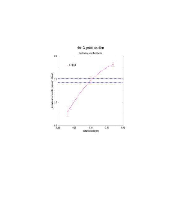
FIG. 26.: The size of the pion, determined from the inverse monopole mass in the pion electromagnetic form, as a function of the instanton size in the random instanton ensemble, from [BS_96]. The horizontal lines show the experimental uncertainty.

Let us now focus on another three-point function which is more directly related to experiment. The pion electromagnetic form factor is determined by the following correlation function

$$\Gamma_{\mu}(x,y) = \langle j^{+}_{5}(-x/2)j^{3}_{\mu}(y)j^{-}_{5}(x/2)\rangle,$$ (319)

where $j_{5}^{\pm}$ are the pseudo-scalar currents of the charged pion and $j^{3}_{\mu}$ is the third component of the isovector-vector current. In this case, the correlator is completely determined by the triangle diagram. In the context of QCD sum rules, the pion form factor is usually analyzed using a three-point functions build from axial-vector currents (because the pseudo-scalar sum rule is known to be unreliable). In the single-instanton approximation the problem was recently studied in [FN_95], where it was shown that including direct instantons (as in Sec. VI C 2), the pion form factor can also be extracted from the pseud-scalar correlator (319). Using the standard instanton liquid parameters, these authors calculated the pion form factor for $Q^{2}\sim 1GeV$, obtaining good agreement with experimental data.

Recently, the three-point function (319) in the instanton liquid was also calculated numerically [BS_96]. In this case, one can go to arbitrarily large distance and determine the pion form factor at small momentum. In this regime, the pion form factor has a simple monopole shape $F_{\pi}(Q^{2})=M^{2}/(Q^{2}+M^{2})$ with a characteristic mass close to the rho meson mass. However, at intermediate momenta $Q^{2}\sim 1$ the pion form factor is less sensitive to the meson cloud and largely determined by the quark-anti-quark interaction inside the pion. In the instanton model, the interaction is dominated by single-instanton effects and the range is controlled by the instanton size. This can be seen from Fig. 26 where we show the fitted monopole mass as a function of the instanton size. Clearly, the two are strongly correlated and the instanton model reproduces the experimental value of the monopole mass if the mean instanton size is $\rho\simeq 0.35$ fm.

Finally, let us mention a few experimental observables that might be interesting in connection with instanton effects in hadronic structure. These are observables that are sensitive to the essential features of the ’t Hooft interaction, the strong correlation between quark and gluon polarization and flavor mixing. The first is the flavor singlet axial coupling constant of the nucleon $g_{A}^{0}$, which is a measure of the quark contribution to the nucleon spin. This quantity can be determined in polarized deep inelastic scattering and was found to be unexpectedly small, $g_{A}^{0}\simeq 0.35$. The quark model suggests $g_{A}^{0}\simeq 1$, a discrepancy which is known as the “proton spin crisis”.

Since $g_{A}^{0}$ is defined by a matrix element of the flavor singlet current, one might suspect that the problem is somehow related to the anomaly. In fact, if it were not for the anomaly, one could not transfer polarization from quarks to gluons and $g_{A}^{0}$ could not evolve. All this suggests that instantons might be crucial in understanding the proton spin structure. While some attempts in this direction have been made [FS_91, DKZ_93], a realistic calculation is still missing.

Another question concerns the flavor structure of the unpolarized quark sea in the nucleon. From measurements of the Gottfried sum rule, the quark sea is known to be flavor asymmetric; there are more $d$ than $u$ quarks in the proton sea. From a perturbative point of view this is puzzling, because gluons are flavor-blind, so a radiatively generated sea is flavor symmetric. However, as pointed out by [DK_93], quark pairs produced by instantons are flavor asymmetric. For example, a valence $u$ quark generates $\bar{d}d,\bar{s}s$ sea, but no $\bar{u}u$ pairs. Since a proton has two valence $u$ quarks, this gives the right sign of the observed asymmetry.

VII Instantons at finite temperature

A Introduction

1 Finite temperature field theory and the caloron solution

In the previous sections we have shown that the instanton liquid model provides a mechanism for chiral symmetry breaking and describes a large number of hadronic correlation functions. Clearly, it is of interest to generalize the model to finite temperature and/or density. This will allow us to study the behavior of hadrons in matter, the mechanism of the chiral phase transition and possible non-perturbative effects in the high temperature/density phase. Extending the methods described in the last three sections to non-zero temperature is fairly straightforward. In euclidean space, finite temperature corresponds to periodic boundary conditions on the fields. Basically, all we have to do is replace all the gauge potentials and fermionic wave functions by their $T\neq 0$ periodic counterparts. Nevertheless, doing so leads to a number of interesting and very non-trivial phenomena, which we will describe in detail below. Extending the instanton model to finite density is more difficult. In Euclidean space a finite chemical potential corresponds to a complex weight in the functional integral, so applying standard methods from statistical mechanics is less straightforward. While some work on the subject has been done [Car_80, Bal_81, Che_81, Shu_82c, Abr_83], many questions remain to be understood.

Before we study the instanton liquid at $T\neq 0$, we would like to give a very brief introduction to finite temperature field theory in Euclidean space [Shu_80, GPY_81, McL_86, Kap_89]. The basic object is the partition function

$$Z = {\rm Tr}(e^{-\beta H}),$$ (320)

where $\beta=1/T$ is the inverse temperature, $H$ is the Hamiltonian and the trace is performed over all physical states. In Euclidean space, the partition function can be written as a functional integral

$$Z = \int_{per}DA_{\mu}\int_{aper}D\bar{\psi}D\psi\,\exp\left(-\int_{0}^{\beta}d\tau\int d^{3}x\,{\cal L}\right),$$ (321)

where the gauge fields and fermions are subject to periodic/anti-periodic boundary conditions

$$A_{\mu}(\vec{r},\beta) = \;\;A_{\mu}(\vec{r},0),$$ (322)

$$\psi(\vec{r},\beta) = -\psi(\vec{r},0),\hskip 14.22636pt\bar{\psi}(\vec{r},\beta)\,=\,-\bar{\psi}(\vec{r},0).$$ (323)

The boundary conditions imply that the fields can be expanded in a Fourier series $\phi(\vec{r},\tau)=e^{i\omega_{n}\tau}\phi_{n}(\vec{r})$, where $\omega_{n}=2\pi nT$ and $\omega_{n}=(2n+1)\pi T$ are the Matsubara frequencies for boson and fermions.

As an example, it is instructive to consider the free propagator of a massless fermion at finite temperature. Summing over all Matsubara frequencies we get

$$S_{T}(r,\tau) = \frac{i}{4\pi^{2}}\gamma\cdot\partial\sum_{n}\frac{(-1)^{n}}{r^{2}+(\tau-n\beta)^{2}}.$$ (324)

The sum can easily be performed, and in the spatial direction one finds

$$S_{T}(r,0) = \frac{i\vec{\gamma}\cdot\vec{r}}{2\pi^{2}r^{4}}z\exp(-z)\frac{(z+1)+(z-1)\exp(-2z)}{(1+\exp(-2z))^{2}},$$ (325)

where $z=\pi rT$. This result shows that at finite temperature, the propagation of massless fermion in the spatial direction is exponentially suppressed. The screening mass $m=\pi T$ is the lowest Matsubara frequency for fermions at finite temperature. The energy $\pi T$ acts like a (chiral) mass term for space-like propagation. For bosons, on the other hand, the wave functions are periodic, the lowest Matsubara frequency is zero and the propagator is not screened. The propagator in the temporal direction is given by

$$S_{T}(0,\tau) = \frac{i\gamma_{4}}{2\pi^{2}\tau^{3}}\frac{y^{3}}{2}\frac{1+\cos^{2}(y)}{\sin^{3}(y)},$$ (326)

with $y=\pi\tau T$. Clearly, there is no suppression factor for propagation in the temporal direction.

Periodic instanton configurations can be constructed by lining up zero temperature instantons along the imaginary time direction with the period $\beta$. Using ’t Hoofts multi-instanton solution (A7), the explicit expression for the gauge field is given by [HS_78]

$$A_{\mu}^{a} = \overline{\eta}^{a}_{\mu\nu}\Pi(x)\partial_{\nu}\Pi^{-1}(x)$$ (327)

where

$$\Pi(x) = 1+\frac{\pi\rho^{2}}{\beta r}\frac{\sinh(2\pi r/\beta)}{\cosh(2\pi r/\beta)-\cos(2\pi\tau/\beta)}$$ (328)

Here, $\rho$ denotes the size of the instanton. The solution (327) is sometimes referred to as the caloron. It has topological charge $Q=1$ and action $S=8\pi^{2}/g^{2}$ independent of temperature. A caloron with $Q=-1$ can be constructed making the replacement $\overline{\eta}^{a}_{\mu\nu}\to\eta^{a}_{\mu\nu}$. Of course, as $T\to 0$ the caloron field reduces to the field of an instanton. In the high temperature limit $T\rho\gg 1$, however, the field looks very different [GPY_81]. In this case, the caloron develops a core of size $O(\beta)$ where the fields are very strong $G_{\mu\nu}\sim O(\beta^{2})$. In the intermediate regime $O(\beta)<r<O(\rho^{2}/\beta)$ the caloron looks like a ($T$ independent) dyon with unit electric and magnetic charges,

$$E_{i}^{a}=B_{i}^{a}\simeq\frac{\hat{r}^{a}\hat{r}^{i}}{r^{2}}.$$ (329)

In the far region, $r>O(\rho^{2}/\beta)$, the caloron resembles a three dimensional dipole field, $E_{i}^{a}=B_{i}^{a}\sim O(1/r^{3})$.

At finite temperature, tunneling between degenerate classical vacua is related to the anomaly in exactly the same way as it is at $T=0$. This means that during tunneling, the fermion vacuum is rearranged and that the Dirac operator in the caloron field has a normalizable left handed zero mode. This zero mode can be constructed from the zero modes of the exact $n$-instanton solution [Gro_77]. The result is

$$\psi_{i}^{a} = \frac{1}{2\sqrt{2}\pi\rho}\sqrt{\Pi(x)}\partial_{\mu}\left(\frac{\Phi(x)}{\Pi(x)}\right)\left(\frac{1-\gamma_{5}}{2}\gamma_{\mu}\right)_{ij}\epsilon_{aj}\,,$$ (330)

where $\Phi(x)=(\Pi(x)-1)\cos(\pi\tau/\beta)/\cosh(\pi r/\beta)$. Note that the zero-mode wave function also shows an exponential decay $\exp(-\pi rT)$ in the spatial direction, despite the fact the eigenvalue of the Dirac operator is exactly zero. This will have important consequences for instanton interactions at non-zero temperature.

2 Instantons at high temperature

At finite temperature, just like at $T=0$, the instanton density is controlled by fluctuations around the classical caloron solution. In the high temperature plasma phase, the gluoelectric fields in the caloron are Debye screened, so we expect that instantons are strongly suppressed at high temperature [Shu_78]. The perturbative Debye mass in the quark-gluon plasma is [Shu_78b]

$$m_{D}^{2}=(N_{c}/3+N_{f}/6)g^{2}T^{2}.$$ (331)

Normal $O(1)$ electric fields are screened at distances $1/(gT)$, while the stronger $O(1/g)$ non-perturbative fields of the instantons should be screened for sizes $\rho>T^{-1}$. An explicit calculation of the quantum fluctuations around the caloron was performed by Pisarski and Yaffe [PY_80]. Their result is

$$n(\rho,T) = n(\rho,T=0)\exp\left(-\frac{1}{3}(2N_{c}+N_{f})(\pi\rho T)^{2}-B(\lambda)\right)$$ (332)

$$B(\lambda) = \left(1+\frac{N_{c}}{6}-\frac{N_{f}}{6}\right)\left(-\log\left(1+\frac{\lambda^{2}}{3}\right)+\frac{0.15}{(1+0.15\lambda^{-3/2})^{8}}\right)$$ (333)

where $\lambda=\pi\rho T$. As expected, large instantons $\rho\gg 1/T$ are exponentially suppressed. This means that the instanton contribution to physical quantities like the energy density (or pressure, etc.) is of the order

$$\epsilon(T)\sim\int^{1/T}_{0}{d\rho\over\rho^{5}}(\rho\Lambda)^{b}\sim T^{4}(\Lambda/T)^{b}.$$ (334)

At high temperature, this is small compared to the energy density of an ideal gas $\epsilon(T)_{SB}\sim T^{4}$.

It was emphasized in [SV_94] that although the Pisarski-Yaffe result contains only one dimensionless parameter $\lambda$, its applicability is controlled by two separate conditions:

$$\rho\ll 1/\Lambda,\hskip 28.45274ptT\gg\Lambda.$$ (335)

The first condition ensures the validity of the semi-classical approximation, while the second justifies the perturbative treatment of the heat bath. In order to illustrate this point, we would like to discuss the derivation of the semi-classical result (332) in somewhat more detail. Our first point is that the finite temperature correction to the instanton density can be split into two parts of different physical origin. For this purpose, let us consider the determinant of a scalar field in the fundamental representation. The temperature dependent part of the one loop effective action

$$\left.\log\det\left(\frac{-D^{2}}{-\partial^{2}}\right)\right|_{T} = \left.\log\det\left(\frac{-D^{2}}{-\partial^{2}}\right)\right|_{T=0}+\delta$$ (336)

can be split into two pieces, $\delta=\delta_{1}+\delta_{2}$, where

$$\delta_{1} = {\rm Tr}_{T}\log\left(\frac{-D^{2}(A(\rho))}{-\partial^{2}}\right)-{\rm Tr}\log\left(\frac{-D^{2}(A(\rho))}{-\partial^{2}}\right),$$ (337)

$$\delta_{2} = {\rm Tr}_{T}\log\left(\frac{-D^{2}(A(\rho,T))}{-\partial^{2}}\right)-{\rm Tr}_{T}\log\left(\frac{-D^{2}(A(\rho))}{-\partial^{2}}\right).$$ (338)

Here $Tr_{T}$ includes an integration over $R^{3}\times[0,\beta]$, and $A(\rho,T)$, $A(\rho)$ are the gauge potentials of the caloron and the instanton, respectively. The two terms $\delta_{1}$ and $\delta_{2}$ correspond to the two terms in the exponent in the semi-classical result (332).

It was shown in [Shu_82c] that the physical origin of the first term is scattering of particles in the heath bath on the instanton field. The forward scattering amplitude $T(p,p)$ of a scalar quark can be calculated using the standard LSZ reduction formula

$${\rm Tr}\left(T(p,p)\right) = \int d^{4}xd^{4}y\ e^{ip\cdot(x-y)}{\rm Tr}\left(\partial^{2}_{x}\Delta(x,y)\partial^{2}_{y}\right)$$ (339)

where $\Delta(x,y)$ is the scalar quark propagator introduced in Sec. VI B 1. By subtracting the trace of the free propagator and going to the physical pole $p^{2}=0$ one gets a very simple answer

$${\rm Tr}\left(T(p,p)\right) = \,-4\pi^{2}\rho^{2}.$$ (340)

Since the result is just a constant, there is no problem with analytic continuation to Minkowski space. Integrating the result over a thermal distribution, we get

$$\delta_{1} = \int{d^{3}p\over(2\pi)^{3}}{1\over 2p(\exp(p/T)-1)}{\rm Tr}\left(T(p,p)\right)\,=\,-\frac{1}{6}(\pi\rho T)^{2}\,=\,-\frac{1}{6}\lambda^{2}$$ (341)

The constant appearing in the result are easily interpreted: $\rho^{2}$ comes from the scattering amplitude, while the temperature dependence enters via the integral over the heat bath. Also note that the scattering amplitude has the same origin (and the same dependence on $N_{c},N_{f}$) as the Debye mass.

Formally, the validity of this perturbative calculation requires that $g(T)\ll 1$, but in QCD this criterion is satisfied only at extremely high temperature. We would argue, however, that the accuracy of the calculation is controlled by the same effects that determine the validity of the perturbative result for the Debye mass. Available lattice data [Irb_91] suggest that screening sets in right after the phase transition, and that the perturbative prediction for the Debye mass works to about 10% accuracy for $T>3T_{c}\simeq 500$ MeV. Near the critical temperature one expects that the Debye mass becomes small; screening disappears together with the plasma. Below $T_{c}$ the instanton density should be determined by the scattering of hadrons, not quarks and gluons, on the instanton. We will return to this point in the next section.

The second term in the finite temperature effective action (338) has a different physical origin. It is determined by quantum corrections to the colored current [BC_78], multiplied by the $T$-dependent variation of the instanton field, the difference between the caloron and the instanton. For $\lambda$ small, the correction is given by

$$\delta_{2}=-\frac{1}{36}\lambda^{2}+O(\lambda^{3}).$$ (342)

The result has the same sign and the same dependence on the parameters as $\delta_{1}$, but a smaller coefficient. Thus, finite $T$ effects not only lead to the appearance of the usual (perturbative) heat bath, they also modify the strong $O(1/g)$ classical gauge field of the instanton. In Euclidean space, we can think of this effect as arising from the interaction of the instanton with its periodic “mirror images” along the imaginary time direction. However, below $T_{c}$, gluon correlators are exponentially suppressed since glueballs states are very heavy. Therefore, we expect that for $T<T_{c}$, the instanton field is not modified by the boundary conditions. Up to effects of the order $O(\exp(-M/T))$, where $M$ is the mass of the lowest glueball, there is no instanton suppression due to the change in the classical field below $T_{c}$.

3 Instantons at low temperature

The behavior of the instanton density at low temperature was studied in [SV_94]. At temperatures well below the phase transition the heat bath consists of weakly interacting pions. The interaction of the pions in the heat bath with instantons can be determined from the effective Lagrangian (120). For two flavors, this Lagrangian is a product of certain four-fermion operators and the semi-classical single instanton density. In the last section, we argued that the semi-classical instanton density is not modified at small temperature. The temperature dependence is then determined by the $T$ dependence of the vacuum expectation value of the four-fermion operators. For small $T$, the situation can be simplified even further, because the wavelength of the pions in the heat bath is large and the four-fermion operators can be considered local.

The temperature dependence of the expectation value of a general four-fermion operator $\langle(\bar{q}Aq)(\bar{q}Bq)\rangle$ can be determined using soft pion techniques [GL_89]. To order $T^{2}/f_{\pi}^{2}$ the result is determined by the matrix element of the operator between one-pion states, integrated over a thermal pion distribution. The one-pion matrix element can be calculated using the reduction formula and current algebra commutators. These methods allow us to prove the general formula [Ele_93]

$$\langle(\bar{q}Aq)(\bar{q}Bq)\rangle_{T} = \langle(\bar{q}Aq)(\bar{q}Bq)\rangle_{0}-{T^{2}\over 96f^{2}_{\pi}}\langle(\bar{q}\{\Gamma^{a}_{5},\{\Gamma_{5}^{a},A\}\}q)(\bar{q}Bq)\rangle_{0}$$ (344)

$$-{T^{2}\over 96f^{2}_{\pi}}\langle(\bar{q}Aq)(\bar{q}\{\Gamma^{a}_{5},\{\Gamma^{a}_{5},B\}\}q)\rangle_{0}-{T^{2}\over 48f^{2}_{\pi}}\langle(\bar{q}\{\Gamma^{a}_{5},A\}q)(\bar{q}\{\Gamma^{a}_{5},B\}q)\rangle_{0},$$

where $A,B$ are arbitrary flavor-spin-color matrices and $\Gamma_{5}^{a}=\tau^{a}\gamma_{5}$. Using this result, the instanton density at low temperature is given by

$$n(\rho,T) = n(\rho)\left(\frac{4}{3}\pi^{2}\rho^{3}\right)^{2}\left[\langle K_{1}\rangle_{0}\frac{1}{4}\left(1-\frac{T^{2}}{6f^{2}_{\pi}}\right)-\langle K_{2}\rangle_{0}\frac{1}{12}\left(1+\frac{T^{2}}{6f^{2}_{\pi}}\right)\right],$$ (345)

where we have defined the two operators ($\tau$ are isospin matrices):

$$K_{1} = \bar{q}_{L}q_{L}\bar{q}_{L}q_{L}+{3\over 32}\bar{q}_{L}\lambda^{a}q_{L}\bar{q}_{L}\lambda^{a}q_{L}-{9\over 128}\bar{q}_{L}\sigma_{\mu\nu}\lambda^{a}q_{L}\bar{q}_{L}\sigma_{\mu\nu}\lambda^{a}q_{L},$$ (346)

$$K_{2} = \bar{q}_{L}\tau^{i}q_{L}\bar{q}_{L}\tau^{i}q_{L}+{3\over 32}\bar{q}_{L}\tau^{i}\lambda^{a}q_{L}\bar{q}_{L}\tau^{i}\lambda^{a}q_{L}-{9\over 128}\bar{q}_{L}\sigma_{\mu\nu}\tau^{i}\lambda^{a}q_{L}\bar{q}_{L}\sigma_{\mu\nu}\tau^{i}\lambda^{a}q_{L}.$$ (347)

Although the vacuum expectation values of these two operators are unknown, it is clear that (baring unexpected cancellations) the $T$ dependence should be rather weak, most likely inside the range $n=n_{0}(1\pm T^{2}/(6f^{2}_{\pi}))$. Furthermore, if one estimates the expectation values using the factorization assumption (181), the $T$ dependence cancels to order $T^{2}/f_{\pi}^{2}$.

Summarizing the last two sections we conclude that the instanton density is expected to be essentially constant below the phase transition, but exponentially suppressed at large temperature. We will explore the physical consequences of this result in the remainder of this chapter. Numerical evidence for our conclusions that comes from lattice simulations will be presented in Sec. VII D.

4 Instanton interaction at finite temperature

FIG. 27.: Instanton-anti-instanton interaction at finite temperature. Fig.a) shows the pure gauge interaction in units of $S_{0}$ as a function of the spatial separation in units of $\rho$. The temperature is given in MeV for $\rho=0.33$ fm. Fig. b) shows the fermionic overlap matrix element $T_{IA}$ for spatial separation $r$ and Fig. c) for temporal separation $\tau$.

In order to study an interacting system of instantons at finite temperature, we need to determine the bosonic and fermionic interaction between instantons at $T\neq 0$. This subject was studied in [DM_88] and later, in much greater detail, in [SV_91], which we will follow here. As for $T=0$, the gluonic interactions between an instantons and an anti-instanton is defined as $S_{int}=S[A_{IA}]-2S_{0}$, where we have to specify an ansatz $A_{IA}$ for the gauge potential of the $IA$ configuration. The main difficulty at $T\neq 0$ is that Lorenz invariance is lost and the interaction depends on more variables: the spatial and temporal separation $r,\tau$ of the instantons, the sizes $\rho_{I},\rho_{A}$, the relative orientation matrix $U$ and the temperature $T$. Also, there are more invariant structures that can be constructed from the relative orientation vector $u_{\mu}$. In the case of color $SU(2)$, we have

$$S_{IA} = s_{0}+s_{1}(u\cdot\hat{R})^{2}+s_{2}(u\cdot\hat{R})^{4}+s_{3}(u^{2}-(u\cdot\hat{R})^{2}-u_{4}^{2})$$ (349)

$$+s_{4}(u^{2}-(u\cdot\hat{R})^{2}-u_{4}^{2})^{2}+s_{5}(u\cdot\hat{R})^{2}(u^{2}-(u\cdot\hat{R})^{2}-u_{4}^{2}),$$

where $s_{i}=s_{i}(r,\tau,\rho_{I},\rho_{A},\beta)$. Because of the reduced symmetry of the problem, it is difficult to implement the streamline method. Instead, we will study the interaction in the ratio ansatz. The gauge field potential is given by a straightforward generalization of (151). Except for certain limits, the interaction cannot be obtained analytically. We therefore give a parameterization of the numerical results obtained in [SV_91]

$$S_{IA} = \frac{8\pi^{2}}{g^{2}}\bigg{\{}\frac{4.0}{(r^{2}+2.0)^{2}}\frac{\beta^{2}}{\beta^{2}+5.21}|u|^{2}-\left[\frac{1.66}{(1+1.68r^{2})^{3}}+\frac{0.72\log(r^{2})}{(1+0.42r^{2})^{4}}\right]\frac{\beta^{2}}{\beta^{2}+0.75}|u|^{2}$$ (352)

$$\hskip 17.07182pt+\left[-\frac{16.0}{(r^{2}+2.0)^{2}}+\frac{2.73}{(1+0.33r^{2})^{3}}\right]\frac{\beta^{2}}{\beta^{2}+0.24+11.50r^{2}/(1+1.14r^{2})}|u\cdot\hat{R}|^{2}$$

$$\hskip 17.07182pt+0.36\log\left(1+\frac{\beta}{r}\right)\frac{1}{(1+0.013r^{2})^{4}}\frac{1}{\beta^{2}+1.73}(|u|^{2}-|u\cdot\hat{R}|^{2}-|u_{4}|^{2})\bigg{\}}$$

This parameterization is shown in Fig. 27. We observe that the qualitative form of the interaction does not change, but it becomes more short range as the temperature increases. This is a consequence of the core in the instanton gauge field discussed above. At temperatures $T<1/(3\rho)$ the interaction is essentially isotropic. As we will see below, this is not the case for the fermionic matrix elements.

The fermion determinant is calculated from the overlap matrix elements $T_{IA}$ with the finite temperature zero mode wave functions. Again, the orientational dependence is more complicated at $T\neq 0$. We have

$$T_{IA} = u_{4}f_{1}+\vec{u}\cdot\hat{r}f_{2}$$ (353)

where $f_{i}=f_{i}(r,\tau,\rho_{I},\rho_{A},\beta)$. The asymptotic form of $T_{IA}$ for large temperatures $\beta\to 0,R\to\infty$ can be determined analytically. The result is [SV_91, KY_91]

$$f_{1}^{as} = i\frac{\pi^{2}}{\beta}\sin\left(\frac{\pi\tau}{\beta}\right)\exp\left(-\frac{\pi r}{\beta}\right),$$ (354)

$$f_{2}^{as} = i\frac{\pi^{2}}{\beta}\cos\left(\frac{\pi\tau}{\beta}\right)\exp\left(-\frac{\pi r}{\beta}\right).$$ (355)

A parameterization of the full result is shown in Fig. 27 [SS_96b]. The essential features of the result can be seen from the asymptotic form (354,355): At large temperature, $T_{IA}$ is very anisotropic. The matrix element is exponentially suppressed in the spatial direction and periodic along the temporal axis. The exponential decay in spatial direction is governed by the lowest Matsubara frequency $\pi T$. The qualitative behavior of $T_{IA}$ has important consequences for the structure of the instanton liquid at $T\neq 0$. In particular, the overlap matrix element favors the formation of instanton-anti-instanton molecules oriented along the time direction.

FIG. 28.: (a) Fermionic overlap matrix element $T_{IA}(\tau,r=0,T=T_{c})$ as a function of the distance $\tau$ between the centers of the instanton and anti-instanton in the time direction. (b) Same for the partially integrated partition function $Z_{mol}^{\prime}=\int d^{10}\Omega T^{2N_{f}}_{IA}e^{-S_{int}}$, ($Z$ is not yet integrated over Matsubara time) at different temperatures $T=(0.6-1.0)T_{c}$ (in steps of $\Delta T=0.04T_{c}$). The dashed line shows the behaviour of $T_{IA}$. (c,d) Fermionic overlap matrix element and partition function after integration over Matsubara time.

These configurations were studied in more detail in [SV_96]. These authors calculate the IA partition function (163) from the bosonic and fermionic interaction at finite temperature. The integration over the collective coordinates was performed as follows: The point $r=0$ (same position in space) and the most attractive relative orientation ($U=1,\,\cos\theta=1$) are maxima of the partition function, so one can directly use the saddle point method for 10 integrals out of 11 (3 over relative spatial distance between the centers and over 7 relative orientation angles). The remaining integral over the temporal distance $\tau$ is more complicated and has to be done numerically.

In Fig. 28(a) we show the dependence of the overlap matrix element $T_{IA}$ on $\tau$ for $T=T_{c}$, $r=0$ and $U=1$. Even at $T_{c}$, $T_{IA}$ does not have a maximum at the symmetric point $\tau=1/(2T)$, but a minimum. However, when one includes the bosonic interaction and the pre-exponential factor from taking into account fluctuations around the saddle-point, the result looks different. The partition function after integrating over 10 of the 11 collective coordinates is shown in Fig. 28(b) for temperatures in the range $(0.6-1.0)T_{c}$. We observe that there is a maximum in the partition function at the symmetric point $\tau=1/(2T)$ if the temperature is bigger than $T_{molec}\simeq 0.2\rho\simeq 120$ MeV. The temperature dependence of the partition function integrated over all variables is shown in Fig. 28(c,d).

This means that there is a qualitative difference between the status of instanton-anti-instanton molecules at low and high ($T>T_{molec}$) temperature. At low temperature, saddle points in the instanton-anti-instanton separation only exist if the collective coordinates are analytically continued into the complex plane (as in Sec. II A). At high temperature there is a real saddle point in the middle of the Matsubara box ($\tau=1/(2T)$), which gives a real contribution to the free energy. It is important that this happens close to the chiral phase transition. In fact, we will argue that the phase transition is caused by the formation of these molecules.

B Chiral symmetry restoration

1 Introduction to QCD phase transitions

Before we come to a detailed discussion of the instanton liquid at finite temperature, we would like to give a brief summary of what is known about the phase structure of QCD at finite temperature. It is generally believed that at high temperature (or density) QCD undergoes a phase transition from hadronic matter to the quark-gluon plasma (QGP). In the plasma phase color charges are screened [Shu_78b] rather then confined, and chiral symmetry is restored. At sufficiently high temperature perturbation theory should be applicable and the physical excitations are quarks and gluons. In this case, the thermodynamics of the plasma is governed by the Stefan-Boltzmann law, just like ordinary black body radiation.

FIG. 29.: Equation of state for $N_{f}=2$ QCD with Kogut-Susskind fermions, from [BKT_95].

This basic scenario has been confirmed by a large number of lattice simulations. As an example, we show the equation of state for $N_{f}=2$ (Kogut-Susskind) QCD in Fig. 29 [BKT_95]. The transition temperature is $T_{c}(N_{f}=2)\simeq 150$ MeV. The energy density and pressure are small below the phase transition, but the energy density rises quickly to its perturbative (Stefan Boltzmann) value. The pressure, on the other hand, lags behind and remains small up to $T\simeq 2T_{c}$.

In Fig. 29 the energy density and pressure are measured with respect to the perturbative vacuum. However, we have repeatedly emphasized that in QCD, there is a non-perturbative vacuum energy density (the bag pressure) even at $T=0$. In order to compare a non-interacting gas of quarks and gluons with the hadronic phase, we have to shift the pressure in the high $T$ phase by this amount, $p_{QGP}\to p_{QGP}-B$. Since the pressure from thermal hadrons below $T_{c}$ is small, a rough estimate of the transition temperature can be obtained from the requirement that the (shifted) pressure in the plasma phase is positive, $p_{QGP}>0$. From this inequality we expect the plasma phase to be favored for $T>T_{c}=[(90B)/(N_{d}\pi^{2})]^{1/4}$, where $N_{d}$ is the effective number of degrees of freedom in the QGP phase. For $N_{f}=2$ we have $N_{d}=37$ and $T_{c}\simeq 180$ MeV.

Lattice simulations indicate that in going from quenched QCD to QCD with two light flavors the transition temperature drops by almost a factor of two, from $T_{c}(N_{f}=0)\simeq 260$ MeV to $T_{c}(N_{f}=2)\simeq 150$ MeV. The number of degrees of freedom in the plasma phase, on the other hand, increases only from 16 to 37 (and $T_{c}$ does not vary very much with $N_{d}$, $T_{c}\sim N_{d}^{-1/4}$). This implies that there are significant differences between the pure gauge and unquenched phase transitions.

In particular, the low transition temperature observed for $N_{f}=2,3$ suggests that the energy scales are quite different. We have already emphasized that the bag pressure is directly related to the gluon condensate [Shu_78]. This relation was studied in more detail in [AHZ_91, Den_89, KB_93]. From the canonical energy momentum tensor and the trace anomaly, the gluonic contributions to the energy density and pressure are related to the electric and magnetic field strengths

$$\epsilon = {1\over 2}\langle B^{2}-E^{2}\rangle-{g^{2}b\over 128\pi^{2}}\langle E^{2}+B^{2}\rangle,$$ (356)

$$p = {1\over 6}\langle B^{2}-E^{2}\rangle+{g^{2}b\over 128\pi^{2}}\langle E^{2}+B^{2}\rangle.$$ (357)

Using the available lattice data one finds that in pure gauge theory the gluon condensate essentially disappears in the high temperature phase, while in full QCD ($N_{f}=2,3$) about half of the condensate remains. G. Brown has referred to this part of the gluon condensate as the “hard glue” or “epoxy”. It plays an important role in keeping the pressure positive despite the low transition temperature.

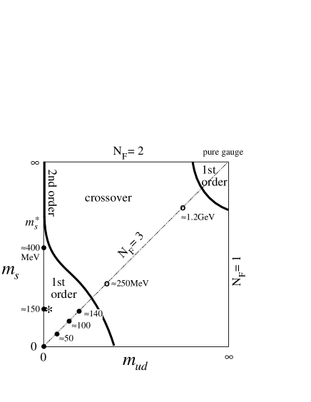
FIG. 30.: Schematic phase diagram of $N_{f}=3$ QCD with dynamical quark masses $m_{ud}\equiv m_{u}=m_{d}$ and $m_{s}$, from [IKK_96]. Solid and open points mark simulations (with Wilson fermions) that found a first order transition or a smooth crossover, respectively. The (approximate) location of QCD with realistic masses is shown by a star.

More general information on the nature of the phase transition is provided by universality arguments. For this purpose, we have to identify an order parameter that characterizes the transition. In QCD, there are two limits in which this can be achieved. For infinitely heavy quarks, the Polyakov line [Pol_78] provides an order parameter for the deconfinement transition, while for massless quarks the fermion condensate is an order parameter for spontaneous chiral symmetry breaking. The Polyakov line is defined by

$$\langle L(\vec{x})\rangle = \langle P\exp\left(i\int_{0}^{\beta}d\tau\,A_{0}(\vec{x},\tau)\right)\rangle,$$ (358)

which can be interpreted as the propagator of a heavy quark. The free energy of a single static quark (minus the free energy of the vacuum) is given by $F_{q}-F_{0}=-T\log(|\langle L(\vec{x})\rangle|)$. For $\langle L\rangle=0$, the free energy of an isolated quark is infinite and the theory is in the confining phase. For $\langle L\rangle\neq 0$ the free energy is finite, and quarks are screened rather than confined.

The Polyakov line has a nontrivial symmetry. Under gauge transformations in the center of the gauge group $Z_{N_{c}}\subset SU(N_{c})$ local observables are invariant but the Polyakov line picks up a phase $L\to zL$ with $z\in Z_{N_{c}}$. The deconfinement transition was therefore related with spontaneous breakdown of the $Z_{N_{c}}$ center symmetry. Following Landau, long wave excitations near the phase transition should be governed by an effective $Z_{N_{c}}$ symmetric Lagrangian for the Polyakov line [SY_82]. Since long range properties are determined by the lowest Matsubara modes, the effective action is defined in three dimensions. For $N_{c}=2$, this means that the transition is in the same universality class as the $d=3$ Ising model, which is known to have a second order phase transition. For $N_{c}\geq 3$, on the other hand, we expect the transition to be first order. These expectations are supported by lattice results.

For massless quarks chiral symmetry is exact, and the quark condensate $\langle\bar{q}q\rangle$ provides a natural order parameter. The symmetry of the order parameter is determined by the transformation properties of the matrix $U_{ij}=\langle\bar{q}_{i}q_{j}\rangle$. For $N_{f}=2$ flavors, this symmetry is given by $SU(2)\times SU(2)=O(4)$, so the transition is governed by the effective Lagrangian for a four dimensional vector field in three dimension [PW_84, Wil_92, RW_93]. The $O(4)$ Heisenberg magnet is known to have a second order phase transition and the critical indices have been determined from both numerical simulations and the $\epsilon$ expansion. For $N_{f}\geq 3$, however, the phase transition is predicted to be first order.

From these arguments, one expects the schematic phase structure of QCD in the $m_{ud}-m_{s}$ (with $m_{ud}\equiv m_{u}=m_{d}$) plane to look as shown in Fig. 30 [BBC_90, IKK_96]. The upper right hand corner corresponds to the first order purge gauge phase transition. Presumably, this first order transition extends to lower quark masses, before it ends in a line of second order phase transitions. The first order $N_{f}=3$ chiral phase transition is located in the lower left corner, and continues in the mass plane before it ends in another line of second order phase transitions. At the left edge there is a tri-critical point where this line meets the line of $N_{f}=2$ second order phase transitions extending down from the upper left corner.

Simulations suggest that the gap between the first order chiral and deconfinement transitions is very wide, extending from $m\equiv m_{u}=m_{d}=m_{s}\simeq 0.2$ GeV to $m\simeq 0.8$ GeV. This is in line with the arguments given above, indicating that there are important differences between the phase transitions in pure gauge and full QCD. Nevertheless, one should not take this distinction to literally. In the presence of light quarks, there is no deconfinement phase transition in a strict, mathematical, sense. From a practical point of view, however, deconfinement plays an important role in the chiral transition. In particular, the equation of state shows that the jump in energy density is dominated by the release of 37 quark and gluon degrees of freedom.

There are many important questions related to the phase diagram that still have to be resolved. First of all, we have to determine the location of real QCD (with two light, one intermediate mass and several heavy flavors) on this phase diagram. While results using staggered fermions [BBC_90] seem to suggest that QCD lies outside the range of first order chiral phase transitions and only shows a smooth crossover, simulations using Wilson fermions [Iwa_91] with realistic masses find a first order transition.

A more general is problem is to verify the structure of the phase diagram and to check the values of the critical indices near second order transitions. While earlier studies confirmed (within errors) the $O(4)$ values of the critical indices for the $N_{f}=2$ chiral transition with both staggered [KL_94] and Wilson fermions [IKK_96], more recent work concludes that $1/\delta$ (defined as $\langle\bar{q}q\rangle_{T_{c}}\sim m^{1/\delta}$) is consistent with zero [Ukawa_96]. If this result is correct, it would imply that there is no $N_{f}=2$ second order phase transition and the only second order line in Fig. 30 corresponds to the boundary of the first order region, with standard Ising indices.

Are there any possible effects that could upset the expected $O(4)$ scenario for the $N_{f}=2$ transition? One possibility discussed in the literature is related to the fate of the $U(1)_{A}$ symmetry at $T_{c}$. At zero temperature the axial $U(1)_{A}$ symmetry is explicitly broken by the chiral anomaly and instantons. If instantons are strongly suppressed [PW_84] or rearranged [Shu_94] at $T_{c}$, then the $U(1)_{A}$ symmetry might effectively be restored at the phase transition. In this case, the masses of the $U(1)_{A}$ partners of the $\pi,\sigma$, the $\delta,\eta^{\prime}$, could become sufficiently small so that fluctuations of these modes affect the universality arguments given above. In particular, if there are eight rather than four light modes at the phase transition, the transition is expected to be first order. Whether this is the correct interpretation of the lattice data remains unclear at the moment. We will return to the question of $U(1)_{A}$ breaking at finite temperature in Sec. VII C 3 below. Let us only note that the simulations are very difficult and that there are several possible artefacts. For example, there could be problems with the extrapolation to small masses. Also, first order transitions need not have an order parameter, and it is difficult to distinguish very weak first order transitions from second order transitions.

Completing this brief review of general arguments and lattice results on the chiral phase transition, let us also comment on some of the theoretical approaches. Just like perturbative QCD describes the thermodynamics of the plasma phase at very high temperature, effective chiral lagrangian provide a very powerful tool at low temperature. In particular, chiral perturbation theory predicts the temperature dependence of the quark and gluon condensates as well as of the masses and coupling constants of light hadrons [GL_89]. These results are expressed as an expansion in $T^{2}/f_{\pi}^{2}$. It is difficult to determine what the range of validity of these predictions is, but the approach certainly has to fail as one approaches the phase transition.

In addition to that, the phase transition has been studied in various effective models, for example in the linear sigma model, the chiral quark model or the Nambu-Jona-Lasinio model [HK_85b, BM_88, KLW_90]. In the NJL model, the chiral transition connects the low temperature phase of massive constituent quarks with the high temperature phase of massless quarks (but of course not gluons). The mechanism for the transition is similar to the transition from a superconductor to a normal metal: The energy gain due to pairing disappears once a sufficient number of positive energy states is excited. We have seen that at zero temperature, the instanton liquid leads to a picture of chiral symmetry breaking which closely resembles the NJL model. Nevertheless, we will argue that the mechanism for the phase transition is quite different. In the instanton liquid, it is the ensemble itself which is rearranged at $T_{c}$. This means that not only do we have non-zero occupation numbers, but the effective interaction itself changes.

Finally, a number of authors have extended random matrix models to finite temperature and density [JV_96, WSW_96, NPZ_96]. It is important to distinguish these models from random matrix methods at $T,\mu=0$. In this case, there is evidence that certain observables, like scaled correlations between eigenvalues of the Dirac operator, are universal and can be described in terms of suitably chosen random matrix ensembles. The effects of non-zero temperature and density, on the other hand, are included in a rather schematic fashion, by putting terms like $(\pi T+i\mu)$ into the Dirac operator. This procedure is certainly not universal. From the point of view of the instanton model, the entries of the random matrix correspond to matrix elements of the Dirac operator in the zero mode basis. If we include the effects of a non-zero $\mu,T$ in the schematic form mentioned above, we assume that at $\mu,T\neq 0$ there are no zero modes in the spectrum. But this is not true, we have explicitly constructed the zero-mode for the caloron configuration in Sec. VII A 1, for $\mu\neq 0$ see [Car_80, Abr_83]. As we will see below, in the instanton model the phase transition is not caused by a constant contribution to the overlap matrix elements, but by specific correlations in the ensemble.

2 The instanton liquid at finite temperature and $IA$ molecules

In Sec. VII A 3, we argued that the instanton density remains roughly constant below the phase transition. This means that the chiral phase transition has to be caused by a rearrangement of the instanton ensemble. Furthermore, we have shown that the gluonic interaction between instantons remains qualitatively unchanged even at fairly high temperatures. This suggests that fermionic interactions between instantons drive the phase transition [IS_94, SSV_95, SS_96].

The mechanism for this transition is most easily understood by considering the fermion determinant for one instanton-anti-instanton pair [SSV_95]. Using the asymptotic form of the overlap matrix elements specified above, we have

$$\det(D\!\!\!\!/\,) \sim \left|\frac{\sin(\pi T\tau)}{\cosh(\pi Tr)}\right|^{2N_{f}}.$$ (359)

This expression is maximal for $r=0$ and $\tau=1/(2T)$, which is the most symmetric orientation of the instanton-anti-instanton pair on the Matsubara torus. Since the fermion determinant controls the probability of the configuration, we expect polarized molecules to become important at finite temperature. The effect should be largest, when the IA pairs exactly fit onto the torus, i.e. $4\rho\simeq\beta$. Using the zero temperature value $\rho\simeq 0.33$ fm, we get $T\simeq 150$ MeV, close to the expected transition temperature for two flavors.

In general, the formation of molecules is controlled by the competition between minimum action, which favors correlations, and maximum entropy, which favors randomness. Determining the exact composition of the instanton liquid as well as the transition temperature requires the calculation of the full partition function, including the fermion induced correlations. We will do this using a schematic model in Sec. VII B 3 and using numerical simulations in Sec. VII B 4.

Before we come to this we would like to study what physical effects are caused by the presence of molecules. Qualitatively, it is clear why the formation of molecules leads to chiral symmetry restoration. If instantons are bound into pairs, then quarks mostly propagate from one instanton to the corresponding anti-instanton and back. In addition to that, quarks propagate mostly along the imaginary time direction, so all eigenstates are well localized in space, and no quark condensate is formed. Another way to see this is by noting that the Dirac operator essentially decomposes into $2\times 2$ blocks corresponding to the instanton-anti-instanton pairs. This means that the eigenvalues will be concentrated around some typical $\pm\lambda$ determined by the average size of the pair, so the density of eigenvalues near $\lambda=0$ vanishes. We have studied the eigenvalue distribution in a schematic model of random and correlated instantons in [SSV_95], and a random matrix model of the transition based on these ideas was discussed in [WSW_96].

The effect of molecules on the effective interaction between quarks at high temperature was studied in [SSV_95], using methods similar to the ones introduced in Sec. IV F. In order to determine the interaction in a quark-anti-quark (meson) channel with given quantum numbers, it is convenient to calculate both the direct and the exchange terms, and Fierz-rearrange the exchange term into an effective direct interaction. The resulting Fierz symmetric Lagrangian reads [SSV_95]

$${\cal L}_{mol\,sym} = G\left\{\frac{2}{N_{c}^{2}}\left[(\bar{\psi}\tau^{a}\psi)^{2}-(\bar{\psi}\tau^{a}\gamma_{5}\psi)^{2}\right]\right.$$ (361)

$$-\;\,\frac{1}{2N_{c}^{2}}\left.\left[(\bar{\psi}\tau^{a}\gamma_{\mu}\psi)^{2}+(\bar{\psi}\tau^{a}\gamma_{\mu}\gamma_{5}\psi)^{2}\right]+\frac{2}{N_{c}^{2}}(\bar{\psi}\gamma_{\mu}\gamma_{5}\psi)^{2}\right\}+{\cal L}_{8},$$

with the coupling constant

$$G = \int n(\rho_{1},\rho_{2})\,d\rho_{1}d\rho_{2}\,\frac{1}{8T_{IA}^{2}}(2\pi\rho_{1})^{2}(2\pi\rho_{2})^{2}\,.$$ (362)

Here, ${\cal L}_{8}$ is the color-octet part of the interaction and $\tau^{a}$ is a four-vector with components $(\vec{\tau},1)$. Also, $n(\rho_{1},\rho_{2})$ is the tunneling probability for the IA pair and $T_{IA}$ the corresponding overlap matrix element. The effective Lagrangian (361) was determined by averaging over all possible molecule orientations, with the relative color orientation $\cos(\theta)=1$ fixed. Near the phase transition, molecules are polarized in the temporal direction, Lorentz invariance is broken, and vector interactions are modified according to $(\bar{\psi}\gamma_{\mu}\Gamma\psi)^{2}\to 4(\bar{\psi}\gamma_{0}\Gamma\psi)^{2}$.

Like the zero temperature effective Lagrangian (120), the interaction (361) is $SU(2)\times SU(2)$ symmetric. Since molecules are topologically neutral, the interaction is also $U(1)_{A}$ symmetric. This does not mean that $U(1)_{A}$ symmetry is restored in the molecular vacuum. Even a very small $O(m^{N_{f}})$ fraction of random instantons will still lead to $U(1)_{A}$ breaking effects of order $O(1)$, see Sec. VII C 3. If chiral symmetry is restored, the effective interaction (361) is attractive not only in the pion channel, but also in the other scalar-pseudo-scalar channels $\sigma,\delta$ and $\eta^{\prime}$. Furthermore, unlike the ’t Hooft interaction, the effective interaction in the molecular vacuum also includes an attractive interaction in the vector and axial-vector channels. If molecules are unpolarized, the corresponding coupling constant is a factor 4 smaller than the scalar coupling. If they are fully polarized, only the longitudinal vector components are affected. In fact, the coupling constant is equal to the scalar coupling. A more detailed study of the quark interaction in the molecular vacuum was performed in [SSV_95, SS_95b], where hadronic correlation functions in the spatial and temporal direction were calculated in the schematic model mentioned above. We will discuss the results in more detail below.

3 Mean field description at finite temperature

In the following two sections we wish to study the statistical mechanics of the instanton liquid at finite temperature. This is necessary not only in order to study thermodynamic properties of the system, but also to determine the correct ensemble for calculations of hadronic correlation functions. We will first extend the mean field calculation of Sec. IV F to finite temperature. In the next section we will study the problem numerically, using the methods introduced in Sec. V B.

For pure gauge theory, the variational method was extended to finite temperature in [DM_88] and [Kan_88]. The gluonic interaction between instantons changes very little with temperature, so we will ignore this effect. In this case, the only difference as compared to zero temperature is the appearance of the perturbative suppression factor (332) (for $T>T_{c}$, although Diakonov and Mirlin used it for all $T$). Since the interaction is unchanged, so is the form of the single instanton distribution

$$\mu(\rho) = n(\rho,T)\exp\left[\frac{-\beta\gamma^{2}NT}{V_{3}}\overline{\rho^{2}}\rho^{2}\right],$$ (363)

where $n(\rho,T)$ is the semi-classical result (332) and the four dimensional volume is given by $V=V_{3}/T$. The $T$ dependence of the distribution functions modifies the self-consistency equations for $\overline{\rho^{2}}$ and $N/V$. Following [DM_88], we can expand the coefficient $B(\lambda)$ in (332) to order $T^{2}$: $n(\rho,T)\simeq\exp(-\frac{1}{3}(\frac{11}{6}N_{c}-1)(\pi\rho T)^{2})n(\rho,T=0)$. In this case, the self-consistency condition for the average size is given by

$$\overline{\rho^{2}} = \nu\left[\frac{1}{3}(\frac{11}{6}N_{c}-1)\pi^{2}T^{2}+\frac{N\beta\gamma^{2}}{V_{3}}T\overline{\rho^{2}}\right]^{-1}.$$ (364)

For $T=0$, this gives $\overline{\rho^{2}}=[(\nu V)/(\beta\gamma^{2}N)]^{1/2}$ as before, while for large $T>(\pi\rho)^{-1}$ we have $\overline{\rho^{2}}\sim 1/T^{2}$. The instanton density follows from the self-consistency equation for $\mu_{0}$. For large $T$ we have

$$N/V = C_{N_{c}}\beta^{2N_{c}}\Lambda^{4}\Gamma(\nu)\left[\frac{1}{3}(\frac{11}{6}N_{c}-1)\pi^{2}\frac{T^{2}}{\Lambda^{2}}\right]^{-\nu},$$ (365)

so that $N/V\sim 1/T^{b-4}$, which is what one would expect from simply cutting the size integration at $\rho\simeq 1/T$.

The situation is somewhat more interesting if one extends the variational method to full QCD [IS_89, NVZ_89d]. In this case, an additional temperature dependence enters through the $T$ dependence of the average fermionic overlap matrix elements. More importantly, the average determinant depends on the instanton size,

$$\det(D\!\!\!\!/\,)=\prod_{I}(\rho m_{det}),\hskip 28.45274ptm_{det}=\rho^{3/2}\left[\frac{1}{2}I(T)\int d\rho n(\rho)\rho\right]^{1/2},$$ (366)

where $I(T)$ is the angle and distance averaged overlap matrix element $T_{IA}$. The additional $\rho$ dependence modifies the instanton distribution (363) and introduces an additional nonlinearity into the self-consistency equation. As a result, the instanton density at large $T$ depends crucially on the number of flavors. For $N_{f}=0,1$, the density drops smoothly with $N/V\sim 1/T^{2a}$ and $a=(b-4+2N_{f})/(2-N_{f})$ for large $T$. For $N_{f}=2$, the instanton density goes to zero continuously at the critical temperature $T_{c}$, whereas for $N_{f}>2$, the density goes to zero discontinuously at $T_{c}$. This behavior can be understood from the form of the gap equation for the quark condensate. We have $\langle\bar{q}q\rangle\sim const\langle\bar{q}q\rangle^{N_{f}-1}$, which, for $N_{f}>2$, cannot have a solution for arbitrarily small $\langle\bar{q}q\rangle$.

FIG. 31.: Chiral restoration phase transitions for 2 massless flavors and two different core parameters $R_{c}$. The upper panel shows the $T$ dependence of the densities $n_{a}$ (solid) and $n_{m}$ (dotted). In the middle panel the $T$ dependence of the total pressure $p$ (solid) is shown, including the contributions of the pion gas/quark-gluon plasma (dotted) and of instantons (dash-dotted). The energy density is presented in the lower panel (solid) which is modified by the instanton contribution (dash-dotted).

In the mean-field approximation, the instanton ensemble remains random at all temperatures. This of course implies that instantons cannot exist above $T_{c}$. We already argued that this is not correct, and that instantons can be present above $T_{c}$, provided they are bound in molecules (or larger clusters). In order to include this effect into a variational calculation, Ilgenfritz and Shuryak introduced a “cocktail” model [IS_89, IS_94], in which the instanton ensemble consists of a random and a molecular component. The composition of the instanton liquid is determined by minimizing the free energy with respect to the two concentrations.

As above, the distribution functions for random instantons is given by

$$\mu(\rho) = n(\rho)\exp\left[-\kappa\rho^{2}(\overline{\rho^{2}_{a}}n_{a}+2\overline{\rho^{2}_{m}}n_{m})\right](m_{det}\rho)^{N_{f}},$$ (367)

where $n_{a,m}$ are the densities of the random and molecular contributions and $\overline{\rho^{2}}_{a,m}$ are the corresponding average radii. The parameter $\kappa=\beta\gamma^{2}$ characterizes the average repulsion between instantons. The distribution of instantons bound in molecules is given by

$$\mu(\rho_{1},\rho_{2}) = n(\rho_{1})n(\rho_{2})\exp\left[-\kappa(\rho^{2}_{1}+\rho^{2}_{2})(\overline{\rho^{2}_{a}}n_{a}+2\overline{\rho^{2}_{m}}n_{m})\right]\left\langle(T_{IA}T_{IA}^{*})^{N_{f}}\right\rangle,$$ (368)

where $I_{m}(N_{f},T)\equiv\langle(T_{IA}T_{IA}^{*})^{N_{f}}\rangle$ is the average determinant for an instanton-anti-instanton pair, with the relative orientation $\cos\theta=1$ fixed. Summing the contributions from both the random and molecular components, the self-consistency condition for the instanton size becomes

$$\frac{\overline{\rho^{2}_{m}}}{\overline{\rho^{2}_{a}}}=\frac{\alpha}{\beta},\hskip 28.45274pt\frac{1}{\kappa}=\frac{2(\overline{\rho^{2}_{a}})^{2}n_{a}}{\beta}+\frac{4(\overline{\rho^{2}_{m}})^{2}n_{m}}{\alpha}.$$ (369)

where $\alpha=b/2-1$ and $\beta=b/2+3N_{f}/4-2$. Using this result, one can eliminate the radii and determine the normalizations

$$\mu_{0,m} = \frac{A}{[n_{a}+(2\alpha/\beta)n_{m}]^{\alpha}},\hskip 42.67912ptA=\frac{I_{m}(N_{f},T)C^{2}\Gamma^{2}(\alpha)}{(4\kappa\beta)^{\alpha}},$$ (370)

$$\mu_{0,a} = \frac{Bn_{a}^{N_{f}/2}}{[n_{a}+(2\alpha/\beta)n_{m}]^{\beta/2+N_{f}/8}}\hskip 14.22636ptB=\frac{C\Gamma(\beta)}{(2\kappa)^{\beta}}\left(\frac{I(T)}{2}\right)^{N_{f}/2}\left(\frac{\beta}{\kappa}\right)^{N_{f}/8-\beta/2}.$$ (371)

Finally, the free energy is given by

$$F = -\frac{1}{V_{4}}\log Z=\frac{N_{a}}{V_{4}}\log\left(\frac{e\mu_{0,a}V_{4}}{N_{a}}\right)+\frac{N_{m}}{V_{4}}\log\left(\frac{e\mu_{0,m}V_{4}}{N_{m}}\right),$$ (372)

and the instanton density is determined by minimizing $F$ with respect to the densities $n_{a,m}$ of random and correlated instantons. The resulting free energy determines the instanton contribution to the pressure $p=-F$ and the energy density $\epsilon=-p+T\frac{\partial p}{\partial T}$. In order to provide a more realistic description of the thermodynamics of the chiral phase transition, Ilgenfritz and Shuryak added the free energy of a noninteracting pion gas in the broken phase and a quark gluon plasma in the symmetric phase.

Minimizing the free energy gives a set of rather cumbersome equations. It is clear that in general there will be two phases, a low temperature phase containing a mixture of molecules and random instantons, and a chirally restored high temperature phase consisting of molecules only. The density of random instantons is suppressed as the temperature increases because the average overlap matrix element decreases. Molecules, on the other hand are favored at high $T$, because the overlap for the most attractive orientation increases. Both of these results are simple consequences of the anisotropy of the fermion wave functions.

Numerical results for $N_{f}=2$ are shown in Fig. 31. In practice, the average molecular determinant $I_{m}(N_{f},T)$ was calculated by introducing a core into the $IA$ interaction. In order to assess the uncertainty involved, we show the results for two different cores $R_{c}=\rho$ and $2\rho$. The overall normalization was fixed such that $N/V=1.4fm^{-4}$ at $T=0$. Figure 31 shows that the random component dominates the broken phase and that the density of instantons is only weakly dependent on $T$ below the phase transition. The number of molecules is small for $T<T_{c}$ but jumps up at the transition. The total instanton density above $T_{c}$, $(N/V)=2n_{m}$, turns out to be comparable to that at $T=0$.

The importance of the molecular component above $T_{c}$ can be seen from the temperature dependence of the pressure. For $T=(1-2)T_{c}$, the contribution of molecules (dash-dotted line) is crucial in order to keep the pressure positive. This is the same phenomenon we already mentioned in our discussion of the lattice data. If the transition temperature is as low as $T_{c}=150$ MeV, then the contribution of quarks and gluons is not sufficient to match the $T=0$ bag pressure. The lower panel in Fig. 31 shows the behavior of the energy density. The jump in the energy density at $T_{c}$ is $\Delta\epsilon\simeq(0.5-1.0){\rm GeV}/{\rm fm}^{3}$, depending on the size of the core. Although most of the latent heat is due to the liberation of quarks and gluons, a significant part is generated by molecules.

4 Phase transitions in the interacting instanton model

FIG. 32.: Instanton density, free energy and quark condensate as a function of the temperature in the instanton liquid with two light and one intermediate mass flavor, from [SS_96]. The instanton density is given in units of the zero temperature value $n_{0}=1\,{\rm fm}^{-4}$, while the free energy and the quark condensate are given in units of the Pauli-Vilars scale parameter, $\Lambda=222$ MeV.

In this section, we will go beyond this schematic model and study the phase transition using numerical simulations of the interacting instanton liquid [SS_96]. This means that we do not have to make any assumptions about the nature of the important configurations (molecules, larger clusters, $\ldots$), nor do we have to rely on variational estimates to determine their relative importance. Also, we are not limited to a simple two phase picture with a first order transition.

In Fig. 32 we show the instanton density, free energy and quark condensate for the physically relevant case of two light and one intermediate mass flavor. In the ratio ansatz the instanton density at zero temperature is given by $N/V=0.69\Lambda^{4}$. Taking the density to be $1\,{\rm fm}^{-4}$ at $T=0$ fixes the scale parameter $\Lambda=222$ MeV and determines the absolute units. The temperature dependence of the instanton density is shown in Fig. 32a. It shows a slight increase at small temperatures, starts to drop around 115 MeV and becomes very small for $T>175$ MeV. The free energy closely follows the behavior of the instanton density. This means that the instanton-induced pressure first increases slightly, but then drops and eventually vanishes at high temperature. This behavior is expected for a system of instantons, but if all fluctuations are included, the pressure should always increase as a function of the temperature.

FIG. 33.: Typical instanton ensembles for $T=75$ and 158 MeV, from [SS_96]. The plots show projections of a four dimensional $(3.0\Lambda^{-1})^{3}\times T^{-1}$ box into the 3-4 plane. The positions of instantons and anti-instanton are indicated by $+$ and $-$ symbols. Dashed, solid and thick solid lines correspond to fermionic overlap matrix elements $T_{IA}\Lambda>0.40,\,0.56,\,0.64$, respectively.

The temperature dependence of the quark condensate is shown in Fig. 32c. At temperatures below $T=100$ MeV it is practically temperature independent. Above that, $\langle\bar{q}q\rangle$ starts to drop and becomes very small above the critical temperature $T\simeq 140$ MeV. Note that at this point the instanton density is $N/V=0.6\,{\rm fm}^{-4}$, slightly more than half the zero temperature value. This means that the phase transition is indeed caused by a transition within the instanton liquid, not by the disappearance of instantons. This point is illustrated in Fig. 33, which shows projections of the instanton liquid at $T=74$ MeV and $T=158$ MeV, below and above the phase transition. The figures are projections of a cube $V=(3.0\Lambda^{-1})^{3}\times T^{-1}$ into the 3-4 plane. The positions of instantons and anti-instantons are denoted by $+/-$ symbols. The lines connecting them indicate the strength of the fermionic overlap (“hopping”) matrix elements. Below the phase transition, there is no clear pattern. Instantons are unpaired, part of molecules or larger clusters. Above the phase transition, the ensemble is dominated by polarized instanton-anti-instanton molecules.

Fig. 34 shows the spectrum of the Dirac operator. Below the phase transition it has the familiar flat shape near the origin and extrapolates to a non-zero density of eigenvalues at $\lambda=0$. Near the phase transition the eigenvalue density appears to extrapolate to 0 as $\lambda\to 0$, but there is a spike in the eigenvalue density at $\lambda=0$. This spike contains the contribution from unpaired instantons. In the high temperature phase, we expect the density of random instantons to be $O(m^{N_{f}})$, giving a contribution of the form $\rho(\lambda)\sim m^{N_{f}}\delta(\lambda)$ to the Dirac spectrum. These eigenvalues do not contribute to the quark condensate in the chiral limit, but they are important for $U(1)_{A}$ violating observables.

FIG. 34.: Spectrum of the Dirac operator for different temperatures $T=75,\,130,\,158$ MeV, from [SS_96]. Eigenvalues are given in units of the scale parameter. The normalization of the spectra is arbitrary (but identical).

The nature of the phase transition for different numbers of flavors and values of the quark masses was studied in [SS_96]. The order of the phase transition is most easily determined by studying order parameter fluctuations near $T_{c}$. For a first order transition one expects two (meta) stable phases. The system tunnels back and forth between the two phases, with tunneling events signaled by sudden jumps in the order parameter. Near a second order phase transition, on the other hand, the order parameter shows large fluctuations. These fluctuations can be studied in more detail by measuring the scaling behavior of the mean square fluctuations (the scalar susceptibility) with the current mass and temperature. Universality makes definite predictions for the corresponding critical exponents. The main conclusion in [SS_96] was that the transition in QCD is consistent with a nearby ($N_{f}=2$) second order phase transition with $O(4)$ critical indices. For three flavors with physical masses, the transition is either very weakly first order or just a rapid crossover. As the number of flavors is increased, the transition becomes more strongly first order.

FIG. 35.: Phase diagram of the instanton liquid in the $T-m$ plane for different numbers of flavors. The open and closed squares show points on the phase diagram where we have performed simulations. For $N_{f}=2$, the open squares mark points where we found large fluctuations of the order parameter, indicative of a nearby second order phase transition (marked by a star). In the cases $N_{f}=3$ and 5, open and closed squares mark points in the chirally broken and restored phases, respectively. The (approximate) location of the discontinuity is shown by the dashed line.

The results of simulations with $N_{f}=2,3,5$ flavors with equal masses are summarized in the phase diagram 35 [SS_96]. For $N_{f}=2$ there is second order phase transition which turns into a line of first order transitions in the $m-T$ plane for $N_{f}>2$. If the system is in the chirally restored phase ($T>T_{c}$) at $m=0$, we find a discontinuity in the chiral order parameter if the mass is increased beyond some critical value. Qualitatively, the reason for this behavior is clear. While increasing the temperature increases the role of correlations caused by fermion determinant, increasing the quark mass has the opposite effect. We also observe that increasing the number of flavors lowers the transition temperature. Again, increasing the number of flavors means that the determinant is raised to a higher power, so fermion induced correlations become stronger. For $N_{f}=5$ we find that the transition temperature drops to zero and the instanton liquid has a chirally symmetric ground state, provided the dynamical quark mass is less than some critical value.

Studying the instanton ensemble in more detail shows that in this case, all instantons are bound into molecules. The molecular vacuum at $T=0$ and large $N_{f}$ has a somewhat different theoretical status as compared to the molecular vacuum for small $N_{f}$ and large $T$. In the high temperature phase, large instantons are suppressed and long range interactions are screened. This is not the case at $T=0$ and $N_{f}$ large, where these effects may contribute to chiral symmetry breaking, see the discussion in Sec. IX D.

Unfortunately, little is known about QCD with different numbers of flavors from lattice simulations. There are some results on the phase structure of large $N_{f}$ QCD that we will discuss in Sec. IX D. In addition to that, there are some recent data by the Columbia group [CM_97] on the hadron spectrum for $N_{f}=4$. The most important result is that chiral symmetry breaking effects were found to be drastically smaller as compared to $N_{f}=0,2$. In particular, the mass splittings between chiral partners such as $\pi-\sigma,\,\rho-a_{1},\,N(\frac{1}{2}^{+})-N(\frac{1}{2}^{-})$, were found to be 4-5 times smaller. This agrees well with what was found in the interacting instanton model, but more work in this direction is certainly needed.

C Hadronic correlation functions at finite temperature

1 Introduction

Studying the behavior of hadronic correlation functions at finite temperature is of great interest in connection with possible modifications of hadronic properties in hot hadronic matter. In addition to that, the structure of correlation functions at intermediate distances directly reflects on changes in the interaction between quarks and gluons. There is very little phenomenological information on this subject, but the problem has been studied extensively in the context of QCD sum rules [BS_86, EI_93, HKL_93]. At finite temperature, however, the predictive power of QCD sum rules is very limited, because additional assumptions about the temperature dependence of the condensates and the shape of the spectrum are needed. There is an extensive literature on spacelike screening masses on the lattice, but only very limited information on temporal point-to-point correlation functions [BGK_94].

At finite temperature, the heat bath breaks Lorenz invariance, and correlation functions in the spatial and temporal direction are independent. In addition to that, mesonic and baryonic correlation functions have to obey periodic or anti-periodic boundary conditions, respectively, in the temporal direction. In the case of space-like correlators one can still go to large $x$ and filter out the lowest exponents known as screening masses. While these states are of theoretical interest and have been studied in a number of lattice calculations, they do not correspond to poles of the spectral function in energy. In order to look for real bound states, one has to study temporal correlation functions. However, at finite temperature the periodic boundary conditions restrict the useful range of temporal correlators to the interval $\tau<1/(2T)$ (about 0.6 fm at $T=T_{c}$). This means that there is no direct procedure to extract information about the ground state. The underlying physical reason is clear: at finite temperature excitations are always present. In the following we will study how much can be learned from temporal correlation functions in the interacting instanton liquid. In the next section we will also present the corresponding screening masses.

2 Temporal correlation functions

FIG. 36.: Temporal correlation functions at $T\neq 0$, normalized to free thermal correlators. Figure (a) shows the pseudo-scalar (pion) correlator, (b) the isoscalar scalar $\sigma$, (c) the isovector vector ($\rho$) and (d) the axial vector ($a_{1}$). Correlators in the chirally symmetric phase ($T\geq T_{c}$) are shown as solid points, below $T_{c}$ as open points. The open triangles, squares and hexagons correspond to $T=0.43$, 0.60 and 0.86 $T_{c}$, while the closed triangles and squares show the data at $T=1.00\,T_{c}$ and 1.13 $T_{c}$.

Finite temperature correlation functions in the temporal direction are shown in Fig. 36. These correlators were obtained from simulations of the interacting instanton liquid [SS_95b]. Correlators in the random phase approximation were studied in [SV_96]. The results shown in Fig. 36 are normalized to the corresponding non-interacting correlators, calculated from the free $T\neq 0$ propagator (324). Figures 36a,b show the pion and sigma correlators for different temperatures below (open symbols) and above (closed symbols) the chiral phase transition. The normalized $\pi$ and $\sigma$ correlators are larger than one at all temperatures, implying that there is an attractive interaction even above $T_{c}$. In particular, the value of the pion correlator at $\tau\simeq 0.6$ fm, which is not directly affected by the periodic boundary conditions, is essentially temperature independent. This suggests that there is a strong $(\pi,\sigma)$-like mode present even above $T_{c}$. In [SS_96b] we tried to determine the properties of this mode from a simple fit to the measured correlation function, similar to the $T=0$ parametrization (302). Above $T_{c}$, the mass of the $\pi$-like mode is expected to grow, but the precise value is hard to determine. The coupling constant is $\lambda_{\pi}\simeq 1\,{\rm fm}^{-2}$ at $T=170$ MeV, as compared to $\lambda_{\pi}\simeq 3\,{\rm fm}^{-2}$ at $T=0$.

The $T$-dependence of the $\sigma$ correlator is more pronounced because there is a disconnected contribution which tends to the square of the quark condensate at large distance. Above $T_{c}$, chiral symmetry is restored and the $\sigma$ and $\pi$ correlation functions are equal up to small corrections due to the current quark masses.

Vector and axial-vector correlation functions are shown in Fig. 36(c,d). At low $T$ the two are very different while above $T_{c}$ they become indistinguishable, again in accordance with chiral symmetry restoration. In the vector channel, the changes in the correlation function indicate the “melting” of the resonance contribution. At the lowest temperature, there is a small enhancement in the correlation function at $\tau\simeq 1$ fm, indicating the presence of a bound state separated from the two-quark (or two-pion) continuum. However, this signal disappears at $T\simeq 100MeV$, implying that the $\rho$ meson coupling to the local current becomes small. This is consistent with the idea that hadrons “swell” in hot and dense matter. At small temperature, the dominant effect is mixing between the vector and axial-vector channels [DEI_90]. In particular, there is a pion contribution to the vector correlator at finite $T$, which is most easily observed in the longitudinal vector channel $\Pi^{V}_{44}(\tau)$ (in Fig. 36 we show the trace $\Pi^{V}_{\mu\mu}(\tau)$ of the vector correlator).

In [SS_95b] we also studied baryon correlation functions at finite temperature. Because the different nucleon and Delta correlation functions have different transformation properties under the chiral $SU(2)\times SU(2)$ and $U(1)_{A}$ symmetries, one can distinguish different modes of symmetry restoration. The main possibilities are (i) that all resonances simply disappear, (ii) that all states become massless as $T\to T_{c}$, or (iii) that above $T_{c}$ all states occur in parity doublets. In the nucleon channel, we find clear evidence for the survival of a massive nucleon mode. There is also support for the presence of a degenerate parity partner above $T_{c}$, so the data seem to favor the third possibility.

In summary, we find that correlation functions in strongly attractive, chiral even channels are remarkably stable as a function of temperature, despite the fact that the quark condensate disappears. There is evidence for the survival of $(\pi,\sigma)$-like modes even above $T_{c}$. These modes are bound by the effective quark interaction generated by polarized instanton molecules, see Equ. (361). In channels that do not receive large non-perturbative contributions at $T=0$ (like the $\rho,a_{1}$ and $\Delta$), the resonances disappear and the correlators can be described in terms of the free quark continuum (possibly with a residual “chiral” mass).

3 $U(1)_{A}$ breaking

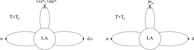
FIG. 37.: Leading contributions to flavor mixing in the $\eta-\eta^{\prime}$ system below and above the chiral phase transition.

So far, we have not discussed correlation functions related to the $U(1)_{A}$ anomaly, in particular the $\eta$ and $\eta^{\prime}$ channels. A number of authors have considered the possibility that the $U(1)_{A}$ symmetry is at least partially restored near the chiral phase transition [Shu_94, KKL_96, HW_96]. Given the fact that the $\eta^{\prime}-\pi$ mass difference is larger than all other meson mass splittings, any tendency towards $U(1)_{A}$ restoration is expected to lead to rather dramatic observable effects. Possible signatures of a hot hadronic phase with partially restored $U(1)_{A}$ symmetry that might be produced in heavy ion collisions are anomalous values of the $\eta/\pi$ and $\eta^{\prime}/\pi$ ratios, as well as an enhancement in the number of low-mass dilepton pairs from the Dalitz decay of the $\eta^{\prime}$.

In general, we know that isolated instantons disappear above the chiral phase transition. In the presence of external sources, however, isolated tunneling events can still occur, see Sec. II D 2. The density of random instantons above $T_{c}$ is expected to be $O(m^{N_{f}})$, but the contribution of isolated instantons to the expectation value of the ’t Hooft operator $\det_{f}(\bar{\psi}_{l}\psi_{R})$ (and other $U(1)_{A}$ violating operators) is of order $O(1)$ [LH_96, EHS_96]. The presence of isolated zero modes in the spectrum of the Dirac operator above $T_{c}$ can be seen explicitly in Fig. 34. The problem was studied in more detail in [Sch_96], where it was concluded that the number of (almost) zero modes above $T_{c}$ scales correctly with the dynamical quark mass and the volume.

A number of groups have measured $U(1)_{A}$ violating observables at finite temperature on the lattice. Most works focus on the the susceptibility $\chi_{\pi}-\chi_{\delta}$ [Cha_95, Boy_96, Ber_97]. Above $T_{c}$, when chiral symmetry is restored, this quantity is a measure of $U(1)_{A}$ violation. Most of the published results conclude that $U(1)_{A}$ remains broken, although recent results by the Columbia group have questioned that conclusion [Chr_96]. In any case, one should keep in mind that all results involve an extrapolations to $m=0$, and that both instanton and lattice simulations suffer from certain artefacts in this limit.

Phenomenological aspects of the $U(1)_{A}$ anomaly at finite temperature are usually discussed in terms of the effective lagrangian [PW_84]

$${\cal L} = \frac{1}{2}{\rm Tr}\left((\partial_{\mu}\Phi)(\partial_{\mu}\Phi^{\dagger})\right)-{\rm Tr}\left({\cal M}(\Phi+\Phi^{\dagger})\right)+V(\Phi\Phi^{\dagger})+c\left(\det\Phi+\det\Phi^{\dagger}\right),$$ (373)

where $\Phi$ is a meson field in the $(3,3)$ representation of $U(3)\times U(3)$, $V(\Phi\Phi^{\dagger})$ is a $U(3)\times U(3)$ symmetric potential (usually taken be quartic), ${\cal M}$ is a mass matrix and $c$ controls the strength of the $U(1)_{A}$ breaking interaction. If the coupling is chosen as $c=\chi_{top}/(12f_{\pi}^{3})$, the effective lagrangian reproduces the Witten-Veneziano relation $f_{\pi}^{2}m_{\eta^{\prime}}^{2}=\chi_{top}$. In a quenched ensemble, we can further identify $\chi_{top}\simeq(N/V)$. The temperature dependence of $c$ is usually estimated from the semi-classical tunneling amplitude $n(\rho)\sim\exp(-(8/3)(\pi\rho T)^{2})$. As a result, the strength of the anomaly is reduced by a factor $\sim 5$ near $T_{c}$. If the anomaly becomes weaker, the eigenstates are determined by the mass matrix. In that case, the mixing angle is close to the ideal value $\theta=-54.7^{\circ}$ and the non-strange $\eta_{NS}$ is almost degenerate with the pion.

FIG. 38.: Eta meson correlation functions at $T\neq 0$, normalized to free thermal correlators. Figure (a) shows the flavor singlet, (b) the octet and off-diagonal singlet-octet, (c) the non-strange and (d) the strange and off-diagonal strange-non-strange eta correlation functions. The correlators are labeled as in figure 36.

There are several points in this line of argument that are not entirely correct. The strength of the ’t Hooft term is not controlled by the topological susceptibility ($\chi_{top}=0$ in massless QCD!), $\chi_{top}$ is not proportional to the instanton density (for the same reason), and, at least below $T_{c}$, the semi-classical estimate for the instanton density is not applicable. Only above $T_{c}$ do we expect instantons to be suppressed. However, chiral symmetry restoration affects the structure of flavor mixing in the $\eta-\eta^{\prime}$ system (see Fig. 37). The mixing between the strange and non-strange eta is controlled by the light quark condensate, so $\eta_{NS}$ and $\eta_{S}$ do not mix above $T_{c}$. As a result, the mixing angle is not close to zero, as it is at $T=0$, but close to the ideal value. Furthermore, the anomaly can only affect the non-strange $\eta$, not the strange one. Therefore, if the anomaly is sufficiently strong, the $\eta_{NS}$ will be heavier than the $\eta_{S}$.

This phenomenon can also be understood from the effective lagrangian (373). The determinant is third order in the fields, so it only contributes to mass terms if some of the scalar fields have a vacuum expectation value. Above $T_{c}$, only the strange scalar has a VEV, so only light flavors mix and only the $\eta_{NS}$ receives a contribution to its mass from the anomaly. This effect was studied more quantitatively in [Sch_96]. Singlet and octet, as well as strange and non-strange eta correlation functions in the instanton liquid are shown in Fig. 38. Below $T_{c}$ the singlet correlation function is strongly repulsive, while the octet correlator shows some attraction at larger distance. The off-diagonal correlator is small and positive, corresponding to a negative mixing angle. The strange and non-strange eta correlation functions are very similar, which is a sign for strong flavor mixing. This is also seen directly from the off-diagonal correlator between $\eta_{S}$ and $\eta_{NS}$.

Above $T_{c}$, the picture changes. The off-diagonal singlet-octet correlator changes sign and its value at intermediate distances $\tau\simeq 0.5$ fm is significantly larger. The strange and non-strange eta correlators are very different from each other. The non-strange correlation function is very repulsive, but no repulsion is seen in the strange channel. This clearly supports the scenario presented above. Near $T_{c}$ the eigenstates are essentially the strange and non-strange components of the $\eta$, with the $\eta_{S}$ being the lighter of the two states. This picture is not realized completely, $\Pi_{S,NS}$ does not vanish and the singlet eta is still somewhat more repulsive than the octet eta correlation function. This is due to the fact that the light quark mass does not vanish. In particular, in this simulation the ratio $(m_{u}+m_{d})/(2m_{s})=1/7$, which is about three times larger than the physical mass ratio.

It is difficult to provide a quantitative analysis of temporal correlation functions in the vicinity of the phase transition. At high temperature the temporal direction in a euclidean box becomes short and there is no unique way to separate out the contribution from excited states. Nevertheless, under some simplifying assumptions one can try to translate the correlation functions shown in Fig. 38 into definite predictions concerning the masses of the $\eta$ and $\eta^{\prime}$. For definiteness, we will use ideal mixing above $T_{c}$ and fix the threshold for the perturbative continuum at 1 GeV. In this case, the masses of the strange and non-strange components of the $\eta$ at $T=126$ MeV are given by $m_{\eta_{S}}=(0.420\pm 0.120)$ GeV and $m_{\eta_{S}}=1.250\pm 0.400)$ GeV.

4 Screening masses

FIG. 39.: Spectrum of space-like screening masses in the instanton liquid as a function of the temperature, from [SS_96b]. The masses are given in units of the lowest fermionic Matsubara frequency $\pi T$. The dotted lines correspond to the screening masses $m=2\pi T$ and $3\pi T$ for mesons and baryons in the limit when quarks are non-interacting.

Correlation functions in the spatial direction can be studied at arbitrarily large distance, even at finite temperature. This means that (contrary to the temporal correlators) the spectrum of the lowest states can be determined with good accuracy. Although it is not directly related to the spectrum of physical excitations, the structure of space-like screening masses is of theoretical interest and has been investigated in a number of lattice [TK_87, Goc_91] and theoretical [EI_88, HZ_92, KSB_92, HSZ_94] works.

At finite temperature, the anti-periodic boundary conditions in the temporal direction require the lowest Matsubara frequency for fermions to be $\pi T$. This energy acts like a mass term for propagation in the spatial direction, so quarks effectively become massive. At asymptotically large temperatures, quarks only propagate in the lowest Matsubara mode, and the theory undergoes dimensional reduction [AP_81]. The spectrum of space-like screening states is then determined by a 3-dimensional theory of quarks with chiral mass $\pi T$, interacting via the 3-dimensional Coulomb law and the non-vanishing space-like string tension [Bor_85, MP_87].

Dimensional reduction at large $T$ predicts almost degenerate multiplets of mesons and baryons with screening masses close to $2\pi T$ and $3\pi T$. The splittings of mesons and baryons with different spins can be understood in terms of the non-relativistic spin-spin interaction. The resulting pattern of screening states is in qualitative agreement with lattice results even at moderate temperatures $T\simeq 1.5T_{c}$. The most notable exception is the pion, whose screening mass is significantly below $2\pi T$.

Screening masses in the instanton liquid are summarized in Fig. 39. First of all, the screening masses clearly show the restoration of chiral symmetry as $T\to T_{c}$: chiral partners like the $\pi$ and $\sigma$ or the $\rho$ and $a_{1}$ become degenerate. Furthermore, the mesonic screening masses are close to $2\pi T$ above $T_{c}$, while the baryonic ones are close to $3\pi T$, as expected. Most of the screening masses are slightly higher than $n\pi T$, consistent with a residual chiral quark mass on the order of 120-140 MeV. The most striking observation is the strong deviation from this pattern seen in the scalar channels $\pi$ and $\sigma$, with screening masses significantly below $2\pi T$ near the chiral phase transition. The effect disappears around $T\simeq 1.5T_{c}$. We also find that the nucleon-delta splitting does not vanish at the phase transition, but decreases smoothly.

In summary, the pattern of screening masses seen in the instanton liquid is in agreement with the results of lattice calculations. In particular, the attractive interaction provided by instanton molecules accounts for the fact that the $\pi,\sigma$ screening masses are much smaller than $2\pi T$ near $T_{c}$.

D Instantons at finite temperature: lattice studies

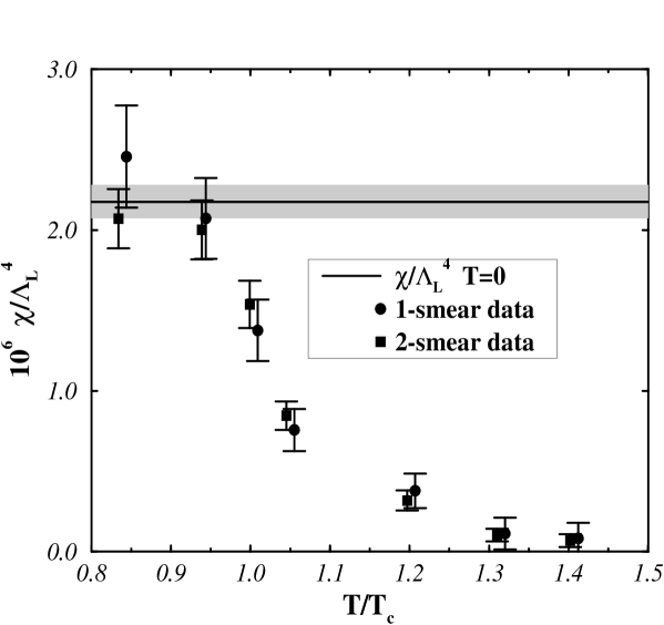
FIG. 40.: Lattice measurements of the temperature dependence of the topological susceptibility in pure gauge $SU(3)$, from (a)[CS_95] and (b) [ADD_96]. The dash-dotted line labeled P-Y in Fig. (a) corresponds to the semi-classical (Pisarski-Yaffe) result (332), while the dashed curve shows the rescaled formula discussed in the text. The solid line labeled PCAC is not very relevant for pure gauge theory. In Fig. (b), the circles and squares correspond to two different topological charge operators.

Very few lattice simulations have focused on the role of instantons at finite temperature, and all the results that have been reported were obtained in the quenched approximation [Tep_86, HTW_87, CS_95, IMM_95]. In this section we will concentrate on results obtained by the cooling method, in particular [CS_95]. In this work, the temperature was varied by changing the number of time slices $N_{\tau}=2,4,\ldots,16$, while the spatial extent of the lattice and the coupling constant $\beta=6$ were kept fixed.

The topological susceptibility was calculated from topological charge fluctuations $\langle Q^{2}\rangle/V$ in the cooled configurations. In the quenched theory, correlations between instantons are not very important, and the topological susceptibility provides a good estimate of the instanton density. Figure 40a shows their results as a function of $T$. At $T=0$, $\chi_{top}\simeq(180\,{\rm MeV})^{4}$, in agreement with the phenomenological value. The topological susceptibility is almost temperature independent below the critical temperature ($T_{c}\simeq 260$ MeV in quenched QCD), but drops very fast above $T_{c}$. The temperature dependence of $\chi_{top}$ above $T_{c}$ is consistent with the Debye-screening suppression factor (332), but with a shifted temperature, $T^{2}\to(T^{2}-T_{c}^{2})$. Clearly, these results support the arguments presented in Sec. VII A 3. The conclusions of Chu and Schramm are consistent with results reported in [IMM_95, ADD_96]. We show the results of Alles et al. in Fig. 40b.

Chu and Schramm also extracted the average instanton size from the correlation function of the topological charge density. Below $T_{c}$, they find $\rho=0.33$ fm independent of temperature while at $T=334$ MeV, they get a smaller value $\rho=0.26$ fm. This result is in good agreement with the Debye-screening dependence discussed above.

Finally, they considered instanton contributions to the pressure and space-like hadronic wave functions. They find that instantons contribute roughly 15% of the pressure at $T=334$ MeV and 5% at $T=500$ MeV. While space-like hadronic wave functions are dominated by instantons at $T=0$ (see Sec. VI G), this is not true at $T>T_{c}$. This is consistent with the idea that space-like wave functions above $T_{c}$ are determined by the space-like string tension [KSB_92], which disappears during cooling.

Clearly, studies with dynamical fermions are of great interest. Some preliminary results have been obtained by Ilgenfritz et al. (private communication). Using a “gentle cooling” algorithm with only a few cooling iterations in order to prevent instantons and anti-instantons from annihilating each other, they found evidence for an anticorrelation of topological charges in the time direction above $T_{c}$. This would be the first direct lattice evidence for the formation of polarized instanton molecules in the chirally symmetric phase.

VIII Instantons in related theories

A Two-dimensional theories

Although two-dimensional theories should logically be placed between the simplest quantum mechanical systems and Yang-Mills theories, we have postponed their discussion up to now in order not to disrupt the main line of the review. Nevertheless, topological objects play an important role in many low dimensional models. We do not want to give an exhaustive survey of these theories, but have selected two examples, the $O(2)$ and $O(3)$ models, which, in our opinion, provide a few interesting lessons for QCD. As far as other theories are concerned, we refer the reader to the extensive literature, in particular on the Schwinger model [Smi_94a, SSZ_95] and two dimensional QCD with fundamental or adjoint fermions [Smi_94b].

1 The $O(2)$ sigma model

The $O(2)$ model is also known as a the $d=2$ Heisenberg magnet or the $XY$ model. It describes a two dimensional spin vector $\vec{S}$ governed by the Hamiltonian

$$\frac{E}{T} = \frac{1}{2t}\int d^{2}x\,\left(\partial_{\mu}\vec{S}\right)^{2},$$ (374)

together with the constraint ${\vec{S}}^{2}=1$. Here, $t=T/J$ is a dimensionless parameter, and $J$ the coupling constant. In this section we will follow the more traditional language of statistical mechanics rather than euclidean quantum field theory. This means that the coordinates are $x,y$ and the weight factor in the functional integral is $\exp(-E/T)$. Of course, one can always switch to field theory language by replacing the energy by the action and the temperature by the coupling constant $g^{2}$.

The statistical sum is Gaussian except for the constraint. We can make this more explicit by parameterizing the two dimensional spin vector $\vec{S}$ in the form $S_{1}=\cos\theta,\,S_{2}=\sin\theta$. In this case, the energy is given by $E/T=\frac{1}{2t}\int d^{2}x\,(\partial_{\mu}\theta)^{2}$, which would describe a non-interacting scalar field if it were not for the fact that $\theta$ is a periodic variable. It is often useful to define the theory directly on the lattice. The partition function is given by

$$Z = \int\left(\prod_{x}\frac{d\theta_{x}}{2\pi}\right)\,\exp\left(\beta\sum_{x,\hat{e}_{\mu}}\left[\cos(\theta_{x}-\theta_{x+\hat{e}_{\mu}})-1\right]\right),$$ (375)

which is automatically periodic in $\theta$. The lattice spacing $a$ provides an ultraviolet cutoff. We should also note that the $O(2)$ model has a number of physical applications. First of all, the model obviously describes a two dimensional magnet. In addition to that, fluctuations of the order parameter in superconducting films of liquid ⁴He and the dynamics of dislocations in the melting of two-dimensional crystals are governed by effective $O(2)$ models.

A two dimensional theory with a continuous symmetry cannot have an ordered phase at non-zero temperature. This means that, under ordinary circumstances, two dimensional models cannot have a phase transition at finite temperature [MW_66]. The $O(2)$ model is special because it has a phase transition at $T_{c}\simeq(\pi J)/2>0$ (although, in agreement with the Mermin-Wagner theorem, the transition is not characterized by a local order parameter). Both the low and the high temperature phase are disordered, but the functional form of the spin correlation function $K(x)=\langle\vec{S}(x)\vec{S}(0)\rangle$ changes. In some sense, the whole region $T<T_{c}$ is critical because the correlation functions exhibits a power-law decay [Ber_71]. For $T>T_{c}$ the spin correlator decays exponentially, and the theory has a mass gap.

The mechanism of this phase transition was clarified in the seminal paper by [KT_73], see also the review [Kog_79]. Let us start with the low temperature phase. In terms of the angle variable $\theta$, the spin correlation function is given by

$$K(x) = N^{-1}\int d\theta(x)\,e^{i\theta(x)}e^{-i\theta(0)}e^{-1/(2t)\int d^{2}x(\partial_{\mu}\theta)^{2}}.$$ (376)

At small temperature, the system is dominated by spin waves and we expect that fluctuations in $\theta$ are small. In this case we can ignore the periodic character of $\theta$ for the moment. Using the propagator for the $\theta$-field, $G(r)=-1/(2\pi)\log(r/a)$, we have

$$K(r) = \exp(tG(r))\,\sim\,r^{-\frac{t}{2\pi}}.$$ (377)

The correlator shows a power law, with a temperature-dependent exponent $\eta=T/(2\pi J)$.

In order to understand the phase transition in the $O(2)$ model, we have to go beyond Gaussian fluctuations and include topological objects. These objects can be classified by a winding number

$$q = \frac{1}{2\pi}\oint d\vec{x}\cdot\vec{\nabla}\theta.$$ (378)

Solutions with $q=\pm 1$ are called (anti) vortices. A solution with $q=n$ is given by $\theta=n\alpha$ with $\alpha=\arctan(y/x)$. The energy of a vortex is

$$\frac{E(q=1)}{T} = \frac{\pi}{t}\int\frac{dr}{r}\left(\frac{\partial\theta}{\partial\alpha}\right)^{2}\;=\;\frac{\pi n^{2}}{t}\log(R/a),$$ (379)

where $R$ is the IR cutoff. Since the energy is logarithmically divergent, one might think that vortex configurations are irrelevant. In fact, they are crucial for the dynamics of the phase transition.

The reason is that it is not the energy, but the free energy $F=E-TS$ which is relevant for the statistical sum. The entropy of an isolated vortex is essentially the logarithm of all possible vortex positions, given by $S=\log[(R/a)^{2}]$. For temperatures $T>T_{c}\simeq(\pi J)/2$, entropy dominates over energy and vortices are important. The presence of vortices implies that the system is even more disordered and the spin correlator decays exponentially.

What happens to the vortex gas below $T_{c}$? Although isolated vortices have infinite energy, vortex-anti-vortex pairs (molecules) have finite energy $E\simeq\pi/(2t)[\log(R/a)+{\rm const}]$, where $R$ is the size of the molecule. At low temperature, molecules are strongly suppressed, but as the temperature increases, they become more copious. Above the critical temperature, molecules are ionized and a vortex plasma is formed.

There is yet another way to look at this transition. We can decompose any field configuration into the contribution of vortices and a smooth field. Using this decomposition, one can see that the $O(2)$ sigma model is equivalent to a two dimensional Coulomb gas. The Koesterlitz-Thouless transition describes the transition from a system of dipoles to an ionized plasma. The correlation length of the spin system is nothing but the Debye screening length in the Coulomb plasma. At the transition point, the screening length has an essential singularity [KT_73]

$$\xi\sim\exp\left(\frac{\rm const}{|T-T_{c}|^{1/2}}\right)$$ (380)

rather than the power law divergence observed in ordinary phase transitions.

There is an obvious lesson we would like to draw from this: the two phases of the $O(2)$ model resemble the two phases found in QCD (Sec. VII B 4). In both cases the system is described by an (approximately) random ensemble of topological objects in one phase, and by bound pairs of pseudo-particles with opposite charge in the other. The only difference is that the high and low temperature phase are interchanged. This is essentially due to the fact that temperature has a different meaning in both problems. In the $O(2)$ model, instantons are excited at high temperature, while in QCD they are suppressed.

2 The $O(3)$ sigma model

The $O(2)$ model can be generalized to a $d=2$ spin system with a three (or, more generally, $N$) dimensional spin vector $\vec{S}$ of unit length. Unlike the $O(2)$ model, the $O(3)$ model is not just a free field theory for a periodic variable. In fact, in many ways the model resembles QCD much more than the $O(2)$ model does. First of all, for $N>2$ the rotation group is non-abelian and spin waves (with $(N-1)$ polarizations) interact. In order to treat the model perturbatively, it is useful to decompose the vector field in the form $\vec{S}=(\sigma,\vec{\pi})$, where $\vec{\pi}$ is an $(N-1)$ dimensional vector field and $\sigma=\sqrt{1-{\vec{\pi}}^{2}}$. The perturbative analysis of the $O(N)$ model gives the beta function [Pol_75]

$$\beta(t) = -\frac{N-2}{2\pi}t^{2}+O(t^{3}),$$ (381)

which shows that just like QCD, the $O(N)$ model is asymptotically free for $N>2$. In the language of statistical mechanics, the beta function describes the evolution of the effective temperature as a function of the scale. A negative beta function then implies that if the temperature is low at the atomic scale $a$, the effective temperature grows as we go to larger scales. Eventually, the reduced temperature is $t=O(1)$ ($T$ is comparable to $J$), fluctuations are large and long range order is destroyed. Unlike the $N=2$ model, the $O(3)$ model has only one critical point, $t=0$, and correlation functions decay exponentially for all temperatures $T>0$.

Furthermore, like non-abelian gauge theory, the $O(3)$ model has classical instantons solutions. The topology is provided by the fact that field configurations are maps from two dimensional space-time (compactified to a sphere) into another sphere which describes the orientation of $\vec{S}$. The winding number is defined by

$$q = \frac{1}{8\pi}\int d^{2}x\,\epsilon_{\mu\nu}\vec{S}\cdot(\partial_{\mu}\vec{S}\times\partial_{\nu}\vec{S}).$$ (382)

Similar to QCD, solutions with integer winding number and energy $E=4\pi J|q|$ can be found from the self-duality equation

$$\partial_{\mu}\vec{S} = \pm\epsilon_{\mu\nu}\vec{S}\times\partial_{\nu}\vec{S}.$$ (383)

A solution with $q=1$ can be constructed by means of the stereographic projection

$$\vec{S} = \left(\frac{2\rho x_{1}}{x^{2}+\rho^{2}},\frac{2\rho x_{2}}{x^{2}+\rho^{2}},\frac{x^{2}-\rho^{2}}{x^{2}+\rho^{2}}\right).$$ (384)

At large distances all spins point up, in the center the spin points down, and at intermediate distances $x\sim\rho$ all spins are horizontal, pointing away from the center. Like QCD, the theory is scale invariant on the classical level and the energy of an instanton is independent of the size $\rho$. Instantons in the $O(2)$ model are sometimes called Skyrmions, in analogy with the static (three-dimensional) solitons introduced by Skyrme in the $d=4$ $O(4)$ model [Sky_61].

The next logical step is the analog of the ’t Hooft calculation of fluctuations around the classical instanton solution. The result of the semi-classical calculation is [Pol_75]

$$dN_{inst}\sim{d^{2}xd\rho\over\rho^{3}}\exp(-E/T)\sim{d^{2}xd\rho\over\rho}$$ (385)

which is divergent both for large and small radii. The result for large $\rho$ is of course not reliable, since it is based on the one-loop beta function.

Because the $O(3)$ model shows so many similarities with QCD, it is natural to ask whether one can learn anything of relevance for QCD. Indeed, the $O(3)$ model has been widely used as a testing ground for new methods in lattice gauge theory. The numerical results provide strong support for the renormalization group analysis. For example, [CEP_95] studied the $O(3)$ model at correlation lengths as large as $\xi/a\sim 10^{5}$! The results agree with state-of-the-art theoretical predictions (based on the 3-loop beta function and an overall constant determined from the Bethe ansatz) with a very impressive accuracy, on the order of few percent.

Unfortunately, studies of instantons in the $O(3)$ model have not produced any significant insights. In particular, there are no indications that small-size (semi-classical) instantons play any role in the dynamics of the theory. Because of the divergence in the instanton density, the topological susceptibility in the $O(3)$ has no continuum limit. This conclusion is supported by lattice simulations [MS_94]. The simulations also indicate that for large size instantons, the size distribution is $dN\sim d\rho/\rho^{-3}$. This power differs from the semi-classical result, but it agrees with the $\rho$ dependence coming from the Jacobian alone, without the running coupling in the action. This result supports the idea of a frozen coupling constant discussed in Sec. III C 3.

B Instantons in electroweak theory

In the context of this review we cannot provide a detailed discussion of instantons and baryon number violation in electroweak theory. Nevertheless, we briefly touch on this subject, because electroweak theory provides an interesting theoretical laboratory. The coupling constant is small, the instanton action is large and the semi-classical approximation is under control. Unfortunately, this means that under ordinary conditions tunneling events are too rare to be of physical importance. Interesting questions arise when one tries to increase the tunneling rate, e.g. by studying scattering processes with collision energies close to the barrier height, or processes in the vicinity of the electroweak phase transition. Another interesting problem is what happens if we consider the Higgs expectation value to be a free parameter. When the Higgs VEV is lowered, electroweak theory becomes a strongly interacting theory, and we encounter many of the problems we have to deal with in QCD.

Electroweak theory is an $SU(2)_{L}\times U(1)$ chiral gauge theory coupled to a Higgs doublet. For simplicity we will neglect the $U(1)$ interactions in the following, i.e. set the Weinberg angle to zero. The most important difference as compared to QCD is the fact that gauge invariance is spontaneously broken. In the ground state, the Higgs field acquires an expectation value, which gives masses to the $W$ bosons as well as to the quarks and charged leptons. If the Higgs field has a non-zero VEV the instanton is, strictly speaking, not a solution of the equations of motion. Nevertheless, it is clear that if $\rho\ll v^{-1}$ (where $v$ is the Higgs VEV), the gauge fields are much stronger than the Higgs field and there should be an approximate instanton solution. In the central region $x<m_{W}^{-1},m_{H}^{-1}$, the solution can be found by keeping the instanton gauge field fixed and solving the equations of motion for the Higgs field. The result is

$$\phi = \frac{x^{2}}{x^{2}+\rho^{2}}U\left(0\atop{v/\sqrt{2}}\right),$$ (386)

where $U$ is the color orientation matrix of the instanton. The result shows that the instanton makes a hole of size $\rho$ in the Higgs condensate. Scale invariance is lost and the instanton action depends on the Higgs VEV [tHo_76b]

$$S = {8\pi^{2}\over g^{2}}+2\pi^{2}\rho^{2}v^{2}.$$ (387)

The tunneling rate is $p\sim\exp(-S)$ and large instantons with $\rho\gg v^{-1}$ are strongly suppressed.

The loss of scale invariance also implies that in electroweak theory, the height of the barrier separating different topological vacua can be determined. There is a static solution with winding number 1/2, corresponding to the top of the barrier, called the sphaleron [KM_84]. The sphaleron energy is $E_{sph}\simeq 4m_{W}/\alpha_{W}\simeq 10$ TeV.

Elektroweak instantons also have fermionic zero modes, and as usual the presence of these zero modes is connected with the axial anomaly. Since only left-handed fermions participate in weak interactions, both vector and axial-vector currents are not conserved. The ’t Hooft vertex contains all 12 weak doublets

$$(\nu_{e},e),\;(\nu_{\mu},\mu),\;(\nu_{\tau},\tau),\;3*(u,d),\;3*(c,s),\;3*(t,b),$$ (388)

where the factors of three come from color. Each doublet provides one fermionic zero mode, the flavor depending on the isospin orientation of the instanton. The ’t Hooft vertex violates both baryon and lepton number. These processes are quite spectacular, because all families have to be involved, for example

$$u+d \rightarrow \bar{d}+\bar{s}+2\bar{c}+3\bar{t}+e^{+}+\mu^{+}+\tau^{+},$$ (389)

$$u+d \rightarrow \bar{u}+2\bar{s}+\bar{c}+\bar{t}+2\bar{b}+\nu_{e}+\nu_{\mu}+\tau^{+}.$$ (390)

Note that $\Delta B=\Delta L=-3$, so $B+L$ is violated, but $B-L$ is conserved. Unfortunately, the probability of such an event is tiny, proportional to the square of the tunneling amplitude $P\sim\exp(-16\pi^{2}/g^{2}_{w})\sim 10^{-169}$ [tHo_76], many orders of magnitude smaller than any known radioactive decay.

Many authors have discussed the possibility of increasing the tunneling rate by studying processes near the electroweak phase transition [KRS_85] or scattering processes involving energies close to the sphaleron barrier $E\simeq E_{sph}$. Since $E_{sph}\simeq 10$ TeV, this energy would have been accessible at the SSC and will possibly be within reach at the LHC. The latter idea became attractive when it was realized that associated multi-Higgs and $W$ production increases the cross section [Rin_90, Esp_90]. On general grounds one expects

$$\sigma_{\Delta(B+L)} \sim \exp\left[-\frac{4\pi}{\alpha_{W}}F\left(\frac{E}{E_{sph}}\right)\right],$$ (391)

where $F(\epsilon)$ is called the “holy grail” function. At low energy, $F(0)=1$ and baryon number violation is strongly suppressed. The first correction is $F(\epsilon)=1-\frac{9}{8}\epsilon^{4/3}+O(\epsilon^{2})$, indicating that the cross section rises with energy. Clearly, the problem is the behavior of $F(\epsilon)$ near $\epsilon=1$. Most authors now seem to agree that $F(\epsilon)$ will not drop below $F\simeq 1/2$, implying that baryon number violation in $pp$ collisions will remain unobservable [Zak_92, MS_92, MS_92b, Ven_92, DP_94]. The question is of interest also for QCD, because the holy grail function at $\epsilon=1$ is related to the instanton-anti-instanton interaction at short distance. In particular, taking into account unitarity in the multi-$W$ (or multi-gluon) production process correspond to an effective instanton-anti-instanton repulsion, see Sec. IV A 1.

The other question of interest for QCD is what happens if the Higgs VEV $v$ is gradually reduced. As $v$ becomes smaller the theory moves from the weak-coupling to the strong-coupling regime. The vacuum structure changes from a very dilute system of $IA$ molecules to a more dense (and more interesting) non-perturbative vacuum. Depending on the number of light fermions, one should eventually reach a confining, QCD-like phase. In this phase, leptons are composite but the low-energy effective action is probably similar to the one in the Higgs phase [AF_81, CFJ_86]. Unfortunately, the importance of non-perturbative effects has never been studied.

Let us comment only on one element which is absent in QCD, the scalar-induced interaction between instantons. Although the scalar interaction is order $O(1)$ and therefore suppressed with respect to the gauge interaction $O(g^{-2})$, it is long range if the Higgs mass is small. For $m_{H}^{-1}\gg R\gg\rho$ the $IA$ interaction is [Yun_88]

$$S_{Higgs}=4\pi^{2}a^{2}\rho^{2}\left[1+\frac{\rho^{2}}{R^{2}}\left(2(u\cdot\hat{R})^{2}-1\right)\right]+O\left(\frac{1}{R^{4}}\right)$$ (392)

Unlike the gluonic dipole interaction, it does not vanish if averaged over all orientations, $\langle(u\cdot\hat{R})^{2}\rangle=1/4$. This means that the scalar interaction can provide coherent attraction for distances $Rm_{H}<1$, which is of the order $v^{2}\rho^{4}n/m_{H}^{2}$ where $n$ is the instanton density. This is large if the Higgs mass is small.

Another unusual feature of Yung interaction (392) is that it is repulsive for $u\cdot\hat{R}=1$ (which is the most attractive orientation for the dipole interaction). This would suggest that for a light Higgs mass, there is no small $R$ problem. This question was studied in [VS_93]. For the complete Yung ansatz (which is a good approximation to the full streamline solution) the approximate result (392) is only valid for $R>10\rho$, while for smaller separation the dependence on $u\cdot\hat{R}$ is reversed.

C Supersymmetric QCD

Supersymmetry (SUSY) is a powerful theoretical concept which is of great interest in constructing field theories beyond the standard model. In addition to that, supersymmetric field theories provide a very useful theoretical laboratory, and a number of important advances in understanding the ground state of strongly interacting gauge theories. We have already seen one example for the usefulness of supersymmetry in isolating instanton effects in the context of SUSY quantum mechanics, Sec. II B. In that case, SUSY implies that perturbative contributions to the vacuum energy vanish and allows a precise definition of the instanton-anti-instanton contribution. In the following, we will see that supersymmetry can be used in very much the same way in the context of gauge field theories.

In general, one should keep in mind that SUSY theories are just ordinary field theories with a very specific matter content and certain relations between different coupling constants. Eventually, we hope to understand non-abelian gauge theories for all possible matter sectors. In particular, we want to know how the structure of the theory changes as one goes from QCD to it supersymmetric generalizations, where many exact exact statements about instantons and the vacuum structure are known. Deriving these results often requires special techniques that go beyond the scope of this review. For details of the supersymmetric instanton calculus we refer the reader to the extensive review [AKM_88]. Nevertheless, we have tried to include a number of interesting results and explain them in standard language.

As theoretical laboratories SUSY theories have several advantages over ordinary field theories. We have already mentioned one of them: Non-renormalization theorems imply that many quantities do not receive perturbative contributions, so instanton effects are more easily identified. In addition to that, SUSY gauge theories usually have many degenerate classical vacua. These degeneracies cannot be lifted to any order in perturbation theory, and instantons often play an important role in determining the ground state. In most cases, the classical vacua are characterized by scalar field VEVs. If the scalar field VEV is large, one can perform reliable semi-classical calculations. Decreasing the scalar VEV, one moves towards strong coupling and the dynamics of the theory is non-trivial. Nevertheless, supersymmetry restricts the functional dependence of the effective potential on the scalar VEV (and other parameters, like masses or coupling constants), so that instanton calculations can often be continued into the strong coupling domain.

Ultimately, we would like to understand the behavior of SUSY QCD as we introduce soft supersymmetry breaking terms and send the masses of the gluinos and squarks to infinity. Not much progress has been achieved in this direction, but at least for small breaking the calculations are feasible and some lessons have been learned.

1 The instanton measure and the perturbative beta function

The simplest ($N=1$) supersymmetric non-abelian gauge theory is $SU(2)$ SUSY gluodynamics, defined by

$${\cal L} = -\frac{1}{4g^{2}}F_{\mu\nu}^{a}F^{a}_{\mu\nu}+\frac{i}{2g^{2}}\lambda^{a}(D\!\!\!\!/\,)_{ab}\lambda^{b}$$ (393)

where the gluino field $\lambda^{a}$ is a Majorana fermion in the adjoint representation of $SU(2)$. More complicated theories can be constructed by adding additional matter fields and scalars. $N$ extended supersymmetry has $N$ gluino fields as well as additional scalars. Clearly, supersymmetric gluodynamics has $\theta$ vacua and instanton solutions. The only difference as compared to QCD is that the fermions carry adjoint color, so there are twice as many fermion zero modes. If the model contains scalars fields that acquire a vacuum expectation value, instantons are approximate solutions and the size integration is automatically cut off by the scalar VEV. These theories usually resemble electroweak theory more than they do QCD.

At first glance, instanton amplitudes seem to violate supersymmetry: the number of zero modes for gauge fields and fermions does not match, while scalars have no zero modes at all. However, one can rewrite the tunneling amplitude in manifestly supersymmetric form [NSVZ_83b]. We will not do this here, but stick to the standard notation. The remarkable observation is that the determination of the tunneling amplitude in SUSY gauge theory is actually simpler than in QCD. Furthermore, with some additional input, one can determine the complete perturbative beta function from the tunneling amplitude.

The tunneling amplitude is given by

$$n(\rho)\sim\exp\left(-\frac{2\pi}{\alpha}\right)M^{n_{g}-n_{f}/2}\left(\frac{2\pi}{\alpha}\right)^{n_{g}/2}d^{4}x\frac{d\rho}{\rho^{5}}\rho^{k}\prod_{f}d^{2}\xi_{f},$$ (394)

where all factors can be understood from the ’t Hooft calculation discussed in Sec. II C 4. There are $n_{g}=4N_{c}$ bosonic zero modes that have to be removed from the determinant and give one power of the regulator mass $M$ each. Similarly, each of the $n_{f}$ fermionic zero modes gives a factor $M^{1/2}$. Introducing collective coordinates for the bosonic zero modes gives a Jacobian $\sqrt{S_{0}}$ for every zero mode. Finally, $d^{2}\xi$ is the integral over the fermionic collective coordinates and $\rho^{k}$ is the power of $\rho$ needed to give the correct dimension. Supersymmetry now ensures that all non-zero mode contributions exactly cancel. More precisely, the subset of SUSY transformations which does not rotate the instanton field itself, mixes fermionic and bosonic modes non-zero modes but annihilates zero modes. This is why all non-zero modes cancel but zero modes can be unmatched. Note that as a result of this cancellation, the power of $M$ in the tunneling amplitude is an integer.

Renormalizability demands that the tunneling amplitude is independent of the regulator mass. This means that the explicit $M$-dependence of the tunneling amplitude and the $M$ dependence of the bare coupling have to cancel. As in QCD, this allows us to determine the one-loop coefficient of the beta function $b=(4-N)N_{c}-N_{f}$. Again note that $b$ is an integer, a result that would appear very mysterious if we did not know about instanton zero modes.

In supersymmetric theories one can even go one step further and determine the beta function to all loops [NSVZ_83b, VZNS_86]. For that purpose let us write down the renormalized instanton measure

$$n(\rho)\sim\exp\left(-\frac{2\pi}{\alpha}\right)M^{n_{g}-n_{f}/2}\left(\frac{2\pi}{\alpha_{R}}\right)^{n_{g}/2}Z_{g}^{n_{g}/2}\left(\prod_{f}Z_{f}^{-1/2}\right)d^{4}x\frac{d\rho}{\rho^{5}}\rho^{k}\prod_{f}d^{2}\xi_{f},$$ (395)

where we have introduced the field renormalization factors $Z_{g,f}$ for the bosonic/fermionic fields. Again, non-renormalization theorems ensure that the tunneling amplitude is not renormalized at higher orders (the cancellation between the non-zero mode determinants persists beyond one loop). For gluons the field renormalization (by definition) is the same as the charge renormalization $Z_{g}=\alpha_{R}/\alpha_{0}$. Furthermore, supersymmetry implies that the field renormalization is the same for gluinos and gluons. This means that the only new quantity in (395) is the anomalous dimension of the quark fields, $\gamma_{\psi}=d\log Z_{f}/d\log M$.

Again, renormalizability demands that the amplitude is independent of $M$. This condition gives the NSVZ beta function [NSVZ_83b] which, in the case $N=1$, reads

$$\beta(g) = -\frac{g^{3}}{16\pi^{2}}\frac{3N_{c}-N_{f}+N_{f}\gamma_{\psi}(g)}{1-N_{c}g^{2}/8\pi^{2}}.$$ (396)

The anomalous dimension of the quarks has to be calculated perturbatively. To leading order, it is given by

$$\gamma_{\psi}(g) = -\frac{g^{2}}{8\pi^{2}}\frac{N_{c}^{2}-1}{N_{c}}+O(g^{4}).$$ (397)

The result (396) agrees with explicit calculations up to three loops [JJN_97]. Note that the beta function is scheme dependent beyond two loops, so in order to make a comparison with high order perturbative calculations, one has to translate from the Pauli-Vilars scheme to a more standard perturbative scheme, e.g. $\overline{MS}$.

In theories without quarks, the NSVZ result determines the beta function completely. For $N$-extended supersymmetric gluodynamics, we have

$$\beta(g) = -\frac{g^{3}}{16\pi^{2}}\frac{N_{c}(4-N)}{1-(2-N)N_{c}g^{2}/(8\pi^{2})}.$$ (398)

One immediately recognizes two interesting special cases. For $N=4$, the beta function vanishes and the theory is conformal. In the case $N=2$, the denominator vanishes and the one loop result for the beta function is exact.

2 $N=1$ supersymmetric QCD

In the previous section we used instantons only as a tool to simplify a perturbative calculation. Naturally, the next question is whether instantons cause important dynamical effects in SUSY theories. Historically, there has been a lot of interest in SUSY breaking by instantons, first discovered in the quantum mechanical model discussed in Sec. II B. The simplest field theory in which SUSY is broken by instantons is the $SU(2)\times SU(3)$ model [ADS_84c, ADS_85, VZS_85]. However, non-perturbative SUSY breaking does not take place in supersymmetric QCD, and we will not discuss this phenomenon any further.

An effect which is more interesting in our context is gluino condensation in SUSY gluodynamics (393) [NSV_83]. For $SU(2)$ color, the gluino condensate is most easily determined from the correlator $\langle\lambda^{a}_{\alpha}\lambda^{a\,\alpha}(x)\lambda^{b}_{\beta}\lambda^{b\,\beta}(0)\rangle$. In $SU(N)$, one has to consider the $N$-point function of $\lambda^{a}_{\alpha}\lambda^{a\,\alpha}$. In supersymmetric theories, gluinos have to be massless, so the tunneling amplitude is zero. However, in the $N$-point correlation function all zero modes can be absorbed by external sources, similar to the axial anomaly in QCD. Therefore, there is a non-vanishing one-instanton contribution. In agreement with SUSY Ward-identities, this contribution is $x$-independent. Therefore, one can use cluster decomposition to extract the gluino condensate $\langle\lambda\lambda\rangle=\pm A\Lambda^{3}$ (in $SU(2)$), where $A$ is a constant that is fixed from the single instanton calculation.

There are a number of alternative methods to calculate the gluino condensate in SUSY gluodynamics. For example, it has been suggested that $\langle\lambda\lambda\rangle$ can be calculated directly using configurations with fractional charge [CG_84]. In addition to that, one can include matter fields, make the theory Higgs-like, and then integrate out the matter fields [NSV_83b, SV_88b]. This method gives a different numerical coefficient for the gluino condensate, a problem that was recently discussed in [KS_97].

The next interesting theory is $N=1$ SUSY QCD, where we add $N_{f}$ matter fields (quarks $\psi$ and squarks $\phi$) in the fundamental representation. Let us first look at the NSVZ beta function. For $N=1$, the beta function blows up at $g^{2}_{*}=8\pi^{2}/N_{c}$, so the renormalization group trajectory cannot be extended beyond this point. Recently, Kogan and Shifman suggested that at this point the standard phase meets the renormalization group trajectory of a different (non-asymptotically free) phase of the theory [KS_95]. The beta function vanishes at $g^{2}_{*}/(8\pi^{2})=[N_{c}(3N_{c}-N_{f})]/[N_{f}(N_{c}^{2}-1)]$, where we have used the one-loop anomalous dimension. This is reliable if $g_{*}$ is small, which we can ensure by choosing $N_{c}\to\infty$ and $N_{f}$ in the conformal window $3N_{c}/2<N_{f}<3N_{c}$. Recently, Seiberg showed that the conformal point exists for all $N_{f}$ in the conformal window (even if $N_{c}$ is not large) and clarified the structure of the theory at the conformal point [Sei_94].

Let us now examine the vacuum structure of SUSY QCD for $N_{c}=2$ and $N_{f}=1$. In this case we have one Majorana fermion (the gluino), one Dirac fermion (the quark) and one scalar squark (or Higgs) field. The quark and squark fields do not have to be massless. We will denote their mass by $m$, while $v$ is the vacuum expectation value of the scalar field. In the semi-classical regime $v\gg\Lambda$, the tunneling amplitude (395) is $O(\Lambda^{5})$. The ’t Hooft effective lagrangian is of the form $\lambda^{4}\psi^{2}$, containing four quark and two gluino zero modes. As usual, instantons give an expectation value to the ’t Hooft operator. However, due to the presence of Yukawa couplings and a Higgs VEV, they can also provide expectation values for operators with less than six fermion fields. In particular, combining the quarks with a gluino and a squark tadpole we can construct a two gluino operator. Instantons therefore lead to gluino condensation [ADS_84b]. Furthermore, using two more Yukawa couplings one can couple the gluinos to external quark fields. Therefore, if the quark mass is non-zero we get a finite density of individual instantons $O(m\Lambda^{5}/v^{2})$, see Fig. 41.

FIG. 41.: Instanton contributions to the effective potential in supersymmetric QCD.

As in ordinary QCD, there are also instanton-anti-instanton molecules. The contribution of molecules to the vacuum energy can be calculated either directly or indirectly, using the single instanton result and arguments based on supersymmetry. This provides a nice check on the direct calculation, because in this case we have a rigorous definition of the contribution from molecules. Calculating the graph shown in Fig. 41b, one finds [Yun_88]

$$\epsilon^{IA}_{vac} = \frac{32\Lambda^{10}}{g^{8}v^{6}},$$ (399)

which agrees with the result originally derived in [ADS_84b] using different methods. The result implies that the Higgs expectation value is driven to infinity and $N_{f}=1$ SUSY QCD does not have a stable ground state. The vacuum can be stabilized by adding a mass term. For non-zero quark mass $m$ the vacuum energy is given by

$$\epsilon_{vac} = 2m^{2}v^{2}-\frac{16m\Lambda^{5}}{g^{4}v^{2}}+\frac{32\Lambda^{10}}{g^{8}v^{6}}\;=\;2\left(mv-\frac{4\Lambda^{5}}{g^{4}v^{3}}\right)^{2}$$ (400)

where the first term is the classical Higgs mass term, the second is the one-instanton contribution and the third is due to molecules. In this case, the theory has a stable ground state at $v^{2}=\pm 2\Lambda^{5/2}/(g^{2}m^{1/2})$. Since SUSY is unbroken, the vacuum energy is exactly zero. Let us note that in the semi-classical regime $m\ll\Lambda\ll v$ everything is under control: instantons are small $\rho\sim v^{-1}$, individual instantons are rare, molecules form a dilute gas, $nR^{4}\sim(v/\Lambda)^{10}$, and the instanton and anti-instanton inside a molecule are well separated, $R_{IA}/\rho\sim 1/\sqrt{g}$. Supersymmetry implies that the result remains correct even if we leave the semi-classical regime. This means, in particular, that all higher order instanton corrections ($O(\Lambda^{15})$ etc.) have to cancel exactly. Checking this explicitly might provide a very non-trivial check of the instanton calculus.

Recently, significant progress has been made in determining the structure of the ground state of $N=1$ supersymmetric QCD for arbitrary $N_{c}$ and $N_{f}$ [IS_95]. Seiberg showed that the situation discussed above is generic for $N_{f}<N_{c}$: A stable ground state can only exist for non-zero quark mass. For $N_{f}=N_{c}-1$ the $m\neq 0$ contribution to the potential is an instanton effect. In the case $N_{f}=N_{c}$, the theory has chiral symmetry breaking (in the chiral limit $m\to 0$) and confinement. For $N_{f}=N_{c}+1$, there is confinement but no chiral symmetry breaking. Unlike QCD, the ’t Hooft anomaly matching conditions can be satisfied with massless fermions. These fermions can be viewed as elementary fields in the dual (or “magnetic”) formulation of the theory. For $N_{c}+1<N_{f}<3N_{c}/2$ the magnetic formulation of the theory is IR free, while for $3N_{c}/2<N_{f}<3N_{c}$ the theory has an infrared fixed point. Finally, for $N_{f}>3N_{c}$, asymptotic freedom is lost and the electric theory is IR free.

3 $N=2$ supersymmetric gauge theory

The work of Seiberg has shown that supersymmetry sufficiently constrains the effective potential in $N=1$ supersymmetric QCD so that the possible vacuum states for all $N_{c}$ and $N_{f}$ can be determined. For $N=2$ extended supersymmetric QCD, these constraints are even more powerful. Witten and Seiberg have been able to determine not just the effective potential, but the complete low energy effective action [SW_94]. Again, the techniques used in this work are outside the scope of this review. However, instantons play an important role in this theory, so we would like to discuss a few interesting results.

$N=2$ supersymmetric gauge theory contains two Majorana fermions $\lambda^{a}_{\alpha},\,\psi^{a}_{\alpha}$ and a complex scalar $\phi^{a}$, all in the adjoint representation of $SU(N_{c})$. In the case of $N=2$ SUSY QCD, we add $N_{f}$ multiplets $(q_{\alpha},\tilde{q}_{\alpha},Q,\tilde{Q})$ of quarks $q_{\alpha},\tilde{q}_{\alpha}$ and squarks $Q,\tilde{Q}$ in the fundamental representation. In general, gauge invariance is broken and the Higgs field develops an expectation value $\langle\phi\rangle=a\tau^{3}/2$. The vacua of the theory can be labeled by a (gauge invariant) complex number $u=(1/2)\langle{\rm tr}\phi^{2}\rangle$. If the Higgs VEV $a$ is large ($a\gg\Lambda$), the semi-classical description is valid and $u=(1/2)a^{2}$. In this case, instantons are small $\rho\sim a^{-1}$ and the instanton ensemble is dilute $n\rho^{4}\sim\Lambda^{4}/a^{4}\ll 1$.

In the semi-classical regime, the effective lagrangian is given by

$${\cal L}_{eff} = \frac{1}{4\pi}{\rm Im}\left[-{\cal F}^{\prime\prime}(\phi)\left(\frac{1}{2}(F_{\mu\nu}^{sd})^{2}+(\partial_{\mu}\phi)(\partial^{\mu}\phi^{\dagger})+i\psi\partial\!\!\!/\,\overline{\psi}+i\lambda\partial\!\!\!/\,\overline{\lambda}\right)\right.$$ (402)

$$\hskip 56.9055pt\left.+\frac{1}{\sqrt{2}}{\cal F}^{\prime\prime\prime}(\phi)\lambda\sigma^{\mu\nu}\psi F_{\mu\nu}^{sd}+\frac{1}{4}{\cal F}^{\prime\prime\prime\prime}(\phi)\psi^{2}\lambda^{2}\right]+{\cal L}_{aux}+\ldots,$$

where $F^{sd}_{\mu\nu}=F_{\mu\nu}+i\tilde{F}_{\mu\nu}$ is the self dual part of the field strength tensor, ${\cal L}_{aux}$ contains auxiliary fields, and $\ldots$ denotes higher derivative terms. Note that the effective low energy lagrangian only contains the light fields. In the semi-classical regime, this is the $U(1)$ part of the gauge field (the “photon”) and its superpartners. Using arguments based on electric-magnetic duality, Seiberg and Witten determined the exact prepotential ${\cal F}(\phi)$. From the effective lagrangian, we can immediately read off the effective charge at the scale $a$

$${\cal F}^{\prime\prime}(a)=\frac{\tau(a)}{2}=\frac{4\pi i}{g^{2}(a)}+\frac{\theta}{2\pi}$$ (403)

which combines the coupling constant $g$ and the $\theta$ angle. Also, the Witten-Seiberg solution determines the anomalous magnetic moment ${\cal F}^{\prime\prime\prime}$ and the four-fermion vertex ${\cal F}^{\prime\prime\prime\prime}$. In general, the structure of the prepotential is given by

$${\cal F}(\phi) = \frac{i(4-N_{f})}{8\pi}\phi^{2}\log\left(\frac{\phi^{2}}{\Lambda^{2}}\right)-\frac{i}{\pi}\sum_{k=1}^{\infty}{\cal F}_{k}\,\phi^{2}\left(\frac{\Lambda}{\phi}\right)^{(4-N_{f})k}.$$ (404)

The first term is just the perturbative result with the one-loop beta functions coefficient. As noted in Sec. VIII C 1, there are no corrections from higher loops. Instead, there is an infinite series of power corrections. The coefficient ${\cal F}_{k}$ is proportional to $\Lambda^{(4-N_{f})k}$, which is exactly what one would expect for a $k$-instanton contribution.

For $k=1$, this was first checked by [FP_95] in the case of $SU(2)$ and by [IS_96] in the more general case of $SU(N_{c})$. The basic idea is to calculate the coefficient of the ’t Hooft interaction $\sim\lambda^{2}\psi^{2}$. The gluino $\lambda$ and the Higgsino $\psi$ together have 8 fermion zero modes. Pairing zero modes using Yukawa couplings of the type $(\lambda\psi)\phi$ and the non-vanishing Higgs VEV we can see that instantons induce a 4-fermion operator. In an impressive tour de force the calculation of the coefficient of this operator was recently extended to the two-instanton level [DKM_96, AHS_96]. For $N_{f}=0$, the result is

$$S_{4f} = \int dx\left(\psi^{2}\lambda^{2}\right)\left[\frac{15\Lambda^{4}}{8\pi^{2}a^{6}}+\frac{9!\Lambda^{8}}{3\times 2^{12}\pi^{2}a^{10}}+\ldots\right],$$ (405)

which agrees with the Witten-Seiberg solution. This is also true for $N_{f}\neq 0$, except in the case $N_{f}=4$, where a discrepancy appears. This is the special case where the coefficient of the perturbative beta function vanishes. Seiberg and Witten assume that the non-perturbative $\tau(a)$ is the same as the corresponding bare coupling in the lagrangian. But the explicit two-instanton calculation shows that even in this theory the charge is renormalized by instantons [DKM_96b]. In principle, these calculations can be extended order by order in the instanton density. The result provides a very non-trivial check on the instanton calculus. For example, in order to obtain the correct two instanton contribution one has two use the most general (ADHM) two-instanton solution, not just a linear superposition of two instantons.

Instantons also give a contribution to the expectation value of $\phi^{2}$. Pairing off the remaining zero modes, the semi-classical relation $u=a^{2}/2$ receives a correction [FP_95]

$$u = \frac{a^{2}}{2}+\frac{\Lambda^{4}}{a^{2}}+O\left(\frac{\Lambda^{8}}{a^{6}}\right).$$ (406)

More interesting are instanton corrections to the effective charge $\tau$. The solution of Seiberg and Witten can be written in terms of an elliptic integral of the first kind

$$\tau(u) = i\frac{K(\sqrt{(1-k^{2}))}}{K(k)},\hskip 14.22636ptk^{2}\;=\;\frac{u-\sqrt{u^{2}-4\Lambda^{4}}}{u+\sqrt{u^{2}-4\Lambda^{4}}}$$ (407)

In the semi-classical domain, this result can be written as the one-loop perturbative contribution plus an infinite series of $k$-instanton terms. Up to the two-instanton level, we have

$$\frac{8\pi}{g^{2}} = \frac{2}{\pi}\left(\log\left(\frac{2a^{2}}{\Lambda^{2}}\right)-\frac{3\Lambda^{4}}{a^{4}}-\frac{3\times 5\times 7\Lambda^{8}}{8a^{8}}+\ldots\right).$$ (408)

It is interesting to note that instanton corrections tend to accelerate the growth of the coupling constant $g$. This is consistent with what was found in QCD by considering how small-size instantons renormalize the charge of a larger instanton [CDG_78]. However, the result is opposite to the trend discussed in Sec. III C 3 (based on the instanton size distribution and lattice beta function) which suggests that in QCD the coupling runs more slowly than suggested by perturbation theory.

If the Higgs VEV is reduced the instanton corrections in (407) start to grow and compensate the perturbative logarithm. At this point the expansion (408) becomes unreliable, but the exact solution of Seiberg and Witten is still applicable. In the semi-classical regime, the spectrum of the theory contains monopoles and dyons with masses proportional to $\tau$. As the Higgs VEV is reduced, these particles can become massless. In this case, the expansion of the effective lagrangian in terms of the original (electrically charged) fields breaks down, but the theory can be described in terms of their (magnetically charged) dual partners.

IX Summary and discussion

A General remarks

Finally, we would like to summarize the main points of this review, discuss some of the open problems and provide an outlook. In general, semi-classical methods in quantum mechanics and field theory are well developed. We can reliably calculate the contribution of small-size (large action) instantons to arbitrary Green’s functions. Problems arise when we leave this regime and attempt to calculate the contribution from large instantons or close instanton-anti-instanton pairs. While these problem can be solved rigorously in some theories (as in quantum mechanics or in some SUSY field theories), in QCD-like theories we still face a number of unresolved problems and therefore have to follow a somewhat more phenomenological approach. Nevertheless, the main point of this review is that important progress has been made in this context. The phenomenological success of the instanton liquid model is impressive, and initial attempts to explicitly check the underlying assumptions on the lattice are very encouraging.

With this review, we not only want to acquaint the reader with the theory of instantons in QCD, we also want to draw attention to the large number of observables, in particular hadronic correlation functions at zero and finite temperature, that have already been calculated in the instanton liquid model. While some of these predictions have been compared with phenomenological information or lattice results, many others still await confrontation with experiment or the lattice. The instanton liquid calculations were made possible by a number of technical advances. We now have a variety of approaches at our disposal, including the single instanton, the mean field and random phase approximation, as well as numerical calculations which take the ’t Hooft interaction into account to all orders.

The progress in understanding the physics of instantons made in lattice calculations has been of equal importance. We now have data concerning the total density, the typical size, the size distribution and correlations between instantons. Furthermore, there are detailed checks on the mechanism of $U(1)_{A}$ violation, and on the behavior of many more correlation functions under cooling. Recent investigations have begun to focus on many interesting questions, like the effects of quenching, correlations of instantons with monopoles, etc.

In the following we will first summarize the main results concerning the structure of the QCD vacuum and its hadronic excitations, then discuss the effects of finite temperature and finally try to place QCD in a broader context, comparing the vacuum structure of QCD with other non-abelian field theories.

B Vacuum and hadronic structure

The instanton liquid model is based on the assumption that non-perturbative aspects of the gluonic vacuum, like the gluon condensate, the vacuum energy density or the topological susceptibility are dominated by small-size ($\rho\simeq 1/3$ fm) instantons. The density of tunneling events is $n\simeq 1\,{\rm fm}^{-4}$. These numbers imply that the gauge fields are very inhomogeneous, with strong fields ($G_{\mu\nu}\sim g^{-1}\rho^{-2}$) concentrated in small regions of space-time. In addition to that, the gluon fields are strongly polarized, the field strength locally being either self-dual or anti-self-dual.

Quark fields, on the other hand, cannot be localized inside instantons. Isolated instantons have unpaired chiral zero modes, so the instanton amplitude vanishes if quarks are massless. In order to get a non-zero probability, quarks have to be exchanged between instantons and anti-instantons. In the ground state, zero modes become completely delocalized and chiral symmetry is broken. As a consequence, quark-anti-quark pairs with the quantum numbers of the pion can travel infinitely far, and we have a Goldstone pion.

This difference in the distribution of vacuum fields leads to significant differences in gluonic and fermionic correlation functions. Gluonic correlators are much more short range, and as a result the mass scale for glueballs $m_{0^{++}}\simeq 1.5$ GeV is significantly larger than the typical mass of non-Goldstone mesons, $m_{\rho}=0.77$ GeV. The polarized gluon fields lead to large spin splittings for both glueballs and ordinary mesons. In general, we can group all hadronic correlation functions in three classes: Those that receive direct instanton contributions that are attractive $\pi,K,0^{++}$ glueball, $N,\ldots$, those with direct instantons effects that are repulsive $\eta^{\prime},\delta,0^{+-}$ glueball, $\ldots$, and correlation functions with no direct instanton contributions $\rho,a_{1},2^{++}$ glueball, $\Delta,\ldots$. As we repeatedly emphasized throughout this review, already this simple classification based on first order instanton effects gives a non-trivial understanding of the bulk features of hadronic correlation functions.

In addition to that, the instanton liquid allows us to go into much more detail. Explicit calculations of the full correlation functions in a large number of hadronic channels have been performed. These calculations only require two parameters to be fixed. One is the scale parameter $\Lambda$ and the other one characterizes the scale at which the effective repulsion between close pairs sets in. With these parameters fixed from global properties of the vacuum, we not only find a very satisfactory description of the masses and couplings of ground state hadrons, but we also reproduce the full correlation function whenever they are available. Of course, the instanton model reaches its limits as soon as perturbative or confinement effects become dominant. This is the case, for example, when one attempts to study bound states of heavy quarks or tries to resolve high lying radial excitations of light hadrons.

How does this picture compare with other approaches to hadronic structure? As far as the methodology is concerned, the instanton approach is close to (and to some extent a natural outgrowth of) the QCD sum rule method. Moreover, the instanton effects explain why the OPE works in some channels and fails in others (those with direct instanton contributions). The instanton liquid provides a complete picture of the ground state, so that no assumptions about higher order condensates are required. Also, it allows the calculations to be extended to large distances, so that no matching is needed.

In the quark sector, the instanton model provides a picture which is similar to the Nambu and Jona-Lasinio model. There is an attractive quark-quark interaction that causes quarks to condense and binds them into light mesons and baryons. However, the instanton liquid provides a more microscopic mechanism, with a more direct connection to QCD, and relates the different coupling constants and cutoffs in the NJL model.

Instead of going into comparisons with the plethora of hadronic models that have been proposed over the years, let us emphasize two points that we feel are important. Hadrons are not cavities which are empty inside (devoid of non-perturbative fields) as the bag model suggests. Indeed, matrix elements of electric and magnetic fields inside the nucleon can be determined from the trace anomaly [Shu_78, Ji_95], showing that the density of instantons and the magnitude of the gluon condensate inside the nucleon is only reduced by a few percent. Hadrons are excitations of a very dense medium, and this medium should be understood first. Furthermore, spin splittings in glueballs ($2^{++}-0^{++},\ldots$) and light hadrons ($\rho-\pi,\ldots$) are not small, so it makes no sense to treat them perturbatively. This was directly checked on the lattice: spin splittings are not removed by cooling, which quickly eliminates all perturbative contributions.

What is the perspective for future work on hadronic structure? Of course, our understanding of hadronic structure is still very far from being complete. Clearly, the most important question concerns the mechanism of confinement and its role in hadronic structure. In the mean time, experiments continue to provide interesting new puzzles: the spin of the nucleon, the magnitude and polarization of the strange sea, the isospin asymmetry in the light $u,d$ quark sea, etc.

C Finite temperature and chiral restoration

Understanding the behavior of hadrons and hadronic matter at high temperature is the ultimate goal of the experimental heavy ion program. These studies complement our knowledge of hadronic structure at zero temperature and density and provide an opportunity to directly observe rearrangements in the structure of the QCD vacuum.

Generalizing the instanton liquid model to finite temperature is straightforward in principle. Nevertheless, the role of instantons at finite temperature has been reevaluated during the past few years. There is evidence that instantons are not suppressed near $T_{c}$, but disappear only at significantly higher temperatures. Only after instantons disappear does the system become a perturbative plasma.

In addition to that, we have argued that the chiral transition is due the dynamics of the instanton liquid itself. The phase transition is driven by a rearrangement of the instanton liquid, going from a (predominantly) random phase at small temperature to a correlated phase of instanton-anti-instanton molecules at high temperature. Without having to introduce any additional parameters, this picture provides the correct temperature scale for the transition and agrees with standard predictions concerning the structure of the phase diagram.

If instantons are bound into topologically neutral pairs at $T>T_{c}$, they no longer generate a quark condensate. However, they still contribute to the gluon condensate, the effective interaction between quarks and the equation of state. Therefore, instanton effects are potentially very important in understanding the plasma at moderate temperatures $T=(1-3)T_{c}$. We have begun to explore some of these consequences in more detail, in particular the behavior of spatial and temporal correlation functions across the transition region. While spacelike screening masses essentially agree with the results of lattice calculations, interesting phenomena are seen in temporal correlation functions. We find evidence that certain hadronic modes survive in the high temperature phase. Clearly, much work remains do be done in order to improve our understanding of the high temperature phase.

D The big picture

Finally, we would like to place QCD in a broader perspective and discuss what is known about the phase structure of non-abelian gauge theories (both ordinary and supersymmetric) based on the gauge group $SU(N_{c})$ with $N_{f}$ quark flavors. For simplicity, we will restrict ourselves to zero temperature and massless fermions. This means that the theory has no dimensional parameters other than $\Lambda$. The phase diagram of ordinary and SUSY QCD in the $N_{c}-N_{f}$ plane is shown in Fig. 42. For simplicity, we have plotted $N_{c}$ and $N_{f}$ as if they were continuous variables. We should emphasize that while the location of the phase boundaries can be rigorously established in the case of SUSY QCD, the phase diagram of ordinary QCD is just a guess, guided by some of the results mentioned below.

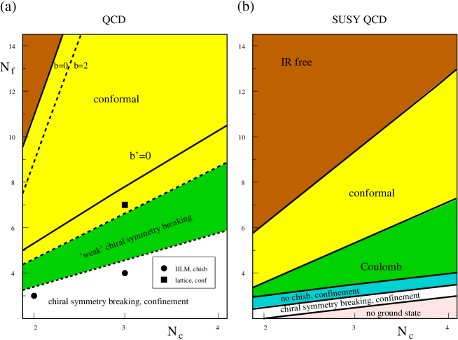
FIG. 42.: Schematic phase diagram of QCD (a) and supersymmetric QCD (b) as a function of the number of colors $N_{c}$ and the number of flavors $N_{f}$.

Naturally, we are mostly interested in the role of instantons in these theories. As $N_{f}$ is increased above the value 2 or 3 (relevant to real QCD) the two basic components of the instanton ensemble, random (individual) instantons and strongly correlated instanton-anti-instanton pairs (molecules) are affected in very different ways. Isolated instantons can only exist if the quark condensate is non-zero, and the instanton density contains the factor $(|\langle\bar{q}q\rangle|\rho^{3})^{N_{f}}$ which comes from the fermion determinant. As a result, small-size instantons are strongly suppressed as $N_{f}$ is increased. This suppression factor does not affect instantons with a size larger than $\rho\sim|\langle\bar{q}q\rangle|^{-1/3}$. This means that as $N_{f}$ is increased, random instantons are pushed to larger sizes. Since in this regime the semi-classical approximation becomes unreliable, we do not know how to calculate the rate of random instantons at large $N_{f}$.

For strongly correlated pairs (molecules) the trend is exactly opposite. The density of pairs is essentially independent of the quark condensate and only determined by the interaction of the two instantons. From purely dimensional considerations one expects the density of molecules to be $dn_{m}\sim d\rho\Lambda^{2b}\rho^{2b-5}$, which means that the typical size becomes smaller as $N_{f}$ is increased [Shu_87b]. If $N_{f}>11N_{c}/2$, we have $b<2$ and the density of pairs is ultraviolet divergent (see the dashed line in Fig. 42(a)). This phenomenon is similar to the UV divergence in the $O(3)$ non-linear $\sigma$ model. Both are examples of UV divergencies of non-perturbative nature. Most likely, they do not have significant effects on the physics of the theory. Since the typical instanton size is small, one would expect that the contribution of molecules at large $N_{f}$ can be reliably calculated. However, since the binding inside the pair increases with $N_{f}$, the separation of perturbative and non-perturbative fluctuations becomes more and more difficult.

Rather than speculate about these effects, let us go back and consider very large $N_{f}$. The solid line labeled $b=0$ in Fig. 42 corresponds to a vanishing first coefficient of the beta function, $b=(11/3)N_{c}-(2/3)N_{f}=0$ in QCD and $b=3N_{c}-N_{f}=0$ in SUSY QCD. Above this line, the coupling constant decreases at large distances, and the theory is IR-free. Below this line, the theory is expected to have an infrared fixed point [BM_74, BZ_82]. As discussed in Sec. III C 3, this is due to the fact that the sign of the the second coefficient of the beta function $b^{\prime}=34N_{c}^{2}/3-13N_{c}N_{f}/3+N_{f}/N_{c}$ is negative while the first one is positive. As a result, the beta function has a zero at $g^{2}_{*}/(16\pi^{2})=-b/b^{\prime}$. This number determines the limiting value of the charge at large distance. Note that the fixed point is not destroyed by higher order perturbative effects, since we can always choose a scheme where higher order coefficients vanish. The presence of an IR fixed point implies that the theory is conformal, that means correlation functions show a power law decay at large distance. There is no mass gap and the long distance behavior is characterized by the set of critical exponents.

Where is the lower boundary of the conformal domain? A recent perturbative study based on the $1/N_{f}$ expansion [Gra_96] suggests that the IR fixed point may persist all the way down to $N_{f}=6$ (for $N_{c}=3$). However, the critical coupling becomes larger and non-perturbative phenomena may become important. For example, [ATW_96] argue that if the coupling constant reaches a critical value the quark-anti-quark interaction is sufficiently strong to break chiral symmetry. In their calculation, this happens for $N_{f}^{c}\simeq 4N_{c}$ (see the dashed line in Fig. 42(a)).

It was then realized that instanton effects can also be important [AS_97]. If the critical coupling is small, even large instantons have a large action $S=8\pi^{2}/g^{2}_{*}\gg 1$ and the semi-classical approximation is valid. As usual, we expect random instantons to contribute to chiral symmetry breaking. According to estimates made in [AS_97], the role of instantons is comparable to perturbative effects in the vicinity of $N_{f}=4N_{c}$. Chiral symmetry breaking is dominated by large instantons with size $\rho\sim|\langle\bar{q}q\rangle|^{-1/3}>\Lambda^{-1}$, while the perturbative regime $\rho<\Lambda^{-1}$ contributes very little. For even larger instantons $\rho\gg|\langle\bar{q}q\rangle|^{-1/3}$ fermions acquire a mass due to chiral symmetry breaking and effectively decouple from gluons. This means that for large distances the charge evolves as in pure gauge theory, and the IR fixed point is only an approximate feature, useful for analyzing the theory above the decoupling scale.

Little is known about the phase structure of multi-flavor QCD from lattice simulations. Lattice QCD with up to 240 flavors was studied in [IKK_96] and it was shown that, as expected, the theory is trivial for $b>0$. The paper also confirms the existence of an infrared fixed point for $N_{f}\geq 7$ ($N_{c}=3$). In Fig. 42(a) we have marked these results by open squares. Other groups have studied QCD with $N_{f}$= 8 [Brown:1992], 12 [Kogut:1988] and 16 [Damgaard:1997] flavors. All of these simulations find a chirally asymmetric and confining theory at strong coupling, and a bulk transition to a chirally symmetric phase (at $\beta=2N_{c}/g^{2}>4.73$, 4.47, 4.12 respectively).

It may appear that these results are in contradiction with the results of Appelquist et al. mentioned above, according to which chiral symmetry should be broken for $N_{f}<12$ ($N_{c}=3$), but this is not the case since the condensate is expected to be exponentially small. In other words, in order to reproduce the subtle mechanism of chiral breaking by large-distance Coulomb exchanges or large-size instantons, the lattice has to include the relevant scales, which is not the case in present lattice simulations.

Present lattice results resemble more closely the results in the interacting instanton liquid discussed in section VII B 4. There we found a line of (rather robust first order) transitions which touches $T=0$ near $N_{f}\simeq 5$. A large drop in the quark condensate in going from $N_{f}=2,3$ to $N_{f}=4$ observed by the Columbia group [CM_97] may very well be the first indication of this phenomenon.

Again, there is no inconsistency between the interacting instanton calculation and the results of Appelquist et al. The IILM calculation takes into account the effects of small instantons only. If small instantons do not break chiral symmetry, then long-range Coulomb forces or large instantons can still be responsible for chiral symmetry breaking. This mechanism was studied by a number of authors, e.g. [aoki, barducci], and the corresponding quark condensate is about an order of magnitude smaller than the one observed for $N_{f}=2$. We would therefore argue that, in a practical sense, QCD has two different phases with chiral symmetry breaking. One, where the quark condensate is large and generated by small size instantons and one where the condensate is significantly smaller and due to Coulomb forces or large instantons. The transition regime is indicated by a wavy line in Fig. 42a. Further studies of the mechanisms of chiral symmetry breaking for different $N_{f}$ are needed before final conclusions can be drawn.

Finally, although experiment tells us that confinement and chiral symmetry breaking go together for $N_{f}=2,3$, the two are independent phenomena and it is conceivable that there are regions in the phase diagram where only one of them takes place. It is commonly believed that confinement implies chiral symmetry breaking, but not even that is entirely clear. In fact, SUSY QCD with $N_{f}=N_{c}+1$ provides a counterexample.

For comparison we also show the phase diagram of ($N=1$) supersymmetric QCD (Fig. 42b). As discussed in section VIII C, the phase structure of these theories was recently clarified by Seiberg and collaborators. In this case, the lower boundary of the conformal domain is at $N_{f}=(3/2)N_{c}$. Below this line the dual theory based on the gauge group $SU(N_{f}-N_{c})$ loses asymptotic freedom. In this case, the excitations are IR free “dual quarks”, or composite light baryons in terms of the original theory. Remarkably, the t’ Hooft matching conditions between the original (short distance) theory and the dual theory based on a completely different gauge group work out exactly. The theory becomes confining for $N_{f}=N_{c}+1$ and $N_{f}=N_{c}$. In the first case chiral symmetry is preserved and the low energy excitations are massless baryons. In the second case, instantons modify the geometry of the space of possible vacua, the point where the excitations are massless baryons is not allowed, and chiral symmetry has to be broken. Note that in ordinary QCD, the ’t Hooft matching conditions cannot be satisfied for a confining phase without chiral symmetry breaking (for $N_{c}\neq 2$). For an even smaller number of flavors, $0<N_{f}\leq N_{c}-1$, massless SUSY QCD does not have a stable ground state. The reason is that instanton-anti-instanton molecules generate a positive vacuum energy density which decreases with the Higgs expectation value, so that the ground state is pushed to infinitely large Higgs VEVs.

We do not shown the phase structure of SUSY QCD with $N>1$ gluinos. In some cases (e.g. $N=4,\,N_{f}=0$ or $N=2,\,N_{f}=4$) the beta function vanishes and the theory is conformal, although instantons may still cause a finite charge renormalization. As already mentioned, the low energy spectrum of the $N=2$ theory was recently determined by Seiberg and Witten. The theory does not have chiral symmetry breaking or confinement, but it contains monopoles/dyons which become massless as the Higgs VEV is decreased. This can be used to trigger confinement when the theory is perturbed to $N=1$.

To summarize, there are many open questions concerning the phase structure of QCD-like theories, and many issues to be explored in future studies, especially on the lattice. The location of the lower boundary of the conformal domain, and the structure of the chirally asymmetric phase in the domain $N_{f}=4-12$ should certainly be studied in more detail. Fascinating results have clarified the rich (and sometimes rather exotic) phase structure of SUSY QCD. To what extent these results will help our understanding of non-supersymmetric theories remains to be seen. In any event, it is certainly clear that instantons and anomalies play a very important, if not dominant, role in both cases.

X Acknowledgments

It is a pleasure to thank our friends and collaborators who have contributed to this review or the work presented here. In particular, we would like to thank our collaborators J. Verbaarschot, M. Velkovsky and A. Blotz. We would like to tank M. Shifman for many valuable comments on the original manuscript. We have also benefitted from discussions with G. E. Brown, D. I. Diakonov, J. Negele, M. Novak, A. V. Smilga, A. Vainshtein and I. Zahed.

XI Notes added in proof

Since this manuscript was prepared, the subject of instantons in QCD has continued to see many interesting developments. We would like to briefly mention some of these, related to instanton searches on the lattice, the relation of instantons with confinement, instantons and charm quarks, instantons at finite chemical potential, and instantons in supersymmetric theories.

Significant progress was made studying topology on the lattice using improved operators, renormalization group techniques, and fermionic methods. Also, first results of studying instantons in the vicinity of the phase transition in full QCD were reported. As an example for the use of improved actions we mention results of Colorado group [DHK_97b] in pure gauge $SU(2)$. They find that chiral symmetry breaking and confinement are preserved by inverse blocking transformation used to smooth the fields. Instantons are easily identified, and inverse blocking (unlike “cooling”) preserves even close instanton-antiinstanton pairs. The instanton size distribution is peaked at $\rho\simeq 0.2$ fm, and large instantons are suppressed.

Low-lying eigenstates of the Dirac operator were studied by the MIT group [IN_97]. They find that the corresponding wave functions are spatially correlated with the locations of instantons, providing support for the picture of the quark condensate as a collective state built from instanton zero modes. In addition to that, they studied the importance of low-lying states in hadronic correlation functions. They demonstrate that the lowest $\sim 100$ modes (out of $\sim 10^{6}$) are sufficient to quantitatively reproduce the hadronic ground state contribution to the $\rho$ and $\pi$ meson correlation functions.

In addition to that, first attempts were made to study instantons at in the vicinity of the finite temperature phase transition in full QCD [FGH_97]. Using the cooling technique to identify instantons, they verified the $T$-dependence of the instanton density discussed in Sect. VII.A. They observe polarized instanton-antiinstanton pairs above $T_{c}$, but these objects do not seem to dominate the ensemble. This point definitely deserves further study, using improved methods and smaller quark masses.

In the main text we stated that there is no confinement in the instanton model. Recently, it was claimed that instantons generate a linear potential with a slope close to the experimental value 1 GeV/fm [Fuk_97]. This prompted [CNS_98] to reinvestigate the issue, and perform high statistics numerical calculations of the heavy-quark potential in the instanton liquid at distances up to 3 fm. The main conclusions are: (i) the potential is larger and significantly longer range than the dilute gas result Equ. (208); (ii) a random ensemble with a realistic size distribution leads to a potential which is linear even for large $R\simeq 3$ fm; (iii) the slope of the potential is still too small, $K\simeq 200$ MeV/fm. This means that the bulk of the confining forces still has to come from some (as of yet?) unidentified objects with small action. These objects may turn out to be large instantons, but that would still imply that the main contribution is not semi-classical. Nevertheless, the result that the heavy quark potential is larger than expected is good news for the instanton model. It implies that even weakly bound states and resonances can be addressed within in the model.

We also did not discuss the role of charm quarks in the QCD vacuum. However, the color field inside a small-size instantons $G_{\mu\nu}\simeq 1\,{\rm GeV}^{2}$ is comparable to the charm quark mass squared $m_{c}^{2}\simeq 2\,{\rm GeV}^{2}$, so one might expect observable effects due to the polarization of charm quark inside ordinary hadrons. Recently, it was suggested that CLEO observations of an unexpectedly large branching ratio $B\rightarrow\eta^{\prime}K$ (as well as inclusive $B\rightarrow\eta^{\prime}+\ldots$) provide a smoking gun for such effects [HZ_98]. The basic idea is that these decays proceed via Cabbibo-unsuppressed $b\to\bar{c}cs$ transition, followed by $\bar{c}c\to\eta^{\prime}$. The charm content of the $\eta^{\prime}$ in the instanton liquid was estimated in [SZ_97], and the result is consistent with what is needed to understand the CLEO data. Another interesting possibility raised in [HZ_97] is that polarized charm quarks give a substantial contribution to the spin $\Sigma$ of the nucleon. A recent instanton calculation only finds a contribution in the range $\Delta c/\Sigma=-(0.08-0.20)$ [BS_97], but the value of $\Delta c$ remains an interesting question for future deep inelastic scattering experiments (e.g. Compass at CERN). In the context of (polarized) nucleon structure functions we should also mention interesting work on leading and non-leading twist operators, see [BPW_97] and references therein.

Finally, Bjorken discussed the possibility that instantons contribute to the decay of mesons containing real $\bar{c}c$ pairs [bj_97]. A particularly interesting case is the $\eta_{c}$, which has three unusual 3-meson decay channels ($\eta^{\prime}\pi\pi$, $\eta\pi\pi$, and $KK\pi$), which contribute roughly 5% each to the total width. This fits well with the typical instanton vertex $\bar{u}u\bar{d}d\bar{s}s$. In general, all of these observables offer the chance to detect non-perturbative effects deep inside the semi-classical domain.

Initial efforts were made to understand the instanton liquid at finite chemical potential [Sch_97]. The suggestion made in this work is that the role that molecules play in the high temperature phase is now played by more complicated “polymers” that are aligned in the time direction. More importantly, it was suggested that instanton lead to the formation of diquark condensates in high density matter [RSS_97, ARW_97]. In the high density phase chiral symmetry is restored, but $SU(3)$ color is broken by a Higgs mechanism.

Instanton effects in SUSY gauge theories continue to be a very active field. For $N=2$ (Seiberg-Witten) theories the $n$-instanton contribution was calculated explicitly [DKM_97, DHK_97], and as a by-product these authors also determined the (classical) $n$-instanton measure in the cases $N=1$ and $N=0$ (non-SUSY). Yung also determined the one-instanton contribution to higher derivative operators beyond the SW effective lagrangian [Yun_97]. Another very interesting result is the generalization of the Seiberg-Witten solution to an arbitrary number of colors $N_{c}$ [DS_95]. This result sheds some light on the puzzling problem of instantons in the large $N_{c}$ limit. The large $N_{c}$ limit is usually performed with $g^{2}N_{c}$ held fixed, and in that case instantons amplitudes are suppressed by $\exp(-N_{c})$. However, [DS_95] found that (at least in the case $N=2$) this is not the correct way to take the large $N_{c}$ limit (if we want to keep the physics unchanged).

A comparison of the running of the effective charge in $N=2,1$ SUSY QCD and QCD was performed in [RRS_98]. In $N=2$ SUSY QCD, the Seiberg-Witten solution shows that instantons accelerate the growth of the coupling. As a result, the coupling blows up at a scale $\Lambda_{NP}>\Lambda_{QCD}$ where the perturbative coupling is still small. A similar phenomenon takes place in QCD if the instanton correction to the running coupling is estimated from the formula of Callan, Dashen, and Gross. This might help to explain why in QCD the non-perturbative scale $\Lambda_{NP}\simeq\Lambda_{\chi SB}\simeq 1\,GeV>\Lambda_{QCD}\simeq 200$ MeV.

A Basic instanton formulas

1 Instanton gauge potential

We use the following conventions for Euclidean gauge fields: The gauge potential is $A_{\mu}=A_{\mu}^{a}\frac{\lambda^{a}}{2}$, where the $SU(N)$ generators satisfy $[\lambda^{a},\lambda^{b}]=2if^{abc}\lambda^{c}$ and are normalized according to ${\rm tr}[\lambda^{a}\lambda^{b}]=2\delta^{ab}$. The covariant derivative is given by $D_{\mu}=\partial_{\mu}-iA_{\mu}$ and the field strength tensor is

$$F_{\mu\nu}=\partial_{\mu}A_{\nu}-\partial_{\nu}A_{\mu}-i[A_{\mu},A_{\nu}].$$ (A1)

In our conventions, the coupling constant is absorbed into the gauge fields. Standard perturbative notation corresponds to the replacement $A_{\mu}\to gA_{\mu}$. The single instanton solution in regular gauge is given by

$$A_{\mu}^{a}=\frac{2\eta_{a\mu\nu}x_{\nu}}{x^{2}+\rho^{2}},$$ (A2)

and the corresponding field strength is

$$G_{\mu\nu}^{a} = -\frac{4\eta_{a\mu\nu}\rho^{2}}{(x^{2}+\rho^{2})^{2}},$$ (A3)

$$(G_{\mu\nu}^{a})^{2} = \frac{192\rho^{4}}{(x^{2}+\rho^{2})^{4}}.$$ (A4)

The gauge potential and field strength in singular gauge are

$$A_{\mu}^{a} = \frac{2\bar{\eta}_{a\mu\nu}x_{\nu}\rho^{2}}{x^{2}(x^{2}+\rho^{2})},$$ (A5)

$$G_{\mu\nu}^{a} = -\frac{4\rho^{2}}{(x^{2}+\rho^{2})^{2}}\left(\bar{\eta}_{a\mu\nu}-2\bar{\eta}_{a\mu\alpha}\frac{x_{\alpha}x_{\nu}}{x^{2}}-2\bar{\eta}_{a\alpha\nu}\frac{x_{\mu}x_{\alpha}}{x^{2}}\right)\;.$$ (A6)

Finally, an $n$-instanton solution in singular gauge is given by

$$A_{\mu}^{a} = \bar{\eta}_{a\mu\nu}\partial_{\nu}\ln\Pi(x),$$ (A7)

$$\Pi(x) = 1+\sum_{i=1}^{n}\frac{\rho_{i}^{2}}{(x-z_{i})^{2}}.$$ (A8)

Note that all instantons have the same color orientation. For a construction that gives the most general $n$-instanton solution, see [AHDM_77].

2 Fermion zero modes and overlap integrals

In singular gauge, the zero mode wave function $iD\!\!\!\!/\,\phi_{0}=0$ is given by

$$\phi_{a\nu}=\frac{1}{2\sqrt{2}\pi\rho}\sqrt{\Pi}\left[\partial\!\!\!/\left(\frac{\Phi}{\Pi}\right)\right]_{\nu\mu}U_{ab}\epsilon_{\mu b},$$ (A9)

where $\Phi=\Pi-1$. For the single instanton solution, we get

$$\phi_{a\nu}(x)=\frac{\rho}{\pi}\frac{1}{(x^{2}+\rho^{2})^{3/2}}\left[\left(\frac{1-\gamma_{5}}{2}\right)\frac{x\!\!\!/}{\sqrt{x^{2}}}\right]_{\nu\mu}U_{ab}\epsilon_{\mu b}.$$ (A10)

The instanton-instanton zero mode density matrices are

$$\phi_{I}(x)_{i\alpha}\phi_{J}^{\dagger}(y)_{j\beta} = \frac{1}{8}\varphi_{I}(x)\varphi_{J}(y)\left(x\!\!\!/\gamma_{\mu}\gamma_{\nu}y\!\!\!/\frac{1-\gamma_{5}}{2}\right)_{ij}\otimes\left(U_{I}\tau_{\mu}^{-}\tau_{\nu}^{+}U_{J}^{\dagger}\right)_{\alpha\beta},$$ (A11)

$$\phi_{I}(x)_{i\alpha}\phi^{\dagger}_{A}(y)_{j\beta} = -\frac{i}{2}\varphi_{I}(x)\varphi_{A}(y)\left(x\!\!\!/\gamma_{\mu}y\!\!\!/\frac{1+\gamma_{5}}{2}\right)_{ij}\otimes\left(U_{I}\tau_{\mu}^{-}U_{A}^{\dagger}\right)_{\alpha\beta},$$ (A12)

$$\phi_{A}(x)_{i\alpha}\phi^{\dagger}_{I}(y)_{j\beta} = \frac{i}{2}\varphi_{A}(x)\varphi_{I}(y)\left(x\!\!\!/\gamma_{\mu}y\!\!\!/\frac{1-\gamma_{5}}{2}\right)_{ij}\otimes\left(U_{A}\tau_{\mu}^{+}U_{I}^{\dagger}\right)_{\alpha\beta},$$ (A13)

with

$$\varphi(x)=\frac{\rho}{\pi}\frac{1}{\sqrt{x^{2}}(x^{2}+\rho^{2})^{3/2}}.$$ (A14)

The overlap matrix element is given by

$$T_{AI} = \int d^{4}x\,\phi_{A}^{\dagger}(x-z_{A})iD\!\!\!\!/\,\phi_{I}(x-z_{I})$$ (A15)

$$= r_{\mu}\,{\rm Tr}(U_{I}\tau_{\mu}^{-}U^{\dagger}_{A})\,\frac{1}{2\pi^{2}r}\frac{d}{dr}M(r),$$ (A16)

with

$$M(r)=\frac{1}{r}\,\int\limits_{0}^{\infty}dp\,p^{2}|\varphi(p)|^{2}J_{1}(pr).$$ (A17)

The fourier transform of zero mode profile is given by

$$\varphi(p)=\pi\rho^{2}\left.\frac{d}{dx}\left(I_{0}(x)K_{0}(x)-I_{1}(x)K_{1}(x)\right)\right|_{x=\frac{p\rho}{2}}.$$ (A18)

3 Properties of $\eta$ symbols

We define 4-vector matrices

$$\tau_{\mu}^{\pm}=(\vec{\tau},\mp i),$$ (A19)

where $\tau^{a}\tau^{b}=\delta^{ab}+i\epsilon^{abc}\tau^{c}$ and

$$\tau_{\mu}^{+}\tau_{\nu}^{-} = \delta_{\mu\nu}+i\eta_{a\mu\nu}\tau^{a},$$ (A20)

$$\tau_{\mu}^{-}\tau_{\nu}^{+} = \delta_{\mu\nu}+i\bar{\eta}_{a\mu\nu}\tau^{a},$$ (A21)

with the $\eta$-symbols given by

$$\eta_{a\mu\nu} = \epsilon_{a\mu\nu}+\delta_{a\mu}\delta_{\nu 4}-\delta_{a\nu}\delta_{\mu 4},$$ (A22)

$$\bar{\eta}_{a\mu\nu} = \epsilon_{a\mu\nu}-\delta_{a\mu}\delta_{\nu 4}+\delta_{a\nu}\delta_{\mu 4}.$$ (A23)

The $\eta$-symbols are (anti) self-dual in the vector indices

$$\eta_{a\mu\nu}=\frac{1}{2}\epsilon_{\mu\nu\alpha\beta}\eta_{a\alpha\beta},\hskip 28.45274pt\bar{\eta}_{a\mu\nu}=-\frac{1}{2}\epsilon_{\mu\nu\alpha\beta}\bar{\eta}_{a\alpha\beta}\hskip 28.45274pt\eta_{a\mu\nu}=-\eta_{a\nu\mu}.$$ (A24)

We have the following useful relations for contractions involving $\eta$ symbols

$$\eta_{a\mu\nu}\eta_{b\mu\nu} = 4\delta_{ab},$$ (A25)

$$\eta_{a\mu\nu}\eta_{a\mu\rho} = 3\delta_{\nu\rho},$$ (A26)

$$\eta_{a\mu\nu}\eta_{a\mu\nu} = 12,$$ (A27)

$$\eta_{a\mu\nu}\eta_{a\rho\lambda} = \delta_{\mu\rho}\delta_{\nu\lambda}-\delta_{\mu\lambda}\delta_{\nu\rho}+\epsilon_{\mu\nu\rho\lambda},$$ (A28)

$$\eta_{a\mu\nu}\eta_{b\mu\rho} = \delta_{ab}\delta_{\nu\rho}+\epsilon_{abc}\eta_{c\nu\rho},$$ (A29)

$$\eta_{a\mu\nu}\bar{\eta}_{b\mu\nu} = 0.$$ (A30)

The same relations hold for $\bar{\eta}_{a\mu\nu}$, except for

$$\bar{\eta}_{a\mu\nu}\bar{\eta}_{a\rho\lambda}=\delta_{\mu\rho}\delta_{\nu\lambda}-\delta_{\mu\lambda}\delta_{\nu\rho}-\epsilon_{\mu\nu\rho\lambda}.$$ (A31)

Some additional relations are

$$\epsilon_{abc}\eta_{b\mu\nu}\eta_{c\rho\lambda} = \delta_{\mu\rho}\eta_{a\nu\lambda}-\delta_{\mu\lambda}\eta_{a\nu\rho}+\delta_{\nu\lambda}\eta_{a\mu\rho}-\delta_{\nu\rho}\eta_{a\mu\lambda},$$ (A32)

$$\epsilon_{\lambda\mu\nu\sigma}\eta_{a\rho\sigma} = \delta_{\rho\lambda}\eta_{a\mu\nu}+\delta_{\rho\nu}\eta_{a\lambda\mu}+\delta_{\rho\mu}\eta_{a\nu\lambda}.$$ (A33)

4 Group integration

In order to perform averages over the color group, we need the following integrands over the invariant $SU(3)$ measure

$$\int dU\,U_{ij}U^{\dagger}_{kl} = \frac{1}{N_{c}}\delta_{jk}\delta_{li},$$ (A34)

$$\int dU\,U_{ij}U^{\dagger}_{kl}U_{mn}U^{\dagger}_{op} = \frac{1}{N_{c}^{2}}\delta_{jk}\delta_{li}\delta_{no}\delta_{mp}+\frac{1}{4(N_{c}^{2}-1)}(\lambda^{a})_{jk}(\lambda^{a})_{li}(\lambda^{b})_{no}(\lambda^{b})_{mp}.$$ (A35)

Additional results can be found in [Cre_83]. These results can be rearranged using $SU(N)$ Fierz transformation

$$(\lambda^{a})_{ij}(\lambda^{a})_{kl} = -\frac{2}{N_{c}}\delta_{ij}\delta_{kl}+2\delta_{jk}\delta_{il}.$$ (A36)

REFERENCES

- [1]
- [2] [] Abbott, L. F., and E. Farhi, 1981, Phys. Lett. B101, 69.
- [3]
- [4] [] Abrikosov, A. A., 1983, Sov. J. Nucl. Phys. 37, 459.
- [5]
- [6] [] Actor, A., 1979, Rev. Mod. Phys. 51, 461.
- [7]
- [8] [] Adami, C., T. Hatsuda, and I. Zahed, 1991, Phys. Rev. D43, 921.
- [9]
- [10] [] Adler, S. L., 1969, Phys. Rev. 177, 2426.
- [11]
- [12] [] Affleck, I., 1981, Nucl. Phys. B191, 429.
- [13]
- [14] [] Affleck, I., M. Dine, and N. Seiberg, 1984a, Phys. Lett. B140, 59.
- [15]
- [16] [] Affleck, I., M. Dine, and N. Seiberg, 1984b, Nucl. Phys. B241, 493.
- [17]
- [18] [] Affleck, I., M. Dine, and N. Seiberg, 1985, Nucl. Phys. B256, 557.
- [19]
- [20] [] Aleinikov, A., and E. Shuryak, 1987, Yad. Fiz. 46, 122.
- [21]
- [22] [] Alfaro, V. D., S. Fubini, and G. Furlan, 1976, Phys. Lett. B65, 163.
- [23]
- [24] [] Alford, M., K. Rajagopal, and F. Wilczek, 1997. hep-ph/9711395.
- [25]
- [26] [] Alles, B., A. DiGiacomo, and M. Gianetti, 1990, Phys. Lett. B249, 490.
- [27]
- [28] [] Alles, B., M. Campostrini, and A. DiGiacomo, 1993, Phys. Rev. D48, 2284.
- [29]
- [30] [] Alles, B., M. D’Elia, and A. DiGiacomo, 1997, Nucl. Phys. B494, 281.
- [31]
- [32] [] Amati, D., K. Konishi, Y. Meurice, G. C. Rossi, and G. Veneziano, 1988, Phys. Rep. 162, 169.
- [33]
- [34] [] Ambjorn, J., and P. Olesen, 1977, Nucl. Phys. B170, 60.
- [35]
- [36] [] Andrei, N., and D. J. Gross, 1978, Phys. Rev. D18, 468.
- [37]
- [38] [] Aoki, K. I., M. Bando, T. Kugo, M. G. Mitchard, and H. Nakatani, 1990, Prog. Theor. Physics 84, 683.
- [39]
- [40] [] Aoyama, H., T. Harano, H. Kikuchi, I. Okouchi, M. Sato, and S. Wada, 1997, Prog. Theor. Phys. Suppl. 127, 1.
- [41]
- [42] [] Aoyama, H., T. Harano, M. Sato, and S. Wada, 1996, Phys. Lett. B388, 331.
- [43]
- [44] [] Appelquist, T., and R. D. Pisarski, 1981, Phys. Rev. D23, 2305.
- [45]
- [46] [] Appelquist, T., and S. B. Selipsky, 1997, Phys. Lett. B 400, 364.
- [47]
- [48] [] Appelquist, T., J. Terning, and L. C. R. Wijewardhana, 1996, Phys. Rev. Lett. 77, 1214.
- [49]
- [50] [] Arnold, P. B., and M. P. Mattis, 1991, Mod. Phys. Lett. A6, 2059.
- [51]
- [52] [] Atiyah, M. F., and N. S. Manton, 1989, Phys. Lett. B222, 438.
- [53]
- [54] [] Atiyah, M. F., N. J. Hitchin, V. G. Drinfeld, and Y. I. Manin, 1977, Phys. Lett. A65, 185.
- [55]
- [56] [] Bagan, E., and S. Steele, 1990, Phys. Lett. B243, 413.
- [57]
- [58] [] Bali, G. S., K. Schilling, A. Hulsebos, A. C. Irving, C. Michael, and P. W. Stephenson, 1993, Phys. Lett. B309, 378.
- [59]
- [60] [] Balitskii, I., and V. Braun, 1995, Phys. Lett. B346, 143.
- [61]
- [62] [] Balitskii, I. I., and V. M. Braun, 1993, Phys. Lett. B314, 237.
- [63]
- [64] [] Balitsky, I. I., and A. Schäfer, 1993, Nucl. Phys. B404, 639.
- [65]
- [66] [] Balitsky, I. I., and A. V. Yung, 1986, Phys. Lett. B168, 113.
- [67]
- [68] [] Balla, J., M. V. Polyakov, and C. Weiss, 1997. hep-ph/9707515.
- [69]
- [70] [] Baluni, V., 1979, Phys. Rev. D19, 2227.
- [71]
- [72] [] Baluni, V., 1981, Phys. Lett. 106B, 491.
- [73]
- [74] [] Banks, T., and A. Casher, 1980, Nucl. Phys. B169, 103.
- [75]
- [76] [] Banks, T., and A. Zaks, 1982, Nucl. Phys. B82, 196.
- [77]
- [78] [] Barducci, A., R. Casalbuoni, S. D. Curtis, D. Dominici, and R. Gatto, 1988, Phys. Rev. D38, 238.
- [79]
- [80] [] Belavin, A. A., A. M. Polyakov, A. A. Schwartz, and Y. S. Tyupkin, 1975, Phys. Lett. B59, 85.
- [81]
- [82] [] Belavin, A. A., and A. A. Migdal, 1974. preprint (Landau Inst.) 74-0894.
- [83]
- [84] [] Bell, J. S., and R. Jackiw, 1969, Nuovo Cimento A60, 47.
- [85]
- [86] [] Belyaev, V. M., and B. L. Ioffe, 1982, Sov. Phys. JETP, 83, 976.
- [87]
- [88] [] Beresinsky, V., 1971, Zhetph 61, 1144.
- [89]
- [90] [] Bernard, C., M. C. Ogilvie, T. A. DeGrand, C. DeTar, S. VGottlieb, A. Krasnitz, R. L. Sugar, and D. Toussaint, 1992, Phys. Rev. Lett. 68, 2125.
- [91]
- [92] [] Bernard, C., T. Blum, C. DeTar, S. Gottlieb, U. M. Heller, J. E. Hetrick, K. Rummukainen, R. Sugar, D. Toussaint, and M. Wingate, 1997, Phys. Rev. Lett. 78, 598.
- [93]
- [94] [] Bernard, C. W., N. H. Christ, A. H. Guth, and E. J. Weinberg, 1977, Phys. Rev. D16, 2967.
- [95]
- [96] [] Bernard, V., and U. G. Meissner, 1988, Phys. Rev. D38, 1551.
- [97]
- [98] [] Bjorken, J. D., 1997. hep-ph/9706524.
- [99]
- [100] [] Blask, W., U. Bohn, M. Huber, B. Metsch, and H. Petry, 1990, Z. Phys. A337, 327.
- [101]
- [102] [] Blotz, A., and E. Shuryak, 1997a, Phys. Rev. D55, 4055.
- [103]
- [104] [] Blotz, A., and E. Shuryak, 1997b. hep-ph/9710544.
- [105]
- [106] [] Blum, T., L. Kärkkäinnen, D. Toussaint, and S. Gottlieb, 1995, Phys. Rev. D51, 5133.
- [107]
- [108] [] Bochkarev, A. I., and M. E. Shaposhnikov, 1986, Nucl. Phys. B268, 220.
- [109]
- [110] [] Bogomolny, E. B., 1980, Phys. Lett. B91, 431.
- [111]
- [112] [] Borgs, C., 1985, Nucl. Phys. B261, 455.
- [113]
- [114] [] Boyd, G., 1996. preprint, hep-lat/9607046.
- [115]
- [116] [] Boyd, G., S. Gupta, F. Karsch, and E. Laerman, 1994, Z. Phys. C64, 331.
- [117]
- [118] [] Brezin, E., G. Parisi, and J. Zinn-Justin., 1977, Phys. Rev. D16, 408.
- [119]
- [120] [] Brower, R. C., K. N. Orginos, and C.-I. Tan, 1997, Phys. Rev. D55, 6313.
- [121]
- [122] [] Brown, F. R., F. P. Butler, H. Chen, N. H. Christ, Z.-H. Dong, W. Schaffer, L. I. Unger, and A. Vaccarino, 1990, Phys. Rev. Lett. 65, 2491.
- [123]
- [124] [] Brown, F. R., et al., 1992, Phys. Rev. D46, 5655.
- [125]
- [126] [] Brown, G. E., and M. Rho, 1978, Comm. Nucl. Part. Phys. 18, 1.
- [127]
- [128] [] Brown, L. S., and D. B. Creamer, 1978, Phys. Rev. D18, 3695.
- [129]
- [130] [] Brown, L. S., R. D. Carlitz, D. B. Creamer, and C. Lee, 1978, Phys. Rev. D17, 1583.
- [131]
- [132] [] Caldi, D., 1977, Phys. Rev. Lett. 39, 121.
- [133]
- [134] [] Callan, C. G., R. Dashen, and D. J. Gross, 1976, Phys. Lett. B63, 334.
- [135]
- [136] [] Callan, C. G., R. Dashen, and D. J. Gross, 1978a, Phys. Rev. D17, 2717.
- [137]
- [138] [] Callan, C. G., R. F. Dashen, and D. J. Gross, 1978b, Phys. Rev. D18, 4684.
- [139]
- [140] [] Callan, C. G., R. F. Dashen, and D. J. Gross, 1979, Phys. Rev. D19, 1826.
- [141]
- [142] [] Campostrini, M., A. DiGiacomo, and H. Panagopoulos, 1988, Phys. Lett. B212, 206.
- [143]
- [144] [] Campostrini, M., A. DiGiacomo, and Y. Gunduc, 1989, Phys. Lett. B225, 393.
- [145]
- [146] [] Carlitz, R. D., and D. B. Creamer, 1979a, Ann. Phys. (NY) 118, 429.
- [147]
- [148] [] Carlitz, R. D., and D. B. Creamer, 1979b, Phys. Lett. B84, 215.
- [149]
- [150] [] Carvalho, C. A. D., 1980, Nucl. Phys. B183, 182.
- [151]
- [152] [] Chandrasekharan, S., 1995, Nucl. Phys. (Proc. Suppl.) B42, 475.
- [153]
- [154] [] Chemtob, M., 1981, Nucl. Phys. B184, 497.
- [155]
- [156] [] Chen, D., and R. D. Mawhinney, 1997, Nucl. Phys. (Proc. Supp.) B53, 216.
- [157]
- [158] [] Chen, D., J. Negele, and E. Shuryak, 1998. The instanton-induced static potential in QCD revisited, MIT preprint.
- [159]
- [160] [] Chernodub, M. N., and F. V. Gubarev, 1995, JETP Lett. 62, 100–104.
- [161]
- [162] [] Chernyshev, S., M. A. Nowak, and I. Zahed, 1996, Phys. Rev. D53, 5176.
- [163]
- [164] [] Christ, N., 1996. talk given at RHIC Summer Study 96, Brookhaven National Laboratory.
- [165]
- [166] [] Christos, G. A., 1984, Phys. Rep. 116, 251.
- [167]
- [168] [] Christov, C. V., A. Blotz, H. Kim, P. Pobylitsa, T. Watabe, T. Meissner, E. Ruiz-Ariola, and K. Goeke, 1996, Prog. Part. Nucl. Phys. 37, 91.
- [169]
- [170] [] Chu, M. C., and S. Schramm, 1995, Phys. Rev. D51, 4580.
- [171]
- [172] [] Chu, M. C., J. M. Grandy, S. Huang, and J. W. Negele, 1993a, Phys. Rev. Lett. 70, 225.
- [173]
- [174] [] Chu, M. C., J. M. Grandy, S. Huang, and J. W. Negele, 1993b, Phys. Rev. D 48, 3340.
- [175]
- [176] [] Chu, M. C., J. M. Grandy, S. Huang, and J. W. Negele, 1994, Phys. Rev. D49, 6039.
- [177]
- [178] [] Chu, M. C., M. Lissia, and J. W. Negele, 1991, Nucl. Phys. B360, 31.
- [179]
- [180] [] Claudson, M., E. Farhi, and R. L. Jaffe, 1986, Phys. Rev. D34, 873.
- [181]
- [182] [] Cohen, E., and C. Gomez, 1984, Phys. Rev. Lett. 52, 237.
- [183]
- [184] [] Coleman, S., 1977, “The uses of instantons”, Proc. of the 1977 School of Subnuclear Physics, Erice (Italy), reproduced in Aspects of Symmetry, Cambridge University Press (1985), page 265.
- [185]
- [186] [] Cooper, F., A. Khare, and U. Sukhatme, 1995, Phys. Rep. 251, 267.
- [187]
- [188] [] Corrigan, E., P. Goddard, and S. Templeton, 1979, Nucl. Phys. B151, 93.
- [189]
- [190] [] Creutz, M., 1983, Quarks, gluons and lattices (Cambridge University Press, Cambridge).
- [191]
- [192] [] Crewther, R. J., P. D. Vecchia, G. Veneziano, and E. Witten, 1979, Phys. Lett. B88, 123.
- [193]
- [194] [] Damgaard, P. H., U. M. Heller, A. Krasnitz, and P. Olesen, 1997, Phys. Lett. B 400, 169.
- [195]
- [196] [] de Forcrand, F., and K.-F. Liu, 1992, Phys. Rev. Lett. 69, 245.
- [197]
- [198] [] de Forcrand, P., M. G. Perez, and I.-O. Stamatescu, 1996, Nucl. Phys. Proc. Suppl. 47, 777.
- [199]
- [200] [] de Forcrand, P., M. G. Perez, and I.-O. Stamatescu, 1997, Nucl. Phys. B 499, 409.
- [201]
- [202] [] de Forcrand, P., M. G. Perez, J. E. Hetrick, and I.-O. Stamatescu, 1997. hep-lat/9802017.
- [203]
- [204] [] DeGrand, T., A. Hasenfratz, and T. G. Kovacs, 1997. hep-lat/9710078.
- [205]
- [206] [] DeGrand, T., R. Jaffe, K. Johnson, and J. Kiskis, 1975, Phys. Rev. D12, 2060.
- [207]
- [208] [] DelDebbio, L., M. Faber, J. Greensite, and S. Olejnik, 1997, Nucl. Phys. Proc. Suppl. 53, 141.
- [209]
- [210] [] Deng, Y., 1989, Nucl. Phys. (Proc. Suppl.) B9, 334.
- [211]
- [212] [] Dey, M., V. L. Eletsky, and B. L. Ioffe, 1990, Phys. Lett. B252, 620.
- [213]
- [214] [] Diakonov, D. I., 1995. International School of Physics, Enrico Fermi, Course 80, Varenna, Italy.
- [215]
- [216] [] Diakonov, D. I., 1996, Prog. Part. Nucl. Phys. 36, 1.
- [217]
- [218] [] Diakonov, D. I., and A. D. Mirlin, 1988, Phys. Lett. B203, 299.
- [219]
- [220] [] Diakonov, D. I., and M. Polyakov, 1993, Nucl. Phys. B389, 109.
- [221]
- [222] [] Diakonov, D. I., and V. Y. Petrov, 1984, Nucl. Phys. B245, 259.
- [223]
- [224] [] Diakonov, D. I., and V. Y. Petrov, 1985, Sov. Phys. JETP 62, 204.
- [225]
- [226] [] Diakonov, D. I., and V. Y. Petrov, 1986, Nucl. Phys. B272, 457.
- [227]
- [228] [] Diakonov, D. I., and V. Y. Petrov, 1994, Phys. Rev. D50, 266.
- [229]
- [230] [] Diakonov, D. I., and V. Y. Petrov, 1996. Proceedings of the Workshop on Continous advances in QCD, World Scientific, Singapore.
- [231]
- [232] [] Diakonov, D. I., V. Y. Petrov, and P. V. Pobylitsa, 1988, Nucl. Phys. B306, 809.
- [233]
- [234] [] Diakonov, D., V. Petrov, and P. Pobylitsa, 1989, Phys. Lett. B226, 372.
- [235]
- [236] [] Dine, M., and W. Fischler, 1983, Phys. Lett. B120, 137.
- [237]
- [238] [] Dorey, N., T. J. Hollowood, V. V. Khoze, and M. P. Mattis, 1997. hep-th/9709072.
- [239]
- [240] [] Dorey, N., V. Khoze, and M. Mattis, 1996a, Phys. Rev. D54, 2921.
- [241]
- [242] [] Dorey, N., V. Khoze, and M. Mattis, 1996b, Phys. Rev. D 54, 7832.
- [243]
- [244] [] Dorey, N., V. V. Khoze, and M. P. Mattis, 1997. hep-th/9708036.
- [245]
- [246] [] Dorokhov, A. E., and N. I. Kochelev, 1990, Z. Phys. C 46, 281.
- [247]
- [248] [] Dorokhov, A. E., and N. I. Kochelev, 1993, Phys. Lett. B304, 167.
- [249]
- [250] [] Dorokhov, A. E., N. I. Kochelev, and Y. A. Zubov, 1993, Int. J. Mod. Phys. A8, 603.
- [251]
- [252] [] Dorokhov, A. E., Y. A. Zubov, and N. I. Kochelev, 1992, Sov. J. Part. Nuc. 23, 522.
- [253]
- [254] [] Douglas, M. R., and S. H. Shenker, 1995, Nucl. Phys. B447, 271–296.
- [255]
- [256] [] Dowrick, N., and N. McDougall, 1993, Nucl. Phys. B399, 426.
- [257]
- [258] [] Dubovikov, M. S., and A. V. Smilga, 1981, Nucl. Phys. B185, 109.
- [259]
- [260] [] Eguchi, T., P. B. Gilkey, and A. J. Hanson, 1980, Phys. Rept. 66, 213.
- [261]
- [262] [] Eletskii, V. L., and B. L. Ioffe, 1993, Phys. Rev. D47, 3083.
- [263]
- [264] [] Eletsky, V. L., 1993, Phys. Lett. B299, 111.
- [265]
- [266] [] Eletsky, V. L., and B. L. Ioffe, 1988, Sov. J. Nucl. Phys. 48, 384.
- [267]
- [268] [] Espinosa, O., 1990, Nucl. Phys. B343, 310.
- [269]
- [270] [] Evans, N., S. D. H. Hsu, and M. Schwetz, 1996, Phys. Lett. B375, 262.
- [271]
- [272] [] Faber, M., H. Markum, S. Olejnik, and W. Sakuler, 1995, Nucl. Phys. (Proc.Suppl.) B42, 487.
- [273]
- [274] [] Faleev, S. V., and P. G. Silvestrov, 1995, Phys. Lett. A197, 372.
- [275]
- [276] [] Feurstein, M., H. Markum, and S. Thurner, 1997, Phys. Lett. B 396, 203.
- [277]
- [278] [] Feynman, R. P., and A. R. Hibbs, 1965, Quantum mechanics and path integrals (Mc Graw-Hill, New York).
- [279]
- [280] [] Finnel, D., and P. Pouliot, 1995, Nucl. Phys. B453, 225.
- [281]
- [282] [] Forkel, H., and M. K. Banerjee, 1993, Phys. Rev. Lett. 71, 484.
- [283]
- [284] [] Forkel, H., and M. Nielsen, 1995, Phys. Lett. B345, 55.
- [285]
- [286] [] Förster, D., 1977, Phys. Lett. B66, 279.
- [287]
- [288] [] Forte, S., and E. V. Shuryak, 1991, Nucl. Phys. B357, 153.
- [289]
- [290] [] Fox, I. A., J. P. Gilchrist, M. L. Laursen, and G. Schierholz, 1985, Phys. Rev. Lett. 54, 749.
- [291]
- [292] [] Fried, D., and K. Uhlenbeck, 1984, Instantons and Four-Manifolds (Sringer, New York).
- [293]
- [294] [] Fukushima, M., H. Suganuma, A. Tanaka, H. Toki, and S. Sasaki, 1997. hep-lat/9709133.
- [295]
- [296] [] Georgi, H., and A. Manohar, 1984, Nucl. Phys. B234, 189.
- [297]
- [298] [] Gerber, P., and H. Leutwyler, 1989, Nucl. Phys. B321, 387.
- [299]
- [300] [] Geshkenbein, B., and B. Ioffe, 1980, B166 Nucl. Phys., 340.
- [301]
- [302] [] Gocksch, A., 1991, Phys. Rev. Lett. 67, 1701.
- [303]
- [304] [] Gonzalez-Arroyo, A., and A.Montero, 1996, Phys. Lett. B387, 823.
- [305]
- [306] [] Gracey, J. A., 1996, Phys. Lett. B373, 178.
- [307]
- [308] [] Grandy, J., and R. Gupta, 1994, Nucl. Phys. B(Proc. Suppl.) 34, 164.
- [309]
- [310] [] Gribov, V. N., 1981. preprint, KFKI-1981-66, Budapest.
- [311]
- [312] [] Gross, D. J., R. D. Pisarski, and L. G. Yaffe, 1981, Rev. Mod. Phys. 53, 43.
- [313]
- [314] [] Grossman, B., 1977, Phys. Lett. A61, 86.
- [315]
- [316] [] Gupta, R., 1992. Scaling, the renormalization group and improved lattice actions, LA-UR-92-917, Los Alamos.
- [317]
- [318] [] Gupta, R., D. Daniel, and J. Grandy, 1993, Phys. Rev. D48, 3330.
- [319]
- [320] [] Halperin, I., and A. Zhitnitsky, 1997. hep-ph/9706251.
- [321]
- [322] [] Halperin, I., and A. Zhitnitsky, 1998, Phys. Rev. Lett. 80, 438.
- [323]
- [324] [] Hansson, T. H., and I. Zahed, 1992, Nucl. Phys. B374, 277.
- [325]
- [326] [] Hansson, T. H., M. Sporre, and I. Zahed, 1994, Nucl. Phys. B427, 545.
- [327]
- [328] [] Harrington, B. J., and H. K. Shepard, 1978, Phys. Rev. D17, 2122.
- [329]
- [330] [] Hart, A., and M. Teper, 1995, Phys. Lett. B371, 261.
- [331]
- [332] [] Hasenfratz, A., T. DeGrand, and D. Zhu, 1996, Nucl. Phys. B478, 349.
- [333]
- [334] [] Hatsuda, T., and T. Kunihiro, 1985, Prog. Theor. Phys. 74, 765.
- [335]
- [336] [] Hatsuda, T., and T. Kunihiro, 1994, Phys. Rep. 247, 221.
- [337]
- [338] [] Hatsuda, T., Y. Koike, and S. H. Lee, 1993, Nucl. Phys. B394, 221.
- [339]
- [340] [] Hecht, M., and T. DeGrand, 1992, Phys. Rev. D46, 2115.
- [341]
- [342] [] Hoek, J., 1986, Phys. Lett. B166, 199.
- [343]
- [344] [] Hoek, J., M. Teper, and J. Waterhouse, 1987, Nucl. Phys. B288, 589.
- [345]
- [346] [] Huang, Z., and X.-N. Wang, 1996, Phys. Rev. D53, 5034.
- [347]
- [348] [] Hutter, M., 1997, Z. Phys. C 74, 131.
- [349]
- [350] [] Ilgenfritz, E., and M. Müller-Preussker, 1981, Nucl. Phys. B184, 443.
- [351]
- [352] [] Ilgenfritz, E.-M., and E. V. Shuryak, 1989, Nucl. Phys. B319, 511.
- [353]
- [354] [] Ilgenfritz, E.-M., and E. V. Shuryak, 1994, Phys. Lett. B325, 263.
- [355]
- [356] [] Ilgenfritz, E.-M., M. Müller-Preußker, and E. Meggiolaro, 1995, Nucl. Phys. (Proc. Suppl.) B42, 496.
- [357]
- [358] [] Intriligator, K., and N. Seiberg, 1996, Nucl. Phys. Proc. Suppl. 45BC, 1.
- [359]
- [360] [] Ioffe, B. L., 1981, Nucl. Phys., B188, 317.
- [361]
- [362] [] Irback, A., P. LaCock, D. Miller, B. Peterson, and T. Reisz, 1991, Nucl. Phys. B363, 34.
- [363]
- [364] [] Ishikawa, K., G. Schierholz, H. Schneider, and M. Teper, 1983, Phys. Lett. B128, 309.
- [365]
- [366] [] Ito, K., and N. Sasakura, 1996, Phys. Lett. B382, 95.
- [367]
- [368] [] Ivanenko, T. L., and J. W. Negele, 1997. hep-lat/9709130.
- [369]
- [370] [] Iwasaki, Y., K. Kanaya, S. Kaya, S. Sakai, and T. Yoshie, 1996, Z. Phys. C71, 343.
- [371]
- [372] [] Iwasaki, Y., K. Kanaya, S. Sakai, and T. Yoshie, 1991, Phys. Rev. Lett. 67, 1491.
- [373]
- [374] [] Jack, I., D. R. T. Jones, and C. G. North, 1997, Nucl. Phys. B486, 479.
- [375]
- [376] [] Jackiw, R., and C. Rebbi, 1976a, Phys. Rev. Lett. 37, 172.
- [377]
- [378] [] Jackiw, R., and C. Rebbi, 1976b, Phys. Rev. D14, 517.
- [379]
- [380] [] Jackiw, R., and C. Rebbi, 1977, Phys. Rev. D16, 1052.
- [381]
- [382] [] Jackiw, R., C. Nohl, and C. Rebbi, 1977, Phys. Rev. D15, 1642.
- [383]
- [384] [] Jackson, A. D., and J. J. M. Verbaarschot, 1996, Phys. Rev. D53, 7223.
- [385]
- [386] [] Ji, X., 1995, Phys. Rev. Lett. 74, 1071.
- [387]
- [388] [] Kacir, M., M. Prakash, and I. Zahed, 1996. preprint, hep-ph/9602314.
- [389]
- [390] [] Kanki, T., 1988. Proceedings of the International Workshop on Variational Calculations in Quantum Field Theory, L. Polley, D. Pottinger, (Eds.), World Scientific, Singapore, page 215.
- [391]
- [392] [] Kaplan, D. B., 1992, Phys. Lett. B288, 342.
- [393]
- [394] [] Kapusta, J., 1989, Finite tempearture field theory (Cambridge University Press, Cambridge).
- [395]
- [396] [] Kapusta, J., D. Kharzeev, and L. McLerran, 1996, Phys. Rev. D53, 5028.
- [397]
- [398] [] Karsch, F., and E. Laermann, 1994, Phys. Rev. D50, 6954.
- [399]
- [400] [] Khoze, V., and A. Yung, 1991, Z. Phys. C50, 155.
- [401]
- [402] [] Kikuchi, H., and J. Wudka, 1992, Phys. Lett. B284, 111.
- [403]
- [404] [] Kim, J. E., 1979, Phys. Rev. Lett. 43, 103.
- [405]
- [406] [] Kirkwood, J. G., 1931, J. Chem. Phys. 22, 1420.
- [407]
- [408] [] Klevansky, S. P., 1992, Rev. Mod. Phys. 64, 649.
- [409]
- [410] [] Klimt, S., M. Lutz, and W. Weise, 1990, Phys. Lett. B249, 386.
- [411]
- [412] [] Klinkhammer, F. R., and N. S. Manton, 1984, Phys. Rev. D30, 2212.
- [413]
- [414] [] Koch, V., and G. E. Brown, 1993, Nucl. Phys. A560, 345.
- [415]
- [416] [] Koch, V., E. V. Shuryak, G. E. Brown, and A. D. Jackson, 1992, Phys. Rev. D46, 3169.
- [417]
- [418] [] Koesterlitz, J. M., and D. J. Thouless, 1973, J. Phys. C6, 118.
- [419]
- [420] [] Kogan, I. I., and M. Shifman, 1995, Phys. Rev. Lett. 75, 2085.
- [421]
- [422] [] Kogut, J. B., 1979, Rev. Mod. Phys. 51, 659.
- [423]
- [424] [] Kogut, J. B., and D. K. Sinclair, 1988, Nucl. Phys. B295, 465.
- [425]
- [426] [] Kovner, A., and M. Shifman, 1997, Phys. Rev. D 56, 2396.
- [427]
- [428] [] Kronfeld, A., G. Schierholz, and U. J. Wiese, 1987, Nucl. Phys. B293, 461.
- [429]
- [430] [] Kronfeld, A. S., 1988, Nucl. Phys. (Proc. Supp.) B4, 329.
- [431]
- [432] [] Kuzmin, V. A., V. A. Rubakov, and M. E. Shaposhnikov, 1985, Phys. Lett. B155, 36.
- [433]
- [434] [] Landau, L. D., and E. M. Lifshitz, 1959, Quantum Mechanics (Pergamon Press, Oxford).
- [435]
- [436] [] Laursen, M., J. Smit, and J. C. Vink, 1990, Nucl. Phys. B343, 522.
- [437]
- [438] [] Lee, C., and W. A. Bardeen, 1979, Nucl. Phys. B153, 210.
- [439]
- [440] [] Lee, S. H., and T. Hatsuda, 1996, Phys. Rev. D54, 1871.
- [441]
- [442] [] Leinweber, D. B., 1995a, Phys. Rev. D 51, 6369.
- [443]
- [444] [] Leinweber, D. B., 1995b, Phys. Rev. D 51, 6383.
- [445]
- [446] [] Levine, H., and L. G. Yaffe, 1979, Phys. Rev. D19, 1225.
- [447]
- [448] [] Lipatov, L. N., 1977, JETP Lett. 22, 104.
- [449]
- [450] [] Luescher, M., 1982, Comm. Math. Phys 85, 39.
- [451]
- [452] [] Maggiore, M., and M. Shifman, 1992a, Phys. Rev. D46, 3550.
- [453]
- [454] [] Maggiore, M., and M. Shifman, 1992b, Nucl. Phys. B371, 177.
- [455]
- [456] [] Mandelstam, S., 1976, Phys. Rep. 23, 245.
- [457]
- [458] [] Manousakis, E., and J. Polonyi, 1987, Phys. Rev. Lett. 58, 847.
- [459]
- [460] [] McLerran, L., 1986, Rev. Mod. Phys. 58, 1021.
- [461]
- [462] [] Mermin, N., and H. Wagner, 1966, Phys. Rev. Lett. 16, 1133.
- [463]
- [464] [] Michael, C., and P. S. Spencer, 1994, Phys. Rev. D50, 7570.
- [465]
- [466] [] Michael, C., and P. S. Spencer, 1995, Phys. Rev. D52, 4691.
- [467]
- [468] [] Montvay, I., and G. Münster, 1995, Quantum fields on a lattice (Oxford University Press, Oxford).
- [469]
- [470] [] Münster, G., 1982, Zeit. Phys. C12, 43.
- [471]
- [472] [] Nambu, Y., and G. Jona-Lasinio, 1961, Phys. Rev. 122, 345.
- [473]
- [474] [] Narayanan, R., and H. Neuberger, 1995, Nucl. Phys. B443, 305.
- [475]
- [476] [] Narayanan, R., and P. Vranas, 1997, Nucl. Phys. B 506, 373.
- [477]
- [478] [] Narison, S., 1984, Z. Phys. C26, 209.
- [479]
- [480] [] Narison, S., 1989, QCD spectral sum rules (World Scientific, Singapore).
- [481]
- [482] [] Narison, S., 1996, Phys. Lett. B387, 162.
- [483]
- [484] [] Novak, M., G. Papp, and I. Zahed, 1996, Phys. Lett. B389, 341.
- [485]
- [486] [] Novikov, V. A., 1987, Sov. J. Nucl. Phys. 46, 366.
- [487]
- [488] [] Novikov, V. A., M. A. Shifman, A. I. Vainshtein, and V. I. Zakharov, 1979, Nucl. Phys. B165, 67.
- [489]
- [490] [] Novikov, V. A., M. A. Shifman, A. I. Vainshtein, and V. I. Zakharov, 1980, Nucl. Phys. B165, 55.
- [491]
- [492] [] Novikov, V. A., M. A. Shifman, A. I. Vainshtein, and V. I. Zakharov, 1981, Nucl. Phys. B191, 301.
- [493]
- [494] [] Novikov, V. A., M. A. Shifman, A. I. Vainshtein, and V. I. Zakharov, 1983, Nucl. Phys. B229, 381.
- [495]
- [496] [] Novikov, V. A., M. A. Shifman, A. I. Vainshtein, and V. I. Zakharov, 1985a, Nucl. Phys. B260, 157.
- [497]
- [498] [] Novikov, V. A., M. A. Shifman, A. I. Vainshtein, and V. I. Zakharov, 1985b, Fortschr. Phys. 32, 585.
- [499]
- [500] [] Novikov, V. A., M. A. Shifman, V. B. Voloshin, and V. I. Zakharov, 1983, Nucl. Phys. B229, 394.
- [501]
- [502] [] Nowak, M., 1991, Acta Phys. Pol. B22, 697.
- [503]
- [504] [] Nowak, M. A., J. J. M. Verbaarschot, and I. Zahed, 1989a, Nucl. Phys. B324, 1.
- [505]
- [506] [] Nowak, M. A., J. J. M. Verbaarschot, and I. Zahed, 1989b, Phys. Lett. B228, 115.
- [507]
- [508] [] Nowak, M. A., J. J. M. Verbaarschot, and I. Zahed, 1989c, Nucl. Phys. B325, 581.
- [509]
- [510] [] Olejnik, S., 1989, Phys. Lett. B221, 372.
- [511]
- [512] [] Peccei, R., and H. R. Quinn, 1977, Phys. Rev. D16, 1791.
- [513]
- [514] [] Phillips, A., and D. Stone, 1986, Comm. Math. Phys 103, 599.
- [515]
- [516] [] Pisarski, R. D., and F. Wilczek, 1984, Phys. Rev. D29, 338.
- [517]
- [518] [] Pisarski, R. D., and L. G. Yaffe, 1980, Phys. Lett. B97, 110.
- [519]
- [520] [] Pisarski, R. D., and M. Tytgat, 1997. preprint, hep-ph/9702340.
- [521]
- [522] [] Pobylitsa, P., 1989, Phys. Lett. B226, 387.
- [523]
- [524] [] Polikarpov, M. I., and A. I. Veselov, 1988, Nucl. Phys. B297, 34.
- [525]
- [526] [] Polyakov, A., 1977, Nucl. Phys. B120, 429.
- [527]
- [528] [] Polyakov, A., 1987, Gauge Fields and Strings (Harwood, Chur, Switzerland).
- [529]
- [530] [] Polyakov, A. M., 1975, Phys. Lett. B59, 79.
- [531]
- [532] [] Polyakov, A. M., 1978, Phys. Lett. B72, 477.
- [533]
- [534] [] Preskill, J., M. B. Wise, and F. Wilczek, 1983, Phys. Lett. B120, 133.
- [535]
- [536] [] Pugh, D. J. R., and M. Teper, 1989, Phys. Lett. B224, 159.
- [537]
- [538] [] Rajagopal, K., and F. Wilczek, 1993, Nucl. Phys. B399, 395.
- [539]
- [540] [] Rajaraman, R., 1982, Solitons and Instantons (North Holland, Amsterdam).
- [541]
- [542] [] Randall, L., R. Rattazzi, and E. Shuryak, 1998. hep-ph/9803258.
- [543]
- [544] [] Rapp, R., T. Schäfer, E. V. Shuryak, and M. Velkovsky, 1997. hep-ph/9711396.
- [545]
- [546] [] Reinders, L. J., H. Rubinstein, and S. Yazaki, 1985, Phys. Rep. 127, 1.
- [547]
- [548] [] Ringwald, A., 1990, Nucl. Phys. B330, 1.
- [549]
- [550] [] Ringwald, A., and F. Schrempp, 1994. Proceedings of the International Seminar Quarks 94, Vladimir, Russia, preprint, hep-ph/9411217.
- [551]
- [552] [] Rothe, H. J., 1992, Lattice gauge theories, an introduction (World Scientific, Singapore).
- [553]
- [554] [] S. Caracciolo, R. Edwards, A. P., and A. D. Sokal, 1995, Phys. Rev. Lett. 75, 1891.
- [555]
- [556] [] Salomonson, P., and J. W. V. Holton, 1981, Nucl. Phys. B196, 509.
- [557]
- [558] [] Savvidy, G. K., 1977, Phys. Lett. B71, 133.
- [559]
- [560] [] Schäfer, T., 1996, Phys. Lett. B389, 445.
- [561]
- [562] [] Schäfer, T., 1997. hep-ph/9708256.
- [563]
- [564] [] Schäfer, T., and E. V. Shuryak, 1995a, Phys. Rev. Lett. 75, 1707.
- [565]
- [566] [] Schäfer, T., and E. V. Shuryak, 1995b, Phys. Lett. B356, 147.
- [567]
- [568] [] Schäfer, T., and E. V. Shuryak, 1996a, Phys. Rev D53, 6522.
- [569]
- [570] [] Schäfer, T., and E. V. Shuryak, 1996b, Phys. Rev. D54, 1099.
- [571]
- [572] [] Schäfer, T., E. V. Shuryak, and J. J. M. Verbaarschot, 1994, Nucl. Phys. B412, 143.
- [573]
- [574] [] Schäfer, T., E. V. Shuryak, and J. J. M. Verbaarschot, 1995, Phys. Rev. D51, 1267.
- [575]
- [576] [] Schierholz, G., 1994, Nucl. Phys. Proc. Suppl. 37A, 203.
- [577]
- [578] [] Schramm, S., and M. C. Chu, 1993, Phys. Rev. D48, 2279.
- [579]
- [580] [] Schwarz, A. S., 1977, Phys. Lett. B67, 172.
- [581]
- [582] [] Seiberg, N., 1994, Phys. Rev. D49, 6857.
- [583]
- [584] [] Seiberg, N., and E. Witten, 1994, Nucl. Phys. B426, 19.
- [585]
- [586] [] Shifman, M., 1994, Instantons in Gauge Theories (World Scientific, Singapore).
- [587]
- [588] [] Shifman, M. A., 1989, Sov. Phys. Usp. 32, 289.
- [589]
- [590] [] Shifman, M. A., 1992, Vacuum Structure and QCD Sum Rules (North Holland, Amsterdam).
- [591]
- [592] [] Shifman, M. A., A. I. Vainshtein, and V. I. Zakharov, 1979, Nucl. Phys. B147, 385, 448.
- [593]
- [594] [] Shifman, M. A., A. I. Vainshtein, and V. I. Zakharov, 1980a, Nucl. Phys. B166, 493.
- [595]
- [596] [] Shifman, M. A., A. I. Vaishtein, and V. I. Zakharov, 1978, Phys. Lett. B76, 971.
- [597]
- [598] [] Shifman, M. A., and A. I. Vainshtein, 1988, Nucl. Phys. B296, 445.
- [599]
- [600] [] Shifman, M., A. Vainshtein, and V. Zakharov, 1980b, Nucl. Phys. B165, 45.
- [601]
- [602] [] Shifman, M., A. Vainshtein, and V. Zakharov, 1980c, Nucl. Phys. B163, 46.
- [603]
- [604] [] Shuryak, E., 1978a, Zh. Eksp. Teor. Fiz. (Sov. Phys. JETP), 74, 408.
- [605]
- [606] [] Shuryak, E., 1980, Phys. Rep. 61, 71.
- [607]
- [608] [] Shuryak, E., and M. Velkovsky, 1997. preprint, hep-ph/9703345.
- [609]
- [610] [] Shuryak, E. V., 1978b, Phys. Lett. B79, 135.
- [611]
- [612] [] Shuryak, E. V., 1981, Phys. Lett. B107, 103.
- [613]
- [614] [] Shuryak, E. V., 1982a, Nucl. Phys., B198, 83.
- [615]
- [616] [] Shuryak, E. V., 1982b, Nucl. Phys. B203, 93.
- [617]
- [618] [] Shuryak, E. V., 1982c, Nucl. Phys. B203, 116.
- [619]
- [620] [] Shuryak, E. V., 1982d, Nucl. Phys. B203, 140.
- [621]
- [622] [] Shuryak, E. V., 1983, Nucl. Phys. B214, 237.
- [623]
- [624] [] Shuryak, E. V., 1985, Phys. Lett. B153, 162.
- [625]
- [626] [] Shuryak, E. V., 1987, Phys. Lett. B196, 373.
- [627]
- [628] [] Shuryak, E. V., 1988a, Nucl. Phys. B302, 559, 574, 599.
- [629]
- [630] [] Shuryak, E. V., 1988b, Nucl. Phys. B302, 621.
- [631]
- [632] [] Shuryak, E. V., 1988c, The QCD Vacuum, Hadrons and the Superdense Matter (World Scientific, Singapore).
- [633]
- [634] [] Shuryak, E. V., 1989, Nucl. Phys. B319, 521, 541.
- [635]
- [636] [] Shuryak, E. V., 1993, Rev. Mod. Phys. 65, 1.
- [637]
- [638] [] Shuryak, E. V., 1994, Comm. Nucl. Part. Phys. 21, 235.
- [639]
- [640] [] Shuryak, E. V., 1995, Phys. Rev. D52, 5370.
- [641]
- [642] [] Shuryak, E. V., and A. R. Zhitnitsky, 1997. hep-ph/9706316.
- [643]
- [644] [] Shuryak, E. V., and J. J. M. Verbaarschot, 1990, Nucl. Phys. B341, 1.
- [645]
- [646] [] Shuryak, E. V., and J. J. M. Verbaarschot, 1991, Nucl. Phys. B364, 255.
- [647]
- [648] [] Shuryak, E. V., and J. J. M. Verbaarschot, 1992, Phys. Rev. Lett. 68, 2576.
- [649]
- [650] [] Shuryak, E. V., and J. J. M. Verbaarschot, 1993a, Nucl. Phys. B410, 55.
- [651]
- [652] [] Shuryak, E. V., and J. J. M. Verbaarschot, 1993b, Nucl. Phys. B410, 37.
- [653]
- [654] [] Shuryak, E. V., and J. J. M. Verbaarschot, 1995, Phys. Rev. D52, 295.
- [655]
- [656] [] Shuryak, E. V., and J. L. Rosner, 1989, Phys. Lett. B218, 72.
- [657]
- [658] [] Shuryak, E. V., and M. Velkovsky, 1994, Phys. Rev. D50, 3323.
- [659]
- [660] [] Skyrme, T., 1961, Proc. R. Soc. (London) A262, 207.
- [661]
- [662] [] Smilga, A., 1994a, Phys. Rev. D49, 5480.
- [663]
- [664] [] Smilga, A., 1994b, Phys. Rev. D49, 6836.
- [665]
- [666] [] Smilga, A., and J. Stern, 1993, Phys. Lett. B318, 531.
- [667]
- [668] [] Smilga, A. V., 1997, Phys. Rep. 291, 1.
- [669]
- [670] [] Smit, J., and A. J. van der Sijs, 1989, Nucl. Phys. B355, 603.
- [671]
- [672] [] Smit, J., and J. C. Vink, 1987, Nucl. Phys. B284, 234.
- [673]
- [674] [] Smit, J., and J. C. Vink, 1988, Nucl. Phys. B298, 557.
- [675]
- [676] [] Snyderman, N., and S. Gupta, 1981, Phys. Rev. D24, 542.
- [677]
- [678] [] Steele, J., A. Subramanian, and I. Zahed, 1995, Nucl. Phys. B452, 545.
- [679]
- [680] [] Suganuma, H., A. Tanaka, S. Sasaki, and O. Miyamura, 1996, Nucl. Phys. Proc. Suppl. 47, 302.
- [681]
- [682] [] Suzuki, T., 1993, Nucl. Phys. (Proc. Supp.) B30, 176.
- [683]
- [684] [] Svetitsky, B., and L. G. Yaffe, 1982, Nucl. Phys. B210, 423.
- [685]
- [686] [] ’t Hooft, G., 1976a, Phys. Rev. Lett. 37, 8.
- [687]
- [688] [] ’t Hooft, G., 1976b, Phys. Rev. D14, 3432.
- [689]
- [690] [] ’t Hooft, G., 1981a, Comm. Math. Phys. 81, 267.
- [691]
- [692] [] ’t Hooft, G., 1981b, Nucl. Phys. B190, 455.
- [693]
- [694] [] ’t Hooft, G., 1986, Phys. Rep. 142, 357.
- [695]
- [696] [] Takeuchi, S., and M. Oka, 1991, Phys. Rev. Lett. 66, 1271.
- [697]
- [698] [] Tar, C. D., and J. Kogut, 1987, Phys. Rev. D36, 2828.
- [699]
- [700] [] Teper, M., 1986, Phys. Lett. B171, 86.
- [701]
- [702] [] Thomas, A. W., S. Theberge, and G. A. Miller, 1981, Phys. Rev. D24, 216.
- [703]
- [704] [] Thurner, S., M. Feurstein, and H. Markum, 1997, Phys. Rev. D 56, 4039.
- [705]
- [706] [] Ukawa, A., 1997, Nucl. Phys. Proc. Suppl. 53, 106.
- [707]
- [708] [] Vafa, C., and E. Witten, 1984, Nucl. Phys. B234, 173.
- [709]
- [710] [] Vainshtein, A. I., M. A. Shifman, and V. I. Zakharov, 1985, Sov. Phys. Usp. 28, 709.
- [711]
- [712] [] Vainshtein, A. I., V. I. Zakharov, V. A. Novikov, and M. A. Shifman, 1982, Sov. Phys. Usp. 25, 195.
- [713]
- [714] [] Vainshtein, A. I., V. I. Zakharov, V. A. Novikov, and M. A. Shifman, 1986, Sov. J. Nucl. Phys. 43, 294.
- [715]
- [716] [] Velikson, B., and D. Weingarten, 1985, Nucl. Phys. B249, 433.
- [717]
- [718] [] Velkovsky, M., and E. Shuryak, 1997, Phys. Rev. D 56, 2766.
- [719]
- [720] [] Velkovsky, M., and E. V. Shuryak, 1993, Phys. Lett. B304, 281.
- [721]
- [722] [] Veneziano, G., 1979, Nucl. Phys. B159, 213.
- [723]
- [724] [] Veneziano, G., 1992, Mod. Phys. Lett. A7, 1666.
- [725]
- [726] [] Verbaarschot, J. J. M., 1991, Nucl. Phys. B362, 33.
- [727]
- [728] [] Verbaarschot, J. J. M., 1994a, Nucl. Phys. B427, 534.
- [729]
- [730] [] Verbaarschot, J. J. M., 1994b, Acta Phys. Pol. 25, 133.
- [731]
- [732] [] Vink, J. C., 1988, Phys. Lett. B212, 483.
- [733]
- [734] [] Vogl, U., and W. Weise, 1991, Progr. Nucl. Part. Phys. 27, 195.
- [735]
- [736] [] Weingarten, D., 1983, Phys. Rev. Lett. 51, 1830.
- [737]
- [738] [] Weingarten, D., 1994, Nucl. Phys. (Proc. Suppl.) 34, 29.
- [739]
- [740] [] Wettig, T., A. Schäfer, and H. Weidenmüller, 1996, Phys. Lett. B367, 28.
- [741]
- [742] [] Wiese, U. J., 1990, Nucl. Phys. (Proc. Supp.) B17, 639.
- [743]
- [744] [] Wilczek, F., 1992, Int. J. Mod. Phys. A7, 3911.
- [745]
- [746] [] Wilson, K. G., 1969, Phys. Rev. 179, 1499.
- [747]
- [748] [] Witten, E., 1977, Phys. Rev. Lett. 38, 121.
- [749]
- [750] [] Witten, E., 1979a, Nucl. Phys. B149, 285.
- [751]
- [752] [] Witten, E., 1979b, Nucl. Phys. B156, 269.
- [753]
- [754] [] Witten, E., 1981, Nucl. Phys. B188, 513.
- [755]
- [756] [] Witten, E., 1983, Nucl. Phys. B223, 433.
- [757]
- [758] [] Wohler, C. F., and E. V. Shuryak, 1994, Phys. Lett. B333, 467.
- [759]
- [760] [] Woit, P., 1983, Phys. Rev. Lett. 51, 638.
- [761]
- [762] [] Wolff, U., 1989, Nucl. Phys. B322, 759.
- [763]
- [764] [] Yung, A., 1997. hep-th/9705181.
- [765]
- [766] [] Yung, A. V., 1988, Nucl. Phys. B297, 47.
- [767]
- [768] [] Zakharov, V. I., 1992, Nucl. Phys. B371, 637.
- [769]
- [770] [] Zhitnitsky, A. R., 1980, Sov. J. Nucl. Phys. 31, 260.
- [771]
- [772] [] Zinn-Justin, J., 1981, J. Math. Phys. 22, 511.
- [773]
- [774] [] Zinn-Justin, J., 1982, “The principles of instanton calculus: A few applications”. Recent Advances in Field Theory, Les Houches, session XXXIX, J.-B. Zuber and R. Stora, eds., North Holland, Amsterdam, page 39.
- [775]
- [776] [] Zinn-Justin, J., 1983, Nucl. Phys. B218, 333.
- [777]