October 1996 IFUP–TH 61/96

LBL–39488

OHSTPY–HEP–T–96–033

UCB–PTH–96/45

Unified Theories With U(2) Flavor Symmetry

Riccardo Barbieri¹, Lawrence J. Hall², Stuart Raby³ and Andrea Romanino¹

¹ Physics Department, University of Pisa
and INFN, Sez. di Pisa, I-56126 Pisa, Italy

² Department of Physics and Lawrence Berkeley National Laboratory
University of California, Berkeley, California 94720, USA

³ Department of Physics, The Ohio State University
Columbus, Ohio 43210, USA

A general operator expansion is presented for quark and lepton mass matrices in unified theories based on a U(2) flavor symmetry, with breaking parameter of order $V_{cb}\approx m_{s}/m_{b}\approx\sqrt{m_{c}/m_{t}}$. While solving the supersymmetric flavor-changing problem, a general form for the Yukawa couplings follows, leading to 9 relations among the fermion masses and mixings, 5 of which are precise. The combination of grand unified and U(2) symmetries provides a symmetry understanding for the anomalously small values of $m_{u}/m_{c}$ and $m_{c}/m_{t}$. A fit to the fermion mass data leads to a prediction for the angles of the CKM unitarity triangle, which will allow a significant test of these unified U(2) theories. A particular SO(10) model provides a simple realization of the general operator expansion. The lighter generation masses and the non-trivial structure of the CKM matrix are generated from the exchange of a single U(2) doublet of heavy vector generations. This model suggests that CP is spontaneously broken at the unification scale — in which case there is a further reduction in the number of free parameters.

1 Flavor in Supersymmetry

1.1 Fermions

Is it possible for the pattern of fermion masses and mixing angles to be explained in a qualitative and quantitative way by a suitable extension of the symmetries of the Standard Model? Despite great effort, the answer to this fundamental question remains elusive. In this paper we explore the combined consequences of vertical grand unified symmetries, which lead to the successful prediction of gauge coupling unification [1], and horizontal flavor symmetries, which act on the three unified generations.

The measured values of the bottom quark and the $\tau$ lepton masses are compatible with their equality at a unification scale [2], establishing a nice consistency with the heaviness of the top quark in the case of a supersymmetric theory [3]. On the other hand, the interpretation of the light masses and of the mixing angles constitutes a formidable challenge. Several relations have been noticed in the past, sometimes justified on a theoretical basis, like, e.g., $|V_{us}|\simeq(m_{d}/m_{s})^{1/2}$ [4], $m_{\mu}\simeq 3m_{s}$ and $m_{d}\simeq 3m_{e}$ [5], or $|V_{ub}/V_{cb}|\simeq(m_{u}/m_{c})^{1/2}$ [6], involving the masses and the CKM matrix elements renormalized at the unification scale. Apparently missing, however, is a coherent overall picture based on a minimum number of assumptions and capable of experimental predictions. Ref. [7] is an attempt in this direction.

We seek grand unified and flavor symmetries acting on the three generations, $\psi$, and spontaneously broken by a set of fields $\phi$, so that the Yukawa interactions can be built up as an expansion in $\phi/M$ where $M$ is the cutoff of an effective theory:

$$[\psi H(1+{\phi\over M}+...)\psi]_{F}$$ (1)

and $H$ contains the Higgs doublets. This expansion should yield the observed hierarchical structure of the fermion masses and mixings, hence the leading term in (1) should not give masses to the lighter generations nor should it give rise to quark mixing. The structure of (1) should be sufficiently constrained so that there are few relevant parameters and a quantitative fit to the data should lead to predictions for quantities that can be measured.

1.2 Scalars

In supersymmetric theories there are mass and interaction matrices for the squarks and sleptons, leading to a rich flavor structure. In particular, if fermions and scalars of a given charge have mass matrices which are not diagonalized by the same rotation, new mixing matrices, $W$, occur at gaugino vertices. The squark and slepton mass matrices will be constrained by the grand unified and flavor symmetries and arise dominantly from

$$[\psi^{\dagger}(1+{\phi\over M}+{\phi^{\dagger}\phi\over M^{2}}+...)z^{\dagger}z\psi]_{D}.$$ (2)

where a superfield notation has been used and $z$ is a supersymmetry breaking spurion, taken dimensionless, with $z=m\theta^{2}$.

Equation (1) must contain a large interaction which generates the large top quark Yukawa coupling. Since (1) and (2) are governed by the same symmetries, it follows that at least some of the scalars of the third generation are likely to have masses very different from their first and second generation partners: $m^{2}_{3}-m^{2}_{1,2}\approx m^{2}$, where $m^{2}$ is the average scalar mass squared [10]. Such a mass splitting does not lead to excessive flavor-changing effects provided the new mixing matrices have elements involving the third generation which are no greater than those of the CKM matrix, $V$: $|W_{3i}|\raisebox{-1.72218pt}{\hbox to0.0pt{$\sim$\hss}}\raisebox{1.72218pt}{$<$}|V_{3i}|$ and $|W_{i3}|\raisebox{-1.72218pt}{\hbox to0.0pt{$\sim$\hss}}\raisebox{1.72218pt}{$<$}|V_{i3}|$, where $i=1,2$ [11]. If the approximate equality holds, then there are contributions to flavor-changing processes which are interesting – we call this the “1,2—3” signal [12].

On the contrary, in general there should be considerable degeneracy between the scalars of the first two generations: $m^{2}_{2}-m^{2}_{1}\ll m^{2}$. For Cabibbo-like mixing for $W_{12}$, the observed CP violation in the $K$ system requires [13]

$${m^{2}_{2}-m^{2}_{1}\over m^{2}}\;\raisebox{-1.72218pt}{\hbox to0.0pt{$\sim$\hss}}\raisebox{1.72218pt}{$<$}\;{10^{-3}\over\sin\phi}\left({m\over 300\mbox{GeV}}\right)$$ (3)

in the charge $-1/3$ sector, where $\phi$ is the relevant CP violating phase. In the lepton sector, the corresponding limit from $\mu\rightarrow e\gamma$ and $\mu\rightarrow e$ conversion is $(m^{2}_{2}-m^{2}_{1})/m^{2}\;\raisebox{-1.72218pt}{\hbox to0.0pt{$\sim$\hss}}\raisebox{1.72218pt}{$<$}\;10^{-2}$ $(m/100\mbox{GeV})$ [13]. These constraints we refer to as the “1—2” problem [12].

We conclude that the flavor symmetry should yield mixing of the third generation with the lighter two which is at most CKM-like, giving a possible “1,2—3” signal, while in the light sector it should yield small fermion masses and small scalar mass splittings, solving the “1—2” problem. We find that all these features are satisfied by a U(2) flavor symmetry in which the lighter two generations transform as a doublet and the third generation as a trivial singlet: $\psi=\psi_{a}+\psi_{3}$, providing the symmetry breaking parameter is governed by $V_{cb}\approx m_{s}/m_{b}\approx\sqrt{m_{c}/m_{t}}$.

2 U(2) and its Breaking

In a grand unified theory, for example based on the group SO(10), the maximal flavor group is U(3), with the three generations transforming as a triplet. This flavor group will be strongly broken by the large top Yukawa coupling to U(2), which is the flavor group studied in this paper. The three generations $\psi$ are taken to transform as $\bf 2\oplus 1$,

$$\psi=\psi_{a}\oplus\psi_{3}.$$

Taking the Higgs bosons to be flavor singlets, the Yukawa interactions transform as:

$$(\psi_{3}\psi_{3}),\qquad(\psi_{3}\psi_{a}),\qquad(\psi_{a}\psi_{b}).$$

We assume that the quark and lepton mass matrices can be adequately described by terms in (1) up to linear order in the fields $f$, “flavons”, non trivial under U(2). Hence the only relevant U(2) representations for the fermion mass matrices are $1$, $\phi^{a}$, $S^{ab}$ and $A^{ab}$, where $S$ and $A$ are symmetric and antisymmetric tensors, and the upper indices denote a U(1) charge opposite to that of $\psi_{a}$. The transformation properties of these fields under the unified gauge group is discussed in the next section. The observed hierarchy of fermion masses of the three generations leads us to a flavor symmetry breaking pattern

$$U(2)\stackrel{{\scriptstyle\epsilon}}{{\rightarrow}}U(1)\stackrel{{\scriptstyle\epsilon^{\prime}}}{{\rightarrow}}0$$ (4)

so that the generation mass hierarhies $m_{3}/m_{2}$ and $m_{2}/m_{1}$ can be understood in terms of the two symmetry breaking parameters $\epsilon$ and $\epsilon^{\prime}$.

Fermion masses linear in $\epsilon$ can arise only from: $\left\langle\phi^{2}\right\rangle/M\equiv\epsilon_{\phi}$ and $\left\langle S^{22}\right\rangle/M\equiv\epsilon_{S}$, giving Yukawa matrices of the form

$$\left(\begin{array}[]{cc}\epsilon_{S}&\epsilon_{\phi}\\ \epsilon_{\phi}&1\end{array}\right)$$

in the heavy $2\times 2$ space. The breaking $\epsilon_{\phi}$ is necessary to describe $V_{cb}$, while $\epsilon_{S}$ is necessary if U(2) alone is to solve a possible “1,2—3” flavor-changing problem. In theories without $\epsilon_{S}$, the symmetry breaking parameter $\epsilon$ is of order $\sqrt{m_{s}/m_{b}}$ to account for the strange quark mass. This leads to excessive contributions to $\epsilon_{K}$, unless the mass splitting $m_{3}^{2}-m_{1,2}^{2}$ is taken to be considerably less than $m^{2}$, as in [14, 15]. On the contrary, the U(2) symmetry breaking parameter $\epsilon\simeq|V_{cb}|\simeq m_{s}/m_{b}$ leads, via (2), to a scalar mass splitting $(m_{2}^{2}-m_{1}^{2})/m^{2}\approx\epsilon^{2}\approx 10^{-3}$. The constraint of (3) is just satisfied: the “1—2” problem has become an interesting “1—2” signature.

In principle there are a variety of options for the last stage of symmetry breaking in (4). We assume

• The theory contains one of each of the fields $\phi^{a},S^{ab}$ and $A^{ab}$.

• The non zero vevs of $\phi^{a}$, $S^{ab}$ and $A^{ab}$ each participate in only one stage of the symmetry breaking in (4).

In the basis where $\phi^{2}={\cal O}(\epsilon)$ and $\phi^{1}=0$, $S^{22}={\cal O}(\epsilon)$ and all other components of $S$ vanish – if they were non-zero they would break U(1) at order $\epsilon$, which is excluded by (4). Hence, these assumptions imply that the last stage of the flavor symmetry breaking of (4) must be accomplished by $A^{12}$ of order $\epsilon^{\prime}$.

To linear order in $f/M$, the symmetry breaking pattern (4) leads to Yukawa matrices in up, down and charged lepton sectors of the form:

$$\left(\begin{array}[]{ccc}0&\epsilon^{\prime}&0\\ -\epsilon^{\prime}&\epsilon&\epsilon\\ 0&\epsilon&1\end{array}\right).$$

Such a pattern agrees qualitatively well with the observed quark and lepton masses and mixings, with three exceptions:

• $m_{b}\approx m_{\tau}\ll m_{t}$.

  This may not be a puzzle. It could result as a consequence of $h_{1}$, the light Higgs which couples to the $D/E$ sectors, having a small, order $m_{b}/m_{t}$, component of the Higgs doublet in the unified multiplet $H$. Such Higgs mixing could be understood in terms of symmetry breaking in the Higgs sector, and would reduce the Yukawa matrices $\lambda^{D/E}$ by a small factor, $\xi$, relative to the Yukawa matrix $\lambda^{U}$.

• $m_{c}/m_{t}\ll m_{s}/m_{b},m_{\mu}/m_{\tau}$.

• $m_{u}m_{c}/m_{t}^{2}\ll m_{d}m_{s}/m_{b}^{2},m_{e}m_{\mu}/m_{\tau}^{2}$.

Neither the U(2) symmetry nor Higgs mixing appears to give a fermion mass hierarchy which is larger in the $U$ sector than in the $D/E$ sectors. Hence the central question which this U(2) framework must address is Why do $\lambda^{U}_{22}$ and $\lambda^{U}_{21}$ vanish at order $\epsilon$ and $\epsilon^{\prime}$ respectively?

3 SU(5) Analysis

3.1 Suppression of $\lambda^{U}_{22,12}$

The central issue of why $\lambda^{U}_{22}$ and $\lambda^{U}_{21}$ vanish at order $\epsilon$ and $\epsilon^{\prime}$, respectively, can be answered using SU(5), which is contained in all grand unified symmetry groups. To linear order in the $\phi/M$, the expansion (1) in the case of SU(5)$\times$U(2) has the form

$$T_{3}HT_{3}+T_{3}\bar{H}\bar{F}_{3}$$ (5)

$$+{1\over M}\left(T_{3}\phi^{a}HT_{a}+T_{3}\phi^{a}\bar{H}\bar{F}_{a}+\bar{F}_{3}\phi^{a}\bar{H}T_{a}\right)$$ (6)

$$+{1\over M}\left(T_{a}(S^{ab}H+A^{ab}H)T_{b}+T_{a}(S^{ab}\bar{H}+A^{ab}\bar{H})\bar{F}_{b}\right)$$ (7)

where $T$ and $\bar{F}$ are $\bf 10$ and ${\bf\bar{5}}$ representations of matter and $H$ and $\bar{H}$ are $\bf 5$ and ${\bf\bar{5}}$ representations of Higgs, necessary for acceptable third generation masses. In general the $\phi,S$ and $A$ multiplets can transform as any SU(5) representation with zero fivality and containing one, or more, SM singlets. The interactions of (5), (6) and (7) are understood to include all possible SU(5) invariants. The second operator of (5) leads to the well-known SU(5) mass relation [2, 3]

$$m_{b}=m_{\tau}$$ (8)

at the unification scale.

The couplings $\lambda^{U}_{22,12}$ arise from the $T_{a}T_{b}$ terms of (7), while the couplings $\lambda^{D,E}_{22,12}$ arise from the $T_{a}\bar{F}_{b}$ terms. These terms are distinguished because $T\times T$ possesses a definite symmetry, $\overline{\bf 5}_{s}+\overline{\bf 45}_{a}$ for components containing a Higgs doublet, while $T\times\bar{F}$ does not. The vanishing of $\lambda^{U}_{22,12}$ at order $\epsilon,\epsilon^{\prime}$ is immediate if the SU(5) representations of $S$ and $A$ are such that $SH$ and $AH$ do not transform as $\bf 5$ and $\bf 45$ respectively. For example, since $A^{ab}H$ is antisymmetric in flavor, it couples to $T_{a}T_{b}$ only if it is conjugate to the antisymmetric product of ${\bf 10}\times{\bf 10}$, which is a $\bf\overline{45}$. For $\lambda^{D,E}_{22,12}$ to be non-zero at order $\epsilon,\epsilon^{\prime}$, $SH$ and $AH$ must transform as $\bf 45$ and $\bf 5$, or the multiplets $S,A$ must transform as 75, 1 respectively. This implies that $\lambda^{D,E}_{22}$ arise from $S\bar{H}\sim{\bf\overline{45}}$, leading to the Georgi-Jarlskog [5] mass relation

$$m_{\mu}=3m_{s}\left(1-{m_{d}\over m_{s}}\right)$$ (9)

at the unification scale. Similarly, $\lambda^{D,E}_{12}$ arise from $A\bar{H}\sim{\bf\bar{5}}$, leading to the highly successful determinantal mass relation

$$m_{s}m_{d}=m_{\mu}m_{e}$$ (10)

at the unification scale. In any grand unified theory where the flavor symmetry U(2) completely solves the supersymmetric flavor-changing problem, SU(5) provides a symmetry understanding for the vanishing of $\lambda^{U}_{22,12}$ at order $\epsilon,\epsilon^{\prime}$, and leads to the Georgi-Jarlskog relation (9) and the determinantal relation (10) as direct, necessary consequences.

3.2 Higher order origin for $\lambda^{U}_{22,12}$

The SU(5) theory of the previous subsection, described by (5), (6) and (7), qualitatively accounts for all fermion masses and mixings, with the exception that $m_{u}=0$, which is a consequence of the SU(5) and flavor symmetries leading to $T_{a}A^{ab}HT_{b}=0$. For $m_{u}$ to be non-zero at higher order in $\phi/M$, additional fields $\phi$ must be added. We choose to do this by introducing a field $\Sigma_{Y}$ which is a trivial flavor singlet and an SU(5) $\bf 24$. The subscript $Y$ is then to recall that the vev $\left\langle\Sigma_{Y}\right\rangle$ has to break SU(5), so that it points in the hypercharge direction $Y$. The observed value for $m_{u}$ leads to $\Sigma_{Y}/M\equiv\rho\approx 0.02$, hence we need only keep terms in the expansion at order $(\phi/M)^{2}$ which give leading contributions to the masses. These relevant terms are

$${1\over M^{2}}(T_{a}\phi^{a}\phi^{b}HT_{b}+T_{a}S^{ab}\Sigma_{Y}HT_{b}+T_{a}A^{ab}\Sigma_{Y}HT_{b})$$ (11)

The first operator gives an order $\epsilon^{2}$ contribution to $m_{c}/m_{t}$, augmenting a contribution of the same order which arises from the diagonalization of the $U$ mass matrix in the heavy 23 sector. The second and third operators lead to contributions to $\lambda^{U}_{22,12}$ at order $\epsilon\rho$ and $\epsilon^{\prime}\rho$ respectively.

3.3 General Consequences

The Yukawa matrices which follow from this expansion in SU(5) and U(2) breaking, via the operators of (5), (6), (7) and (11), are

$$\lambda^{U}=\left(\begin{array}[]{ccc}0&\epsilon^{\prime}\rho&0\\ -\epsilon^{\prime}\rho&\approx\epsilon\rho&\approx\epsilon\\ 0&\approx\epsilon&1\end{array}\right)\lambda$$ (12)

$$\lambda^{D,E}=\left(\begin{array}[]{ccc}0&\epsilon^{\prime}&0\\ -\epsilon^{\prime}&(1,-3)\epsilon&\approx\epsilon\\ 0&\approx\epsilon&1\end{array}\right)\xi$$ (13)

where “$\approx$” represents unknown couplings of order unity, and $\xi\ll\lambda$ follows from Higgs mixing, if the light Higgs doublet $\bar{h}$ contains only a small part of the doublet in the SU(5) multiplet $\bar{H}$. Yukawa matrices of this form can be diagonalized perturbatively to give a CKM matrix [16]

$$V=\left(\begin{array}[]{ccc}1&s_{12}^{D}-s_{12}^{U}e^{i\phi}&-s_{12}^{U}s\\ s_{12}^{U}-s_{12}^{D}e^{i\phi}&e^{i\phi}&s\\ s_{12}^{D}s&-s&1\end{array}\right)$$ (14)

where

$$s_{12}^{D}=\left|{V_{td}\over V_{ts}}\right|=\sqrt{{m_{d}\over m_{s}}}\left(1-{m_{d}\over 2m_{s}}\right)$$ (15)

and

$$s_{12}^{U}=\left|{V_{ub}\over V_{cb}}\right|=\sqrt{{m_{u}\over m_{c}}}.$$ (16)

with $m_{u}$ and $m_{c}$, as $m_{d}$ and $m_{s}$, renormalized at the same scale.

These Yukawa matrices lead to the qualitative results shown in Tables 1 and 2. Since $\rho\simeq\epsilon\simeq\xi\simeq 0.02$ and $\epsilon^{\prime}\simeq 0.004$, the cutoff scale, $M$, is 30—50 times larger than the unification scale, at which SU(5) breaks and U(2) is broken to U(1). The scale of flavor U(1) symmetry breaking is about an order of magnitude beneath the unification scale.

Since the 13 flavor observables are given in terms of 4 small parameters, the 9 approximate predictions can be taken to be $m_{t},m_{b},m_{c},m_{s},m_{d}$ from Table 1 and the 4 CKM parameters from Table 2.

$m_{t}$	$1$	${m_{c}\over m_{t}}$	$\epsilon^{2}$	${m_{u}\over m_{c}}$	${\epsilon^{\prime 2}\over\epsilon^{2}}{\rho^{2}\over\epsilon^{2}}$	${m_{u}m_{c}\over m_{t}^{2}}$	$\epsilon^{\prime 2}\rho^{2}$
$m_{b}$	$\xi$	${m_{s}\over m_{b}}$	$\epsilon$	${m_{d}\over m_{s}}$	${\epsilon^{\prime 2}\over\epsilon^{2}}$	${m_{d}m_{s}\over m_{b}^{2}}$	$\epsilon^{\prime 2}$
$m_{\tau}$	$\xi$	${m_{\mu}\over m_{\tau}}$	$3\epsilon$	${m_{e}\over m_{\mu}}$	${1\over 9}{\epsilon^{\prime 2}\over\epsilon^{2}}$	${m_{e}m_{\mu}\over m_{\tau}^{2}}$	$\epsilon^{\prime 2}$

Table 1: Qualitative predictions for quark and lepton masses in unified U(2) theories

$|V_{cb}|$	${|V_{td}|\over|V_{ts}|}$	${|V_{ub}|\over|V_{cb}|}$	$\phi$
$\epsilon$	${\epsilon^{\prime}\over\epsilon}$	${\epsilon^{\prime}\over\epsilon}{\rho\over\epsilon}$	$1$

Table 2: Qualitative predictions for CKM matrix elements in unified U(2) theories

Of these 9 approximate relations, it is straightforward to see that 5 are in fact precise, having no dependence on the unknown coefficients labelled by “$\approx$”. Three of these are mass relations between the $D$ and $E$ sectors: the SU(5) $m_{b}/m_{\tau}$ relation of (8), the Georgi-Jarlskog relation of (9), and the determinantal relation of (10).

These mass relations are corrected by higher dimension operators involving the $\Sigma_{Y}$ field, leading to uncertainties of 2—3%. In addition, Eq. (9) receives a correction of relative order $\epsilon$ from the diagonalization of the $D/E$-mass matrices in the heavy 23 sector. These mass relations are also corrected by loops at the weak scale with internal superpartners, as are all entries in the Yukawa matrices (12) and (13). For $\tan\beta\leq 3$, we estimate these corrections to be less than 2%, whereas, for large $\tan\beta$, they can be significantly larger [17].

The final two precise relations are those of (15) and (16). These follow purely from the zero entries of (12) and (13), together with the antisymmetry of the 12 entries, and an approximate perturbative diagonalization of the Yukawa matrices. The zeros and antisymmetry of the 12 entries are upset by higher dimension operators only if additional U(2) breaking fields are present. The approximate diagonalization means that these relations are corrected at order $\epsilon$ and $\epsilon^{2}/\rho$ respectively.

The unified U(2) scheme described above provides a simple symmetry framework leading to the patterns of Tables 1 and 2, and requiring the 5 precise relations of (8), (9), (10), (15) and (16). In this section we have used SU(5) as the unified symmetry, as it is sufficient to reach our conclusions; this SU(5) theory may be embedded in a unified U(2) theory with larger gauge group.

3.4 The $Q$ Problem

Each of the precise relations of the previous subsection, (8), (9), (10), (15) and (16), are apparently in good agreement with the data. With the exception of (8), which receives large radiative corrections from the top Yukawa coupling, these relations involve at least one quantity which is not known from experiment to better than 20% or more. However, there is a combination of these quantities which has been determined, using second order chiral perturbation theory for the pseudoscalar meson masses, to 3.5% accuracy

$$Q={{m_{s}\over m_{d}}\over\sqrt{1-{m_{u}^{2}\over m_{d}^{2}}}}=22.7\pm 0.08$$ (17)

with a possible ambiguity related to an experimental discrepancy concerning the $\eta\rightarrow\gamma\gamma$ decay [18].

We find this value for $Q$ conflicts with the precise relations of the previous subsection. Combining (9) and (10) leads to a determination of

$${m_{s}\over m_{d}}={1\over 9}{m_{\mu}\over m_{e}}\left(1+18{m_{e}\over m_{\mu}}\right)=25,$$ (18)

implying that $Q$ is larger than 25 by an amount that depends on $m_{u}/m_{d}$. Using (8), (10), (16), but not (9), one finds

$$\left|{V_{ub}\over V_{cb}}\right|=\sqrt{{m_{u}\over m_{d}}}\left({1\over 1-{m_{u}^{2}\over m_{d}^{2}}}\right)^{{1\over 8}}\left({1\over Q}\right)^{{1\over 4}}\left({m_{e}m_{\mu}\over m_{\tau}^{2}}\right)^{{1\over 4}}\sqrt{{m_{b}\over m_{c}}}\sqrt{{\eta_{c}\over\eta_{b}}}\sqrt{y_{t}}\\ =0.076\sqrt{{m_{u}\over m_{d}}}\left({1\over 1-{m_{u}^{2}\over m_{d}^{2}}}\right)^{{1\over 8}}$$ (19)

where $\eta_{c},\eta_{b}$ and $y_{t}$ are renormalization factors discussed in section 6, and have been evaluated for $\alpha_{s}(M_{Z})=0.117$, and we have used the running masses $m_{c}=1.27$ GeV and $m_{b}=4.25$ GeV. The experimental value for $|V_{ub}/V_{cb}|=0.08\pm 0.02$ ensures that $m_{u}/m_{d}$ cannot be too small in the U(2) framework, thus making the prediction for $Q$ even larger.

How should this $Q$ problem, which is a feature of many textures, be overcome in the U(2) framework? We have argued that the precise relations receive corrections at most of order $\epsilon\approx 0.03$, and yet the conflict between (17) and (18,19) requires that (18) be modified by 20%. We believe that the most probably resolution of this puzzle is the order $\epsilon$ terms in the 23 and 32 entries of the $D$ and $E$ Yukawa matrices. Suppose they have a size $c\epsilon$, where $c$ is a number of order unity. The 23 diagonalization then leads to corrections of the Georgi-Jarlskog relation (9) which can be about $2c\epsilon^{2}$. In combining (9) and (10) to obtain the relation (18) for $m_{s}/m_{d}$, one must square (9), hence the corrections to (18) are of order $4c\epsilon^{2}$, so that $c\approx 2$ is quite sufficient to resolve the discrepancy. We shall come back to this point in section 6.2.

4 SO(10) Analysis

4.1 Preliminaries

The rest of this paper concerns unified theories based on the gauge group SO(10). This is the smallest group which leads to a unified generation, and it gives theories of flavor which are considerably more constrained than those based on SU(5). The three generations $\psi$ are taken to transform as ($\bf 16$, $\bf 2\oplus 1$): $\psi=\psi_{a}\oplus\psi_{3}$. To linear order in the $\phi/M$ expansion, (5), (6) and (7) are replaced by

$$\psi_{3}H\psi_{3}$$ (20)

$$+{1\over M}\psi_{3}\phi^{a}H\psi_{a}$$ (21)

$$+{1\over M}\psi_{a}(S^{ab}H+A^{ab}H)\psi_{b}$$ (22)

where the Higgs doublets which couple to matter are taken to transform as ($\bf 10$, $\bf 1$) under SO(10)$\times$U(2). The fields $\phi^{a},S^{ab}$ and $A^{ab}$ could transform as $\bf 1$, $\bf 45$, $\bf 54$ or $\bf 210$ under SO(10), and, for any particular choice, each of the above operators are taken to include all SO(10) invariants. By comparing (20), (21) and (22) with (5), (6) and (7) one finds that SO(10) leads to a reduction in the number of operators by a factor of 2, 3 and 2, respectively. For (20) this is not significant because the effect of the reduction is negated by Higgs mixing: for the third generation, the interaction (20) together with Higgs mixing, leads only to the relation $m_{b}=m_{\tau}$, as in SU(5). However, for both (21) and (22) the reduction can have significant consequences for fermion masses.

If $\phi^{a}$ transforms as an adjoint of SO(10), (21) contains three SO(10) invariant operators according to which field the adjoint is taken to act on. For example, (21) can be expanded as

$${1\over M}\left[(\psi_{3}\phi^{a})H\psi_{a}+\psi_{3}(\phi^{a}H)\psi_{a}+\psi_{3}H(\phi^{a}\psi_{a})\right]$$ (23)

where the parentheses show the action of the adjoint $\phi$. In fact, of these three invariants only two are independent. The adjoint vev gives the quantum number of the field it acts on. Since the quantum number of the Higgs doublet must be just the negative sum of the corresponding quantum numbers of the two matter fermions there is no loss of generality in dropping one of the operators. If $S$ or $A$ transforms as an adjoint, then the flavor symmetry reduces the two independent SO(10) invariants to a single one, so (22) becomes

$${1\over M}\psi_{a}(\{S^{ab},H\}+[A^{ab},H])\psi_{b}$$ (24)

with the understanding that the adjoint acts on the matter 16 next to it.

If $\phi^{a}$, $S^{ab}$ or $A^{ab}$ transforms as an adjoint, there is in general a complex parameter, $\kappa$ (or equivalently $\kappa^{\prime}$), which descibes the orientation of the vev in group space:

$$X+\kappa Y\mbox{ or }(B-L)+\kappa^{\prime}T_{3R}$$ (25)

where $X$ is the U(1) generator not contained in SU(5), $Y$ is hypercharge, $B-L$ is baryon number minus lepton number and $T_{3R}$ is the neutral generator of SU(2)_R. In this paper we do not discuss the superpotential interactions which determine the vacuum. Simple models can lead to vevs which point precisely in the $X,Y,(B-L)$ or $T_{3R}$ directions [19]. As in the SU(5) case, one will also have to include possibly relevant terms of order $1/M^{2}$ as in (11).

4.2 The direct SU(5) extension

The SU(5) theories discussed in the previous section can be obtained in a straightforward way from SO(10) by promoting, for example,

$$S^{ab}({\bf 75})\rightarrow S^{ab}({\bf 210})$$ (26)

$$A^{ab}({\bf 1})\rightarrow A^{ab}({\bf 1},{\bf 45})$$ (27)

$$\phi^{a}({\bf 1},{\bf 24})\rightarrow\phi^{a}({\bf 45})$$ (28)

$$\Sigma_{Y}({\bf 24})\rightarrow\Sigma_{Y}({\bf 45})$$ (29)

with vevs taken to point in the same direction in group space as in the SU(5) theory.

In both theories, $m_{s,\mu}$ $(m_{d,e})$ comes from a single operator at order $\epsilon$ $(\epsilon^{\prime})$, and $\lambda^{U}_{22}$ $(\lambda^{U}_{12})$ arises from a different operator at order $\epsilon\rho$ $(\epsilon^{\prime}\rho)$. Hence, these entries do not lead to any up-down relations. The only difference is that the SO(10) version of the theory involves a factor 3 reduction in the number of independent couplings linear in $\phi^{a}$. The vev $\left\langle\phi^{a}\right\rangle$ gives $V_{cb}$ and must lead to sizable corrections to $m_{s}$ and $m_{\mu}$ to solve the $Q$ problem. A non-zero value for $V_{cb}$ requires that $\phi^{a}$ be an SO(10) adjoint rather than singlet, so that, in general, the $\left\langle\phi^{a}\right\rangle/M$ contributions to the Yukawa matrices are described by three complex parameters, the two independent couplings of (23) and $\kappa$. However, non-trivial predictions could result if there is a reduction in the number of free parameters, as discussed in the next subsection.

4.3 Theories with adjoint $\phi^{a}$ and $S^{ab}$

In this subsection we introduce an alternative class of SO(10) theories, which does not lead to the SU(5) theory of section 3. The fields $\phi^{a}$ and $S^{ab}$ cannot be SO(10) singlets, since they would lead to unacceptable values for $V_{cb}$ and for $m_{c,s,\mu}$, respectively. In the rest of this paper, we consider the next simplest case where they are both SO(10) adjoints, and $A$ is singlet or adjoint. In general, the orientation of each adjoint vev involves a complex parameter (25). However, these are strongly constrained by phenomenology:

• $$V_{cb}\neq 0\;\;\Longrightarrow\;\;\kappa_{\phi}^{\prime}\neq 0$$ (30)

  Three interesting special cases are $\left\langle\phi^{a}\right\rangle\propto X,Y,T_{3R}$.

• $$\lambda^{U}_{22}\ll\epsilon\;\;\Longrightarrow\;\;\kappa_{S}^{\prime}=0$$ (31)

  This is the only possibility for which (22) avoids giving $m_{c}$ at order $\epsilon$, however this orientation does not give a contribution to $m_{s,\mu}$ at order $\epsilon$ either.

• $$\lambda^{U}_{12}\ll\epsilon^{\prime}\;\;\Longrightarrow\;\;A({\bf 1})\;\mbox{ or }\;A({\bf 45}),\;\;\mbox{with}\;\kappa_{A}=0$$ (32)

  A(1) gives $\lambda^{D/E}_{12}=0$ while A(45) gives $\lambda^{D/E}_{12}=O(\epsilon^{\prime})$.

• $$m_{u}\neq 0\;\;\Longrightarrow\;\;\kappa_{\Sigma_{Y}}\neq 0$$ (33)

  The $\Sigma_{Y}$ field, necessary for eventual non-zero values of $\lambda^{U}_{22,12}$, will only give $m_{u}\neq 0$ if its vev breaks SU(5).

This class of theories clearly requires a new ingredient: What is the origin of $\lambda^{D/E}_{22}=O(\epsilon)$? If $A$ is a singlet, there is also the need for an origin for $\lambda^{D/E}_{12}=O(\epsilon^{\prime})$. These new ingredients must still suppress $\lambda_{22,12}^{U}$. These difficulties have arisen because the vevs $\left\langle A({\bf 1})\right\rangle$ and $\left\langle S\right\rangle\propto B-L$ preserve a $u\leftrightarrow d$ interchange symmetry. This is a clear indication that SO(10) should be broken to SU(5) at a mass scale larger than these vevs. This is done most easily by introducing an adjoint $\Sigma_{X}$ with $\left\langle\Sigma_{X}\right\rangle\propto X$ having a magnitude not far from the cutoff $M$, for example $M/3$. The scales of the vevs in the classes of theories which we have discussed in this paper are shown in Figure 1.

Figure 1: Scales of symmetry breaking vevs appropriate to the class of theories discussed in sect. 3 or in subsect. 4.2 (a) and in subsect. 4.3 (b) respectively

The terms in (20,21,22) should be replaced with

$$\psi_{3}f_{1}\left({\Sigma_{X}\over M}\right)H\psi_{3}$$ (34)

$$+{1\over M}\psi_{3}\phi^{a}f_{2}\left({\Sigma_{X}\over M}\right)H\psi_{a}$$ (35)

$$+{1\over M}\psi_{a}\left(S^{ab}f_{3}\left({\Sigma_{X}\over M}\right)+A^{ab}f_{4}\left({\Sigma_{X}\over M}\right)\right)H\psi_{b}$$ (36)

where the functions $f_{i}$ contain terms to all orders in $\Sigma_{X}/M$, and each term represents all possible SO(10) invariant contractions.

This generalization of the theory implies that $\kappa^{\prime}_{\phi}\neq 0$ of (30) is no longer required. However, (31,32,33) are still required, and the orientation of the $S$ and $A$ vevs necessary for the vanishing of $\lambda^{U}_{22,12}$ at order $\epsilon,\epsilon^{\prime}$ leads to the Georgi-Jarlskog (9) and determinantal (10) mass relations, respectively. We stress that this is not the same group theory which gives the Georgi-Jarlskog relation in SU(5). The vev $\left\langle S^{22}\right\rangle\propto B-L$ corresponds to a fixed linear combination of vevs of an SU(5) $\bf 1$ and $\bf 24$ which would occur only as an accident in SU(5). In fact the $u:d:e$ Clebsch ratios are different – $0:1:3$ from $(B-L)f(X)$ in SO(10), and $0:1:-3$ for the vev of a $\bf 45$ in SU(5). We note that $\left\langle S^{22}\right\rangle\propto B-L$ can occur even if the dominant breaking of SO(10) is via $\left\langle\Sigma_{X}\right\rangle$ to SU(5). Also this vev in the $B-L$ direction is useful for understanding why the Higgs doublets could have escaped acquiring masses at the unification scale [20].

Non-zero values for $\lambda^{U}_{22,12}$ at order $\epsilon\rho,\epsilon^{\prime}\rho$ are generated by

$$+{1\over M^{2}}\psi_{a}\left(S^{ab}\Sigma_{Y}f_{5}\left({\Sigma_{X}\over M}\right)+A^{ab}\Sigma_{Y}f_{6}\left({\Sigma_{X}\over M}\right)\right)H\psi_{b}$$ (37)

4.4 Yukawa Matrices

We have discussed U(2) theories of flavor based on SU(5) and SO(10). All these theories lead to the qualitative pattern of quark and lepton masses and mixings shown in Tables 1 and 2. They all possess 9 approximate mass relations of which 5 are precise as discussed in section (3.3). The Yukawa matrices for these theories can be written in the form

$$\lambda^{U}=\left(\begin{array}[]{ccc}0&\epsilon^{\prime}\rho&0\\ -\epsilon^{\prime}\rho&\epsilon\rho^{\prime}&x_{u}\epsilon\\ 0&y_{u}\epsilon&1\end{array}\right)\lambda$$ (38)

$$\lambda^{(D,E)}=\left(\begin{array}[]{ccc}0&\epsilon^{\prime}&0\\ -\epsilon^{\prime}&(1,\pm 3)\epsilon&(x_{d},x_{e})\epsilon\\ 0&(y_{d},y_{e})\epsilon&1\end{array}\right)\xi$$ (39)

where $x_{i},y_{i}={\cal O}(1)$. All parameters are in general complex, although the phases of $\lambda$, $\xi$, $\epsilon^{\prime}$ and the common phase of $x_{i}$, $y_{i}$, relative to that of $\epsilon$, do not affect the quark and lepton masses and mixings. In the 22 entry, +3 ($-3$) corresponds to the group theory of $B-L$ (the 45 of SU(5)).

Different theories in this class are largely distinguished by the restrictions placed on the 23 entries, which are not constrained in the general case. The structure of the other entries is remarkably rigid, and is determined by just 6 parameters.

Diagonalization of these matrices leads to expressions, before standard RG scalings [21] from high to low energies for

1. the 6 light masses, relative to the heavy ones

   $$\frac{m_{e}m_{\mu}}{m_{\tau}^{2}} = {\epsilon^{\prime}}^{2}$$ (40)

   $$\frac{m_{s}m_{d}}{m_{b}^{2}} = \frac{m_{e}m_{\mu}}{m_{\tau}^{2}}$$ (41)

   $$\frac{m_{u}m_{c}}{m_{t}^{2}}\frac{m_{\tau}^{2}}{m_{e}m_{\mu}} = \rho^{2}$$ (42)

   $$\frac{m_{c}}{m_{t}} = \epsilon\left|\rho^{\prime}e^{i(\hat{\alpha}^{\prime}-\hat{\gamma}-\theta_{u}-\phi_{u})}-x_{u}y_{u}\epsilon\right|$$ (43)

   $$\frac{m_{\mu}}{m_{\tau}} = \epsilon\left|\pm 3e^{-i(\hat{\gamma}+\theta_{e}+\phi_{e})}-x_{e}y_{e}\epsilon\right|$$ (44)

   $$\frac{m_{s}}{m_{b}}\left(1-\frac{m_{d}}{m_{s}}\right) = \epsilon\left|e^{-i(\hat{\gamma}+\theta_{d}+\phi_{d})}-x_{d}y_{d}\epsilon\right|$$ (45)

   where $\rho\rightarrow\rho e^{i\hat{\alpha}}$, $\rho^{\prime}\rightarrow\rho^{\prime}e^{i\hat{\alpha}^{\prime}}$, $\epsilon\rightarrow\epsilon e^{i\hat{\gamma}}$, $x_{i}\rightarrow x_{i}e^{i\theta_{i}}$ and $y_{i}\rightarrow y_{i}e^{i\phi_{i}}$ with $\rho$, $\rho^{\prime}$, $\epsilon$, and $x_{i},y_{i}$ now real. In view of the Q problem, the $\epsilon^{2}$ terms have been kept in (44) and (45), even though they are non-leading order.

2. the $V_{\rm CKM}$ matrix (14) with (15), (16) and

   $$s = \epsilon|x_{d}e^{-i\theta_{d}}-x_{u}e^{-i\theta_{u}}|$$ (46)

   $$\phi \simeq \pi-(\hat{\alpha}-\hat{\gamma}-\phi_{u}-\theta_{u}).$$ (47)

The fermion masses and mixings therefore depend on 9 independent parameters:

• $\lambda$, $\xi$ for the third generation;

• 5 combinations of ($\rho^{\prime}$, $\hat{\alpha}^{\prime}$, $\hat{\alpha}$, $\epsilon$, $\hat{\gamma}$; $x_{i}$, $\theta_{i}$, $y_{i}$, $\phi_{i}$) for $m_{c}/m_{t}$, $m_{s}/m_{b}$, $m_{\mu}/m_{\tau}$, $V_{cb}$ and $\phi$;

• $\epsilon^{\prime}$ and $\rho$ for the first generation masses.

This leads to 4 precise predictions.

Particular theories of this type will be distinguished by the values for the parameters $x_{i},y_{i}$ of the 23 and 32 entries. In general SU(5) theories, these entries depend on 6 complex parameters, whereas, in general SO(10) theories, there are only 3 complex parameters. Further predictivity will be possible if

• $\left\langle\phi\right\rangle$ lies in the $X,Y,B-L$ or $T_{3R}$ directions,

• CP is spontaneously broken in the sector which involves the lightest generation, making the three relevant parameters real,

• the operators are generated by the Froggatt-Nielsen mechanism [22], as this produces particular SO(10) contractions. For example, the three operators of (23) are generated by the exchange of the heavy states (16,2), (144,1)$\oplus$(144,2) and (16,1), respectively.

In section 6 we discuss a simple SO(10) Froggatt-Nielsen model in which $\rho^{\prime}=\rho$, $\hat{\alpha}^{\prime}=\hat{\alpha}$ and the set ($x_{i}$, $\theta_{i}$, $y_{i}$, $\phi_{i}$) is reduced to three parameters. Even though the theory still depends on 9 independent parameters, the form of the Yukawa matrices leads to a somewhat more constrained fit to the fermion mass data. In this model a form for the phases can be chosen, which might arise in a theory with spontaneous CP violation, such that the number of independent parameters of the Yukawa matrices is reduced to 6, leading to extremely tight predictions.

5 Predicting the angles of the CKM unitarity triangle

By means of the precise relations, Eqs. (14,15,16), which are a pure consequence of the U(2) symmetry and Eqs. (8,41), which, on the contrary, follow from the full SU(5)$\times$U(2) or SO(10)$\times$U(2) symmetry, it is possible to predict the values of the angles of the CKM unitarity triangle, defined as usual as

$$\halign to=0.0pt{\@eqnsel\hskip\@centering$\displaystyle{#}$&\global\@eqcnt\@ne\hskip 2\arraycolsep\hfil${#}$\hfil& \global\@eqcnt\tw@\hskip 2\arraycolsep$\displaystyle{#}$\hfil&\llap{#}\cr 0.0pt plus 1000.0pt$\displaystyle{\alpha&10.0pt\hfil${= &10.0pt$\displaystyle{\mbox{arg}\,(-\frac{V_{tb}^{*}V_{td}}{V_{ub}^{*}V_{ud}})\\ \beta&\hbox to0.0pt{\hss= &\mbox{arg}\,(-\frac{V_{cb}^{*}V_{cd}}{V_{tb}^{*}V_{td}})\\\gamma&=&\mbox{arg}\,(-\frac{V_{ub}^{*}V_{ud}}{V_{cb}^{*}V_{cd}}).&(48)\cr}}}}}$$

Given Eq. (14), the following approximate expressions hold for these angles

$$\halign to=0.0pt{\@eqnsel\hskip\@centering$\displaystyle{#}$&\global\@eqcnt\@ne\hskip 2\arraycolsep\hfil${#}$\hfil& \global\@eqcnt\tw@\hskip 2\arraycolsep$\displaystyle{#}$\hfil&\llap{#}\cr 0.0pt plus 1000.0pt$\displaystyle{\alpha&10.0pt\hfil${=&10.0pt$\displaystyle{\phi\\ \beta&\hbox to0.0pt{\hss=&\mbox{arg}\,(1-\frac{s^{U}_{12}}{s^{D}_{12}}e^{-i\phi})\\\gamma&=&\pi-\alpha-\beta&(49)\cr}}}}}$$

in terms of the CP violating phase appearing in the CKM matrix.

To obtain these angles, one observes that the sides of the unitarity triangle $|V_{ub}/V_{cb}|$ and $|V_{td}/V_{ts}|$ can both be expressed, as in Eq. (19), as functions of $m_{u}/m_{d}$, for given $m_{c}$, $m_{b}$, $Q$ and $\alpha_{s}(M_{Z})$. In the same way, one can express $|V_{us}|$, Eq. (14,15,16), in terms of $m_{u}/m_{d}$ and the CKM phase $\phi$. Or, for given $|V_{cb}|$, one can express the CP violating parameters in $K$ physics, $\epsilon_{K}$, and the $B_{d}$-$\overline{B}_{d}$ mixing mass, $\Delta m_{B_{d}}$, in terms of $m_{u}/m_{d}$ and $\phi$. A fit of these quantities will then determine a range of values for $m_{u}/m_{d}$ and $\phi$ or, via Eqs. (5), for the angles $\alpha$, $\beta$, $\gamma$. A full list of physical quantities which include also the ones relevant to this fit is given in Table 3 [23]. Since the uncertainties in these observables are very different, hereafter we fix the well measured ones, those without an asterisk in Table 3, to their central values and we fit the remaining ones. In this way the uncertainties are slightly underestimated.

$m_{e}$	$0.511$ MeV		$|V_{us}|$	$0.221\pm 0.002$
$m_{\mu}$	$105.7$ MeV		$|V_{cb}|$	$0.038\pm 0.004$	*
$m_{\tau}$	$1777$ MeV		$|V_{ub}/V_{cb}|$	$0.08\pm 0.02$	*
$Q$	$22.7\pm 0.8$		$|\epsilon_{K}|$	$(2.26\pm 0.02)10^{-3}$
$(m_{s})_{\rm 1GeV}$	$(175\pm 55)$ MeV	*	$\Delta m_{B_{d}}/\mbox{ps}^{-1}$	$0.464\pm 0.018$
$(m_{c})_{m_{c}}$	$1.27\pm 0.05$ GeV		$\sqrt{B}f_{B}$	$(200\pm 40)$ MeV	*
$(m_{b})_{m_{b}}$	$4.25\pm 0.15$ GeV		$B_{K}$	$0.8\pm 0.2$	*
$(m_{t})_{m_{t}}$	$165\pm 10$ GeV		$\alpha_{s}(M_{Z})$	$0.117\pm 0.006$	*

Table 3: List of the input physical observables

Assuming that both $\epsilon_{K}$ and $\Delta m_{B_{d}}$ are fully accounted for by the usual SM box diagrams, we take for them

$$\epsilon_{K}=4.7\times 10^{5}\,e^{i\pi/4}B_{K}J\,(4.22\times 10^{-5}-2.36\,\mathop{\rm Re}J^{ds}_{ut})$$ (50)

and

$$\Delta m_{B_{d}}=5.0\times\displaystyle 10^{3}\left(\frac{\sqrt{B}f_{B}}{180\rm\,MeV}\right)^{2}|V_{td}|^{2}\mbox{ps}^{-1}$$ (51)

where

$$J^{\alpha\beta}_{ij}=V_{i\alpha}V^{*}_{i\beta}V^{*}_{j\alpha}V_{j\beta}\enspace{\begin{array}[]{c}\alpha,\beta=d,s,b\\ i,j=u,c,t\end{array}}\quad\mbox{ and }\quad J=\mathop{\rm Im}[J^{bd}_{tu}]\simeq s^{D}_{12}s^{U}_{12}s^{2}s_{\phi}.$$ (52)

These expressions for $\epsilon_{K}$ and $\Delta m_{B_{d}}$ involve the quantities $B_{K}$ and $\sqrt{B}f_{B}$, which we take as further observables, “measured” on the lattice.

The results of the fits are shown in Table 4. As mentioned in sect. 1.2, both $\epsilon_{K}$ and $\Delta m_{B_{d}}$ may be affected by superpartner loops at the weak scale. For this reason, we have considered both a fit where $\epsilon_{K}$ and $\Delta m_{B_{d}}$ are included in the inputs (“constrained”) as well as a fit where they are not (“unconstrained”). In the last case, we simply calculate, as a result of the fit, the expected contributions to $\epsilon_{K}$ and $\Delta m_{B_{d}}$ from the SM box diagrams. We find infact that such contributions can deviate from the measured values of $\epsilon_{K}$ and $\Delta m_{B_{d}}$, in absolute magnitude and for the central values of $B_{K}$ and $\sqrt{B}f_{B}$ indicated in Table 4, in a significant way. Notice in particular that in the “unconstrained” fit, namely the one not including $\epsilon_{K}$ and $\Delta m_{B_{d}}$ among the inputs, the sign of $\epsilon_{K}$ is not determined.

$$\begin{array}[]{||c|c|c|c||}\hline\cr&\mbox{inputs}&\mbox{constrained}&\mbox{unconstrained}\\ \hline\cr m_{s}/\rm\,MeV&175\pm 55&153^{+35}_{-22}&153\pm 35\\ |V_{cb}|&0.038\pm 0.004&0.039^{+0.0025}_{-0.0015}&0.038\pm 0.004\\ |V_{ub}/V_{cb}|&0.08\pm 0.02&0.075\pm 0.013&0.075\pm 0.016\\ \epsilon_{K}\cdot 10^{3}&2.26&2.26&\pm(1.7^{+1.3}_{-0.1})\\ B_{K}&0.8\pm 0.2&0.86\pm 0.16&0.8\\ \Delta m_{B_{d}}/\mbox{ps}^{-1}&0.464&0.464&0.37^{+0.14}_{-0.05}\\ \sqrt{B}f_{B}/\rm\,MeV&200\pm 40&178\pm 18&200\\ \hline\cr\alpha_{s}(M_{Z})&0.117\pm 0.006&0.118\pm 0.005&0.118\pm 0.005\\ \hline\cr\end{array}$$

Table 4: Fit in the unified U(2) theories with (“constrained”) or without (“unconstrained”) inclusion of $\epsilon_{K}$ and $\Delta m_{B_{d}}$ in the inputs

As mentioned, these fits allow the prediction of the CKM unitarity triangle, shown in Figs. 2 for the correlation between $\sin 2\alpha$ and $\sin 2\beta$ at 90% c.l.. Fig. 2a also includes the current range of values obtained by doing a fit of the available informations ($|V_{us}|$, $|V_{cb}|$, $|V_{ub}/V_{cb}|$, $\epsilon_{K}$, $\Delta m_{B_{d}}$, $B_{K}$, $\sqrt{B}f_{B}$) by a general parametrization of the $V_{\rm CKM}$ matrix in the SM. No such fit is possible without the inclusion of $\epsilon_{K}$ and $\Delta m_{B_{d}}$, which explains why the SM range is not included in Fig. 2b.

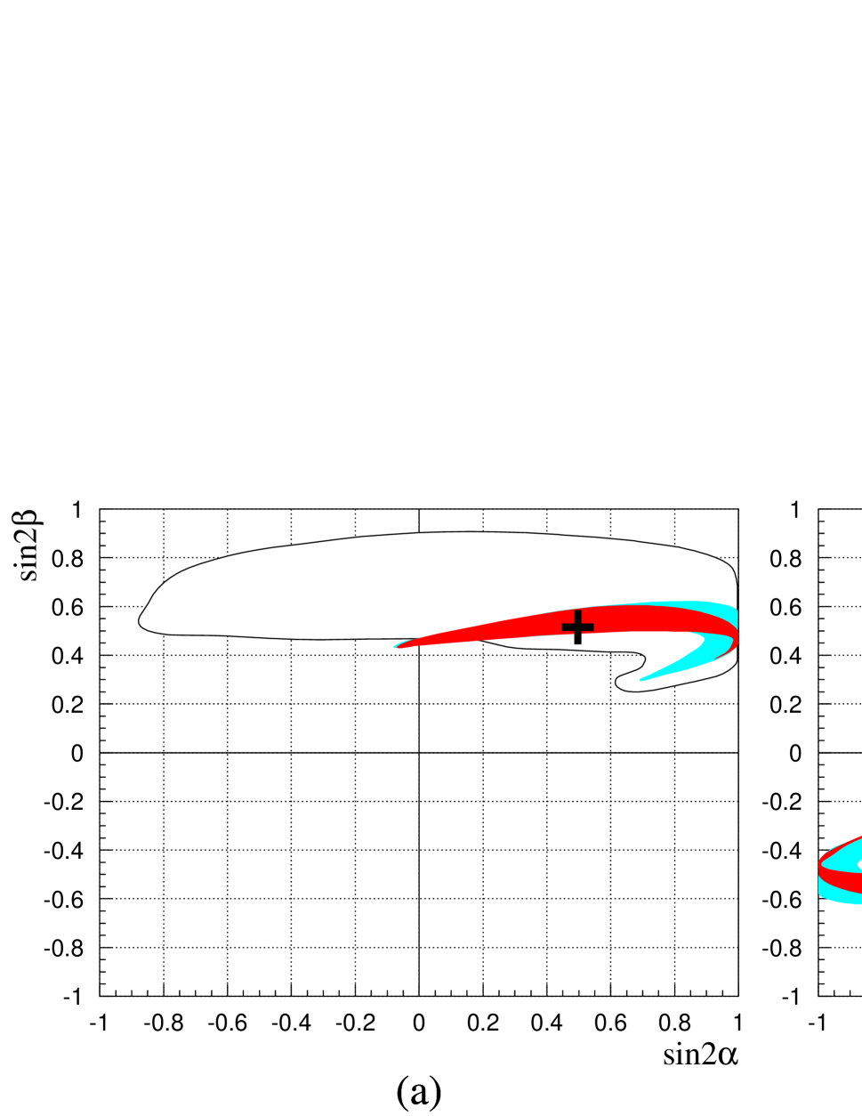
Figure 2: (a) 90% contour plots from the constrained fit ($\epsilon_{K}$ and $\Delta m_{B_{d}}$ included) for the SM (white area), the unified U(2) theories (light and dark shaded area), the model of sect. 6 with free phases (darker area) and with maximal phases (cross); (b) as in Fig. 2a from the unconstrained fit ($\epsilon_{K}$ and $\Delta m_{B_{d}}$ excluded)

At the same time, one obtains $m_{u}/m_{d}=0.76^{+0.10}_{-0.16}$ and $m_{u}/m_{d}=0.76^{+0.14}_{-0.22}$ in the constrained and unconstrained fits respectively. These values can be compared with $m_{u}/m_{d}=0.553\pm 0.043$, as obtained from chiral perturbation theory and some supplementary hypothesis [18].

6 An explicit SO(10)$\times$U(2) model

6.1 Definition and basic formulae

Within the stated assumptions, everything that has been said so far is general and is based on an operator analysis. In this section we describe an explicit SO(10)$\times$U(2) model. One purpose for this is to show that the $Q$ problem can be solved. This requires a model where all the corrections of relative order $\epsilon$ to Eqs. (8,9,10) are fully under control. In turn, this will allow us to detail the numerical fit of the known data and the predictions for several observables in flavor physics.

We seek a special realization of the superpotential in Eqs. (34,35,36,37) generated from a renormalizable theory, where the non-renormalizable operators arise from the exchange of heavy vector-like families (the so called “Froggatt-Nielsen” fields). A minimum choice involves one doublet under U(2), $\chi^{a}+\overline{\chi}_{a}$, transforming as $16+\overline{16}$ under SO(10). The most general, renormalizable, invariant superpotential involving these vector multiplets, the usual chiral multiplets, the Higgs ten-plet, the flavon fields $\phi^{a}({\bf 45})$, $S^{ab}({\bf 45})$, $A^{ab}({\bf 1})$ and the adjoint fields $\Sigma_{X}$ and $\Sigma_{Y}$, introduced in section 4, is

$$f=\psi_{3}H\psi_{3}+\chi^{a}H\psi_{a}+\overline{\chi}_{a}(M\chi^{a}+\Sigma_{X}\chi^{a}+\Sigma_{Y}\chi^{a}+\phi^{a}\psi_{3}+S^{ab}\psi_{b}+A^{ab}\psi_{b})$$ (53)

where, as usual, dimensionless couplings and SO(10) contractions are left understood.

On integrating out the heavy $\chi^{a}+\overline{\chi}_{a}$ states, one generates, from the diagrams shown in Fig. 3, a particular case of the superpotential (34,35,36,37). With respect to this general form, the term bilinear in the field $\phi^{a}$ is absent and only some contractions of the SO(10) indices occur. Also important is the fact that the superpotential (34,35,36,37) contains an infinite tower of $(\Sigma_{X}/M)^{n}$-operators, which are all under control in this case. This is welcome, in view of the fact, already mentioned, that $\left\langle\Sigma_{X}\right\rangle/M$ is not far from unity. In the following we treat $\left\langle\Sigma_{X}\right\rangle/M$ exactly and we give explicit formulae to first order in $\left\langle\Sigma_{Y}\right\rangle/M$, but we control the size of the higher order terms.

Figure 3: Diagrams generating the Yukawa coupling superpotential in the SO(10)$\times$U(2) model

To be able to write down explicit forms for the Yukawa matrices in this case, we only need to know the SO(10) properties of the U(2) doublet $\phi^{a}$. For the time being we take it to be an SO(10)-adjoint with its vev point in a generic SU(3)$\times$SU(2)$\times$U(1)-preserving direction $T$, so that $\left\langle\phi^{2}\right\rangle\equiv\left\langle\phi\right\rangle T$.

Following the line of the discussion in the previous section, it is straighforward to write down explicit expressions for the Yukawa matrices. After trivial rescalings, one gets

$$\halign to=0.0pt{\@eqnsel\hskip\@centering$\displaystyle{#}$&\global\@eqcnt\@ne\hskip 2\arraycolsep\hfil${#}$\hfil& \global\@eqcnt\tw@\hskip 2\arraycolsep$\displaystyle{#}$\hfil&\llap{#}\cr 0.0pt plus 1000.0pt$\displaystyle{\lambda^{U} &10.0pt\hfil${=&10.0pt$\displaystyle{\left(\begin{array}[]{ccc}0&\epsilon'\rho&0\\ -\epsilon'\rho&\epsilon\rho&r T_{u}\epsilon\\ 0&r T_{Q}\epsilon&1\end{array}\right)\lambda\\ \lambda^{D} &\hbox to0.0pt{\hss=&\left(\begin{array}[]{ccc}0&\epsilon^{\prime}&0\\ -\epsilon^{\prime}&\epsilon&rxT_{d}\epsilon\\ 0&rT_{Q}\epsilon&1\end{array}\right)\xi\\\lambda^{E}&=&\left(\begin{array}[]{ccc}0&\epsilon^{\prime}&0\\ -\epsilon^{\prime}&3\epsilon&rxT_{L}\epsilon\\ 0&rT_{e}\epsilon&1\end{array}\right)\xi&(54)\cr}}}}}$$

where

$$\halign to=0.0pt{\@eqnsel\hskip\@centering$\displaystyle{#}$&\global\@eqcnt\@ne\hskip 2\arraycolsep\hfil${#}$\hfil& \global\@eqcnt\tw@\hskip 2\arraycolsep$\displaystyle{#}$\hfil&\llap{#}\cr 0.0pt plus 1000.0pt$\displaystyle{&10.0pt\hfil${\displaystyle r=\frac{\left\langle\phi\right\rangle}{\left\langle S\right\rangle},\qquad x=\frac{1+\alpha}{1-3\alpha},\qquad\rho=-\frac{5}{16}\frac{\beta}{\alpha}\frac{1-3\alpha}{1+\alpha},&10.0pt$\displaystyle{\\ &\hbox to0.0pt{\hss\displaystyle\alpha\propto\frac{\left\langle\Sigma_{X}\right\rangle_{u}}{M},\qquad\beta\propto\frac{\left\langle\Sigma_{Y}\right\rangle_{u}}{M}&&(55)\cr}}}}}$$

and the normalization of $T$ is immaterial since it can be reabsorbed in $r$.

These Yukawa matrices have to be compared with the general form given in Eqs. (38,39). Notice that $\rho=\rho^{\prime}$ and that all the coefficients $x_{i}$, $y_{i}$ of order unity are now determined by the parameters $r$ and $x$. In particular, all combinations of dimensionless couplings occurring in the diagrams of Fig. 3 have been rescaled away. By redefining the phases of the matter superfields, it is possible to make the parameters $\lambda$, $\xi$, $\epsilon^{\prime}$ and $r$ real and positive. In general $\rho$, $x$ and $\epsilon$ are complex, so that, from now on

$$\rho\rightarrow\rho e^{i\hat{\alpha}},\quad x\rightarrow xe^{i\hat{\beta}},\quad\epsilon\rightarrow\epsilon e^{i\hat{\gamma}}$$ (56)

with $\rho$ real.

6.2 Solving the $Q$-problem

For any choice of $T$ it is now possible to use Eq. (3) to make a fit of the data. Before doing that, let us discuss again the problem of the corrections to the GJ relation (9). Notice that Eqs. (8) and (10), which we have used in sect. 5, remain unchanged.

As a consequence of the diagonalization of (3) in the 23 sector, Eq. (9) gets modified as

$$\frac{m_{\mu}}{m_{\tau}}=3\frac{m_{s}}{m_{b}}\left(1-{m_{d}\over m_{s}}\right)+\frac{m_{\mu}}{m_{\tau}}\Delta$$ (57)

where $(m_{\mu}/m_{\tau})\Delta$ is an additional contribution that depends, in particular, on the choice of $T$. From Eqs. (44,45), after specialization to (3), it follows that

$$|\frac{m_{\mu}}{m_{\tau}}\Delta|\leq x\epsilon^{2}r^{2}\left|T_{e}T_{L}-3T_{d}T_{Q}\right|=6x\epsilon^{2}r^{2}\left|T_{u}T_{Q}\right|,$$ (58)

where we have used $T_{L}=-3T_{Q}$ and $T_{d}+T_{e}=-2T_{u}$. From Eq (46), the parameter $x$ can be bound as

$$x\left|\frac{T_{d}}{T_{u}}\right|\leq\left(\frac{|V_{cb}|_{G}}{|T_{u}|\epsilon r}+1\right).$$ (59)

while the combination $\epsilon r$ can be obtained from $m_{c}/m_{t}|_{G}$ by means of Eq (43), where the term proportional to $\rho^{\prime}=\rho$ can be safely neglected for the purposes of this discussion. Therefore, from (58),

$$|\Delta|\leq\Delta_{\rm max}\equiv 6\left(\frac{m_{c}}{m_{t}}\right)_{G}^{1/2}\left(|V_{cb}|_{G}\left|\frac{T_{Q}}{T_{u}}\right|^{1/2}+\left(\frac{m_{c}}{m_{t}}\right)_{G}^{1/2}\right)\left|\frac{T_{u}}{T_{d}}\right|\left/\frac{m_{\mu}}{m_{\tau}}\right.$$ (60)

where the inequality is saturated for maximal phases.

Using (57) instead of (9) gives

$$\frac{m_{s}}{m_{d}}=25\cdot(1-2\Delta)$$ (61)

instead of (18), so that, from (17),

$$Q=25\cdot\frac{1-2\Delta}{\sqrt{1-\frac{m^{2}_{u}}{m^{2}_{d}}}}$$ (62)

To see the consistency of this expression with $Q=22.7\pm 0.08$, we plot in Fig. 4a the contours of $Q_{\rm min}\equiv Q(\Delta=\Delta_{\rm max})$ as function of $m_{u}/m_{d}$ and of a parameter $\theta$ which defines the general superposition of SO(10) generators: $T=X\cos\theta+Y\sin\theta$. This plot is only weakly sensitive to the values of $m_{c}$, $m_{t}$, $|V_{cb}|$, $\alpha_{s}(M_{Z})$, then fixed to their central values. As apparent from this figure, $Q$ as low as $22.7\pm 0.08$ can be obtained if $T=Y$ or $T=B-L$ for values of $m_{u}/m_{d}$ compatible with $|V_{ub}/V_{cb}|$, plotted in Fig. 4b. This is confirmed and made explicit by the overall fit discussed in the next subsection.

Figure 4: (a) contour plot of $Q_{\rm min}$ versus $m_{u}/m_{d}$ and $\theta$ in $T=X\cos\theta+Y\sin\theta$ for central values of $m_{c}$, $m_{t}$, $|V_{cb}|$, $\alpha_{s}(M_{Z})$; (b) $|V_{ub}/V_{cb}|$ versus $m_{u}/m_{d}$ for $\alpha_{s}(M_{Z})=0.117\pm 0.003$ and central values of $m_{b}$, $m_{c}$, $Q$

6.3 Parameter fit

A general fit of the data can be made based on Eqs. (40–47), specialized as in (3) with $T={Y}$ or $T={B-L}$. By a usual analysis, $\xi$ and $\lambda$ are determined by $m_{t}$ and $m_{\tau}$, allowing a prediction for $m_{b}$ in terms of $\alpha_{s}$ and $\tan\beta$.

For the renormalization rescalings [21], we use in particular

$$\frac{m_{b}}{m_{\tau}}=\frac{\eta_{b}}{\eta_{\tau}}\prod_{a}\frac{\zeta^{d}_{a}}{\zeta^{e}_{a}}\frac{1}{y_{t}}$$ (63)

where $\eta_{b}$, $\eta_{\tau}$ are the scaling factors from the weak scale to low energy, $\zeta^{d,e}_{a=1,2,3}$ are the gauge couplings renormalizations from the GUT scale to the weak scale and $y_{t}$ is the scaling factor, still from the GUT to the weak scale, due to the top Yukawa coupling. Eq. (63) is appropriate for the low $\tan\beta$ case, to which we stick in the following. One motivation for this is to be sure that the weak scale threshold corrections mentioned in section 3.3 do not invalidate the analysis.

The 16 observables in Table 3 depend on 14 parameters: the 10 free flavor parameters, the ratio of the two electroweak vevs $v_{2}/v_{1}$, $\alpha_{s}$, $\sqrt{B}f_{B}$ and $B_{K}$, so that the fit has 2 degrees of freedom. Having fixed the more precisely measured quantities to their central values, the other 6 observables are then fitted by varying the 4 remaining independent parameters (which we choose to be $\alpha_{s}$, $m_{u}/m_{d}$, $\cos(\hat{\alpha}-\hat{\gamma})$ and $\cos\hat{\beta}$). One should note that the errors in the input observables are mostly theoretical.

The results of the fit are shown in Tables 5 and 6 respectively for the parameters of the model, as defined in Eqs. (3,56) with $T={Y}$ and for the 6 input physical observables whose central values are allowed to vary. The fit does not determine the relative sign of $\sin(\hat{\alpha}-\hat{\gamma})$ and $\sin(\hat{\beta}+\hat{\gamma})$, but this ambiguity does not affect in a significant way any of the observables listed in Table 5 and 6.

$$\begin{array}[]{||c|c|c||}\hline\cr&\mbox{free phases}&\mbox{max phases}\\ \hline\cr\chi^{2}_{\rm min}/\mbox{d.o.f.}&0.67/2&2.1/5\\ \hline\cr\epsilon&0.0162^{+0.0013}_{-0.0008}&0.0174\pm 0.0002\\ \rho&0.0201\pm 0.006&0.0205\pm 0.001\\ \epsilon^{\prime}&0.00414&0.00414\\ r(T_{u}T_{Q})^{1/2}&1.95^{+0.31}_{-0.22}&2.10\pm 0.07\\ x&2.56^{+0.4}_{-1.1}&1.20\pm 0.035\\ \hline\cr\cos(\hat{\alpha}-\hat{\gamma})&0.22^{+0.19}_{-0.33}&0\\ \cos(\hat{\beta}+\hat{\gamma})&-0.95^{+0.55}_{-0}&-1\\ \cos\hat{\beta}&0.96^{+0.04}_{-0.06}&+1\\ \hline\cr\end{array}$$

Table 5: Parameters of the model, as determined from the fit, for $T={Y}$ with free phases or maximal phases

$$\begin{array}[]{||c|c|c|c||}\hline\cr&\mbox{inputs}&\mbox{free}&\mbox{max}\\ \hline\cr m_{s}/\rm\,MeV&175\pm 55&158\pm 28&155\pm 6\\ |V_{cb}|&0.038\pm 0.004&0.0391\pm 0.0025&0.0407\pm 0.002\\ |V_{ub}/V_{cb}|&0.08\pm 0.02&0.075^{+0.003}_{-0.012}&0.0611\pm 0.001\\ \sqrt{B}f_{B}/\rm\,MeV&200\pm 40&179^{+14}_{-10}&187\pm 8.5\\ B_{K}&0.8\pm 0.2&0.84^{+0.18}_{-0.14}&0.91\pm 0.15\\ \alpha_{s}&0.117\pm 0.006&0.119\pm 0.005&0.114\pm 0.001\\ \hline\cr\end{array}$$

Table 6: Results of the fit for $T={Y}$ with free phases or maximal phases

The fit with $T={B-L}$ gives results which are all within the uncertainties quoted in Table 5, 6.

As apparent from Table 5, all the values of the phases $\hat{\alpha}$, $\hat{\beta}$, $\hat{\gamma}$ are compatible with being maximal. At least for $\hat{\beta}$ and $\hat{\gamma}$ this is clearly indicated by the fit itself and it is suggestive of spontaneous CP violation. With this in mind, we have made a fit with all phases fixed at maximal values, $\hat{\alpha}=\pi/2$, $\hat{\beta}=0$, $\hat{\gamma}=\pi$ for $T=Y$. In this case, having still fixed all the inputs without an asterisk in Table 3 at their central values, only $\alpha_{s}$ remains as free parameter to fit the six observables in Table 6. Although this procedure may require improvements in the determination of the errors, which may be underestimated, the success of this fit is apparent from Tables 5, 6. In turn, this allows a determination of the CKM matrix with a small uncertainty in each of the parameters, even smaller than in the general case discussed in the previous section. This is also shown in Fig 2a, 2b, both for the case of free phases and for the case of maximal phases. As to the value of $m_{u}/m_{d}$, this is essentially unchanged from the general case when the phases are left free, whereas, for maximal phases, $m_{u}/m_{d}=0.606\pm 0.022$.

7 Conclusions

We have studied supersymmetric theories of flavor based on a flavor group U(2), with breaking pattern $\mbox{U(2)}\stackrel{{\scriptstyle\epsilon}}{{\rightarrow}}\mbox{U(1)}\stackrel{{\scriptstyle\epsilon^{\prime}}}{{\rightarrow}}0$, and symmetry breaking parameters $\epsilon\approx m_{s}/m_{b}$ and $\epsilon^{\prime}\approx\sqrt{m_{d}m_{s}/m_{b}^{2}}$. These parameters are sufficiently small that the quark and lepton mass matrices are dominated by terms up to linear order in $\epsilon$ and $\epsilon^{\prime}$, and must therefore arise from just 4 types of interactions: $\psi_{3}\psi_{3}H+(1/M)(\psi_{3}\phi^{a}\psi_{a}+\psi_{a}S^{ab}\psi_{b}+\psi_{a}A^{ab}\psi_{b})H$, with $S^{ba}=+S^{ab}$ and $A^{ba}=-A^{ab}$. Allowing the most general breaking of U(2) to U(1), by $\left\langle S^{22}\right\rangle,\left\langle\phi^{2}\right\rangle$ of order $\epsilon$, and assuming that the final U(1) is broken only by $\left\langle A^{12}\right\rangle$ of order $\epsilon^{\prime}$, a simple symmetry origin is found for a highly successful texture. This symmetry structure also solves the supersymmetric flavor-changing problem, while strongly suggesting that the exchange of superpartners at the weak scale will lead to observable rare flavor-changing and CP violating effects in future experiments. It is interesting that such a simple symmetry structure simultaneously provides a very constrained structure for the Yukawa matrices, and an acceptable form for the scalar mass matrices.

U(2) and its hierarchical breaking, $\mbox{U(2)}\stackrel{{\scriptstyle\epsilon}}{{\rightarrow}}\mbox{U(1)}\stackrel{{\scriptstyle\epsilon^{\prime}}}{{\rightarrow}}0$, are sufficient to qualitatively understand all the observed small fermion mass ratios and mixing angles, except the large $m_{t}/m_{b}$ ratio and the observation that the mass hierarchies in the up sector are larger than those in the down and charged lepton sectors. However, the combination of U(2) and grand unified symmetries allow a symmetry understanding for the large $m_{t}/m_{c}$ and $m_{c}/m_{u}$ hierarchies, which involve a small symmetry breaking parameter, $\rho$, the ratio of the SU(5) breaking scale to the UV cutoff of the theory. Furthermore, these symmetries enforce a correlation between these mass hierarchies and the mass relations $m_{\mu}=3m_{s}$ and $m_{e}m_{\mu}/m_{\tau}^{2}=m_{d}m_{s}/m_{b}^{2}$ at the unification scale – these mass relations are a necessary consequence of requiring large $m_{t}/m_{c}$ and $m_{c}/m_{u}$ ratios. In Tables 1 and 2 we give qualitative expressions for the 13 flavor observables of the standard model in terms of 4 small parameters $\epsilon,\epsilon^{\prime},\rho$ and $\xi$, a Higgs mixing parameter which allows large $m_{t}/m_{b}$. Hence unified U(2) theories give 9 approximate relations. Of these 9 relations, 5 are precise, receiving corrections which are higher order in the symmetry breaking parameters. These are the relations (15) and (16) for $|V_{ub}/V_{cb}|$ and $|V_{td}/V_{ts}|$, which follow purely from the texture dictated by the U(2) symmetry, and the three unified mass relations (8), (9) and (10) for $m_{b},m_{s},m_{d}$ in terms of $m_{\tau},m_{\mu},m_{e}$.

These results follow from a general operator analysis and apply in a wide class of unified U(2) theories. In section 3 we described a class of SU(5) theories, while in sections 4.2 and 4.3 we discussed two classes of SO(10) theories, distinguished by the SO(10) transformation properties of $\phi^{a},S^{ab}$ and $A^{ab}$. All these theories lead to the same constrained form for the Yukawa matrices, which successfully accounts for the known quark and lepton masses and mixings, provided the CKM unitarity triangle is constrained so that $\sin 2\alpha$ and $\sin 2\beta$ lie in the shaded (dark+light) region of Figure 2. This is a crucial prediction of the unified U(2) theories. The unified U(2) theories also predict $m_{u}/m_{d}=0.35$–$0.90$ at 90% confidence level.

The light quark and lepton masses, and the non-trivial structure for the CKM matrix, arise from non-renormalizable operators of the expansion in the effective theory. In section 6 we propose a specific SO(10) model in which these non-renormalizable operators are generated by the exchange of a U(2) doublet of heavy vector generations. This is the simplest unified U(2) theory that we know. The Yukawa matrices at the unification scale feel SU(5) breaking only via the mass of the heavy vector generations and the orientations of the $\phi$ and $S$ vevs, which transform as SO(10) adjoints. When fit to the data, this theory produces a somewhat tighter prediction for the CKM unitarity triangle compared to the general unified theories, as seen from the dark shaded region of Figure 2.

An interesting feature of this model is that the fit to the data shows that the three independent physical phases which enter the Yukawa matrices are constrained to be close to multiples of $\pi/2$, suggesting a spontaneous origin for CP violation via the vevs which break the flavor and grand unified symmetries. In this case, the Yukawa matrices depend on just 7 parameters, and a fit to data produces precise predictions for $\sin 2\alpha$, $\sin 2\beta$ and $|V_{ub}/V_{cb}|$. The scalar mass matrices of this model are more restricted than in the general unified U(2) theories, allowing a calculation of the mixing matrices at gaugino vertices. The resulting predictions for the supersymmetric contributions to flavor and CP violating observables will be reported elsewhere.

Acknowledgments

This work was supported in part by the Director, Office of Energy Research, Office of High Energy and Nuclear Physics, Division of High Energy Physics of the U.S. Department of Energy under Contract DE-AC03-76SF00098, in part by the National Science Foundation under grant PHY-95-14797 and in part by the U.S. Department of energy under contract DOE/ER/01545–700.

References

• [1] H. Georgi, H. R. Quinn, and S. Weinberg, Phys. Rev. Lett. 33, 451 (1974);\\ S. Dimopoulos, S. Raby, and F. Wilczek, Phys. Rev. D24, 1681 (1981);\\ S. Dimopoulos and H. Georgi, Nucl. Phys. B193, 150 (1981);\\ L. E. Ibanez and G. G. Ross, Phys. Lett. 105B, 439 (1981).
• [2] M. S. Chanowitz, J. Ellis, and M. K. Gaillard, Nucl. Phys. B128, 506 (1977).
• [3] L. E. Ibanez and C. Lopez, Phys. Lett. 126B, 54 (1983);\\ H. Arason et al., Phys. Rev. Lett. 67, 2933 (1991);\\ A. Giveon, L. J. Hall, and U. Sarid, Phys. Lett. 271B, 138 (1991).
• [4] R. Gatto, G. Sartori, and M. Tonin, Phys. Lett. 28B, 128 (1968);\\ N. Cabibbo and L. Maiani, Phys. Lett. 28B, 131 (1968);\\ S. Weinberg, in A Festschrift for I.I. Rabi, edited by L. Motz, New York Academy of Sciences, 1977.
• [5] H. Georgi and C. Jarlskog, Phys. Lett. 86B, 297 (1979).
• [6] J. Harvey, P. Ramond, and D. Reiss, Phys. Lett. 92B, 309 (1980).
• [7] G. W. Anderson, S. Raby, S. Dimopoulos, L. J. Hall, and G. D. Starkman, Phys. Rev. D49, 3660 (1994).
• [8] L.J. Hall and L. Randall, Phys. Rev. Lett. 65 2939 (1990);\\ M. Dine, R. Leigh and A. Kagan, Phys. Rev. D48 4269 (1993);\\ Y. Nir and N. Seiberg, Phys. Lett. B309 337 (1993);\\ P. Pouliot and N. Seiberg, Phys. Lett. B318 169 (1993);\\ M. Leurer, Y. Nir and N. Seiberg, Nucl. Phys. B398 319 (1993);\\ M. Leurer, Y. Nir and N. Seiberg, Nucl. Phys. B420 319468 (1994);\\ D. Kaplan and Schmaltz, Phys. Rev. D49 3741 (1994);\\ A. Pomarol and D. Tommasini, CERN-TH/95-207;\\ L.J. Hall and H. Murayama, Phys. Rev. Lett. 75 3985 (1995);\\ P. Frampton and O. Kong, IFP-725-UNC (1996);\\ E. Dudas, S. Pokorski and C.A. Savoy, Saclay T95/094, hep-ph/9509410;\\ C. Carone, L.J. Hall and H. Murayama, LBL-38047 (1995);\\ R. Barbieri, G. Dvali, and L. J. Hall, Phys. Lett. B377, 76 (1996);\\ Y. Kawamura, H. Murayama and M. Yamaguchi, Phys. Rev. D51 1337 (1995);\\ N. Arkani-Hamed, H.-C. Cheng and L. J. Hall, LBL 37893 (1995); LBL 37894 (1996);\\ R. Barbieri and L. J. Hall, LBL–38381, hep-ph 9605224;\\ Z. Berezhiani, INFN FE 06–96, hep-ph/9609342.
• [9] M. Dine, W. Fischler, and M. Srednicki, Nucl. Phys. B189 575 (1981);\\ S. Dimopoulos and S. Raby, Nucl. Phys. B192 353 (1981);\\ M. Dine and W. Fischler, Phys. Lett. B110 227 (1982);\\ M. Dine and M. Srednicki, Nucl. Phys. B202 238 (1982);\\ M. Dine and W. Fischler, Nucl. Phys. B204 346 (1982);\\ L. Alvarez-Gaumé, M. Claudson, and M. Wise, Nucl. Phys. B207 96 (1982);\\ C.R. Nappi and B.A. Ovrut, Phys. Lett. B113 175 (1982);\\ S. Dimopoulos and S. Raby, Nucl. Phys. B219 479 (1983).
• [10] R. Barbieri and L. J. Hall, Phys. Lett. B338, 212 (1994).
• [11] R. Barbieri, L. J. Hall, and A. Strumia, Nucl. Phys. B445, 219 (1995); ibid. B449, 437 (1995); S. Dimopoulos and L. J. Hall, Phys. Lett. B344, 185 (1995).
• [12] R. Barbieri, Proceedings of the Erice Summer School 1995.
• [13] For a most recent analysis, see F. Gabbiani, E. Gabrielli, A. Masiero and L. Silvestrini, ROM2F/96/21 and references therein.
• [14] A. Pomarol and D. Tommasini, [8].
• [15] R. Barbieri, G. Dvali and L. J. Hall, [8]; R. Barbieri and L. J. Hall, [8].
• [16] L. J. Hall and A. Rasin, Phys. Lett. B315, 164 (1993).
• [17] T. Blazek, S. Raby, and S. Pokorski, Phys. Rev. D52, 4151 (1995).
• [18] H. Leutwyler, CERN–TH/96–25, hep-ph/9602255
• [19] V. Lucas and S. Raby, Phys. Rev. D54, 2261 (1996).
• [20] R. N. Cahn, I. Hinchliffe, and L. J. Hall, Phys. Lett. 109B, 426 (1982).
• [21] For a recent analysis, see, e.g., V. Barger, M. Berger, and P. Ohmann, Phys. Rev. D47, 1093 (1993).
• [22] C. Froggatt and H. B. Nielsen, Nucl. Phys. B147, 277 (1979);\\ Z. G. Berezhiani, Phys. Lett. 129B, 99 (1983); ibid. 150B, 177 (1985);\\ S. Dimopoulos, Phys. Lett. 129B, 417 (1983).
• [23] Particle Data Group, Phys. Rev. D54, 1 (1996).