$\epsilon$ expansion analysis of very weak first-order transitions
in the cubic anisotropy model: Part I

Abstract

The cubic anisotropy model provides a simple example of a system with an arbitrarily weak first-order phase transition. We present an analysis of this model using $\epsilon$-expansion techniques with results up to next-to-next-to-leading order in $\epsilon$. Specifically, we compute the relative discontinuity of various physical quantities across the transition in the limit that the transition becomes arbitrarily weakly first-order. This provides a useful test-bed for the application of the $\epsilon$ expansion in weakly first-order transitions.

I Introduction

The cubic anisotropy model is a simple two-scalar model that, for a certain range of parameters, has a phase transition with similarities to the finite-temperature phase transition of electroweak theory in the early universe. More generally, it provides a simple prototype for systems that have weak, fluctuation-induced, first-order phase transitions [1, 2]. In ref. [3], we and our collaborators discuss in detail the similarities and dissimilarities with the electroweak transition (noted earlier by Alford and March-Russel [4]) and described how the cubic anisotropy model is a good testing ground for analytic techniques that claim to distinguish between second-order and weakly first-order phase transitions. In particular, the model can be used to study $\epsilon$ expansion methods, which we have previously applied to the electroweak case [5]. This paper presents the details of calculating $\epsilon$ expansions for weakly first-order phase transitions in the cubic anisotropy model. A better overview of the motivation, a summary of our $\epsilon$ expansion results, and a comparison against numerical Monte Carlo simulations [6] may be found in ref. [3].

Our goal will be to compute the relative discontinuity of various quantities (the specific heat, susceptibility, and correlation length) across the phase transition when one has an extremely weak first-order transition. Specifically, we will compute ratios such as $\chi_{+}/\chi_{-}$ where $\chi_{\pm}$ are the susceptibilities on either side of the transition. This was originally done at leading order in $\epsilon$ by Rudnick some twenty years ago [1]. We have extended the calculation to next-to-leading order (NLO) for the correlation length and next-to-next-to-leading order (NNLO) for the susceptibility ratio. A next-to-leading order calculation for the specific heat ratio is performed in a companion paper [7].

A Three-dimensional reduction and the cubic anisotropy model

Before introducing the cubic anisotropy model, we shall very briefly review the connection between phase transitions in thermal quantum field theory and those in classical statistical mechanics. For definiteness, consider the topical example of electroweak theory. In studying the electroweak transition, one starts with a 3+1 dimensional SU(2) gauge-Higgs theory at finite temperature. Schematically, the Euclidean action is of the form

$$S=\int_{0}^{\beta}d\tau\int d^{d}x\>\left\{{\displaystyle{1\over 2}}\,|D\phi|^{2}+{\displaystyle{1\over 4}}\,F^{2}-{\displaystyle{\mu^{2}\over 2}}\,|\phi|^{2}+{\displaystyle{\lambda\over 4!}}\,|\phi|^{4}+\cdots\right\}\,,$$ (1)

(with gauge-fixing terms omitted). $\beta$ is the inverse temperature, and $d=3$ is the number of spatial dimensions. If the correlation length at the transition is large compared to the inverse temperature (which is generally the case), one may simplify the study of equilibrium properties of the transition by integrating out the dynamics of the Euclidean time direction. This yields an effective three-dimensional theory that describes the long distance physics of the transition and which may be precisely matched, order by order in coupling constants, to the original theory:

$$S_{\rm eff}=\beta\int d^{d}x\>\left\{{1\over 2}\,|D\phi|^{2}+{1\over 4}\,F^{2}+{t\over 2}\,|\phi|^{2}+{\lambda_{\rm eff}\over 4!}\,|\phi|^{4}+\cdots\right\}\,.$$ (2)

For a review, see refs. [5, 8]. There is no need to go into detail here, except to note that the mass-squared $t$ of the Higgs in the effective theory has the form

$$t=-\mu^{2}+c\,g^{2}T^{2}+\cdots\,,$$ (3)

for some constant $c$. The fact that $t$ becomes positive as the temperature $T$ increases drives the restoration of manifest SU(2) symmetry at high temperature. The action (2) describes a classical statistical mechanics problem in three spatial dimensions, where $S_{\rm eff}$ is to be interpreted as $\beta H$.

In this work, we will not study the three-dimensional theory (2), but will instead examine a simpler three-dimensional theory consisting of two scalar fields known as the cubic anisotropy model. In a more general form, the cubic anisotropy model is an O($n$) symmetric scalar model of $n$ real scalar fields, to which is added an interaction that breaks O($n$) symmetry down to hyper-cubic symmetry [1, 2]. The action is

$$S=\int d^{d}x\>\left\{{1\over 2}\left|\partial\vec{\phi}\right|^{2}+{t\over 2}\left|\vec{\phi}\right|^{2}+\kappa u\left|\vec{\phi}\right|^{4}+\kappa v\sum_{i}\phi_{i}^{4}\right\}\,.$$ (4)

(Note that the overall $\beta$ in (2) can be absorbed by a rescaling of $\phi$.) We will ultimately be interested in the simplest case, $n=2$. The parameters $u$ and $v$ are dimensionless coupling constants, and $\kappa$ is a dimensionful normalization which we will fix later. The phase transition of interest occurs as the parameter $t$ is varied. At tree level, the transition appears to be second-order, with hyper-cubic symmetry spontaneously broken for $t<0$ and restored for $t>0$. As we shall review, however, the effect of higher-order corrections on the nature of the transition cannot be ignored.

B The $\epsilon$ expansion

In second-order phase transitions, the correlation length diverges at the transition and physics near the transition is dominated by large infrared fluctuations which cannot be treated perturbatively. One way of summarizing this for a theory like the cubic anisotropy model is to note that, since the couplings $\kappa u$ and $\kappa v$ of the theory have non-trivial mass dimension $4{-}d=1$, the dimensionless loop expansion parameter $R$ must, by dimensional analysis, be of the form

$$R~{}~{}\sim~{}~{}\hbox{($\kappa u$ or $\kappa v$)}~{}~{}\times~{}~{}\hbox{(some correlation length)}^{4-d}\,,$$ (5)

which diverges with the correlation length. In first-order phase transitions, the correlation length is finite, but perturbation theory can still fail if the correlation length is large enough that $R\gtrsim 1$. We shall refer to such a situation as a weakly first-order transition. In this paper, our goal will be to study the arbitrarily weak limit $R\to\infty$.

The $\epsilon$ expansion is based on generalizing $d{=}3$ spatial dimensions to $d{=}4{-}\epsilon$ dimensions. When $\epsilon$ is small, one can systematically remedy the problems of perturbation theory by using suitable renormalization-group (RG) improved perturbation theory. Computing to some order in RG-improved perturbation theory corresponds to computing to some order in $\epsilon$. At the end of the day, one sets $\epsilon{\to}1$ in the resulting truncated series. In some cases this is known to give quite good results.

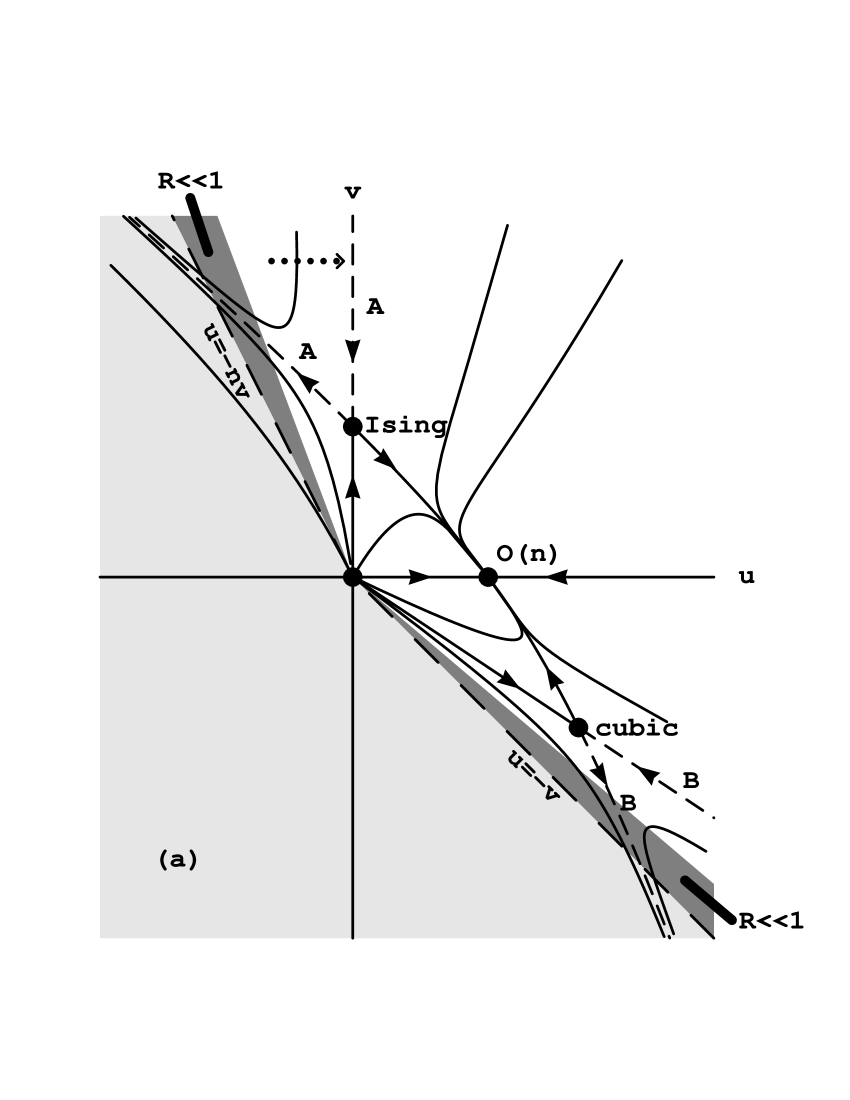
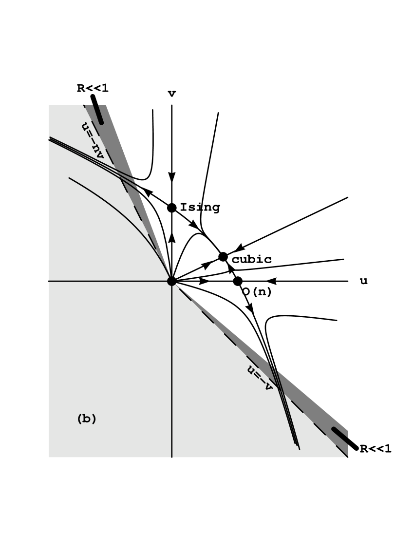
FIG. 1.: Renormalization group flow into the infrared of $(u,v)$ for small $\epsilon$ and (a) $n<n_{\rm c}=4+O(\epsilon)$, or (b) $n>n_{\rm c}$. The lightly shaded region is the domain in which the tree-level potential (4) is unbounded below. The more heavily shaded “wedges” show the regions in which perturbation theory is reliable. In the left-hand figure (a), the special trajectories labeled A and B will be a focus of attention. These are the limiting trajectories for theories which approach the Ising or cubic fixed points arbitrarily closely before flowing off toward the classical instability line. Such theories have arbitrarily weak first order phase transitions.

Fig. 1 shows the renormalization group flow, for small $\epsilon$, of the dimensionless couplings $u$ and $v$ of the cubic anisotropy model as one moves to longer distance scales. The lightly shaded region, delimited by the lines $u=-nv$ and $u=-v$, designates the range of couplings where the tree-level potential of (4) is unbounded below. For $v=0$, the cubic anisotropy model reduces to an O($n$) model, which has a second-order phase transition associated with the infrared fixed point marked “O($n$)”. For $u=0$, the model (4) reduces to $n$ uncoupled copies of a basic quartic scalar field theory, which is in the same universality class as the Ising model. The associated fixed point is marked “Ising” in fig. 1. Besides the Gaussian fixed point at $u{=}v{=}0$, there is another fixed point known as the cubic fixed point. All of these fixed points occur at couplings of $O(\epsilon)$, and so the couplings may be treated as small and perturbative when $\epsilon\ll 1$.

The stability or instability of these fixed points depends on the number $n$ of scalar fields. For $n<n_{\rm c}=4+O(\epsilon)$ (which encompasses our main case of interest, $n{=}2$), the O($n$) fixed point is infrared stable, as shown in fig. 1(a), while the Ising and cubic fixed points have an unstable direction and correspond to tricritical points. A theory whose couplings lie between the lines running from the origin to the Ising and cubic fixed points, respectively, will flow at large distances to the O($n$) fixed point and so will have a second-order transition with O($n$) symmetric critical behavior. A theory with couplings outside of this region (and not on the critical lines bounding this region) does not flow to any weakly coupled infrared-stable fixed point, and so might be expected to have a first-order phase transition. This is indeed the case. As discussed by Rudnick [1], and as we shall review below, the criteria $R\ll 1$ for the success of perturbation theory (known as the Ginsburg criteria) is satisfied for couplings very close to the region of tree-level instability, designated by the heavy shaded regions in Fig. 1. In these $R\ll 1$ regions, one indeed finds that perturbation theory reliably predicts a first-order transition. The renormalization group flow then shows that any theory whose couplings are outside the boundary of the basin of attraction of the O($n$) fixed point is equivalent to a theory with couplings having $R\ll 1$, and so will have a first-order transition. The lines from the origin through the Ising and cubic tricritical points are therefore boundaries separating theories with first- and second-order transitions.

The case of $n>n_{\rm c}$ is shown in fig. 1(b). The O($n$) and cubic fixed points exchange roles relative to the $n<n_{\rm c}$ case.

Now consider a sequence of theories with first-order transitions, such as those indicated by the dotted line near the top of fig. 1a, which approach the Ising line $u{=}0$. The correlation length at the transition can then be made arbitrarily large, since for $u{=}0$ it is infinite. The renormalization group trajectory approaches the dashed line in fig. 1a labeled trajectory A. This limiting trajectory first flows into the Ising fixed point along the line $u{=}0$, and then flows away from the Ising fixed point in the unstable direction toward the region of classical instability. A similar limit for the tricritical behavior of the cubic fixed point gives trajectory B. This is the limit we will take to obtain arbitrarily weak first-order transitions in the cubic anisotropy model. For $n=2$, trajectories A and B are equivalent because a redefinition of $\vec{\phi}$ by a $45^{\circ}$ internal rotation,

$$(\phi_{1},\phi_{2})\to{1\over\sqrt{2}}(\phi_{1}+\phi_{2},\phi_{1}-\phi_{2})\,,$$ (6)

leaves the Lagrangian (4) in the same form but with

$$(u,v)\to(u+{\textstyle{3\over 2}}v,-v)\,.$$ (7)

This means that theories below the $u$ axis in fig. 1(a) are, for $n{=}2$, related by the mapping (7) to theories above the axis.

We will therefore compute properties of the transition, for small $\epsilon$, on trajectory B. This is easiest to do by following the trajectory into the perturbative region $R\ll 1$. Throughout this paper, we focus on the flow away from the cubic fixed point. For $n{=}2$, the final results for physical quantities must be the same as for flow from the Ising fixed point. For other $n$, the flow from the Ising fixed point could be analyzed similarly, but we have not bothered to do so.

In the next section, we fix notations and renormalization scheme conventions. In section III, we review the leading-order analysis of the susceptibility ratio $\chi_{+}/\chi_{-}$, which was originally carried out by Rudnick [1]. The most straightforward derivation uses a calculation of the one-loop effective potential and the explicit one-loop RG equations. After reviewing this calculation, we show that explicit knowledge of the one-loop potential and RG equations was not actually necessary. In section IV we extend the calculation to next-to-leading order. This calculation does require the explicit one-loop potential and RG equations, but we show that explicit knowledge of the two-loop corrections (which would be used in the most straightforward derivation) is not required. Section V computes the next-to-leading order result for the correlation length ratio $\xi_{+}^{2}/\xi_{-}^{2}$. Then, in section VI, we finally extend our calculation of $\chi_{+}/\chi_{-}$ to next-to-next-to-leading order, which requires a non-trivial ring-diagram resummation of perturbation theory, the explicit two-loop potential, and the explicit two-loop RG equations. Finally, section VII summarizes our results. A review of the leading-order result for the flow of the couplings $(u,v)$, originally derived by Rudnick [1], as well as details of the two-loop potential, are left to appendices.

II Notation and Conventions

We will use dimensional regularization for loop calculations in $d=4{-}\epsilon$ dimensions and a renormalization scheme closely related to modified minimal subtraction ($\overline{\rm MS}$). Specifically, the bare Lagrangian is

$${\cal L}_{\rm bare} = {\textstyle{1\over 2}}Z_{\phi}^{2}\,|\partial\vec{\phi}|^{2}+V_{\rm bare}(\vec{\phi})$$ (8)

with

$$V_{\rm bare}(\vec{\phi}) = \bigl{(}{\cal N}\!\mu^{\epsilon}\bigr{)}^{-1}\Lambda+{\textstyle{1\over 2}}Z_{m^{2}}Z_{\phi}^{2}m^{2}|\vec{\phi}|^{2}+{\textstyle{1\over 4!}}{\cal N}\!\mu^{\epsilon}Z_{\phi}^{4}\left[Z_{u}u|\vec{\phi}|^{4}+Z_{v}v\sum_{i}\phi_{i}^{4}\right]\,,$$ (9)

and

$${\cal N} = (4\pi)^{d/2}\,\Gamma\!\left(\textstyle{d\over 2}{-}1\right),$$ (10)

and where all renormalization constants have the form

$$Z_{i} = 1+{z_{i1}(u,v)\over\epsilon}+{z_{i2}(u,v)\over\epsilon^{2}}+\cdots\,.$$ (11)

Note that we have rescaled our couplings and $\Lambda$ by an additional factor of $(4\pi)^{2}$ compared to the typical convention in particle theory. The additive constant $\Lambda$ is irrelevant to the calculation of the susceptibility or correlation length ratios and may be ignored, but it will be important for the specific heat ratio computed in ref. [7]. Note that we have relabeled the parameter $t$ as $m^{2}$, which is the typical notation used in particle theory. But it should be kept in mind that variation of $m^{2}$ really represents variation of temperature in the underlying physical problems of interest.

The susceptibility $\chi$ is defined by adding a linear term $h\phi$ to the Lagrangian and defining

$$\chi\equiv\lim_{h\to 0}{d\langle\phi\rangle\over dh}\,.$$ (12)

The normalization and regularization of the $h\phi$ term is not important because we will ultimately only be interested in the ratio $\chi_{+}/\chi_{-}$, where it cancels out.

III Review of leading-order analysis

Two things are needed to analyze the transition: (a) the location of some point $(u,v)$ along the portion of the trajectory within the perturbative regime, and (b) a perturbative analysis at that point. Technically, it is easiest to choose the point where the trajectory intersects the line $u=-nv$ or $u=-v$, where the tree-level potential first becomes unstable. (The full, effective potential remains stable, as it must, since it is invariant under changes of renormalization scale.) We shall call this point $(u_{*},v_{*})$.

The value of $(u_{*},v_{*})$ turns out not to affect the leading-order calculation of $\chi_{+}/\chi_{-}$; so we shall proceed for the moment without it. (The value of the couplings does affect the leading-order results of other ratios, such as the specific heat ratio $C_{+}/C_{-}$ [1, 7].)

At tree level the transition appears second-order. For $m^{2}>0$, the minimum of the tree-level potential is at $\vec{\phi}{=}0$. For $m^{2}<0$, it is along an “edge”, $\vec{\phi}\propto(1,0,0,\cdots)$, if $v<0$, and along a “diagonal”, $\vec{\phi}\propto(1,1,1,\cdots)$, if $v>0$. Rather than discussing the entire structure of the effective potential $V(\vec{\phi})$, it will generally be sufficient simply to consider its behavior in the relevant direction. For flow from the cubic fixed point ($v<0$), attention can be restricted to an edge. The tree-level potential $V_{0}$ then becomes

$$V_{0}(\vec{\phi})\to V_{0}(\phi) = {1\over 2}m^{2}\phi^{2}+{1\over 4!}{\cal N}\!\mu^{\epsilon}(u+v)\phi^{4}\,,$$ (13)

where

$$\vec{\phi} = (\phi,0,0,\cdots)\,.$$ (14)

At the instability line, $u{=}{-}v$ and hence the quartic interaction term disappears along the edge.

To see the first-order nature of the transition, one must consider the effect of the first loop correction. This is just the Coleman-Weinberg effect [10]. For the sake of definiteness, and because we need the results later on, we shall go through the explicit calculation of the one-loop corrections to the effective potential. However, after the fact, we shall show that an explicit calculation was actually unnecessary for computing $\chi_{+}/\chi_{-}$ at leading order.

A The one-loop potential

The one-loop contribution to the effective potential is

$$V_{1}(\vec{\phi})={\cal I}(m_{\rm a}^{2})+(n{-}1)\,{\cal I}(m_{\rm b}^{2})~{}~{}+~{}~{}(\hbox{counter-terms})\,,$$ (15)

where $m_{\rm a}^{2}$ and $m_{\rm b}^{2}$ are the eigenvalues of the curvature of the tree-level potential $V_{0}(\vec{\phi})$ evaluated at $\vec{\phi}$, and the one-loop integral ${\cal I}(z)$ is

$${\cal I}(z)={\textstyle{1\over 2}}\,{\rm tr}\ln(-\partial^{2}+z)=-{\textstyle{1\over 2}}\,(4\pi)^{-d/2}\,\Gamma\left(-\textstyle{d\over 2}\right)z^{d/2}\,.$$ (16)

Along an edge, we have

$$m_{\rm a}^{2} = m^{2}+{\textstyle{1\over 2}}{\cal N}\!\mu^{\epsilon}(u+v)\,\phi^{2}\,,$$ (18)

$$m_{\rm b}^{2} = m^{2}+{\textstyle{1\over 6}}{\cal N}\!\mu^{\epsilon}u\,\phi^{2}\,,$$ (19)

which are the curvatures parallel and orthogonal to the edge, respectively.

Now take $u=-v$ to fix ourselves on the tree-level instability line. It is notationally convenient to express the potential in terms of

$$M^{2}\equiv{\textstyle{1\over 6}}\mu^{\epsilon}{\cal N}u\,\phi^{2},$$ (20)

and one finds

$${\cal N}\!\mu^{\epsilon}V_{0}(\phi) = \Lambda+3u^{-1}m^{2}M^{2}\,,$$ (21)

$${\cal N}\!\mu^{\epsilon}V_{1}(\phi) = \left[{m^{4}\over 2\epsilon}-{2\pi\mu^{\epsilon}\,m^{d}\over d(d{-}2)\sin(\pi\epsilon/2)}\right]+(n{-}1)\left[{(m^{2}{+}M^{2})^{2}\over 2\epsilon}-{2\pi\mu^{\epsilon}\,(m^{2}+M^{2})^{d/2}\over d(d{-}2)\sin(\pi\epsilon/2)}\right].$$ (22)

For the moment, we’re only working to leading-order in $\epsilon$, so we can take the limit $\epsilon{\to}0$ to find:

$${\cal N}\!\mu^{\epsilon}(V_{0}+V_{1})=\Lambda + 3u^{-1}m^{2}M^{2}+{1\over 4}\,m^{4}\left[\,\ln\!\left(m^{2}\over\mu^{2}\right)-{3\over 2}\right]$$ (23)

$$+ {(n{-}1)\over 4}\,(m^{2}+M^{2})^{2}\left[\,\ln\!\left(m^{2}{+}M^{2}\over\mu^{2}\right)-{3\over 2}\right]+O(\epsilon)\,.$$ (24)

As one varies $m^{2}$, this potential describes a first-order transition which occurs at an $m^{2}{\not=}0$. If it weren’t for the one-loop corrections, the transition would be second-order and occur at $m^{2}{=}0$. Since couplings are $O(\epsilon)$, one then expects that $m^{2}$ at the transition is small if $\epsilon$ is small. We shall indeed see a posteriori that

$${m^{2}\over M^{2}}\sim O(\epsilon)$$ (25)

when the order parameter $\phi$ is the same order of magnitude as its value in the asymmetric phase. So in this range of $\phi$ we can drop $m$ compared to $M$ and find

$${\cal N}\!\mu^{\epsilon}(V_{0}+V_{1})=\Lambda+3u^{-1}m^{2}M^{2}+M^{4}\left[C_{11}\ln\!\left(M^{2}\over\mu^{2}\right)+C_{10}\right]+O(\epsilon M^{4},m^{2}M^{2},m^{4})\,,$$ (26)

where

$$C_{11}={n{-}1\over 4}\,,\qquad C_{10}=-{3\over 2}\,C_{11}\,.$$ (27)

The above approximation to the potential has two degenerate minima when

$$m^{2}=m_{1}^{2}\equiv{C_{11}\,u\,\mu^{2}\over 3}\exp\left(-1-{C_{10}\over C_{11}}\right)={n{-}1\over 12}\,u\,\mu^{2}e^{1/2}\,,$$ (28)

and the value of $M$ at the asymmetric minima is

$$M^{2}=M_{1}^{2}\equiv\mu^{2}\exp\left(-1-{C_{10}\over C_{11}}\right)=\mu^{2}e^{1/2}\,.$$ (29)

As promised, $m_{1}^{2}/M_{1}^{2}\sim O(u)\sim O(\epsilon)$. The curvatures at the origin and at the asymmetric minima are

$$1/\chi_{+} \propto \left.{\partial^{2}V(\phi)\over\partial\phi^{2}}\right|_{\phi=0}={\textstyle{1\over 6}}{\cal N}\!\mu^{\epsilon}uV^{\prime\prime}(0)~{}~{}~{}\>=m^{2}\,[1+O(\epsilon)]\,,$$ (30)

$$1/\chi_{-} \propto \left.{\partial^{2}V(\phi)\over\partial\phi^{2}}\right|_{\phi=\phi_{1}}={\textstyle{1\over 6}}{\cal N}\!\mu^{\epsilon}uV^{\prime\prime}(M_{1})=2m^{2}\,[1+O(\epsilon)]$$ (31)

(where $V^{\prime}(M)\equiv\partial V(M)/\partial M$, etc.). Thus,

$${\chi_{+}\over\chi_{-}}=2+O(\epsilon)\,.$$ (32)

B Avoiding one-loop details

In the preceding derivation, the final result for $\chi_{+}/\chi_{-}$ did not, in fact, depend on the values (27) of the constants $C_{11}$ and $C_{10}$. So we could have arrived at the same result simply knowing the form (26) of the one-loop potential in the limits $\epsilon{\to}0$, $u{=}{-}v$, and $m^{2}/M^{2}\sim O(\epsilon)$. But this form just follows from (a) the existence of the renormalization group, which produces a single power of $\ln\mu$ at one-loop order, and (b) the fact that $M$ is the only relevant dimensionful parameter if $m$ is negligible. The logarithm must therefore be $\ln(M/\mu)$ in our approximation. If we had understood a priori the independence of the result on $C_{11}$ and $C_{10}$, we could have avoided doing the explicit one-loop calculation. Generalizations of the following arguments will later save us from the need for two-loop calculations at next-to-leading order, and three-loop calculations at next-to-next-to-leading order.

The independence from $C_{10}$ may be understood as follows. The only parameters that final results can depend on are the dimensionless couplings $(u_{*},v_{*})$ and the corresponding renormalization scale $\mu$. Other parameters, such as $m^{2}$ and the scalar expectation $M$ have been solved for and eliminated by requiring that we be at the transition and in one or the other phase. If our final result is a dimensionless ratio, such as $\chi_{+}/\chi_{-}$ or $C_{+}/C_{-}$, it must then be independent of $\mu$ and can depend only on $(u_{*},v_{*})$. So the answer can’t change even if we arbitrarily change $\mu$ in (26) while holding $(u_{*},v_{*})$ fixed. (This is different from a simple statement of RG invariance, which would involve changing $(u,v)$ in a compensating manner when changing $\mu$.) Such a change in $\mu$ (at lowest order) is equivalent to varying $C_{10}$, and so dimensionless ratios do not depend on $C_{10}$.

The coefficient $C_{11}$ of the logarithm is determined by the one-loop renormalization group. However, as noted above, it is not needed for $\chi_{+}/\chi_{-}$. The reason is that, at leading order, the result (32) is independent of the couplings $(u_{*},v_{*})$. So the result would be the same if we redefined $(u,v)$ by $(u,v)\to(xu,xv)$ for some constant $x$. This redefinition does not take us off the line $u{=}{-}v$, but it does change the coefficients of the one-loop $\beta$-functions and therefore changes $C_{11}$. The leading-order result for $\chi_{+}/\chi_{-}$ must therefore be independent of $C_{11}$. This simplification doesn’t occur for $C_{+}/C_{-}$, which turns out to be proportional to $u_{*}$ at leading order [1, 7].

As a prelude to our later higher-order analysis, it will be useful to sketch the renormalization group determination of $C_{11}$. The one-loop RG equation for the effective potential in the cubic anisotropy model is

$$\left(\mu{\partial\over\partial\mu}+\beta_{u}{\partial\over\partial u}+\beta_{v}{\partial\over\partial v}+\beta_{m^{2}}\,m^{2}{\partial\over\partial{m^{2}}}+\gamma_{\phi}\,\phi{\partial\over\partial\phi}+\beta_{\Lambda}{\partial\over\partial\Lambda}\right)V=0\,,$$ (33)

where

$$\beta_{u}(u,v,\epsilon) = -\epsilon u+\bar{\beta}_{u}(u,v)\,,$$ (35)

$$\beta_{v}(u,v,\epsilon) = -\epsilon v+\bar{\beta}_{v}(u,v)\,,$$ (36)

with

$$\bar{\beta}_{u}(u,v) = \beta^{(1)}_{u}+O(u^{3},v^{3})\,,\qquad\beta^{(1)}_{u}=u\left({\textstyle{1\over 3}}(n{+}8)\,u+2v\right)\,,$$ (38)

$$\bar{\beta}_{u}(u,v) = \beta^{(1)}_{v}+O(u^{3},v^{3})\,,\qquad\beta^{(1)}_{v}=v\left(4u+3v\right)\,,$$ (39)

$$\beta_{m^{2}}(u,v) = \beta^{(1)}_{m^{2}}+O(u^{2},v^{2})\,,\qquad\beta^{(1)}_{m^{2}}={\textstyle{1\over 3}}(n{+}2)\,u+v\,,$$ (40)

$$\gamma_{\phi}(u,v) = O(u^{2},v^{2})\,.$$ (41)

For the susceptibility, we are only interested in the $\phi$ dependence of the potential, and the running of $\Lambda$ will be irrelevant. As it turns out, we will also not need $\beta_{m^{2}}$ or $\gamma_{\phi}$ below.

The renormalization group flow does not map the line $u{+}v=0$ onto inself. Consequently, to apply the RG equation, one must retain the $v$ dependence of the tree-level potential (13) rather than specializing from the outset to $u{=}{-}v$. Working at $\epsilon{=}0$, one easily finds that the RG equation is satisfied by

$$V_{0}+V_{1} = V_{0}-\left\{{\textstyle{1\over 2}}\,\beta^{(1)}_{m^{2}}\,m^{2}\phi^{2}+{\textstyle{1\over 4!}}\,{\cal N}[\beta^{(1)}_{u}+\beta^{(1)}_{v}]\,\phi^{4}\right\}\ln\mu$$ (43)

$$\qquad\qquad{}+(\hbox{$\mu$-independent})+O(\epsilon^{2}V)\,.$$

Taking $u{=}{-}v$ (and neglecting $m^{2}$ relative to $M^{2}$) then gives

$$C_{11}={3\over 4u^{2}}\left(\beta^{(1)}_{u}+\beta^{(1)}_{v}\right)\biggl{|}_{u{=}{-}v}\,,$$ (44)

which agrees with (27). In later sections, this same RG method will be used to determine $\mu$-dependent terms in the two- and three-loop contributions to the effective potential.

C Scale hierarchies and subtleties at higher orders

As we shall see, the preceding tricks for simplifying calculations will generalize to higher orders in $\epsilon$ as well. Leading-order results for generic ratios require only explicit knowledge of the tree-level potential and the one-loop renormalization group, and $\chi_{+}/\chi_{-}$ doesn’t even need the latter. Next-to-leading order calculations generically require the explicit one-loop potential and the two-loop renormalization group, although $\chi_{+}/\chi_{-}$ needs only the one-loop renormalization group. Next-to-next-to-leading order generically requires the two-loop potential and the three-loop renormalization group, and so forth.

FIG. 2.: A sequence of diagrams of the same order in $\epsilon$ in the asymmetric phase. Solid lines represent heavy ($m_{\rm b}$) degrees of freedom; light lines represent the light ($m_{\rm a}$) degrees of freedom.

There is a subtlety, however, in the simplistic assumption that each successive order in $\epsilon$ requires exactly one more order in the loop expansion of the effective potential. The source of this subtlety is the ratio of scales $m^{2}/M^{2}\sim O(\epsilon)$ in the asymmetric phase. Fig. 2 shows a sequence of diagrams, with arbitrarily many loops (starting at 3 loops), which are all the same order in $\epsilon$ in the asymmetric phase. These diagrams consist of multiple “ring” corrections to the light (mass $m^{2}$) mode due to interactions with the heavy (mass $M^{2}$) modes. The outer loop is dominated by momenta of order $m$, and the cost of adding an additional ring is

$$O(u^{2}\phi^{2}/m^{2})=O(uM^{2}/m^{2})=O(1)\,.$$ (45)

This particular problem could be handled diagrammatically by resumming the light propagator to incorporate all one-loop heavy rings. A more elegant way to think about it is in the language of the renormalization group. At distances large compared to $1/M$ in the asymmetric phase, our scalar theory should be replaced by an effective theory consisting of only the light degree of freedom. The mass of the light scalar in the effective theory will be its original mass $m$ plus corrections from integrating out the heavy modes.

The free energy in this light effective theory will be of order $m^{4}$. Comparison to (26) then reveals that it will only be important at next-to-next-to-leading order. If only working to NLO, one can ignore the need for this resummation in the asymmetric phase.

IV NLO analysis of $\chi_{+}/\chi_{-}$

A The effective potential: asymmetric phase

Going one order beyond the previous analysis requires consideration of (a) two-loop contributions to the effective potential, and (b) corrections to the $\epsilon\to 0$ and $m^{2}/M^{2}\to 0$ limits we took of the one-loop potential. For the latter, we can simply expand the general one-loop potential (22) to the desired order:

$${\cal N}\!\mu^{\epsilon}(V_{0}+V_{1}) = \Lambda+3u^{-1}m^{2}M^{2}+M^{4}\left[C_{11}\ln\!\left(M^{2}\over\mu^{2}\right)+C_{10}\right]+{\cal N}\!\mu^{\epsilon}\delta V_{1}+O(\epsilon^{2}V)_{\rm asym}\,,$$ (46)

with

$${\cal N}\!\mu^{\epsilon}\,\delta V_{1} = \epsilon\,M^{4}\left[-{\textstyle{1\over 4}}C_{11}\ln^{2}\!\left(M^{2}\over\mu^{2}\right)-{\textstyle{1\over 2}}C_{10}\ln\!\left(M^{2}\over\mu^{2}\right)+C_{\epsilon 10}\right]$$ (47)

$$+ m^{2}M^{2}\left[\,2C_{11}\ln\!\left(M^{2}\over\mu^{2}\right)-2C_{11}\right],$$ (48)

and

$$C_{\epsilon 10} = -\left({7\over 8}+{\pi^{2}\over 12}\right)C_{11}\,.$$ (49)

The subscript “${\rm asym}$” is a reminder of the assumption $m^{2}/M^{2}\sim O(\epsilon)$ in the error estimate, which is valid only in the asymmetric phase.

For the two-loop contribution, we may take $\epsilon{=}0$ and ignore $m^{2}$ altogether. The renormalization group requires the contribution to have the form

$${\cal N}\!\mu^{\epsilon}V_{2}=uM^{4}\left[\,C_{22}\ln^{2}\!\left(M^{2}\over\mu^{2}\right)+C_{21}\ln\!\left(M^{2}\over\mu^{2}\right)+C_{20}\right]+O(\epsilon^{2}V)_{\rm asym}\,.$$ (50)

As in the leading-order calculation, we will not actually need to compute all three parameters.

The first simplification is to note that rescaling $\mu$ by

$$\mu\to\mu\,(1+xu)$$ (51)

in $V_{0}+V_{1}+V_{2}$, while holding all couplings fixed, changes $C_{20}$ at this order but nothing else. Therefore dimensionless ratios cannot depend on $C_{20}$ at NLO. Similarly, a change such as

$$\mu\to\mu\,(1+x\epsilon)$$ (52)

would change $C_{\epsilon 10}$ and nothing else, so we never actually needed its value (49) for a NLO calculation.

We could determine all the other constants in (50) by requiring the potential to satisfy the RG equation at two loops. However, analogous to what happened at leading order, we will not need all of these coefficients for $\chi_{+}/\chi_{-}$. It is sufficient to apply the RG equation at one loop order, as given by (33–III B). However, we do need the one-loop potential for general $(u,v)$ without the restriction $u{=}{-}v$. Returning to (15) and (16), one easily finds

$${\cal N}\mu^{\epsilon}\,(V_{0}+V_{1}) = \Lambda+{3\over 2}\,{u{+}v\over u^{2}}\,M^{4}+{9\over 4}\,{(u{+}v)^{2}\over u^{2}}\,M^{4}\left[\ln\!\left(3\,(u{+}v)\,M^{2}\over u\,\mu^{2}\right)-{3\over 2}\right]$$ (54)

$$\qquad\qquad\qquad\qquad{}+{(n{-}1)\over 4}\,M^{4}\left[\ln\!\left(M^{2}\over\mu^{2}\right)-{3\over 2}\right]+O(\epsilon^{2}V)_{\rm asym}\,.$$

Applying the one-loop RG equation, and then setting $u{=}{-}v$, determines

$$C_{22}={n{+}2\over 6}C_{11}\,.$$ (55)

It is also worth noting that it was unnecessary to compute explicitly the $O(\epsilon)$ correction to $V_{1}$ given by the first term of (48), because the coefficients of the logs in that correction are determined by the RG equation as well, arising from the explicit $\epsilon$ in (*‡ ‣ III B). This observation will substantially simplify the analogous calculation when we later proceed to NNL order.

To find the asymmetric phase susceptibility $\chi_{-}$, we now need at next-to-leading order both the value of $m^{2}$ at the transition and of $M^{2}$ in the asymmetric phase. Perturb around the one-loop solutions (28) and (29) by writing

$$V=V_{(1)}+\delta V\,,\qquad m^{2}=m_{1}^{2}+\delta m^{2}\,,\qquad M=M_{1}+\delta M\,,$$ (56)

where $V_{(1)}$ is the one-loop $\epsilon{=}0$ approximation (26) to the effective potential and

$$\delta V=\delta V_{1}+V_{2}$$ (57)

as parameterized in (48) and (50). By linearizing the equations $V(M){=}V(0)$ and $V^{\prime}(M){=}0$ that determine the asymmetric phase expectation $M$ at the transition point, one finds

$$\delta m^{2} = -{\cal N}\mu^{\epsilon}\,{u\over 3}\left.\left(\delta V(M)-\delta V(0)\over M^{2}\right)\right|_{M_{1},m_{1}}+O(\epsilon^{2}m^{2})\,,$$ (58)

and

$$\delta M = -{M^{2}\over V_{(1)}^{\prime\prime}}\,{\partial\over\partial M}\!\left.\left(\delta V\over M^{2}\right)\right|_{M_{1},m_{1}}+O(\epsilon^{2}M)\,.$$ (59)

The fractional shift in $1/\chi_{-}$ is

$$\left({d^{2}V_{(1)}\over dM^{2}}\right)^{-1}\delta{d^{2}V\over dM^{2}}=\left.\left({\partial^{2}\,\delta V\over\partial M^{2}}+{6\,\delta m^{2}\over{\cal N}\mu^{\epsilon}u}+\delta M\,{\partial^{3}V_{(1)}\over\partial M^{3}}\right)\right|_{M_{1},m_{1}}.$$ (60)

Putting in the explicit form for $\delta V$, we obtain

$$m^{2} = m_{1}^{2}\left[1+\left(-{5\over 16}-{C_{\epsilon 10}\over C_{11}}\right)\epsilon+\left({(n{-}4)\over 24}-{1\over 2}{C_{21}\over C_{11}}-{C_{20}\over C_{11}}\right)u+O(\epsilon^{2})\right]\,,$$ (61)

$$M^{2} = M_{1}^{2}\left[1+\left(-{13\over 16}-{C_{\epsilon 10}\over C_{11}}\right)\epsilon+\left(-{(3n{+}2)\over 8}-{3\over 2}{C_{21}\over C_{11}}-{C_{20}\over C_{11}}\right)u+O(\epsilon^{2})\right]\,,$$ (62)

$$1/\chi_{-} \propto \partial_{\phi}^{2}V(\phi)=2m^{2}\left[1-{1\over 2}\,\epsilon-{(n{-}13)\over 12}\,u+O(\epsilon^{2})\right]\,.$$ (63)

Note how all the dependence of $\partial_{\phi}^{2}V$ on $C_{\epsilon 10}$, $C_{21}$, and $C_{20}$ in the result (63) is hidden in the overall factor of $m^{2}$.

B The effective potential: symmetric phase

When examining the asymmetric phase, we made an expansion in $m^{2}/M^{2}=O(\epsilon)$. For the symmetric phase, where $M{=}0$, this is not a good approximation. The symmetric phase is easier, however, because one needs only one-loop contributions at $\epsilon{=}0$ for next-to-leading order results. Consider the one-loop potential (24). It gives

$$1/\chi_{+}\propto\partial_{\phi}^{2}V(0) = m^{2}\left\{1+{(n{-}1)\over 6}\,u\left[\ln\!\left(m^{2}\over\mu^{2}\right)-1\right]+O(\epsilon^{2})\right\}$$ (64)

$$= m^{2}\left\{1+{(n{-}1)\over 6}\,u\left[\ln\!\left({(n{-}1)\over 12}u\right)-{1\over 2}\right]+O(\epsilon^{2})\right\}\,.$$ (65)

Putting this together with the asymmetric phase result gives our NLO ratio

$${\chi_{+}\over\chi_{-}}=2\left[1-{1\over 2}\,\epsilon-{(n{-}1)\over 6}\,u_{*}\ln\!\left({(n{-}1)\over 12}u_{*}\right)+u_{*}\right]+O(\epsilon^{2})\,,$$ (66)

where we now explicitly remind ourselves that $u$ is to be evaluated at the point $(u_{*},v_{*})$. At leading order, we didn’t need to know $u_{*}$ at all for $\chi_{+}/\chi_{-}$. For next-to-leading order, we need to find the leading order value of $u_{*}$.

C $(u_{*},v_{*})$ at leading order

The one-loop RG equations for the couplings are

$$\mu{\partial u\over\partial\mu} = -\epsilon u+\beta^{(1)}_{u}(u,v)\,,$$ (68)

$$\mu{\partial v\over\partial\mu} = -\epsilon v+\beta^{(1)}_{v}(u,v)\,,$$ (69)

where $\beta^{(1)}_{u}$ and $\beta^{(1)}_{v}$ are given in (III B). The explicit solution was found when $n{=}2$ by Rudnick [1] and generalized to other $n$ by Domany, et al. [11]. We review the derivation in Appendix A. The resulting trajectories are given by

$$v = \epsilon\,R(u/v,c)\,,$$ (70)

where

$$R(f,c) \equiv {\lambda^{2}\,f^{-3}\over(n\lambda+1)(n\lambda+2)}\left[{(n\lambda+1)\over\lambda}f^{2}-2f+{2\over n}-{2c\over n}\left(1+{f\over\lambda}\right)^{-n\lambda}\right]\,,$$ (71)

$$\lambda \equiv {3\over 4-n}\,,$$ (72)

and each choice of the constant $c$ picks out a different trajectory. The trajectory that flows away from the cubic fixed point is $c=0$; the one flowing away from the Ising fixed point is $c=1$. The values of $(u,v)$ on the tree-level instability line are then

$$(u_{*},v_{*})=(u_{*},-u_{*})\,,\quad u_{*}=-\epsilon R(-1,0)={3(n^{2}+5n+3)\over n(n{+}2)(n{+}8)}\,\epsilon\,,$$ (73)

for flow from the cubic fixed point and

$$(u_{*},v_{*})=(-{\textstyle{1\over n}}v_{*},v_{*}),\;\;v_{*}=\epsilon R(-{\textstyle{1\over n}},1)={3n\over(n{+}2)(n{+}8)}\left[\textstyle 3n\left({4\over 3}(1{-}{1\over n})\right)^{-n\lambda}-(7n{+}2)\right]\epsilon,$$ (74)

for flow from the Ising fixed point. For $n{=}2$, these are

$$\left(\textstyle{51\over 80}\epsilon,-\textstyle{51\over 80}\epsilon\right)\quad\hbox{and}\quad\left(-\textstyle{51\over 160}\epsilon,\textstyle{51\over 80}\epsilon\right),$$ (75)

respectively, and are related by the mapping (7).

Our final, next-to-leading order result for $\chi_{+}/\chi_{-}$ is given by (66) and (73). For $n{=}2$ this yields

$${\chi_{+}\over\chi_{-}}=2\left[1-{17\over 160}\,\epsilon\ln\!\left(17\epsilon\over 320\right)+{11\over 80}\,\epsilon+O(\epsilon^{2})\right]\,.$$ (76)

The presence of an $\epsilon\ln\epsilon$ term is a feature that one does not encounter in $\epsilon$ expansions for critical exponents of second-order transitions. It arises here from the hierarchy of scales $m^{2}/M^{2}\sim\epsilon$ characterizing the physics of the asymmetric phase at the transition.

V NLO analysis of $\xi_{+}^{2}/\xi_{-}^{2}$

The correlation length $\xi$ is determined by the location of the pole of the two-point correlation. This is the solution $p^{2}=-\xi^{-2}$ to

$$p^{2}+m^{2}+\Pi(p^{2})=0\,,$$ (77)

where $\Pi(p^{2})$ is the (one-particle irreducible) self-energy. Since $m^{2}{+}\Pi(0)$ is another name for the susceptibility $1/\chi$, we can write

$$\xi^{-2}=\chi^{-1}+\left[\Pi(-\xi^{-2})-\Pi(0)\right]\,.$$ (78)

As we shall see, this equation can be solved by iteration, treating the second term, call it $\Delta\Pi$, as small. Hence, at leading order $\xi^{-2}$ is the same as $\chi^{-1}$ and is $O(m^{2})$. Fig. 3 shows the only one-loop graph that contributes to the momentum dependence of $\Pi(p^{2})$.

FIG. 3.: One loop diagram contributing to momentum-dependence of $\Pi$ in asymmetric phase.

In the symmetric phase, the expectation $\langle\phi\rangle$ is zero and so fig. 3 vanishes. The only mass scale is $m$ and so two-loop contributions to $\Delta\Pi$ would be order $O(u^{2}m^{2})=O(\epsilon^{2}\xi^{-2})$, which can be ignored at next-to-leading order.

In the asymmetric phase, the largest correlation length will be that associated with the degree of freedom $\phi_{1}$ along the edge, corresponding to $m_{a}^{2}=O(m^{2})$ in (16). For $u=-v$, this degree of freedom does not couple to itself, and the degrees of freedom running around the loop in fig. 3 are the heavier ones $\phi_{i}$ ($i\not=1$) associated with the mass scale $m_{\rm b}^{2}=O(M^{2})$. The momentum dependence $\Delta\Pi$ of fig. 3 is therefore $O(u\,p^{2})=O(u\,m^{2})=O(\epsilon\,\xi^{-2})$. As advertised, it can be treated as a perturbation. Explicit calculation in the $p^{2}\ll M^{2}$ limit gives

$$\Pi(p^{2})-\Pi(0)={(n{-}1)\over 18}\,u\,p\,^{2}+O(\epsilon^{2}m^{2})_{{\rm asym}}\,,$$ (79)

and so

$$\xi_{-}^{2} = \chi_{-}\left[\,1+{(n{-}1)\over 18}\,u+O(\epsilon^{2})\right]\,,$$ (80)

$$\xi_{+}^{2} = \chi_{+}\left[\,1+O(\epsilon^{2})\right]\,.$$ (81)

Combining with the result (66) for the susceptibility ratio gives

$${\xi_{+}^{2}\over\xi_{-}^{2}}=2\left[1-{1\over 2}\epsilon-{(n{-}1)\over 6}u_{*}\ln\!\left({(n{-}1)\over 12}u_{*}\right)-{(n{-}19)\over 18}u_{*}\right]+O(\epsilon^{2})\,.$$ (82)

Finally, inserting the $n{=}2$ value (75) of $u_{*}$ yields

$${\xi_{+}^{2}\over\xi_{-}^{2}}=2\left[\,1-{17\over 160}\,\epsilon\ln\!\left(17\epsilon\over 320\right)+{49\over 480}\,\epsilon+O(\epsilon^{2})\right]\,.$$ (83)

VI NNLO analysis of $\chi_{+}/\chi_{-}$

A The 2-loop renormalization group

Two-loop RG $\beta$-functions for the cubic anisotropy model may be easily extracted by following standard derivations in one-scalar models and replacing the overall couplings of each diagram by those appropriate for our two-scalar model. One finds

$$\bar{\beta}(u,v) = \beta^{(1)}+\beta^{(2)}+O(u^{4},v^{4})\,,$$ (84)

$$\gamma(u,v) = \gamma^{(2)}+O(u^{4},v^{4})\,,$$ (85)

with

$$\beta^{(2)}_{u} = -{(3n+14)\over 3}u^{3}-{22\over 3}u^{2}v-{5\over 3}uv^{2}\,,$$ (86)

$$\beta^{(2)}_{v} = -{(5n+82)\over 9}u^{2}v-{46\over 3}uv^{2}-{17\over 3}v^{3}\,,$$ (87)

$$\beta^{(2)}_{m^{2}} = -{5\over 6}\left[{(n{+}2)\over 3}u^{2}+2uv+v^{2}\right],$$ (88)

$$\gamma^{(2)}_{\phi} = -{(n{+}2)\over 36}u^{2}-{1\over 6}uv-{1\over 12}v^{2}\,.$$ (89)

B The effective potential: asymmetric phase

FIG. 4.: One-loop diagram contributing to effective light mass.

As discussed in section III C, the NNLO analysis of the effective potential in the asymmetric phase requires separating the light and heavy modes and doing a resummation of the heavy modes’ effect on the light ones. The effective mass $m_{\rm eff}$ of the light mode at distances large compared to $1/M$ can be found by explicitly computing the diagrams of fig. 4. More simply, it can be taken from the curvature of the one-loop potential (26) near the asymmetric minima (29):

$$m_{\rm eff}^{2}(M)=m^{2}+3{(u{+}v)\over u}M^{2}+(n{-}1)\,uM^{2}\left[{1\over 2}\ln\!\left(M^{2}\over\mu^{2}\right)-{1\over 6}\right]+O(\epsilon m^{2})\,.$$ (90)

The sub-leading $O(\epsilon m^{2})$ corrections to the above relationship are convention dependent: they depend on exactly how we want to define $m_{\rm eff}$. However, such sub-leading corrections to $m_{\rm eff}^{2}$ are not relevant at the order of interest.

The effective potential in the asymmetric phase is

$$V=V_{0}~{} + ~{}(V_{1}^{\rm heavy}+V_{1}^{\rm light}+\delta V_{1}^{\rm heavy}+\delta^{2}V_{1}^{\rm heavy})$$ (91)

$$+ ~{}(V_{2}^{\rm heavy}+\delta V_{2}^{\rm heavy})~{}+~{}V_{3}^{\rm heavy}~{}+~{}O(\epsilon^{3}V)_{\rm asym}\,,$$ (92)

where $V_{0}+V_{1}^{\rm heavy}$ and $\delta V_{1}^{\rm heavy}$ are given by (46) and (48). We have added the superscript “${\rm heavy}$” to indicate that these contributions come from the heavy modes. The next correction $\delta^{2}V_{1}^{\rm heavy}$ from the expansion of the second term in the one-loop potential (22) is

$${\cal N}\!\mu^{\epsilon}\,\delta^{2}V_{1}^{\rm heavy} = C_{11}\,m^{4}\ln\!\left(M^{2}\over\mu^{2}\right)+\epsilon\,m^{2}M^{2}\left[-{\textstyle{1\over 2}}\,C_{11}\ln^{2}\!\left(M^{2}\over\mu^{2}\right)+C_{11}\ln\!\left(M^{2}\over\mu^{2}\right)+C_{\epsilon m10}\right]$$ (93)

$$+ \epsilon^{2}M^{4}\left[{\textstyle{1\over 24}}\,C_{11}\ln^{3}\!\left(M^{2}\over\mu^{2}\right)+{\textstyle{1\over 8}}\,C_{10}\ln^{2}\!\left(M^{2}\over\mu^{2}\right)-{\textstyle{1\over 2}}\,C_{\epsilon 10}\ln\!\left(M^{2}\over\mu^{2}\right)+C_{\epsilon\epsilon 10}\right].$$ (94)

This can be justified either by explicit expansion or by application of the renormalization group. The new constant $C_{\epsilon\epsilon 10}$ will be irrelevant because it can be absorbed into a redefinition of $\mu$. The new constant $C_{\epsilon m10}$ may be extracted from explicit expansion of (24):

$$C_{\epsilon m10}=-\left(1+{\pi^{2}\over 6}\right)C_{11}\,.$$ (95)

The last piece of the one-loop potential we need is the contribution from the light modes, corresponding to the third term of (24). However, this contribution must be computed with the correct effective mass (90) so that

$${\cal N}\!\mu^{\epsilon}V_{1}^{\rm light}={1\over 4}\,m_{\rm eff}^{4}\left[\ln\!\left(m_{\rm eff}^{2}\over\mu^{2}\right)-{3\over 2}\right]\,.$$ (96)

As usual, this mass resummation is most easily accomplished by rewriting the light mass term of the Lagrangian as

$${\textstyle{1\over 2}}\,m^{2}\,\phi^{2}={\textstyle{1\over 2}}\,m_{\rm eff}^{2}\,\phi^{2}+{\textstyle{1\over 2}}\,(m^{2}{-}m_{\rm eff}^{2})\,\phi^{2}\,,$$ (97)

treating the first term on the right-hand side as part of the unperturbed Lagrangian and the second term as a perturbation. This perturbation will generate a new graph at NLO, shown in fig. 5.

FIG. 5.: Next-to-leading order contribution involving the effective mass counterterm $(m^{2}{-}m_{\rm eff}^{2})$.

For the two-loop potential, first consider the $\epsilon\to 0$ and $m\to 0$ limit of (50), which we now refer to as $V_{2}^{\rm heavy}$. For the current calculation, we will need to know all of the coefficients $\{\,C_{2i}\,\}$. $C_{21}$ may be determined by either explicit calculation or by applying the two-loop RG to the one-loop potential (54). The constant $C_{20}$, however, requires explicit calculation. The two-loop contributions are given the diagrams of fig. 6 combined with fig. 5.

FIG. 6.: Two-loop diagrams contributing to $V_{2}^{\rm heavy}$.

The details of the calculation are given in Appendix B, and one finds

$$C_{21}=-{(n{+}6)\over 3}\,C_{11}\,,\qquad C_{20}={(n{+}18)\over 6}\,C_{11}\,,$$ (98)

in addition to the previous result (55) for $C_{22}$.

The sub-leading corrections to $V_{2}^{\rm heavy}$ come from relaxing the $\epsilon{\to}0$ limit and remembering that the heavy mass (19) is $M^{2}+m^{2}$ instead of simply $M^{2}$. Expanding in $\epsilon$ and $m^{2}/M^{2}$ gives

$${\cal N}\mu^{\epsilon}\,\delta V_{2}^{\rm heavy} = u\,m^{2}M^{2}\left[{(n{-}1)\over 3}\,C_{11}\ln^{2}\!\left(M^{2}\over\mu^{2}\right)-{(n{+}4)\over 3}\,C_{11}\ln\!\left(M^{2}\over\mu^{2}\right)+C_{m20}\right]$$ (101)

$${}+\epsilon\,uM^{4}\Biggl{[}-{(n{+}2)\over 12}\,C_{11}\ln^{3}\!\left(M^{2}\over\mu^{2}\right)+{(3n{+}14)\over 12}\,C_{11}\ln^{2}\!\left(M^{2}\over\mu^{2}\right)$$

$$\qquad\qquad\qquad\qquad\quad-\left({n{+}10\over 3}+{(n{+}2)\over 36}\pi^{2}\right)C_{11}\ln\!\left(M^{2}\over\mu^{2}\right)+C_{\epsilon 20}\Biggr{]}\,,$$

where the coefficients of all the logs can be determined by requiring the full potential to be invariant under the two-loop RG. The constant $C_{\epsilon 20}$ will be irrelevant as it can be absorbed into a redefinition of $\mu$. The remaining constant, $C_{m20}$, is found by expansion of the explicit ($\epsilon{=}0$) two-loop potential, as described in Appendix B. One finds

$$C_{m20}=-{1\over 3}\,C_{11}\,.$$ (102)

Finally, the contribution of heavy modes to the three-loop potential has the form

$${\cal N}\!\mu^{\epsilon}V_{3}=u^{2}M^{4}\left[C_{33}\ln^{3}\!\left(M^{2}\over\mu^{2}\right)+C_{32}\ln^{2}\!\left(M^{2}\over\mu^{2}\right)+C_{31}\ln\!\left(M^{2}\over\mu^{2}\right)+C_{30}\right]+O(\epsilon^{3}V)_{\rm asym}\,.$$ (103)

We will only need $C_{33}$ and $C_{32}$ for $\chi_{+}/\chi_{-}$. ($C_{31}$ can be changed by a suitable redefinition of the couplings, and so cannot affect the physical ratio $\chi_{+}/\chi_{-}$.) The coefficients $C_{33}$ and $C_{32}$ can be determined by applying the two-loop RG to the full potential. To do so, we first need to relax the restriction $u{=}{-}v$ in our calculation of the two-loop potential. The analysis can be simplified a bit, however, in that we can treat $u{+}v$ as small and only keep terms linear in $u{+}v$. (That is because the RG derivative $\beta_{u}\partial_{u}+\beta_{v}\partial_{v}$ acting on $u{+}v$ does not give zero when $u=-v$, although the same operation on $(u{+}v)^{2}$ does yield zero.) Keeping only such terms in the $m{=}0$, $\epsilon{\to}0$ approximation to the potential gives the following analog to (54):

$${\cal N}\mu^{\epsilon}(V_{0}{+}V_{1}{+}V_{2}) = \Lambda+M^{4}\Biggl{\{}\left[C_{11}\ln\!\left(M^{2}\over\mu^{2}\right)\!+C_{10}\right]\!+u\left[C_{22}\ln^{2}\!\left(M^{2}\over\mu^{2}\right)\!+C_{21}\ln\!\left(M^{2}\over\mu^{2}\right)\!+C_{20}\right]$$ (106)

$$\qquad\qquad{}+{3\over 2}{(u{+}v)\over u^{2}}\!+(u{+}v)\!\left[-{C_{11}\over 2}\ln^{2}\!\left(M^{2}\over\mu^{2}\right)\!-3\,C_{11}\ln\!\left(M^{2}\over\mu^{2}\right)\!-{5\,C_{11}\over 2}\right]$$

$$\qquad\qquad{}+O\bigl{(}(u{+}v)^{2}\bigr{)}+O(\epsilon)\Biggr{\}}.$$

Combining with $V_{3}$, applying the RG, and then taking $u{=}{-}v$ yields

$$C_{33}={\textstyle{1\over 36}}\,(n^{2}+8)\,C_{11}\,,\qquad C_{32}=-{\textstyle{1\over 36}}\,(2n^{2}+45n+7)\,C_{11}\,.$$ (107)

C The effective potential: symmetric phase

In order to find the critical value of $m^{2}$, we must equate the free energy of the two phases. The asymmetric phase approximation (92) is not good in the $M{=}0$ symmetric phase because it relies on the approximation $m^{2}/M^{2}\sim O(\epsilon)$. We must compute the symmetric-phase free energy independently. At the order of interest, it is just the one-loop contribution (24):

$${\cal N}\!\mu^{\epsilon}V(0)=\Lambda+{n\over 4}\,m^{4}\left[\ln\!\left(m^{2}\over\mu^{2}\right)-{3\over 2}\right]+O\bigl{(}\epsilon^{3}M_{1}^{4}\bigr{)}\,.$$ (108)

For the NNLO susceptibility in the symmetric phase, we need the curvature of the two-loop potential at $M{=}0$. This is obtained by differentiating the general result (7) of Appendix B, and yields (130).

D $(u_{*},v_{*})$ at NLO

The NNLO result for $\chi_{+}/\chi_{-}$ will require a NLO value for $(u_{*},v_{*})$. Consider the one-loop result for the RG trajectories, (70) with $c=0$ or $1$, flowing from the tricritical points. Consider the solution for $u$ as a function of $f\equiv u/v$, and call it $u^{[1]}(f)$. Now look at the perturbation as we include higher loops. Start by making the rescaling

$$(u,v)=(\epsilon\,\bar{u},\epsilon\,\bar{v})\,,\qquad\mu=\bar{\mu}^{-1/\epsilon}\,,$$ (109)

which makes the $\epsilon$ expansion explicit in the RG equations:

$$\bar{\mu}{\partial\bar{u}\over\partial{\bar{\mu}}} = -\bar{u}+\beta_{u}^{(1)}(\bar{u},\bar{v})+\epsilon\,\beta_{u}^{(2)}(\bar{u},\bar{v})+\cdots\,,$$ (111)

$$\bar{\mu}{\partial\bar{v}\over\partial{\bar{\mu}}} = -\bar{v}+\beta_{v}^{(1)}(\bar{u},\bar{v})+\epsilon\,\beta_{v}^{(2)}(\bar{u},\bar{v})+\cdots\,,$$ (112)

where $\beta^{(n)}$ is the $n$-th order contribution to the $\beta$-function. Now expand

$$\bar{u}(f)=\bar{u}^{[1]}(f)+\epsilon\,\delta(f)+O(\epsilon^{2})\,.$$ (113)

Plugging into the renormalization group equations, linearizing in the perturbation $\delta$, and solving yields

$$\delta(f)=e^{K(f)}\int\nolimits_{f_{0}}^{f}df^{\prime}e^{-K(f^{\prime})}\left.\left[{\beta_{u}^{(2)}\over\beta_{f}^{(1)}}-{\beta_{f}^{(2)}\beta_{u}^{[1]}\over(\beta_{f}^{(1)})^{2}}\right]\right|_{\bar{u}^{[1]}(f^{\prime}),f^{\prime}}+e^{K(f)}\delta(f_{0})\,,$$ (114)

where

$$K(f) \equiv \int\nolimits_{f_{0}}^{f}df^{\prime}\left.{\partial\over\partial u}\left(\beta_{u}^{[1]}\over\beta_{f}^{(1)}\right)\right|_{\bar{u}^{[1]}(f^{\prime}),f^{\prime}}\,,$$ (115)

$$\beta_{f} \equiv {1\over v}\,\beta_{u}-{u\over v^{2}}\,\beta_{v}\,,$$ (116)

and we have defined

$$\beta_{u}^{[1]} \equiv -u+\beta_{u}^{(1)}\,.$$ (117)

For the trajectory flowing from the Ising fixed point, we should find that the dependence on the initial perturbation $\delta(f_{0})$ vanishes when $f_{0}$ approaches the Ising tricritical line $f_{0}{=}0$. In this case, the system will first flow to the Ising fixed point before flowing away, thus washing away dependence on $\delta(f_{0})$. Similarly, for flow from the cubic fixed point, the dependence on $\delta(f_{0})$ should vanish as $f_{0}\to-\lambda$. This is indeed the case. For any trajectory, one finds

$$e^{K(f)}=\left(f_{0}\over f\right)^{2}\left(f_{0}+\lambda\over f+\lambda\right)^{n\lambda}\,,$$ (118)

which vanishes as $f_{0}\to 0$ or $-\lambda$.

The resulting correction $\delta(f)$ does not seem to have a simple form for general $n$, but may be evaluated explicitly when $n=2$. Taking $f_{0}=-\lambda$ and $f=-1$ for the cubic point trajectory, one finds

$$(u_{*},v_{*})=(u_{*},-u_{*})\,,\qquad u_{*}=\textstyle{51\over 80}\,\epsilon+\left(\textstyle{243\over 80}\ln\textstyle{3\over 2}-\textstyle{171\over 200}\right)\epsilon^{2}+O(\epsilon^{3})\,.$$ (119)

One may verify that the analogous calculation for the Ising fixed point trajectory yields the appropriate transformation (7) of (119).

E Results

By equating the potential in the symmetric and asymmetric phases, one determines $m^{2}$ and the asymmetric phase value of $M^{2}$ to next-to-next-to-leading order, on the line $u{+}v=0$. One finds

$$m^{2} = m_{1}^{2}\,\Biggl{\{}\,1+\epsilon\left[{9\over 16}+{\pi^{2}\over 12}\right]+u\left[{n\over 24}-{13\over 6}\right]$$ (123)

$$\;\qquad{}+\epsilon^{2}\left[-{269\over 1536}-{\pi^{2}\over 64}+{\pi^{4}\over 288}-{C_{\epsilon\epsilon 10}\over C_{11}}\right]+\epsilon\,u\left[{27n^{\vphantom{2}}\over 128}+{41\over 32}+\left({n\over 32}-{1\over 72}\right)\pi^{2}-{C_{\epsilon 20}\over C_{11}}\right]$$

$$\;\qquad{}+u^{2}\left[{13n^{2}\over 1152}+{19n\over 72}+{1\over 9}-{n{-}1\over 36}\ln 2+{(n{-}1)(n{-}4)\over 144}\,\ln\!\bigg{(}{n{-}1\over 12}u\bigg{)}\!-{C_{31}\over 2C_{11}}-{C_{30}\over C_{11}}\right]$$

$$\;\qquad{}+O(\epsilon^{3})+O(u^{3})\Biggr{\}}\,,$$

and

$$M^{2} = M_{1}^{2}\,\Biggl{\{}\,1+\epsilon\left[{1\over 16}+{\pi^{2}\over 12}\right]+u\left[-{n\over 24}-{1\over 4}\right]$$ (127)

$$\!\!\!\qquad{}+\epsilon^{2}\left[-{701\over 1536}-{11\pi^{2}\over 192}+{\pi^{4}\over 288}-{C_{\epsilon\epsilon 10}\over C_{11}}\right]+\epsilon\,u\left[{47n\over 384}+{247\over 64}+{7(n{+}6)\over 288}\pi^{2}-{C_{\epsilon 20}\over C_{11}}\right]$$

$$\!\!\!\qquad{}+u^{2}\!\left[{49n^{2}\over 1152}+{203n\over 96}-{101\over 144}-{n{-}1\over 6}\ln 2-{(n{-}1)(n{+}24)\over 144}\ln\!\left({n{-}1\over 12}u\right)\!-{3\over 2}{C_{31}\over C_{11}}-{C_{30}\over C_{11}}\right]\!$$

$$\!\!\!\qquad{}+O(\epsilon^{3})+O(u^{3})\Biggr{\}}\,.$$

The curvatures of the potential in the two phases, at the transition, when $u{+}v=0$, are

$$\partial_{\phi}^{2}V(0) = m^{2}\,\Biggl{\{}1+u\,{(n{-}1)\over 6}\!\left[\ln\!\left({n{-}1\over 12}u\right)-{\textstyle{1\over 2}}\right]+\epsilon\,u\,{(n{-}1)\over 24}\!\left[-\ln^{2}\!\left({n{-}1\over 12}u\right)+\ln\!\left({n{-}1\over 12}u\right)+1\right]$$ (130)

$$\!\qquad{}+u^{2}\,{(n{-}1)\over 36}\!\left[(n{+}2)\ln^{2}\!\left({n{-}1\over 12}u\right)\!-9\ln\!\left({n{-}1\over 12}u\right)\!-12\sqrt{3}\left({\pi\over 6}\ln 2-L\!\left(\pi\over 6\right)\!\right)\!-3\right]\!$$

$$\qquad{}+O(\epsilon^{3})+O(u^{3})\Biggr{\}}\,,$$

$$\partial_{\phi}^{2}V(\phi) = 2m^{2}\,\Biggl{\{}1-{\textstyle{1\over 2}}\,\epsilon-u\,{(n{-}13)\over 12}-\epsilon\,u\,{(n{-}9)\over 12}$$ (133)

$$\;\qquad{}+u^{2}\left[{(n{-}1)(27-2n)\over 72}\,\ln\!\left({n{-}1\over 12}u\right)+{3(n{-}1)\over 8}\ln 2-{(103n-73)\over 72}\right]$$

$$\;\qquad{}+O(\epsilon^{3})+O(u^{3})\Biggr{\}}\,.$$

Here, $L(z)$ is Lobachevskiy’s function, defined in Appendix B, and

$$L\!\left(\pi\over 6\right)=0.02461715\cdots\,.$$ (134)

As required, all dependence on the undetermined parameters $C_{30}$, $C_{31}$, etc., is hidden in the overall factor of $m^{2}$. The susceptibilities $\chi_{+}$ and $\chi_{-}$ equal these curvatures up to a common overall proportionality constant. Inserting the value of $u_{*}$ derived in the previous section yields our final result for the susceptibility ratio at $n{=}2$,

$${\chi_{+}\over\chi_{-}} = 2\,\Biggl{\{}1+\epsilon\left[-{17\over 160}\,\ln\!\left(17\epsilon\over 320\right)+{11\over 80}\right]$$ (138)

$$\qquad{}+\epsilon^{2}\left[-{187\over 160^{2}}\,\ln^{2}\!\left(17\epsilon\over 320\right)+\left({8374\over 160^{2}}-{81\over 160}\,\ln\!\left(3\over 2\right)\right)\ln\!\left(17\epsilon\over 320\right)\right.$$

$$\;\qquad\qquad{}-\left.{55129\over 2\cdot 160^{2}}+{867\sqrt{3}\over 40\cdot 160}\left({\pi\over 6}\ln 2-L\!\left(\pi\over 6\right)\right)+{81\over 32}\,\ln\!\left(3\over 2\right)+{7803\,\ln 2\over 2\cdot 160^{2}}\right]$$

$$\qquad{}+O(\epsilon^{3})\Biggr{\}}\,,$$

VII Discussion

We now collect our results for $n{=}2$ and evaluate the coefficients numerically:

$${\chi_{+}\over\chi_{-}} = 2\,\Bigl{[}1+\epsilon\,(-0.1063\ln\epsilon+0.4494)$$ (140)

$$\quad\;{}+\epsilon^{2}(-0.0073\ln^{2}\epsilon+0.1647\ln\epsilon-0.2859)+O(\epsilon^{3})\Bigr{]},$$

$${\xi_{+}^{2}\over\xi_{-}^{2}} = 2\,\Bigl{[}1+\epsilon\,(-0.1063\ln\epsilon+0.4139)+O(\epsilon^{2})\Bigr{]}.$$ (141)

The ratio $C_{+}/C_{-}$ of specific heats will be evaluated in ref. [7], and all of these results are compared against Monte Carlo simulations [6] in ref. [3].

Looking solely at the series above, our results are moderately encouraging. At $\epsilon{=}1$, the NLO corrections are 45% for $\chi_{+}/\chi_{-}$ and 41% for $\xi^{2}_{+}/\xi^{2}_{-}$. NNLO corrections for $\chi_{+}/\chi_{-}$ drop to 29%. The subleading corrections could have turned out quite large compared to the leading-order results, as is known to happen in some cases where the leading-order $\epsilon$ expansion is a poor quantitative approximation. In contrast, our series seem tolerably well behaved.

It should not be too difficult a calculation to extend $\xi_{+}^{2}/\xi_{-}^{2}$ to NNLO, but we have not done so. An interesting question for further research is whether it is possible to determine the large-order behavior of $\epsilon$ expansions for the ratios we have investigated. The techniques used for critical exponents of second-order transitions [14] do not obviously generalize to this problem.

This work was supported by the U.S. Department of Energy grants DE-FG06-91ER40614 and DE-FG03-96ER40956. We thank David Broadhurst and Joseph Rudnick for useful conversations.

A Review of leading-order $(u_{*},v_{*})$

Consider the one-loop RG equation given by (IV C) and (III B). Before we look for trajectories, note the location of the fixed points at leading order in $\epsilon$:

Gaussian: $$\qquad(u,v)=(0,0)\,,$$ (A1)

Ising: $$\qquad(u,v)=(0,\textstyle{\epsilon\over 3})\,,$$ (A2)

O($$n \qquad(u,v)=(\textstyle{3\epsilon\over(n{+}8)},0)\,,$$): (A3)

cubic: $$\qquad(u,v)=(\textstyle{\epsilon\over n},{(n{-}4)\over 3n}\epsilon)\,.$$ (A4)

Though we shall not directly make use of it now, note that the dependence on dimension in the one-loop RG equations can be eliminated by the rescaling (109) so that (IV C) becomes

$$\bar{\mu}{\partial\bar{u}\over\partial{\bar{\mu}}} = -\bar{u}+\beta^{(1)}_{u}(\bar{u},\bar{v})\,,$$ (A6)

$$\bar{\mu}{\partial\bar{v}\over\partial{\bar{\mu}}} = -\bar{v}+\beta^{(1)}_{v}(\bar{u},\bar{v})\,.$$ (A7)

This depends on the fact that the $\beta^{(1)}$ are quadratic in $u$ and $v$.

The following is a sketch of the solution to the RG equations (IV C) as found by Rudnick [1] and Domany, et al. [11]. Begin by removing the first term on the right-hand side by switching to new variables $A$ and $B$,

$$u=\mu^{-\epsilon}A\,,\qquad v=\mu^{-\epsilon}B\,,$$ (A8)

so that

$$\mu^{1+\epsilon}{\partial A\over\partial\mu} = \beta^{(1)}_{u}(A,B)\,,\qquad\mu^{1+\epsilon}{\partial B\over\partial\mu}=\beta^{(1)}_{v}(A,B)\,.$$ (A9)

Divide these two equations, and note that the right-hand side is a function solely of $f\equiv u/v=A/B$:

$${dA\over dB}={\beta^{(1)}_{u}(A,B)\over\beta^{(1)}_{v}(A,B)}\equiv H(f)\,.$$ (A10)

Changing variables from $(A,B)$ to $(f,B)$, solving the resulting equation, and fixing the boundary condition $B(f_{0})=B_{0}$ gives

$$B=B_{0}\exp\left(\int\nolimits_{f_{0}}^{f}{df^{\prime}\over H(f^{\prime})-f^{\prime}}\right)\,.$$ (A11)

With the beta functions (III B), we have

$${\mu^{\epsilon}\,u\over\mu_{0}^{\epsilon}\,u_{0}} = \left(f_{0}\over f\right)^{2}\left(f_{0}+\lambda\over f+\lambda\right)^{n\lambda}\,,$$ (A13)

$${\mu^{\epsilon}\,v\over\mu_{0}^{\epsilon}\,v_{0}} = \left(f_{0}\over f\right)^{3}\left(f_{0}+\lambda\over f+\lambda\right)^{n\lambda}\,,$$ (A14)

with $\lambda$ given by (72). Now, from $f=u/v$, note that

$$\mu{\partial f\over\partial\mu}={1\over v}\,\beta^{(1)}_{u}-{u\over v^{2}}\,\beta^{(1)}_{v}\,.$$ (A15)

Use the solutions (A11) to write the right-hand side in terms of $f$, $\mu$, and constants. Solving the resulting differential equation yields

$$\mu_{0}^{\epsilon}\left[1-{\epsilon\over v}R(f,c)\right]=\mu^{\epsilon}\left[1-{\epsilon\over v_{0}}R(f_{0},c)\right]\,,$$ (A16)

where

$$R(f,c)\equiv{\lambda^{2}\over(n\lambda+1)(n\lambda+2)}{1\over f^{3}}\left[{(n\lambda+1)\over\lambda}f^{2}-2f+{2\over n}-{2c\over n}\left(1+{f\over\lambda}\right)^{-n\lambda}\right].$$ (A17)

The equation (A16) is independent of the constant $c$ by (A14). We have introduced $c$ as a trick for finding the final equation for all the trajectories. One way (A16) can be solved is to have

$$1-{\epsilon\over v}R(f,c)=0$$ (A18)

for all $f$ and $v$ on the trajectory. Different $c$ correspond to different solutions and give all possible trajectories (either directly or as limiting cases).

B Details of two-loop potential

FIG. 7.: Two-loop diagrams contributing to the effective potential. The heavy dots represent renormalization counterterms. Each line represents both heavy and light mode contributions.

The two-loop diagrams (a) and (b) of fig. 7 give the following contribution to the two-loop potential:

$$V_{2}^{\rm(a)} = {1\over 8}{\cal N}(u+v)J(m_{\rm a}^{2},m_{\rm a}^{2})+{1\over 12}(n{-}1){\cal N}uJ(m_{\rm a}^{2},m_{\rm b}^{2})$$ (B3)

$$\qquad+{1\over 8}(n{-}1){\cal N}(u+v)J(m_{\rm b}^{2},m_{\rm b}^{2})+{1\over 24}(n{-}1)(n{-}2){\cal N}uJ(m_{\rm b}^{2},m_{\rm b}^{2})\,,$$

$$V_{2}^{\rm(b)} = -{\cal N}^{2}\phi^{2}\left[{1\over 12}(u+v)^{2}I(m_{\rm a}^{2},m_{\rm a}^{2},m_{\rm a}^{2})+{(n{-}1)\over 36}u^{2}I(m_{\rm b}^{2},m_{\rm b}^{2},m_{\rm a}^{2})\right]\,,$$ (B4)

where

$$J(x,y) = J(x)J(y)\,,$$ (B5)

$$J(x) = {1\over(2\pi)^{d}}\int{d^{d}k\over k^{2}+x}={1\over(4\pi)^{d/2}}\Gamma\left(1-{d\over 2}\right)x^{{d\over 2}-1}\,,$$ (B6)

and

$$I(x,y,z) = {1\over(2\pi)^{2d}}\int{d^{d}k\,d^{d}q\over(k^{2}+x)\,(q^{2}+y)\,[(k+q)^{2}+z]}\,.$$ (B7)

Contributions were considered from all mixtures of light ($m_{a}$) and heavy ($m_{b}$) lines, with masses given by (16). The effect of diagrams (c) and (d) involving one-loop counter-terms is to replace $J(x,y)$ and $I(x,y,z)$ in (7) by

$${\cal N}J(x,y)\to{\cal N}\hat{J}(x,y) \equiv {\cal N}J(x,y)+{2\over\epsilon}\,[xJ(x)+yJ(y)]\,,$$ (B8)

$${\cal N}^{2}I(x,y,z)\to{\cal N}^{2}\hat{I}(x,y,z) \equiv {\cal N}^{2}I(x,y,z)-{2\over\epsilon}\,{\cal N}[J(x)+J(y)+J(z)]\,.$$ (B9)

Including two-loop counter-terms corresponds to simply throwing away any remaining $1/\epsilon$ and $1/\epsilon^{2}$ pieces in the potential.

The general form for $I(x,y,z)$ for arbitrary arguments in arbitrary dimension is given in ref. [15]. We shall need only the following special cases for the various expansions we make:

$$I(x,x,0) = {1\over(4\pi)^{d}}{\Gamma\!\left(2-{d\over 2}\right)\Gamma\!\left(1-{d\over 2}\right)\over d-3}x^{d-3}\,,$$ (B10)

$${\cal N}^{2}I(x,x,x) = x\Biggl{\{}-{6\over\epsilon^{2}}+{1\over\epsilon}\left(6\ln x-9\right)-3\ln^{2}x+9\ln x$$ (B12)

$$\qquad-6\sqrt{3}\left[L\left(\pi\over 6\right)-{\pi\over 6}\ln 2\right]-{21\over 2}-{\pi^{2}\over 2}\Biggr{\}}+O(\epsilon)\,,$$

where $L(z)$ is Lobachevskiy’s function, defined by

$$L(z)\equiv-\int\nolimits_{0}^{z}dx\,\ln\,\cos x\,,$$ (B13)

and the value of interest is given in eq. (134).

Ignoring the light mass $m_{\rm a}$ in (7) and expanding to leading-order in $\epsilon$ with $u{=}{-}v$ gives:

$$V_{2}^{\rm heavy} = {(n{-}1)\over 144}\,{\cal N}u^{2}\,\phi^{2}\,m_{\rm b}^{2}\left[{(n{+}2)\over 6}\ln^{2}\!\left(m_{\rm b}^{2}\over\mu^{2}\right)-{(n{+}6)\over 3}\ln\!\left(m_{\rm b}^{2}\over\mu^{2}\right)+{(n{+}18)\over 6}\right]$$ (B15)

$$\qquad{}+O(\epsilon V_{2})_{\rm asym}\,.$$

The coefficients $C_{2j}$ of (55) and (98) and $C_{m20}$ of (94) and (95) may then be extracted. If one makes the above expansion without assuming $u{+}v$ is precisely zero (and expands to first order in $m_{\rm a}^{2}={\textstyle{1\over 2}}{\cal N}\!\mu^{\epsilon}(u+v)\,\phi^{2}+O(m^{2})$), one obtains (106).

REFERENCES

• [1] J. Rudnick, Phys. Rev. B 11, 3397 (1975).
• [2] D. Amit, Field Theory, the Renormalization Group, and Critical Phenomena, revised second edition (World Scientific, Singapore, 1984); A. Aharony in Phase Transitions and Critical Phenomena: Vol. 6, eds. C. Domb and M. Green (Academic Press, 1976), 357.
• [3] P. Arnold, S. Sharpe, L. Yaffe and Y. Zhang, University of Washington preprint UW/PT-96-25, in preparation.
• [4] M. Alford and J. March-Russel, Nucl. Phys. B417, 527 (1994).
• [5] P. Arnold and L. Yaffe, Phys. Rev. D 49, 3003 (1994); University of Washington preprint UW/PT-96-28 (errata).
• [6] P. Arnold and Y. Zhang, University of Washington preprint UW/PT-96-26, hep-lat/96xxxxx.
• [7] P. Arnold and Y. Zhang, University of Washington preprint UW/PT-96-24, hep-ph/9610448.
• [8] K. Farakos, K. Kajantie, M. Shaposhnikov, Nucl. Phys. B425, 67 (1994).
• [9] I. Ketley and D. Wallace, J. Phys. A6, 1667 (1973).
• [10] S. Coleman and E. Weinberg, Phys. Rev. D 7, 1883 (1973).
• [11] E. Domany, D. Mukamel, and M. Fisher, Phys. Rev. B 15, 5432 (1977).
• [12] P. Arnold and O. Espinosa, Phys. Rev. D 47, 3546 (1993); 50 6662(E) (1994).
• [13] J. Zinn-Justin, Quantum Field Theory and Critical Phenomena, 2nd edition (Clarendon Press, 1993).
• [14] E. Brézin, J. Le Guillou, and J. Zinn-Justin, Phys. Rev. D 15, 1558 (1977).
• [15] C. Ford, I. Jack and D. Jones, Nucl. Phys. B387, 373 (1992).
• [16] D. Jones, private communication.