A Separate SU(2) for the Third Family: Topflavor 

D. J. Muller and S. Nandi 

Department of Physics, Oklahoma State University, Stillwater, OK 74078, USA
and
Department of Physics, University of Texas, Austin, TX 78712, USA

Abstract

We consider the extended electroweak gauge group SU(2)${}_{1}\times$SU(2)${}_{2}\times$U(1)_Y where the first and second families of fermions couple to SU(2)₁ while the third family couples to SU(2)₂. Bounds based an precision electroweak observables and heavy gauge boson searches are placed on the new parameters of the theory. The extra gauge bosons can be as light as about a TeV and can be discovered at future colliders such as the NLC and LHC for a wide range of the parameter space. FCNC interactions are also considered.

OSU Research Note 316
UTEXAS-HEP-96-17
DOE-ER40757-086

Abstract

We consider the extended electroweak gauge group SU(2)${}_{1}\times$SU(2)${}_{2}\times$U(1)_Y where the first and second families of fermions couple to SU(2)₁ while the third family couples to SU(2)₂. Bounds based an precision electroweak observables and heavy gauge boson searches are placed on the new parameters of the theory. The extra gauge bosons can be as light as about a TeV and can be discovered at future colliders such as the NLC and LHC for a wide range of the parameter space. FCNC interactions are also considered.

1 Introduction

We consider the possibility that the third generation of fermions have different electroweak interactions from the first and second. In particular, we consider the extended electroweak gauge group SU(2)${}_{1}\times$SU(2)${}_{2}\times$U(1)_Y where the first and second generations of fermions couple to SU(2)₁ while the third generation of fermions couples to SU(2)₂. We call this model Topflavor in analogy to the Topcolor model.[1] Similar models of generational nonuniversality have been considered in the past; [2] here we investigate the phenomenology of the model. In particular, we determine the prospects for observing these extra gauge bosons at future colliders.

2 The Model

We first present a brief overview of the model. The left-handed first and second generation fermions transform as doublets under SU(2)₁ and are singlets under SU(2)₂. Conversely, the left-handed third generation fermions form doublets under SU(2)₂ and singlets under SU(2)₁. All right-handed fields are singlets under both SU(2)’s. With these representations the theory is anomaly free. The covariant derivative is

$$D_{\nu}=\partial_{\nu}-ig_{1}\stackrel{{\scriptstyle\rightarrow}}{{T}}\cdot\stackrel{{\scriptstyle\rightarrow}}{{W_{\nu}}}-ig_{2}\stackrel{{\scriptstyle\rightarrow}}{{T^{\prime}}}\cdot\stackrel{{\scriptstyle\rightarrow}}{{W^{\prime}_{\nu}}}-i\frac{g^{\prime}}{2}YB_{\nu}$$ (1)

where the $W^{a}$ belong to SU(2)₁ and the $W^{\prime a}$ belong to SU(2)₂.

The symmetry breaking in the model is accomplished in two stages. In the first stage the SU(2)${}_{1}\times$SU(2)₂ is broken down at a scale $u\sim$ TeV to the SU(2)_W of the standard model (SM). This is accomplished by introducing a Higgs field $\Phi$ that transforms as (2, 2, 0) under (SU(2)₁, SU(2)₂, U(1)_Y).

In the second stage the remaining symmetry, SU(2)${}_{W}\times$U(1)_Y, is broken down to U(1)_em. This is accomplished by introducing two Higgs fields that we call H₁ and H₂. H₁ transforms as (2, 1, 1) and obtains a vacuum expectation value (vev) $\langle{\rm H}_{1}\rangle=(0,v_{1})$. H₂ transforms as (1, 2, 1) and develops a vev $\langle{\rm H}_{2}\rangle=(0,v_{2})$.[3]

The gauge bosons of the theory obtain mass through their interactions with the Higgs fields. In the neutral sector, the fields in the current basis ($W_{3}$, $W^{\prime}_{3}$, $B$) are related to the fields in the mass basis ($\gamma$, $Z_{l}$, $Z_{h}$) by an orthogonal matrix, R:

$$\pmatrix{W_{3}\cr W^{\prime}_{3}\cr B\cr}={\rm\bf R}^{\dagger}(\phi,\theta_{W},\epsilon_{1},\epsilon_{2})\pmatrix{\gamma\cr Z_{l}\cr Z_{h}\cr}$$ (2)

where $Z_{l}$ is called the “light $Z$ boson” (associated with the $Z$ boson observed at present day colliders) and $Z_{h}$ is called the “heavy Z boson”. Moreover, $\epsilon_{1}\equiv v_{1}^{2}/u^{2}$, $\epsilon_{2}\equiv v_{2}^{2}/u^{2}$, $\theta_{W}$ is the weak mixing angle, and $\phi$ is an additional mixing angle such that the couplings of the theory are related to the electric charge by $g_{1}=\frac{e}{\cos\phi\sin\theta_{W}}$, $g_{2}=\frac{e}{\sin\phi\sin\theta_{W}}$, and $g^{\prime}=\frac{e}{\cos\theta_{W}}$.

In the charge sector, the mass eigenstates are denoted by $W_{l}$ and $W_{h}$ where $W_{l}$ is the $W$ boson observed at present colliders and $W_{h}$ is termed the “heavy W boson”. These are related to the current basis ($W$, $W^{\prime}$) by an orthogonal matrix, ${\rm\bf R}^{\prime}$:

$$\pmatrix{W\cr W^{\prime}\cr}={\rm\bf R}^{\prime\dagger}(\phi,\epsilon_{1},\epsilon_{2})\pmatrix{W_{l}\cr W_{h}\cr}\ .$$ (3)

Due to the enlarged gauge and Higgs structures of this model, the couplings of the particles are modified from their SM values. These modifications are a function of $\phi$, $\epsilon_{1}$, and $\epsilon_{2}$, but in the limit of $\epsilon_{1}=0$ and $\epsilon_{2}=0$, the SM couplings of the fermions are recovered. Due to the modification of the particle couplings and the presence of extra gauge bosons, the phenomenology of this theory is different from the SM. We investigate the case where the theory is perturbative. This places a restriction on the values that $\phi$ can take: the requirements that $g_{2}^{2}/4\pi<1$ and $g_{1}^{2}/4\pi<1$ give $\tan\phi>0.2$ and $\tan\phi<5.5$, respectively.

3 Constraints from Experimental Data

We restrict the possible values of the three new parameters ($\tan\phi$, $\epsilon_{1}$, and $\epsilon_{2}$) of the theory by requiring that the theoretical predictions for various processes agree with the experimental values. We performed a fit to the following precision $Z$ pole observables: $\Gamma_{Z}$, $R_{l}$, $R_{\tau}$, $R_{c}$, $R_{b}$, $\sigma_{had}^{\circ}$, $A_{FB}^{\circ,b}$, $A_{FB}^{\circ,l}$, $A_{FB}^{\circ,\tau}$, and $A_{LR}^{\circ,\tau}$. The current values for $R_{b}$ and $R_{c}$ were used: $R_{b}=0.2178\pm 0.0011$ and $R_{c}=0.1715\pm 0.0056$.[4] Also included in the fit are the width and mass of the $W$ boson and the $\tau$ lifetime.[5] To simplify the analysis, we considered various cases where the ratio of the epsilons, $\frac{\epsilon_{1}}{\epsilon_{2}}$, is constrained to some fixed number.

Typical results are shown in figures 1 and 2. In Fig. 1 we have set the constraint that $\frac{\epsilon_{1}}{\epsilon_{2}}=1$, while in Fig. 2 $\frac{\epsilon_{1}}{\epsilon_{2}}=3$. The curves are taken at the 0.05 significance level where the region above the curves contains the parameters allowed by experiment while the region below gives values for the observables inconsistent with experiment. The smallest mass allowed in Fig. 1 is 1450 GeV with $\tan\phi$ around 1.1, while in Fig. 2 the lowest mass is 1120 GeV with $\tan\phi$ around 0.7.

In general the experimental data restrict the masses of the heavy gauge bosons to masses greater than about 1.1 TeV. The greatest restriction comes from the $\tau$ lifetime.

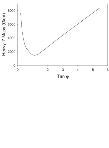
Figure 1: Restriction Curve for $\frac{\epsilon_{1}}{\epsilon_{2}}=1$. The region above the curve gives allowed values of the parameters, while the region below the curve is phenomenologically excluded.

In this model, the value of $R_{b}$ can be greater or less than the SM value, so there is the possibility that this model can explain the $1.8\sigma$ deviation in the experimental value of $R_{b}$ from the SM value. We have that

$$\frac{\delta R_{b}}{R_{b}}=0.8456\cos^{2}\phi\frac{\epsilon_{1}\sin^{2}\phi-\epsilon_{2}\cos^{2}\phi}{(g_{V}^{b})^{2}+(g_{A}^{b})^{2}}$$ (4)

where $\delta R_{b}$ is the Topflavor model value of $R_{b}$ minus the SM value. Thus the direction $R_{b}$ goes in this model depends on the interplay of $\epsilon_{1}$ and $\epsilon_{2}$ tempered by $\phi$. The recent value of $R_{b}$, $0.2178\pm 0.0011$, can be accommodated to within $1\sigma$. For example, with $\frac{\epsilon_{1}}{\epsilon_{2}}=3$, $\tan\phi=0.9$, and $M_{Z_{h}}=1400$ GeV, $R_{b}$ is 0.2169. This model provides no explanation for the $A_{FB}^{\circ,\tau}$ anomaly.[4]

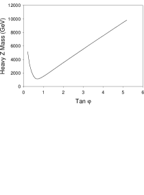
Figure 2: Restriction Curve for $\frac{\epsilon_{1}}{\epsilon_{2}}=3$.

4 Processes at Future Colliders

We now consider the potential of future colliders to detect phenomenology particular to this model. The best chance of observing the heavy $W$ boson is at a high energy hadronic collider such as the LHC. The optimum condition for producing $W_{h}$ in such a fashion is when $\tan\phi$ is large since the coupling of the first generation fermions to the $W_{h}$ goes as $\tan\phi$ and hence the production rate goes as $\tan^{2}\phi$. The cross section for the production of the $W_{h}$ at the LHC with $\sqrt{s}=14$ TeV is shown in Fig. 3. The curve takes $\frac{\epsilon_{1}}{\epsilon_{2}}=1$, but the results are very similar for other values of that ratio. As the figure shows, the value of the cross section can be quite large for smaller values of allowed mass: for example with $\tan\phi=1$ and $M_{W_{h}}=2$ TeV, the cross section is about 3 nb. Thus, if the heavy $W$ boson has a mass in the few TeV range, it will be within the discovery reach of the LHC.

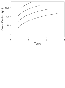
Figure 3: Heavy $W$ Production at the LHC. From top to bottom, the curves are for $M_{W_{h}}$ = 2000, 3000, 4000, and 5000 GeV.

At the LHC there is also the potential for single top production through the production of a heavy $W$ boson and its subsequent decay to a top and bottom quark. For allowed values of the parameters and a heavy $W$ mass in the few TeV range, the cross section for this process typically ranges between a tenth to a half of what it is for top pair production through gluon fusion. For example, for $\tan\phi=1$ and $M_{W_{h}}=2000$ GeV, the cross section is 0.44 nb. A distinctive signature of this process is 2 b-jets plus a single large $p_{\rm T}$ charged lepton.

A process of considerable current interest is $e^{+}e^{-}\rightarrow W_{l}^{+}W_{l}^{-}$ which will provide an important test of the SM prediction for the tri-gauge coupling of the $W$ to the $Z$. Unfortunately, the Topflavor prediction for the $W_{l}$ pair production cross section at LEP-II is not significantly different from the SM value for allowed values of the $Z_{h}$ mass. This is largely due to the fact that the coupling of $W_{l}$ to $Z_{h}$ vanishes to zeroth order in the $\epsilon_{1}$ and $\epsilon_{2}$.

In the Topflavor model, the process $e^{+}e^{-}\rightarrow\mu^{+}\mu^{-}$ gets extra contributions from $Z_{h}$ exchange. Since the $Z_{h}$ mass has to be greater than a TeV, the deviation in the predicted cross section from the SM value is insignificant for LEP-II energies. At the NLC, however, the difference in the predictions for the cross section is significant.

5 FCNC effects

This theory contains FCNC interactions at tree level since the couplings of the third family’s left-handed fermions to the $Z$’s differ from those of the first and second families. The part of the Lagrangian that contains the FCNC interactions is

$${\cal L}^{off-diag}_{neutral}=\overline{U}_{L}\gamma^{\mu}X_{L}^{\dagger}[d_{l}^{(u)}Z_{l,\mu}+d_{h}^{(u)}Z_{h,\mu}]X_{L}U_{L}$$

$$+\ \overline{D}_{L}\gamma^{\mu}Y_{L}^{\dagger}[d_{l}^{(d)}Z_{l,\mu}+d_{h}^{(d)}Z_{h,\mu}]Y_{L}D_{L}$$ (5)

where $U_{L}\equiv(u,c,t)_{L}$ and $D_{L}\equiv(d,s,b)_{L}$. Only the (3,3) elements of the four matrices $d_{l}^{(u)}$, $d_{h}^{(u)}$, $d_{l}^{(d)}$, and $d_{h}^{(d)}$ are nonzero and these are given in terms of $\epsilon_{1}$, $\epsilon_{2}$, and $\phi$. Moreover, $X_{L}$ and $Y_{L}$ relate the gauge to the mass eigenstates of the up and down sectors, respectively. Since $X_{L}$ and $Y_{L}$ are related to the CKM matrix, $K$, by $K=X_{L}^{\dagger}Y_{L}$, we can use the CKM matrix to eliminate $X_{L}$ from Eq. 5. Then using the observed hierarchy of the CKM matrix, $K_{ii}\simeq 1>>K_{ij}$ for $i\not=j$, we can relate the FCNC couplings in the up and down sectors. For example, the part of the Lagrangian involving $Z_{l}$ with the top and charm quarks can be written as

$$\{\overline{c}_{L}\gamma^{\mu}[(d^{(u)}_{l})_{33}(Y_{L}^{\dagger})_{23}(Y_{L})_{33}]t_{L}+h.c.\}Z_{l,\mu}\ ,$$

while that involving $Z_{l}$ with the strange and bottom quarks is

$$\{\overline{s}_{L}\gamma^{\mu}[(d^{(d)}_{l})_{33}(Y_{L}^{\dagger})_{23}(Y_{L})_{33}]b_{L}+h.c.\}Z_{l,\mu}\ .$$ (6)

We get similar expressions involving $Z_{h}$. These contain the same factor of $(Y_{L}^{\dagger})_{23}(Y_{L})_{33}$, thus the FCNC interactions involving $b\overline{s}$ will constrain those involving $t\overline{c}$.

As an example, we can use the limit on the the branching fraction $B(B_{s}^{\circ}\rightarrow\mu^{+}\mu^{-})<8.4\times 10^{-6}$ set by the CDF collaboration [6] to obtain an upper limit on single top production at an NLC type collider. For example, taking $\tan\phi=1.0$, $M_{Z_{h}}=2.2$ TeV, $\sqrt{s}=1$ TeV, and $B(B_{s}^{\circ}\rightarrow\mu^{+}\mu^{-})\sim 10^{-6}$ gives $\sigma(e^{+}e^{-}\rightarrow t\overline{c})=0.2$ pb. One distinctive signature of this process is a single b-jet and a large $p_{\rm T}$ lepton coming from the decay of the top.

6 Conclusion

The model presented here has extra, essentially degenerate, charged and neutral gauge bosons which give rise to interesting phenomenology. Analysis of the existing data allow the extra gauge bosons to have mass as low as about a TeV and as low as a few TeV for a wide range of the mixing angle $\phi$. The experimental value of $R_{b}$ can be accommodated. Future colliders such as the LHC will be able to observe these gauge bosons directly or indirectly if the mass is in the few TeV range. The model gives rise to single top production at both hadronic and leptonic colliders with clear signatures. There is the potential for FCNC interactions with observable rates.

Since one of the weak SU(2)’s can be stronger than SU(2)_W, this model can have baryon number violation via an instanton channel ala ’t Hooft.[7] This will further restrict the allowed parameter space in $\phi$. These and other details of the model will be presented elsewhere.[8]

References

References

- [1] C. T. Hill, Phys. Lett. B 266, 419 (1991); ibid., B 345, 483 (1995); C. T. Hill and S. J. Parke, Phys. Rev. D 49, 4454 (1994).
- [2] X. Li and E. Ma, Phys. Rev. Lett. 47, 1788 (1981); ibid., 60, 495 (1988); Phys. Rev. D 46, R1905 (1992); J. Phys. G 19, 1265 (1993); R. S. Chivukula, E. H. Simmons, and J. Terning, Phys. Lett. B 331, 383 (1994); ibid., Phys. Rev. D 53, 5258 (1996); E. Malkawi, T. Tait, and C. P. Yuan, hep-ph/9603349.
- [3] A preliminary investigation of the Topflavor model with only one Higgs doublet can be found in D. J. Muller and S. Nandi, hep-ph/9602390, to be published in Phys. Lett. B; see also E. Malkawi, T. Tait, and C. P. Yuan, hep-ph/9603349.
- [4] See A. Blondel, talk at this conference; Combination of ALEPH, DELPHI, L3, SLD, and OPAL results, quoted by Paul Langacker and Marcel Demarteau at the 1996 meeting of the Division of Particles and Fields, Minneapolis, MN.
- [5] Particle Data Group, R. M. Barnett et al., Phys. Rev. D54 (1996).
- [6] CDF Colaboration, F. Abe et al., Phys. Rev. Lett. 76, 4675 (1996).
- [7] G. ’t Hooft, Phys. Rev. Lett. 37, 8 (1976); ibid., Phys. Rev. D 14, 3432 (1976).
- [8] D. J. Muller and S. Nandi (in preparation).