Lattice study of classical inflaton decay

Abstract

We study numerically the decay of the inflaton by solving the full non-linear equations of motion on the lattice. We confirm that parametric resonance is effective in transferring energy from the inflaton to a scalar field as long as the self-interactions of the second field are very small. However, in the very broad resonance case ($q\gg 1$) the decay rate is limited by scatterings, which significantly slows down the decay. We also find that the inflaton cannot decay via parametric resonance into a scalar field with moderate self-interactions. This means that the preheating stage may be completely absent in many natural inflationary models.

I Introduction

According to inflationary scenarios of cosmic evolution the Universe undergoes a period of exponential expansion after which it is essentially devoid of matter. At this stage the energy density is almost entirely in the large oscillating expectation value (EV) of the scalar field that drives inflation, the inflaton. The theory of reheating is concerned with the question how this energy is transferred from the inflaton to other fields and eventually thermalized. Early calculations assumed that the inflaton would decay to lighter particles via perturbative decay [1]. It was only recently realized [2] that non-perturbative mechanisms may completely dominate the reheating process. In particular the classical phenomenon of parametric resonance may lead to explosive particle production and very rapid decay of the inflaton field [3]. This stage of the evolution, called preheating in the literature, leads to very different physics than would be obtained from slow perturbative decay. Different aspects have been investigated by many authors [4].

In this paper we present the first fully non-linear study of inflaton decay into a second scalar field. By fully non-linear we mean that we take into account the back reaction of the created particles on the equations of motion as well as their scattering. This is accomplished by integrating the classical equations of motion of the system with certain random initial conditions, a technique that was first applied to the one field case in [5]. The system is modeled by a simple two scalar theory with effective potential

$$V(\phi,\chi)=\frac{1}{2}m^{2}\phi^{2}+\frac{1}{2}\mu^{2}\chi^{2}+\frac{\lambda_{\phi}}{4}\phi^{4}+\frac{\lambda_{\chi}}{4}\chi^{4}+\frac{g}{2}\phi^{2}\chi^{2}.$$ (1)

We will focus on two general classes of inflaton potentials $V(\phi)$: type I for which $\phi\ll m/\sqrt{\lambda_{\phi}}$ (for these we will set $\lambda_{\phi}=0$), and type II for which $\phi\gg m/\sqrt{\lambda}_{\phi}$ (for these we will set $m=0$). In both cases we will assume that there is a channel for the inflaton to decay into a light scalar and thus set the tree level mass $\mu$ of the $\chi$-field to zero. The effects of a massive decay product have been investigated using the Hartree approximation in [6]. For type I models we will neglect the expansion of the Universe[7]. For type II models our calculations are directly applicable to the expanding Universe, as will be explained in section IV.

With the above approximations and neglecting $\lambda_{\chi}$ the equations of motion for the modes of the $\chi$-field are

$$\frac{d^{2}\chi_{k}}{dt^{2}}+(k^{2}+g\phi^{2}(t))\chi_{k}=0\,.$$ (2)

For type I models, where the oscillations of the $\phi$-field EV are sinusoidal, this can be written as the Mathieu equation

$$\frac{d^{2}\chi_{k}}{dz^{2}}+(A(k)-2q\cos(2z))\chi_{k}=0\,,$$ (3)

where $z=\omega_{\phi}t$, $A(k)=k^{2}/\omega_{\phi}^{2}+2q$, $q=g\Phi^{2}/4\omega_{\phi}^{2}$, $\omega_{\phi}=m$ is the frequency of the oscillations, and $\Phi$ is the slowly varying amplitude of the inflaton EV. For type II models the oscillations of $\phi$ are given by elliptic functions, but for the illustrative purpose at hand it is sufficient to replace the periodic EV by a sinusoid of the same frequency. In that case the $\chi$ modes again satisfy (3), except that now $\omega_{\phi}=c\sqrt{\lambda}_{\phi}\Phi$, where $c\approx 0.85$. The important point is that (3) has exponentially growing solutions of the form $\chi_{k}\propto\exp(\mu^{(n)}_{k}z)$ within a set of resonance bands labeled by the integer index n. This growth of the modes corresponds to exponentially growing occupation numbers $n_{k}\propto\exp(2\mu^{(n)}_{k}\omega_{\phi}t)$ and may be interpreted as particle creation. Parenthetically we remark that for type II models the inflaton may also decay into its own fluctuations. Writing $\phi=\langle\phi\rangle+\delta\phi$ and linearizing one finds that the $\delta\phi_{k}$ also (approximately) obey (3), with $A\approx k^{2}/\omega_{\phi}^{2}+2.08$ and $q\approx 1.04$. For $g\gg\lambda_{\phi}$ the decay into $\chi$-fluctuations dominates, however, because the relevant values of $\mu^{(n)}_{k}$ are a few times larger.

The literature distinguishes between narrow resonance, defined by $q\ll 1$, and broad resonance, for which $q\gtrsim 1$. While the first case can be analyzed analytically [8], it is more difficult to obtain quantitative results for the broad resonance case [3]. It is precisely this regime, however, which is most interesting: models generally have $q\gg 1$ at the end of inflation, and it is broad resonance that leads to explosive particle creation. To get a feel for the values of the parameters involved, note that typically $\Phi_{0}\sim M_{\rm P}$ at the end of inflation, where $M_{\rm P}=1/\sqrt{8\pi G}=2.4\times 10^{18}$ GeV is the reduced Planck mass. COBE data [9] restrict $m\lesssim 10^{-6}M_{\rm P}$ for type I models and $\lambda_{\phi}\lesssim 10^{-12}$ for type II models. To prevent radiative corrections from generating an inflaton self-coupling in conflict with COBE, one generally needs $g^{2}\lesssim\lambda_{\phi}|_{max}$, i.e. $g\lesssim 10^{-6}$. Finally, if $\chi$ is to represent a “standard” field then there is no reason for its self-interaction (as well as its coupling to other fields) to be tiny. Thus one might expect $\lambda_{\chi}\sim 10^{-2}-1$. The upshot of all this is that there is a “natural” hierarchy for the couplings in the model,

$$\lambda_{\chi}\gg g\gg\lambda_{\phi}\,,$$ (4)

and that q is generally large at the end of inflation. We believe that the role of $\lambda_{\chi}$ is of particular importance, especially since the final state self-coupling has been ignored in much of the literature so far. The exception is reference [10], where it is was found that the self-interactions can have important effects in the case of narrow resonance. Below we will see that the same holds true in the physically important broad resonance regime.

The difficulty in analyzing the broad resonance case stems from the fact that all parameters in the Mathieu equation for the modes vary quite rapidly. For q very large particle production takes place during a tiny fraction of the period as the EV passes through zero. The amplitude $\Phi$ of the oscillations decreases as energy is transferred from the zero mode to the fluctuations. The produced $\chi$ particles generate a contribution to the mass of the inflaton of the form $g\langle\chi^{2}\rangle$, which changes $\omega_{\phi}$. The $\chi$-field self-interaction, which we ignored in deriving the Mathieu equation for the fluctuations, produces an effective $\chi$ mass of the form $m^{2}_{\chi,\rm eff}\approx 3\lambda_{\chi}\langle\chi^{2}\rangle$. This adds to $A(k)$ the time dependent term $m^{2}_{\chi,\rm eff}/\omega_{\phi}^{2}$. In addition to these backreaction effects there is scattering: the resonance produces particles in narrow momentum bins with large occupation numbers, and one certainly expects these to scatter and spread out rapidly. This effect turns out to be very important, and it has not previously been studied in two field models.

II The method

In order to take all of the above into account quantitatively we discretized the exact classical equations of motion and solved them on a three dimensional lattice. The classical equations of motion are a good approximation to the dynamics provided the mode amplitudes are large in the sense that the commutator of the canonical variables can be replaced by the Poisson brackets, which reduces to $\phi_{k}\dot{\phi}_{k}\gg 1$ [5, 11]. Although our initial state, which will be described below, does not satisfy this condition, it is satisfied very soon after the resonant decay begins. It is useful for the numerics to work in terms of dimensionless variables. We use $\tilde{x}_{\mu}=\sqrt{g}\Phi_{0}x_{\mu}$, $\tilde{m}=m/\sqrt{g}\Phi_{0}$, $\tilde{\lambda}_{\phi}=\lambda_{\phi}/g$, $\tilde{\lambda}_{\chi}=\lambda_{\chi}/g$, $\tilde{\phi}=\phi/\Phi_{0}$, and $\tilde{\chi}=\chi/\Phi_{0}$. In terms of these variables the initial inflaton EV amplitude $\Phi_{0}$ as well as $g$ completely disappear from the equations of motion. While $\Phi_{0}$ simply sets the scale in the problem and becomes irrelevant for the dynamics, the coupling $g$ is still important: it appears in the equations for the random initial fluctuations and regulates their amplitude compared to the EV. The fields are evolved using an explicit algorithm which is second order accurate in time and fourth order accurate in space. We varied both the number of grid points and the lattice spacing to check that we are near the continuum limit. The data presented in this paper were obtained on $128^{3}$ lattices. Regarding numerical accuracy we note that the total energy of the two field system was conserved to better than $1\%$ in all of our runs.

The initial conditions for the numerical simulation were chosen according to the following reasoning: the initial amplitude of the inflaton field is naturally of order the reduced Planck mass, $\Phi_{0}\sim M_{\rm P}\equiv 1/\sqrt{8\pi G}=2.4\times 10^{18}$GeV[12]. Typical values of the resonant momenta are given by $A-2q\sim\sqrt{q}$, which leads to

$$k_{\rm res}\sim\left(\frac{\omega_{\phi}\sqrt{g}\Phi_{0}}{2}\right)^{1\over 2}\simeq\left(\frac{\sqrt{g}\Phi_{0}}{\omega_{\phi}}\right)^{1\over 2}\frac{2M_{\rm P}}{\Phi_{0}}H\simeq q^{1\over 4}\frac{2M_{\rm P}}{\Phi_{0}}H\,.$$ (5)

For $q\gg 1$ this implies that $k_{\rm res}/H\gg 1$ at the end of inflation. Since this ratio does not decrease at later times, the resonant momenta are always on subhorizon scales. These momenta are not squeezed by inflation, and to a good approximation they are zero point quantum fluctuations. The initial conditions may then be approximated by a set of harmonic oscillators in the ground state. We define the phase space in terms of mode amplitudes $\{\chi_{k},\dot{\chi}_{k}\}$ for which $\langle\chi_{k}\rangle=\langle\dot{\chi}_{k}\rangle=0$. These are defined as the minimum uncertainty states with $\langle|\chi_{k}|^{2}\rangle=1/(2\omega_{k})$ and $\langle|\dot{\chi}_{k}|^{2}\rangle=\omega_{k}/2$, where $\omega_{k}$ is the appropriate mode frequency. In the semiclassical approximation these states are populated according to the phase space probability distribution. In our code we randomly generate gaussian distributed states with the width given by $(2\omega_{k})^{-1/2}$ for $\chi_{k}$ and $(\omega_{k}/2)^{1/2}$ for $\dot{\chi}_{k}$, and similarly for the $\phi$ modes. We point out that the evolution does not depend on details of the initial conditions, as long as the initial field configurations have the correct amplitudes [13].

III Massive inflaton (Type I models)

A Models with $\lambda_{\chi}=0$

Let us begin by discussing the simplest possible situation, namely a type I model with $\lambda_{\chi}=0$. For the run presented here the parameters were chosen as follows: $g=10^{-8}$, $m^{2}=10^{-12}\Phi_{0}^{2}$, and lattice spacing $\Delta x=5\pi/4$. The initial amplitude of the $\phi$-field EV, $\Phi_{0}$, sets the scale and does not effect the dynamics in any way, as discussed above. Note that for these values the q parameter in the Mathieu equation is $q=2500$, putting us in the broad resonance regime.

Figure 1 shows the EV of the inflaton field $\phi$, which starts decaying significantly around $t=5000/\sqrt{g}\Phi_{0}=0.5\times 10^{8}\Phi_{0}^{-1}$.

FIG. 1.: The EV of the inflaton as a function of time ($m=10^{-6}\Phi_{0}$, $\lambda_{\chi}=\lambda_{\phi}=0$, $g=10^{-8}$.)

Figure 2 shows the corresponding variances $\langle(\delta\phi)^{2}\rangle=\langle\phi^{2}\rangle-\langle\phi\rangle^{2}$ and $\langle\chi^{2}\rangle$ of the fields.

FIG. 2.: The variances of the fields as a function of time ($m=10^{-6}\Phi_{0}$, $\lambda_{\chi}=\lambda_{\phi}=0$, $g=10^{-8}$).

The variances increase roughly exponentially at first. This trend stops when $\delta m^{2}_{\chi}\equiv g\langle(\delta\phi)^{2}\rangle$ becomes of order the resonant momentum squared. The reason is that the $A(k)$ term in the Mathieu equation gets a contribution of the form $g\langle(\delta\phi)^{2}\rangle/\omega_{\phi}^{2}$. When this term becomes of order $k_{\rm res}^{2}/\omega_{\phi}^{2}$ [14], the resonance band closest to $A=2q$, which has the largest value of $\mu_{k}$, becomes inactive. In the next band $\mu_{k}$ is down by a factor 3 [15] so the decay is slowed down dramatically. The rapid production of inflaton fluctuations, which kills the dominant resonance, may be surprising since there is no $\phi$ resonance in this model. These fluctuations are produced by scatterings of resonant $\chi$-fluctuations off the inflaton EV, which are fast, since both the $\phi$ zero mode and $\chi$ resonant mode amplitudes are large. It is interesting to note that if one analyzes this model using a Hartree type approximation which neglects scattering but includes backreaction effects, then the condition for the end of explosive particle production is that $q(t)\equiv g\Phi(t)^{2}/4(\omega_{\phi}^{2}+g\langle\chi^{2}\rangle)$ becomes $\ll 1$. We emphasize that this is not the correct criterion: our simulations show that scatterings terminate the exponential stage long before $q(t)\lesssim 1$. For example, one sees from figures 2 and 3 that $q(t)\sim 600$ even at $t=5\times 10^{8}\Phi_{0}^{-1}$.

FIG. 3.: The energy densities of the fields as a function of time ($m=10^{-6}\Phi_{0}$, $\lambda_{\chi}=\lambda_{\phi}=0$, $g=10^{-8}$.)

The energy densities of the fields, as well as the total energy density of the system, is shown in figure 3. In the range $t\in[0.8,5]\times 10^{8}\Phi_{0}^{-1}$ the $\chi-$field energy grows like $t^{\alpha}$, with $\alpha\approx 0.95$ and a decay time scale of order $\tau_{\rm decay}\sim 10^{9}\Phi_{0}^{-1}$. Based just on the Mathieu equation one would expect in this range exponential decay with time scale $\tau_{\rm decay}\sim 1/(2\langle\mu_{k}\rangle\omega_{\phi})\sim 10^{7}\,\Phi_{0}^{-1}$. The reason is that as $\Phi$ decays, the resonances sweep through the momentum space, and as they move to higher momenta, $\mu_{k}$ diminishes, and new ones emerge in the infrared (IR). In estimating the above time scale, we have taken the typical value for $\langle\mu_{k}\rangle\sim 0.05$.

To understand why the actual time scale is much longer it is useful to look at the spectrum of fluctuations in k-space. To this end we define “occupation numbers” for the $\chi-$field via

$$n_{k}^{\chi}=\frac{\omega^{\chi}_{k}}{2}\langle\chi_{\vec{k}}\chi_{-\vec{k}}\rangle+\frac{1}{2\omega_{k}^{\chi}}\langle\dot{\chi}_{\vec{k}}\dot{\chi}_{-\vec{k}}\rangle\,,$$ (6)

where $\omega^{\chi}_{k}=\sqrt{k^{2}+g\langle\phi^{2}\rangle}$, and the brackets denote averaging over directions. The $n_{k}^{\phi}$ are defined similarly, except that $\omega^{\phi}_{k}=\sqrt{k^{2}+m^{2}+g\langle\chi^{2}\rangle}$. Figure 4 shows the occupation numbers of the $\chi$-field at various times.

FIG. 4.: $\chi$-field occupation numbers vs. momentum at early times. Three resonances are visible ($t^{*}=\sqrt{g}\Phi_{0}t$).

The growth is exponential at first, with the lowest three resonance bands clearly visible at $k\approx.025$, $k\approx.09$, and $k\approx.13$, respectively. The values of $\mu_{k}^{(n)}$ obtained by assuming $n_{k}^{\chi}\propto\exp 2\mu_{k}^{(n)}\omega_{\phi}t$ agree well with the predictions from the Mathieu equation. For the last time shown in figure 4, scatterings are already becoming important, and the resonance peaks get smeared out.

The subsequent evolution is shown in figure 5.

FIG. 5.: $\chi$-field occupation numbers vs. momentum at later times, when scatterings dominate ($t^{*}=\sqrt{g}\Phi_{0}t$).

Scatterings are very fast after $t\approx 0.5\times 10^{8}\Phi_{0}^{-1}$, and the resonant peak structure is quickly washed out. The occupation numbers grow to about $n^{\chi}_{k}\sim 1/g$, and then remain approximately constant. There is a simple feedback mechanism which explains this behavior. Resonant particle production increases $n^{\chi}_{k_{\rm res}}$, which increases the scatterings off the zero mode, which increases infrared $\phi$ occupation numbers. This increases $\delta m_{\chi}^{2}\equiv g\langle(\delta\phi)^{2}\rangle$, which decreases $\mu_{k}$ (cf. [15]), slowing down resonant particle production and giving scatterings time to move particles toward higher momenta. This reduces $\langle(\delta\phi)^{2}\rangle$, which increases $\mu_{k}$, increasing resonant production and completing the feedback mechanism. Consequently $n_{k_{\rm res}}^{\chi}$ reaches an equilibrium value for which on average scatterings remove particles from the resonance as quickly as they are created, implying $\dot{\rho}_{\rm res}^{\chi}/\rho_{\rm res}^{\chi}=2\mu_{k}\omega_{\phi}-\Gamma_{\rm scatt}\sim 0$. The result is a slowly varying distribution with a characteristic shape, as seen at late times in figure 5. The slope $-k\,d\ln n^{\chi}_{k}/dk$ is small ($\lesssim 2$) in the infrared, grows as $k$ increases, and eventually becomes greater than $4$ at the scale $\Lambda$ at which most of the $\chi$ energy is concentrated. Particles created by the resonance diffuse to this scale $\Lambda$ via scatterings and slowly move it to higher momentum. (Note that soon after scatterings become fast, $\Lambda\gg k_{\rm res}$.) Since the IR occupation numbers of the fields remain roughly constant during this process, the energy required is supplied by the zero mode. The number of $\phi$ zero mode “particles” eaten up in moving one $\chi$ particle from $k_{\rm res}$ to $\Lambda$ is about $N^{\phi}_{0}\sim\Lambda/\omega_{\phi}\gg 1$, implying that scatterings are responsible for most of the EV decay. The upshot is that energy is drained from the zero mode at a slowly varying rate given by $\dot{\rho_{\phi}}\sim N^{\phi}_{0}\rho^{\chi}_{\rm res}\,2\mu_{k}\omega_{\phi}$, where $\rho^{\chi}_{\rm res}$ is the energy density in the $\chi$ resonance. This implies a decay time scale

$$\tau_{\rm decay}\sim\frac{\rho_{\phi}}{\dot{\rho_{\phi}}}\sim\frac{\rho_{\phi}}{\rho_{\rm res}^{\chi}\,2\mu_{k}\omega_{\phi}}\frac{\omega_{\phi}}{\Lambda}\sim\frac{3\times 10^{3}}{gn_{k_{\rm res}}^{\chi}}\frac{\omega_{\phi}}{\Lambda}\frac{1}{\omega_{\phi}}\,.$$ (7)

To obtain the last expression in Eq. (7) we used

$$\rho_{\rm res}^{\chi}\simeq\int_{\rm res}\frac{d^{3}k}{(2\pi)^{3}}n_{k}^{\chi}\omega_{k}^{\chi}\sim\frac{k_{\rm res}^{3}}{2\pi^{2}}w_{\rm res}n_{k_{\rm res}}^{\chi}\,,$$ (8)

where the resonance width $w_{\rm res}$ is approximately given by

$$w_{\rm res}\simeq 0.8k_{\rm res}\exp{[-(m_{\chi}^{2}+k^{2})/(\Delta k)^{2}]}\,,$$ (9)

as well as $k_{\rm res}^{2}$ $\simeq$ $\sqrt{q}\omega_{\phi}^{2}=\sqrt{g}m_{\phi}\Phi/4$, and $\mu_{k}\simeq 0.23\exp{[-(m_{\chi}^{2}+k^{2})/(\Delta k)^{2}]}$. Here $\Delta k\simeq(\sqrt{g}m_{\phi}\Phi/2)^{1/2}$ denotes the distance between the first two resonances. The numerical coefficient is obtained by noting that resonant energy production peaks around $k\simeq k_{\rm res}$, and $m^{2}_{\chi}\equiv g\langle(\delta\phi)^{2}\rangle\sim k_{\rm res}^{2}$. The last relation remains reasonably well satisfied throughout the scattering regime. This is not surprising, since from $2\mu_{k}\omega_{\phi}\sim\Gamma_{\rm scatt}$ one finds $m_{\chi}^{2}\sim k_{\rm res}^{2}\ln(\Gamma_{\rm scatt}/2\mu_{0}\omega_{\phi})$, i.e. $m_{\chi}^{2}$ is only logarithmically dependent on slowly varying quantities (from above, $\mu_{0}\simeq 0.2/e$). The quantities entering Eq. (7) vary slowly during the scattering dominated regime, and one should take their typical values to get an order of magnitude estimate for the decay time. From figure 5 one reads off $gn_{k_{\rm res}}^{\chi}\simeq 0.04$ and $\Lambda/\omega_{\phi}\sim 70$, which leads to $\tau_{\rm decay}\sim 10^{9}\Phi_{0}^{-1}$. This agrees with the decay time scale seen in figures 1 and 3. The time scale in (7) is naively parametrically larger by $\sim 1/[g\ln(1/g)]$ in comparison to the scale of parametric resonant decay. The reason why the decay time is not huge even for $g$ very small is that $gn^{\chi}_{k_{\rm res}}\sim 0.04$, i.e., the occupation numbers are very large. This however is not true when there is a moderate self-coupling of the $\chi$ field, as will be discussed in section III B.

From the discussion above it is clear that the inflaton decay consists of two distinct regimes: fast exponential decay during which scatterings are irrelevant followed by a much slower decay governed by scattering processes. One can clearly separate these two regimes in figure 2: the scattering regime sets in at the time when the variances become slowly varying, which occurs at $t\simeq 0.8\times 10^{8}\Phi_{0}^{-1}$. Clearly there is a brief transition stage between the two regimes, and since the exponential decay is a stimulated process, this is where most of the energy loss associated with the exponential regime occurs. The resonant occupation numbers stay roughly constant during this transition stage since the scatterings are already fast, but the infrared and near ultraviolet states are quickly filled. One can estimate quite generally what fraction of the inflaton energy has decayed at the time when the slowly varying state sets in, as follows. We have run our code for several values of $g$ in the range $g=10^{-12}$ to $10^{-8}$ and find that $g\langle\chi^{2}\rangle\simeq g\int[d^{3}k/(2\pi)^{3}\omega^{\chi}_{k}]n^{\chi}_{k}\sim\omega_{\phi}^{2}/4$ when the scattering regime begins [16]. This value is somewhat dependent on the exact initial position of the dominant resonance. Since at this time the variance is dominated by modes with $k^{2}\sim\sqrt{g}\omega_{\phi}\Phi_{0}$, we can estimate the occupation numbers of the $\chi$ field around the resonant momentum to be $gn^{\chi}_{k_{\rm res}}\sim 5\omega_{\phi}/\sqrt{g}\Phi_{0}$. At this time the $\chi$ energy is dominated by approximately the same scale $(\sqrt{g}\omega_{\phi}\Phi_{0})^{1/2}$, implying $\rho_{\chi}/(\rho_{\phi})_{0}\sim\omega_{\phi}/\sqrt{g}\Phi_{0}=(1/2){q}^{-1/2}$. This means that for $q\gg 1$ only a small fraction of the inflaton energy decays during the exponential regime [17].

After the scatterings become important, the distribution broadens significantly, but the occupation number at the resonant scale remains to a good approximation constant. With our above estimate for $gn^{\chi}_{k_{\rm res}}$ we can thus give a parametric expression for the decay time in the scattering regime based on Eq. (7). Our numerical results indicate that occupation numbers drop approximately exponentially between $k_{\rm res}$ and $\Lambda$ (cf. figure 5). We take $n_{k}^{\chi}=n_{k_{\rm res}}^{\chi}\exp{[-(k-k_{\rm res})/\kappa]}$, where $1/\kappa$ is the slope of $\ln n_{k}^{\chi}$. As can be seen in figure 5, this value decreases slowly as the field decays. The relevant value of $\kappa$ can be computed by noting that when the EV decays significantly, about half of the original energy density $(\rho_{\phi})_{0}=\omega_{\phi}^{2}\Phi_{0}^{2}/2$ is in the $\chi$ fluctuations. This gives $\kappa^{2}\simeq q^{1/4}\sqrt{g}\Phi_{0}\omega_{\phi}/2$. The scale $\Lambda$ can be evaluated as $\Lambda=\langle k\rangle\simeq 4\kappa$. Combining these results with Eq. (7) we arrive at the following parametric estimate for the decay time (recall that this is sensible only for $q\gg 1$, since otherwise most of the field decays during the exponential regime):

$$\tau_{\rm decay}\sim 3\times 10^{2}q^{\frac{1}{8}}\frac{1}{\omega_{\phi}}\,,\qquad q\gg 1$$ (10)

The main point of this equation is that the decay time is very weakly dependent on $q$. (This conclusion is independent of our assumption that $n_{k}^{\chi}$ falls off exponentially in the relevant momentum range, even though the exact power of $q$ is not.) Note that surprisingly, for fixed $\omega_{\phi}$ and $\Phi_{0}$, the decay time actually slowly increases as $g$ increases. That $\tau_{\rm decay}$ is nearly independent of $q$ in the scattering regime agrees well with our numerical simulations for $2.5\times 10^{3}>q>25$. We have not verified this dependence for much larger values of $q$ because such simulations require enormous computing times. We showed above that the fraction of energy that decays in the exponential regime is $\sim 1/\sqrt{q}\propto 1/\sqrt{g}$, implying that paradoxically the field decays faster for smaller values of $q\propto g$. Our numerical calculations indeed indicate that the fastest inflaton decay occurs for $q\sim 1$, rather than for $q\gg 1$. One should note, however, that in an expanding universe parametric resonance is ineffective for $q\sim 1$ in type I models since the effective $q_{t}$ becomes much less that unity before the resonant occupation numbers grow large [6].

B Models with $\lambda_{\chi}\gg g$

We now investigate what happens when $\lambda_{\chi}\gg g$. As discussed in the introduction, this occurs naturally in many models. For the run to be presented we used $m^{2}=10^{-12}\Phi_{0}^{2}$, $g=10^{-8}$, $\lambda_{\phi}=0$, $\lambda_{\chi}=0.01$, and $\Delta x=5\pi/2$. The evolution in this case is very different from the $\lambda_{\chi}=0$ case (case I$(a)$) considered above. As can be seen from figure 6, the resonance starts growing just as in case I$(a)$.

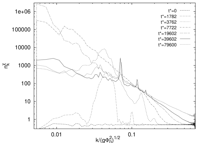
FIG. 6.: $\chi$-field occupation numbers at various times for a model with moderate self-coupling $\lambda_{\chi}=10^{-2}$ ($m=10^{-6}\Phi_{0}$, $\lambda_{\phi}=0$, $g=10^{-8}$ and $t^{*}=\sqrt{g}\Phi_{0}t$).

However, when the occupation numbers reach about $10^{2}/\lambda_{\chi}$, scatterings become fast and populate the infrared states. This gives rise to the backreaction $\delta m^{2}_{\chi}=3\lambda_{\chi}\langle\chi^{2}\rangle$, which shifts the resonances toward the infrared. As the first resonance sweeps through the infrared, it further populates the states. Once the resonance reaches $k\sim 0$, it is no longer very effective so that scatterings remove particles from the infrared faster than they are supplied by the resonance. This leads to depletion of the infrared states, which decreases the backreaction a little, increasing the resonance’s effectiveness. This feedback mechanism leads to a state with slowly varying occupation numbers, just as in case I(a). As a consequence, energy is removed from the zero mode at a slowly varying rate, starting at about $t=2.5\times 10^{8}\Phi_{0}^{-1}$. In contrast to case I(a) the $\phi$ field plays no part in keeping the occupation numbers constant: it is the much faster $\chi-\chi$ scatterings which remove particles from the resonant momenta as they are created [18]. Consequently the EV does not get depleted by scatterings, and the rate of energy density loss of the $\phi$-field is simply $\dot{\rho}_{\phi}\simeq-\rho_{\rm res}^{\chi}2\mu_{k}\omega_{\phi}$, which leads to an estimate of the decay time $\tau_{\rm decay}=-\rho_{\phi}/\dot{\rho}_{\phi}\simeq 10\omega_{\phi}\Phi_{0}^{2}/(2\mu_{k}k_{\rm res}^{3}w_{\rm res}n_{k_{\rm res}}^{\chi})$. The parameters can be deduced from our simulation. The relevant resonance in this case is the second one (recall that the first one has been shifted to the infrared) which can be seen at $k\approx 0.07\sqrt{g}\Phi_{0}$ at late times in figure 6. We estimate $k_{\rm res}^{2}\simeq 0.5\sqrt{g}\omega_{\phi}\Phi_{0}$, $\mu_{k_{\rm res}}\simeq 0.03$, the resonance width $w_{\rm res}\simeq 0.05k_{\rm res}$, and $n_{k_{\rm res}}^{\chi}\simeq 15/\lambda_{\chi}$, so that $\tau_{\rm decay}\sim 10^{4}/(gn_{k_{\rm res}}^{\chi}\omega_{\phi})\sim 10^{15}\Phi_{0}^{-1}$. Note that this time scale is parametrically larger than the resonance decay time by $\lambda_{\chi}/g\ln(1/g)$, which is about $10^{5}$ in our case. We point out that $\langle\chi^{2}\rangle$ reaches a maximum value of about $6\times 10^{-9}\Phi_{0}^{2}$ at $t\sim 2\times 10^{8}\Phi_{0}^{-1}$, and by $t=8\times 10^{8}\Phi_{0}^{-1}$ less than $0.0005\%$ of the energy is in the $\chi$ field [19]. The rate of energy density increase is about $\delta\rho_{\chi}/\delta t\sim 4\times 10^{-28}\Phi_{0}^{5}$. A linear extrapolation gives for the decay time $\tau_{\rm decay}\sim\rho_{\phi}/(\delta\rho_{\chi}/\delta t)\sim 10^{16}\Phi_{0}^{-1}$, in rough agreement with our simple model. We emphasize that we do not claim that at very late times the simple feedback mechanism gives a correct picture. The main point of this simulation was to establish that a moderate self-coupling of the $\chi$ field slows down the EV decay by many orders of magnitude. This conclusion remains valid when $\chi$ couples moderately to other fields. The only difference is that $\chi$ now decays into these fields, which in turn induces backreaction on $\chi$. While the details are model dependent, the basic mechanism remains valid, and parametric resonance is rendered ineffective.

IV Massless inflaton (Type II models)

Let us now turn to type II models. These were investigated using the same techniques as above, so rather than present the results in detail we will simply state our conclusions. Before doing so it is worth pointing out that for these models the expanding universe equations of motion are conformally equivalent to those in Minkowski space. By this we mean that in terms of the variables $\tau=\int dt/a(t)$, $\bar{\phi}=\phi a(\tau)/a(0)$, and $\bar{\chi}=\chi a(\tau)/a(0)$, where $a(\tau)$ is the scale factor, the Friedmann-Robertson-Walker (FRW) equations of motion are of exactly the same form as those in ordinary static spacetime [20]. Hence, with the simple replacements above, our numerical calculations for type II models apply directly to an expanding universe.

The main results of our study are as follows.

A Models with $\lambda_{\chi}=0$

If $\lambda_{\chi}=0$, the inflaton decays via parametric resonance in much the same way as it did in case I(a). That is, after a brief period of exponential decay a slowly varying state sets in during which the decay is dominated by scatterings. For example, figure 7 shows the variances of the fields for $m^{2}=0$, $\lambda_{\phi}=10^{-12}$, and $g=10^{-8}$.

FIG. 7.: The variances of the fields as a function of time for a quartic inflaton potential ($m=0$, $\lambda_{\phi}=10^{-12}$, $g=10^{-8}$).

Since in this case $\omega_{\phi}=0.85\sqrt{\lambda_{\phi}}\Phi_{0}$, $q\approx 3500$. The figure indicates that, as in case I(a), the exponential regime ends at $t\sim 0.8\times 10^{8}\Phi_{0}^{-1}$. The maximum values of the variances are again to a good approximation given by $g\langle\chi^{2}\rangle\sim\omega_{\phi}^{2}$ and $g\langle\phi^{2}\rangle\sim\omega_{\phi}\sqrt{g}\Phi_{0}$. The decay time can still be estimated from (7), with the replacement $m_{\phi}\rightarrow\omega_{\phi}\simeq 0.85\sqrt{\lambda}\Phi_{0}$. The slowly varying value of $gn^{\chi}_{\rm{k_{res}}}$ is again about $5\omega_{\phi}/\sqrt{g}\Phi_{0}$, so type I and II models behave very much alike for equal values of the parameters. One difference is that for type II models the inflaton energy decays somewhat faster, since $\mu_{k}$ is larger and in addition there are scatterings via the $\lambda_{\phi}\phi^{4}$ term. For the $\lambda_{\chi}=0$ runs described in this work, the energy decays about $50\%$ faster for the quartic potential. The value of $\mu_{k}$ is about $25\%$ larger for that case.

As discussed at the beginning of this section, the lattice results for type II models can be mapped onto the expanding universe by the appropriate rescaling. To see how this works in practice consider the problem of obtaining the maximum value of $\langle\chi^{2}\rangle$ reached during preheating in the expanding universe. This value is interesting because it quantifies the effective temperature of non-thermal phase transitions [21]. Since for type II models the universe is radiation dominated we can write $a(\tau)/a(0)=1+H_{0}a(0)\tau$, where $\tau$ is the conformal time and $H_{0}=\sqrt{\lambda}_{\phi}\Phi_{0}^{2}/\sqrt{12}M_{\rm P}$ is the Hubble constant at the end of inflation. As discussed at the beginning of section IV, in a Friedmann-Robertson-Walker universe our lattice fields are rescaled by a factor $a(\tau)/a(0)$ and our lattice time is $\tau$. Hence $\langle\chi_{\rm\;FRW}^{2}\rangle=(a(0)/a(\tau))^{2}\langle\chi^{2}\rangle$. Consider, for example, the variances shown in figure 7. Since $\langle\chi^{2}\rangle$ rises rapidly and then becomes slowly varying, $\langle\chi_{\rm\;FRW}^{2}\rangle_{\rm max}$ occurs at the moment when the fast growth terminates. This occurs at $\tau\approx 8000/\sqrt{g}\Phi_{0}=8\times 10^{7}\Phi_{0}^{-1}$ when $\langle\chi^{2}\rangle\approx 6\times 10^{-5}\Phi_{0}^{2}$. Hence we obtain $\langle\chi_{\rm\;FRW}^{2}\rangle_{\rm max}\approx 6\times 10^{-5}\Phi_{0}^{2}/(1+2\times 10^{7}\sqrt{\lambda}_{\phi}\Phi_{0}/M_{\rm P})^{2}\approx 10^{-7}M_{\rm P}^{2}$, where we have used $a(0)=1$ in our units. We can obtain general formulae for the maximum variances of the fields when $q\gg 1$ by recalling that the slowly varying scattering regime sets in when $g\langle(\delta\phi)^{2}\rangle\sim k_{\rm res}^{2}\sim\sqrt{g}\omega_{\phi}\Phi_{0}/2$ and $g\langle\chi^{2}\rangle\sim\omega_{\phi}^{2}/4$, where $\omega_{\phi}\approx 0.85\sqrt{\lambda}_{\phi}\Phi_{0}$. This occurs when $n^{\chi}_{k_{\rm res}}\sim(g\sqrt{q})^{-1}$, i.e. at the time $\tau\sim\ln(1/g\sqrt{q})/2\mu_{k}\omega_{\phi}$. Combining this with our equation for $a(\tau)$ we obtain

$$\langle(\delta\phi_{\rm\;FRW})^{2}\rangle_{max} \sim 0.2\frac{1}{q^{1/2}\ln^{2}(\lambda_{\phi}^{-1}q^{-3/2})}M_{\rm P}^{2}$$ (12)

$$\sim \left(\frac{\lambda_{\phi}}{g}\right)^{1\over 2}\frac{1}{\ln^{2}(\lambda_{\phi}/g^{3})}M_{\rm P}^{2}$$ (13)

and

$$\langle\chi_{\rm\;FRW}^{2}\rangle_{max} \sim 0.06\frac{1}{q\ln^{2}(\lambda_{\phi}^{-1}q^{-3/2})}M_{\rm P}^{2}$$ (15)

$$\sim \left(\frac{\lambda_{\phi}}{g}\right)\frac{1}{\ln^{2}(\lambda_{\phi}/g^{3})}M_{\rm P}^{2}\;,$$ (16)

where $M_{\rm P}\approx 2.4\times 10^{18}$GeV. These results can be considered upper limits for the variances since they were obtained for a massless $\chi$ field and a mass term in the equations of motion only suppresses the resonance [6]. Note that $\langle\chi_{\rm\;FRW}^{2}\rangle_{max}\propto q^{-1}$ (up to logarithms), while Hartree type approximations which neglect scattering predict a $q^{-1/2}$ dependence [3]. That the Hartree approximation may not give the correct $q$ dependence of $\langle\chi^{2}\rangle$ was previously mentioned in [6].

B Models with $\lambda_{\chi}\gg g$

If $\lambda_{\chi}\gg g$, the situation is drastically changed. Just as for type I models the decay into the $\chi$-field is extremely slow. But for type II models the inflaton can decay into its own fluctuations via parametric resonance, as discussed below Eq. (3). This process, which is much slower than decay into $\chi$ fluctuations for $\lambda_{\chi}=0$, becomes dominant for $\lambda_{\chi}\gg g$. In fact the inflaton decays into its own fluctuations as if it were not coupled to the $\chi$-field at all. We have verified this by running the one field case and comparing the results to the two field simulation with the same parameters in the $\phi$ sector. For example, with $m=0$, $\lambda_{\phi}=10^{-12}$, $\lambda_{\chi}=10^{-2}$ and $g=10^{-8}$ we find that $73\%$ of the energy has decayed by $t=8\times 10^{8}\Phi_{0}^{-1}$ and $\langle(\delta\phi)^{2}\rangle_{\rm max}\approx 8\times 10^{-2}\Phi_{0}^{2}$, which agrees very well with the corresponding one field run. We also note that in the two field run $\langle\chi^{2}\rangle$ grows exponentially at first but then reaches a maximum value of about $3\times 10^{-9}\Phi_{0}^{2}$ at $t\sim 0.4\times 10^{8}\Phi_{0}^{-1}$. The details of the one field case are discussed in [5]. One may wonder why the perturbative energy flow via scatterings from $\phi$ to $\chi$ fluctuations is ineffective even after the infrared $\phi$ occupation numbers reach a huge value of order $\lambda_{\phi}^{-1}\gg g^{-1}$. The reason is that due to the backreaction $g\langle\delta\phi^{2}\rangle\;$, $\chi$ fluctuations become massive and $\phi\phi\rightarrow\chi\chi$ scatterings are kinamatically forbidden. (Indeed, taking the above value for $\langle(\delta\phi)^{2}\rangle_{\rm max}$, one finds $m_{\chi}/\omega_{\phi}\sim 30$.)

We point out that it is very difficult to simulate type II models with large q on the lattice. The reason is that the typical resonant momenta for the two fields differ by a factor $k_{\rm res}^{\phi}/k_{\rm res}^{\chi}\sim q^{-1/4}$, making it difficult to run simulations that capture both resonances with sufficient infrared and ultraviolet resolution. Our numerical results on $128^{3}$ lattices were hence obtained in a two step process: we first did preliminary runs, choosing $\Delta x$ optimally for each resonance in turn. This allowed us to determine which one was dominant, namely the $\chi$ resonance for $\lambda_{\chi}=0$ and the $\phi$ resonance for $\lambda_{\chi}\gg g$. We then did extended runs choosing $\Delta x$ just large enough to capture the physics of the dominant resonance, giving us the best possible ultraviolet range for the given situation.

V Conclusion

We have numerically investigated the decay of the inflaton coupled to a massless scalar field. Our main results for both quadratic (type I) and quartic (type II) inflaton potentials are as follows:

1. If the self-coupling of the decay product is small ($\lambda_{\chi}\ll g$) we find two distinct stages of inflaton decay for $q\gtrsim 25$: an exponential regime in which the field decays via parametric resonance, followed by a scattering dominated regime. The fraction of energy which decays by the time the scattering regime begins is of order $q^{-1/2}$. This means that for $q\gg 1$ scatterings are responsible for most of the inflaton decay, and we find that the decay time scale in the scattering regime is significantly longer than the resonance decay time scale.

2. If $\lambda_{\chi}\gg g$ (which is natural for many models) we find that parametric resonance cannot transfer energy to $\chi$. The reason is that scatterings due to the self-interactions limit the maximum occupation numbers of $\chi$, allowing only a tiny fraction of the inflaton energy to be transferred during the resonant stage. In the subsequent scattering dominated regime the transfer of energy is extremely slow, leading to huge decay times for type I models. For type II models the inflaton decays into its own fluctuations, essentially as if it were not coupled to the second field at all. Although these results were obtained in a simple model with two scalar fields, the basic mechanism, and hence our conclusion, remains valid for a realistic model with many mutually interacting fields.

In this work we have studied inflaton decay by integrating the Minkowski space equations of motion. It is an interesting question how our conclusions might change in an expanding universe. For type II models the answer is simple: as explained in section IV, our analysis is directly applicable after the appropriate rescaling. The mapping was made explicit in section IV A, where we obtained upper limits for the variances of the fields in the expanding universe.

For type I models the situation is more complex. The time scale $H^{-1}$ defined by the the expansion rate $H=\sqrt{\rho_{\phi}/3}/M_{\rm P}\lesssim\omega_{\phi}/2$ is much shorter than the scattering decay time scale (see Eq. (10)). Consequently we cannot expect our work for type I models to be a good approximation to the expanding universe case. However, we do expect our conclusion that the inflaton cannot decay into a field with moderate self-interactions to remain valid. First of all, parametric resonance in an expanding universe is suppressed. Second, in the scattering regime the maximum occupation number will remain of order $\lambda_{\chi}^{-1}$, so one expects that the total energy deposited in the $\chi$ field fluctuations remains a tiny fraction of the inflaton energy even in an expanding universe.

- [1] A. A. Starobinskii, in Quantum Gravity, Proceedings of the Second Seminar “Quantum Theory of Gravity” (Moskow, 13 - 15 Oct. 1981), eds. M. A. Markov ad P. C. West (Plenum, New York, 1984), p. 103; A. Dolgov and A. Linde, Phys. Lett. 116B, 329 (1982); L. F. Abbott, E. Farhi, and M. Wise, Phys. Lett. 117B, 29 (1982).
- [2] J. H. Traschen and R. H. Brandenberger, Phys. Rev. D42, 2491 (1990).
- [3] L. Kofman, A. D. Linde and A. A. Starobinskii, Phys. Rev. Lett. 73, 3195 (1994).
- [4] D. Boyanovsky, D. Cormier, H. J. de Vega, R. Holman, A. Singh, M. Srednicki, report No. UCSBTH-96-23, hep-ph/9609527 (1996); D. Boyanovsky, H. J. de Vega, R. Holman, J. F. J. Salgado, report No. PAR-LPTHE-96-32, hep-ph/9608205 (1996), to be published in Phys. Rev. D, and references therein; D. Kaiser, report No. astro-ph/9507108, Phys. Rev. D 53, 1776 (1996). M. Yoshimura, report No. hep-th/9506176, Prog. Theor. Phys. 94, 873 (1995) and references therein; L. A. Kofman, report No. UH-IFA-96-28, astro-ph/9605155 (1996), to appear in Relativistic Astrophysics: A Conference in Honor of Igor Novikov’s 60th Birthday, eds. B. Jones and D. Marković; D. T. Son, report No. hep-ph/9604340, Phys. Rev. D 54, 3745 (1996).
- [5] S. Yu. Khlebnikov and I. I. Tkachev, Phys. Rev. Lett. 77, 219 (1996).
- [6] S. Yu. Khlebnikov and I. I. Tkachev, report No. PURD-TH-96-06, hep-ph/9608458 (1996).
- [7] While the study of these models in Minkowski space is interesting in its own right, one might expect our numerical calculations to be a reasonable first approximation to the expanding case if , i.e. . This inequality is marginally satisfied.
- [8] Y. Shtanov, J. Traschen and R. Brandenberger, Phys. Rev. D51, 5438 (1995).
- [9] B. A. Campbell, S. Davidson, K. A. Olive, Nucl. Phys. B 399, 111 (1993).
- [10] R. Allahverdi and B. A. Campbell, report No. hep-ph/9606463 (1996).
- [11] This condition assumes the following definition of the Fourier transform: .
- [12] The end of inflation is signaled by a breakdown of the slow-roll condition . The relation then leads to for both and .
- [13] Our initial conditions differ from those used in [6] in that our field amplitudes and “velocities” are not correlated. The authors of [6] obtain correlated initial conditions by evolving the developed resonant solution backward in time, while we simply take the initial state to correspond to random zero point fluctuations. We agree with the authors that the details of the initial conditions do not affect the evolution in any significant way, so long as they have the correct amplitudes. We have verified this explicitly by reproducing the results of [5] using our initial conditions.
- [14] The initial position of the dominant resonance depends on the exact value of , and can be anywhere between and , where is the typical distance between the first two resonances.
- [15] We find that for the first few resonances above the maximum decays approximately as , where is the distance between the resonances, and . The width of the resonances is also decreasing exponentially.
- [16] This observation can be understood as follows. At the beginning of the scattering regime the flow of energy between the two fields is fairly efficient since the scatterings are already fast. Thus one might expect that equipartition of energy between and fluctuations is reasonably well satisfied. (We typically find that at this stage the energy in fluctuations is several times larger than that in fluctuations. At later stages equipartition is well satisfied.) From one finds , where we have assumed that the energy in the and fluctuations is concentrated at the scales and , respectively. Recall that the backreaction renders the dominant resonance inactive when , from which one obtains . Combining these estimates, we find and hence .
- [17] One may wonder how this changes in an expanding universe. In terms of the variables and , where , the obey an approximate Mathieu equation, with time dependent parameters and . Since (except very early when it is ), changes slowly and the adiabatic approximation should be reasonably accurate. The scattering regime begins at , which can be used to compute . One may go through a similar resoning as in the Minkowski case presented in the main text, to obtain that the scattering regime is important when . (At this time the fraction of energy in the fluctuations is about .) This leads to the initial value .
- [18] The fact that scatterings of particles off the zero mode are not important in this case can be verified by looking at the field occupation numbers. We find that at all times and for all during our simulation. Similarly, at all times, which may be compared to figure 2.
- [19] One can estimate the energy in the fluctuations at the time when the slowly varying state begins as follows: the scatterings via the term become fast when . The energy density at that time is , so that the fraction of the total energy in fluctuations is about .
- [20] This is true only for , but remains approximately true for sufficiently small. It also requires that the Universe is radiation dominated, as is indeed the case for models with pure potentials [8]. In this case and .
- [21] L. Kofman, A. Linde, A. A. Starobinskii, report No. hep-th/9510119, Phys. Rev. Lett. 76, 1011 (1996); I. I. Tkachev, report No. hep-th/9510146, Phys. Lett. B 376, 35 (1996); A. Riotto, I. I. Tkachev, Phys. Lett. B385, 57 (1996). E. W. Kolb, A. Linde, A. Riotto, report No. FERMILAB-PUB-96-133-A, hep-ph/9606260 (1996); G. W. Anderson, A. Linde, A. Riotto report No. FERMILAB-PUB-96-078-A, hep-ph/9606416 (1996).