CERN-TH/96-292

hep-ph/9610nnn

Heavy-Quark Effective Theory

Matthias Neubert

Theory Division, CERN, CH-1211 Geneva 23, Switzerland

We give an introduction to the heavy-quark effective theory and the $1/m_{Q}$ expansion, which provide the modern framework for a systematic, model-independent description of the properties and decays of hadrons containing a heavy quark. We discuss the applications of these concepts to spectroscopy and to the weak decays of $B$ mesons.

Invited talk presented at the

20th Johns Hopkins Workshop on Current Problems in Particle Theory

Heidelberg, Germany, 27-29 June 1996

CERN-TH/96-292
October 1996

Abstract

We give an introduction to the heavy-quark effective theory and the $1/m_{Q}$ expansion, which provide the modern framework for a systematic, model-independent description of the properties and decays of hadrons containing a heavy quark. We discuss the applications of these concepts to spectroscopy and to the weak decays of $B$ mesons.

1 Introduction

The weak decays of hadrons containing a heavy quark are employed for tests of the Standard Model and measurements of its parameters. They offer the most direct way to determine the weak mixing angles, to test the unitarity of the Cabibbo–Kobayashi–Maskawa (CKM) matrix, and to explore the physics of CP violation. At the same time, hadronic weak decays also serve as a probe of that part of strong-interaction phenomenology which is least understood: the confinement of quarks and gluons inside hadrons.

The structure of weak interactions in the Standard Model is rather simple. Flavour-changing decays are mediated by the coupling of the charged current to the $W$-boson field. At low energies, the charged-current interaction gives rise to local four-fermion couplings, whose strength is governed by the Fermi constant

$$G_{F}={g^{2}\over 4\sqrt{2}M_{W}^{2}}=1.16639(2)~{}\mbox{GeV}^{-2}\,.$$ (1)

According to the structure of the these interactions, the weak decays of hadrons can be divided into three classes: leptonic decays, in which the quarks of the decaying hadron annihilate each other and only leptons appear in the final state; semileptonic decays, in which both leptons and hadrons appear in the final state; and non-leptonic decays, in which the final state consists of hadrons only. Representative examples of these three types of decays are shown in Fig. 1.

Figure 1: Examples of leptonic ($B^{-}\to\tau^{-}\bar{\nu}_{\tau}$), semileptonic ($\bar{B}^{0}\to D^{+}e^{-}\bar{\nu}_{e}$), and non-leptonic ($\bar{B}^{0}\to D^{+}\pi^{-}$) decays of $B$ mesons.

The simple quark-line graphs shown in this figure are a gross oversimplification, however. In the real world, quarks are confined inside hadrons, bound by the exchange of soft gluons. The simplicity of the weak interactions is overshadowed by the complexity of the strong interactions. A complicated interplay between the weak and strong forces characterizes the phenomenology of hadronic weak decays. As an example, a more realistic picture of a non-leptonic decay is shown in Fig. 2. Clearly, the complexity of strong-interaction effects increases with the number of quarks appearing in the final state. Bound-state effects in leptonic decays can be lumped into a single parameter (a “decay constant”), while those in semileptonic decays are described by invariant form factors, depending on the momentum transfer $q^{2}$ between the hadrons. Approximate symmetries of the strong interactions help to constrain the properties of these form factors. For non-leptonic decays, on the other hand, we are still far from having a quantitative understanding of strong-interaction effects even in the simplest decay modes.

Figure 2: More realistic representation of a non-leptonic decay.

Over the last decade, a lot of information on heavy-quark decays has been collected in experiments at $e^{+}e^{-}$ and hadron colliders. This has led to a rather detailed knowledge of the flavour sector of the Standard Model and many of the parameters associated with it. There have been several great discoveries in this field, such as $B^{0}$–$\bar{B}^{0}$ mixing [1, 2], charmless $B$ decays [3]^-[5], and rare decays induced by penguin operators [6, 7]. The experimental progress in heavy-flavour physics has been accompanied by a significant progress in theory, which was related to the discovery of heavy-quark symmetry and the development of the heavy-quark effective theory (HQET). The excitement about these developments is caused by the fact that they allow (some) model-independent predictions in an area in which “progress” in theory often meant nothing more than the construction of a new model, which could be used to estimate some strong-interaction hadronic matrix elements. Here we explain the physical picture behind heavy-quark symmetry and discuss the construction, as well as simple applications, of the heavy-quark expansion. Because of lack of time, we will have to focus on some particularly important aspects. A more complete discussion of the applications of this formalism to heavy-flavour phenomenology can be found in some recent review articles [8]^-[10]. The reader is also encouraged to consult the earlier review papers [11]^-[15] on the subject.

Hadronic bound states of a heavy quark with light constituents (quarks, antiquarks and gluons) are characterized by a large separation of mass scales: the heavy-quark mass $m_{Q}$ is much larger than the mass scale $\Lambda_{\rm QCD}$ associated with the light degrees of freedom. Equivalently, the Compton wave length of the heavy quark ($\lambda_{Q}\sim 1/m_{Q}$) is much smaller than the size of the hadron containing the heavy quark ($R_{\rm had}\sim 1/\Lambda_{\rm QCD}$). Our goal will be to separate the physics associated with these two scales, in such a way that all dependence on the heavy-quark mass becomes explicit. The framework in which to perform this separation is the operator product expansion (OPE) [16, 17]. The HQET provides us with a convenient technical tool to construct the OPE. Before we start to explore the details of this effective theory, however, we should mention two important reasons why it is desirable to separate short- and long-distance physics in the first place:

• A technical reason is that after the separation of short- and long-distance phenomena we can actually calculate a big portion of the relevant physics (i.e. all short-distance effects) using perturbation theory and renormalization-group techniques. In particular, in this way we will be able to control all logarithmic dependence on the heavy-quark mass.

• An important physical reason is that, after the short-distance physics has been separated, it may happen that the long-distance physics simplifies due to the realization of approximate symmetries, which imply non-trivial relations between observables.

The second point is particularly exciting, since it allows us to make statements beyond the range of applicability of perturbation theory. Notice that here we are not talking about symmetries of the full QCD Lagrangian, such as its local gauge symmetry, but approximate symmetries realized in a particular kinematic situation. In particular, we will find that an approximate spin–flavour symmetry is realized in systems in which a single heavy quark interacts with light degrees of freedom by the exchange of soft gluons.

At this point it is instructive to recall a more familiar example of how approximate symmetries relate the long-distance physics of several observables. The strong interactions of pions are severely constrained by the approximate chiral symmetry of QCD. In a certain kinematic regime, where the momenta of the pions are much less than 1 GeV (the scale of chiral-symmetry breaking), the long-distance physics of scattering amplitudes is encoded in a few “reduced matrix elements”, such as the pion decay constant. An effective low-energy theory called chiral perturbation theory provides a systematic expansion of scattering amplitudes in powers of the pion momenta, and thus helps to derive the relations between different scattering amplitudes imposed by chiral symmetry [18]. We will find that a similar situation holds for the case of heavy quarks. Heavy-quark symmetry implies that, in the limit where $m_{Q}\gg\Lambda_{\rm QCD}$, the long-distance physics of several observables is encoded in few hadronic parameters, which can be defined in terms of operator matrix elements in the HQET.

2 Heavy-Quark Symmetry

2.1 The Physical Picture

There are several reasons why the strong interactions of systems containing heavy quarks are easier to understand than those of systems containing only light quarks. The first is asymptotic freedom, the fact that the effective coupling constant of QCD becomes weak in processes with large momentum transfer, corresponding to interactions at short-distance scales [19, 20]. At large distances, on the other hand, the coupling becomes strong [21], leading to non-perturbative phenomena such as the confinement of quarks and gluons on a length scale $R_{\rm had}\sim 1/\Lambda_{\rm QCD}\sim 1$ fm, which determines the size of hadrons. Roughly speaking, $\Lambda_{\rm QCD}\sim 0.2$ GeV is the energy scale that separates the regions of large and small coupling constant. When the mass of a quark $Q$ is much larger than this scale, it is called a heavy quark. The quarks of the Standard Model fall naturally into two classes: up, down and strange are light quarks, whereas charm, bottom and top are heavy quarks. For heavy quarks, the effective coupling constant $\alpha_{s}(m_{Q})$ is small, implying that on length scales comparable to the Compton wavelength $\lambda_{Q}\sim 1/m_{Q}$ the strong interactions are perturbative and similar to the electromagnetic interactions. In fact, the quarkonium systems $(\bar{Q}Q)$, whose size is of order $\lambda_{Q}/\alpha_{s}(m_{Q})\ll R_{\rm had}$, are very much hydrogen-like.

Systems composed of a heavy quark and light constituents are more complicated, however. The size of such systems is determined by $R_{\rm had}$, and the typical momenta exchanged between the heavy and light constituents are of order $\Lambda_{\rm QCD}$. The heavy quark is surrounded by a most complicated, strongly interacting cloud of light quarks, antiquarks, and gluons. In this case it is the fact that $\lambda_{Q}\ll R_{\rm had}$, i.e. that the Compton wavelength of the heavy quark is much smaller than the size of the hadron, which leads to simplifications. To resolve the quantum numbers of the heavy quark would require a hard probe; the soft gluons exchanged between the heavy quark and the light constituents can only resolve distances much larger than $\lambda_{Q}$. Therefore, the light degrees of freedom are blind to the flavour (mass) and spin orientation of the heavy quark. They experience only its colour field, which extends over large distances because of confinement. In the rest frame of the heavy quark, it is in fact only the electric colour field that is important; relativistic effects such as colour magnetism vanish as $m_{Q}\to\infty$. Since the heavy-quark spin participates in interactions only through such relativistic effects, it decouples. That the heavy-quark mass becomes irrelevant can be seen as follows: As $m_{Q}\to\infty$, the heavy quark and the hadron that contains it have the same velocity. In the rest frame of the hadron, the heavy quark is at rest, too. The wave function of the light constituents follows from a solution of the field equations of QCD subject to the boundary condition of a static triplet source of colour at the location of the heavy quark. This boundary condition is independent of $m_{Q}$, and so is the solution for the configuration of the light constituents.

It follows that, in the limit $m_{Q}\to\infty$, hadronic systems which differ only in the flavour or spin quantum numbers of the heavy quark have the same configuration of their light degrees of freedom [22]^-[27]. Although this observation still does not allow us to calculate what this configuration is, it provides relations between the properties of such particles as the heavy mesons $B$, $D$, $B^{*}$ and $D^{*}$, or the heavy baryons $\Lambda_{b}$ and $\Lambda_{c}$ (to the extent that corrections to the infinite quark-mass limit are small in these systems). These relations result from some approximate symmetries of the effective strong interactions of heavy quarks at low energies. The configuration of light degrees of freedom in a hadron containing a single heavy quark with velocity $v$ does not change if this quark is replaced by another heavy quark with different flavour or spin, but with the same velocity. Both heavy quarks lead to the same static colour field. For $N_{h}$ heavy-quark flavours, there is thus an SU$(2N_{h})$ spin–flavour symmetry group, under which the effective strong interactions are invariant. These symmetries are in close correspondence to familiar properties of atoms: The flavour symmetry is analogous to the fact that different isotopes have the same chemistry, since to a good approximation the wave function of the electrons is independent of the mass of the nucleus. The electrons only see the total nuclear charge. The spin symmetry is analogous to the fact that the hyperfine levels in atoms are nearly degenerate. The nuclear spin decouples in the limit $m_{e}/m_{N}\to 0$.

Heavy-quark symmetry is an approximate symmetry, and corrections arise since the quark masses are not infinitely heavy. In many respects, it is complementary to chiral symmetry, which arises in the opposite limit of small quark masses. However, whereas chiral symmetry is a symmetry of the QCD Lagrangian in the limit of vanishing quark masses, heavy-quark symmetry is not a symmetry of the Lagrangian (not even an approximate one), but rather a symmetry of an effective theory, which is a good approximation of QCD in a certain kinematic region. It is realized only in systems in which a heavy quark interacts predominantly by the exchange of soft gluons. In such systems the heavy quark is almost on shell; its momentum fluctuates around the mass shell by an amount of order $\Lambda_{\rm QCD}$. The corresponding fluctuations in the velocity of the heavy quark vanish as $\Lambda_{\rm QCD}/m_{Q}\to 0$. The velocity becomes a conserved quantity and is no longer a dynamical degree of freedom [28]. Nevertheless, results derived on the basis of heavy-quark symmetry are model-independent consequences of QCD in a well-defined limit. The symmetry-breaking corrections can, at least in principle, be studied in a systematic way. A convenient framework for analysing these corrections is provided by the HQET. Before presenting a detailed discussion of the formalism of this effective theory, we shall first point out some of the important implications of heavy-quark symmetry for the spectroscopy and weak decays of heavy hadrons.

2.2 Spectroscopic Implications

The spin–flavour symmetry leads to many interesting relations between the properties of hadrons containing a heavy quark. The most direct consequences concern the spectroscopy of such states [29]. In the limit $m_{Q}\to\infty$, the spin of the heavy quark and the total angular momentum $j$ of the light degrees of freedom inside a hadron are separately conserved by the strong interactions. Because of heavy-quark symmetry, the dynamics is independent of the spin and mass of the heavy quark. Hadronic states can thus be classified by the quantum numbers (flavour, spin, parity, etc.) of the light degrees of freedom [30]. The spin symmetry predicts that, for fixed $j\neq 0$, there is a doublet of degenerate states with total spin $J=j\pm\frac{1}{2}$. The flavour symmetry relates the properties of states with different heavy-quark flavour.

In general, the mass of a hadron $H_{Q}$ containing a heavy quark $Q$ obeys an expansion of the form

$$m_{H}=m_{Q}+\bar{\Lambda}+{\Delta m^{2}\over 2m_{Q}}+O(1/m_{Q}^{2})\,.$$ (2)

The parameter $\bar{\Lambda}$ represents contributions arising from all terms in the Lagrangian that are independent of the heavy-quark mass [31], whereas the quantity $\Delta m^{2}$ originates from the terms of order $1/m_{Q}$ in the effective Lagrangian of the HQET. For the moment, the detailed structure of these terms is of no relevance; it will be discussed at length later on. For the ground-state pseudoscalar and vector mesons, one can parametrize the contributions from the $1/m_{Q}$ corrections in terms of two quantities, $\lambda_{1}$ and $\lambda_{2}$, in such a way that [32]

$$\Delta m^{2}=-\lambda_{1}+2\Big{[}J(J+1)-\textstyle{3\over 2}\Big{]}\,\lambda_{2}\,.$$ (3)

Here $J$ is the total spin of the meson. The first term, $-\lambda_{1}/2m_{Q}$, arises from the kinetic energy of the heavy quark inside the meson; the second term describes the interaction of the heavy-quark spin with the gluon field. The hadronic parameters $\bar{\Lambda}$, $\lambda_{1}$ and $\lambda_{2}$ are independent of $m_{Q}$. They characterize the properties of the light constituents.

Consider, as a first example, the SU(3) mass splittings for heavy mesons. The heavy-quark expansion predicts that

$$m_{B_{S}}-m_{B_{d}} = \bar{\Lambda}_{s}-\bar{\Lambda}_{d}+O(1/m_{b})\,,$$

$$m_{D_{S}}-m_{D_{d}} = \bar{\Lambda}_{s}-\bar{\Lambda}_{d}+O(1/m_{c})\,,$$ (4)

where we have indicated that the value of the parameter $\bar{\Lambda}$ depends on the flavour of the light quark. Thus, to the extent that the charm and bottom quarks can both be considered sufficiently heavy, the mass splittings should be similar in the two systems. This prediction is confirmed experimentally, since [33]

$$m_{B_{S}}-m_{B_{d}} = (90\pm 3)~{}\mbox{MeV}\,,$$

$$m_{D_{S}}-m_{D_{d}} = (99\pm 1)~{}\mbox{MeV}\,.$$ (5)

As a second example, consider the spin splittings between the ground-state pseudoscalar ($J=0$) and vector ($J=1$) mesons, which are the members of the spin-doublet with $j=\frac{1}{2}$. The theory predicts that

$$m_{B^{*}}^{2}-m_{B}^{2} = 4\lambda_{2}+O(1/m_{b})\,,$$

$$m_{D^{*}}^{2}-m_{D}^{2} = 4\lambda_{2}+O(1/m_{c})\,.$$ (6)

The data are compatible with this:

$$m_{B^{*}}^{2}-m_{B}^{2} \simeq 0.49~{}{\rm GeV}^{2}\,,$$

$$m_{D^{*}}^{2}-m_{D}^{2} \simeq 0.55~{}{\rm GeV}^{2}\,.$$ (7)

Assuming that the $B$ system is close to the heavy-quark limit, we obtain the value

$$\lambda_{2}\simeq 0.12~{}\mbox{GeV}^{2}$$ (8)

for one of the hadronic parameters in (3). As we shall see later, this quantity plays an important role in the phenomenology of inclusive decays of heavy hadrons.

A third example is provided by the mass splittings between the ground-state mesons and baryons containing a heavy quark. The HQET predicts that

$$m_{\Lambda_{b}}-m_{B} = \bar{\Lambda}_{\rm baryon}-\bar{\Lambda}_{\rm meson}+O(1/m_{b})\,,$$

$$m_{\Lambda_{c}}-m_{D} = \bar{\Lambda}_{\rm baryon}-\bar{\Lambda}_{\rm meson}+O(1/m_{c})\,.$$ (9)

This is again consistent with the experimental results

$$m_{\Lambda_{b}}-m_{B} = (346\pm 6)~{}\mbox{MeV}\,,$$

$$m_{\Lambda_{c}}-m_{D} = (416\pm 1)~{}\mbox{MeV}\,,$$ (10)

although in this case the data indicate sizeable symmetry-breaking corrections. For the mass of the $\Lambda_{b}$ baryon, we have used the value

$$m_{\Lambda_{b}}=(5625\pm 6)~{}\mbox{MeV}\,,$$ (11)

which is obtained by averaging the result [33] $m_{\Lambda_{b}}=(5639\pm 15)$ MeV with the value $m_{\Lambda_{b}}=(5623\pm 5\pm 4)$ MeV reported by the CDF Collaboration [34]. The dominant correction to the relations (2.2) comes from the contribution of the chromo-magnetic interaction to the masses of the heavy mesons, which adds a term $3\lambda_{2}/2m_{Q}$ on the right-hand side. Including this term, we obtain the refined prediction that the values of the following two quantities should be close to each other:

$$m_{\Lambda_{b}}-m_{B}-{3\lambda_{2}\over 2m_{B}} = (312\pm 6)~{}\mbox{MeV}\,,$$

$$m_{\Lambda_{c}}-m_{D}-{3\lambda_{2}\over 2m_{D}} = (320\pm 1)~{}\mbox{MeV}$$ (12)

This is clearly satisfied by the data.

The mass formula (2) can also be used to derive information on the heavy-quark (pole) masses from the observed hadron masses. Introducing the “spin-averaged” meson masses $\overline{m}_{B}=\frac{1}{4}\,(m_{B}+3m_{B^{*}})\simeq 5.31$ GeV and $\overline{m}_{D}=\frac{1}{4}\,(m_{D}+3m_{D^{*}})\simeq 1.97$ GeV, we find that

$$m_{b}-m_{c}=(\overline{m}_{B}-\overline{m}_{D})\,\bigg{\{}1-{\lambda_{1}\over 2\overline{m}_{B}\overline{m}_{D}}+O(1/m_{Q}^{3})\bigg{\}}\,,$$ (13)

where $O(1/m_{Q}^{3})$ is used as a generic notation representing terms suppressed by three powers of the $b$- or $c$-quark masses. Using theoretical estimates for the parameter $\lambda_{1}$, which lie in the range [35]^-[37]

$$\lambda_{1}=-(0.3\pm 0.2)~{}\mbox{GeV}^{2}\,,$$ (14)

this relation leads to

$$m_{b}-m_{c}=(3.39\pm 0.03\pm 0.03)~{}\mbox{GeV}\,,$$ (15)

where the first error reflects the uncertainty in the value of $\lambda_{1}$, and the second one takes into account unknown higher-order corrections.

2.3 Exclusive Semileptonic Decays

Semileptonic decays of $B$ mesons have received a lot of attention in recent years. The decay channel $\bar{B}\to D^{*}\ell\,\bar{\nu}$ has the largest branching fraction of all $B$-meson decay modes. From a theoretical point of view, semileptonic decays are simple enough to allow for a reliable, quantitative description. The analysis of these decays provides much information about the strong forces that bind the quarks and gluons into hadrons. Heavy-quark symmetry implies relations between the weak decay form factors of heavy mesons, which are of particular interest. These relations have been derived by Isgur and Wise [27], generalizing ideas developed by Nussinov and Wetzel [24], and by Voloshin and Shifman [25, 26].

Consider the elastic scattering of a $B$ meson, $\bar{B}(v)\to\bar{B}(v^{\prime})$, induced by a vector current coupled to the $b$ quark. Before the action of the current, the light degrees of freedom inside the $B$ meson orbit around the heavy quark, which acts as a static source of colour. On average, the $b$ quark and the $B$ meson have the same velocity $v$. The action of the current is to replace instantaneously (at time $t=t_{0}$) the colour source by one moving at a velocity $v^{\prime}$, as indicated in Fig. 3. If $v=v^{\prime}$, nothing happens; the light degrees of freedom do not realize that there was a current acting on the heavy quark. If the velocities are different, however, the light constituents suddenly find themselves interacting with a moving colour source. Soft gluons have to be exchanged to rearrange them so as to form a $B$ meson moving at velocity $v^{\prime}$. This rearrangement leads to a form-factor suppression, which reflects the fact that as the velocities become more and more different, the probability for an elastic transition decreases. The important observation is that, in the limit $m_{b}\to\infty$, the form factor can only depend on the Lorentz boost $\gamma=v\cdot v^{\prime}$ that connects the rest frames of the initial- and final-state mesons. Thus, in this limit a dimensionless probability function $\xi(v\cdot v^{\prime})$ describes the transition. It is called the Isgur–Wise function [27]. In the HQET, which provides the appropriate framework for taking the limit $m_{b}\to\infty$, the hadronic matrix element describing the scattering process can thus be written as

$${1\over m_{B}}\,\langle\bar{B}(v^{\prime})|\,\bar{b}_{v^{\prime}}\gamma^{\mu}b_{v}\,|\bar{B}(v)\rangle=\xi(v\cdot v^{\prime})\,(v+v^{\prime})^{\mu}\,.$$ (16)

Here, $b_{v}$ and $b_{v^{\prime}}$ are the velocity-dependent heavy-quark fields of the HQET, whose precise definition will be discussed later. It is important that the function $\xi(v\cdot v^{\prime})$ does not depend on $m_{b}$. The factor $1/m_{B}$ on the left-hand side compensates for a trivial dependence on the heavy-meson mass caused by the relativistic normalization of meson states, which is conventionally taken to be

$$\langle\bar{B}(p^{\prime})|\bar{B}(p)\rangle=2m_{B}v^{0}\,(2\pi)^{3}\,\delta^{3}(\vec{p}-\vec{p}\,^{\prime})\,.$$ (17)

Note that there is no term proportional to $(v-v^{\prime})^{\mu}$ in (16). This can be seen by contracting the matrix element with $(v-v^{\prime})_{\mu}$, which must give zero since $\hbox to0.0pt{/\hss}v\,b_{v}=b_{v}$ and $\bar{b}_{v^{\prime}}\hbox to0.0pt{/\hss}v^{\prime}=\bar{b}_{v^{\prime}}$.

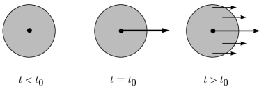
Figure 3: Elastic transition induced by an external heavy-quark current.

It is more conventional to write the above matrix element in terms of an elastic form factor $F_{\rm el}(q^{2})$ depending on the momentum transfer $q^{2}=(p-p^{\prime})^{2}$:

$$\langle\bar{B}(v^{\prime})|\,\bar{b}\,\gamma^{\mu}b\,|\bar{B}(v)\rangle=F_{\rm el}(q^{2})\,(p+p^{\prime})^{\mu}\,,$$ (18)

where $p^{(}\phantom{}{}^{\prime}\phantom{}{}^{)}=m_{B}v^{(}\phantom{}{}^{\prime}\phantom{}{}^{)}$. Comparing this with (16), we find that

$$F_{\rm el}(q^{2})=\xi(v\cdot v^{\prime})\,,\qquad q^{2}=-2m_{B}^{2}(v\cdot v^{\prime}-1)\,.$$ (19)

Because of current conservation, the elastic form factor is normalized to unity at $q^{2}=0$. This condition implies the normalization of the Isgur–Wise function at the kinematic point $v\cdot v^{\prime}=1$, i.e. for $v=v^{\prime}$:

$$\xi(1)=1\,.$$ (20)

It is in accordance with the intuitive argument that the probability for an elastic transition is unity if there is no velocity change. Since for $v=v^{\prime}$ the daughter meson is at rest in the rest frame of the parent meson, the point $v\cdot v^{\prime}=1$ is referred to as the zero-recoil limit.

We can now use the flavour symmetry to replace the $b$ quark in the final-state meson by a $c$ quark, thereby turning the $B$ meson into a $D$ meson. Then the scattering process turns into a weak decay process. In the infinite-mass limit, the replacement $b_{v^{\prime}}\to c_{v^{\prime}}$ is a symmetry transformation, under which the effective Lagrangian is invariant. Hence, the matrix element

$${1\over\sqrt{m_{B}m_{D}}}\,\langle D(v^{\prime})|\,\bar{c}_{v^{\prime}}\gamma^{\mu}b_{v}\,|\bar{B}(v)\rangle=\xi(v\cdot v^{\prime})\,(v+v^{\prime})^{\mu}$$ (21)

is still determined by the same function $\xi(v\cdot v^{\prime})$. This is interesting, since in general the matrix element of a flavour-changing current between two pseudoscalar mesons is described by two form factors:

$$\langle D(v^{\prime})|\,\bar{c}\,\gamma^{\mu}b\,|\bar{B}(v)\rangle=f_{+}(q^{2})\,(p+p^{\prime})^{\mu}-f_{-}(q^{2})\,(p-p^{\prime})^{\mu}\,.$$ (22)

Comparing the above two equations, we find that

$$f_{\pm}(q^{2}) = {m_{B}\pm m_{D}\over 2\sqrt{m_{B}m_{D}}}\,\xi(v\cdot v^{\prime})\,,$$

$$q^{2} = m_{B}^{2}+m_{D}^{2}-2m_{B}m_{D}\,v\cdot v^{\prime}\,.$$ (23)

Thus, the heavy-quark flavour symmetry relates two a priori independent form factors to one and the same function. Moreover, the normalization of the Isgur–Wise function at $v\cdot v^{\prime}=1$ now implies a non-trivial normalization of the form factors $f_{\pm}(q^{2})$ at the point of maximum momentum transfer, $q_{\rm max}^{2}=(m_{B}-m_{D})^{2}$:

$$f_{\pm}(q_{\rm max}^{2})={m_{B}\pm m_{D}\over 2\sqrt{m_{B}m_{D}}}\,.$$ (24)

The heavy-quark spin symmetry leads to additional relations among weak decay form factors. It can be used to relate matrix elements involving vector mesons to those involving pseudoscalar mesons. A vector meson with longitudinal polarization is related to a pseudoscalar meson by a rotation of the heavy-quark spin. Hence, the spin-symmetry transformation $c_{v^{\prime}}^{\Uparrow}\to c_{v^{\prime}}^{\Downarrow}$ relates $\bar{B}\to D$ with $\bar{B}\to D^{*}$ transitions. The result of this transformation is [27]:

$${1\over\sqrt{m_{B}m_{D^{*}}}}\,\langle D^{*}(v^{\prime},\varepsilon)|\,\bar{c}_{v^{\prime}}\gamma^{\mu}b_{v}\,|\bar{B}(v)\rangle = i\epsilon^{\mu\nu\alpha\beta}\,\varepsilon_{\nu}^{*}\,v^{\prime}_{\alpha}v_{\beta}\,\,\xi(v\cdot v^{\prime})\,,$$

$${1\over\sqrt{m_{B}m_{D^{*}}}}\,\langle D^{*}(v^{\prime},\varepsilon)|\,\bar{c}_{v^{\prime}}\gamma^{\mu}\gamma_{5}\,b_{v}\,|\bar{B}(v)\rangle = \Big{[}\varepsilon^{*\mu}\,(v\cdot v^{\prime}+1)-v^{\prime\mu}\,\varepsilon^{*}\!\cdot v\Big{]}\,\xi(v\cdot v^{\prime})\,,$$

where $\varepsilon$ denotes the polarization vector of the $D^{*}$ meson. Once again, the matrix elements are completely described in terms of the Isgur–Wise function. Now this is even more remarkable, since in general four form factors, $V(q^{2})$ for the vector current, and $A_{i}(q^{2})$, $i=0,1,2$, for the axial current, are required to parametrize these matrix elements. In the heavy-quark limit, they obey the relations [38]

$${m_{B}+m_{D^{*}}\over 2\sqrt{m_{B}m_{D^{*}}}}\,\xi(v\cdot v^{\prime}) = V(q^{2})=A_{0}(q^{2})=A_{1}(q^{2})$$

$$= \bigg{[}1-{q^{2}\over(m_{B}+m_{D})^{2}}\bigg{]}^{-1}\,A_{1}(q^{2})\,,$$

$$\phantom{\Bigg{[}}q^{2} = m_{B}^{2}+m_{D^{*}}^{2}-2m_{B}m_{D^{*}}\,v\cdot v^{\prime}\,.$$ (26)

Equations (2.3) and (2.3) summarize the relations imposed by heavy-quark symmetry on the weak decay form factors describing the semileptonic decay processes $\bar{B}\to D\,\ell\,\bar{\nu}$ and $\bar{B}\to D^{*}\ell\,\bar{\nu}$. These relations are model-independent consequences of QCD in the limit where $m_{b},m_{c}\gg\Lambda_{\rm QCD}$. They play a crucial role in the determination of the CKM matrix element $|V_{cb}|$. In terms of the recoil variable $w=v\cdot v^{\prime}$, the differential semileptonic decay rates in the heavy-quark limit become [39]:

$${{\rm d}\Gamma(\bar{B}\to D\,\ell\,\bar{\nu})\over{\rm d}w} = {G_{F}^{2}\over 48\pi^{3}}\,|V_{cb}|^{2}\,(m_{B}+m_{D})^{2}\,m_{D}^{3}\,(w^{2}-1)^{3/2}\,\xi^{2}(w)\,,$$

$$\phantom{\Bigg{[}}{{\rm d}\Gamma(\bar{B}\to D^{*}\ell\,\bar{\nu})\over{\rm d}w} = {G_{F}^{2}\over 48\pi^{3}}\,|V_{cb}|^{2}\,(m_{B}-m_{D^{*}})^{2}\,m_{D^{*}}^{3}\,\sqrt{w^{2}-1}\,(w+1)^{2}$$ (27)

$$\times\Bigg{[}1+{4w\over w+1}\,{m_{B}^{2}-2w\,m_{B}m_{D^{*}}+m_{D^{*}}^{2}\over(m_{B}-m_{D^{*}})^{2}}\Bigg{]}\,\xi^{2}(w)\,.$$

These expressions receive symmetry-breaking corrections, since the masses of the heavy quarks are not infinitely heavy. Perturbative corrections of order $\alpha_{s}^{n}(m_{Q})$ can be calculated order by order in perturbation theory. A more difficult task is to control the non-perturbative power corrections of order $(\Lambda_{\rm QCD}/m_{Q})^{n}$. The HQET provides a systematic framework for analysing these corrections. For the case of weak-decay form factors, the analysis of the $1/m_{Q}$ corrections was performed by Luke [40]. Later, Falk and the present author have also analysed the structure of $1/m_{Q}^{2}$ corrections for both meson and baryon weak decay form factors [32]. We shall not discuss these rather technical issues in detail, but only mention the most important result of Luke’s analysis. It concerns the zero-recoil limit, where an analogue of the Ademollo–Gatto theorem [41] can be proved. This is Luke’s theorem [40], which states that the matrix elements describing the leading $1/m_{Q}$ corrections to weak decay amplitudes vanish at zero recoil. This theorem is valid to all orders in perturbation theory [32, 42, 43]. Most importantly, it protects the $\bar{B}\to D^{*}\ell\,\bar{\nu}$ decay rate from receiving first-order $1/m_{Q}$ corrections at zero recoil [39]. (A similar statement is not true for the decay $\bar{B}\to D\,\ell\,\bar{\nu}$, however. The reason is simple but somewhat subtle. Luke’s theorem protects only those form factors not multiplied by kinematic factors that vanish for $v=v^{\prime}$. By angular momentum conservation, the two pseudoscalar mesons in the decay $\bar{B}\to D\,\ell\,\bar{\nu}$ must be in a relative $p$ wave, and hence the amplitude is proportional to the velocity $|\vec{v}_{D}|$ of the $D$ meson in the $B$-meson rest frame. This leads to a factor $(w^{2}-1)$ in the decay rate. In such a situation, form factors that are kinematically suppressed can contribute [38].)

2.4 Model-Independent Determination of $|V_{cb}|$

We will now discuss the most important application of the HQET in the context of semileptonic decays of $B$ mesons. A model-independent determination of the CKM matrix element $|V_{cb}|$ based on heavy-quark symmetry can be obtained by measuring the recoil spectrum of $D^{*}$ mesons produced in $\bar{B}\to D^{*}\ell\,\bar{\nu}$ decays [39]. In the heavy-quark limit, the differential decay rate for this process has been given in (2.3). In order to allow for corrections to that limit, we write

$${{\rm d}\Gamma(\bar{B}\to D^{*}\ell\,\bar{\nu})\over{\rm d}w} = {G_{F}^{2}\over 48\pi^{3}}\,(m_{B}-m_{D^{*}})^{2}\,m_{D^{*}}^{3}\sqrt{w^{2}-1}\,(w+1)^{2}$$

$$\mbox{}\times\Bigg{[}1+{4w\over w+1}\,{m_{B}^{2}-2w\,m_{B}m_{D^{*}}+m_{D^{*}}^{2}\over(m_{B}-m_{D^{*}})^{2}}\Bigg{]}\,|V_{cb}|^{2}\,{\cal{F}}^{2}(w)\,,$$

where the hadronic form factor ${\cal F}(w)$ coincides with the Isgur–Wise function up to symmetry-breaking corrections of order $\alpha_{s}(m_{Q})$ and $\Lambda_{\rm QCD}/m_{Q}$. The idea is to measure the product $|V_{cb}|\,{\cal F}(w)$ as a function of $w$, and to extract $|V_{cb}|$ from an extrapolation of the data to the zero-recoil point $w=1$, where the $B$ and the $D^{*}$ mesons have a common rest frame. At this kinematic point, heavy-quark symmetry helps to calculate the normalization ${\cal F}(1)$ with small and controlled theoretical errors. Since the range of $w$ values accessible in this decay is rather small ($1<w<1.5$), the extrapolation can be done using an expansion around $w=1$:

$${\cal F}(w)={\cal F}(1)\,\Big{[}1-\hat{\varrho}^{2}\,(w-1)+\dots\Big{]}\,.$$ (29)

The slope $\hat{\varrho}^{2}$ is treated as a fit parameter.

Figure 4: CLEO data for the product $|V_{cb}|\,{\cal F}(w)$, as extracted from the recoil spectrum in $\bar{B}\to D^{*}\ell\,\bar{\nu}$ decays [45]. The line shows a linear fit to the data.

Measurements of the recoil spectrum have been performed first by the ARGUS [44] and CLEO [45] Collaborations in experiments operating at the $\Upsilon(4s)$ resonance, and more recently by the ALEPH [46] and DELPHI [47] Collaborations at LEP. As an example, Fig. 4 shows the data reported by the CLEO Collaboration. The results obtained by the various experimental groups from a linear fit to their data are summarized in Table 1. The weighted average of these results is

$$|V_{cb}|\,{\cal F}(1) = (34.6\pm 1.7)\times 10^{-3}\,,$$

$$\hat{\varrho}^{2} = 0.82\pm 0.09\,.$$ (30)

The effect of a positive curvature of the form factor has been investigated by Stone [48], who finds that the value of $|V_{cb}|\,{\cal F}(1)$ may change by up to $+4\%$. We thus increase the above value by $(2\pm 2)\%$ and quote the final result as

$$|V_{cb}|\,{\cal F}(1)=(35.3\pm 1.8)\times 10^{-3}\,.$$ (31)

In future analyses, the extrapolation to zero recoil should be performed including higher-order terms in the expansion (29). It can be shown in a model-independent way that the shape of the form factor is highly constrained by analyticity and unitarity requirements [49, 50]. In particular, the curvature at $w=1$ is strongly correlated with the slope of the form factor. For the value of $\hat{\varrho}^{2}$ given in (2.4), one obtains a small positive curvature [50], in agreement with the assumption made in Ref. 48.

Table 1: Values for $|V_{cb}|\,{\cal F}(1)$ (in units of $10^{-3}$) and $\hat{\varrho}^{2}$ extracted from measurements of the recoil spectrum in $\bar{B}\to D^{*}\ell\,\bar{\nu}$ decays

	$|V_{cb}|\,{\cal F}(1)~{}(10^{-3})$	$\hat{\varrho}^{2}$
ARGUS	$38.8\pm 4.3\pm 2.5$	$1.17\pm 0.22\pm 0.06$
CLEO	$35.1\pm 1.9\pm 2.0$	$0.84\pm 0.12\pm 0.08$
ALEPH	$31.4\pm 2.3\pm 2.5$	$0.39\pm 0.21\pm 0.12$
DELPHI	$35.0\pm 1.9\pm 2.3$	$0.81\pm 0.16\pm 0.10$

Heavy-quark symmetry implies that the general structure of the symmetry-breaking corrections to the form factor at zero recoil is [39]

$${\cal F}(1)=\eta_{A}\,\bigg{(}1+0\times{\Lambda_{\rm QCD}\over m_{Q}}+\mbox{const}\times{\Lambda_{\rm QCD}^{2}\over m_{Q}^{2}}+\dots\bigg{)}\equiv\eta_{A}\,(1+\delta_{1/m^{2}})\,,$$ (32)

where $\eta_{A}$ is a short-distance correction arising from the (finite) renormalization of the flavour-changing axial current at zero recoil, and $\delta_{1/m^{2}}$ parametrizes second-order (and higher) power corrections. The absence of first-order power corrections at zero recoil is a consequence of Luke’s theorem [40]. The one-loop expression for $\eta_{A}$ has been known for a long time [23, 26, 51]:

$$\eta_{A}=1+{\alpha_{s}(M)\over\pi}\,\bigg{(}{m_{b}+m_{c}\over m_{b}-m_{c}}\,\ln{m_{b}\over m_{c}}-{8\over 3}\bigg{)}\simeq 0.96\,.$$ (33)

The scale $M$ in the running coupling constant can be fixed by adopting the prescription of Brodsky, Lepage and Mackenzie (BLM) [52], according to which it is identified with the average virtuality of the gluon in the one-loop diagrams that contribute to $\eta_{A}$. If $\alpha_{s}(M)$ is defined in the modified minimal subtraction ($\overline{\mbox{\sc ms}}$) scheme, the result is [53] $M\simeq 0.51\sqrt{m_{c}m_{b}}$. Several estimates of higher-order corrections to $\eta_{A}$ have been discussed. The next-to-leading order resummation of logarithms of the type $[\alpha_{s}\ln(m_{b}/m_{c})]^{n}$ leads to [54, 55] $\eta_{A}\simeq 0.985$. On the other hand, the resummation of “renormalon-chain” contributions of the form $\beta_{0}^{n-1}\alpha_{s}^{n}$, where $\beta_{0}$ is the first coefficient of the QCD $\beta$-function, gives [56, 57] $\eta_{A}\simeq 0.945$. Using these partial resummations to estimate the uncertainty results in $\eta_{A}=0.965\pm 0.020$. Recently, Czarnecki has improved this estimate by calculating $\eta_{A}$ at two-loop order [58]. His result,

$$\eta_{A}=0.960\pm 0.007\,,$$ (34)

is in excellent agreement with the BLM-improved one-loop estimate (33). Here the error is taken to be the size of the two-loop correction.

The analysis of the power corrections $\delta_{1/m^{2}}$ is more difficult, since it cannot rely on perturbation theory. Three approaches have been discussed: in the “exclusive approach”, all $1/m_{Q}^{2}$ operators in the HQET are classified and their matrix elements estimated, leading to [32, 59] $\delta_{1/m^{2}}=-(3\pm 2)\%$; the “inclusive approach” has been used to derive the bound $\delta_{1/m^{2}}<-3\%$, and to estimate that [60]^, $\delta_{1/m^{2}}=-(7\pm 3)\%$; the “hybrid approach” combines the virtues of the former two to obtain a more restrictive lower bound on $\delta_{1/m^{2}}$. This leads to [62]

$$\delta_{1/m^{2}}=-0.055\pm 0.025\,.$$ (35)

Combining the above results, adding the theoretical errors linearly to be conservative, gives

$${\cal F}(1)=0.91\pm 0.03$$ (36)

for the normalization of the hadronic form factor at zero recoil. Thus, the corrections to the heavy-quark limit amount to a moderate decrease of the form factor of about 10%. This can be used to extract from the experimental result (31) the model-independent value

$$|V_{cb}|=(38.8\pm 2.0_{\rm exp}\pm 1.2_{\rm th})\times 10^{-3}\,.$$ (37)

3 Heavy-Quark Effective Theory

3.1 The Effective Lagrangian

The effects of a very heavy particle often become irrelevant at low energies. It is then useful to construct a low-energy effective theory, in which this heavy particle no longer appears [63]. Eventually, this effective theory will be easier to deal with than the full theory. A familiar example is Fermi’s theory of the weak interactions. For the description of weak decays of hadrons, the weak interactions can be approximated by point-like four-fermion couplings, governed by a dimensionful coupling constant $G_{F}$. Only at energies much larger than the masses of hadrons can the effects of the intermediate vector bosons, $W$ and $Z$, be resolved.

The process of removing the degrees of freedom of a heavy particle involves the following steps [64]^-[66]: one first identifies the heavy-particle fields and “integrates them out” in the generating functional of the Green functions of the theory. This is possible since at low energies the heavy particle does not appear as an external state. However, although the action of the full theory is usually a local one, what results after this first step is a non-local effective action. The non-locality is related to the fact that in the full theory the heavy particle with mass $M$ can appear in virtual processes and propagate over a short but finite distance $\Delta x\sim 1/M$. Thus, a second step is required to obtain a local effective Lagrangian: the non-local effective action is rewritten as an infinite series of local terms using the OPE [16, 17]. Roughly speaking, this corresponds to an expansion in powers of $1/M$. It is in this step that the short- and long-distance physics is disentangled. The long-distance physics corresponds to interactions at low energies and is the same in the full and the effective theory. But short-distance effects arising from quantum corrections involving large virtual momenta (of order $M$) are not reproduced in the effective theory, once the heavy particle has been integrated out. In a third step, they have to be added in a perturbative way using renormalization-group techniques. These short-distance effects lead to a renormalization of the coefficients of the local operators in the effective Lagrangian. An example is the effective Lagrangian for non-leptonic weak decays, in which radiative corrections from hard gluons with virtual momenta in the range between $M_{W}$ and some renormalization scale $\mu\sim 1$ GeV give rise to Wilson coefficients, which renormalize the local four-fermion interactions [67]^-[69].

Figure 5: Philosophy of the heavy-quark effective theory.

The heavy-quark effective theory (HQET) is constructed to provide a simplified description of processes where a heavy quark interacts with light degrees of freedom predominantly by the exchange of soft gluons [70]^-[80]. Clearly, $m_{Q}$ is the high-energy scale in this case, and $\Lambda_{\rm QCD}$ is the scale of the hadronic physics we are interested in. The situation is illustrated in Fig. 5. At short distances, i.e. for energy scales larger than the heavy-quark mass, the physics is perturbative and described by ordinary QCD. For mass scales much below the heavy-quark mass, the physics is complicated and non-perturbative because of confinement. Our goal is to obtain a simplified description in this region using an effective field theory. To separate short- and long-distance effects, we introduce a separation scale $\mu$ such that $\Lambda_{\rm QCD}\ll\mu\ll m_{Q}$. The HQET will be constructed in such a way that it is identical to QCD in the long-distance region, i.e. for scales below $\mu$. In the short-distance region, the effective theory is incomplete, however, since some high-momentum modes have been integrated out from the full theory. The fact that the physics must be independent of the arbitrary scale $\mu$ allows us to derive renormalization-group equations, which can be employed to deal with the short-distance effects in an efficient way.

Compared with most effective theories, in which the degrees of freedom of a heavy particle are removed completely from the low-energy theory, the HQET is special in that its purpose is to describe the properties and decays of hadrons which do contain a heavy quark. Hence, it is not possible to remove the heavy quark completely from the effective theory. What is possible is to integrate out the “small components” in the full heavy-quark spinor, which describe the fluctuations around the mass shell.

The starting point in the construction of the low-energy effective theory is the observation that a very heavy quark bound inside a hadron moves more or less with the hadron’s velocity $v$, and is almost on shell. Its momentum can be written as

$$p_{Q}^{\mu}=m_{Q}v^{\mu}+k^{\mu}\,,$$ (38)

where the components of the so-called residual momentum $k$ are much smaller than $m_{Q}$. Note that $v$ is a four-velocity, so that $v^{2}=1$. Interactions of the heavy quark with light degrees of freedom change the residual momentum by an amount of order $\Delta k\sim\Lambda_{\rm QCD}$, but the corresponding changes in the heavy-quark velocity vanish as $\Lambda_{\rm QCD}/m_{Q}\to 0$. In this situation, it is appropriate to introduce large- and small-component fields, $h_{v}$ and $H_{v}$, by

$$h_{v}(x)=e^{im_{Q}v\cdot x}\,P_{+}\,Q(x)\,,\qquad H_{v}(x)=e^{im_{Q}v\cdot x}\,P_{-}\,Q(x)\,,$$ (39)

where $P_{+}$ and $P_{-}$ are projection operators defined as

$$P_{\pm}={1\pm\hbox to0.0pt{/\hss}v\over 2}\,.$$ (40)

It follows that

$$Q(x)=e^{-im_{Q}v\cdot x}\,[h_{v}(x)+H_{v}(x)]\,.$$ (41)

Because of the projection operators, the new fields satisfy $\hbox to0.0pt{/\hss}v\,h_{v}=h_{v}$ and $\hbox to0.0pt{/\hss}v\,H_{v}=-H_{v}$. In the rest frame, i.e. for $v^{\mu}=(1,0,0,0)$, $h_{v}$ corresponds to the upper two components of $Q$, while $H_{v}$ corresponds to the lower ones. Whereas $h_{v}$ annihilates a heavy quark with velocity $v$, $H_{v}$ creates a heavy antiquark with velocity $v$.

In terms of the new fields, the QCD Lagrangian for a heavy quark takes the form

$${\cal L}_{Q} = \bar{Q}\,(i\,\hbox to0.0pt{\,/\hss}D-m_{Q})\,Q$$ (42)

$$= \bar{h}_{v}\,iv\!\cdot\!D\,h_{v}-\bar{H}_{v}\,(iv\!\cdot\!D+2m_{Q})\,H_{v}$$

$$\mbox{}+\bar{h}_{v}\,i\,\hbox to0.0pt{\,/\hss}D_{\perp}H_{v}+\bar{H}_{v}\,i\,\hbox to0.0pt{\,/\hss}D_{\perp}h_{v}\,,$$

where $D_{\perp}^{\mu}=D^{\mu}-v^{\mu}\,v\cdot D$ is orthogonal to the heavy-quark velocity: $v\cdot D_{\perp}=0$. In the rest frame, $D_{\perp}^{\mu}=(0,\vec{D}\,)$ contains the spatial components of the covariant derivative. From (42), it is apparent that $h_{v}$ describes massless degrees of freedom, whereas $H_{v}$ corresponds to fluctuations with twice the heavy-quark mass. These are the heavy degrees of freedom that will be eliminated in the construction of the effective theory. The fields are mixed by the presence of the third and fourth terms, which describe pair creation or annihilation of heavy quarks and antiquarks. As shown in the first diagram in Fig. 6, in a virtual process a heavy quark propagating forward in time can turn into an antiquark propagating backward in time, and then turn back into a quark. The energy of the intermediate quantum state $hh\bar{H}$ is larger than the energy of the initial heavy quark by at least $2m_{Q}$. Because of this large energy gap, the virtual quantum fluctuation can only propagate over a short distance $\Delta x\sim 1/m_{Q}$. On hadronic scales set by $R_{\rm had}\sim 1/\Lambda_{\rm QCD}$, the process essentially looks like a local interaction of the form

$$\bar{h}_{v}\,i\,\hbox to0.0pt{\,/\hss}D_{\perp}\,{1\over 2m_{Q}}\,i\,\hbox to0.0pt{\,/\hss}D_{\perp}h_{v}\,,$$ (43)

where we have simply replaced the propagator for $H_{v}$ by $1/2m_{Q}$. A more correct treatment is to integrate out the small-component field $H_{v}$, thereby deriving a non-local effective action for the large-component field $h_{v}$, which can then be expanded in terms of local operators. Before doing this, let us mention a second type of virtual corrections involving pair creation, namely heavy-quark loops. An example is shown in the second diagram in Fig. 6. Heavy-quark loops cannot be described in terms of the effective fields $h_{v}$ and $H_{v}$, since the quark velocities inside a loop are not conserved and are in no way related to hadron velocities. However, such short-distance processes are proportional to the small coupling constant $\alpha_{s}(m_{Q})$ and can be calculated in perturbation theory. They lead to corrections that are added onto the low-energy effective theory in the renormalization procedure.

Figure 6: Virtual fluctuations involving pair creation of heavy quarks. In the first diagram, time flows to the right.

On a classical level, the heavy degrees of freedom represented by $H_{v}$ can be eliminated using the equation of motion. Taking the variation of the Lagrangian with respect to the field $\bar{H}_{v}$, we obtain

$$(iv\!\cdot\!D+2m_{Q})\,H_{v}=i\,\hbox to0.0pt{\,/\hss}D_{\perp}h_{v}\,.$$ (44)

This equation can formally be solved to give

$$H_{v}={1\over 2m_{Q}+iv\!\cdot\!D}\,i\,\hbox to0.0pt{\,/\hss}D_{\perp}h_{v}\,,$$ (45)

showing that the small-component field $H_{v}$ is indeed of order $1/m_{Q}$. We can now insert this solution into (42) to obtain the “non-local effective Lagrangian”

$${\cal L}_{\rm eff}=\bar{h}_{v}\,iv\!\cdot\!D\,h_{v}+\bar{h}_{v}\,i\,\hbox to0.0pt{\,/\hss}D_{\perp}\,{1\over 2m_{Q}+iv\!\cdot\!D}\,i\,\hbox to0.0pt{\,/\hss}D_{\perp}h_{v}\,.$$ (46)

Clearly, the second term corresponds to the first class of virtual processes shown in Fig. 6.

It is possible to derive this Lagrangian in a more elegant way by manipulating the generating functional for QCD Green’s functions containing heavy-quark fields [80]. To this end, one starts from the field redefinition (41) and couples the large-component fields $h_{v}$ to external sources $\rho_{v}$. Green’s functions with an arbitrary number of $h_{v}$ fields can be constructed by taking derivatives with respect to $\rho_{v}$. No sources are needed for the heavy degrees of freedom represented by $H_{v}$. The functional integral over these fields is Gaussian and can be performed explicitly, leading to the effective action

$$S_{\rm eff}=\int\!{\rm d}^{4}x\,{\cal L}_{\rm eff}-i\ln\Delta\,,$$ (47)

with ${\cal L}_{\rm eff}$ as given in (46). The appearance of the logarithm of the determinant

$$\Delta=\exp\bigg{(}{1\over 2}\,{\rm Tr}\,\ln\big{[}2m_{Q}+iv\!\cdot\!D-i\eta\big{]}\bigg{)}$$ (48)

is a quantum effect not present in the classical derivation presented above. However, in this case the determinant can be regulated in a gauge-invariant way, and by choosing the gauge $v\cdot A=0$ one can show that $\ln\Delta$ is just an irrelevant constant [80, 81].

Because of the phase factor in (41), the $x$ dependence of the effective heavy-quark field $h_{v}$ is weak. In momentum space, derivatives acting on $h_{v}$ correspond to powers of the residual momentum $k$, which by construction is much smaller than $m_{Q}$. Hence, the non-local effective Lagrangian (46) allows for a derivative expansion in powers of $iD/m_{Q}$:

$${\cal L}_{\rm eff}=\bar{h}_{v}\,iv\!\cdot\!D\,h_{v}+{1\over 2m_{Q}}\,\sum_{n=0}^{\infty}\,\bar{h}_{v}\,i\,\hbox to0.0pt{\,/\hss}D_{\perp}\,\bigg{(}-{iv\cdot D\over 2m_{Q}}\bigg{)}^{n}\,i\,\hbox to0.0pt{\,/\hss}D_{\perp}h_{v}\,.$$ (49)

Taking into account that $h_{v}$ contains a $P_{+}$ projection operator, and using the identity

$$P_{+}\,i\,\hbox to0.0pt{\,/\hss}D_{\perp}\,i\,\hbox to0.0pt{\,/\hss}D_{\perp}P_{+}=P_{+}\,\bigg{[}(iD_{\perp})^{2}+{g_{s}\over 2}\,\sigma_{\mu\nu}\,G^{\mu\nu}\bigg{]}\,P_{+}\,,$$ (50)

where $[iD^{\mu},iD^{\nu}]=ig_{s}G^{\mu\nu}$ is the gluon field-strength tensor, one finds that [78, 79]

$${\cal L}_{\rm eff}=\bar{h}_{v}\,iv\!\cdot\!D\,h_{v}+{1\over 2m_{Q}}\,\bar{h}_{v}\,(iD_{\perp})^{2}\,h_{v}+{g_{s}\over 4m_{Q}}\,\bar{h}_{v}\,\sigma_{\mu\nu}\,G^{\mu\nu}\,h_{v}+O(1/m_{Q}^{2})\,.$$ (51)

In the limit $m_{Q}\to\infty$, only the first terms remains:

$${\cal L}_{\infty}=\bar{h}_{v}\,iv\!\cdot\!D\,h_{v}\,.$$ (52)

This is the effective Lagrangian of the HQET. It gives rise to the Feynman rules depicted in Fig. 7.

Figure 7: Feynman rules of the HQET ($i,j$ and $a$ are colour indices). A heavy quark is represented by a double line labelled by the velocity $v$ and the residual momentum $k$. The velocity $v$ is conserved by the strong interactions.

Let us take a moment to study the symmetries of this Lagrangian [28]. Since there appear no Dirac matrices, interactions of the heavy quark with gluons leave its spin unchanged. Associated with this is an SU(2) symmetry group, under which ${\cal L}_{\infty}$ is invariant. The action of this symmetry on the heavy-quark fields becomes most transparent in the rest frame, where the generators $S^{i}$ of SU(2) can be chosen as

$$S^{i}={1\over 2}\left(\begin{array}[]{cc}\sigma^{i}{}&~{}0\\ 0{}&~{}\sigma^{i}\end{array}\right)\,,\qquad[S^{i},S^{j}]=i\epsilon^{ijk}S^{k}\,.$$ (53)

Here $\sigma^{i}$ are the Pauli matrices. An infinitesimal SU(2) transformation $h_{v}\to(1+i\vec{\epsilon}\cdot\vec{S}\,)\,h_{v}$ leaves the Lagrangian invariant:

$$\delta{\cal L}_{\infty}=\bar{h}_{v}\,[iv\!\cdot\!D,i\vec{\epsilon}\cdot\vec{S}\,]\,h_{v}=0\,.$$ (54)

Another symmetry of the HQET arises since the mass of the heavy quark does not appear in the effective Lagrangian. For $N_{h}$ heavy quarks moving at the same velocity, eq. (52) can be extended by writing

$${\cal L}_{\infty}=\sum_{i=1}^{N_{h}}\,\bar{h}_{v}^{i}\,iv\!\cdot\!D\,h_{v}^{i}\,.$$ (55)

This is invariant under rotations in flavour space. When combined with the spin symmetry, the symmetry group is promoted to SU$(2N_{h})$. This is the heavy-quark spin–flavour symmetry [27, 28]. Its physical content is that, in the limit $m_{Q}\to\infty$, the strong interactions of a heavy quark become independent of its mass and spin.

Consider now the operators appearing at order $1/m_{Q}$ in the effective Lagrangian (51). They are easiest to identify in the rest frame. The first operator,

$${\cal O}_{\rm kin}={1\over 2m_{Q}}\,\bar{h}_{v}\,(iD_{\perp})^{2}\,h_{v}\to-{1\over 2m_{Q}}\,\bar{h}_{v}\,(i\vec{D}\,)^{2}\,h_{v}\,,$$ (56)

is the gauge-covariant extension of the kinetic energy arising from the off-shell residual motion of the heavy quark. The second operator is the non-abelian analogue of the Pauli interaction, which describes the chromo-magnetic coupling of the heavy-quark spin to the gluon field:

$${\cal O}_{\rm mag}={g_{s}\over 4m_{Q}}\,\bar{h}_{v}\,\sigma_{\mu\nu}\,G^{\mu\nu}\,h_{v}\to-{g_{s}\over m_{Q}}\,\bar{h}_{v}\,\vec{S}\!\cdot\!\vec{B}_{c}\,h_{v}\,.$$ (57)

Here $\vec{S}$ is the spin operator defined in (53), and $B_{c}^{i}=-\frac{1}{2}\epsilon^{ijk}G^{jk}$ are the components of the chromo-magnetic field. The chromo-magnetic interaction is a relativistic effect, which scales like $1/m_{Q}$. This is the origin of the heavy-quark spin symmetry.

3.2 The Residual Mass Term and the Definition of the Heavy-Quark Mass

The choice of the expansion parameter in the HQET, i.e. the definition of the heavy-quark mass $m_{Q}$, deserves some comments. In the derivation presented earlier in this section, we chose $m_{Q}$ to be the “mass in the Lagrangian”, and using this parameter in the phase redefinition in (41) we obtained the effective Lagrangian (52), in which the heavy-quark mass no longer appears. However, this treatment has its subtleties. The symmetries of the HQET allow a “residual mass” $\delta m$ for the heavy quark, provided that $\delta m$ is of order $\Lambda_{\rm QCD}$ and is the same for all heavy-quark flavours. Even if we arrange that such a mass term is not present at the tree level, it will in general be induced by quantum corrections. (This is unavoidable if the theory is regulated with a dimensionful cutoff.) Therefore, instead of (52) we should write the effective Lagrangian in the more general form [31]:

$$h_{v}(x) = e^{im_{Q}v\cdot x}\,P_{+}\,Q(x)$$

$$\Rightarrow\qquad{\cal L}_{\infty} = \bar{h}_{v}\,iv\!\cdot\!D\,h_{v}-\delta m\,\bar{h}_{v}h_{v}\,.$$ (58)

If we redefine the expansion parameter according to $m_{Q}\to m_{Q}+\Delta m$, the residual mass changes in the opposite way: $\delta m\to\delta m-\Delta m$. This implies that there is a unique choice of the expansion parameter $m_{Q}$ such that $\delta m=0$. Requiring $\delta m=0$, as it is usually done implicitly in the HQET, defines a heavy-quark mass, which in perturbation theory coincides with the pole mass [82]. This, in turn, defines for each heavy hadron a parameter $\bar{\Lambda}$ (sometimes called the “binding energy”) through

$$\bar{\Lambda}=(m_{H}-m_{Q})\Big{|}_{m_{Q}\to\infty}\,.$$ (59)

If one prefers to work with another choice of the expansion parameter, the values of non-perturbative parameters such as $\bar{\Lambda}$ change, but at the same time one has to include the residual mass term in the HQET Lagrangian. It can be shown that the various parameters that depend on the definition of $m_{Q}$ enter the predictions for all physical observables in such a way that the results are independent of which particular choice one adopts [31].

There is one more subtlety hidden in the above discussion. The quantities $m_{Q}$, $\bar{\Lambda}$ and $\delta m$ are non-perturbative parameters of the HQET, which have a similar status as the vacuum condensates in QCD phenomenology [83]. These parameters cannot be defined unambiguously in perturbation theory. The reason lies in the divergent behaviour of perturbative expansions in large orders, which is associated with the existence of singularities along the real axis in the Borel plane, the so-called renormalons [84]^-[92]. For instance, the perturbation series which relates the pole mass $m_{Q}$ of a heavy quark to its bare mass,

$$m_{Q}=m_{Q}^{\rm bare}\,\Big{\{}1+c_{1}\,\alpha_{s}(m_{Q})+c_{2}\,\alpha_{s}^{2}(m_{Q})+\dots+c_{n}\,\alpha_{s}^{n}(m_{Q})+\dots\Big{\}}\,,$$ (60)

contains numerical coefficients $c_{n}$ that grow as $n!$ for large $n$, rendering the series divergent and not Borel summable [93, 94]. The best one can achieve is to truncate the perturbation series at the minimal term, but this leads to an unavoidable arbitrariness of order $\Delta m_{Q}\sim\Lambda_{\rm QCD}$ (the size of the minimal term). This observation, which at first sight seems a serious problem for QCD phenomenology, should actually not come as a surprise. We know that because of confinement quarks do not appear as physical states in nature. Hence, there is no unique way to define their on-shell properties such as a pole mass. In view of this, it is actually remarkable that QCD perturbation theory “knows” about its incompleteness and indicates, through the appearance of renormalon singularities, the presence of non-perturbative effects. We must first specify a scheme how to truncate the QCD perturbation series before non-perturbative statements such as $\delta m=0$ become meaningful, and hence before non-perturbative parameters such as $m_{Q}$ and $\bar{\Lambda}$ become well-defined quantities. The actual values of these parameters will depend on this scheme.

We stress that the “renormalon ambiguities” are not a conceptual problem for the heavy-quark expansion. In fact, it can be shown quite generally that these ambiguities cancel in all predictions for physical observables [95]^-[97]. The way the cancellations occur is intricate, however. The generic structure of the heavy-quark expansion for an observable is of the form:

$$\mbox{observable}\sim C[\alpha_{s}(m_{Q})]\,\bigg{(}1+{\Lambda\over m_{Q}}+\dots\bigg{)}\,.$$ (61)

Here $C[\alpha_{s}(m_{Q})]$ represents a perturbative coefficient function, and $\Lambda$ is a dimensionful non-perturbative parameter. The truncation of the perturbation series defining the coefficient function leads to an arbitrariness of order $\Lambda_{\rm QCD}/m_{Q}$, which precisely cancels against a corresponding arbitrariness of order $\Lambda_{\rm QCD}$ in the definition of the non-perturbative parameter $\Lambda$.

The renormalon problem poses itself when one imagines to apply perturbation theory in very high orders. In practise, the perturbative coefficients are known to finite order in $\alpha_{s}$ (at best to two-loop accuracy), and to be consistent one should use them in connection with the pole mass (and $\bar{\Lambda}$ etc.) defined to the same order. For completeness, we note that for the “one-loop pole masses” of the heavy quarks we shall adopt the values

$$m_{b}=4.8~{}\mbox{GeV}\,,\qquad m_{c}=1.4~{}\mbox{GeV}\,.$$ (62)

Their difference satisfies the constraint in (15).

4 Inclusive Decay Rates

Inclusive decay rates determine the probability of the decay of a particle into the sum of all possible final states with a given set of quantum numbers. An example is provided by the inclusive semileptonic decay rate of the $B$ meson, $\Gamma(\bar{B}\to X_{c}\,\ell\,\bar{\nu})$, where the final state consists of a lepton–neutrino pair accompanied by any number of hadrons with total charm-quark number $n_{c}=1$. Here we shall discuss the theoretical description of inclusive decays of hadrons containing a heavy quark [98]^-[106]. From the theoretical point of view, such decays have two advantages: first, bound-state effects related to the initial state (such as the “Fermi motion” of the heavy quark inside the hadron) can be accounted for in a systematic way using the heavy-quark expansion, in much the same way as explained in the previous sections; secondly, the fact that the final state consists of a sum over many hadronic channels eliminates bound-state effects related to the properties of individual hadrons. This second feature is based on a hypothesis known as quark–hadron duality, which is an important concept in QCD phenomenology. The assumption of duality is that cross sections and decay rates, which are defined in the physical region (i.e. the region of time-like momenta), are calculable in QCD after a “smearing” or “averaging” procedure has been applied [107]. In semileptonic decays, it is the integration over the lepton and neutrino phase space that provides a “smearing” over the invariant hadronic mass of the final state (so-called “global” duality). For non-leptonic decays, on the other hand, the total hadronic mass is fixed, and it is only the fact that one sums over many hadronic states that provides an “averaging” (so-called “local” duality). Clearly, local duality is a stronger assumption than global duality. It is important to stress that quark–hadron duality cannot yet be derived from first principles, although it is a necessary assumption for many applications of QCD. The validity of global duality has been tested experimentally using data on hadronic $\tau$ decays [21]. A more formal attempt to address the problem of quark–hadron duality can be found in Ref. 108.

Using the optical theorem, the inclusive decay width of a hadron $H_{b}$ containing a $b$ quark can be written in the form

$$\Gamma(H_{b}\to X)={1\over 2m_{H_{b}}}\,2\,\mbox{Im}\,\langle H_{b}|\,{\bf T}\,|H_{b}\rangle\,,$$ (63)

where the transition operator ${\bf T}$ is given by

$${\bf T}=i\!\int{\rm d}^{4}x\,T\{\,{\cal L}_{\rm eff}(x),{\cal L}_{\rm eff}(0)\,\}\,.$$ (64)

In fact, inserting a complete set of states inside the time-ordered product, we recover the standard expression

$$\Gamma(H_{b}\to X)={1\over 2m_{H_{b}}}\,\sum_{X}\,(2\pi)^{4}\,\delta^{4}(p_{H}-p_{X})\,|\langle X|\,{\cal L}_{\rm eff}\,|H_{b}\rangle|^{2}$$ (65)

for the decay rate. Here ${\cal L}_{\rm eff}$ is the effective weak Lagrangian corrected for short-distance effects [67, 68, 109]^-[111] arising from the exchange of gluons with virtualities between $m_{W}$ and $m_{b}$. If some quantum numbers of the final states $X$ are specified, the sum over intermediate states is to be restricted appropriately. In the case of the inclusive semileptonic decay rate, for instance, the sum would include only those states $X$ containing a lepton–neutrino pair.

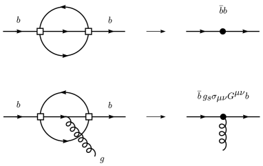
Figure 8: Perturbative contributions to the transition operator ${\bf T}$ (left), and the corresponding operators in the OPE (right). The open squares represent a four-fermion interaction of the effective Lagrangian ${\cal L}_{\rm eff}$, while the black circles represent local operators in the OPE.

In perturbation theory, some contributions to the transition operator are given by the two-loop diagrams shown on the left-hand side in Fig. 8. Because of the large mass of the $b$ quark, the momenta flowing through the internal lines in these diagrams are large. It is thus possible to construct an OPE for the transition operator, in which ${\bf T}$ is represented as a series of local operators containing the heavy-quark fields. The operator with the lowest dimension, $d=3$, is $\bar{b}b$. It arises from integrating over the internal lines in the first diagram shown in the figure. The only gauge-invariant operator with dimension $d=4$ is $\bar{b}\,i\hbox to0.0pt{\,/\hss}D\,b$; however, the equation of motion implies that between physical states this operator can be replaced by $m_{b}\bar{b}b$. The first operator that is different from $\bar{b}b$ has dimension $d=5$ and contains the gluon field. It is given by $\bar{b}\,g_{s}\sigma_{\mu\nu}G^{\mu\nu}b$. This operator arises from diagrams in which a gluon is emitted from one of the internal lines, such as the second diagram shown in the figure.

For dimensional reasons, the matrix elements of such higher-dimensional operators are suppressed by inverse powers of the heavy-quark mass. Thus, any inclusive decay rate of a hadron $H_{b}$ can be written in the form [99]^-[101]:

$$\Gamma(H_{b}\to X_{f})={G_{F}^{2}m_{b}^{5}\over 192\pi^{3}}\,\bigg{\{}c_{3}^{f}\,\langle\bar{b}b\rangle_{H}+c_{5}^{f}\,{\langle\bar{b}\,g_{s}\sigma_{\mu\nu}G^{\mu\nu}b\rangle_{H}\over m_{b}^{2}}+\dots\bigg{\}}\,,$$ (66)

where the prefactor arises naturally from the loop integrations, $c_{n}^{f}$ are calculable coefficient functions (which also contain the relevant CKM matrix elements) depending on the quantum numbers $f$ of the final state, and $\langle O\rangle_{H}$ are the (normalized) forward matrix elements of local operators, for which we use the short-hand notation

$$\langle O\rangle_{H}={1\over 2m_{H_{b}}}\,\langle H_{b}|\,O\,|H_{b}\rangle\,.$$ (67)

In the next step, these matrix elements are systematically expanded in powers of $1/m_{b}$, using the technology of the HQET. Introducing the velocity-dependent fields $b_{v}$ of the HQET, where $v$ denotes the velocity of the hadron $H_{b}$, one finds [32, 101, 102]

$$\langle\bar{b}b\rangle_{H} = 1-{\mu_{\pi}^{2}(H_{b})-\mu_{G}^{2}(H_{b})\over 2m_{b}^{2}}+O(1/m_{b}^{3})\,,$$

$$\langle\bar{b}\,g_{s}\sigma_{\mu\nu}G^{\mu\nu}b\rangle_{H} = 2\mu_{G}^{2}(H_{b})+O(1/m_{b})\,,$$ (68)

where we have defined the HQET matrix elements

$$\mu_{\pi}^{2}(H_{b}) = {1\over 2m_{H_{b}}}\,\langle H_{b}(v)|\,\bar{b}_{v}\,(i\vec{D})^{2}\,b_{v}\,|H_{b}(v)\rangle\,,$$

$$\mu_{G}^{2}(H_{b}) = {1\over 2m_{H_{b}}}\,\langle H_{b}(v)|\,\bar{b}_{v}{g_{s}\over 2}\sigma_{\mu\nu}G^{\mu\nu}b_{v}\,|H_{b}(v)\rangle\,.$$ (69)

Here $(i\vec{D})^{2}=(iv\cdot D)^{2}-(iD)^{2}$; in the rest frame, this is the square of the operator for the spatial momentum of the heavy quark. Inserting these results into (66), we obtain

$$\Gamma(H_{b}\to X_{f})={G_{F}^{2}m_{b}^{5}\over 192\pi^{3}}\,\bigg{\{}c_{3}^{f}\,\bigg{(}1-{\mu_{\pi}^{2}(H_{b})\over 2m_{b}^{2}}\bigg{)}+(4c_{5}^{f}+c_{3}^{f})\,{\mu_{G}^{2}(H_{b})\over 2m_{b}^{2}}+\dots\bigg{\}}\,.$$ (70)

It is instructive to understand the appearance of the “kinetic energy” contribution $\mu_{\pi}^{2}$, which is the gauge-covariant extension of the square of the $b$-quark momentum inside the heavy hadron. This contribution is the field-theory analogue of the Lorentz factor $(1-\vec{v}_{b}^{\,2})^{1/2}\simeq 1-\vec{p}_{b}^{\,2}/2m_{b}^{2}$, in accordance with the fact that the lifetime, $\tau=1/\Gamma$, for a moving particle increases due to time dilation.

The main result of the heavy-quark expansion for inclusive decay rates is that the free quark decay (i.e. the parton model) provides the first term in a systematic $1/m_{b}$ expansion, i.e.

$$\Gamma(H_{b}\to X_{f})={G_{F}^{2}m_{b}^{5}\over 192\pi^{3}}\,c_{3}^{f}\,\Big{\{}1+O(1/m_{b}^{2})\Big{\}}\,.$$ (71)

For dimensional reasons, the free-quark decay rate is proportional to the fifth power of the $b$-quark mass. The non-perturbative corrections to this picture, which arise from bound-state effects inside the hadron $H_{b}$, are suppressed by (at least) two powers of the heavy-quark mass, i.e. they are of relative order $(\Lambda_{\rm QCD}/m_{b})^{2}$. Note that the absence of first-order power corrections is a simple consequence of the equation of motion, as there is no independent gauge-invariant operator of dimension $d=4$ that could appear in the OPE. The fact that bound-state effects in inclusive decays are strongly suppressed explains a posteriori the success of the parton model in describing such processes.

The hadronic matrix elements appearing in the heavy-quark expansion (70) can be determined to some extent from the known masses of heavy hadron states. For the $B$ meson, one finds that [32]

$$\mu_{\pi}^{2}(B) = -\lambda_{1}=(0.3\pm 0.2)~{}\mbox{GeV}^{2}\,,$$

$$\mu_{G}^{2}(B) = 3\lambda_{2}={3\over 4}\,(m_{B^{*}}^{2}-m_{B}^{2})\simeq 0.36~{}\mbox{GeV}^{2}\,,$$ (72)

where $\lambda_{1}$ and $\lambda_{2}$ are the parameters appearing in the mass formula (3), and their numerical values have been taken from (14) and (8). For the ground-state baryon $\Lambda_{b}$, in which the light constituents have total spin zero, it follows that

$$\mu_{G}^{2}(\Lambda_{b})=0\,,$$ (73)

while the matrix element $\mu_{\pi}^{2}(\Lambda_{b})$ obeys the relation

$$(m_{\Lambda_{b}}-m_{\Lambda_{c}})-(\overline{m}_{B}-\overline{m}_{D})=\Big{[}\mu_{\pi}^{2}(B)-\mu_{\pi}^{2}(\Lambda_{b})\Big{]}\,\bigg{(}{1\over 2m_{c}}-{1\over 2m_{b}}\bigg{)}+O(1/m_{Q}^{2})\,,$$ (74)

where $\overline{m}_{B}$ and $\overline{m}_{D}$ denote the spin-averaged masses introduced in connection with (13). With the value of $m_{\Lambda_{b}}$ given in (11), this leads to

$$\mu_{\pi}^{2}(B)-\mu_{\pi}^{2}(\Lambda_{b})=(0.01\pm 0.03)~{}\mbox{GeV}^{2}\,.$$ (75)

What remains to be calculated, then, is the coefficient functions $c_{n}^{f}$ for a given inclusive decay channel. We shall now discuss two important applications of this general formalism.

4.1 Determination of $|V_{cb}|$ from Inclusive Semileptonic Decays

The extraction of $|V_{cb}|$ from the inclusive semileptonic decay rate of the $B$ meson is based on the expression [99]^-[101]

$$\Gamma(\bar{B}\to X_{c}\,\ell\,\bar{\nu}) = {G_{F}^{2}m_{b}^{5}\over 192\pi^{3}}\,|V_{cb}|^{2}\,\Bigg{\{}\!\bigg{(}1+{\lambda_{1}+3\lambda_{2}\over 2m_{b}^{2}}\bigg{)}\!\bigg{[}f\bigg{(}{m_{c}\over m_{b}}\bigg{)}+{\alpha_{s}(M)\over\pi}\,g\bigg{(}{m_{c}\over m_{b}}\bigg{)}\bigg{]}$$ (76)

$$\phantom{{G_{F}^{2}m_{b}^{5}\over 192\pi^{3}}\,|V_{cb}|^{2}\,\Bigg{\{}}-{6\lambda_{2}\over m_{b}^{2}}\,\bigg{(}1-{m_{c}^{2}\over m_{b}^{2}}\bigg{)}^{4}+\dots\Bigg{\}}\,,$$

where $m_{b}$ and $m_{c}$ are the poles mass of the $b$ and $c$ quarks (defined to a given order in perturbation theory), and $f(x)$ and $g(x)$ are phase-space functions:

$$f(x)=1-8x^{2}+8x^{6}-x^{8}-12x^{4}\ln x^{2}\,,$$ (77)

and $g(x)$ is given elsewhere [112]. The theoretical uncertainties in this determination of $|V_{cb}|$ are quite different from those entering the analysis of exclusive decays. In particular, in inclusive decays there appear the quark masses rather than the meson masses. Moreover, the theoretical description relies on the assumption of global quark–hadron duality, which is not necessary for exclusive decays.

A careful analysis shows that the main sources of theoretical uncertainties are the dependence on the heavy-quark masses and unknown higher-order perturbative corrections [113]. Each lead to an uncertainty of $\delta\Gamma/\Gamma\simeq 10\%$ in the prediction for the semileptonic decay rate. Adding, as previously, the theoretical errors linearly, and taking the square root, leads to

$${\delta|V_{cb}|\over|V_{cb}|}\simeq 10\%$$ (78)

for the theoretical uncertainty in the determination of $|V_{cb}|$ from inclusive decays, keeping in mind that this method relies in addition on the assumption of global quark–hadron duality. Taking the result of Ball et al. for the central value [57], we quote

$$|V_{cb}|=(0.0400\pm 0.0040)\,\bigg{(}{B_{\rm SL}\over 10.9\%}\bigg{)}^{1/2}\,\bigg{(}{\tau_{B}\over 1.6~{}\mbox{ps}}\bigg{)}^{-1/2}\,.$$ (79)

With the new world averages for the semileptonic branching ratio, $B_{\rm SL}=(10.90\pm 0.46)\%$ (see below), and for the average $B$-meson lifetime [33], $\tau_{B}=(1.60\pm 0.03)$ ps, we obtain

$$|V_{cb}|=(40.0\pm 0.9_{\rm exp}\pm 4.0_{\rm th})\times 10^{-3}\,.$$ (80)

This is in excellent agreement with the value in (37), which has been extracted from the analysis of the exclusive decay $\bar{B}\to D^{*}\ell\,\bar{\nu}$. This agreement is gratifying given the differences of the methods used, and it provides an indirect test of global quark–hadron duality. Combining the two measurements gives the final result

$$|V_{cb}|=0.039\pm 0.002\,.$$ (81)

After $V_{ud}$ and $V_{us}$, this is now the third-best known entry in the CKM matrix.

4.2 Semileptonic Branching Ratio and Charm Counting

The semileptonic branching ratio of $B$ mesons is defined as

$$B_{\rm SL}={\Gamma(\bar{B}\to X\,e\,\bar{\nu})\over\sum_{\ell}\Gamma(\bar{B}\to X\,\ell\,\bar{\nu})+\Gamma_{\rm NL}+\Gamma_{\rm rare}}\,,$$ (82)

where $\Gamma_{\rm NL}$ and $\Gamma_{\rm rare}$ are the inclusive rates for non-leptonic and rare decays, respectively. The main difficulty in calculating $B_{\rm SL}$ is not in the semileptonic width, but in the non-leptonic one. As mentioned above, the calculation of non-leptonic decays in the heavy-quark expansion relies on the strong assumption of local quark–hadron duality.

Measurements of the semileptonic branching ratio have been performed by various experimental groups, using both model-dependent and model-independent analyses [114]. The status of the results is controversial, as there is a discrepancy between low-energy measurements performed at the $\Upsilon(4s)$ resonance and high-energy measurements performed at the $Z^{0}$ resonance. The average value at low energies is [115] $B_{\rm SL}=(10.37\pm 0.30)\%$. High-energy measurements performed at LEP, on the other hand, give [116] $B_{\rm SL}^{(b)}=(11.11\pm 0.23)\%$. The superscript $(b)$ indicates that this value refers not to the $B$ meson, but to a mixture of $b$ hadrons (approximately 40% $B^{-}$, 40% $\bar{B}^{0}$, 12% $B_{s}$, and 8% $\Lambda_{b}$). Assuming that the corresponding semileptonic width $\Gamma_{\rm SL}^{(b)}$ is close to that of the $B$ meson, we can correct for this and find $B_{\rm SL}=(\tau(B)/\tau(b))\,B_{\rm SL}^{(b)}=(11.30\pm 0.26)\%$, where $\tau(b)=(1.57\pm 0.03)$ ps is the average lifetime corresponding to the above mixture of $b$ hadrons [33]. The discrepancy between the low- and high-energy measurements of the semileptonic branching ratio is therefore larger than three standard deviations. If we take the average and inflate the error to account for this fact, we obtain

$$B_{\rm SL}=(10.90\pm 0.46)\%\,.$$ (83)

In understanding this result, an important aspect is charm counting, i.e. the measurement of the average number $n_{c}$ of charm hadrons produced per $B$ decay. Theoretically, this quantity is given by

$$n_{c}=1+B(\bar{B}\to X_{c\bar{c}s^{\prime}})-B(\bar{B}\to\mbox{no charm})\,,$$ (84)

where $B(\bar{B}\to X_{c\bar{c}s^{\prime}})$ is the branching ratio for decays into final states containing two charm quarks, and $B(\bar{B}\to\mbox{no charm})\sim 0.02$ is the Standard Model branching ratio for charmless decays [117]^-[119]. Recently, two new measurements of the average charm content have been performed. The CLEO Collaboration has presented the value [115, 120] $n_{c}=1.16\pm 0.05$, and the ALEPH Collaboration has reported the result [121] $n_{c}=1.23\pm 0.07$. The average is

$$n_{c}=1.18\pm 0.04\,.$$ (85)

The naive parton model predicts that $B_{\rm SL}\simeq 15\%$ and $n_{c}\simeq 1.2$; however, it has been known for some time that perturbative corrections could change these predictions significantly [117]. With the establishment of the $1/m_{Q}$ expansion, the non-perturbative corrections to the parton model could be computed, and their effect turned out to be very small. This led Bigi et al. to conclude that values $B_{\rm SL}<12.5\%$ cannot be accommodated by theory, thus giving rise to a puzzle referred to as the “baffling semileptonic branching ratio” [122]. Later, Bagan et al. have completed the calculation of the $O(\alpha_{s})$ corrections including the effects of the charm-quark mass, finding that they lower the value of $B_{\rm SL}$ significantly [123].

The original analysis of Bagan et al. has recently been corrected in an erratum [123]. Here we shall present the results of an independent numerical analysis using the same theoretical input (for a detailed discussion, see Ref. 124). The semileptonic branching ratio and $n_{c}$ depend on the quark-mass ratio $m_{c}/m_{b}$ and on the ratio $\mu/m_{b}$, where $\mu$ is the scale used to renormalize the coupling constant $\alpha_{s}(\mu)$ and the Wilson coefficients appearing in the non-leptonic decay rate. The freedom in choosing the scale $\mu$ reflects our ignorance of higher-order corrections, which are neglected when the perturbative expansion is truncated at order $\alpha_{s}$. Below we shall consider several choices for the renormalization scale. We allow the pole masses of the heavy quarks to vary in the range [see (62) and (15)]

$$m_{b}=(4.8\pm 0.2)~{}\mbox{GeV}\,,\qquad m_{b}-m_{c}=(3.40\pm 0.06)~{}\mbox{GeV}\,,$$ (86)

corresponding to $0.25<m_{c}/m_{b}<0.33$. Non-perturbative effects appearing at order $1/m_{b}^{2}$ in the heavy-quark expansion are described by the single parameter $\lambda_{2}\simeq 0.12~{}\mbox{GeV}^{2}$ defined in (4); the dependence on the parameter $\lambda_{1}$ is the same for all inclusive decay rates and cancels out in $B_{\rm SL}$ and $n_{c}$. For the two choices $\mu=m_{b}$ and $\mu=m_{b}/2$, we obtain

$$B_{\rm SL} = \cases{12.0\pm 1.0\%;&$\mu=m_{b}$,\cr 10.9\pm 1.0\%;&$\mu=m_{b}/2$,\cr}$$

$$\phantom{\bigg{[}}n_{c} = \cases{1.20\mp 0.06;&$\mu=m_{b}$,\cr 1.21\mp 0.06;&$\mu=m_{b}/2$.\cr}$$ (87)

The uncertainties in the two quantities, which result from the variation of $m_{c}/m_{b}$ in the range given above, are anticorrelated. Notice that the semileptonic branching ratio has a stronger scale dependence than $n_{c}$. By choosing a low renormalization scale, values $B_{\rm SL}<12\%$ can easily be accommodated. The experimental data prefer a scale $\mu/m_{b}\sim 0.5$, which is indeed not unnatural. Using the BLM scale setting method [52], Luke et al. have estimated that $\mu\mathrel{\hbox to0.0pt{\lower 3.0pt\hbox{$\mathchar 536\relax$}\hss}\raise 2.0pt\hbox{$\mathchar 318\relax$}}0.32m_{b}$ is an appropriate scale in this case [125].

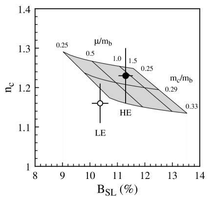
Figure 9: Combined theoretical predictions for the semileptonic branching ratio and charm counting as a function of the quark-mass ratio $m_{c}/m_{b}$ and the renormalization scale $\mu$. The data points show the average experimental values for $B_{\rm SL}$ and $n_{c}$ obtained in low-energy (LE) and high-energy (HE) measurements, as discussed in the text.

The combined theoretical predictions for the semileptonic branching ratio and charm counting are shown in Fig. 9. They are compared with the experimental results obtained from low- and high-energy measurements. It was argued that the combination of a low semileptonic branching ratio and a low value of $n_{c}$ would constitute a potential problem for the Standard Model [119]. However, with the new experimental and theoretical numbers, only for the low-energy measurements a small discrepancy remains between theory and experiment. Note that, using (84), our results for $n_{c}$ can be used to obtain a prediction for the branching ratio $B(\bar{B}\to X_{c\bar{c}s^{\prime}})$, which is accessible to a direct experimental determination. Our prediction of $(22\pm 6)\%$ for this branching ratio agrees well with the preliminary result reported by the CLEO Collaboration [114]: $B(\bar{B}\to X_{c\bar{c}s^{\prime}})=(23.9\pm 3.8)\%$.

5 Concluding Remarks

We have presented an introduction to the theory and phenomenology of heavy-flavour physics. The theoretical tools that allow us to perform quantitative calculations in this area are heavy-quark symmetry, the heavy-quark effective theory, and the $1/m_{Q}$ expansion. After presenting the underlying theoretical concepts, we have discussed their application to the description of exclusive and inclusive weak decays of $B$ mesons. Besides presenting the status of the latest developments, our hope was to convince the reader that heavy-flavour physics is a rich and diverse area of research, which is at present characterized by a fruitful interplay between theory and experiments. This has led to many significant discoveries and developments on both sides. Heavy-quark physics has the potential to determine many important parameters of the electroweak theory and to test the Standard Model at low energies. At the same time, it provides an ideal laboratory to study the nature of non-perturbative phenomena in QCD, still one of the least understood properties of the Standard Model.

Let us finish with a somewhat philosophical remark: In the last few years, there have been exciting developments in high-energy physics related to the discovery dualities, which relate apparently very different theories to each other. So are electric, weak-coupling phenomena in one theory dual to magnetic, strong-coupling phenomena in another theory. Some people argue quite convincingly that duality seems to be everywhere in nature, and consequently there are no really difficult questions in physics; very difficult problems become trivial when approached from a different, dual point of view. There are, however, “moderately difficult” problems in physics, which are “self-dual”. It is the author’s opinion that real-world (i.e. non-supersymmetric) QCD at hadronic energies belongs to this category. Having said this, we conclude that heavy-quark effective theory provides a powerful tool to tackle the “moderately difficult” problems of heavy-flavour physics.

References

References

- [1] C. Albajar et al. (UA1 Collaboration), Phys. Lett. B 186, 247 (1987).
- [2] H. Albrecht et al. (ARGUS Collaboration), Phys. Lett. B 192, 245 (1987).
- [3] H. Albrecht et al. (ARGUS Collaboration), Phys. Lett. B 234, 409 (1990); 255, 297 (1991).
-
[4]
R. Fulton et al. (CLEO Collaboration), Phys. Rev. Lett. 64,
16 (1990);
J. Bartelt et al. (CLEO Collaboration), Phys. Rev. Lett. 71, 4111 (1993). - [5] J.P. Alexander et al. (CLEO Collaboration), preprint CLNS-96-1419 (1996).
- [6] R. Ammar et al. (CLEO Collaboration), Phys. Rev. Lett. 71, 674 (1993).
- [7] M.S. Alam et al. (CLEO Collaboration), Phys. Rev. Lett. 74, 2885 (1995).
- [8] M. Neubert, Phys. Rep. 245, 259 (1994); Int. J. Mod. Phys. A 11, 4173 (1996).
- [9] M. Shifman, preprint TPI-MINN-95-31-T (1995) [hep-ph/9510377], to appear in: QCD and Beyond, Proceedings of the Theoretical Advanced Study Institute in Elementary Particle Physics (TASI 95), Boulder, Colorado, June 1995.
- [10] A. Falk, preprint JHU-TIPAC-96017 (1996) [hep-ph/9610363], to appear in: The Strong Interaction, from Hadrons to Partons, Proceedings of the 24th SLAC Summer Institute on Particle Physics, Stanford, California, August 1996.
- [11] H. Georgi, in: Perspectives in the Standard Model, Proceedings of the Theoretical Advanced Study Institute in Elementary Particle Physics (TASI-91), Boulder, Colorado, 1991, edited by R.K. Ellis, C.T. Hill, and J.D. Lykken (World Scientific, Singapore, 1992), p. 589.
- [12] N. Isgur and M.B. Wise, in: Heavy Flavours, edited by A.J. Buras and M. Lindner (World Scientific, Singapore, 1992), p. 234.
- [13] B. Grinstein, Ann. Rev. Nucl. Part. Sc. 42, 101 (1992).
- [14] T. Mannel, Chinese J. Phys. 31, 1 (1993).
- [15] A.G. Grozin, preprint Budker INP 92-97 (1992), unpublished.
- [16] K. Wilson, Phys. Rev. 179, 1499 (1969); D 3, 1818 (1971).
- [17] W. Zimmermann, Ann. Phys. 77, 536 and 570 (1973).
- [18] For a pedagogical introduction, see: H. Leutwyler, preprint [hep-ph/9609465], to appear in: Effectives Theories and Fundamental Interactions, Proceedings of the 34th International School of Subnuclear Physics, Erice, Italy, July 1996.
- [19] D.J. Gross and F. Wilczek, Phys. Rev. Lett. 30, 1343 (1973).
- [20] H.D. Politzer, Phys. Rev. Lett. 30, 1346 (1973).
- [21] The increase of the running coupling constant at low energies, as predicted by QCD, has been observed by analysing the hadronic-mass distribution in decays of the lepton, see: M. Girone and M. Neubert, Phys. Rev. Lett. 76, 3061 (1996).
- [22] E.V. Shuryak, Phys. Lett. B 93, 134 (1980); Nucl. Phys. B 198, 83 (1982).
-
[23]
J.E. Paschalis and G.J. Gounaris, Nucl. Phys. B 222, 473
(1983);
F.E. Close, G.J. Gounaris, and J.E. Paschalis, Phys. Lett. B 149, 209 (1984). - [24] S. Nussinov and W. Wetzel, Phys. Rev. D 36, 130 (1987).
- [25] M.B. Voloshin and M.A. Shifman, Yad. Fiz. 45, 463 (1987) [Sov. J. Nucl. Phys. 45, 292 (1987)].
- [26] M.B. Voloshin and M.A. Shifman, Yad. Fiz. 47, 801 (1988) [Sov. J. Nucl. Phys. 47, 511 (1988)].
- [27] N. Isgur and M.B. Wise, Phys. Lett. B 232, 113 (1989); 237, 527 (1990).
- [28] H. Georgi, Phys. Lett. B 240, 447 (1990).
- [29] N. Isgur and M.B. Wise, Phys. Rev. Lett. 66, 1130 (1991).
- [30] A.F. Falk, Nucl. Phys. B 378, 79 (1992).
- [31] A.F. Falk, M. Neubert, and M.E. Luke, Nucl. Phys. B 388, 363 (1992).
- [32] A.F. Falk and M. Neubert, Phys. Rev. D 47, 2965 and 2982 (1993).
- [33] I.J. Kroll, in: Proceedings of the 17th International Symposium on Lepton–Photon Interactions (LP95), Beijing, P.R. China, August 1995, edited by Z. Zhi-Peng and C. He-Sheng (World Scientific, Singapore, 1996), p. 204.
- [34] F. Ukegawa (for the CDF Collaboration), preprint FERMILAB-Conf-96/155-E (1996), to appear in: Proceedings of the XIth Topical Workshop on Collider Physics, Padova, Italy, May 1996.
- [35] P. Ball and V.M. Braun, Phys. Rev. D 49, 2472 (1994).
- [36] V. Eletsky and E. Shuryak, Phys. Lett. B 276, 191 (1992).
- [37] M. Neubert, Phys. Lett. B 322, 419 (1994); preprint CERN-TH/96-208 (1996) [hep-ph/9608211], to appear in Phys. Lett. B.
- [38] M. Neubert and V. Rieckert, Nucl. Phys. B 382, 97 (1992).
- [39] M. Neubert, Phys. Lett. B 264, 455 (1991).
- [40] M.E. Luke, Phys. Lett. B 252, 447 (1990).
- [41] M. Ademollo and R. Gatto, Phys. Rev. Lett. 13, 264 (1964).
- [42] M. Neubert, Nucl. Phys. B 416, 786 (1994).
- [43] P. Cho and B. Grinstein, Phys. Lett. B 285, 153 (1992).
- [44] H. Albrecht et al. (ARGUS Collaboration), Z. Phys. C 57, 533 (1993).
- [45] B. Barish et al. (CLEO Collaboration), Phys. Rev. D 51, 1041 (1995).
- [46] D. Buskulic et al. (ALEPH Collaboration), Phys. Lett. B 359, 236 (1995).
- [47] P. Abreu et al. (DELPHI Collaboration), preprint CERN-PPE/96-11 (1996).
- [48] S. Stone, in: Proceedings of the 8th Annual Meeting of the Division of Particles and Fields of the APS, Albuquerque, New Mexico, 1994, edited by S. Seidel (World Scientific, Singapore, 1995), p. 871.
-
[49]
C.G. Boyd, B. Grinstein and R.F. Lebed, Nucl. Phys. B 461,
493 (1996);
C.G. Boyd and R.F. Lebed, preprint UCSD/PTH 95-23 (1995) [hep-ph/9512363]. - [50] I. Caprini and M. Neubert, Phys. Lett. B 380, 376 (1996).
- [51] M. Neubert, Nucl. Phys. B 371, 149 (1992).
-
[52]
S.J. Brodsky, G.P. Lepage, and P.B. Mackenzie, Phys. Rev. D 28, 228 (1983);
G.P. Lepage and P.B. Mackenzie, Phys. Rev. D 48, 2250 (1993). - [53] M. Neubert, Phys. Lett. B 341, 367 (1995).
- [54] A.F. Falk and B. Grinstein, Phys. Lett. B 247, 406 (1990).
- [55] M. Neubert, Phys. Rev. D 46, 2212 (1992).
- [56] M. Neubert, Phys. Rev. D 51, 5924 (1995).
- [57] P. Ball, M. Beneke, and V.M. Braun, Phys. Rev. D 52, 3929 (1995).
- [58] A. Czarnecki, Phys. Rev. Lett. 76, 4124 (1996).
- [59] T. Mannel, Phys. Rev. D 50, 428 (1994).
- [60] M. Shifman, N.G. Uraltsev, and A. Vainshtein, Phys. Rev. D 51, 2217 (1995).
- [61] A. Kapustin, Z. Ligeti, M.B. Wise, and B. Grinstein, Phys. Lett. B 375, 327 (1996).
- [62] M. Neubert, Phys. Lett. B 338, 84 (1994).
- [63] For a pedagogical introduction, see: A. Manohar, preprint UCSD/PTH 96-04 (1996) [hep-ph/9606222], to appear in: Proceedings of the Schladming Winter School, Schladming, Austria, March 1996.
- [64] M.A. Shifman, A.I. Vainshtein, and V.I. Zakharov, Nucl. Phys. B 120, 316 (1977).
- [65] E. Witten, Nucl. Phys. B 122, 109 (1977).
- [66] J. Polchinski, Nucl. Phys. B 231, 269 (1984).
- [67] G. Altarelli and L. Maiani, Phys. Lett. B 52, 351 (1974).
- [68] M.K. Gaillard and B.W. Lee, Phys. Rev. Lett. 33, 108 (1974).
- [69] F.J. Gilman and M.B. Wise, Phys. Rev. D 27, 1128 (1983).
- [70] E. Eichten and F. Feinberg, Phys. Rev. D 23, 2724 (1981).
- [71] W.E. Caswell and G.P. Lepage, Phys. Lett. B 167, 437 (1986).
- [72] E. Eichten, in: Field Theory on the Lattice, edited by A. Billoire et al., Nucl. Phys. B (Proc. Suppl.) 4, 170 (1988).
- [73] G.P. Lepage and B.A. Thacker, in: Field Theory on the Lattice, edited by A. Billoire et al., Nucl. Phys. B (Proc. Suppl.) 4, 199 (1988).
- [74] H.D. Politzer and M.B. Wise, Phys. Lett. B 206, 681 (1988); 208, 504 (1988).
- [75] E. Eichten and B. Hill, Phys. Lett. B 234, 511 (1990).
- [76] B. Grinstein, Nucl. Phys. B 339, 253 (1990).
- [77] A.F. Falk, H. Georgi, B. Grinstein, and M.B. Wise, Nucl. Phys. B 343, 1 (1990).
- [78] E. Eichten and B. Hill, Phys. Lett. B 243, 427 (1990).
- [79] A.F. Falk, B. Grinstein, and M.E. Luke, Nucl. Phys. B 357, 185 (1991).
- [80] T. Mannel, W. Roberts, and Z. Ryzak, Nucl. Phys. B 368, 204 (1992).
- [81] J. Soto and R. Tzani, Phys. Lett. B 297, 358 (1992).
- [82] R. Tarrach, Nucl. Phys. B 183, 384 (1981).
- [83] M.A. Shifman, A.I. Vainshtein, and V.I. Zakharov, Nucl. Phys. B 147, 385 and 448 (1979).
- [84] G. ’t Hooft, in: The Whys of Subnuclear Physics, Proceedings of the 15th International School on Subnuclear Physics, Erice, Sicily, 1977, edited by A. Zichichi (Plenum Press, New York, 1979), p. 943.
- [85] B. Lautrup, Phys. Lett. B 69, 109 (1977).
- [86] G. Parisi, Phys. Lett. B 76, 65 (1978); Nucl. Phys. B 150, 163 (1979).
- [87] F. David, Nucl. Phys. B 234, 237 (1984); 263, 637 (1986).
- [88] A.H. Mueller, Nucl. Phys. B 250, 327 (1985).
- [89] V.I. Zakharov, Nucl. Phys. B 385, 452 (1992); M. Beneke and V.I. Zakharov, Phys. Rev. Lett. 69, 2472 (1992).
- [90] M. Beneke, Phys. Lett. B 307, 154 (1993); Nucl. Phys. B 405, 424 (1993).
- [91] D. Broadhurst, Z. Phys. C 58, 339 (1993).
- [92] A.H. Mueller, in: QCD – 20 Years Later, edited by P.M. Zerwas and H.A. Kastrup (World Scientific, Singapore, 1993), p. 162; Phys. Lett. B 308, 355 (1993).
- [93] M. Beneke and V.M. Braun, Nucl. Phys. B 426, 301 (1994).
- [94] I.I. Bigi, M.A. Shifman, N.G. Uraltsev, and A.I. Vainshtein, Phys. Rev. D 50, 2234 (1994).
- [95] M. Neubert and C.T. Sachrajda, Nucl. Phys. B 438, 235 (1995).
- [96] M. Beneke, V.M. Braun and V.I. Zakharov, Phys. Rev. Lett. 73, 3058 (1994).
- [97] M. Luke, A.V. Manohar and M.J. Savage, Phys. Rev. D 51, 4924 (1995).
- [98] J. Chay, H. Georgi, and B. Grinstein, Phys. Lett. B 247, 399 (1990).
-
[99]
I.I. Bigi, N.G. Uraltsev, and A.I. Vainshtein, Phys. Lett. B 293, 430 (1992) [E: 297, 477 (1993)];
I.I. Bigi, M.A. Shifman, N.G. Uraltsev, and A.I. Vainshtein, Phys. Rev. Lett. 71, 496 (1993);
I.I. Bigi et al., in: Proceedings of the Annual Meeting of the Division of Particles and Fields of the APS, Batavia, Illinois, 1992, edited by C. Albright et al. (World Scientific, Singapore, 1993), p. 610. - [100] B. Blok, L. Koyrakh, M.A. Shifman, and A.I. Vainshtein, Phys. Rev. D 49, 3356 (1994) [E: 50, 3572 (1994)].
- [101] A.V. Manohar and M.B. Wise, Phys. Rev. D 49, 1310 (1994).
-
[102]
M. Luke and M.J. Savage, Phys. Lett. B 321, 88 (1994);
A.F. Falk, M. Luke, and M.J. Savage, Phys. Rev. D 49, 3367 (1994). - [103] T. Mannel, Nucl. Phys. B 413, 396 (1994).
- [104] A.F. Falk, Z. Ligeti, M. Neubert, and Y. Nir, Phys. Lett. B 326, 145 (1994).
- [105] M. Neubert, Phys. Rev. D 49, 3392 and 4623 (1994).
- [106] I.I. Bigi, M.A. Shifman, N.G. Uraltsev, and A.I. Vainshtein, Int. J. Mod. Phys. A 9, 2467 (1994).
- [107] E.C. Poggio, H.R. Quinn, and S. Weinberg, Phys. Rev. D 13, 1958 (1976).
-
[108]
M. Shifman, Minneapolis preprint TPI-MINN-95/15-T (1995)
[hep-ph/9505289], to appear in: Proceedings of the Joint Meeting of
the International Symposium on Particles, Strings and Cosmology and
the 19th Johns Hopkins Workshop on Current Problems in Particle
Theory, Baltimore, Maryland, March 1995;
B. Chibisov, R.D. Dikeman, M. Shifman, and N. Uraltsev, preprint TPI-MINN-96-05-T (1996) [hep-ph/9605465]. - [109] F.G. Gilman and M.B. Wise, Phys. Rev. D 20, 2392 (1979).
- [110] G. Altarelli, G. Curci, G. Martinelli, and S. Petrarca, Phys. Lett. B 99, 141 (1981); Nucl. Phys. B 187, 461 (1981).
- [111] A.J. Buras and P.H. Weisz, Nucl. Phys. B 333, 66 (1990).
- [112] Y. Nir, Phys. Lett. B 221, 184 (1989).
- [113] M. Neubert, in: Proceedings of the 17th International Symposium on Lepton–Photon Interactions (LP95), Beijing, P.R. China, August 1995, edited by Z. Zhi-Peng and C. He-Sheng (World Scientific, Singapore, 1996), p. 298; Int. J. Mod. Phys. A 11, 4173 (1996).
- [114] K. Honscheid, these Proceedings.
- [115] T. Skwarnicki, in: Proceedings of the 17th International Symposium on Lepton–Photon Interactions (LP95), Beijing, P.R. China, August 1995, edited by Z. Zhi-Peng and C. He-Sheng (World Scientific, Singapore, 1996), p. 238.
- [116] P. Perret, Clermont-Ferrand preprint PCCF-RI 9507 (1995), to appear in: Proceedings of the International Europhysics Conference on High Energy Physics, Brussels, Belgium, July–August 1995.
- [117] G. Altarelli and S. Petrarca, Phys. Lett. B 261, 303 (1991).
- [118] H. Simma, G. Eilam and D. Wyler, Nucl. Phys. B 352, 367 (1991).
- [119] G. Buchalla, I. Dunietz and H. Yamamoto, Phys. Lett. B 364, 188 (1995).
- [120] T. Browder, preprint UH 511-836-95 (1995), to appear in: Proceedings of the International Europhysics Conference on High Energy Physics, Brussels, Belgium, July–August 1995 [hep-ex/9602009].
-
[121]
G. Calderini, presented at the 31th Rencontres de Moriond: QCD and
High Energy Hadronic Interactions, Les Arcs, France, March 1996;
D. Buskulic et al. (ALEPH Collaboration), preprint CERN-PPE/96-117 (1996). - [122] I. Bigi, B. Blok, M.A. Shifman, and A. Vainshtein, Phys. Lett. B 323, 408 (1994).
-
[123]
E. Bagan, P. Ball, V.M. Braun, and P. Gosdzinsky, Nucl. Phys. B
432, 3 (1994); Phys. Lett. B 342, 362 (1995) [E: 374, 363 (1996)];
E. Bagan, P. Ball, B. Fiol, and P. Gosdzinsky, Phys. Lett. B 351, 546 (1995). - [124] M. Neubert and C.T. Sachrajda, preprint CERN-TH/96-19 (1996) [hep-ph/9603202], to appear in Nucl. Phys. B.
- [125] M. Luke, M.J. Savage, and M.B. Wise, Phys. Lett. B 343, 329 (1995); 345, 301 (1995).